consistent estimation of the fixed effects ordered logit model - iza
TRANSCRIPT

DI
SC
US
SI
ON
P
AP
ER
S
ER
IE
S
Forschungsinstitut zur Zukunft der ArbeitInstitute for the Study of Labor
Consistent Estimation of the Fixed Effects Ordered Logit Model
IZA DP No. 5443
January 2011
Gregori BaetschmannKevin E. StaubRainer Winkelmann
Consistent Estimation of the
Fixed Effects Ordered Logit Model
Gregori Baetschmann University of Zurich
Kevin E. Staub
University of Zurich
Rainer Winkelmann University of Zurich,
CESifo and IZA
Discussion Paper No. 5443 January 2011
IZA
P.O. Box 7240 53072 Bonn
Germany
Phone: +49-228-3894-0 Fax: +49-228-3894-180
E-mail: [email protected]
Any opinions expressed here are those of the author(s) and not those of IZA. Research published in this series may include views on policy, but the institute itself takes no institutional policy positions. The Institute for the Study of Labor (IZA) in Bonn is a local and virtual international research center and a place of communication between science, politics and business. IZA is an independent nonprofit organization supported by Deutsche Post Foundation. The center is associated with the University of Bonn and offers a stimulating research environment through its international network, workshops and conferences, data service, project support, research visits and doctoral program. IZA engages in (i) original and internationally competitive research in all fields of labor economics, (ii) development of policy concepts, and (iii) dissemination of research results and concepts to the interested public. IZA Discussion Papers often represent preliminary work and are circulated to encourage discussion. Citation of such a paper should account for its provisional character. A revised version may be available directly from the author.

IZA Discussion Paper No. 5443 January 2011
ABSTRACT
Consistent Estimation of the Fixed Effects Ordered Logit Model* The paper re-examines existing estimators for the panel data fixed effects ordered logit model, proposes a new one, and studies the sampling properties of these estimators in a series of Monte Carlo simulations. There are two main findings. First, we show that some of the estimators used in the literature are inconsistent, and provide reasons for the inconsistency. Second, the new estimator is never outperformed by the others, seems to be substantially more immune to small sample bias than other consistent estimators, and is easy to implement. The empirical relevance is illustrated in an application to the effect of unemployment on life satisfaction. JEL Classification: C23, C25, J28, J64 Keywords: ordered response, panel data, correlated heterogeneity, incidental parameters Corresponding author: Rainer Winkelmann University of Zurich Department of Economics Zürichbergstr. 14 CH-8032 Zürich Switzerland E-mail: [email protected]
* We thank Paul Frijters, Arie Kapteyn and participants of 2011 Engelberg Workshop in Labor Economics for very valuable comments on an earlier draft.

1 Introduction
Economists’ use of panel data has been increasing steadily over the past years. As a key
advantage, such data potentially allow to solve the endogeneity problem arising from cor-
related time-invariant unobserved individual-specific effects. However, while implementing
corresponding estimators is straightforward if the model is linear, no generally valid method
exists for non-linear models.
One important application of non-linear models arises in the context of responses that
are coded on a discrete and ordinal scale. Such scales are prominent in many household
surveys, where they provide information on subjective assessments, judgments, or expec-
tations. Examples are an individuals’ satisfaction (with one’s job, life in general, etc.) or
expectations about the future (of the economy, of one’s income, etc.). There are good
reasons for using such subjective evaluations in empirical research, for example because
they substitute for objective information that is not collected, or because the subjective
responses are of their own interest. For instance, subjective health status might be more
closely tied to certain behavioral responses than actual health.
The most popular regression-type models for such dependent variables are the ordered
probit model and, in particular, the ordered logit model. With cross-section data, these
parametric models are very easy to use and to estimate by maximum likelihood. However,
extensions to a panel data context are complex and far from obvious. Unlike in the linear
model, no simple transformation (such as first-differencing or within-transformation) is
available that would purge the ordered response models from the individual-specific fixed
effects.
While the situation is hopeless for the ordered probit model, it is more favorable for the
ordered logit model, where it has been recognized early on that the estimation problem can
be simplified to that of a binary logit model for which a fixed effects estimator exists, by
collapsing the J categorical responses into two classes (e.g. Winkelmann and Winkelmann,
1998). The binary logit fixed effects estimator, due to Chamberlain (1980), uses the fact
1

that conditioning the individual likelihood contribution on the sum of the outcome over
time provides an expression which is independent of the fixed effects. The effect of the
time-varying regressors can then be estimated by conditional maximum likelihood (CML).
Other popular estimators for the fixed effects ordered logit model proposed in the lit-
erature are also built around the same idea of reducing the ordered model to a binary one,
but aim at improving over a simple dichotomization by exploiting additional information
available in the data. One approach is to estimate fixed effects logits with every possible
dichotomizing cutoff point, and then combine the resulting estimates by minimum distance
estimation (Das and van Soest, 1999).
A second approach is to dichotomize every individual separately, at some sort of ‘op-
timal’ or ‘efficient’ cutoff point (Ferrer-i-Carbonell and Frijters, 2004). The most popular
variant dichotomizes the dependent variable at the individual mean, which ensures that
every individual displaying some time variation in the outcome is included in the estima-
tion. Such fixed effects ordered logit models have been used frequently in the literature.
Recent applications to health economics include Jones and Schurer (2009), and Frijters,
Haisken-DeNew and Shields (2004 a, b); additions to the satisfaction literature comprise
Kassenboehmer and Haisken-DeNew (2009), Booth and van Ours (2008), D’Addio, Eriks-
son and Frijters (2007), and Frijters, Haisken-DeNew and Shields (2004).
In this article we propose a new consistent estimator for the ordered logit model with
fixed effects. We then compare the existing and the new estimators in Monte Carlo sim-
ulations. There are two important findings which have implications for future applied
research based on panel ordered logit models. First, we observe that individual-specific
dichotomized estimators are biased in finite samples. Worse, the bias does not vanish as
simulations with increased sample size are considered. We provide reasons for this obser-
vation, and show that, in general, these estimators are inconsistent. The problem is that
by choosing the cutoff point based on the outcome, they produce a form of endogeneity.
Second, we provide evidence on the good finite sample performance of Das and van Soest’s
2

(1999) estimator and our new estimator. In contrast to Das and van Soest’s (1991), the
new estimator remains unbiased even in very small samples. Moreover, it can be easily
implemented using existing software for CML logit estimation.
The paper proceeds as follows. Section 2 presents the different estimators for the fixed
effects ordered logit models. Then, we explain our Monte Carlo simulation setup and
discuss its results (Section 3), followed by an application of the estimators to data from the
German Socioeconomic Panel which studies the effect of unemployment on life satisfaction
(Section 4). Section 5 concludes.
2 Estimators for the FE ordered logit model
2.1 The FE ordered logit model
The fixed effects ordered logit model relates the latent variable y∗it for individual i at time
t to a linear index of observable characteristics xit and unobservable characteristics αi and
εit:
y∗it = x′itβ + αi + εit, i = 1, . . . , N t = 1, . . . , T (1)
The time-invariant part of the unobservables, αi, can be statistically dependent of xit. In
this case, one can either make an assumption regarding the joint distribution of αi and xit,
or else treat αi as a fixed effect. This paper considers estimation under the fixed effects
approach.
The latent variable is tied to the (observed) ordered variable yit by the observation rule:
yit = k if τk < y∗it ≤ τk+1, k = 1, . . . , K
where thresholds τ are assumed to be strictly increasing (τk < τk+1 ∀k) and τ1 = −∞,
τK+1 = ∞. It is possible to formulate the model more generally with individual-specific
thresholds (Ferrer-i-Carbonell and Frijters, 2004):
yit = k if τik < y∗it ≤ τik+1, k = 1, . . . , K (2)
3
The distributional assumption completing the specification of the fixed effects ordered
logit model is that conditionally on xit and αi, εit are IID standard logistically. I.e., if F (·)
denotes the cdf of εit
F (εit|xit, αi) = F (εit) =1
1 + exp(−εit)≡ Λ(εit) (3)
Hence, the probability of observing outcome k for individual i at time t using (1), (2),
(3) is
Pr(yit = k|xit, αi) = Λ(τik+1 − x′itβ − αi)− Λ(τik − x′itβ − αi) (4)
which depends not only on β and xit, but also on αi and τik,τik+1.
There are two problems with Maximum Likelihood (ML) estimation based on expression
(4). The first is a problem of identification: τik cannot be distinguished from αi; only
τik−αi ≡ αik is identified and can thus, in principle, be estimated consistently for T →∞.
The second problem arises, since in most applications, T must be treated as fixed and
relatively small. But under fixed-T asymptotics even αik cannot be estimated consistently,
due to the incidental parameter problem (see, for instance, Lancaster, 2000). This does
have consequences for estimation of β – the bias in αik contaminates β. In short panels,
the resulting bias in β can be substantial (Greene, 2004).
We next consider different approaches to estimate β consistently. They all use the
same idea of collapsing yit into a binary variable and then applying the sufficient statistic
suggested by Chamberlain (1980) to construct a CML estimator.
2.2 Chamberlain’s CML estimator for the dichotomized ordered
logit model
Let dkit denote the binary dependent variable that results from dichotomizing the ordered
variable at the cutoff point k: dkit = 1(yit ≥ k). By construction, P (dkit = 0) = P (yit < k) =
Λ(τik+1− x′itβ−αi), and P (dkit = 1) = P (yit ≥ k) = 1−Λ(τik+1− x′itβ−αi). Now consider
4

the joint probability of observing di = (dki1, . . . , dkiT ) = (ji1, . . . , jiT ) with jit ∈ 0, 1. The
sum of all the individual outcomes over time is a sufficient statistic for αi as
Pki (β) ≡ Pr
(dki = ji
∣∣∣∣∣T∑t=1
dkit = ai
)=
exp(j′ixiβ)∑j∈Bi
exp(j′xiβ)(5)
does not depend on αi and the thresholds. In (5), ji = (ji1, . . . , jiT ), xi is the (T×L)-matrix
with tth row equal to xit, L is the number of regressors and ai =∑T
t=1 jit . The sum in the
denominator goes over all vectors j which are elements of the set Bi
Bi =
j ∈ 0, 1T
∣∣∣∣∣T∑t=1
jt = ai
,
i.e., over all possible vectors of length T which have as many elements equal to 1 as the
actual outcome of individual i (ai). The number of j-vectors in Bi, and therefore of terms
in the sum in the denominator of (5), is(Tai
)= T !
ai!(T−ai)!.
Chamberlain (1980) shows that maximizing the conditional likelihood
logLk(b) =N∑i=1
logPki (b) (6)
gives a consistent estimate for β (subject to mild regularity conditions on the distribution
of αi, cf. Andersen, 1970). I.e. the score —the gradient of the log-likelihood with respect
to β— converges to zero when evaluated at the true β:
plim1
N
∑i
ski (β) = 0, (7)
where
ski (b) =∂ lnPki (b)
∂b= x′i
(dki −
∑j∈Bi
jexp(j′xib)∑l∈Bi
exp(l′xib)
)(8)
The reason why (7) holds is that for every i, conditional on xi, the expectation of the term
in parentheses in (8) is zero as it defines a conditional expectation residual.
Note that conditioning on ai causes all time-invariant elements in (4) to cancel. I.e.,
not only αi and τik+1 are not estimated, but also elements of the β vector corresponding
to observables that do not change over time. Also, individuals with constant dkit do not
5

contribute to the conditional likelihood function, as P (dki = 1|∑T
t=1 dkit = T ) = P (dki =
0|∑T
t=1 dkit = 0) = 1.
The Hessian is
Hki (b) =
∂2 lnPki (b)
(∂b)(∂b)′= −
∑j∈Bi
exp(j′xib)∑l∈Bi
exp(l′xib)×
(x′ij −
∑m∈Bi
exp(m′xib)∑l∈Bi
exp(l′xib)m′xi
)(x′ij −
∑m∈Bi
exp(m′xib)∑l∈Bi
exp(l′xib)m′xi
)′(9)
2.3 Combining all possible dichotomizations: Das and van Soest’s
(1999) two-step estimation, and a new approach
The estimator of β based on (6), say βk, does not use all the variation in the ordered
dependent variable yit, as individuals for which either yit < k or yit ≥ k for every t do
not contribute to the log-likelihood. Since every βk for k = 2, . . . , K provides a consistent
estimator of β, and every individual with some variation in yit will contribute to at least one
log-likelihood Lk(b), one can perform CML estimation on all possible K−1 dichotimizations
and then, in a second step, combine the resulting estimates. The efficient combination will
weight the βk by the inverse of their variance (Das and van Soest, 1999):
βDvS = arg minb
(β2′ − b′, . . . , βK′ − b′)Ω−1(β2′ − b′, . . . , βK′ − b′)′ (10)
The variance Ω has entries ωgh, g = 2, . . . , K, h = 2, . . . , K, such that
ωgh =[E(∂ logPg
∂b
)(∂ logPg
∂b
)′]−1 [E(∂ logPg
∂b
)(∂ logPh
∂b
)′][E(∂ logPhi∂b
)(∂ logPh
∂b
)′]−1
evaluated at b = β. In practice, the unknown variance Ω is replaced by an estimate Ω
which is evaluated at βk, k = 2, . . . , K. The solution to (10) is
βDvS =(H ′Ω−1H
)−1H ′Ω−1(β2′
, . . . , βK′)′
6

where H is the matrix of K-1 stacked identity matrices of dimension L (the size of each
βk). An estimate of the variance of the estimator can be obtained as
Var(βDvS) =(H ′Ω−1H
)−1
Because βDvS is a linear combination of consistent estimators, it is itself consistent. Ferrer-
i-Carbonell and Frijters (2004) discuss some small sample issues which might affect the
performance of βDvS. For instance, one concern is that Ω might be estimated very impre-
cisely when for some g and h there are only few observations with nonzero contributions to
ωgh. This is the case when there is only a small overlap between the samples contributing
to the CML logit estimator dichotomized at g and the one dichotomized at h.
Thus, we propose an alternative to this two-step combination of all possible dichotomiza-
tions which avoids such problems by estimating all dichotomizations jointly subject to the
restriction βk = β ∀k = 2, . . . , K. Hence, the sample (quasi-) log-likelihood of this re-
stricted CML estimator is
logL(b) =K∑k=2
logLk(b) (11)
The score of this estimator is the sum of the scores of the CML logit estimators. Since these
estimators are consistent, their scores converge to zero in probability. It follows that the
probability limit of the score of the restricted CML estimator is zero as well, establishing
its consistency:
plimK∑k=2
1
N(K − 1)
N∑i=1
ski (β) = plim1
N
∑i
s2i (β) + . . .+ plim
1
N
∑i
sKi (β) = 0, (12)
Since some individuals contribute to several terms in the log-likelihood this creates depen-
dence between these terms, invalidating the usual estimate of the estimator variance based
on the information matrix equality. Instead, a sandwich variance estimator (White, 1982)
should be used. We propose using the cluster-robust variance estimator which allows for
arbitrary correlation within the various contributions of any individual:
Var(β) =
(N∑i=1
hi
)−1( N∑i=1
sis′i
)−1( N∑i=1
hi
)−1
7

where si are the stacked CML scores of individual i evaluated at β, si = (s2′i , . . . , s
K′i )′, and
hi is the matrix of derivatives of si with respect to β evaluated at β.
We will refer to this estimator as the BUC estimator. The acronym stands for “Blow-
Up and Cluster” which describes the way of implementing this estimator using the CML
estimator: Replace every observation in the sample by K − 1 copies of itself (“blow-up”
the sample size), and dichotomize every K − 1 copy of the individual at a different cutoff
point. Estimate CML logit using the entire sample; these are the BUC estimates. Cluster
standard errors at the individual level. This implementation requires but a few lines of code
in standard econometric software (cf. Appendix A, which contains code for implementation
in Stata).
2.4 Endogenous dichotomization: Ferrer-i-Carbonell and Frijters
(2004) and related approaches
The previous approaches used all possible dichotomizations. Ferrer-i-Carbonell and Fri-
jters (2004) proposed an estimator which chooses dichotomizations separately for every
individual. The (quasi-) log-likelihood for their estimator can be written as
logLFF (b) =N∑i=1
K∑k=2
wki logPki (b), wki ∈ 0, 1,K∑k=2
wki = 1 (13)
This objective function is maximized with respect to b after choosing the cutoff point at
which to dichotomize each yi, i.e. after deciding which one of the individual’s weight vectors
wki is equal to 1.
Ferrer-i-Carbonell and Frijters’ (2004) approach here is to calculate for every individual
all Hessian matrices under different cutoff points and choosing the smallest:
wki = 1 if k = arg minκ
∂2 logPκi (b)
(∂b)(∂b)′
∣∣∣b=β
In practice, the Hessian is evaluated at β, where β is a preliminary consistent estimator.
Since for every possible dichotomization the choice falls on the cutoff point leading to the
8
smallest Hessian, this rule should yield the estimator of (13) with minimal variance. Other,
simpler rules for choosing wki for (13) have been used, trading efficiency for computational
ease. In fact, the standard way in which this estimator is implemented in the applied
literature is by choosing the dichotomizing cutoff point as the mean of the dependent
variable:
wki = 1 if k = ceil
(T−1
∑t
yit
)
where ceil(z) stands for rounding z up to the nearest integer. This ensures that every
individual with time-variation in yi will be part of the estimating sample. Studies using
both rules report little difference in estimates and standard errors, which has led to the
view that this way of choosing wki is an approximation to Ferrer-i-Carbonell and Frijters’
(2004) . An alternative is using the median instead of the mean as a rule to define the
individual dichotomization.
Thus, all these procedures choose the dichotomizing cutoff point endogenously, since
it depends on yi. This is obviously problematic and we show in Appendix B that these
estimators are, in general, inconsistent. Here we provide some intuition for this result using
the mean-cutoff estimator as an example; similar arguments hold for the other estimators.
The problem is not, as one might suspect, that the cutoffs vary between individuals
per se. For instance, if the variation of the cutoffs between individuals was random, the
resulting estimator would be consistent: the score would be a sum of scores of CML logit
estimators, much like the BUC estimator (but with K − 1 times less observations as each
individual would contribute only to exactly one CML logit estimator). I.e., in terms of
(8), for every random individual-specific cutoff, the resulting vectors di converge to their
respective conditional expectation, yielding an expected score of zero at the limit.
The real problem lies in the endogeneity of the cutoff. For the mean estimator, dMnit = 1
if and only if yit ≥ T−1∑
t yit. Thus, yit itself is part of the cutoff and the probability
9

Pr(dMnit = 1) can be written as
Pr(dMnit = 1) = Pr
(yit ≥
1
T
∑t
yit
)= Pr
(yit ≥
1
T − 1
∑s 6=t
yis
)The expression after the first equality makes clear that for any t, yit is on both sides of
the inequality sign. Solving for yit shows that the probability Pr(dit = 1) is equal to
the probability that the outcome in t is greater than the average outcome in the remaining
periods. In general, this is a different dichotomizing cutoff point within the same individual
for every period. Thus, although the researcher is setting an individual-specific cutoff, say k,
the endogenous way in which this cutoff is chosen implies that it is equivalent to choosing
different cutoff points for the same individual. With endogenous cutoffs the conditional
distribution of di can be shown to differ from the CML terms, and the score of these
estimators will, in general, not converge to zero.
3 Monte Carlo simulations
We compare the performance of the estimators discussed in the previous section in finite
samples using Monte Carlo simulations. To the best of our knowledge, this is the first
investigation of these estimators in a Monte Carlo study. The aim is to assess the small
sample biases and efficiency across different data generating processes.
3.1 Experimental design
The setup of the Monte Carlo experiment is as follows. The data generating process (DGP)
for the latent variable is
y∗it = βxxi,t + βddi,t + αi + εit,
and we set βx = 1, βd = 1. The regressor x is continuous, while d is binary. We follow
Greene (2004) in specifying the fixed effects as
αi =√T xi +
√T ui, xi = T−1
∑t
xit, ui = T−1∑t
uit, uit ∼ N(0, 1)
10
For the simulations, we use fixed (not individual-specific) thresholds:
yit = k if τk < y∗it ≤ τk+1, k = 1, . . . , K
Finally, εit is sampled from a logistic distribution as in (3).
The baseline DGP is a balanced panel of N=500 individuals observed for T=4 periods.
The continuous regressor x is distributed as standard normal, the binary regressor’s prob-
ability of a 1 is 50%. The latent variable is discretized into K=5 categories, choosing the
thresholds to yield the marginal distribution depicted in the upper left graph in Fig. 1. We
call this distribution of y “skewed”.
The baseline DGP is modified in a number of dimensions, which can be broadly classified
into two experiments. First, different kinds of asymptotics are considered by increasing N,
T and K. Second, the influence of the data distribution is explored by sampling from
different distributions from the regressors, and by shifting the thresholds to yield different
marginal distributions for yit. In the following section, we comment on selected results
from these experiments. A supplementary appendix containing full simulation output from
a comprehensive exploratory study is available from the authors on request.
3.2 Results
Table 1 contains results for the baseline scenario. Columns contain mean and standard
deviation of estimated coefficients (labeled M and SD), as well as the mean of standard
errors (labeled SE) corresponding to x (first three columns) and d (last three columns).
Every row gives these results for a different estimator. All entries have been rounded to
two decimal places.
The first row, named DvS, contains results for the two-step estimator of Das and van
Soest (1999). With means of 0.99 for βx and 1.00 for βd DvS is virtually unbiased. The
BUC estimator, whose results are displayed in the second row, produces unbiased results,
too. There is almost no perceivable difference in efficiency between the two estimators.
11

Estimation of the coefficient corresponding to the binary variable is less precise than that
of the continuous regressor — its standard deviation is around 60% higher.
The next three rows contain results for Ferrer-i-Carbonell and Frijters’ (2004) estimator
(named FF), as well as for the variants dichotomizing at the individual mean (labeled
Mean) and at the individual median (labeled Median). These three estimators display
standard deviations of the same size as BUC’s and DvS’. However, their means shows a
clear downward bias. E.g., for βx, it ranges from 7% for FF to 4% for Mean. With a
standard deviation of 0.07 and 1,000 replications, the margin of error at 99% confidence
for these biases is less than 0.6%-points.
The last four rows contain results for CML logit estimators dichotomized at the cate-
gories 2 to 5 (named ‘y ≥ 2’ to ‘y ≥ 5’). As DvS and BUC, these estimators show little
finite sample bias. The standard deviations are at best about 30% larger than BUC’s —
this corresponds to cases where the dichotomized dependent variable has a distribution
which is as balanced as possible. For ‘y ≥ 2’ and ‘y ≥ 3’ the percentage of zeros is 40%
and 70%. For ‘y ≥ 5’ this percentage is 95%, and the standard deviation of the estimator
is more than double that of BUC.
Comparing columns containing the standard deviations of the estimators (SD) with
columns containing average standard errors (SE) shows that standard errors are estimated
satisfactorily in all cases.
Taken together, the results of Table 1 contain two important findings. First, there is no
evidence that finite sample issues affect the DvS estimator. All estimators exploiting more
information in the data than CML logit estimators with fixed cutoffs are, indeed, more
efficient than them. However, they all display about the same standard deviation. Second,
estimators based on endogenous dichotomizing cutoff points are all biased in this setup.
Next, we want to check whether these results can be generalized to other settings. We
start by conducting asymptotic exercises to explore under which conditions the biases of
FF, Mean and Median can be expected to vanish. The results are reported in Table 2.
12

The first panel of Table 2 (‘Baseline scenario’), consisting of the first four columns, copies
the results from Table 1 for easier comparability. Columns with averages of standard errors
(SE) were dropped to avoid clutter; we found that results for SE were similar to Table
1’s for all DGPs considered in this paper. In the second panel (‘N=1,000’, the next four
columns) the effect of increasing sample size with fixed T is considered. As expected by
the ratio√
500/√
1, 000 the standard deviation falls by 30% for all estimators. As before,
DvS and BUC are unbiased. However, FF, Mean and Median estimators remain biased.
Indeed, their bias is essentially the same with 1,000 individuals as with 500. This suggests
that these are not small sample biases, but that they can be attributed entirely to these
estimators’ inconsistency.
A different asymptotic experiment holds N fixed and increases the number of time
periods. Based on the discussion of the inconsistency of estimators with endogenous di-
chotomization, we would expect this to have an attenuating impact on their biases: As
T increases, the contribution of any yit to the endogenous cutoff (a function of all yit
of an individual) decreases. If its contribution was zero, the cutoff would be exogenous.
For instance, this is particularly transparent for the mean estimator. In the probability
Pr(dMnit = 1) = Pr
(yit ≥ 1
T−1
∑s 6=t yis
), the threshold consisting of the average yis, s 6= t,
becomes less variable for different t as T increases.
The results for this experiment are reported in the next panel, labeled ‘T=8’, where
the number of time periods in the simulations were duplicated from T=4 to T=8. The
decrease in the standard deviations relative to the Baseline scenario is roughly of the same
magnitude as in the experiment with N=1,000. Clearly, the biases of FF, Mean and Median
are reduced, consistent with our expectation.
A last kind of informal asymptotic experiment which can be conceived is increasing the
number of categories. In the limit, the observed variable would be equal to the continuous
latent variable. We increase the number of categories from K=5 to K=10, setting the
marginal distribution to the one displayed in the lower right panel of Fig. 1. While this
13
distribution is skewed, too, it is of course not exactly the same as in the baseline case.
The results are displayed in the fourth panel in Table 2, labeled ‘K=10’. There are now
5 additional CML logit estimators (y ≥ 6 to y ≥ 10), but for the sake of brevity we omit
results for these. While Dvs and BUC are almost invariant to the increase in the number
of ordered categories, the three estimators based on endogenous dichotomization worsen in
terms of bias. This, too, is to be expected. With increasing K and fixed T, the sensitivity of
endogenous cutoffs to a particular yit will increase in general. For the mean estimator, for
instance, the variance in the mean yis, s 6= t increases with K. It is interesting to note that
the median estimator suffers more severely from increasing K, which is in line with the fact
that the variance of the median yit is larger than that of the mean yit in our distributions
of yit.
A noteworthy constant in the discussion of results so far has been the equally good
performance of DvS and BUC. This is remarkable as previous literature raised the concern
that the DvS estimator could show difficulties when confronted with small samples for the
different CML logit estimates. In the setup with K=10 and N=500 the last two CML
logit estimators (k=9 and k=10) used on average about 137 and 78 individuals. DvS is
only slightly (but statistically significantly) biased downwards. The last panel in Table 2
shows the results from a smaller sample of N=100 while maintaining K=10. This produces
a difficult DGP for DvS, as only about 28 and 29 individuals are used in the CML logit
estimations of k=9 and k=10. This resembles the situation in life satisfaction studies,
where responses in lower categories are extremely infrequent (Ferrer-i-Carbonell and Fri-
jters, 2004). Here we do find biases of -6% and -7% for DvS (margin of error at 99%: 1%-
and 2%-points, respectively). The BUC estimator in contrast remains as unbiased as in
previous DGPs. FF, Median and Mean estimators also show little change and are as biased
as with N=500.
The influence of the distribution of the data on the performance of the estimators is
addressed in the DGPs whose results are shown in Table 3. Again, the first panel repeats
14

the results for the baseline case from Table 1. The next two panels —with headings ‘bell-
shaped y’ and ‘uniform y’ — show results for different marginal distributions of yit. I.e., all
parameters from the baseline DGP are kept unchanged, except for thresholds τ which have
been shifted to yield these distributions (cf. Fig. 1). These changes in yit seem to have close
to no impact on the performance of the estimators. Only CML logit estimators are affected
in their precision. It is no surprise that, for given distribution of x, d, the more balanced
the distribution of the dichotomized variable, the higher the precision of the resulting CML
logit estimator. The last panel in Table 3 resets the thresholds to their baseline values and
changes the distribution of the explanatory variables. The continuous x is now drawn from
a log-normal distribution, standardized to have mean zero and unit variance; the binary
d’s new distribution is highly unbalanced with only 10% of observations having d = 1 on
average. As before, the picture remains by and large the same: All estimators show higher
standard deviations in this DGP, but the ranking is unchanged.
4 Application: Why are the unemployed so unhappy?
The preceding section documented the performance of different estimators for the fixed
effects ordered logit model in simulations. In this section, the estimators are used to reesti-
mate the effect of unemployment on life satisfaction using the dataset of Winkelmann and
Winkelmann (1998). The data consists of a large sample from the German Socioeconomic
Panel, totaling at 20,944 observations; the model includes 9 explanatory variables. With
these values, the application provides a typical setting to which the estimators have been
put to use and are likely to be applied in the future.
4.1 Data and specification
The sample consists of the first six consecutive waves of the German Socioeconomic Panel
going from 1984 to 1989. It includes all observations of persons aged 20-64 years with
15
participation in at least two waves and non-missing responses for all variables of the model.
These are 20,944 person-year observations corresponding to 4,261 individuals. Of these,
1,873 observations corresponding to 303 persons are discarded because they do not dis-
play any variation over time in their outcome variable, leaving the dataset with 19,079
observations corresponding to 3,958 individuals.
The outcome variable is satisfaction with life which is measured as the answer to the
question “How satisfied are you at present with your life as a whole?”. The answer can
be indicated in 11 ordered categories ranging from 0, “completely dissatisfied”, to 10,
“completely satisfied”.
The key explanatory variables are a set of three dummy variables which indicate cur-
rent labor market status: Unemployed, Employed and Out of labor force. These dummies
exhaust the possible labor market status and are mutually exclusive, so Employed is used
as the omitted reference category in the model.
Additional information about psychological costs of unemployment might be revealed
through the length of the unemployment spell. Thus, the model contains the variables
Duration of unemployment and Squared duration of unemployment.
Demographic control variables include marital status (Married), health status (Good
health), age (Age and Squared age) and household income (in logarithms, Log. household
income). We refer to the original source for comprehensive descriptions of data and speci-
fication.
4.2 Results
Estimation results are presented in Table 4. Every column depicts results of the same
model for a different estimator. The first replicates the original results in Winkelmann and
Winkelmann (1998, Table 4, column 2, p.11) who used a CML logit estimator dichotomized
at the cutoff 8. This cutoff results in a distribution of the binary dependent variable which
is about balanced with around 50% of the responses being equal or greater than 8. In
16

total 2,573 individuals cross this cutoff resulting in an estimating sample size of 12,980
observations.
To briefly summarize the results, the effect of unemployment is found to be both large
and statistically significant; there is no effect of unemployment duration on life satisfac-
tion, so there seems to be no mental adaptation process of unemployed persons to their
status. Coefficients of socio-demographic variables display expected signs and magnitudes
(cf. Clark and Oswald, 1994).
Moving to the right of the table, the next two columns correspond to results obtained
using the DvS and BUC estimators, and the final three columns show results for FF, Mean
and Median estimates. The most striking feature of the results as a whole is that the first
three columns —which are based on consistent estimators— are remarkably similar, while
they differ from the three last columns containing estimates from inconsistent estimators.
The marginal effect of unemployment on latent life satisfaction is estimated to be around -1
when using CML logit, DvS or BUC; but it ranges only from -0.84 to -0.66 when using FF,
Mean or Median estimators. Similarly, effects for marital status and age are estimated to be
larger using either of the consistent estimators. Although estimation is not precise enough
to reject equality of coefficients, these results clearly echo patterns from the Monte Carlo
simulations. There is only one clear difference between consistent estimators. It relates to
the coefficient of Out of labor force, which is -0.24 and insignificant for CML logit while
being around -0.45 and significant for DvS and BUC. A potential explanation for this is
that most of the changes in Out of labor force occur at levels of satisfaction lower than the
cutoff used by the CML logit estimator, so that this information is lost to the CML logit
estimation. DvS and BUC, on the other hand, use all 3,958 persons displaying some time
variation in life satisfaction (for BUC the number of persons corresponds to the number of
clusters; the number of individuals is the cross-sectional dimension of the “blown-up” or
inflated sample).
All estimators display similarly sized standard errors. CML logit estimates are the
17

largest, but this difference is not pronounced. BUC’s standard errors are slightly larger
than DvS and the inconsistent estimators’, the difference being minimal. There is another
negligible difference between estimators. While Mean and Median estimators use the same
number of persons as DvS and BUC for estimation (3,958), FF uses 9 individuals (or 0.2%)
less. This means that for these 9 individuals, the smallest Hessians (remember that the
smallest Hessian determines the dichotomizing cutoff for FF) were to be found for cutoffs
which lead to no time variation in y.
5 Conclusions
This article studied extant estimators for the fixed effects ordered logit model and proposed
a new one. All these estimators are based on CML binary logit estimation. Estimators
most represented in the literature are characterized by selecting the dichotomizing cut-
off point endogenously, i.e. as a function of the outcome of the dependent variable. In
general, this will lead to inconsistency of the estimator, a result which was extensively
documented in Monte Carlo simulations. The consistent estimators, Das and van Soest’s
(1999) minimum distance estimator and our BUC estimator, clearly outperformed simple
CML logit estimation in terms of efficiency. Their performance in several DGPs of the
Monte Carlo simulations and in a large-scale application using survey data from Germany
indicates that they are recommendable for applied work. If the ordered dependent variable
displays extremely low responses for some categories, our simulation evidence suggest that
BUC estimation is preferable.
18
References
Andersen, Erling B. (1970), “Asymptotic Properties of Conditional Maximum-likelihood
Estimators”, Journal of the Royal Statistical Society, Series B (Methodological), 32,
283-301.
Booth, Alison L., and Jan C. van Ours (2008), “Job Satisfaction and Family Happiness:
The Part-time Work Puzzle”, Economic Journal, 118 F77-F99.
Chamberlain, Gary (1980), “Analysis of covariance with qualitative data”, Review of
Economic Studies, 47, 225-238.
Clark, Andrew E. and Andrew J. Oswald (1994), “Unhappiness and unemployment”,
Economic Journal, 104, 648-659.
Das, Marcel, and Arthur van Soest (1999), “A panel data model for subjective information
on household income growth”, Journal of Economic Behavior & Organization, 40,
409-426.
D’Addio, Anna Cristina, Tor Eriksson and Paul Frijters (2007), “An Analysis of the
Determinants of Job Satisfaction when Individuals’ Baseline Satisfaction Levels May
Differ”, Applied Economics, 39, 2413-2423.
Ferrer-i-Carbonell, Ada, and Paul Frijters (2004), “How important is methodology for the
estimates of the determinants of happiness?”, Economic Journal, 114, 641-659.
Frijters, Paul, John P. Haisken-DeNew and Michael A. Shields (2004 a), “Investigating the
Patterns and Determinants of Life Satisfaction in Germany Following Reunification”,
Journal of Human Resources, 39, 649-674.
Frijters, Paul, John P. Haisken-DeNew and Michael A. Shields (2004 b), “Money Does
Matter! Evidence from Increasing Real Income and Life Satisfaction in East Germany
Following Reunification”, American Economic Review, 94, 730-740.
Frijters, Paul, John P. Haisken-DeNew and Michael A. Shields (2005), “The causal ef-
fect of income on health: Evidence from German reunification”, Journal of Health
Economics, 24, 997-1017.
19
Greene, William H. (2004), “The behaviour of the maximum likelihood estimator of limited
dependent variable models in the presence of fixed effects”, Econometrics Journal, 7,
98-119.
Jones, Andrew M., and Stephanie Schurer, “How does heterogeneity shape the socioeco-
nomic gradient in health satisfaction?”, forthcoming in Journal of Applied Economet-
rics, published online December 14 2009, DOI: 10.1002/jae.1133.
Kassenboehmer, Sonja C., and John P. Haisken-DeNew (2009), “You’re Fired! The Causal
Negative Effect of Unemployment on Life Satisfaction”, Economic Journal, 119, 448-
462.
White, Halbert (1982), “Maximum likelihood estimation of misspecified models”, Econo-
metrica, 50, 1-25.
Winkelmann, Liliana, and Rainer Winkelmann (1998), “Why are the unemployed so un-
happy? Evidence from panel data”, Economica, 65, 1-15.
20

A Implementing the BUC estimator in Stata
To perform BUC estimation in Stata, run the following code, replacing ivar yvar xvar
in the last program line as follows:
ivar is the individual identifier,
yvar is the ordered dependent variable, and
xvars is the list of explanatory variables.
capture program drop feologit_buc
program feologit_buc, eclass
version 10
gettoken gid 0: 0
gettoken y x: 0
tempvar iid id cid gidcid dk
qui sum ‘y’
local lk= r(min)
local hk= r(max)
bys ‘gid’: gen ‘iid’=_n
gen long ‘id’=‘gid’*100+‘iid’
expand ‘=‘hk’-‘lk’’
bys ‘id’: gen ‘cid’=_n
qui gen long ‘gidcid’= ‘gid’*100+‘cid’
qui gen ‘dk’= ‘y’>=‘cid’+1
clogit ‘dk’ ‘x’, group(‘gidcid’) cluster(‘gid’)
end
feologit_buc ivar yvar xvars
21

B Inconsistency of estimators with endogenous cut-
offs for T=3, K=3
Here we analytically examine consistency of the estimators in a particular setup: T=3,
K=3, xi = x for all i. We show inconsistency of the mean estimator in this case. Thus,
the mean estimator is inconsistent, in general. This setup is particularly convenient for
two reasons. First, it is simple and tractable. Second, in this setup the mean estimator
is equal to the median estimator, thus extending the inconsistency result to the median
estimator. Finally, for particular values of x and β, the mean estimator is also equivalent
to Ferrer-i-Carbonell and Frijters’ (2004) estimator (FF), showing that the FF estimator,
too, is inconsistent, in general.
The x’s change within an individual over time, but only the individual fixed effect αi
is allowed to change between individuals. We treat xi and αi as fixed. If a particular
estimator is consistent for arbitrary fixed x’s and α’s, it is also consistent for varying x’s
and α’s.
B.1 Probability limit of the score
First we derive the probability limit of the score of the estimators to be examined. These are
the CML logit estimators dichotomized at 2 and at 3, the mean, median and FF estimators.
Since all estimators have the same score structure and differ only by the dichotomization
rule, we index estimators by c ∈ k = 2, k = 3,Mn,Md,FF, respectively. Then, the
probability limit of estimator’s c score is
plimN→∞
1N
N∑i=1
sci (b) = x′ plimN→∞
1N
N∑i=1
dci − ∑I(j)= I(dc
i )
jexp(j′xb)∑
I(l)= I(di)exp(l′xb)
= x′ plim
N→∞
1N
N∑i=1
2∑a=1
1( I(dci ) = a)
dci − ∑I(j)=a
jexp(j′xb)∑I(l)=a exp(l′xb)
= x′
2∑a=1
Pr ( I(dc) = a)
E (dc| I(dc) = a)−∑I(j)=a
jexp(j′xb)∑I(l)=a exp(l′xb)
,
22

where dci is the binary dependent variable obtained by using dichotomizing rule c. 1(z)
denotes the indicator function (equal to 1 if z is true, 0 otherwise), and I(j) =∑
t 1(jt = 1).
I.e., I(j) is the function that returns the number of elements in j that are equal to one.
We use∑I(j)=a f(j) to denote the sum of f(j) over all vectors j satisfying I(j) = a.
Setting the score to zero yields an implicit function for estimator c (βc). If for all
relevant values of a (here: 1,2; a=0 and a=3 do not contribute to the score) it holds that
E (dc| I(dc) = a)−∑I(j)=a
jexp(j′xβ)∑I(l)=a exp(l′xβ)
= 0 (B.1)
it follows that estimator c is consistent. If this is the case, the score is zero if and only if
b = β because the score is monotonic in b. I.e., if we show that the conditional expectation
of the dependent variable dichotomized using rule c is
E (dc| I(dc) = a) =∑I(j)=a
jexp(j′xβ)∑I(l)=c exp(l′xβ)
∀a ∈ 1, 2 (B.2)
then estimator c is consistent.
To derive E (dc| I(dc)) for the estimators in question, it is helpful to be aware of some
simple ordered logit formulas
Pr(yit ≥ k)Pr(yit < k)
=1− exp(τk−x′
tβ−α1)1+exp(τk−x′
tβ−α1)
exp(τk−x′tβ−α1)
1+exp(τk−x′tβ−α1)
=exp(x′tβ + α1)
exp(τk)=
exp(x′tβ)exp(τk)/ exp(αi)
(B.3)
Pr(yit = 3)Pr(yit = 2)
=1− exp(τ3−x′
tβ−αi)1+exp(τ3−x′
tβ−αi)
exp(τ3−x′tβ−αi)
1+exp(τ3−x′tβ−αi)
− exp(τ2−x′tβ−αi)
1+exp(τ2−x′tβ−αi)
=exp(x′tβ) + exp(τ2)/ exp(αi)
exp(τ3)/ exp(αi)− exp(τ2)/ exp(αi)(B.4)
For notational ease we use, for example, Pr(1, > 1,≥ 2) to denote Pr(y1 = 1, y2 > 1, y3 ≥ 2).
Note that the yt’s within an individual are independent if we either condition on αi and xi,
or threat αi and xi as fixed: Pr(y1 = 1, y2 > 1, y3 ≥ 2) = Pr(y1 = 1)·Pr(y2 > 1)·Pr(y3 ≥ 2).
B.2 Consistency of estimators with exogenous cutoff
We begin by showing that estimators dichotomizing at a fixed cutoff point (k=2,3) are
consistent in this setup. The procedure is as follow: We derive E(dk| I(dk) = a), for
a = 1, 2. If both expressions are equal to the right hand side of (B.2) for each a, we have
shown that the estimator is consistent.
23

B.2.1 a = 1
E(dk| I(dk) = 1)
=
(100
)Pr(≥ k,< k,< k) +
(010
)Pr(< k,≥ k,< k) +
(001
)Pr(< k,< k ≥ k)
Pr(≥ k,< k,< k) + Pr(< k,≥ k,< k) + Pr(< k,< k ≥ k)
=
(100
)Pr(y1≥k)Pr(y1<k)
+(
010
)Pr(y2≥k)Pr(y2<k)
+(
001
)Pr(y3≥k)Pr(y3<k)∑3
t=1Pr(yt≥k)Pr(yt<k)
=(
100
) exp(x′1β)∑3t=1 exp(x′tβ)
+(
010
) exp(x′2β)∑3t=1 exp(x′tβ)
+(
001
) exp(x′3β)∑3t=1 exp(x′tβ)
(B.5)
where k ∈ 2, 3 denotes the fixed cutoff. The last expression is equal to the right hand
side of (B.2) for a = 1.
B.2.2 a = 2
E(dk| I(dk) = 2)
=
(011
)Pr(< k,≥ k,≥ k) +
(101
)Pr(≥ k,< k,≥ k)
(110
)Pr(≥ k,≥ k,< k)
Pr(< k,≥ k,≥ k) + Pr(≥ k,< k,≥ k) + Pr(≥ k,≥ k,< k)
=
(011
)Pr(y1<k)Pr(y1≥k) +
(101
)Pr(y2<k)Pr(y2≥k) +
(110
)Pr(y3<k)Pr(y3≥k)∑3
t=1Pr(yt<k)Pr(yt≥k)
=
(011
)exp(x′1β)−1 +
(101
)exp(x′2β)−1 +
(110
)exp(x′3β)−1∑3
t=1 exp(x′tβ)−1
=(
011
) exp(x′2β + x′3β)∑t exp(
∑m6=t x
′mβ)
+(
101
) exp(x′1β + x′3β)∑t exp(
∑m 6=t x
′mβ)
+(
110
) exp(x′1β + x′2β)∑t exp(
∑m 6=t x
′mβ)
(B.6)
The last expression is equal to the right hand side of (B.2) for a = 2. Because a can be
only either 1 or 2, we have shown that the conditional logit estimator with a fixed cutoff is
consistent in this setup.
B.3 Inconsistency of estimators with endogenous cutoff
Now we show that estimators with endogenous cutoff are inconsistent, in general. It is
sufficient to show this for the mean estimator, because with K=3 and T=3, mean and
median estimators produce the same dichotomized binary variable. Furthermore, for some
24

values of x and β, the mean estimator will produce the same dichotomized binary variable
than the FF estimator. We give examples of such cases at the end of this section.
To study the mean estimator, we further partition the score into mutually exclusive
sets.
E(dMn| I(dMn) = a) = Pr( I(y) = v| I(dMn) = a) · E(dMn| I(dMn) = a, I(y) = v)
+ Pr( I(y) 6= v| I(dMn) = a) · E(dMn| I(dMn) = a, I(y) 6= v) (B.7)
The first set consists of cases with v 1’s in the y-vector. The second set consists of the
remaining cases.
The procedure is the following: First we consider E(dMn| I(dMn) = 1). We will partition
the expectation in those cases with I(y) = 2 —for instance, y=(1,2,1)’ or y=(3,1,1)’— and
those with I(y) 6= 2. We show that the expectation of the first set has the desired form
(B.2), while the second set does not. Therefore, the score contibution evaluated at the
true β is not zero for a = 1 if we dichotomize at the individual mean. Then we repeat the
analysis for a = 2 and I(y) = 1, finding the same pattern. Finally, we will show that, in
general, the two score contributions which are different from (B.2) do not add to zero; this
implies that the mean estimator is not consistent.
B.3.1 a = 1
Consider the case when the vector dMn has one 1 and two 0’s (a = 1) and the associated
y-vector has two 1’s ( I(y) = 2).
E(dMn| I(dMn) = 1, I(y) = 2)
=
(100
)Pr(≥ 2, 1, 1) +
(010
)Pr(1,≥ 2, 1) +
(001
)Pr(1, 1,≥ 2)
Pr(≥ 2, 1, 1) + Pr(1,≥ 2, 1) + Pr(1, 1,≥ 2)
=
(100
)Pr(≥ 2, < 2, < 2) +
(010
)Pr(< 2,≥ 2, < 2) +
(001
)Pr(< 2, < 2,≥ 2)
Pr(≥ 2, < 2, < 2) + Pr(< 2,≥ 2, < 2) + Pr(< 2, < 2,≥ 2)
=
(100
)Pr(y1≥2)Pr(y1<2) +
(010
)Pr(y2≥2)Pr(y2<2) +
(001
)Pr(y3≥2)Pr(y3<2)∑3
t=1Pr(yt≥2)Pr(yt<2)
(B.8)
The last expression is equal to right hand side of (B.2). Now we look at the remaining part
of E(dMn| I(dMn) = 1). The only y-vectors satisfying I(y) 6= 2 and I(dMn) = 1 are cases
25

with two 2’s and one 3.
E(dMn| I(dMn) = 1, I(y) 6= 2)
=
(100
)Pr(3, 2, 2) +
(010
)Pr(2, 3, 2) +
(001
)Pr(2, 2, 3)
Pr(3, 2, 2) + Pr(2, 3, 2) + Pr(2, 2, 3)
=
(100
)Pr(y1=3)Pr(y1=2) +
(010
)Pr(y2=3)Pr(y2=2) +
(001
)Pr(y3=3)Pr(y3=2)∑3
t=1Pr(yt=3)Pr(yt=2)
=
(100
)(exp(x′1β) + κ2)) +
(010
)(exp(x′2β) + κ1) +
(001
)(exp(x′3β) + κ1)∑3
t=1 (exp(x′tβ) + κ1), (B.9)
where κ2 ≡ exp(τ2)E(exp(−αi)). This expression is only equal to the right hand side of
(B.2) if exp(τ2) = 0. This is only possible if τ2 goes to minus infinity which means that the
probability if yit = 1 is zero (i.e., this is the limiting case with two categories: K=2). Thus,
the score contribution for a = 1 evaluated at b = β is not equal to zero if we dichotomize
at the individual mean.
B.3.2 a = 2
Now we consider cases where the number of 1’s in the dMn-vector is 2 (a = 2). We divide
these cases into those satisfying I(y) = 1 and the rest. If we dichotomize at the individual
mean, the only y-vectors for which I(y) 6= 1 and I(d) = 2 are those with one 2 and two
3’s.
E(dMn| I(dMn) = 2, I(y) = 1)
=
(011
)Pr(1,≥ 2,≥ 2) +
(101
)Pr(≥ 2, 1,≥ 2) +
(110
)Pr(≥ 2,≥ 2, 1)
Pr(1,≥ 2,≥ 2) + Pr(≥ 2, 1,≥ 2) + Pr(≥ 2,≥ 2, 1)
=
(011
)Pr(y1<2)Pr(y1≥2) +
(101
)Pr(y2<2)Pr(y2≥2) +
(110
)Pr(y3<2)Pr(y3≥2)
Pr(y1<2)Pr(y1≥2) + Pr(y2<2)
Pr(y2≥2) + Pr(y3<2)Pr(y3≥2)
(B.10)
26

This is equivalent to the right hand side of (B.2).
E(dMn| I(dMn) = 2, I(y) 6= 1)
=
(011
)Pr(2, 3, 3) +
(101
)Pr(3, 2, 3) +
(110
)Pr(3, 3, 2)
Pr(2, 3, 3) + Pr(3, 2, 3) + Pr(3, 3, 2)
=
(011
)Pr(y1=2)Pr(y1=3) +
(101
)Pr(y2=2)Pr(y2=3 +
(110
)Pr(y3=2)Pr(y3=3)∑3
t=1Pr(yt=2)Pr(yt=3)
=
(011
)(exp(x′1β) + κ2)−1 +
(101
)(exp(x′2β) + κ2)−1 +
(110
)(exp(x′3β) + κ2)−1∑3
t=1 (exp(x′tβ) + κ2)−1 (B.11)
This expression is only equivalent to the right hand side of (B.2) if κ2 vanishes. Thus the
score contibution for a = 2 evaluated at β = β is not equal to zero if we dichotomize at the
individual mean.
If, for instance, κ2=1, β = 1, and xt are scalar with xt = ln(t), it is easy to verify
that both score contributions (B.1) for a = 1 and a = 2 are negative. Thus, in general,
the two non-zero score contributions do not cancel out, because the probability weights are
necessarily positive. This implies that the mean estimator is inconsistent. Moreover, it is
easy to verify that mean and FF estimator coincide in this DGP. This implies that the FF
estimator is inconsistent, in general, too.
27
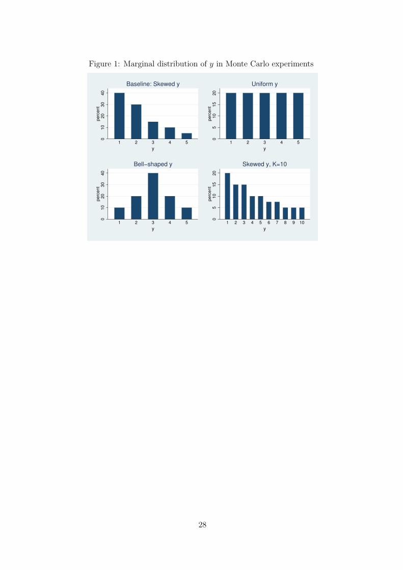
Figure 1: Marginal distribution of y in Monte Carlo experiments
01
02
03
04
0p
erc
en
t
1 2 3 4 5
y
Baseline: Skewed y
05
10
15
20
pe
rce
nt
1 2 3 4 5
y
Uniform y
01
02
03
04
0p
erc
en
t
1 2 3 4 5
y
Bell−shaped y
05
10
15
20
pe
rce
nt
1 2 3 4 5 6 7 8 9 10
y
Skewed y, K=10
28
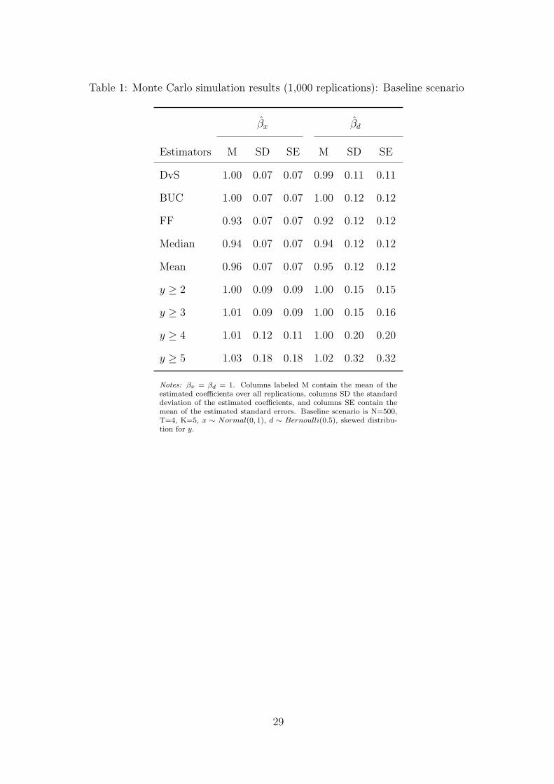
Table 1: Monte Carlo simulation results (1,000 replications): Baseline scenario
βx βd
Estimators M SD SE M SD SE
DvS 1.00 0.07 0.07 0.99 0.11 0.11
BUC 1.00 0.07 0.07 1.00 0.12 0.12
FF 0.93 0.07 0.07 0.92 0.12 0.12
Median 0.94 0.07 0.07 0.94 0.12 0.12
Mean 0.96 0.07 0.07 0.95 0.12 0.12
y ≥ 2 1.00 0.09 0.09 1.00 0.15 0.15
y ≥ 3 1.01 0.09 0.09 1.00 0.15 0.16
y ≥ 4 1.01 0.12 0.11 1.00 0.20 0.20
y ≥ 5 1.03 0.18 0.18 1.02 0.32 0.32
Notes: βx = βd = 1. Columns labeled M contain the mean of theestimated coefficients over all replications, columns SD the standarddeviation of the estimated coefficients, and columns SE contain themean of the estimated standard errors. Baseline scenario is N=500,T=4, K=5, x ∼ Normal(0, 1), d ∼ Bernoulli(0.5), skewed distribu-tion for y.
29
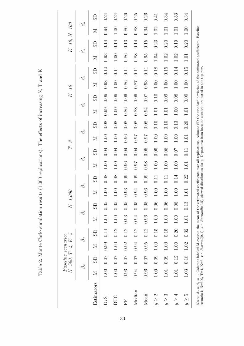
Tab
le2:
Mon
teC
arlo
sim
ula
tion
resu
lts
(1,0
00re
plica
tion
s):
The
effec
tsof
incr
easi
ng
N,
Tan
dK
Bas
elin
esc
enar
io:
N=
500,
T=
4,K
=5
N=
1,00
0T
=8
K=
10K
=10
,N
=10
0
βx
βd
βx
βd
βx
βd
βx
βd
βx
βd
Est
imat
ors
MSD
MSD
MSD
MSD
MSD
MSD
MSD
MSD
MSD
MSD
DvS
1.00
0.07
0.99
0.11
1.00
0.05
1.00
0.08
1.00
0.04
1.00
0.08
0.99
0.06
0.98
0.10
0.93
0.14
0.94
0.24
BU
C1.
000.
071.
000.
121.
000.
051.
000.
081.
000.
041.
000.
081.
000.
061.
000.
111.
000.
141.
000.
24
FF
0.93
0.07
0.92
0.12
0.93
0.05
0.93
0.09
0.96
0.04
0.96
0.08
0.86
0.06
0.86
0.11
0.86
0.13
0.86
0.26
Med
ian
0.94
0.07
0.94
0.12
0.94
0.05
0.94
0.09
0.97
0.04
0.97
0.08
0.88
0.06
0.87
0.11
0.88
0.14
0.88
0.25
Mea
n0.
960.
070.
950.
120.
960.
050.
960.
090.
980.
050.
970.
080.
940.
070.
930.
110.
950.
150.
940.
26
y≥
21.
000.
091.
000.
151.
000.
061.
000.
111.
000.
051.
000.
101.
010.
101.
000.
181.
040.
231.
020.
41
y≥
31.
010.
091.
000.
151.
000.
061.
000.
111.
000.
061.
000.
101.
010.
091.
000.
151.
020.
201.
010.
34
y≥
41.
010.
121.
000.
201.
000.
081.
000.
141.
000.
071.
000.
131.
000.
081.
000.
141.
020.
191.
010.
33
y≥
51.
030.
181.
020.
321.
010.
131.
010.
221.
010.
111.
010.
201.
010.
091.
000.
151.
010.
201.
000.
34
Note
s:β
x=β
d=
1.
Colu
mn
sla
bel
edM
conta
inth
em
ean
of
the
esti
mate
dco
effici
ents
over
all
rep
lica
tion
s,co
lum
ns
SD
the
stan
dard
dev
iati
on
of
the
esti
mate
dco
effici
ents
.B
ase
lin
esc
enari
ois
N=
500,
T=
4,
K=
5,x∼Normal(
0,1
),d∼Bernoulli(
0.5
),sk
ewed
dis
trib
uti
on
fory.
Dep
art
ure
sfr
om
base
lin
esc
enari
oare
note
din
the
top
row
.
30
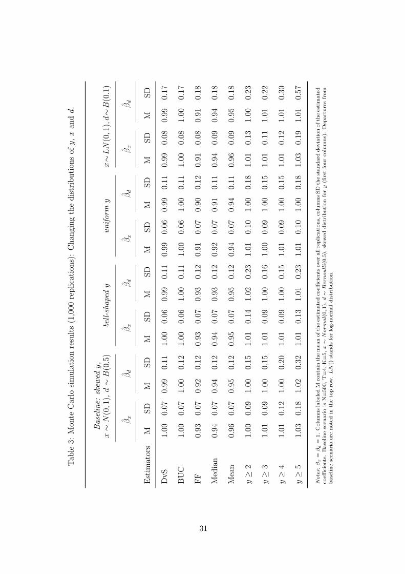
Tab
le3:
Mon
teC
arlo
sim
ula
tion
resu
lts
(1,0
00re
plica
tion
s):
Chan
ging
the
dis
trib
uti
ons
ofy,x
andd.
Bas
elin
e:sk
ewedy
,x∼N
(0,1
),d∼B
(0.5
)be
ll-s
hape
dy
un
ifor
my
x∼LN
(0,1
),d∼B
(0.1
)
βx
βd
βx
βd
βx
βd
βx
βd
Est
imat
ors
MSD
MSD
MSD
MSD
MSD
MSD
MSD
MSD
DvS
1.00
0.07
0.99
0.11
1.00
0.06
0.99
0.11
0.99
0.06
0.99
0.11
0.99
0.08
0.99
0.17
BU
C1.
000.
071.
000.
121.
000.
061.
000.
111.
000.
061.
000.
111.
000.
081.
000.
17
FF
0.93
0.07
0.92
0.12
0.93
0.07
0.93
0.12
0.91
0.07
0.90
0.12
0.91
0.08
0.91
0.18
Med
ian
0.94
0.07
0.94
0.12
0.94
0.07
0.93
0.12
0.92
0.07
0.91
0.11
0.94
0.09
0.94
0.18
Mea
n0.
960.
070.
950.
120.
950.
070.
950.
120.
940.
070.
940.
110.
960.
090.
950.
18
y≥
21.
000.
091.
000.
151.
010.
141.
020.
231.
010.
101.
000.
181.
010.
131.
000.
23
y≥
31.
010.
091.
000.
151.
010.
091.
000.
161.
000.
091.
000.
151.
010.
111.
010.
22
y≥
41.
010.
121.
000.
201.
010.
091.
000.
151.
010.
091.
000.
151.
010.
121.
010.
30
y≥
51.
030.
181.
020.
321.
010.
131.
010.
231.
010.
101.
000.
181.
030.
191.
010.
57
Note
s:β
x=β
d=
1.
Colu
mn
sla
bel
edM
conta
inth
em
ean
ofth
ees
tim
ate
dco
effici
ents
over
all
rep
lica
tion
s,co
lum
ns
SD
the
stan
dard
dev
iati
on
ofth
ees
tim
ate
dco
effici
ents
.B
ase
lin
esc
enari
ois
N=
500,
T=
4,
K=
5,x∼Normal(
0,1
),d∼Bernoulli(
0.5
),sk
ewed
dis
trib
uti
on
fory
(firs
tfo
ur
colu
mn
s).
Dep
art
ure
sfr
om
base
lin
esc
enari
oare
note
din
the
top
row
.LN
()st
an
ds
for
log-n
orm
al
dis
trib
uti
on
.
31
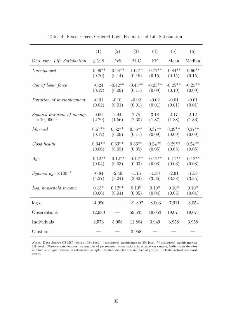
Table 4: Fixed Effects Ordered Logit Estimates of Life Satisfaction
(1) (2) (3) (4) (5) (6)
Dep. var.: Life Satisfaction y ≥ 8 DvS BUC FF Mean Median
Unemployed -0.96** -0.98** -1.03** -0.77** -0.84** -0.66**(0.20) (0.14) (0.16) (0.15) (0.15) (0.15)
Out of labor force -0.24 -0.42** -0.45** -0.25** -0.25** -0.25**(0.12) (0.09) (0.11) (0.09) (0.10) (0.09)
Duration of unemployment -0.01 -0.01 -0.02 -0.02 -0.01 -0.01(0.02) (0.01) (0.01) (0.01) (0.01) (0.01)
Squared duration of unemp. 0.60 2.44 2.75 3.18 2.17 2.12×10, 000−1 (2.79) (1.56) (2.30) (1.87) (1.88) (1.86)
Married 0.67** 0.52** 0.56** 0.37** 0.39** 0.37**(0.12) (0.09) (0.11) (0.09) (0.09) (0.09)
Good health 0.34** 0.33** 0.36** 0.24** 0.29** 0.24**(0.06) (0.05) (0.05) (0.05) (0.05) (0.05)
Age -0.12** -0.12** -0.12** -0.12** -0.11** -0.12**(0.04) (0.03) (0.03) (0.03) (0.03) (0.03)
Squared age ×100−1 -0.84 -2.46 -1.15 -1.30 -2.91 -1.58(4.27) (3.24) (3.82) (3.36) (3.38) (3.35)
Log. household income 0.13* 0.12** 0.13* 0.10* 0.10* 0.10*(0.06) (0.04) (0.05) (0.04) (0.05) (0.04)
logL -4,996 — -21,802 -8,003 -7,911 -8,054
Observations 12,980 — 59,535 19,053 19,071 19,071
Individuals 2,573 3,958 11,864 3,949 3,958 3,958
Clusters — — 3,958 — — —
Notes: Data Source GSOEP, waves 1984-1989. * statistical significance at 5% level, ** statistical significance at1% level. Observations denotes the number of person-year observations in estimation sample; Individuals denotesnumber of unique persons in estimation sample; Clusters denotes the number of groups in cluster-robust standarderrors.
32