consistent model specification tests: omitted variables
TRANSCRIPT
Consistent Model Specification Tests: Omitted Variables and Semiparametric Functional FormsAuthor(s): Yanqin Fan and Qi LiSource: Econometrica, Vol. 64, No. 4 (Jul., 1996), pp. 865-890Published by: The Econometric SocietyStable URL: http://www.jstor.org/stable/2171848 .
Accessed: 30/04/2013 14:21
Your use of the JSTOR archive indicates your acceptance of the Terms & Conditions of Use, available at .http://www.jstor.org/page/info/about/policies/terms.jsp
.JSTOR is a not-for-profit service that helps scholars, researchers, and students discover, use, and build upon a wide range ofcontent in a trusted digital archive. We use information technology and tools to increase productivity and facilitate new formsof scholarship. For more information about JSTOR, please contact [email protected].
.
The Econometric Society is collaborating with JSTOR to digitize, preserve and extend access to Econometrica.
http://www.jstor.org
This content downloaded from 128.194.113.59 on Tue, 30 Apr 2013 14:21:17 PMAll use subject to JSTOR Terms and Conditions

Econometrica, Vol. 64, No.4 (July, 1996), 865-890
CONSISTENT MODEL SPECIFICATION TESTS: OMITTED VARIABLES AND SEMIPARAMETRIC FUNCTIONAL FORMS
BY YANQIN FAN AND Qi LI1
In this paper, we develop several consistent tests in the context of a nonparametric regression model. These include tests for the significance of a subset of regressors and tests for the specification of the semiparametric functional form of the regression function, where the latter covers tests for a partially linear and a single index specification against a general nonparametric alternative. One common feature to the construction of all these tests is the use of the Central Limit Theorem for degenerate U-statistics of order higher than two. As a result, they share the same advantages over most of the correspond- ing existing tests in the literature: (a) They do not depend on any ad hoc modifications such as sample splitting, random weighting, etc. (b) Under the alternative hypotheses, the test statistics in this paper diverge to positive infinity at a faster rate than those based on ad hoc modifications.
KEYWORDS: Consistent tests, degenerate U-statistics, kernel estimation, omitted variables, partially linear model, single index model.
1. INTRODUCTION
RECENTLY, NONPARAMETRIC FUNCTIONAL ESTIMATION TECHNIQUES such as kernel and series methods have been used to construct consistent model specification tests.2 These include tests for a parametric model versus a nonparametric model, tests for the significance of a subset of regressors in a nonparametric regression model, and tests for a semiparametric (partially linear or single index) model against a nonparametric altemative. For example, Fan and Li (1992a), Hardle and Mammen (1993), Hidalgo (1992), and Lee (1994) have developed consistent tests for a parametric specification by using the kernel regression estimation technique; Eubank and Spiegelman (1990), Hong and White (1995), and Wooldridge (1992) have applied the method of series estimation to consist- ent testing for a parametric regression model; consistent tests for omitted variables were considered by Hidalgo (1992) and Gozalo (1993), among others; Lavergne and Vuong (1996) proposed a method to select between two sets of regressors using kernel estimators; Whang and Andrews (1993) and Yatchew (1992) have developed consistent tests for a partially linear model versus a
1 The first author would like to thank the Natural Sciences and Engineering Research Council and the Social Sciences and Humanities Research Council of Canada for their support and the second author would like to acknowledge the Social Sciences and Humanities Research Council of Canada for its support.
2 Bierens (1982) was the first to give a consistent conditional moment model specification test; see also Bierens (1990), Bierens and Ploberger (1994), and references therein. Using nonparametric estimation technique to construct consistent model specification tests was first suggested by Ullah (1985). Robinson (1989) was the first to propose some nonparametric tests for time-series models.
865
This content downloaded from 128.194.113.59 on Tue, 30 Apr 2013 14:21:17 PMAll use subject to JSTOR Terms and Conditions

866 YANQIN FAN AND QI LI
nonparametric alternative; consistent tests for a single index specification have been presented in Chen (1992) and Rodriguez and Stoker (1992).
The first group of papers that make use of nonparametric estimation tech- niques in developing consistent tests for a parametric functional form such as Hidalgo (1992), Lee (1994), and Wooldridge (1992) among others have employed ad hoc modifications such as sample splitting or a form of weighting. Recently a number of authors have successfully used the Central Limit Theorems (CLTs) for second order degenerate U-statistics in Hall (1984) and De Jong (1987) to develop some consistent nonparametric tests for a parametric density function or a parametric regression function; see, e.g., Eubank and Hart (1992), Fan (1994), Fan and Li (1992a, b), Hardle and Mammon (1993), Hong and White (1995), Horowitz and Hardle (1994), and Li (1994), to mention only a few. However to the best of our knowledge, the existing consistent tests for a semiparametric functional form such as a partially linear model or a single index model and tests for omitted variables in a nonparametric model still employ ad hoc modifications. For example, for testing a partially linear model versus a nonparametric regression model, Whang and Andrews (1993) and Yatchew (1992) used sample splitting; for testing a single index model, Chen (1992) used sample splitting, and Rodriguez and Stoker (1992) introduced a test statistic that has a degenerate limiting distribution under the null hypothesis; for testing omitted variables, Robinson (1991) discussed the application of a form of nonstochastic weighting which is equivalent to a form of sample splitting, Hidalgo (1992) introduced random weighting, and Gozalo (1993) used a random search procedure.3 These ad hoc modifications are introduced in the aforemen- tioned studies in order to overcome the so called "degeneracy problem": an appropriate estimator of some measure of the distance between the models to be tested under the null hypothesis approaches zero at a rate faster than n -1/2,
where n is the sample size. As a consequence, when normalized by n /2, the estimator of the chosen measure does not have a well-defined limiting distribu- tion under the null hypothesis. This degeneracy problem is caused by the fact that the estimator of the chosen measure contains in its expression some degenerate U-statistic which vanishes at a rate faster than n 1/2. Without modifying this estimator, its asymptotic distribution under the null hypothesis would be determined by the degenerate U-statistic. In the papers we just cited, ad hoc modifications are employed such that the asymptotic distribution of the estimator of the chosen measure in each of these papers is determined by a random term that is of a larger order than the corresponding U-statistic. However, rather than introducing ad hoc methods to avoid the degeneracy problem, it seems natural, as in recent papers on consistent tests for a paramet- ric functional form mentioned earlier, to exploit this special property by invok- ing the CLTs for degenerate U-statistics (of order possibly higher than two) to
3Recently Lavergne and Vuong (1996) constructed a nonparametric test for selecting regressors. They require that the competing sets of regressors be non-nested. Hence their test is different from the usual omitted variables test.
This content downloaded from 128.194.113.59 on Tue, 30 Apr 2013 14:21:17 PMAll use subject to JSTOR Terms and Conditions
CONSISTENT MODEL SPECIFICATION TESTS 867
develop consistent tests for omitted variables and for semiparametric functional forms. This forms the core of the present paper. Tests that exploit this special property may also be more powerful than those based on ad hoc modifications,4 because under the alternative hypothesis the corresponding test statistics di- verge to + oo at a rate faster than nl/2.
The remainder of this paper is organized as follows. We introduce the nonparametric regression model and the hypotheses to be tested in Section 2. Section 3 constructs a consistent test for omitted variables in the context of the nonparametric regression model introduced in Section 2. Section 4 presents respectively a consistent test for a partially linear specification and a consistent test for a single index specification of the regression function. The last section concludes and offers some suggestions for further research. Appendix A con- tains proofs of the main results in Sections 3 and 4. Appendix B contains some technical lemmas that are used in the proofs of Appendix A. In particular, it contains an extension of the CLT in Hall (1984) for degenerate U-statistics of second order to degenerate U-statistics of any finite order. This is useful because the test statistics to be constructed in this paper involve degenerate U-statistics of order higher than two.
Throughout the rest of this paper, all the limits are taken as n -* oo. Ej i= EJ% 1,Ej * i = E% i,j= 1, etc.
2. THE MODEL AND THE HYPOTHESES
Consider the nonparametric regression model:
(1) Yi =g(Xd + Ei,
where {Yi, X}in1 is a set of n independent and identically distributed (i.i.d.) observations on {Y, X'}' with Y the scalar dependent variable and X the d x 1 regressors, g(.): Rd-* R is the true, but unknown regression function, and e1 is the error satisfying E[ ei I Xi ] = O.
Two classes of hypotheses that are often tested concerning the regression model (1) are the functional form of g( ) and the significance of a subset of regressors X. With respect to the functional form of g, the null hypothesis specifies either a parametric regression model or a semiparametric regression model for g( ). As motivated in Section 1, we will focus on the null hypothesis of a semiparametric regression model in this paper.
We first present the problem of testing for the significance of a subset of regressors. Let Xi = (Wi', Z)', where Wi is of dimension q1 x 1 andZi is of dimension q2 x 1, q1 + q2 = d. Then, a subset of regressors, Zi (say), is insignifi- cant to the explanation of Yi given Wi if E[Yi Xi] = E[Yi Wi]. Insignificant regressors should be omitted from the regression model. Thus, a test of
4 See the last section for more discussion on this issue.
This content downloaded from 128.194.113.59 on Tue, 30 Apr 2013 14:21:17 PMAll use subject to JSTOR Terms and Conditions
868 YANQIN FAN AND QI LI
significance is also called an omitted variables test. Let r(w) = E[Yi I i = w]. Then an omitted variables test is that of
Ho: g(x) = r(w) a.e. against the general alternative
Ha: g(x) r(w),
where x = (w', z')' is partitioned according to that of Xi. Since Robinson (1988) and Powell, Stock, and Stoker (1989), partially linear
and single index models have attracted much attention among econometricians,5 because on one hand, these models are not as restrictive as parametric regres- sion models and on the other hand, they alleviate the problem of the "curse of dimensionality" associated with nonparametric models. However, they are still not free from misspecification errors. Thus, it is important to test the validity of such semiparametric models against the general nonparametric alternative. The first attempt toward developing consistent tests of these semiparametric models has been made by Whang and Andrews (1993) and Yatchew (1992) for partially linear regression models, and by Chen (1992) and Rodriguez and Stoker (1992) for single index models. As mentioned in Section 1, these tests used some kind of ad hoc modifications (such as sample splitting) to avoid direct treatment of degenerate U-statistics. Sample splitting results in inefficient estimators. It may also cause the tests to lose power both directly and indirectly. The indirect effect of sample splitting on these tests is to slow down the divergence rate of the test statistics to + oo. This motivates us to develop consistent tests for a partially linear model and for a single index model that make use of the special feature of degenerate U-statistics.
For a partially linear model, the null hypothesis is
Hb: g(x) =z'y+ 0(w) a.e.
for some y ERq2 and some 0( ): Rql -R,
and the alternative is
Hb: g(x) Z'y+ ' 0(w) for all y E Rq2 and all 0( ): Rql -*R,
where as before, x = (w', z')'. Finally for a single index model, the null hypothesis is
Ho: g(x) = (a ( 'x) a.e. for some a E Rd and some p( ): R -R ,
and the alternative is
Hc: g(x) p (a ( 'x) for all a E Rd and all (p(.): R -R.
SSee Engle, et al. (1986), Hardle and Stoker (1989), Stock (1989), and Stoker (1992) for empirical applications of partially linear and index models.
This content downloaded from 128.194.113.59 on Tue, 30 Apr 2013 14:21:17 PMAll use subject to JSTOR Terms and Conditions
CONSISTENT MODEL SPECIFICATION TESTS 869
3. A CONSISTENT TEST FOR OMITTED VARLIBLES
Recall from Section 2 that under the null hypothesis Ho: g(Xi) = r(W), a.e., where Xi = (W1', Z')'. Let ui = Yi - r(W). Then under the null hypothesis, the regression model becomes
(2) Yi = r(W) + ui,
where E(ui I Xi) = g(Xi) - r(W) = 0 under Ho and E(ui I Xi) # 0 under H'. Observing that E[uiE(ui I Xi)] = E{[E(ui I Xi)]2} > 0 and the equality
holds if and only if Ho is true, we can construct a consistent test6 based on E[ uiE(ui I Xi)]. If ui and E(ui I Xi) were available, then we could estimate E[tuiE(ui I Xi)] by its sample analogue: n-1 Ei uiE(ui IXi). To get a feasible test statistic, we need to estimate ui by the corresponding residual from (2) and E(ui I Xi) by an appropriate kernel estimator. To overcome the random denomi- nator problem in the kernel estimation, we choose to estimate a density weighted version of n-1 Ej uiE(u1 IXj) given by n-1 Ej[ujfw.]E[ujfw, IXj]f(Xj), where fw, =fw(Wi), fw() is the probability density function (p.d.f.) of Wi, and f(-) is the p.d.f. of Xi.
Specifically, we estimate u1 by i = (Y1- i): the nonparametric residual from (2), where Yi is a kernel estimator of r(W) defined as
A3 R [n - 1)aq, ] -1 Ej ,i YjKiw:
fw
and fw. is the corresponding kernel estimator of fw, given by
(4) tw )qE K.wj,, J*i
where K!W = KW((Wi - Wj)/a) with Kw0) being a product-kernel formed from the univariate kernel kw(-) and a an a smoothing parameter. We estimate
E[ifw, I Xi ]f(Xi) by [(n - )hd ijfwj where
K1 =K(ih i)=K( h ihj,
K is a product kernel with univariate kernel function k(-), and h hn is a smoothing parameter.
6 This test can be regarded as a generalized conditional moment test of omitted variables, where the weight function is a nonparametric function given by E(ui IXi =x). See Newey (1985) and Tauchen (1985) for the conditional moment tests of functional forms based on a finite number of parametric weight functions.
This content downloaded from 128.194.113.59 on Tue, 30 Apr 2013 14:21:17 PMAll use subject to JSTOR Terms and Conditions

870 YANQIN FAN AND QI LI
Our test statistic will be based on
def 1 1 AJ~1
(6) a = ii = (- Ki-
r1 = r(W), rI and u2 are defined in the same way as Y in (3) with Y replaced by r(W;) and Uj respectively.
To derive the asymptotic distribution of I,a under Ho, we will use the following definitions (see Robinson (1988)) and assumptions.
DEFINITION 1: X, I 2 1, is the class of even functions k: R -*R satisfying
R
k(u) = O((i + IuIl+1+e)')j some e>0,
where b is the Kronecker's delta.
DEFINITION 2: ,], aE> 0, ,U >O0, is the class of functions g: Rd -*R satisfy- ing: g is (m - 1)-times partially differentiable, for m - 1 ? ,u ? m; for some Pw> 0, for all z, where {y: Iy - zI < p}; Qg = 0 when m = 1; Qg is a (m - 1)th degree homogeneous polynomial in y - z with coefficients the partial derivatives of g at z of orders 1 through m - 1 when m > 1; and g(z), its partial derivatives of order m - 1 and less, and h g(z), have finite atth moments.
Assumption A
(A1) (a) fe=
for some A>0 andr e for some ,u >0; (b) kW E++m1
for integers land msuch thatl- 1 < A?<land m -1 < ,u<m; (c) f e , keZ; (d) The error E = Y - g(X) satisfies E 1 e4 1 < . The conditional variance function
r =2(x) =W EaXn=dx] and m4(x) iE[e4IX=x] are continuous. In addition, f(x)a2(x) and f(x)m4(x) are bounded on Rd.
(A2) As n -oo, a-*0, a the c, of evoo nhdction, na2khd/2* > O and hd/a2q1 0, where q1 = min(A + 1,K ,).
This content downloaded from 128.194.113.59 on Tue, 30 Apr 2013 14:21:17 PMAll use subject to JSTOR Terms and Conditions
CONSISTENT MODEL SPECIFICATION TESTS 871
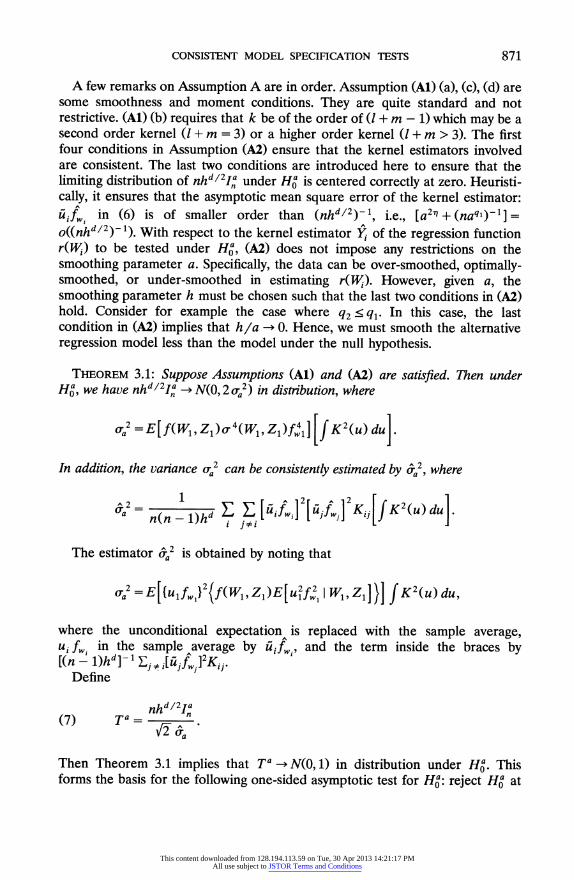
A few remarks on Assumption A are in order. Assumption (Al) (a), (c), (d) are some smoothness and moment conditions. They are quite standard and not restrictive. (Al) (b) requires that k be of the order of (1 + m - 1) which may be a second order kernel (1 + m = 3) or a higher order kernel (1 + m > 3). The first four conditions in Assumption (A2) ensure that the kernel estimators involved are consistent. The last two conditions are introduced here to ensure that the limiting distribution of nhd/2IJ, under H' is centered correctly at zero. Heuristi- cally, it ensures that the asymptotic mean square error of the kernel estimator: uifw in (6) is of smaller order than (nhd/2)-l, i.e., [a2 + (naqi)-'] -
o((nhd/2)-1). With respect to the kernel estimator Yi of the regression function r(W) to be tested under Hoa, (A2) does not impose any restrictions on the smoothing parameter a. Specifically, the data can be over-smoothed, optimally- smoothed, or under-smoothed in estimating r(W). However, given a, the smoothing parameter h must be chosen such that the last two conditions in (A2) hold. Consider for example the case where q2 ?q1. In this case, the last condition in (A2) implies that h/a -O0. Hence, we must smooth the alternative regression model less than the model under the null hypothesis.
THEOREM 3.1: Suppose Assumptions (Al) and (AS) are satisfied. Then under Hog, we have nhd/2I,a > N(0, 2 o.2) in distribution, where
2 =E[T x,'Z)4(WT, Zl)f\41 [ 2(U) du]. 0a = (,9Z)o
In addition, the vartiance a can be consistently estimated by Ca2 where
52 n(n- 1)hd E[iiifwi] [ljfwjI Kij[fK2(u)dul. i j5o1
The estimator 6 2 is obtained by noting that
a2=E{UlfwJ12 { tW lE u 2w2 1 Zlg K }]|2(U) du, 0a= E[{f2f(W9Zl)E[u2f21 W 1\
where the unconditional expectation is replaced with the sample average, uifw in the sample average by [ifw, and the term inside the braces by [(n - l)h ]1 i[u fwj Kij.
Define
nhd/2I,a (7) T a=
Then Theorem 3.1 implies that Ta -+ N(O, 1) in distribution under Ho. This forms the basis for the following one-sided asymptotic test for Hoa: reject Hoa at
This content downloaded from 128.194.113.59 on Tue, 30 Apr 2013 14:21:17 PMAll use subject to JSTOR Terms and Conditions

872 YANQIN FAN AND QI LI
significance level ao if T' > Zao, where Zao is the upper ao-percentile of the standard normal distribution.
The consistency of this test is the last result of this section.
THEOREM 3.2: Assume (Al) and (A2) hold. Then the above test is consistent. In addition P(Ta > Mn I Ha) -> 1, where Mn is any positive, nonstochastic sequence with Mn = o((nhd/2)).
Theorem 3.2 follows from the facts that under Ha, Ia - E{f(X)[g(X) -
r(W)]2f 2(W)}(> 0) in probability and A6 = Op(1). The proofs of these are straightforward and are thus omitted.
4. CONSISTENT TESTS FOR SEMIPARAMETRIC MODELS
4.1. A Consistent Test ForA Partially Linear Model
Let vi = Yi- Z' - O(W). Then E(vi I Xi) = g(Xi) - [Z y + 0(W)] which equals zero a.e. if and only if the null hypothesis Hob is true. Hence, E[viE(vi IXi)] = E{[E(vi IXi)]2} ? 0 and the equality holds if and only if Hob holds. Thus, as in Section 3, we will base our test for Ho on an estimator of n1 i[vifwjE[vjfw, IXj]f(Xj) to overcome the random denominator problem in kernel estimation.
The estimator of vifw, that we adopt is obtained by a two-step procedure as in Robinson (1988) and Fan, Li, and Stengos (1995). In the first step, we estimate y by A defined as (see Fan, Li, and Stengos (1995) for more details)
(8) Z' S(2)fS(z )f(Y-)f,
where as in Robinson (1988), SAfW, Bfl = nl Ei Aifw Bifw, and SAfW = SAfW, AW
for scalar or column vectors Aifwi and Bifwi. In addition, Zi =
[(n - 1)ai Ej ZjK1KJ/fw, estimates E[Zi W], f W and Yi are defined in (3) and (4) respectively. Let -vi = (Yi - 1) - (Zi - Zi)'9. Then, the density- weighted error vifwl is estimated by
(9) fwi= -Yi fw-(z z Wi- (Zi - ( y- fw
= [(a-a) +vi- ifwi- i-) (e- )fwi
=Difwi - zi-i (e- fwi9
where O 9 = 0(Wa), Oand vi are defined as in (3) with Yi replaced by 0(Wj) and v def(oi A)+vi _A respectively, and i3 = oj - )+ Vi 3.
This content downloaded from 128.194.113.59 on Tue, 30 Apr 2013 14:21:17 PMAll use subject to JSTOR Terms and Conditions
CONSISTENT MODEL SPECIFICATION TESTS 873
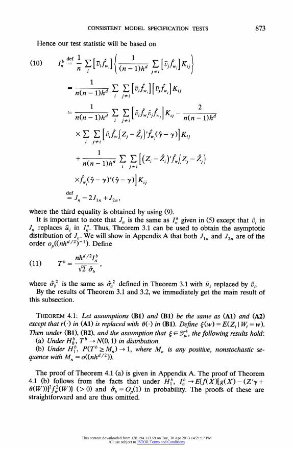
Hence our test statistic will be based on
(10) In n EI n ifw{ En [ fwjI K)
1~~~~~~*
n(n-l)hd ~ ~ ~ !~ E Vt][UfKij
n(n - l)hd - fw n(n-)hd
i j5i
i j#i
n(n - 1)hd Z E [(z,-i fW(zj -Z)
XW (Ae- )'(A y)] Kij
def Jn 2Jin +J2n,
where the third equality is obtained by using (9). It is important to note that Jn is the same as In' given in (5) except that ui in
Jn replaces ui in In,. Thus, Theorem 3.1 can be used to obtain the asymptotic distribution of Jn. We will show in Appendix A that both J1, and J2n are of the order o ((nhd/2)-l). Define
nhd/21b (11) Tb = n
V'ab
where &b2 is the same as Ca2 defined in Theorem 3.1 with ui replaced by vi. By the results of Theorem 3.1 and 3.2, we immediately get the main result of
this subsection.
THEOREM 4.1: Let assumptions (Bi) and (Bi) be the same as (Al) and (A2) except that r(*) in (Al) is replaced with 0(0) in (Bi). Define (w) = E(Za I W = w). Then under (Bi), (B2), and the assumption that ( e -, the following results hold:
(a) Under Hob, Tb _ N(0, 1) in distribution. (b) Under Hi', P(Tb ? M- ) 1, where Mn is any positive, nonstochastic se-
quence with Mn - o((nhd/2)).
The proof of Theorem 4.1 (a) is given in Appendix A. The proof of Theorem 4.1 (b) follows from the facts that under H, Ib b -* E{f(X)[g(X) - (Z'y + O(W))]2f 2(W)} (>0) and b = Op(1) in probability. The proofs of these are straightforward and are thus omitted.
This content downloaded from 128.194.113.59 on Tue, 30 Apr 2013 14:21:17 PMAll use subject to JSTOR Terms and Conditions

874 YANQIN FAN AND QI LI
4.2. A Consistent Test ForA Single Index Model
The test for Ho versus H' is constructed in a similar way to that for Hob versus Hi . Specifically, define vi=Yi -(a'Xi). Then a consistent test for Ho versus Hf can be based on an appropriate estimator of E[vifa(a'Xi)E{vifa(a'Xi)lXi}f(Xi)], where fa(-) is the density function of a 'Xi.
Let a' be the density-weighted average derivative estimator proposed by Powell, Stock, and Stoker (1989).7 We assume that the conditions in Powell, Stock, and Stoker (1989) hold under Ho. Hence, a' - a = O(n'/2). Under Ho' the index function p( a'Xi) can be consistently estimated by
(12) AY1Il'X )= [(n - 1)ha Ei YjKia fa(&A'Xi)
where Ka) = k((& 'X, - & 'Xj)/ha) with kaQ) a univariate kernel function, ha is a smoothing parameter, and
(13) fa(atX) a2 K (n-1)ha o
Let vi = a- AYi I 'Xi). Then our test will be based on
(14) n n E a( a (n -)h E v, fa a Ki1}
n(n -1 E E [ Vifa ( j)] [fa a 'x )]Kij. i j1oi
It follows from (12) and (13) that (15) Via ( At Xi) =[ Yi-(Yi l fXi)] fa (c i (15) vijfa(&a j)Y E ( a&'j)fa(&Xa
= (n -1)h (Yi j
= [-(Yi I a'Xi)] fa (a 'Xi)
+ n- iYj ) [ K& iK a ] 1
fna (n1 - 1)h[KJ -K1i 'fl 1)ha j a ji = vifa ( asXi) + n-)hE( iY)[ iK j]
where E(Yi a a'Xi) and fa(a' Xi) are defined respectively in (12) and (13) with a replaced by ac, vi is the residual from kernel estimation of Yi = (c(a'Xi) + vi,
7For the asymptotic theory for average derivatives in time series context, see Robinson (1989). Robinson (1989) and Stoker (1989) are the first papers using average derivatives in hypothesis testing.
This content downloaded from 128.194.113.59 on Tue, 30 Apr 2013 14:21:17 PMAll use subject to JSTOR Terms and Conditions
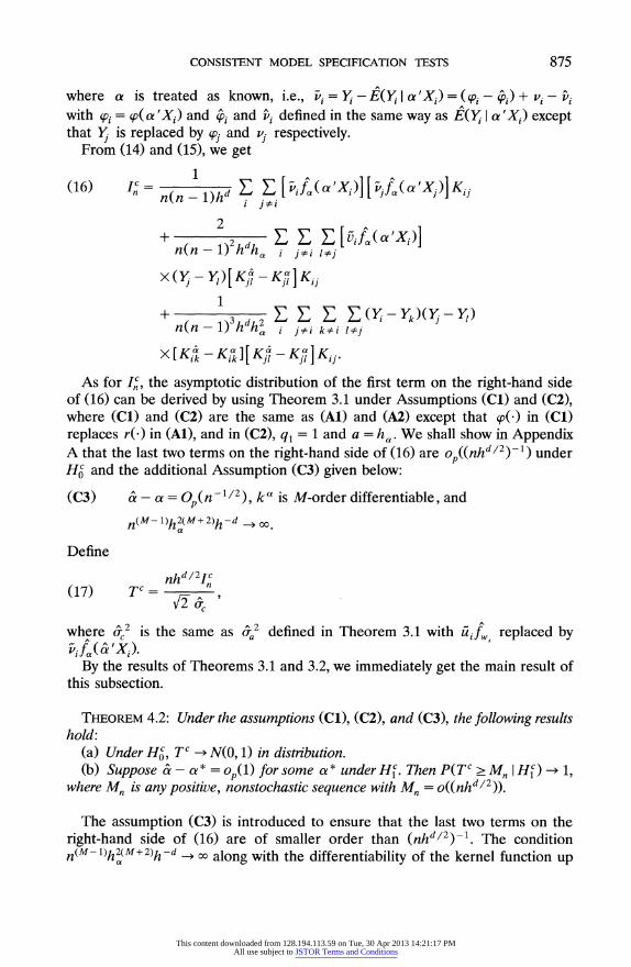
CONSISTENT MODEL SPECIFICATION TESTS 875
where a is treated as known, i.e., i = Y iI 'Xi) Pi vi vi with (pi = qp(a'Xj) and (pi and vi defined in the same way as E(Y I a'Xi) except that Yj is replaced by (pj and vj respectively.
From (14) and (15), we get
(16) n(n-1)hd E f[ai (f( Xi)]K[ijfa(a'Xi)]K i ji/i
2 + D(n1)hdh E E E[iif(a'Xi)]
xY- Y1)[KJ -K1Jl Ki1
1 + 3 (Y - Yk)(y- Yl)
n(n-1) h dh, j?i k?i i?]
X [Klk- Ka] [ Kl - Kjl ] Kij.
As for Inc, the asymptotic distribution of the first term on the right-hand side of (16) can be derived by using Theorem 3.1 under Assumptions (Cl) and (C2), where (Cl) and (C2) are the same as (Al) and (A2) except that 'p0-) in (Cl) replaces r( ) in (Al), and in (C2), q1 = 1 and a = ha- We shall show in Appendix A that the last two terms on the right-hand side of (16) are op((nhd/2)-l) under Hoc and the additional Assumption (C3) given below:
(C3) a - a = O (n -2), k is M-order differentiable, and
n(M- 1)h2(M+ 2)h -d 00
a
Define
nhd/2I,c (17) Tc=
where (J2 is the same as o)a defined in Theorem 3.1 with iifW replaced by vfa( ^Xd)
By the results of Theorems 3.1 and 3.2, we immediately get the main result of this subsection.
THEOREM 4.2: Under the assumptions (Cl), (C2), and (C3), the following results hold:
(a) Under Hoc, Tc - N(O, 1) in distribution. (b) Suppose a -^a * = op(1) for some a * under Hc. Then P(TC > Mn I HO) -> 1,
where Mn is any positive, nonstochastic sequence with Mn = o((nhd/2)).
The assumption (C3) is introduced to ensure that the last two terms on the right-hand side of (16) are of smaller order than (nhd/2)-1. The condition n(M -l)h2(M+ 2)h -d oo along with the differentiability of the kernel function up
This content downloaded from 128.194.113.59 on Tue, 30 Apr 2013 14:21:17 PMAll use subject to JSTOR Terms and Conditions

876 YANQIN FAN AND QI LI
to order M may be relaxed by using uniform convergence results for U-processes. However, the proof would become much more involved. Since the kernel function is chosen by the researcher, one can always choose a kernel function that has as many derivatives as possible so that the condition:
n(M - l)h2(M + 2)h -d o a
is satisfied for a wide range of values of ha and h.
5. CONCLUSIONS
We have proposed consistent tests for a partially linear regression model and an index model. In addition, we have developed a consistent test for omitted variables in a nonparametric regression model without specifying its functional form. These tests are constructed by invoking the CLT for degenerate U- statistics of order higher than two. As a result, they do not rely on any arbitrary modifications, and under the alternative hypotheses the test statistics diverge to + oo at a faster rate than nl/2.
Similar to the power analysis of consistent tests for a parametric functional form provided in Fan and Li (1992a), Hardle and Mammen (1993), one could also investigate the local power properties of the tests developed in this paper. Under some additional conditions, one can show that the tests proposed in this paper can detect sequences of local alternatives that differ from the respective null hypotheses by O((nhd/2)-1/2). Hence, they are more powerful than those based on arbitrary modifications, because the latter can only detect local alternatives distant apart from the respective null by O(n-l'/4). To the best of our knowledge, the tests proposed in this paper are the first consistent tests for a partially linear model, a single index model, and omitted variables that possess this desirable property.
Another issue that deserves some discussion is the support of X. In this paper, we have assumed that the support of X is the whole Euclidean space Rd. One could easily show that the tests in this paper are still valid if the support of X is a finite convex subset of Rd and the density function of X vanishes on the boundary of its support. However, if the support of X is a compact subset of Rd
and the density function of X is bounded away from zero on its support, then the tests presented in this paper need to be modified. In this case, some trimming method must be introduced to overcome the boundary effect. The simplest way of doing this is to introduce a fixed weight function such that the support of the weight is a proper subset of the support of X as in Fan and Li (1992b). However, the resulting tests will be consistent only against the alterna- tives that differ from the null on the support of the weight function. In order for the tests to be consistent against all the alternatives, the weight function must change with respect to the sample size in such a way that its support approaches the support of X as the sample size n goes to + oo.
This content downloaded from 128.194.113.59 on Tue, 30 Apr 2013 14:21:17 PMAll use subject to JSTOR Terms and Conditions

CONSISTENT MODEL SPECIFICATION TESTS 877
Department of Economics, University of Windsor, Windsor, Ontario, Canada, N9B 3P4
and Department of Economics, University of Guelph, Guelph, Ontario, Canada,
NIG 2W1
Manuscript received December, 1992; final revision received July, 1995.
APPENDIX A: PROOFS OF THE THEOREMS
This appendix collects proofs of the main results stated in Sections 3 and 4. Throughout, the symbol C denotes a generic constant. When we evaluate the order of some terms, if there is no confusion, we will use n, (n - 1), and (n - 2) interchangeably. In addition, when an expression contains more than one summation, by slight abuse of notation, we will sometimes use the same symbol to denote this expression and different terms in the expression obtained from restricting the summation indices to different cases. For example, if we define LA = Ei EY Aij, then we will also use LA to denote Ei Ej i Aij and Ej Aii corresponding to i #j and i =j respectively.
PROOF OF THEOREM 3.1: The following expression for I,, is immediate from (5) and (6):
(A.1) nnn_lhE (-ri fwi(rj ri) Vj + UiUjfw f" + fiif^ ufij^ (A.1) I ~ ---
Er'= '- (r - n(n - 1)jh ((1 ,),,1* ,f1
+ 2uifw (r. - P)f- 2j f,i(r? - 2ui)f f - 2uifw 'jfj}Kij
def - I, + I2 + I3 + 2I4 + 2I5 2I6.
We shall complete the proof of Theorem 3.1 by examining . I6 respectively in Propositions A.1 to A.6, and by showing that k 2 = 2+ op(1) in Proposition A.7. Since the proof is similar to that of Theorem 1 of Fan and Li (1992c), we will only provide some important steps here. Throughout this appendix, ij = (ui, Xi)' and Ei(-) = E( I Xi).
PROPOSITION A.1: I, = op((nh'/2) 1
PROOF: From (A.1), we get
(A.2) n(n-1)hd E E )fjKij
1 J#
n(n-1)hda2, E . 1: ,(ri r,)Kw(rj-rk)Kj"kvKij-. n(n - W)h da2q, i~ j 1#li k#j i
We will complete the proof by showing that E[(I)2] = o(n-2h-d). However a direct evaluation of E[(11)2] would be very tedious since it contains eight summations. Below we will first show that E(I) = o((nhd/2)-l). Then we will use this result and a symmetry argument to show that E[(I1)2 ] = o(n - 2h -d).
This content downloaded from 128.194.113.59 on Tue, 30 Apr 2013 14:21:17 PMAll use subject to JSTOR Terms and Conditions
878 YANQIN FAN AND QI LI
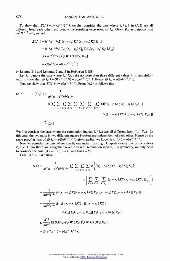
To show that E(I)=o((nhd/2)-l), we first consider the case where i,j,l,k in (A.2) are all different from each other and denote the resulting expression as Ill. Given the assumption that na277hd/2 -*0, we get
E(Ill) = h -d a - - r2)Kw(r -r4)K3wK13
= h-da -2qE{[Ej(rl-r2)Kw2][E3(r3 -r4)K3w]K13}
< Ch-da272E[Dr(Wi)Dr(W3)K13]
= O(a2,q) = o((nhd/2)-')
by Lemma B.1 and Lemmas 2 and 3 in Robinson (1988). Let 112 denote the case where i, j, 1, k take no more than three different values. It is straightfor-
ward to show that E(I12) = O(n-la -41) = o((nhd/2)-l ). Hence E(1) = o((nhd/2)-.
Now we show that E[(I1)2] = o(n -2h-d ). From (A.2), it follows that
(A.3) E[() (n-1) 2da4q
x E: E Y. E E E, E E, Et [(r - r ) K'l (r - rk )KJwk K,j i j?i l?i k?j i' j'?i' l'1i' k'*j'
X [(ri, - rl,)Kl(rj - rk,)Kr''k'Kij]}
def = LA3.
We first consider the case where the summation indices i, j, 1, k are all different from i', j', 1', k'. In this case, the two parts in two different square brackets are independent of each other. Hence by the same proof as that of E(I) = o((nhd/2)-1) given earlier, we know that LA3 =O(n-2h-d).
Next we consider the case where exactly one index from i, j, 1, k equals exactly one of the indices i', j', 1', k' (so there are altogether seven different summation indices). By symmetry, we only need to consider the case (i) i = i', (ii) i = I', and (iii) I = 1'.
Case (i) i = i': We have
LA3 = E E i E E [(ri - rl)Kw(rj - rk )Kjwk Kti] 2 1)6 2d 4qI j #jHi #
xl E E E(rirl,)lltri,rk')Ktk8KiiI ) n (n h a J*i 1*i'i l'?k k'?j
=-^ 9 E{(r1 - r3)Kw(r2
- r4)K2wK12[(r -r6)K1(rs-
r7)K
5K15]} 1
-h2dal E{[El(r1 - r3)KwL [E2(r2-r4)K?w]
XK12[El(r, -r6)K
-j[E (r5-r7)Kw]K15}
a4,q < n2 E{Dr(Wi)Dr(W2)Ki2Dr(Wi)Dr(W5)Ki5}
nh= l2Pr(WdDr=WdnKl5)
-O(a4 '7n -1) - O(n2h -d).
This content downloaded from 128.194.113.59 on Tue, 30 Apr 2013 14:21:17 PMAll use subject to JSTOR Terms and Conditions
CONSISTENT MODEL SPECIFICATION TESTS 879
For case (ii) i = 1', we have
1A3 = _ _ _r)Kw (r_-rk)KjwkKi] 2 2d E f
jri li kj
x [riE (ri - rK)K w(r1 - rk')Kjk'Kij }i 1~~~~~~~~ 1 i' ? i j ?i' k ' ? j
2da4q E{(r1-r3)Kw (r2 -r4)K2K12[(r5-r1)K5w(r6-r7)K67K56]}
1 = ~2da4qE E{[El(r1 -r3)Kwl[E2(r2 -r4)Kjw]
XK12(r5 -rl)Kwj[E6(r6 -r7)Kw]K56}
< Y E{IDr (Wi)Dr(W2)(r5 - rl)KwKl 2Dr(W6)K56} nh 5 51
O(a3nn- 1) =o(n-2h-d )
Similarly one can easily show that for case (iii), LA3 = O(a3nn - 1) = o(n -2h-d). Finally it is easy to see that when the eight summation indices i, j, 1, k, i', j', ', k' take no more
than six different values, LA3 = 0(n-2a-2qj) = o(n-2h-d). Hence E[(11)2] = o(n-2h-d).
PROPOSITION A.2: nhd/212 N(O, 2 o-2) in distribution, where
27a= E[f(Xl )0f4(Xl)fw4l] [J2( u 0a ~ ~ . wlf.Kju) d
PROOF: It follows from (A.1) that
(A.4) 2 1 w E?fituifwjKij= 13d E E k n(n -1)h jo n(n - 1)3h da2~i i j#i lii kij]
i
1
n(n - 1)3hda2qi E E E E u u KwKjwkKij +I2R=I2U+I2R,
where I2U denotes the case where all four subscripts i, j, 1, k are different and I2R denotes the sum of the remaining terms.
Rewriting I2U in terms of a U-statistic, we get
(A.5) 12U 1 ) d 2q[ 4
) n(n- ha 1<i[(n<Y-
where P,(C2, 2j, -21, Zk) = E4! uiujKwKjwkKij with E4! extending over 4! =24 different permuta- tions of i, j, 1, k.
Define P(-2i, 2j) = E[Pn(Ci, Zjq 219 Zk) J12, 2j]. We get
P"(-C, 2j) = 2{uiujKijE[KwKjwk 12i, -j] +
uiujKijE[KiwKJwl 1-2i, 2j}
= 4uiu KijE[KiwKJ , ] .
This content downloaded from 128.194.113.59 on Tue, 30 Apr 2013 14:21:17 PMAll use subject to JSTOR Terms and Conditions
880 YANQIN FAN AND QI LI
Hence,
E[P,,2(Z1S,22)] = 16E{uu2 K 2(E[K- K- 1,Z2 ])2}
= 16E(of2(Xi)of2(X2)Ki22 [Jff(w3)fw(w4)KP.3K2 dw3 dw4I 2)
= 16E(o'2(Xi)of2(X2)Ki2
X [Jff(W 1 + au)ff(w fK2 + Kw( dudv 2)
= 164q ff(xi)f(x2)o2(xi)o2(x2)Kl22
x [ ffW(w1 + au)fw(w2 + av)KW(u)KW(v) dudv]dl ctx1
= 16a4E1hd(ff(xi)f(x2 + hs)K22(x1)o2(x +hs)K2(s)
x [ffw(wl + au)fw(wi + hsW + av)KW(u)KW(v) dudvl dx1 ds}
= 16a4qhd (ff(xl)f(x2 )b24(Xi )K2(s)
x [ J ff2(wi )Kw(u)Kw(v) dudvl] dxw ds + o(l))
= 16a4q,hd(E[f(Xi)f.4(Xi)fw4 ]s[fK2(s)2ds] + o(1)})
-16a4q,1hd {ff(Xf + o(1l)} .
Similar to Fan and Li (1992c), one can easily verify the conditions of Lemma B.4. Hence from (A.5) and Lemma B.4, it follows that
nhd/212 U = - _ 3d a/2a2q[(4) < < <l<k n]
= S ! ff } s e B 2142q(4-1 ) 2[ 16a4 hdX2 ] )
S a F N(O,2i19 2) in distribution.
It is easy to see that
E[( I_ R)2] =-n (-)h2aq ) (42aq
Hence
12R =(n(n -1)3 hd a2'l) Q(fl3hdaq1) -O~((naq1)') =o ((nhd/2)'1).
Thus from (A.4) we get
nhd/2I2=nhd/2I2UU +op ( l) N(O, 2n)
in distribution.
This content downloaded from 128.194.113.59 on Tue, 30 Apr 2013 14:21:17 PMAll use subject to JSTOR Terms and Conditions
CONSISTENT MODEL SPECIFICATION TESTS 881
PROPOSITION A.3: I3 = op((nhd/2)-1).
PROOF: From (A.1), we get
13= n(n - 1)hd E uiuja,1a f,fIKij
n(n1)3 Ud2q I U
uuk Kil Kj'k Kq] n(n - h)3da2q, 1 io i o ko j
We consider two cases: (i) 1 = k and (ii) 1 # k separately. We use I3F and I3S to denote these two cases.
Case (i): 1 = k. In this case, it is easy to see that
E(I3F) = I )3d2w
1(-)3 da2q, E E[ lI Kjl Kil n(n - h ~~i:#j#1I
= n-lh-da - 2q'E[ 0- 2 (X3 )Kw K2w Kl]
0(n-a -ql) = o(n-1h -d/2) and
2 1 E[(I3F) ] 2 (n-1)6h2da4q,
x Ef fE E[lKwIKjwKI ][1,1lKw,,lj } iojoI i#jl#
By using similar arguments as in the proof of E[( 1)2] = o(n -2h -d) (see the proof of Proposition A.1), one can easily show that E[(I3F)2] = 0(n-2a-2qj) = o(n-2h-d). Hence I3F = op((nhd/2)-l).
Case (ii): 1 # k. Note that
1
n- J)3 d 2q E UlUkKiwKJwkKIj n(n - h a i joi Ioi kI,!,
def 1 ~UUKKKJIS
n(n1)3 ha ul uk KwIKjwk K, + I3 SS n(n - h)3da2q, ooo
def = I3SF + I3SS, where
(A.6) E[(I3SF)2]
1 E[ U2 U2K w Kjwk Kw jK w Kj,kK ]
- 4q E[ LKEwuKj2KilKw K,KU ] KkK i0j=3 i''3
def = LA6.
This content downloaded from 128.194.113.59 on Tue, 30 Apr 2013 14:21:17 PMAll use subject to JSTOR Terms and Conditions

882 YANQIN FAN AND QI LI
The leading term of LA6 corresponds to the case where i, j, i', j' are all different from each other. In this case,
LA6 = 2 E2 4w1 [u2u2Kw KwKKw KwK6
= 2 2d 4q, E( o2(Xl)2(X2)[ff(x3)f(x4)KwK v4K34dx3dx4I }
h 2d (r n2a4q E( o2(X)2(X2)Iff(w,+hu,z,+hs)
hu hv Xf(W2 + hv, Z2 + ht)Kw ( Kw(t )
(Wl-W2 Zl -Z2 )2) XK(1h +(U _V) 'h + s -t)dudsdvdt]2
h 2d =~ 24 (h d) = 0(n -2h3da - 4qj ) = o(fn - 2h - d)
When some of the i, j, i', j' take the same value, LA6 will have at most an order of (ll/n6h2da4q, )(n3h2da3qj) = 0(n-3a-ql) = o(n-2h-d). Thus we have shown that I3SF =
op((nh d/2)- 1).
Finally it is easy to see that
E II3SSI = n4hdaq, 0(n3hdqa) 0(n -la o((nhd/2))
Hence I3 S = op((nhd/2)-1)
PROPOSITION A.4: I4 = op((nhd/2) 1).
PROOF: From (A. 1), it follows that
4= n(Z I)h'E E ufwi(rj -
j)fw Kij 14 d Ui r n(n -1)h jo
1 def 1 n( n-1)3hda2ql Eui(rj-rk)K.wKJwk Ki -j - uiSi.
n(n - h d 2, j 1#li k#j nf i
Note that E(14) = 0 and
(A.7) E[(14)2] = - E E(u?S?) =E[ -2(X1)Sl] n
- 1 ~~~~~~~~~~~~-2 X)( = 7hff Y E E E E E EE[ r(l(j rk)KjwkKwK,j n a j? 1? k?j j'?l 1'?1 k'?j'
X (rj, -rk,)KjW,k,Kw,Kj,1]
def = LA 7.
If 1, j, 1, k, j', 1', k' are all different, by using Lemma B.1 and Lemmas 2 and 3 in Robinson (1988), it is easy to see that LA7 is of the order O(n - ' a27q) = o(n-2h -d ).
Next we consider the case where two of the subscript indices 1, k, j, ', k', j', 1 are the same. By symmetry, we only need to consider three cases: (i) 1 equals one of the other indices, (ii) k equals one of the other indices, and (iii) j equals one of the other indices. It is straightforward to show that for case (i), LA7 = n-2W(an1a-ql) = o(n-2h-d); for case (ii), LA7 = n-20(a-q1) = o(n-2h-d); and for case (iii), LA7 = n-'O(a-q1) = o(n-2h-d).
This content downloaded from 128.194.113.59 on Tue, 30 Apr 2013 14:21:17 PMAll use subject to JSTOR Terms and Conditions

CONSISTENT MODEL SPECIFICATION TESTS 883
Finally, when more than two indices take the same value, LA7 will have at most an order of 0(n-3a - 2qi) = o(n -2h-d). Hence E[(I4)2] = o(n 2h-d).
PROPOSITION A.5: I5 = op((nhd/2)-l).
PROOF: Note that
n(n-1)h d E E if i(ri r)fKii
- )3d2q E E E E u(rj- rk)KKjwkKijK.
The rest of the proof is very similar to that of Proposition A.4 and thus is omitted.
PROPOSITION A.6: I6 = Op((nhd/2)-1).
PROOF:
1 '6 E E ui)iuhjjK
1
-)3 E E E E UiUkKwKjwkKij.
We consider two cases: (i) i = k and (ii) i # k. We use I6 F and I6 S to denote these two cases. Case (i): i = k.
1 E(6F) = E '3Edq1 E E[u?KwKjw'Kij]
n(n - 1)3h da2q, i E E Kj#i 1i I
-hd 2q1 E[ 2(X1)Kw KwK2] + K d29 E[o2(Xi)(Kw2 Ki2]
= 0(n-la -ql) + 0(n - 2a- 2q,) o((nhd/2)-1).
E[(I6F) ] n2(n- 1)6h2da4q
X Ef[ui2KwKjwKij ][Ul2 K wlllKijlpKilj,] i j?i l?i i' j'?i' I'?i'
If all the summation indices i, j, l, i', j', l' are different from each other, by the same proof as E(U6F) = o((nhd/2)-l), we know that E[(U6F)2] = o(n -2h -d). If the six summation indices take at most five different values, then it is straightforward to see that
[( F)2] = 1 5 2d 2q, -
-2qj_2_-d_ E(I6F) ] n2(n _- )6h2da4ql 0(n h a 0(n a =o(n- h
Case (ii): i # k. Note that
1
n(n-1) hda2ql E E E E~~ UiIwKjwk Kij n(n- 3 d 2q, E E E E UiUk KilKJKIJ n(n - 1 h a ij#i l#i koj,koi
def = I6SF + I6SS, where
This content downloaded from 128.194.113.59 on Tue, 30 Apr 2013 14:21:17 PMAll use subject to JSTOR Terms and Conditions
884 YANQIN FAN AND QI LI
(A.8) E[(I6SF) ] = n6h2d1 a Eq E E 11 j#l=3 j'#l'= 3
def = LA8.
The leading term of LA8 is obtained when j, 1, j', 1' are all different. In this case, we have 1 - U
L48 E=?KK lKK5K5 nA n2h2da4qB, 2Eu u 14 32K 316KsK
= 2h2d4q E{Xff (}(X2)[E(Kl4K32K
= ~2h2dg4q1 E(o-2(Xl)o.2(X2)[ff(x3)fw(w4)K4K'2Kl3 dX3 dw4I}
-212qi E(o2(Xi)oJ2(X2)
x[ff(wi + hu, z1 + hs)fw(wi + av)KW(v)Kw K(u, s) dudsdv
= (n2a2q,) )-1(aql) = O(n- 2aql) = o(n- 2h-d).
Similarly one can show that when j, 1, j', 1' take no more than three different values,
LA8 = (n6h2da4q1) l(1 ,3h2da2q,) = o(n-2h-d
Finally it is easy to see that
I6SS = 0d Z,/ Op(n3 daq1)= ((nhd/2)-1).
Hence I6S =o((nhd/2)-l). Q.E.D.
PROPOSITION A.7: &2 =
0-2 + op(l).
PROOF: Since the detailed proof is similar to that of Proposition A.2, we will only sketch it here. By using (6) and (4), one can show that
n(n - Ohd LI
Uij [ wif] i
i j#i 1~ ~ ~~~~. ( l)hd E E Ui?Uj2fif Ki + op(l)
= 1 u?u?[f f]2K+ (1 n(n - )hd j i + op(l)
i j#i =E 1{lfl {tW,Z)E[ult2 l W, Zl]} + op(l),
which implies that a2 = 0a2 + op(l). Q.E.D.
PROOF OF THEOREM 4.1: By the result of Theorem 3.1, we only need to prove that both Jjn and J2,, defined in (10) are of order op((nhd/2)-l). Note that we do not require that 5'- y= OP(n-1/2). Hence the conditions in Robinson (1988) or in Fan, Li, and Stengos (1995) are not required here. Under the conditions given above, we have 5 - y = Op(n-1/2 + (naql)-1 + a2,7); see Fan, Li, and Stengos (1995) for a proof of this result. Then from (10), it follows that
J = ) d E E (Zj-Zj)twiMifwi - (^Y-S Jllndef Jln
=- 4dy E (Z1 -21)f'uif, = (j' Y11
n(n -1)hd - o
This content downloaded from 128.194.113.59 on Tue, 30 Apr 2013 14:21:17 PMAll use subject to JSTOR Terms and Conditions
CONSISTENT MODEL SPECIFICATION TESTS 885
Define 4i = E(Zi I W) and q1 = Zi - 4j. We have
Jlln )hd E [(4 )fi
+ Nf wj f](r + uif uif Kij. nn 1h i j#i
Comparing the terms in Jlln and the terms in In' given in (A.1), it is obvious that Jlln has at most an order of Op((nhd/2)-l). Hence Jln has the order of OP(n + (na4?)-' + a2'DOp(Jlln) =
op((nh d/2)- 1).
Similarly, define J22n from J2n = ( vY)"J22n(A - y). It is easy to see that E IJ22nl = 0(1). Hence J2n has the order of (- y)'(5 - y) = Op(n - + a4) op((nhd /2 ). Q.E.D.
PROOF OF THEOREM 4.2: Let II and III denote the second and the third terms on the right-hand side of (16) respectively, i.e.,
(A.9) H = 1)2 d [viifa( a'Xi)Y[y - Y][K&l -Kj, IKij, n(n - 1)h ha i j#i $j
(A.10) III = 3 E E , E (Yi-Yk - Yj -Y, Ki&k-K a Kjl-Kjal Kij. n(n- 1)3hdh~a i j$i k$i 1l[j
Since Vijfa(a 'Xi) = [(n - 1)ha]1 k i(Yy - Yk)Kiak, we get from (A.9):
A11 =
H n
3 d 2 iY ky- E -Yk)(;-Y,)Kiak[K-KjflKij. n(n - 1) h ha i j$i k?i l$j
By Taylor expansion, it follows that
(A. 12) ~~~M 1 A
0!'(X X))[(aa)t(X X)]s (A.12) s! h h J
1 ra (M+1) (A-a)'(X, -X) (M+ 1) -k,(M+l)( Ip (M +1)! ha ]
where ka,(s)(.) is the sth derivative of ka(.) and tj, is between [a'(X, - X1)]hj1 and [a' (Xj -X1)1h7'.
Substituting (A.12) into (A.11), we get
deM 1 1
II = { 1
~3 d 2 E EE (Yi Yk)(Yj - Y)K kK,a S
s=1 s! tn(n - ) h ha i j$i k$i l$j
[ a o-o a)'(Xj -XI) ]sK )
+( M + 1) !n(n -1)3 hdh2 E . kE E (Yi-Yk )(Yj-Yl )KiakKa (qM +
[ ha ] j
def M
- -Hs + 1)! +1) where S != S! (S + 0
This content downloaded from 128.194.113.59 on Tue, 30 Apr 2013 14:21:17 PMAll use subject to JSTOR Terms and Conditions
886 YANQIN FAN AND QI LI
We shall complete the proof for II=op((nhd/2)-l) by showing that (nhd/2)IIs =op(l) for s = 1. M, (M + 1). The proofs for s = 1. M are similar. Hence, we will only provide the proofs for s = 1 and s =M+ 1. For s = 1, we have
(A.13) II = n(n- 1)3h dh2 i +l kYk j ILha I ,kf j K ijhKkK ai j#i k#i l#ja
def = (a C-a)'BB.
By comparing II, and I,a, we can see immediately that apart from (a' - a)', the terms in II, are very similar to those in I,,. Thus, we will only consider the leading term in IIl which is obtained from the case where i 1j # k # 1. In this case, if the null hypothesis holds, then
__ (X2 - X4) (A.14) E[BB] = hdh E (X - ( X3 a ) ]( X2a - (X4 a ) ] (
1 ~ ~ ~ ~ ~ ~ ~ ~ ~ ~~h } hdhE E{Ei[(p(Xla) - p(X3a))Ka ]
-p(X a)) K,l
h XEEj[(SO(Xja) ] j XE2 [( p(X20c -(p(X40
X2 )) Xh K2' )] K1) 2 ~ ~ ~~~~ha 24 1 2
1~~~~~~~~~~~ = 2 O(h1+ l)O(h~(2d)
=O(ha+ .
Similarly, one can show that var[h-(+' 1)BB]=o(1). Thus, BB=Op(hq+1+) which implies that (nh d/2)II1 = Op((nh d/2 )n- 1/2h V + 1) = O ([nh dh 2,7+ 2 ]1/2) = o (1).
Now, for s = (M + 1), we get
n2-( M+ 1)/2 E[nhd2II(M+lI]=O hdh2 Q O(hd)hj-(M+ l)0(h )
1 O( n(M+ 1)/2h(M+ 1)
= o((nhd/2)-1)
under the assumption that n(M- 1)h 2(M+ 2)h -d oo. Similarly, one can show that III op((nh=d/2)- 1).
APPENDIX B: TECHNICAL LEMMAS
Lemmas B.1 and B.2 given below are slight modifications of some of the lemmas in Robinson (1988). Lemma B.3 is from the well-known H-decomposition due to Hoeffding (1961) and is used to prove Lemma B.4. Lemma B.4 generalizes the Central Limit Theorem for second order degenerate U-statistics of Hall (1984) to degenerate U-statistics of any finite order, which is used in deriving the asymptotic distributions of the test statistics proposed in this paper.
LEMMA B.1: For A, ,u satisfying l-1 < A < l, m-1 <,u < m, where 1> 1, m > 1 are integers, and for 8 2 1, let f eySA, g e.W'5, k e-+ m - 1. Then
IE[{g(X2) -g(X1)}K21 IX,]I < Dg(Xi)(h(d+ n)),
where Dg() has finite 8th moment and iq = min(A + 1, u).
This content downloaded from 128.194.113.59 on Tue, 30 Apr 2013 14:21:17 PMAll use subject to JSTOR Terms and Conditions

CONSISTENT MODEL SPECIFICATION TESTS 887
PROOF: See the proof of Lemma 5 in Robinson (1988). Q.E.D.
LEMMA B.2: For ,u satisfying m - 1 < < m, where m > 1 is an integer, and for 8 ? 1, let g e &?2 and = min( ,u, 1). Suppose supu[ uI I+ dK'(u)] < o. Then
lE[{g(X2 )-g(Xl )}6l lK 1Xl]l< Mg(Xl )(h(8;+ d))
where Mg(-) has finite second moment.
PROOF: Since Xl and X2 are independent, we have
E[fg(X2 )-g(X, )} K2 1 X1 ]
f [g(x) g(Xl)] 8K( x
h f(x) dx
< C'S [g(x)-g(X,)-Qg(x, Xl)] K' ( h f(x)dx
+ CB Qg(x, X1)K ( h ) f(x) dx
+c f g (x)K5( h )f(x) d + C8f g(X1)K5( x
)f(x) x
<Ch'(Xl)fXx-X1I 8K5( hx ) dx
+ CG I(Xi) fi (E Ix-xl 1 K' x -Xl f(x) dx
+ C supU{[Iu I+d/8 K(u)j] }h+d[E(g'(X)} +g8(Xl)]
where E[IG(Xl)128] < . Thus, the result holds by Lemma 1 in Robinson (1988) and the Lebesgue dominated convergence. Q.E.D.
The next lemma is from the well-known H-decomposition due to Hoeffding (1961). We need to introduce some notations and definitions. Let Un be a U-statistic of order k given by
Ull= nk E ln(Xilx.. xXdk (n, k)
where tf,n is a symmetric function that depends on n, X1,..., X,, are independent and identically distributed random variables (or vectors), and the sum E(n k) is taken over all subsets 1 < il < ... <ik < n of {1, 2,...,n}. We assume without loss of generality that Un has been centered, so that E[ qfn(X1,...,Xk)] = 0 for each n. In this case, Un is said to be degenerate if E[ in(Xj,.. ., Xk) IX1] = 0, almost surely.
Define, for c = 1. k, the conditional expectations
nc(xlX * , Xc) = E[ fn (X1,..., Xk) I (Xl,..., Xc) =(x . xc
This content downloaded from 128.194.113.59 on Tue, 30 Apr 2013 14:21:17 PMAll use subject to JSTOR Terms and Conditions
888 YANQIN FAN AND QI LI
and their variances o, =var[ qfi,(X1,...,Xe)]. Obviously, o21 = 0 for a degenerate U-statistic. Further, let h(l)(xl) = qifi,(xl) and
c - 1
h(Ncxj XC) = qinjxj,... xc) h(ni)l x., x for c = 2,..,, k. j=1 (c,j)
LEMMA B.3: Forj = 1. k, let Hni) be the U-statistic based on the kernel h(j). Then ?~~~~~~~~~~~~~~~~~~~~
n Hn ( J ) n
j=1
-1
where H,()=j j) = n h(j)(x ...xe.) satisfies the following properties:
(a) The U-statistics H .(1)..., Hn,k) are uncorrelated.
(b) var[H,i1] = ( ) var[h(n)(X1,...,Xj)] for j 1. k.
j
(c) var[h(j)(Xl ... x1] = W_c (~) Jon2 for j=1 k. (c)nc - 1 ( c=)
PROOF: See Lee (1990, Section 1.6).
LEMMA B.4: Assunte lin is symmetric, E[tfn(Xl, . Xk) I X1] = 0 almost surely, and
E[qiAn2(Xj,... Xk)] < o? for each n. If on2co/n22 = o(n(c 2)) for c = 3,..., k and
(B.1) E[Gn-2(Xl X X2) ] -
n 1E[ qin42( X)
(B.1) X2]2 {E[ f n22(Xl, X2)]}
as n -+ oo, then nUn is asymptotically normally distributed with zero mean and variance given by 2-1k2(k - 1)2on22, where Gn(x, y) = E[ 4f'n2(X1, X)f'n 2(X1, Y)]
PROOF: Since Un is degenerate, h(l)(X1) = 0 almost surely. Lemma B.3 implies
k(k -1) 2Xi (B.2) h =j) + Rh(2))
n(n-1) 1?i<j?n
where
k ?
R(n2) = /(j )Hnj)
is the remainder term and h Xj) = ( Xj). Noting that E[h (2)(Xl, X2) IX1] =
E[ qin(X1,..., Xk) I X1] = 0, it follows that apart from a constant factor, the first term on the right-hand side of (B.2) is a degenerate U-statistic of second order. Thus, by Theorem 1 of Hall (1984), we know that Lemma B.4 is true if we can show that the remainder term R (2) in (B.2) is of a
This content downloaded from 128.194.113.59 on Tue, 30 Apr 2013 14:21:17 PMAll use subject to JSTOR Terms and Conditions
CONSISTENT MODEL SPECIFICATION TESTS 889
smaller order than the first term. The fact that R (2) is of a smaller order than the first term on the right-hand side of (B.2) follows by noting that
k ,~2
var[no,21R()] = var[H(j)](n 2n2)
k k/,2/\
-1
=E( J ) ( j ) var[h(P)(Xi,..., Xj)](nn42) j=3 \ \
=n E ( J. ) ) [, (-1)- (c O(rncJ2 ) ()
where the first equality is obtained by Lemma B.3 (a), the second by Lemma B.3 (b), the third by Lemma B.3 (c) and the degeneracy of Un, and the last by the assumption that /n24=n22 =o(n(c -2))
for c = 3,..., k. Hence, n0rn-21Rn) = op(1). Note that if k = 2, Lemma B.4 reduces to Theorem 1 in Hall (1984).
REFERENCES
BIERENS, H. J. (1982): "Consistent Model Specification Tests," Joumal of Econometrics, 20, 105-134. (1990): "A Consistent Conditional Moment Test of Functional Form," Econometrica, 58,
1443-1458. BIERENS, H. J., AND W. PLOBERGER (1994): "Asymptotic Theory of Integrated Conditional Moment
Tests," Working Paper, Department of Economics, Southern Methodist University. CHEN, S. (1992): "A Simple Test for Single Index Model," Manuscript, Princeton University. DE JONG, P. (1987): "A Central Limit Theorem for Generalized Quadratic Forms," Probability
Theory and Related Fields, 75, 261-277. ENGLE, R. F., C. W. J. GRANGER, J. RICE, AND A. WEIss (1986): "Semiparametric Estimation of the
Relation Between Weather and Electricity Sales," Journal of the American Statistical Association, 81, 310-320.
EUBANK, R., AND J. HART (1992): "Testing Goodness-of-fit in Regression via Order Selection Criteria," The Annals of Statistics, 20, 1412-1425.
EUBANK, R., AND S. SPIEGELMAN (1990): "Testing the Goodness of Fit of a Linear Model via Nonparametric Regression Techniques," Journal of the American Statistical Association, 85, 387-392.
FAN, Y. (1994): "Testing the Goodness-of-Fit of a Parametric Density Function by Kernel Method," Econometric Theory, 10, 316-356.
FAN, Y., AND Q. Li (1992a): "A General Nonparametric Model Specification Test," Manuscript, University of Windsor.
- (1992b): "The Asymptotic Expansion for the Kernel Sum of Squared Residuals and Its Applications in Hypotheses Testing," Manuscript, University of Windsor.
(1992c): "Consistent Model Specification Tests: Omitted Variables, Parametric and Semi- parametric Functional Forms," Manuscript, University of Windsor.
FAN, Y., Q. Li, AND T. STENGOS (1995): "Root-N-Consistent Semiparametric Regression with Conditional Heteroscedastic Disturbances," Joumal of Quantitative Economics, 11, 229-240.
GozALo, P. L. (1993): "A Consistent Model Specification Test for Nonparametric Estimation of Regression Function Models," Econometric Theory, 9, 451-477.
HALL, P. (1984): "Central Limit Theorem for Integrated Square Error of Multivariate Nonparamet- ric Density Estimators," Journal of Multivariate Analysis, 14, 1-16.
HARDLE, W., AND E. MAMMEN (1993): "Comparing Nonparametric versus Parametric Regression Fits," The Annals of Statistics, 21, 1926-1947.
This content downloaded from 128.194.113.59 on Tue, 30 Apr 2013 14:21:17 PMAll use subject to JSTOR Terms and Conditions
890 YANQIN FAN AND QI LI
HARDLE, W., AND T. M. STOKER (1989): "Investigating Smooth Multiple Regression by the Method of Average Derivatives," Journal of the American Statistical Association, 84, 986-995.
HIDALGO, J. (1992): "A General Nonparametric Misspecification Test," Manuscript, London School of Economics.
HOEFFDING, W. (1961): "The Strong Law of Large Nunibers for U-statistics," Institute of Statistical Mimeo Series, 302, University of North Carolina.
HONG, Y., AND H. WHITE (1995): "Consistent Specification Testing via Nonparametric Series Regression," Econometrica, 63, 1133-1159.
HOROWITZ, J. L., AND W. HARDLE (1994): "Testing a Parametric Model Against a Semiparametric Alternative," Econometric Theory, 10, 821-848.
LAVERGNE, P., AND Q. VUONG (1996): "Nonparametric Selection of Regressors: The Nonnested Case," Econometrica, 64, 207-219.
LEE, A. J. (1990): U-statistics: Theory and Practice. New York and Basel: Marcel Dekker, Inc. LEE, B. J. (1994): "Asymptotic Distribution of the Ullah-type Specification Test Against the
Nonparametric Alternative," Journal of Quantitative Economics, 10, 73-92. LI, Q. (1994): "Some Simple Consistent Tests for a Parametric Regression Functional Form versus
Nonparametric or Semiparametric Alternatives," Manuscript, University of Guelph. NEWEY, W. K. (1985): "Maximum Likelihood Specification Testing and Conditional Moment Tests,"
Econometrica, 53, 1047-1070. POWELL, J. L., J. H. STOCK, AND T. M. STOKER (1989): "Semiparametric Estimation of Index
Coefficients," Econometrica, 57, 1403-1430. ROBINSON, P. M. (1988): "Root-N-Consistent Semiparametric Regression," Econometrica, 56,
931-954. (1989): "Hypothesis Testing in Semiparametric and Nonparametric Models for Econometric
Time Series," Review of Economic Studies, 56, 511-534. (1991): "Consistent Nonparametric Entropy-Based Testing," Review of Economic Studies, 58,
437-453. RODRIGUEZ, D., AND T. M. STOKER (1992): "Regression Test of Semiparametric Index Model
Specification," Manuscript, M.I.T. STOCK, J. H. (1989): "Nonparametric Policy Analysis," Journal of the American Statistical Association,
84, 567-575. STOKER, T. M. (1989): "Tests of Additive Derivative Constraints," Review of Economic Studies, 56,
535-552. (1992): Lectures on Semiparametric Econometrics. Louvain-la-Neuve: CORE Foundation.
TAUCHEN, G. (1985): "Diagnostic Testing and Evaluation of Maximum Likelihood Models," Journal of Econometrics, 30, 415-443.
ULLAH, A. (1985): "Specification Analysis of Econometric Models," Journal of Quantitative Economics, 2, 187-209.
WHANG, YOON-JAE, AND DONALD W. K. ANDREWS (1993): "Tests of Specification for Parametric and Semiparametric Models," Journal of Econometrics, 57, 277-318.
WOOLDRIDGE, J. (1992): "A Test for Functional Form Against Nonparametric Alternatives," Econo- metric Theory, 8, 452-475.
YATCHEW, A. J. (1992): "Nonparametric Regression Tests Based on Least Squares," Econometric Theory, 8, 435-451.
This content downloaded from 128.194.113.59 on Tue, 30 Apr 2013 14:21:17 PMAll use subject to JSTOR Terms and Conditions