consistent semi-supervised graph regularization for high
TRANSCRIPT
Journal of Machine Learning Research 22 (2021) 1-48 Submitted 1/19; Revised 2/21; Published 3/21
Consistent Semi-Supervised Graph Regularizationfor High Dimensional Data
Xiaoyi Mai1 [email protected]
Romain Couillet1,2 [email protected], Laboratoire des Signaux et Systemes
Universite Paris-Saclay
3 rue Joliot Curie, 91192 Gif-Sur-Yvette
2GIPSA-lab, GSTATS DataScience Chair
Universite Grenoble–Alpes
11 rue des Mathematiques, 38400 St Martin d’Heres.
Editor: Rina Foygel Barber
Abstract
Semi-supervised Laplacian regularization, a standard graph-based approach for learningfrom both labelled and unlabelled data, was recently demonstrated to have an insignificanthigh dimensional learning efficiency with respect to unlabelled data (Mai and Couillet,2018), causing it to be outperformed by its unsupervised counterpart, spectral clustering,given sufficient unlabelled data. Following a detailed discussion on the origin of this incon-sistency problem, a novel regularization approach involving centering operation is proposedas solution, supported by both theoretical analysis and empirical results.
Keywords: semi-supervised learning, graph-based methods, centered similarities, dis-tance concentration, random matrix theory
1. Introduction
Machine learning methods aim to form a mapping from an input data space to an outputcharacterization space (classification labels, regression vectors) by optimally exploiting theinformation contained in the collected data. Depending on whether the data fed into thelearning model are labelled or unlabelled, the machine learning algorithms are respectivelybroadly categorized as supervised or unsupervised. Although the supervised approach has bynow occupied a dominant place in real world applications thanks to its high-level accuracy,the cost of labelling process, overly high in comparison to the collection of data, continuallycompels researchers to develop techniques using unlabelled data with growing interest, asmany popular learning tasks of these days, such as image classification, speech recognitionand language translation, require enormous training data sets to achieve satisfying results.
The idea of semi-supervised learning (SSL) comes from the expectation of maximiz-ing the learning performance by combining labelled and unlabelled data (Chapelle et al.,2010). It is of significant practical value when the cost of supervised learning is too highand the performances of unsupervised approaches is too weak. Despite its natural idea,semi-supervised learning has not reached broad recognition. As a matter of fact, many
c©2021 Xiaoyi Mai, Romain Couillet.
License: CC-BY 4.0, see https://creativecommons.org/licenses/by/4.0/. Attribution requirements are providedat http://jmlr.org/papers/v22/19-081.html.
Mai and Couillet
standard semi-supervised learning techniques were found to be unable to learn effectivelyfrom unlabelled data (Shahshahani and Landgrebe, 1994; Cozman et al., 2002; Ben-Davidet al., 2008), thereby hindering the interest for these methods.
A first key reason for the underperformance of semi-supervised learning methods liesin the lack of understanding of such approaches, caused by the technical difficulty of atheoretical analysis. Indeed, even the simplest problem formulations, the solutions of whichassume an explicit form, involve complicated-to-analyze mathematical objects (such as theresolvent of kernel matrices).
A second important aspect has to do with dimensionality. As most semi-supervisedlearning techniques are built upon low-dimensional reasonings, they suffer the transition tolarge dimensional data sets. Indeed, it has been long noticed that learning from data ofintrinsically high dimensionality presents some unique problems, for which the term curseof dimensionality was coined. One important phenomenon of the curse of dimensionality isknown as distance concentration, which is the tendency for distances between high dimen-sional data vectors to become indistinguishable. This problem has been studied in manyworks (Beyer et al., 1999; Aggarwal et al., 2001; Hinneburg et al., 2000; Francois et al.,2007; Angiulli, 2018), providing mathematical characterization of distance concentrationunder the conditions of intrinsically high dimensional data.
Since the strong agreement between geometric proximity and data affinity in low dimen-sional spaces is the foundation of similarity-based learning techniques, it is then questionablewhether these traditional techniques will perform effectively on high dimensional data sets,and many counterintuitive phenomena may occur.
The aforementioned tractability and dimensionality difficulties can be tackled at onceby exploiting recent advances in random matrix theory to analyze the performance of semi-supervised algorithms. With their weakness understood, it is then possible to propose fun-damental corrections for these algorithms. The present article focuses on semi-supervisedgraph regularization approaches (Belkin and Niyogi, 2003; Zhu et al., 2003; Zhou et al.,2004), a major subset of semi-supervised learning methods (Chapelle et al., 2010), oftenreferred to as Laplacian regularizations with their loss functions involving differently nor-malized Laplacian matrices (Avrachenkov et al., 2012). These semi-supervised learningalgorithms of Laplacian regularization are presented in Section 2.1. It was made clear in arecent work of Mai and Couillet (2018) that among existing Laplacian regularization algo-rithms, only one (related to the PageRank algorithm) yields reasonable classification results,yet with asymptotically negligible contribution from the unlabelled data set. This last obser-vation of the inefficiency of Laplacian regularization methods to learn from unlabelled datamay cause them to be outperformed by a mere (unsupervised) spectral clustering approach(Von Luxburg, 2007) in the same high dimensional settings (Couillet and Benaych-Georges,2016). We refer to Section 2.2 for a summary of the key mathematical results in the previousanalysis of Mai and Couillet (2018), which motivate the present work.
The contributions of the present work start from Section 3: with the cause for theunlabelled data learning inefficiency of Laplacian regularization identified in Section 3.1,a new regularization approach with centered similarities is proposed in Section 3.2 as acure, followed by arguments of high-level justification. This new regularization method
2
Consistent Semi-Supervised Graph Regularization for High Dimensional Data
is simple to implement and its effectiveness supported by a rigorous analysis, in additionto heuristic arguments and empirical results which justify its usage in more general datasettings. Specifically, the statistical analysis of Section 4, placed under a high dimensionalGaussian mixture model (as employed in the previous analysis of Mai and Couillet 2018,as well as that of Couillet and Benaych-Georges 2016 in the context of spectral clustering),proves the consistency of our proposed high dimensional semi-supervised learning method,with guaranteed performance gains over Laplacian regularization. The theoretical resultsof Section 4 are validated by simulations in Section 5.1. Broadening the perspective, thediscussion in Section 3.1 suggests that the unlabelled data learning inefficiency of Laplacianregularization is due to the universal distance concentration phenomenon of high dimen-sional data. The advantage of our centered regularization, proposed as a countermeasure tothe problem of distance concentration, should extend beyond the analyzed Gaussian mix-ture model. This claim is verified in Section 5.2 through experimentation on real-world datasets, where we observe that the proposed method tends to produce larger performance gainsover the Laplacian approach under higher levels of distance concentration. The discussionis extended in Section 6 to related graph-based SSL methods. Although not suffering fromthe unlabelled data learning inefficiency problem like Laplacian regularization, these meth-ods may still have a suboptimal semi-supervised learning performance on high dimensionaldata as they do not possess the same performance guarantees as our proposed method.This claim is verified in Section 6.2 thanks to a recent work of Lelarge and Miolane (2019)characterizing the optimal performance on isotropic Gaussian data. A higher-order versionof centered regularization is proposed in Section 6.3.1, with a remarkable competitivenessdemonstrated in Section 6.3.2 through experiments on several benchmark data sets. Thesubject of computational efficiency on sparse graphs is approached in Section 6.4.
Notations: 1n is the column vector of ones of size n, In the n× n identity matrix. Thenorm ‖ · ‖ is the Euclidean norm for vectors and the operator norm for matrices. We followthe convention to use oP (1) for a sequence of random variables that convergences to zeroin probability. For a random variable x ≡ xn and un ≥ 0, we write x = O(un) if for anyη > 0 and D > 0, we have nDP(x ≥ nηun)→ 0.
2. Background
We will begin this section by recalling the basics of graph learning methods, before brieflyreviewing the main results of Mai and Couillet (2018), which motivate the proposition ofour centered regularization method in Section 3.
2.1 Laplacian Regularization Method
Consider a set {x1, . . . , xn} ∈ Rp of p-dimensional data vectors belonging to either one oftwo affinity classes C1, C2. In graph-based methods, data points x1, . . . , xn are representedby vertices in a graph, upon which a weight matrix W is computed by
W = {wij}ni,j=1 =
{h
(1
p‖xi − xj‖2
)}ni,j=1
(1)
for some decreasing non-negative function h, so that nearby data vectors xi, xj are connectedwith a large weight wij , also seen as a similarity measure between data vectors. A typical
3
Mai and Couillet
kernel function for defining wij is the radial basis function kernel wij = e−‖xi−xj‖2/t. The
connectivity of data point xi is measured by its degree di =∑n
j=1wij , the diagonal matrix
D ∈ Rn×n having di as its diagonal elements is called the degree matrix.
Graph learning approach assumes that data points belonging to the same affinity groupare “close” in a graph-proximity sense. In other words, if f ∈ Rn is a class signal of datapoints x1, . . . , xn, it varies little from xi to xj when wij has a large value. The graphsmoothness assumption translates into the minimization of a smoothness penalty term
1
2
n∑i,j=1
wij(fi − fj)2 = fTLf
where L = D−W is referred to as the Laplacian matrix. Notice that the above smoothnesspenalty is minimized to zero for f = 1n, a trivial solution containing no information aboutthe data class. According to this remark, the popular unsupervised graph learning methodof spectral clustering simply consists in finding a unit vector orthogonal to 1n that minimizesthe smoothness penalty term, as formalized below
minf∈Rn
fTLf
s.t. ‖f‖ = 1 fT1n = 0.
It is easily shown by the spectral properties of Hermitian matrices that the solution tothe above optimization is the eigenvector of L associated to the second smallest eigen-value. There exist also other formulations of smoothness penalty involving differently nor-malized Laplacian matrices, such as the symmetric normalized Laplacian matrix Ls =In − D−
12WD−
12 , and the random walk normalized Laplacian matrix Lr = In −WD−1,
which is related to the PageRank algorithm.
In the semi-supervised setting, we dispose of n[l] pairs of data vectors and their labels{(x1, y1), . . . , (xn[l]
, yn[l])} with yi ∈ {−1, 1} the class label of xi, and n[u] unlabelled data
{xn[l]+1, . . . , xn}. To incorporate the prior knowledge on the class of labelled data intothe class signal f , the semi-supervised graph regularization approach imposes deterministicscores at the labelled points of f , e.g., by letting fi = yi for all xi labelled. The mathematicalformulation of the problem then becomes
minf∈Rn
fTLf
s.t. fi = yi, 1 ≤ i ≤ n[l].
Denoting
f =
[f[l]f[u]
], L =
[L[ll] L[lu]
L[ul] L[uu]
],
the above convex optimization problem with equality constrains on f[l] is realized by lettingthe derivative of the loss function with respect to f[u] equal zero, leading to the followingexplicit solution
f[u] = −L−1[uu]L[ul]f[l]. (2)
4

Consistent Semi-Supervised Graph Regularization for High Dimensional Data
The typical decision step consists in classifying unlabelled sample xi by the sign of classifi-cation score fi.
The aforementioned method is frequently referred to as Laplacian regularization, for itfinds the class scores of unlabelled data f[u] by regularizing them over the Laplacian matrixalong with predefined class scores of labelled data f[l]. It is often observed in practice
that using other normalized Laplacian regularizers such as fTLsf or fTLrf lead to betterclassification results. Similarly to the work of Avrachenkov et al. (2012), we define
L(a) = I −D−1−aWDa
as the a-normalized Laplacian matrix in order to integrate different Laplacian regularizationalgorithms into a common framework. Replacing L with L(a) in (2) to get
f[u] = −(L(a)[uu]
)−1L(a)[ul]f[l], (3)
we retrieve the solutions of standard Laplacian L, symmetric Laplacian Ls and randomwalk Laplacian Lr respectively at a = 0, a = −1/2 and a = −1.
Note additionally that the matrix L(a)[uu] is invertible under the trivial condition that the
graph represented by W is fully connected (i.e., with no isolated subgraph). To show this,note first that, under this condition, we have
uT[u]D1+2a[u] L
(a)[uu]u[u] =
n∑i,j=n[l]+1
wij(dai ui − dajuj)2 +
n∑i=n[l]+1
d2ai u2i
n[l]∑m=1
wim > 0
for any u[u] 6= 0n[u]∈ Rn[u] , as the first term on the right-hand side is strictly positive unless
all dai ui have the same positive value, in which case the second term is strictly positive for
there is at least one wim > 0. The matrix L(a)[uu] is therefore positive definite. As will be
shown in the following though, the fully connected condition is not required for the newalgorithm proposed in this article to be well defined and to perform as expected.
Despite being a popular semi-supervised learning approach, Laplacian regularizationalgorithms are shown by Mai and Couillet (2018) to learn inefficiently from high dimensionalunlabelled data, as a direct consequence of the distance concentration phenomenon brieflydiscussed in the introduction. A deeper examination of the analysis by Mai and Couillet(2018) allows us to discover that the unlabelled data learning inefficiency problem can infact be settled through the usage of centered similarities, a new approach defying the currentconvention of non-negative similarities wij . We will present now the main findings by Maiand Couillet (2018), before the proposition of the novel corrective algorithm in Section 3,along with some general remarks explaining the effectiveness of the proposed algorithm,leaving the thorough performance analysis to Section 4.
2.2 High Dimensional Behaviour of Laplacian Regularization
Conforming to the settings employed by Mai and Couillet (2018), we adopt the followinghigh dimensional data model for the theoretical discussions in this paper.
5
Mai and Couillet
Assumption 1 Data samples x1, . . . , xn are i.i.d. observations from a generative modelsuch that, for k ∈ {1, 2}, P(xi ∈ Ck) = ρk, and
xi ∈ Ck ⇔ xi ∼ N (µk, Ck)
with ‖Ck‖ = O(1), ‖C−1k ‖ = O(1), ‖µ2 − µ1‖ = O(1), trC1 − trC2 = O(√p) and tr(C1 −
C2)2 = O(
√p).
The ratios c0 = np , c[l] =
n[l]
p and c[u] =n[u]
p are bounded away from zero for arbitrarilylarge p.
Here are some remarks to interpret the conditions imposed on the data means µk andcovariance matrices Ck in Assumption 1. Firstly, as the discussion is placed under a largedimensional context, we need to ensure that the data vectors do not lie in a low dimensionalmanifold; the fact that ‖Ck‖ = O(1) along with ‖C−1k ‖ = O(1) guarantees non-negligiblevariations in p linearly independent directions. Other conditions controlling the differencesbetween the class statistics ‖µ2 − µ1‖ = O(1), trC1 − trC2 = O(
√p), and tr(C1 − C2)
2 =O(√p) are made for the consideration of establishing non-trivial classification scenarios
where the classification of unlabelled data does not become impossible or overly easy atextremely large values of p.
The first result concerns the distance concentration of high dimension data. This resultis fundamentally responsible for the failure of semi-supervised Laplacian regularization onlarge dimensional data.
Proposition 1 Define τ = tr(C1 + C2)/p. Under Assumption 1, we have that, for alli, j ∈ {1, . . . , n},
1
p‖xi − xj‖2 = τ +O(p−
12 ).
The above proposition indicates that in large dimensional spaces, all pairwise distancesof data vectors converge to the same value, thereby implying that the presumed relationbetween proximity and data affinity is completely disrupted. In such situations, the per-formance of Laplacian regularization (and also most distance-based classification methods)may be severely affected. Indeed, under some mild smooth conditions on the weight func-tion h, the analysis of Mai and Couillet (2018) reveals several surprising and critical aspectsof the high dimensional behavior of Laplacian regularization. The first conclusion is thatall unlabelled data scores fi for n[l] + 1 ≤ i ≤ n tend to have the same signs in the case ofunequal class priors (i.e., ρ1 6= ρ2), causing a meaningless classification of unlabelled databy the sign of their score, unless one normalizes the deterministic scores at labelled pointsso that they are balanced for each class. In accordance with this message, we shall use inthe remainder of the article a class-balanced f[l] defined as below
f[l] =
(In[l]− 1
n[l]1n[l]
1Tn[l]
)y[l] (4)
where y[l] ∈ Rn[l] is the label vector composed of yi for 1 ≤ i ≤ n[l].Nevertheless, even with balanced f[l] as per (4), the work of Mai and Couillet (2018)
shows that the aforementioned “all data affected to the same class” problem still persists
6

Consistent Semi-Supervised Graph Regularization for High Dimensional Data
for all Laplacian regularization algorithms under the framework of a-normalized Laplacian(i.e., for L(a) = I−D−1−aWDa) except for a ' −1. This indicates that among the existingLaplacian regularization algorithms in the literature, only the random walk normalizedLaplacian regularization yields non-trivial classification results for large dimensional data.We recall now the exact statistical characterization of f[u] produced by the random walknormalized Laplacian regularization, firstly presented by Mai and Couillet (2018).
Theorem 2 Let Assumption 1 hold, the function h of (1) be three-times continuously dif-ferentiable in a neighborhood of τ , and the solution f[u] be given by (3) for a = −1. Then,for n[l] + 1 ≤ i ≤ n (i.e., xi unlabelled) and xi ∈ Ck,
p(c0/2ρ1ρ2c[l])fi = fi + oP (1), where fi ∼ N (mk, σ2k)
with
mk = (−1)k(1− ρk)
[−2h′(τ)
h(τ)‖µ1 − µ2‖2 +
(h′′(τ)
h(τ)− h′(τ)2
h(τ)2
)(trC1 − trC2)
2
p
](5)
σ2k =4h′(τ)2
h(τ)2
[(µ1 − µ2)TCk(µ1 − µ2) +
1
c[l]
∑2a=1(ρa)
−1trCaCkp
]
+
(h′′(τ)
h(τ)− h′(τ)2
h(τ2)
)22trC2
k (trC1 − trC2)2
p2. (6)
Theorem 2 states that the classification score fi for an unlabelled xi follows approx-imately a Gaussian distribution at large values of p, with the mean and variance beingexplicitly dependent of the data statistics µk, Ck, the class proportions ρk, and the ratio oflabelled data over dimensionality c[l]. The asymptotic probability of correct classificationfor unlabelled data is then a direct result of Theorem 2, and reads
P(xi → Ck|xi ∈ Ck, i > n[l]) = Φ
(√m2k/σ
2k
)+ op(1)
where Φ(u) = 12π
∫ u−∞ e
− t2
2 dt is the cumulative distribution function of the standard Gaus-sian distribution.
Of utmost importance here is the observation that, while m2k/σ
2k is an increasing func-
tion of c[l], suggesting an effective learning from the labelled set, it is independent of theunlabelled data ratio c[u], meaning that in the case of high dimensional data, the addition ofunlabelled data, even in significant numbers with respect to the dimensionality p, producesnegligible performance gains. Motivated by this crucial remark, we propose in this paper asimple and fundamental update to the classical Laplacian regularization approach, for thepurpose of boosting high dimensional learning performance through an enhanced utilizationof unlabelled data. The proposed algorithm will be presented and intuitively justified inthe next section.
3. Proposed Regularization with Centered Similarities
As will be put forward in Section 3.1, we find that the unlabelled data learning inefficiencyproblem of Laplacian regularization, revealed by Mai and Couillet (2018), is rooted in the
7
Mai and Couillet
concentration of pairwise distances between data vectors of high dimensionality. To counterthe disastrous effect of the distance concentration problem, a new regularization methodwith centered similarities is proposed in Section 3.2. Some high-level interpretations ofthe proposed method from the perspective of label propagation and spectral informationare given in Section 3.3, justifying its usage in general scenarios beyond the analyzed highdimensional regime.
3.1 Problem Identification
To gain perspective on the cause of inefficient learning from unlabelled data, we will startwith a discussion linking the issue to the data high dimensionality.
Developing (3), we get
f[u] = L(a)−1[uu] D−1−a[u] W[ul]D
a[l]f[l]
where
W =
[W[ll] W[lu]
W[ul] W[uu]
]and D =
[D[l] 0
0 D[u]
].
From a graph-signal processing perspective (Shuman et al., 2013), since L(a)[uu] is the
Laplacian matrix on the subgraph of unlabelled data, and a smooth signal s[u] on theunlabelled data subgraph typically induces large values for the inverse smoothness penalty
sT[u]L(a)−1[uu] s[u], we may consider the operator Pu(s[u]) = L
(a)−1[uu] s[u] as a “smoothness filter”
strengthening smooth signals on the unlabelled data subgraph. The unlabelled scores f[u]can be therefore seen as obtained by a two-step procedure:
1. propagating the predetermined labelled scores f[l] through the graph with the a-
normalized weight matrix D−1−a[u] W[ul]Da[l] through the label propagation operator
Pl(f[l]) = D−1−a[u] W[ul]Da[l]f[l];
2. passing the received scores at unlabelled points through the smoothness filter Pu(s[u]) =
L(a)−1[uu] s[u] to finally get f[u] = Pu
(Pl(f[l])
).
It is easy to see that the first step is essentially a supervised learning process, whereas thesecond one capitalizes on the unlabelled data information. However, as a consequence ofthe distance concentration “curse” stated in Proposition 1, the similarities (weights) wijbetween high dimensional data vectors have essentially a constant value h(τ) plus somesmall fluctuations, which results in the collapse of the smoothness filter:
Pu(s[u]) = L(a)−1[uu] s[u] '
(In[u]
− 1
n1n[u]
1Tn[u]
)−1s[u] = s[u] +
1
n[l](1Tn[u]
s[u])1n[u],
meaning that, at large values of p, only the constant signal direction 1n[u]is amplified by
the smoothness filter Pu.To understand such behavior of the smoothness filter Pu, we recall that, as mentioned
in Section 2.1, constant signals with the same value at all points are always considered to
8

Consistent Semi-Supervised Graph Regularization for High Dimensional Data
be the most smooth on the graph. This comes from the fact that all weights wij have non-negative value, so the smoothness penalty term Q(s) =
∑i,j w[ij](si − sj)2 is minimized at
the value of zero when all elements of the signal s have the same value. Notice also that inperfect situations where all data points in different classes are connected with zero weightswij = 0, class indicators (with non-zero equal values at all data points of a certain class)are just as smooth as constant signals for they also minimize the smoothness penalty termto zero. Even though such scenarios almost never happen in real life, it is hoped that theinter-class similarities are sufficiently weak so that the smoothness filter Pu is still effective.What is problematic in high dimensional learning is that as the similarities wij tend to beindistinguishable due to the distance concentration issue of high dimensional data vectors,constant signals have overwhelming advantages to the point that they become the onlydirection privileged by the smoothness filter Pu, with almost no discrimination betweenall other directions. In consequence, there is nearly no utilization of the unlabelled datainformation through Laplacian regularization.
In view of the above discussion, we shall try to eliminate the dominant advantage of con-stant signals, in an attempt to render detectable the discrimination between class-structuredsignals and other noisy directions. As constant signals always have a smoothness penaltyof zero, a straightforward way to break their optimal smoothness is to introduce nega-tive weights in the graph so that the values of smoothness regularizers can go below zero.More specifically, in the cases where the intra-class similarities are averagely positive andthe inter-class similarities averagely negative, class-structured signals are bound to havea lower smoothness penalty than constant signals. However, implementing such idea ishindered by the fact that the positivity of the data points degrees di =
∑nj=1wij is no
longer ensured, and having negative degrees can lead to severely unstable results. Take forinstance the label propagation step Pl(f[l]) = D−1−a[u] W[ul]D
a[l]f[l], at an unlabelled point xi,
the sum of the received scores after that step equals to d−1−ai
∑n[l]
j=1(wijdaj )fj , the sign of
which obviously alters with the sign of the degree at that point, leading thus to extremelyunstable classification results.
3.2 Approach of Centered Similarities
To cope with the problem identified above, we propose here to use centered similarities wij ,for which the positive and negative weights are balanced out at any data point, i.e., for alli ∈ {1, . . . , n}, di =
∑nj=1 wij = 0. Given any similarity matrix W , its centered version W
is easily obtained by applying a projection matrix P =(In − 1
n1n1Tn)
on both sides:
W = PWP. (7)
As a first advantage, the centering approach allows one to remove the degree matrix alto-gether (for the degrees are exactly zero now) from the updated smoothness penalty
Q(s) =
n∑i,j=1
wij(si − sj)2 = −sTWs,
securing thus a stable behavior of graph regularization with both positive and negativeweights.
9
Mai and Couillet
Another problematic consequence of regularization procedures employing positive andnegative weights is that the optimization problem is no longer convex and may have aninfinite solution. To deal with this issue, we add a constraint on the norm of the solution.Letting f[l] be given by (4), the new optimization problem is now posed as follows:
minf[u]∈R
n[u]−fTWf
s.t. ‖f[u]‖2 = n[u]e2 (8)
for some e > 0.The optimization can be solved by introducing a Lagrange multiplier λ = λ(e) to the
norm constraint ‖f[u]‖2 = n[u]e2 and the solution reads
f[u] =(λIn[u]
− W[uu]
)−1W[ul]f[l] (9)
with λ > ‖W[uu]‖ uniquely given by∥∥∥∥(λIn[u]− W[uu]
)−1W[ul]f[l]
∥∥∥∥2 = n[u]e2. (10)
To see that (9) is the unique solution to the optimization problem (8), it is useful toremark that, by the properties of convex optimization, (9) is the unique solution to theunconstrained convex optimization problem minf[u] λ‖f[u]‖
2− fTWf for some λ > ‖W[uu]‖.When Equation (10) is satisfied, we get (through a proof by contradiction) that (9) is theonly solution that minimizes −fTWf in the subspace defined by ‖f[l]‖2 = n[u]e
2.In practice, λ can be used directly as a hyperparameter for a more convenient imple-
mentation. We summarize the method in Algorithm 1 where, for the sake of normalization,we consider a change of variable α = λ/‖W[uu]‖ − 1, which is allowed to take any positivevalue.
Algorithm 1 Graph-Based Centered Regularization
1: Input: n[l] pairs of labelled points and labels {(xi, yi)}n[l]
i=1, n[u] unlabelled data{xi}ni=n[l]+1
, parameter α ∈ R+.
2: Output: Classification score vector of unlabelled data f[u] ∈ Rn[u]
3: Define the similarity matrix W = {wi,j}ni,j=1 with wij reflecting the closeness betweenxi and xj .
4: Compute the centered similarity matrix W by (7) and the balanced labels f[l] by (4).5: Set λ = (α+ 1)‖W[uu]‖ and compute f[u] by (9).
The proposed algorithm induces almost no extra cost to the classical Laplacian approach,except the addition of the hyperparameter α controlling the norm of f[u]. The performanceanalysis in Section 4 will help demonstrate that the existence of this hyperparameter, asidefrom making the regularization with centered similarities a well-posed problem, allows oneto adjust the combination of labelled and unlabelled information in search for an optimalsemi-supervised learning performance. Roughly speaking, with small α, the algorithm putsa greater weight on the unlabelled data information; conversely, large values of α correspondto a stressed impact of the labelled data.
10
Consistent Semi-Supervised Graph Regularization for High Dimensional Data
3.3 Interpretation
Before the performance analysis of Section 4, which establishes the effectiveness of the pro-posed method for a consistent high dimensional semi-supervised learning, we provide heresome high-level arguments that help understand the proposed method and its applicabilityin a more general context.
3.3.1 Viewpoint of Label Propagation
Similarly to Laplacian regularization, the centered regularization method can also be in-terpreted from the perspective of label propagation (Zhu and Ghahramani, 2002). Setting
f(0)[u] ← λ−1W[ul]f[l], we retrieve the solution (9) of centered regularization at the stationary
point f(∞)[u] of the following iterative procedure:
f(t+1)[u] ← λ−1
[0n[u]×n[l]
In[u]
]PWP
[f[l]
f(t)[u]
].
Denoting f (t) = [f[l], f(t)[u] ]
T, the above process can be seen as propagating the centered score
vector f (t) = Pf (t) through the weight matrix W , then recentering the received scores
η(t) = Wf (t) before outputting f(t+1)[u] as the subset of η(t) = Pη(t) corresponding to the
unlabelled points.Recall from the discussion in Section 3.1 that the extremely amplified constant signal
1n[u]in the outcome f[u] of Laplacian regularization is closely related to the ineffective
unlabelled data learning problem. In the proposed approach, the constant signal is cancelledthanks to the recentering operations before and after the label propagation over W . Theexistence of the multiplier λ−1 allows us to magnify the score vector, after its norm wassignificantly reduced due to the recentering operations.
3.3.2 Spectral Information of Regularizers
As explained in Section 3.1, the motivation behind centered regularization is to propose asmoothness regularizer that penalizes the constant score vector 1n. With centered similar-ities, we exchange the Laplacian regularizer fTLf with −fTWf , so that the smoothnesspenalty is no longer minimized at 1n. It is easy to see that under the setting of constantdegrees di =
∑nj=1wij = d, such as in the case of directed KNN graphs where d equals the
number of neighbors of each node, the Laplacian matrix L = D−W has the same orderingof eigenvalue-eigenvector pairs as −W except for the constant direction 1n.
One may argue that the spectral information of L is kept intact in centered regulariza-tion, while the potentially counterproductive tendency to favor constant vectors is removed.However, in practice, we often deal with heterogeneous degrees. The observed performancegains by using differently normalized Laplacian matrices suggests the importance of takinginto account the effect of heterogeneous degrees on the spectral information. It is thus hardto predict how the centered regularization method may behave in comparison, without adeep understanding on the impact of heterogeneous degrees. As the analysis in Section 4establishes the superiority of centered regularization in the limit of very high dimensionaldata learning, the benefit of our proposed method is expected to manifest itself when the
11
Mai and Couillet
advantage of effective high dimensional data learning outweighs the impact of heterogeneousdegrees (which may work against the algorithm of centered regularization). Future studiesare envisioned to propose normalized versions of centered regularization better adapted toheterogeneous degrees.
4. Theoretical Guarantees
The main purpose of this section is to provide mathematical support for an effective highdimensional learning of the centered regularization algorithm from not only labelled databut also from unlabelled data, allowing for a theoretically guaranteed performance gainover the classical Laplacian approach (through an enhanced utilization of unlabelled data).The theoretical results also point out that the proposed method has an unlabelled datalearning efficiency that is at least as good as spectral clustering, as opposed to Laplacianregularization.
4.1 Precise Performance Analysis
We provide here the statistical characterization of unlabelled data scores f[u] obtained bythe proposed algorithm. As the new algorithm will be shown to draw on both labelledand unlabelled data, the complex interactions between these two types of data generatemore intricate outcomes than in the analysis of Mai and Couillet (2018). To facilitatethe interpretation of the theoretical results without cumbersome notations, we present thetheorem here under the data homoscedasticity, i.e., C1 = C2 = C, without affecting thegenerality of the conclusions given subsequently. We refer interested readers to the appendixfor the generalized theorem along with its proof.
We introduce first two positive functions m(ξ) and σ2(ξ) which are crucial for describingthe statistical distribution of unlabelled scores:
m(ξ) =2c[l]θ(ξ)
c[u](1− θ(ξ)
) (11)
σ2(ξ) =ρ1ρ2(2c[l] +m(ξ)c[u])
2s(ξ) + ρ1ρ2(4cl +m(ξ)2c[u])ω(ξ)
c[u](c[u] − ω(ξ)
) (12)
where
θ(ξ) = ρ1ρ2ξ(µ1 − µ2)T (Ip − ξC)−1 (µ1 − µ2)
ω(ξ) = ξ2p−1 tr[(Ip − ξC)−1C
]2s(ξ) = ρ1ρ2ξ
2(µ1 − µ2)T (Ip − ξC)−1C (Ip − ξC)−1 (µ1 − µ2).
Here the positive functions m(ξ) and σ2(ξ) are defined respectively on the domains (0, ξm)and (0, ξσ2) with ξm, ξσ2 > 0 uniquely given by θ(ξm) = 1 and ω(ξσ2) = c[u]. Additionally,we define
ξsup = min{ξm, ξσ2}. (13)
12

Consistent Semi-Supervised Graph Regularization for High Dimensional Data
These definitions may at first glance seem complicated, but it suffices to keep in minda few key messages to understand the theoretical results and their implications:
• θ(ξ), ω(ξ) and s(ξ) are all positive and strictly increasing functions for ξ ∈ (0, ξsup);consequently so are m(ξ) and σ2(ξ).
• ξm does not depend on c[l] or c[u]; as for ξσ2 , it is constant with c[l] but increases asc[u] increases.
• ρ1ρ2m2(ξ) + σ2(ξ) monotonously increases from zero to infinity as ξ increases fromzero to ξsup.
The above remarks are derived directly from the definitions of the involved mathematicalobjects.
Theorem 3 Let Assumption 1 hold with C1 = C2 = C, the function h of (1) be three-times continuously differentiable in a neighborhood of τ , f[u] be the solution of (8) withfixed norm n[u]e
2 and with the notations of m(ξ), σ2(ξ), ξsup given in (11), (12), (13).Then, for n[l] + 1 ≤ i ≤ n (i.e., xi unlabelled) and xi ∈ Ck,
fi = fi + oP (1), where fi ∼ N ((−1)k(1− ρk)m, σ2)
with
m = m(ξe), σ2 = σ2(ξe)
for ξe ∈ (0, ξsup) uniquely given by ρ1ρ2m(ξe)2 + σ2(ξe) = e2.
4.2 Consistent Learning from Labelled and Unlabelled Data
Theorem 3 implies that the performance of the proposed method is controlled by both c[l]and c[u] (the number of labelled and unlabelled samples per dimension), as m(ξ), σ2(ξ)(given by (11), (12)) are dependent of c[l] and c[u]. It is however hard to see directly aconsistently increasing performance with both c[l] and c[u] from these results. As a firstobjective of this section, we translate the theorem into more interpretable results.
First, it should be pointed out that, with the approach of centered similarities, the normof the unlabelled data score vector f[u] is adjustable via the hyperparameter e, as opposedto the Laplacian regularization methods. As will be demonstrated later in this section, thenorm of f[u], or more precisely the norm of its deterministic part E{f[u]}, directly affectshow much the learning process relies on the unlabelled (versus labelled) data. With E{f[u]}given by Theorem 3 for high dimensional data, we indeed note that
‖E{f[u]}‖‖f[l]‖+ ‖E{f[u]}‖
=c[u]m
2c[l] + c[u]m+ oP (1) = θ(ξe) + oP (1)
as it can be obtained from (11) that
θ(ξ) =c[u]m(ξ)
2c[l] + c[u]m(ξ).
13

Mai and Couillet
In the following discussion, we shall use the variance over square mean ratio
rctr ≡ σ2/m2 (14)
as the inverse performance measure for the method of centered regularization (i.e., smallervalues of rctr imply better classification results for high dimensional data). A reorganizationof the results in Theorem 3 leads to the corollary below.
Corollary 4 Under the conditions and notations of Theorem 3, and with rctr defined in(14), we have
rctrρ1ρ2
=s(ξe)
θ2(ξe)+ω(ξe)
θ2(ξe)
[θ2(ξe)
c[u]
(1 +
rctrρ1ρ2
)+
(1− θ(ξe))2
c[l]
](15)
where we recall θ(ξ) =c[u]m(ξ)
2c[l]+c[u]m(ξ) ∈ (0, 1).
Equation (15) suggests a growing performance with more labelled or unlabelled data, asthe last two terms on the right-hand side have respectively c[u] and c[l] in their denominators.
These two terms are actually quite similar, except for the pair of θ2(ξe) and [1− θ(ξe)]2each associated to one of them, and a factor of 1 + rctr/ρ1ρ2 ≥ 1 in the term with c[u].As said earlier, the quantity θ(ξe) = c[u]m/(2c[l] + c[u]m) ∈ (0, 1) reflects how much thelearning relies on unlabelled data. Indeed, it can be observed from (15) that rctr tends tobe only dependent of c[l] (resp., c[u]) in the limit θ(ξe) → 0 (resp., θ(ξe) → 1). The factor1 + rctr/ρ1ρ2 ≥ 1 translates into the fact that unlabelled data are less informative thanthe labelled ones. According to the definition of rctr, this factor goes to 1 when the scoresof unlabelled data tend to deterministic values, indicating an equivalence between labelledand unlabelled data in this extreme scenario. In a way, the factor of 1 + rctr/ρ1ρ2 quantifieshow much labelled samples are more helpful than unlabelled data to the learning process.
To demonstrate an effective learning from labelled and unlabelled data, we now showthat, for a well-chosen e, rctr decreases with c[u] and c[l]. Recall that the expressions of θ(ξ),ω(ξ) and s(ξ) do not involve c[u] or c[l]. It is then easy to see that, at some fixed ξe, rctr > 0is a strictly decreasing function of both c[u] and c[l]. Adding to this argument the factthat the attainable range (0, ξsup) of ξe over e > 0 is independent of c[l] and only enlargeswith greater c[u] (as can be derived from the definition (13) of ξsup), we conclude thatthe performance of the proposed method consistently benefits from the addition of inputdata, whether labelled or unlabelled, as formally stated in Proposition 5. These remarks areillustrated in Figure 1, where we plot the probability of correct classification as θ(ξe) variesfrom 0 to 1.
Proposition 5 Under the conditions and notations of Corollary 4, we have that, for anye > 0, there exists an e′ > 0 such that rctr(c[l], c[u], e) > r′ctr(c
′[l], c
′[u], e
′) if c′[l] ≥ c[l], c′[u] ≥ c[u]
and c′[l] + c′[u] > c[l] + c[u].
Not only is the proposed method of centered regularization able to achieve an effectivesemi-supervised learning on high dimensional data, it does so with a labelled data learning
14

Consistent Semi-Supervised Graph Regularization for High Dimensional Data
0 0.5 1
0.7
0.75
0.8
θ(ξe)
Pro
babilit
yof
corr
ect
class
ifica
tion
c[u] = 8c[u] = 4c[u] = 2
0 0.5 1
0.76
0.78
0.8
0.82
θ(ξe)
c[l] = 4c[l] = 2c[l] = 1
Figure 1: Asymptotic probability of correct classification as θ(ξe) varies, for ρ1 = ρ2, p =100, µ1 = −µ2 = [−1, 0, . . . , 0]T, {C}i,j = .1|i−j|. Left: various c[u] with c[l] = 1.Right: various c[l] with c[u] = 8. Optimal values marked in circle.
efficiency lower bounded by that of Laplacian regularization (which is reduced to supervisedlearning in high dimensions), and an unlabelled data learning efficiency lower bounded bythat of spectral clustering, a standard unsupervised learning algorithm on graphs. The focusof the following discussion is to establish this second remark, which implies the superiority ofcentered regularization over the methods of Laplacian regularization and spectral clustering.
Observe from Theorem 2 that under the homoscedasticity assumption, the randomwalk normalized Laplacian algorithm (the only one ensuring non-trivial high dimensionalclassification among existing Laplacian algorithms) gives (similarly to the centered regu-larization method) fi ∼ N
((−1)k(1− ρk)m′, σ′2
)for m′ = (2ρ1ρ2c[l]/pc0)(m2 −m1), σ
′ =(2ρ1ρ2c[l]/pc0)σ1 = (2ρ1ρ2c[l]/pc0)σ2 with mk, σk, k ∈ {1, 2} given in Theorem 2. Similarlyto the definition of rctr, we denote
rLap ≡ σ′2/m′2. (16)
Since θ(ξe) → 0 as ξe → 0 and ξe → 0 as e → 0, we obtain the following propositionfrom the results of Theorem 2 and Corollary 4.
Proposition 6 Under the conditions and notations of Theorem 2 and Corollary 4, lettingrLap be defined by (16), we have that
lime→0
rctr = rLap =(µ1 − µ2)TC(µ1 − µ2)
‖µ1 − µ2‖4+
trC2
p‖µ1 − µ2‖4ρ1ρ2c[l].
We thus remark that the performance of Laplacian regularization is retrieved by the proposedmethod in the limit e→ 0.
After ensuring the superiority of the new regularization method over the original Lapla-cian approach, we now proceed to provide further guarantee on its unlabelled data learningefficiency by comparing it to the unsupervised method of spectral clustering.
15
Mai and Couillet
Recall that the regular graph smoothness penalty term Q(s) of a signal s can be writtenas Q(s) = sTLs. In an unsupervised learning setting, we shall seek the unit-norm vectorthat minimizes the smoothness penalty, which is the eigenvector of L associated with thesmallest eigenvalue. However, as Q(s) reaches its minimum at the clearly non-informativeflat vector s = 1n, the sought-for solution is provided instead by the eigenvector associatedwith the second smallest eigenvalue. In contrast, the updated smoothness penalty termQ(s) = −sTWs with centered similarities does not achieves its minimum for “flat” signals,and thus the eigenvector associated with the smallest eigenvalue is here a valid solution.Another important aspect is that spectral clustering based on the unnormalized Laplacianmatrix L = D−W has long been known to behave unstably (Von Luxburg et al., 2008), as
opposed to the symmetric normalized Laplacian Ls = In−D−12WD−
12 , so here we compare
against Ls rather than L.Let us define dinter(v) as the inter-cluster distance operator that takes as input a real-
valued vector v of dimension n, then returns the distance between the centroids of theclusters formed by the set of points in the same class {vi|1 ≤ i ≤ n, xi ∈ Ck}, for k ∈ {1, 2};and dintra(v) be the intra-cluster distance operator that returns the standard deviationwithin clusters. Namely,
dinter(v) = |jT1 v/n1 − jT2 v/n2|dintra(v) = ‖v − (jT1 v/n1)j1 − (jT2 v/n2)j2‖/
√n
where jk ∈ Rn with k ∈ {1, 2} is the indicator vector of class k with [jk]i = 1 if xi ∈ Ck,otherwise [jk]i = 0; and nk the number of ones in the vector jk. As the purpose of clusteringanalysis is to produce clusters conforming to the intrinsic classes of data points, with lowvariance within each cluster and large distance between clusters, the following proposition(see the proof in Appendix B) shows that the spectral clustering algorithm based on thenormalized Laplacian matrix Ls, which has been studied by Couillet and Benaych-Georges(2016) under the high dimensional setting, has practically the same performance as the onewith the centered similarity matrix W .
Proposition 7 Under the conditions of Theorem 3, let vLap be the eigenvector of Ls as-
sociated with the second smallest eigenvalue, and vctr the eigenvector of W associated withthe largest eigenvalue. Then,
dinter(vLap)
dintra(vLap)=dinter(vctr)
dintra(vctr)+ oP (1)
for non-trivial clustering with dinter(vLap)/dintra(vLap), dinter(vctr)/dintra(vctr) = O(1) .
As explained before, the solution f[u] of the centered similarities regularization can be
expressed as f[u] =(λIn[u]
− W[uu]
)−1W[ul]f[l] for some λ > ‖W[uu]‖ (dependent of e as
indicated in (10)). Clearly, as λ ↓ ‖W[uu]‖, f[u] tends to align with the eigenvector of W[uu]
associated with the largest eigenvalue. Therefore, the performance of spectral clustering onthe unlabelled data subgraph is retrieved at e→ +∞.
In view of the above discussion, we conclude that the proposed regularization methodwith centered similarities
16
Consistent Semi-Supervised Graph Regularization for High Dimensional Data
• recovers the high dimensional performance of Laplacian regularization at e→ 0;
• recovers the high dimensional performance of spectral clustering at e→ +∞;
• accomplishes a consistent high dimensional semi-supervised learning for e appropri-ately set between the two extremes, thus leading to an increasing performance gainover Laplacian regularization with greater amounts of unlabelled data.
5. Numerical Evidence
The main objective of this section is to provide empirical evidence for the superiority of theproposed regularization method on high dimensional data, in addition to the theoreticalguarantees provided in Section 4. Firstly, we check the validity of our asymptotic results onmoderately large data sets. The figures of Section 5.1 show that our performance predictionmatches the empirical value with great precision on data sets of n, p ∼ 100. Beyond ourtheoretical model, we provide an empirical study in Section 5.2 of how Laplacian andcentered regularizations behave under different levels of distance concentration throughsimulations on real-world data. The numerical results confirm a positive correlation betweenthe severity of distance concentration and the advantage of centered regularization overLaplacian regularization, as we observe a consistently effective unlabelled data learning ofthe former while the latter fails under strong influence of distance concentration.
5.1 Validation of Precise Performance Analysis on Finite-Size Systems
We first validate the asymptotic results of Section 4 on finite data sets of only moder-ately large sizes (n, p ∼ 100). Recall from Section 4 that the asymptotic performance ofLaplacian regularization and spectral clustering are recovered by centered regularization atextreme values of the parameter θ, respectively in the limit θ = 0 and θ = 1 (when spectralclustering yields non-trivial solutions); this is how the theoretical values of both methodsare computed in Figure 2. The finite-sample results are given for the best (oracle) choiceof the hyperparameter a in the generalized Laplacian matrix L(a) = I − D−1−aWDa forLaplacian regularization and spectral clustering, and for the optimal (oracle) choice of thehyperparameter α for centered regularization.
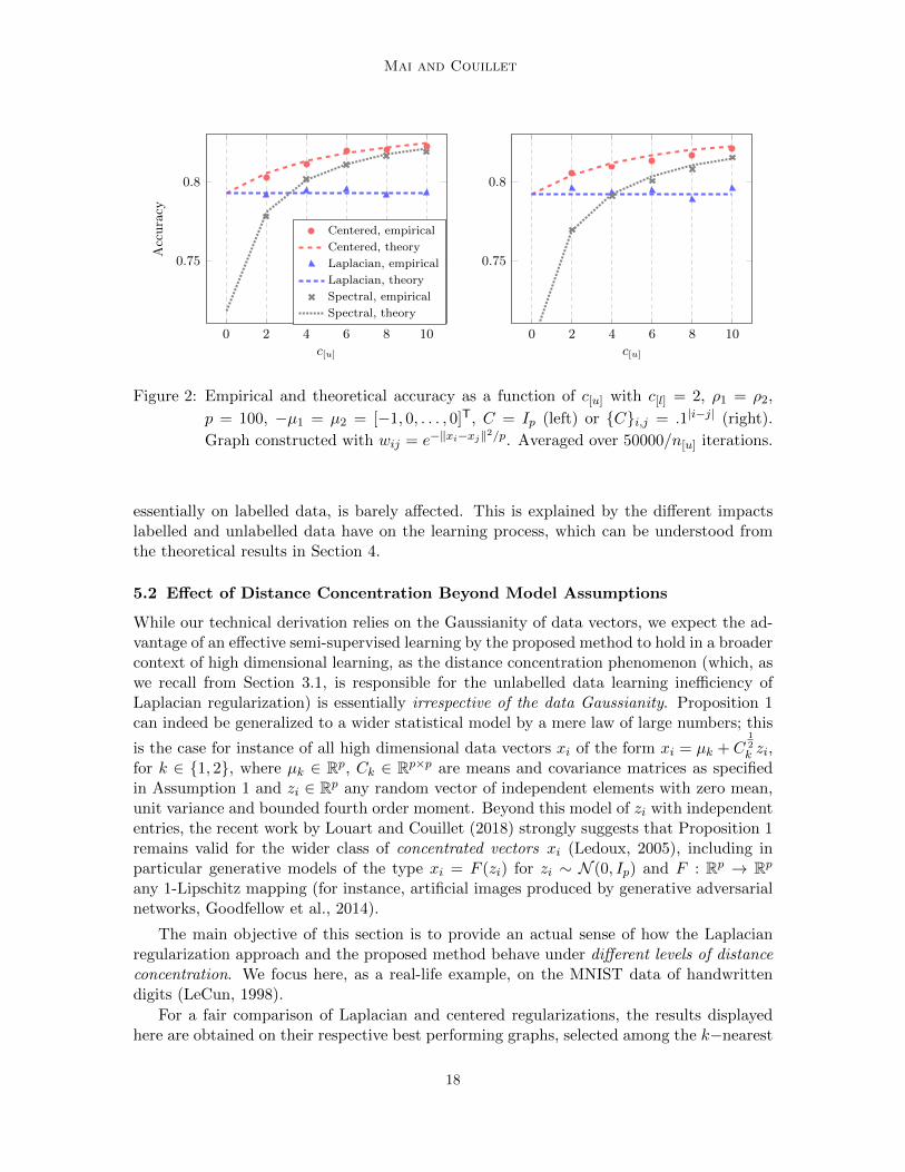
Under a non-trivial Gaussian mixture model setting (see caption) with p = 100, Figure 2demonstrates a sharp prediction of the average empirical performance by the asymptoticanalysis. As revealed by the theoretical results, the Laplacian regularization method failsto learn effectively from unlabelled data, causing it to be outperformed by the purely unsu-pervised spectral clustering approach (for which the labelled data are treated as unlabelledones) for sufficiently numerous unlabelled data. The performance curve of the proposedcentered regularization algorithm, on the other hand, is consistently above that of spec-tral clustering, with a growing advantage over Laplacian regularization as the number ofunlabelled data increases.
Figure 2 also interestingly shows that the unsupervised performance of spectral clus-tering is noticeably reduced when the covariance matrix of the data distribution changesfrom the identity matrix to a slightly disrupted model (here for {C}i,j = .1|i−j|). On thecontrary, the Laplacian regularization, the high dimensional performance of which relies
17
Mai and Couillet
0 2 4 6 8 10
0.75
0.8
c[u]
Acc
ura
cy
Centered, empirical
Centered, theory
Laplacian, empirical
Laplacian, theory
Spectral, empirical
Spectral, theory
0 2 4 6 8 10
0.75
0.8
c[u]
Figure 2: Empirical and theoretical accuracy as a function of c[u] with c[l] = 2, ρ1 = ρ2,
p = 100, −µ1 = µ2 = [−1, 0, . . . , 0]T, C = Ip (left) or {C}i,j = .1|i−j| (right).
Graph constructed with wij = e−‖xi−xj‖2/p. Averaged over 50000/n[u] iterations.
essentially on labelled data, is barely affected. This is explained by the different impactslabelled and unlabelled data have on the learning process, which can be understood fromthe theoretical results in Section 4.
5.2 Effect of Distance Concentration Beyond Model Assumptions
While our technical derivation relies on the Gaussianity of data vectors, we expect the ad-vantage of an effective semi-supervised learning by the proposed method to hold in a broadercontext of high dimensional learning, as the distance concentration phenomenon (which, aswe recall from Section 3.1, is responsible for the unlabelled data learning inefficiency ofLaplacian regularization) is essentially irrespective of the data Gaussianity. Proposition 1can indeed be generalized to a wider statistical model by a mere law of large numbers; this
is the case for instance of all high dimensional data vectors xi of the form xi = µk + C12k zi,
for k ∈ {1, 2}, where µk ∈ Rp, Ck ∈ Rp×p are means and covariance matrices as specifiedin Assumption 1 and zi ∈ Rp any random vector of independent elements with zero mean,unit variance and bounded fourth order moment. Beyond this model of zi with independententries, the recent work by Louart and Couillet (2018) strongly suggests that Proposition 1remains valid for the wider class of concentrated vectors xi (Ledoux, 2005), including inparticular generative models of the type xi = F (zi) for zi ∼ N (0, Ip) and F : Rp → Rpany 1-Lipschitz mapping (for instance, artificial images produced by generative adversarialnetworks, Goodfellow et al., 2014).
The main objective of this section is to provide an actual sense of how the Laplacianregularization approach and the proposed method behave under different levels of distanceconcentration. We focus here, as a real-life example, on the MNIST data of handwrittendigits (LeCun, 1998).
For a fair comparison of Laplacian and centered regularizations, the results displayedhere are obtained on their respective best performing graphs, selected among the k−nearest
18
Consistent Semi-Supervised Graph Regularization for High Dimensional Data
Digits (3, 5) Digits (7, 8, 9)
0 0.5 1 1.5 2
0
0.1
Normalized pairwise distances
Rel
ati
ve
freq
uen
cyIntra-class
Inter-class
0 0.5 1 1.5 2
0
0.1
Normalized pairwise distances
100 300 5000.82
0.84
0.86
0.88
0.9
n[u]
Acc
ura
cy
Lapalcian regularization
Centered regularization
200 400 600
0.8
0.82
0.84
0.86
0.88
n[u]
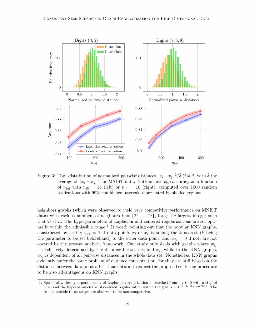
Figure 3: Top: distribution of normalized pairwise distances ‖xi−xj‖2/δ (i 6= j) with δ theaverage of ‖xi − xj‖2 for MNIST data. Bottom: average accuracy as a functionof n[u] with n[l] = 15 (left) or n[l] = 10 (right), computed over 1000 randomrealizations with 99% confidence intervals represented by shaded regions.
neighbors graphs (which were observed to yield very competitive performance on MNISTdata) with various numbers of neighbors k = {21, . . . , 2q}, for q the largest integer suchthat 2q < n. The hyperparameters of Laplacian and centered regularizations are set opti-mally within the admissible range.1 It worth pointing out that the popular KNN graphs,constructed by letting wij = 1 if data points xi or xj is among the k nearest (k beingthe parameter to be set beforehand) to the other data point, and wij = 0 if not, are notcovered by the present analytic framework. Our study only deals with graphs where wijis exclusively determined by the distance between xi and xj , while in the KNN graphs,wij is dependent of all pairwise distances in the whole data set. Nonetheless, KNN graphsevidently suffer the same problem of distance concentration, for they are still based on thedistances between data points. It is thus natural to expect the proposed centering procedureto be also advantageous on KNN graphs.
1. Specifically, the hyperparameter a of Laplacian regularization is searched from −2 to 0 with a step of0.02, and the hyperparameter α of centered regularization within the grid α = 10{−3,−2.9,...,2.9,3}. Theresults outside these ranges are observed to be non-competitive.
19
Mai and Couillet
SNR = −5dB SNR = −10dB
0.6 0.8 1 1.2 1.4
0
0.1
Normalized pairwise distances
Rel
ati
ve
freq
uen
cyIntra-class
Inter-class
0.6 0.8 1 1.2 1.4
0
0.1
Normalized pairwise distances
200 400 600
0.68
0.7
0.72
0.74
n[u]
Acc
ura
cy
Lapalcian regularization
Centered regularization
200 400 600 800
0.5
0.55
0.6
0.65
n[u]
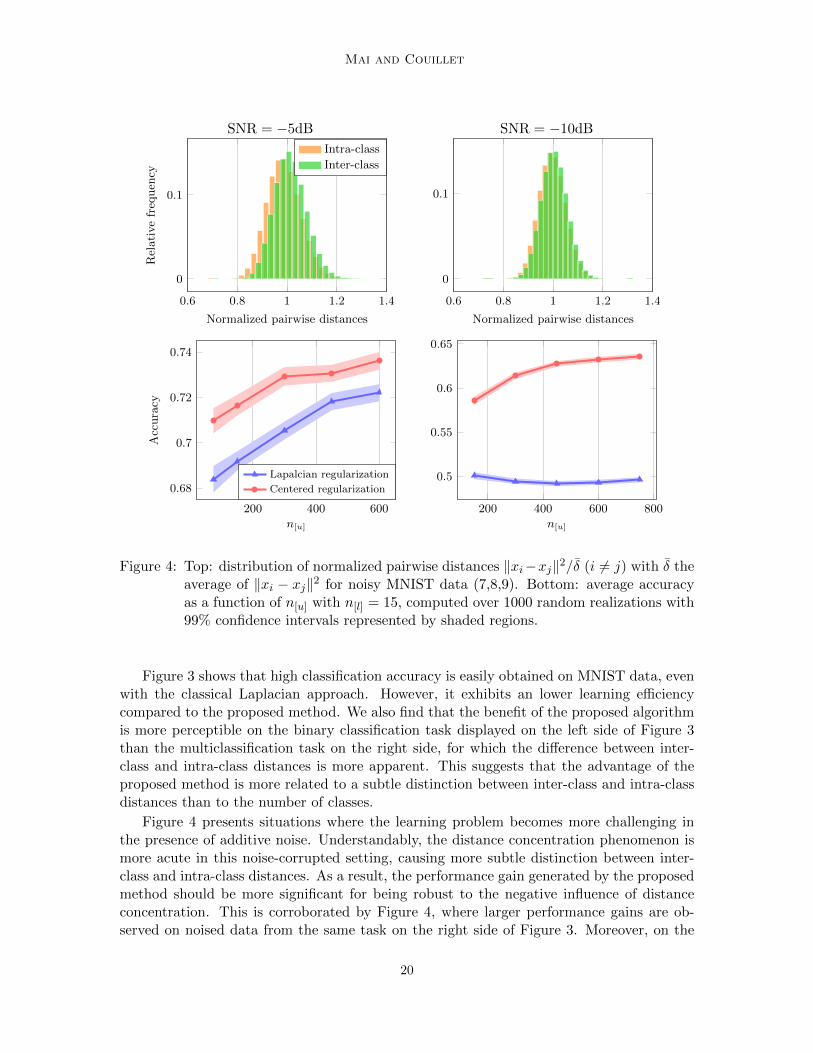
Figure 4: Top: distribution of normalized pairwise distances ‖xi−xj‖2/δ (i 6= j) with δ theaverage of ‖xi − xj‖2 for noisy MNIST data (7,8,9). Bottom: average accuracyas a function of n[u] with n[l] = 15, computed over 1000 random realizations with99% confidence intervals represented by shaded regions.
Figure 3 shows that high classification accuracy is easily obtained on MNIST data, evenwith the classical Laplacian approach. However, it exhibits an lower learning efficiencycompared to the proposed method. We also find that the benefit of the proposed algorithmis more perceptible on the binary classification task displayed on the left side of Figure 3than the multiclassification task on the right side, for which the difference between inter-class and intra-class distances is more apparent. This suggests that the advantage of theproposed method is more related to a subtle distinction between inter-class and intra-classdistances than to the number of classes.
Figure 4 presents situations where the learning problem becomes more challenging inthe presence of additive noise. Understandably, the distance concentration phenomenon ismore acute in this noise-corrupted setting, causing more subtle distinction between inter-class and intra-class distances. As a result, the performance gain generated by the proposedmethod should be more significant for being robust to the negative influence of distanceconcentration. This is corroborated by Figure 4, where larger performance gains are ob-served on noised data from the same task on the right side of Figure 3. Moreover, on the
20
Consistent Semi-Supervised Graph Regularization for High Dimensional Data
right display of Figure 4, where the similarity information is seriously disrupted by the ad-ditive noise, we observe the anticipated saturation effect when increasing n[u] for Laplacianregularization, in contrast to the growing performance of the proposed approach. This sug-gests, in conclusion, that regularization with centered similarities has a competitive, if notsuperior, performance in various situations, and yields particularly significant performancegains when the distinction between intra-class and inter-class similarities is quite subtle.
6. Further Discussion and Support
We start this section by presenting other graph-based semi-supervised learning methods anddiscussing them in relation to the regularization approaches investigated in this article. Toevaluate the ability of these SSL methods to optimally exploit the information in partiallylabelled data sets, we use the recent results of Lelarge and Miolane (2019) as a referencepoint, where the best achievable semi-supervised learning performance on high dimensionalGaussian mixture data with identity covariance matrices was characterized. For a broaderdiscussion on the applicability of the centering approach, we propose in Section 6.3.1 ahigher-order version of centered regularization adapted from the iterated Laplacian method(Zhou and Belkin, 2011), which serves as an example for applying centered similarities be-yond the standard Laplacian regularization. Our experiments in Section 6.3.2 demonstratethe practical interest of centered similarities on various benchmark data sets, and show inparticular that the algorithm combining centered simliarities with the iterated techniqueof higher-order regularization helps substantially increase the competitiveness of graph reg-ularization as an SSL approach on challenging data sets. We conclude by remarking inSection 6.4 that the sparsity of the weight matrix can also be exploited for improving thecomputational efficiency of centered regularization with the help of Woodbury’s inversionformula.
6.1 Related Methods
We review first some competitive variants of Laplacian regularization before presentinganother major approach of graph-based semi-supervised learning which relies explicitly onthe spectral decomposition of Laplacian matrices.
6.1.1 Variants of Laplacian Regularization
The method of Laplacian regularization has been found by Nadler et al. (2009) to sufferfrom the “score flatness” problem where unlabelled data scores fi concentrate around thesame value (i.e., fi = c+ o(1) for some constant c) when the number of unlabelled samplesis exceedingly large compared to that of labelled ones (i.e., n[u]/n[l] → ∞). Following thisdiscovery, several regularization techniques have been proposed to adapt the original methodto ensure well-behaved scores, which will be presented in this section. On a related note,the analysis of Mai and Couillet (2018) (which motivated the present study) pointed outthat, in high dimensions, the phenomenon of flat unlabelled data scores occurs even whenthe number of unlabelled samples is comparable to that of labelled ones. As can be easilydeduced from our study, the problem of flat unlabelled scores is addressed by the centeredregularization method in the more challenging setting of high dimensional learning.
21
Mai and Couillet
Higher Order Regularization. A well-studied approach to address the problem of flatunlabelled scores revealed by Nadler et al. (2009) is higher-order regularization. There existmainly two types of higher-order regularization: iterated Laplacian and `p-based Laplacian.The method of iterated Laplacian regularization consists in using the powers of Laplacianmatrices for constructing high-order regularizers fTLqf of graph smoothness. It was shownby Zhou and Belkin (2011) to yield non-flat unlabelled scores. The `p-based Laplacian regu-larization achieves this by forcing a stronger constrain
∑ni,j=1wij |fi−fj |q on the smoothness
(Zhou and Scholkopf, 2005; El Alaoui et al., 2016). Another method in the same vein isgame-theoretic p-Laplacian (Rios et al., 2019), which does not arise through an optimiza-tion problem and tends to be numerically better conditioned. In comparison, the iteratedapproach is more computationally efficient as it assumes an explicit solution, whereas themethod of `p-based Laplacian regularization calls for practical algorithms to solve more ef-ficiently the implicit optimization (Rios et al., 2019). Also, the iterated Laplacian is foundto outperform p-voltages Laplacian regularization (Bridle and Zhu, 2013), a dual version of`p-based Laplacian in the context of electrical networks. In addition to avoiding the score‘flatness’ issue, high-order regularizers fTLqf and their extensions fTg(L)f (Smola andKondor, 2003) obviously benefit from more degrees of freedom to improve the classificationperformance.
Weighted Nonlocal Laplacian. Other than the methods of high-order regularization,the approach of weighted nonlocal Laplacian (Shi et al., 2017) has also been observed to beeffective in combating the score flatness problem. By changing the optimization to
minf[u]∈R
n[u]
n∑i=n[l]+1
n∑j=n[l]+1
wij(fi − fj)2 +n
n[l]
n[l]∑j=1
wij(fi − fj)2 ,
it places a higher weight of n/n[l] on the smoothness penalty between unlabelled data scoresand fixed non-flat ones on labelled points.
6.1.2 Eigenvector-Based Methods
Aside from graph regularization methods, another popular graph-based semi-supervisedapproach exists which takes advantage of the spectral information of Laplacian matrices(Belkin and Niyogi, 2003). Rather than regularizing f over the graph, this method computesfirst the eigenmap of Laplacian matrices, then uses a certain number s of eigenvectorsE = [e1, . . . , es] associated with the smallest eigenvalues to build a linear subspace andsearch within this space for an f which minimizes ‖f[l] − y[l]‖. By the method of least
squares, f = Ea with a = (ET[l]E[l])
−1ET[l]y[l].
As an advantage of using the spectral information, this eigenvector-based method isguaranteed to achieve at least the performance of spectral clustering, as opposed to theLaplacian regularization approach. On the other hand, the regularization approach doesnot have a performance which depends crucially on how well the class signal is captured by asmall number of eigenvectors, as it uses the graph matrix as a whole. Another benefit of thegraph regularization approach is that it can be easily incorporated into other algorithmsas an additional term in the loss function (e.g., Laplacian SVMs). With our proposedalgorithm of centered regularization, a consistent learning of unlabelled data, related to
22
Consistent Semi-Supervised Graph Regularization for High Dimensional Data
the performance of spectral clustering, can also be achieved by the graph regularizationapproach. Moreover, the proposed method has a theoretically-proven efficient usage oflabelled data which is absent in the eigenvector-based method.
6.2 Optimal Performance on Isotropic Gaussian Data of High Dimensionality
A very recent work of Lelarge and Miolane (2019) has established the optimal performanceof semi-supervised learning on a high dimensional Gaussian mixture data model N (±µ, Ip),with identity covariance matrices.2 In this work, a method of Bayesian estimation is identi-fied as the one achieving the optimal performance. However, as pointed out by the authors,this method is computationally expensive except on fully labelled data sets and approxi-mations are needed for practical usage.
By comparing the results of Lelarge and Miolane (2019) with our performance analysisin Section 4, we find that the method of centered regularization achieves an optimal per-formance on fully labelled data sets and a nearly optimal one on partially labelled sets.3
Numerical results are given in Figure 5, where the classification accuracy of the centeredregularization method, computed from Theorem 3 and maximized over the hyperparametere, is observed to be extremely close to the optimal performance provided by Lelarge and Mi-olane (2019). Hence, the centered regularization method can be used as a computationallyefficient alternative to the Bayesian approach which yields the best achievable performance.In contrast, other graph-based semi-supervised learning algorithms are much less effectivein reaching the optimal performance, as can be observed from Figure 6.
We remark also that the iterated Laplacian regularization method appears to be lessefficient in exploiting unlabelled data and so is the eigenvector-based method in learningfrom labelled data. As can be observed in Figure 6, the iterated Laplacian regularizationmethod falls notably short of approaching the optimal performance when the value of myielding the highest accuracy is further away from 1 (scenarios depicted by the blue curvesin the figure). Since we retrieve the standard Laplacian regularization at m = 1, which givesthe optimal performance in the absence of unlabelled data, the performance gain yielded bythe iterated Laplacian regularization technique over the Laplacian method is mainly broughtby the utilization of unlabelled data at higher m. However, as demonstrated in Figure 6, theutilization of unlabelled data at higher m is unsatisfactory in allowing the method to reachthe optimal semi-supervised learning performance. Since the eigenvector-based approach isreduced to the purely unsupervised method of spectral clustering at s = 1, the same remarkcan be made with respect to its labelled data learning efficiency.
6.3 Applicability of Centered Similarities and High-Order Regularization
The focus of this article is to promote the usage of centered similarities in graph regular-ization for semi-supervised learning. This fundamental idea can also be applied togetherwith other regularization techniques. In this section, we start by presenting a higher-orderversion of centered regularization that borrows from iterated Laplacian. To investigate thepractical potential of centered similarities, we test the proposed method of centered regu-
2. To the authors’ knowledge, more general results (e.g., with arbitrary covariance matrices) are currentlyout-of-reach.
3. We refer to Appendix D for some theoretical details.
23

Mai and Couillet
2 4 6 8 10
0.75
0.8
0.85
0.9
c[u]
Acc
ura
cy
Baysian (optimal)
Centered regularization
Figure 5: Asymptotic accuracy on isotropic Gaussian mixture data. Performance curves asa function of c[u] with c[l] = 1/2, for (from top to bottom) ‖µ‖2 = 2, 4/3, or 1.
Centered Iterated Eigenvector-based
−2 0 20.74
0.76
0.78
0.8
0.82
Acc
ura
cy
c[l] = 1
c[l] = 3
0 100 200 0 100 200
−2 0 2
0.66
0.68
0.7
0.72
Acc
ura
cy
0 100 200 0 100 200
log10 α m s
Figure 6: Empirical accuracy of graph-based SSL algorithms at different values of hyperpa-rameters for isotropic Gaussian mixture data with p = 60, n = 360 and ‖µ‖2 = 1(bottom) or ‖µ‖2 = 2 (top). Averaged over 1000 realizations. Best empiricalvalue marked in circle and the asymptotic optimum in cross.
24

Consistent Semi-Supervised Graph Regularization for High Dimensional Data
larization and its higher-order variant on several benchmark data sets. Our experimentssupport the benefit of centered similarities, especially on challenging data sets. We find im-portantly that the proposed higher-order centered regularization, which combines the ideasof centered similarities and iterated regularization, yields a very competitive performancewhen compared to not only related graph-based methods but also a wide range of popularSSL approaches.
6.3.1 Higher-Order Centered Regularization
It is easy to check that all exponents of a centered simliarity matrix W enjoy the same prop-erty of being orthogonal to the constant vector 1n. It is thus possible to apply polynomialfunctions of W in the search of a better centered regularizer. Finding the right parametriza-tion for the polynomial function can be challenging. Comparing (2) and (9), we notice thatthe matrix L = λIn − W plays the same role in centered regularization as the Laplacianmatrix L in Laplacian regularization. We then borrow the idea from iterated Laplacian topropose a higher-order centered regularization method, which consists in simply replacingL = λIn − W in (9) with its exponents L(q) = (λIn − W )q, leading to
f[u] = −L(q)−1[uu] L
(q)[ul]f[l] (17)
The method of iterated centered regularization is formalized in Algorithm 2.
Algorithm 2 Graph-Based Iterated Centered Regularization
1: Input: n[l] pairs of labelled points and labels {(xi, yi)}n[l]
i=1, n[u] unlabelled data{xi}ni=n[l]+1
, parameters α ∈ R+, q ∈ N+.
2: Output: Classification score vector of unlabelled data f[u] ∈ Rn[u]
3: Define the similarity matrix W = {wi,j}ni,j=1 with wij reflecting the closeness betweenxi and xj .
4: Compute the centered similarity matrix W by (7) and the balanced labels f[l] by (4).
5: Set λ = (α+ 1)‖W‖, L(q) = (λIn − W )q, and compute f[u] by (17).
6.3.2 Experimental Results and Comparison to Other Methods
To investigate the practical potential of centered similarities, we test in this section the pro-posed methods of standard and higher-order centered regularization on several benchmarkdata. We first focus on the comparison with the related graph-based SSL methods presentedin Section 6.1, before moving on to a wider range of competitors. Our results attest to thegeneral interest of centered similarities for improving over the classical Laplacian approach.Remarkably, the algorithm of iterated centered regularization, which inherits the strengthsof both iterated and centered approaches, is identified as a powerful competitor not onlyagainst other graph-based algorithms but also against a wide range of SSL methods sur-veyed by Chapelle et al. (2010), with an advantage which tends to be more observable onchallenging data sets.
Firstly, to compare graph-based SSL methods, we conduct experiments on the MINSTdata of handwritten digits and the RCV1 data of categorized newswire stories. For MNIST
25

Mai and Couillet
n N/6 N/2 N
MNIST
Laplacian 53.9± 11.2 44.7± 10.6 33.5± 14.0Centered 81.4± 2.6 85.3± 2.5 86.3± 3.9
Iterated Laplacian 81.7± 3.5 83.7± 3.6 86.4± 5.5Iterated Centered 83.2± 2.7 86.8± 3.7 88.4± 3.2`p-based Laplacian 72.7± 3.5 75.9± 4.0 76.0± 2.7
WN Laplacian 78.0± 3.2 79.0± 4.3 79.1± 4.1Eigenvector-based 79.9± 3.7 85.4± 4.2 86.6± 3.8
RCV1
Laplacian 36.8± 12.9 34.2± 9.7 33.4± 9.6Centered 78.7± 2.7 79.0± 3.2 79.1± 2.3
Iterated Laplacian 81.0± 2.1 81.4± 3.2 80.8± 5.6Iterated Centered 83.8± 2.4 84.5± 2.1 84.8± 2.7
WN Laplacian 70.1± 3.4 71.7± 4.9 71.8± 4.8Eigenvector-based 81.8± 5.4 82.1± 4.5 82.8± 3.0
Table 1: Classification accuracy (%) of graph-based SSL algorithms averaged over 10 ran-dom splits, for n[l] = 5K with K the number of classes (K = 10 for MNIST, K = 4for RCV1) and n = {N/6, N/2, N} with N the total sample number (N = 60000for MNIST, N = 19000 for RCV1).
data, we use, as in the experiments of Section 5.2, the raw version4 of vectorized pixels(LeCun, 1998), and for RCV1 data, we retrieve from the paper of Cai and He (2011) apreprocessed four-class version5 of tf-idf feature vectors. As suggested in the previous studies(Belkin and Niyogi, 2003; Zhou and Belkin, 2011; Johnson and Zhang, 2007), satisfyingperformance can be observed on MNIST data for KNN graphs with k ∼ 10 and on RCV1data for k ∼ 100; we will test with k over 10 × 2{0,1,...,6}. To judge the potential of graph-based methods, we report the best model performance for each method. We test the threecommon versions of Laplacian matrices L,Ls, Lr presented in Section 2.1 for Laplacianmethods. The hyperparameter q of higher-order regularization algorithms is tried on 2{1,2,3},the hyperparameter s of the eigenvector-based method is searched among all possible values(i.e., all integers from 1 to n[l]), and the hyperparameter α of centered regularization takes
its values in 10{−3,−2,−1,0}. The results are displayed in Table 16, where the advantage ofcentered similarities is supported by performance gains over the Laplacian methods. Wealso find that the iterated technique is powerful for improving the performance of centeringregularization, which alone can be insufficient for producing superior results.
To evaluate the competitiveness of centered regularization beyond the family of graph-based methods, we report its performance on SSL benchmark data sets7 established by
4. Available for download at http://yann.lecun.com/exdb/mnist/ .5. Available for download at http://www.cad.zju.edu.cn/home/dengcai/Data/TextData.html .6. The performance of the `p-based Laplacian is not reported on RCV1 data due to the unsatisfying
performance at small k and the very slow computation at large k.7. Available for download at http://olivier.chapelle.cc/ssl-book/benchmarks.html .
26
Consistent Semi-Supervised Graph Regularization for High Dimensional Data
g241c g241d Digit1 USPS BCI Text
Laplacian+CMN(Chapelle et al., 2010)
77.95 71.80 96.85 93.64 53.78 74.29
Best over 13 Algo(Chapelle et al., 2010)
86.51 95.05 97.56 95.32 68.64 76.91
Iterated Laplacian(Zhou and Belkin, 2011)
85.18 89.45 97.78 96.04 56.22 74.23
Iterated Centered 87.18 86.31 97.50 94.40 70.78 76.96
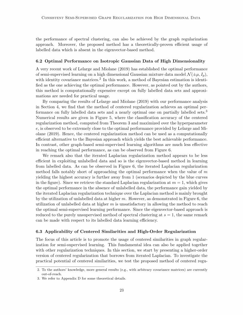
Table 2: Classification accuracy (%) on SSL benchmarks with n[l] = 100 and n = 1500,averaged over 12 random splits.
Chapelle et al. (2010) and tested for an extensive variety of SSL methods including Lapla-cian regularization (with a class mass normalization technique (CMN) for performanceimprovement). The same trials were also carried out by Zhou and Belkin (2011) for themethod of iterated Laplacian regularization.
To produce our results, we simply use a KNN graph with k = 10 on the “Digit1” and“USPS”8 tasks of image data; for the rest, we switch to fully connected graphs wij =exp(−‖xi − xj‖2/2σ2) as in the experiments of Chapelle et al. (2010); Zhou and Belkin(2011). Also following the settings for the Laplacian and iterated Laplacian methods, thehyperparameters are determined by a (10-fold) cross-validation on the first split of eachdata set, searched over the grid σ = {d/3, 3d} for d the average pairwise distance, q ={21, 24, 27, 210}, and with α set to 10−3. Our results are reported in Table 2, along withthe performances of the iterated Laplacian and Laplacian regularization methods obtainedby Chapelle et al. (2010); Zhou and Belkin (2011), as well as the best performance over 13algorithms tested by Chapelle et al. (2010).
As can be observed in Table 2, the combined approach of iterated and centering tech-niques has a remarkable competitiveness overall. We note in particular its superiority onthe three most difficult tasks “g241c”, “BCI” and “Text” with lowest best accuracy, wherethe iterated technique alone fails to approach the best performance over 13 algorithms. Thetask on which the proposed method yields comparably worst results is “g241d”, observedto be quite unstable with huge gaps between the best performing algorithm and the rest(Chapelle et al., 2010).
6.4 Computational Cost on Sparse Graphs
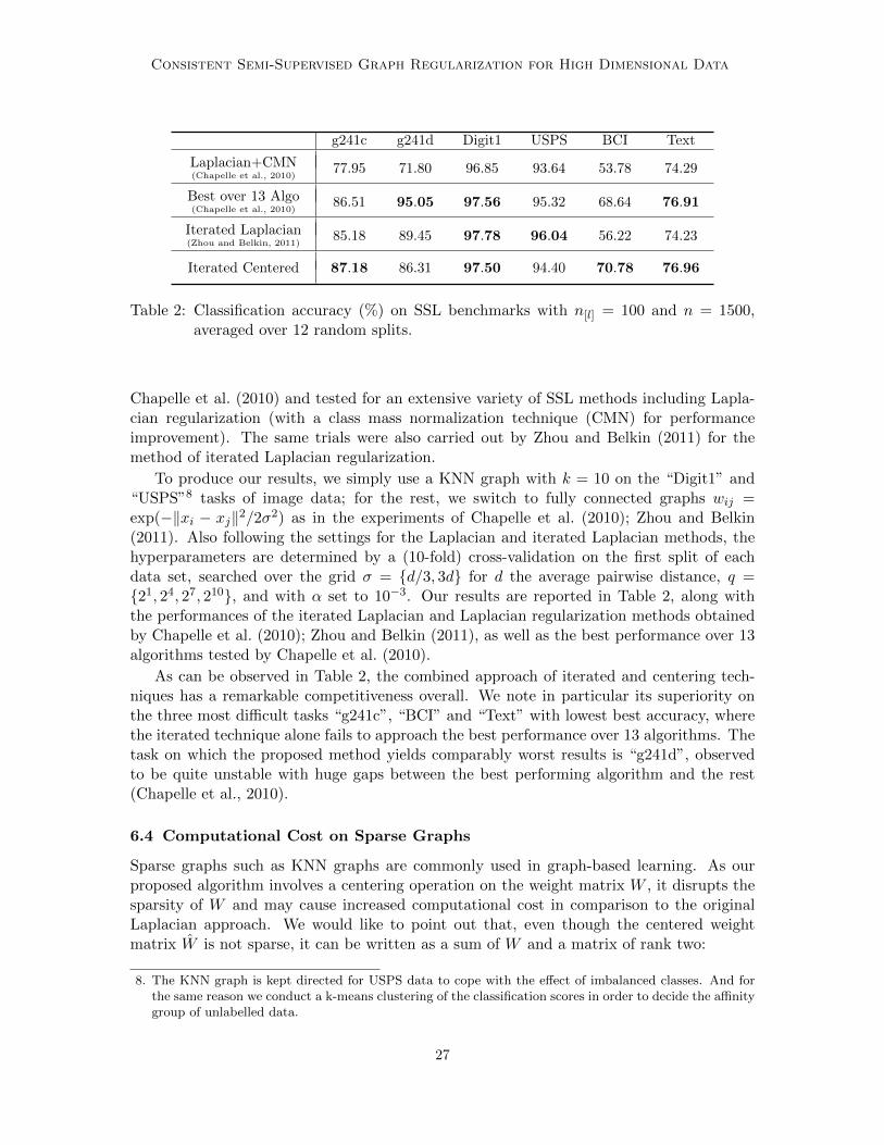
Sparse graphs such as KNN graphs are commonly used in graph-based learning. As ourproposed algorithm involves a centering operation on the weight matrix W , it disrupts thesparsity of W and may cause increased computational cost in comparison to the originalLaplacian approach. We would like to point out that, even though the centered weightmatrix W is not sparse, it can be written as a sum of W and a matrix of rank two:
8. The KNN graph is kept directed for USPS data to cope with the effect of imbalanced classes. And forthe same reason we conduct a k-means clustering of the classification scores in order to decide the affinitygroup of unlabelled data.
27
Mai and Couillet
W = W +[1n v
]A
[1TnvT
]
where v = W1n and A =
[(1TnW1n)/n2 −1/n−1/n 0
]. Using Woodbury’s inversion formula, we
can then decompose the inverse of λIn[u]−W[uu] as the inverse of λIn[u]
−W[uu] plus a matrixof rank two as:
(λIn[u]
− W[uu]
)−1= Q−Q
[1n[u]
v[u]](
A−1 +
[1Tn[u]
vT[u]
]Q[1n[u]
v[u]])−1 [1Tn[u]
vT[u]
]Q
where Q = (λIn[u]− W[uu])
−1. Therefore, the complexity of computing the solution ofcentered regularization can be reduced to that of computing QW[ul]f[l], which benefits fromthe sparsity of W . Similar reasoning can also be made for the iterated regularizationalgorithm presented in section 6.3.1.
7. Concluding Remarks
The key to the proposed semi-supervised learning method lies in the replacement of con-ventional Laplacian regularizers by a new graph smoothness regularizer with centered simi-larities. The motivation is rooted in the failure of the Laplacian regularization approach tolearn effectively from unlabelled data due to the concentration of pairwise distances betweenhigh dimensional data vectors. As anticipated by our theoretical results, the proposed cen-tered regularization method produced large performance gains over the standard Laplacianregularization method when the aforementioned distance concentration problem is severe,thanks to an effective learning from both labelled and unlabelled data learning. Moreover, itwas observed that the proposed algorithm can further improve the performance even on datasets with weak distance concentration, for which the standard Laplacian approach exhibitsa clear performance growth with respect to unlabelled data. Other than improving uponthe Laplacian regularization method, the proposed algorithm is also theoretically proven toenjoy a near-optimal performance of semi-supervised learning on isotropic Gaussian mixturedata. From a general perspective, the extended advantage of centered regularization beyondthe initial motivation suggests that placing oneself under the challenging setting of high di-mensional learning can help identify and address some underlying issues compromising theperformance of popular learning heuristics.
As the usage of centered similarities constitutes a fundamental update to the classi-cal Laplacian regularization approach, it would be interesting to investigate whether otheralgorithms involving Laplacian regularizers benefit from the same update. In this articlewe proposed additionally a higher-order version of centered regularization based on theiterated Laplacian method (Zhou and Belkin, 2011). The empirical analysis on variousreal-world data sets showed that adopting centered similarities can improve substantiallythe performance on difficult tasks where the Laplacian methods are observed to underper-form. Future studies can be devoted to analysing and adapting more involved methods likeLaplacian support vector machines (Belkin et al., 2006), which combines the optimization
28
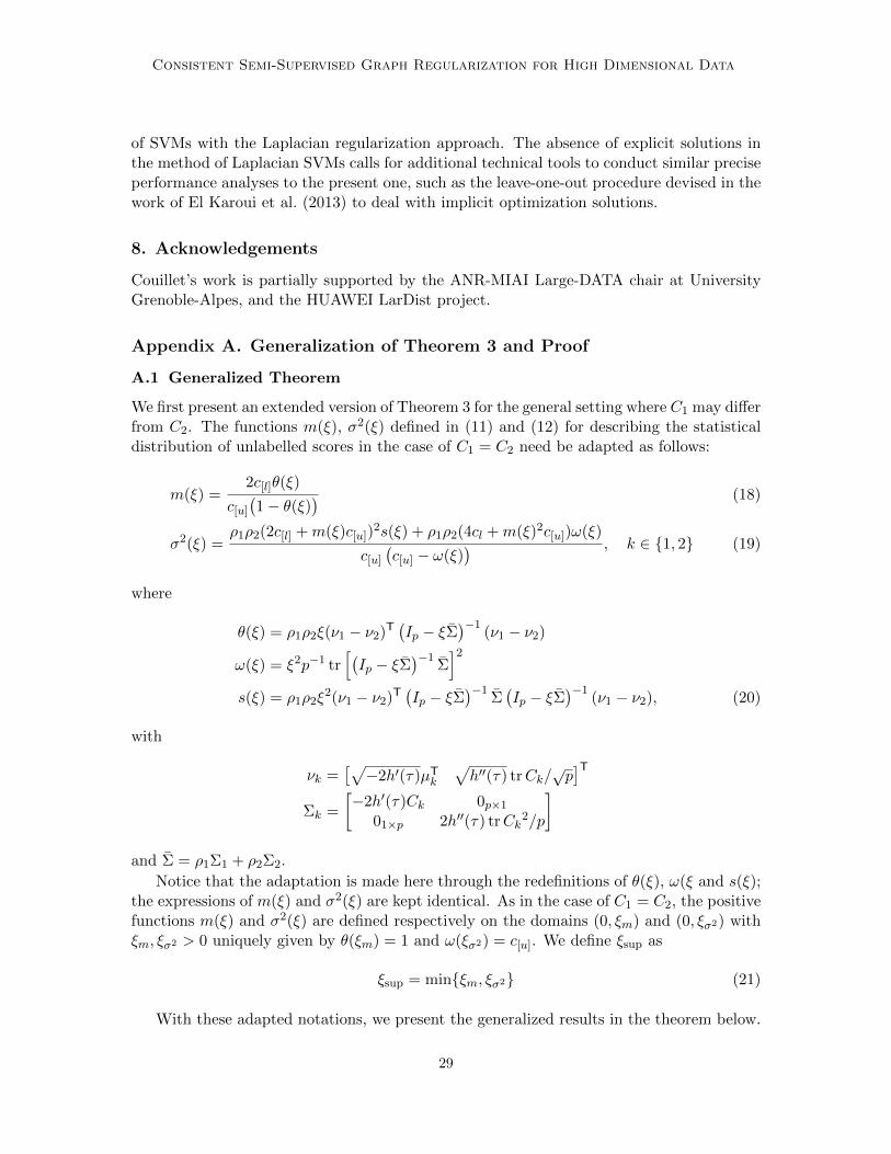
Consistent Semi-Supervised Graph Regularization for High Dimensional Data
of SVMs with the Laplacian regularization approach. The absence of explicit solutions inthe method of Laplacian SVMs calls for additional technical tools to conduct similar preciseperformance analyses to the present one, such as the leave-one-out procedure devised in thework of El Karoui et al. (2013) to deal with implicit optimization solutions.
8. Acknowledgements
Couillet’s work is partially supported by the ANR-MIAI Large-DATA chair at UniversityGrenoble-Alpes, and the HUAWEI LarDist project.
Appendix A. Generalization of Theorem 3 and Proof
A.1 Generalized Theorem
We first present an extended version of Theorem 3 for the general setting where C1 may differfrom C2. The functions m(ξ), σ2(ξ) defined in (11) and (12) for describing the statisticaldistribution of unlabelled scores in the case of C1 = C2 need be adapted as follows:
m(ξ) =2c[l]θ(ξ)
c[u](1− θ(ξ)
) (18)
σ2(ξ) =ρ1ρ2(2c[l] +m(ξ)c[u])
2s(ξ) + ρ1ρ2(4cl +m(ξ)2c[u])ω(ξ)
c[u](c[u] − ω(ξ)
) , k ∈ {1, 2} (19)
where
θ(ξ) = ρ1ρ2ξ(ν1 − ν2)T(Ip − ξΣ
)−1(ν1 − ν2)
ω(ξ) = ξ2p−1 tr[(Ip − ξΣ
)−1Σ]2
s(ξ) = ρ1ρ2ξ2(ν1 − ν2)T
(Ip − ξΣ
)−1Σ(Ip − ξΣ
)−1(ν1 − ν2), (20)
with
νk =[√−2h′(τ)µTk
√h′′(τ) trCk/
√p]T
Σk =
[−2h′(τ)Ck 0p×1
01×p 2h′′(τ) trCk2/p
]and Σ = ρ1Σ1 + ρ2Σ2.
Notice that the adaptation is made here through the redefinitions of θ(ξ), ω(ξ and s(ξ);the expressions of m(ξ) and σ2(ξ) are kept identical. As in the case of C1 = C2, the positivefunctions m(ξ) and σ2(ξ) are defined respectively on the domains (0, ξm) and (0, ξσ2) withξm, ξσ2 > 0 uniquely given by θ(ξm) = 1 and ω(ξσ2) = c[u]. We define ξsup as
ξsup = min{ξm, ξσ2} (21)
With these adapted notations, we present the generalized results in the theorem below.
29
Mai and Couillet
Theorem 8 Let Assumption 1 hold, the function h of (1) be three-times continuously dif-ferentiable in a neighborhood of τ , f[u] be the solution of (8) with fixed norm n[u]e
2, andwith the notations of m(ξ), σ2(ξ), ξsup given in (18), (19), (21). Then, for n[l] + 1 ≤ i ≤ n(i.e., xi unlabelled) and xi ∈ Ck,
fiL→ N
((−1)k(1− ρk)m, σ2k
)where
m = m(ξe)
σ2k = c−2[u] ρ1ρ2[(2c[l] +m(ξe)c[u])
2sk(ξe) + (4cl +m(ξe)2c[u] + σ2(ξe)c[u])ω(ξe)
]with
sa(ξe) = ρ1ρ2ξ2e (ν1 − ν2)T
(Ip − ξeΣ
)−1Σk
(Ip − ξeΣ
)−1(ν1 − ν2), a ∈ {1, 2},
and ξe ∈ (0, ξsup) uniquely given by
ρ1ρ2m(ξe)2 + σ2(ξe) = e2.
A.2 Proof of Generalized Theorem
The proof of Theorem 8 relies on a leave-one-out approach, in the spirit of El Karoui et al.(2013), along with arguments from previous related analyses (Couillet and Benaych-Georges,2016; Mai and Couillet, 2018) based on random matrix theory .
A.2.1 Main Idea
The main idea of the proof is to first demonstrate that for unlabelled data scores fi (i.e.,with i > n[l]),
fi = γβ(i)Tφc(xi) + oP (1) (22)
where γ is a finite constant, φc a certain mapping from the data space that we shall define,and β(i) a random vector independent of φc(xi). Additionally, we shall show that
β(i) =1
p
n∑j=1
fjφc(xj) + ε (23)
with ‖ε‖/‖β(i)‖ = oP (1).
As a consequence of (22), the statistical behavior of the unlabelled data scores canbe understood through that of β(i), which itself depends on the unlabelled data scores asdescribed by (23). By combining (22) and (23), we thus establish the equations ruling theasymptotic statistical behavior (i.e., mean and variance) of the unlabelled data scores fi.
30

Consistent Semi-Supervised Graph Regularization for High Dimensional Data
A.2.2 Detailed Arguments
In addition to the notations given in the end of the introduction (Section 1), we specifythat when multidimensional objects are concerned, O(un) is understood entry-wise. Thenotation O‖·‖ is understood as follows: for a vector v, v = O‖·‖(un) means its Euclideannorm is O(un) and for a square matrix M , M = O‖·‖(un) means that the operator norm ofM is O(un).
First note that, as wij = h(‖xi−xj‖2/p) = h(τ)+O(p−12 ), Taylor-expanding wij around
h(τ) gives (see Appendix C for a detailed proof) W = O‖·‖(1) and
W =1
pΦTΦ + [h(0)− h(τ) + τh′(τ)]Pn +O‖·‖(p
− 12 ) (24)
where Pn = In − 1n1n1Tn , and Φ = [φ(x1), . . . , φ(xn)] = [φ(x1), . . . , φ(xn)]Pn with
φ(xi) =[√−2h′(τ)xTi
√h′′(τ)‖xi‖2/
√p]T.
Define νk = E{φ(xi)}, Σk = cov{φ(xi)} for xi ∈ Ck, k ∈ {1, 2}, and let Z = [z1, . . . , zn]with zi = φ(xi)− νk (i.e., E{zi} = 0). We also write the labelled versus unlabelled divisions
Φ =[Φ[l] Φ[u]
], Z =
[Z[l] Z[u]
]and Φ =
[Φ[l] Φ[u]
].
Recall that f[u] =(λIn[u]
− W[uu]
)−1W[ul]f[l]. To proceed, we need to show that
1n1Tn[u]
f[u] = O(p−12 ). Applying (24), we can express f[u] as
f[u] =
(λIn[u]
− 1
pΦT[u]Φ[u] +
r
n1n[u]
1Tn[u]
)−1(1
pΦT[u]Φ[l] −
r
n1n[u]
1Tn[l]
)f[l] +O(p−
12 )
where λ = λ − h(0) + h(τ) − τh′(τ), r = h(0) − h(τ) + τh′(τ). Since 1T[l]f[l] = 0 from its
definition given in (4),
f[u] =
(λIn[u]
− 1
pΦT[u]Φ[u] +
r
n1n[u]
1Tn[u]
)−1 1
pΦT[u]Φ[l]f[l] +O(p−
12 ). (25)
Write Φ[u] = E{Φ[u]}+Z[u]−(Z1n/n)1Tn[u]. Evidently, E{Φ[u]} = (ν1−ν2)sT where s ∈ Rn[u]
with si = (−1)k(n−nk)/n for xi ∈ Ck, k ∈ {1, 2}. By the large number law, s = ζ+O(p−12 )
where ζ ∈ Rn[u] with ζi = (−1)k(1− ρk) for xi ∈ Ck, therefore
1
pΦT[u]Φ[u] =
1
p
{‖ν1 − ν2‖2ζζT + ZT
[u]Z[u] + (1TnZTZ1n/n
2)1n[u]1Tn[u]
+ [ZT[u](ν1 − ν2)]ζ
T
+ ζ[ZT[u](ν1 − ν2)]
T − (ZT[u]Z1n/n)1Tn[u]
− 1n[u](ZT
[u]Z1n/n)T}
+O‖·‖(p− 1
2 ).
Invoking Woodbury’s identity (Woodbury, 1950) expressed as(R− UNUT
)−1= R+RU(N−1 − UTRU)−1UTR,
31

Mai and Couillet
we get(λIn[u]
− 1
pΦT[u]Φ[u] +
r
n1n[u]
1Tn[u]
)−1=
(λIn[u]
− 1
pZT[u]Z[u] − UNUT
)−1+O‖·‖(p
− 12 )
= R+RU(N−1 − UTRU)−1UTR+O‖·‖(p− 1
2 ) (26)
by letting R =(λIn[u]
− 1pZ
T[u]Z[u]
)−1and
U =1√p
[ζ ZT
[u](ν1 − ν2) 1n[u]ZT[u]Z1n/n
]
N =
‖ν1 − ν2‖2 1 0 0
1 0 0 00 0 (1TnZ
TZ1n/n2)− r
c0−1
0 0 −1 0
. (27)
Note also that
1
pΦT[u]Φ[l]f[l] =
√pU
(ν2 − ν1)T 1
pΦ[l]f[l]2c[l]ρ1ρ2
00
+1
pZT[u]Z[l]f[l] +O(p−
12 ). (28)
Now we want to prove that UTRU is of the form
UTRU =
[A 02×2
02×2 B
]+O(p−
12 ), (29)
for some matrices A,B ∈ R2×2 with elements of O(1). First it should be pointed out thatzi is a Gaussian vector if the last element is ignored. Since ignoring the last element of ziwill not change the concentration results given subsequently to prove the form of UTRU ,we shall treat zi as Gaussian vectors for simplicity. As there exists a deterministic matrixR of the form cIn[u]
such that
aTRb− aTRb = O(p−12 )
for any a, b = O‖·‖(1) independent of R (Benaych-Georges and Couillet, 2016, Proposition5), we get immediately that
UT·1RU·3 =
1
pζTR1n[u]
=1
pζTR1n[u]
+O(p−12 ) = O(p−
12 ).
In order to prove the rest, we begin by showing that
1√paTZ[u]Rb = O(p−
12 ) (30)
32
Consistent Semi-Supervised Graph Regularization for High Dimensional Data
for any a, b = O‖·‖(1) independent of Z[u]. First let us set a′ = Cov{zi}12a and denote by
Pa′ the projection matrix orthogonal to a′. We write then
zi = Cov{zi}12Pa′Cov{zi}−
12 zi + Cov{zi}
12a′a′T
‖a′‖2Cov{zi}−
12 zi
= zi +aTzi‖a′‖2
Cov{zi}a
where zi = Cov{zi}12Pa′Cov{zi}−
12 zi. Note that in this decomposition of zi, the two terms
are independent. Indeed, since
Cov{zi, aTzi} = E{Cov{zi}12Pa′Cov{zi}−
12 ziz
Ti a} = Cov{zi}
12Pa′Cov{zi}
12a = 0p,
aTzi and zi are uncorrelated, and thus independent by the property that uncorrelated jointlyGaussian variables are independent. Applying this decomposition of zi, we have, by lettingZ = [z1, . . . , zn] and q = [aTz1‖Cov{z1}a‖/‖a′‖2, . . . , aTzn‖Cov{zn}a‖/‖a′‖2] , that
ZT[u]Z[u] = ZT
[u]Z[u] + qqT.
Then with the help of Sherman-Morrison’s formula (Sherman and Morrison, 1950), we get
R = R− RqqTR/p
1 + qTRq/p.
Similarly to R, we have also for R a deterministic equivalent ¯R = cIn[u]with some constant
c such that
uTRv − uT ¯Rv = O(p−12 )
for any u, v = O‖·‖(1) independent of R (Benaych-Georges and Couillet, 2016, Proposition
5). Since ZT[u]a and q are independent of R, we prove 1√
paTZ[u]Rb = O(p−
12 ) with
1√paTZ[u]Rb =
1√paTZ[u]Rb−
1√pa
TZ[u]RqqTRb
1 + qTRq
=1√pcaTZ[u]b−
1√p c
2aTZ[u]qqTb
1 + c‖q‖2+O(p−
12 )
= O(p−12 ).
This leads directly to
UT·2RU·3 =
1√p
(ν1 − ν2)Z[u]R1n[u]/√p = O(p−
12 ).
With the same argument, we have also
UT·1RU·4 =
1
pζTR
(ZT[u]Z[u]1n[u]
/n+ ZT[u]Z[l]1n[l]
/n)
= ζT(λR− In[u])1n[u]
/n+1
pζTRZT
[u]
(Z[l]1n[l]
/n)
= O(p−12 );
33
Mai and Couillet
and
UT·2RU·4 =
1
p(ν1 − ν2)TZ[u]R
(ZT[u]Z[u]1n[u]
/n+ ZT[u]Z[l]1n[l]
/n)
=λ(ν1 − ν2)TZ[u]R1n[u]/n− (ν1 − ν2)TZ[u]1n[u]
/n
+ (ν1 − ν2)T(
1
pZ[u]RZ
T[u]
)(Z[l]1n[l]
/n)
= O(p−12 ).
We conclude thus that UTRU is of the form (29).
Substituting (26) and (28) into (25) and using the fact that p−32 ‖UTRZT
[u]Z[l]f[l]‖ =
O(p−12 ) derived by similar reasoning to the above, we obtain
1
n1Tn[u]
f[u] = c−10
[0 0 1 0
]K
(ν2 − ν1)T 1
pΦ[l]f[l]2c[l]ρ1ρ2
00
+O(p−12 ) (31)
with
K = UTRU + UTRU(N−1 − UTRU)−1UTRU.
Since UTRU is of the form (29), we find from classical algebraic arguments that K is alsoof the same diagonal block matrix form. We thus finally get from (31) that
1
n1Tn[u]
f[u] = O(p−12 ).
Now that we have shown that 1n1Tn[u]
f[u] = O(p−12 ), multiplying both sides of (25) with
λIn[u]− 1
p ΦT[u]Φ[u] + r
n1n[u]1Tn[u]
from the left gives
λf[u] =1
pΦT[u]Φ[u]f[u] +
1
pΦT[u]Φ[l]f[l] +O(p−
12 ).
Decomposing this equation for any i > n[l] (i.e., xi unlabelled) leads to
λfi =1
pφ(xi)
TΦf +O(p−12 ) (32)
λf{i}[u] =
1
pΦ{i}T[u] φ(xi)fi +
1
pΦ{i}T[u] Φ
{i}[u] f
{i}[u] +
1
pΦ{i}T[u] Φ[l]f[l] +O(p−
12 ) (33)
with f{i}[u] standing for the vector obtained by removing fi from f[u], Φ
{i}[u] for the matrix
obtained by removing φ(xi) from Φ[u].
Our objective is to compare the behavior of the vector f[u] decomposed as {fi, f{i}[u] } to
the “leave-xi-out” version f(i)[u] to be introduced next. To this end, define the leave-one-out
data set X(i) = {x1, . . . , xi−1, xi+1, . . . , xn} ∈ R(n−1)×p for any i > n[l] (i.e., xi unlabelled),
34
Consistent Semi-Supervised Graph Regularization for High Dimensional Data
and W (i) ∈ R(n−1)×(n−1) the corresponding centered similarity matrix, for which we have,similarly to W ,
W (i) =1
pΦ(i)TΦ(i) + [h(0)− h(τ) + τh′(τ)]Pn−1 +O‖·‖(p
− 12 ) (34)
where Φ(i) = [φ(i)(x1), . . . , φ(i)(xi−1), φ
(i)(xi+1), . . . , φ(i)(xn)] = [φ(x1), . . . , φ(xi−1), φ(xi+1),
. . . , φ(xn)]Pn−1. Denote by f(i)[u] the solution of the centered similarities regularization on
the “leave-one-out” data set X(i), i.e.,
f(i)[u] =
(λIn[u]−1 − W
(i)[uu]
)−1W
(i)[ul]f[l]. (35)
Substituting (34) into (35) leads to
λf(i)[u] =
1
pΦ(i)T[u] Φ
(i)[u]f
(i)[u] +
1
pΦ(i)T[u] Φ[l]f[l] +O(p−
12 ) (36)
where Φ(i) =[Φ(i)[l] Φ
(i)[u]
]. From the definitions of Φ
(i)[u] and Φ
{i}[u] , which essentially differ by
the addition of the O(1/√p)-norm term φ(xi)/n to every column, we easily have
1√p
Φ(i)[u] −
1√p
Φ{i}[u] = O‖·‖(p
−1),
which entails1
pΦ(i)T[u] Φ
(i)[u] −
1
pΦ{i}T[u] Φ
{i}[u] = O‖·‖(p
−1), (37)
Thus, subtracting (36) from (33) gives
M (i)(f{i}[u] − f
(i)[u]
)=
1
pΦ(i)T[u] φ(xi)fi +O(p−
12 ) (38)
with
M (i) = λI(n[u]−1) −1
pΦ(i)T[u] Φ
(i)[u].
Set β = 1p Φf = O‖·‖(1), the unlabelled data “regression vector” which gives unlabelled
data scores by fi = λ−1βTφ(xi), and its “leave-one-out” version β(i) = 1p Φ(i)f (i) with
f (i) =[f[l] f
(i)[u]
]. Applying (37) and (38), we get that
β − β(i) =
(Ip +
1
pΦ(i)[u]
(M (i)
)−1Φ(i)T[u]
)1
pfiφ(xi) +O‖·‖(p
−1) = O‖·‖(p− 1
2 ). (39)
By the above result, Equation (32) can be expanded as
λfi =β(i)Tφ(xi) +1
pφ(xi)
T
(Ip +
1
pΦ(i)[u]
(M (i)
)−1Φ(i)T[u]
)φ(xi)fi +O(p−
12 ). (40)
35
Mai and Couillet
To go further in the development of (40), we first need to evaluate the quadratic form
κi ≡1
pφ(xi)
TT (i)φ(xi)
where
T (i) = Ip +1
pΦ(i)[u]
(M (i)
)−1Φ(i)T[u] .
Since 1p Φ
(i)T[u] Φ
(i)[u] = O‖·‖(1), it is easy to see that T (i) = O‖·‖(1). As φ(xi) is independent of
T (i), it unfolds from the “trace lemma” (Couillet and Debbah, 2011, Theorem 3.4) that
κi −1
ptr ΣkT
(i) a.s.−→0.
Notice that
T (i) = λ
(λIp −
1
pΦ(i)[u]Φ
(i)T[u]
)−1= λ
(λIp −
1
pΦ{i}[u] Φ
{i}T[u]
)−1+O‖·‖(p
−1)
= T −λpT
(i)φ(xi)φ(xi)TT (i)
1− 1pκiλ
+O‖·‖(p−1)
where
T = λ
(λIp −
1
pΦ[u]Φ
T[u]
)−1= T (i) +
λpT
(i)φ(xi)φ(xi)TT (i)
1− 1pκiλ
by Sherman-Morrison’s formula (Sherman and Morrison, 1950). We get consequently
1
ptr ΣkT
(i) =1
ptr ΣkT +O(p−1),
κi converges thus to a deterministic limit κ independent of i at large n, p.Equation (40) then becomes
fi = γβ(i)Tφ(xi) +O(p−12 ). (41)
where γ = (λ− κ)−1.We focus now on the term β(i)Tφ(xi) in (41). To discard the “weak” dependence between
β(i)T and φ(xi), let us define
φc(xi) = (−1)k(1− ρk)(ν2 − ν1) + zi.
As nk/n = ρk + O(n−12 ), by the law of large numbers, E{φ(xi)} = (−1)k[(n− nk)/n](ν2 −
ν1) = E{φc(xi)} + O‖·‖(n− 1
2 ). Remark that, unlike φ(xi), φc(xi) is independent of all xjwith j 6= i, and therefore independent of β(i). We thus now have
β(i)Tφ(xi) = β(i)T(E{φ(xi)}+ zi −
1
n
n∑m=1
zm
)= β(i)Tφc(xi) +
1
nβTZ1n +O(p−
12 ).
36
Consistent Semi-Supervised Graph Regularization for High Dimensional Data
We get from (39) that 1nβ
(i)TZ1n = 1nβ
TZ1n +O(p−12 ), leading to
fi = γβ(i)Tφc(xi) +1
nβTZ1n +O(p−
12 ). (42)
Since φc(xi) is independent of β(i), according to the central limit theorem, β(i)Tφc(xi)asymptotically follows a Gaussian distribution.
To demonstrate that 1nβ
TZ1n is negligibly small, notice fist that, by summing (42) forall i > n[u], we have
1
n1Tn[u]
f[u] =1
n
n∑i=n[l]+1
β(i)Tφc(xi) + c[u](β(i)TZ1n/n) +O(p−
12 ).
Since 1n1Tn[u]
f[u] = O(p−12 ), it suffices to prove 1
n
∑ni=n[l]+1 β
(i)Tφc(xi) = O(p−12 ) to con-
sequently show that 1nβ
TZ1n = O(p−12 ) from the above equation. To this end, we shall
examine the correlation between β(i)Tφc(xi) and β(j)Tφc(xj) for i 6= j > n[l]. Consider
β(ij), Φ(ij)[u] ,M
(ij) obtained in the same way as β(i), Φ(i)[u],M
(i), but this time by leaving out
the two unlabelled samples xi, xj . Similarly to (39), we have
β(i) − β(ij) =
(Ip +
1
pΦ(ij)[u]
(M (ij)
)−1Φ(ij)T[u]
)1
pfjφ(xj) +O‖·‖(p
−1) = O‖·‖(p− 1
2 ). (43)
It follows from the above equation that, for i 6= j > n[l],
Cov{β(i)Tφc(xi), β(i)Tφc(xj)}= E{β(i)Tφc(xi)β(i)Tφc(xj)} − E{β(i)Tφc(xi)}E{β(j)Tφc(xj)}= E{β(ij)Tφc(xi)β(ij)Tφc(xj)} − E{β(i)Tφc(xi)}E{β(j)Tφc(xj)}+O(p−1)
= E{β(ij)Tφc(xi)}E{β(ij)Tφc(xj)} − E{β(i)Tφc(xi)}E{β(j)Tφc(xj)}+O(p−1)
= O(p−1), (44)
leading to the conclusion that 1n[u]
∑ni=n[l]+1 β
(i)Tφc(xi) = 1n[u]
∑ni=n[l]+1 E{β(i)Tφc(xi)} +
O(p−12 ) = O(p−
12 ). Hence, 1
nβTZ1n = O(p−
12 ). Finally, we have that, for i > n[l],
fi = γβ(i)Tφc(xi) +O(p−12 ), (45)
indicating that, up to the constant γ, fi asymptotically follows the same Gaussian distri-bution as β(i)Tφc(xi).
Moreover, taking the expectation and the variance of the both sides of (45) for xi ∈ Ckyields
E{fi|i > n[l], x ∈ Ck} = γE{β(i)T}(−1)k(1− ρk)(ν2 − ν1) +O(p−12 )
var{fi|i > n[l], x ∈ Ck} = γ2tr[cov{β(i)}Σk
]+ γ2E{β(i)}TΣkE{β(i)}+O(p−
12 ).
37
Mai and Couillet
Since β − β(i) = O‖·‖(p− 1
2 ) as per (39), we obtain
E{fi|i > n[l], x ∈ Ck} = γE{βT}(−1)k(1− ρk)(ν2 − ν1) +O(p−12 ) (46)
var{fi|i > n[l], x ∈ Ck} = γ2tr[cov{β}Σk
]+ γ2E{β}TΣkE{β}+O(p−
12 ). (47)
After linking the distribution parameters of unlabelled scores to those of β with Equa-tion (46) and Equation (47), we now turn our attention to the statistical behaviour of β.Substituting (45) into β = 1
p Φf yields
β =1
p
n[l]∑i=1
fiφ(xi) +1
p
n∑i=n[l]+1
γβ(i)Tφc(xi)φ(xi) +O‖·‖(p− 1
2 )
=1
p
n[l]∑i=1
fiφc(xi) +1
p
n∑i=n[l]+1
γβ(i)Tφc(xi)φc(xi) +O‖·‖(p− 1
2 ). (48)
For i > n[l] and xi ∈ Ck, we decompose φc(xi) as
φc(xi) = E{φc(xi)}+Σkβ
(i)
β(i)Tzi+ zi (49)
where
zi = zi −Σkβ
(i)
β(i)Tzi.
By substituting the expression (49) of φc(xi) into (48) and using the fact that β − β(i) =
O‖·‖(p− 1
2 ), we obtain(Ip − γc[u]
2∑a=1
ρaΣa
)β =
1
p
n[l]∑i=1
fiE{φc(xi)}+1
p
n∑i=n[l]+1
γβ(i)Tφc(xi)E{φc(xi)}
+1
p
n[l]∑i=1
fizi +1
p
n∑i=n[l]+1
γβ(i)Tφc(xi)zi +O‖·‖(p− 1
2 ). (50)
Recall that f[l] is a deterministic vector (given in (4)) and note that
E{β(i)Tφc(xi)zi} = E{β(i)Tzi[zi − Σkβ(i)/(β(i)Tzi)]} = E{β(i)Tzizi} − ΣkE{β(i)} = 0.
Taking the expectation of both sides of (50) thus gives(Ip − γc[u]
2∑a=1
ρaΣa
)E{β}
=1
p
n[l]∑i=1
fiE{φc(xi)}+1
p
n∑i=n[l]+1
γE{β(i)}TE{φc(xi)}E{φc(xi)}+O‖·‖(p− 1
2 )
=1
p
n[l]∑i=1
fiE{φc(xi)}+1
p
n∑i=n[l]+1
γE{β}TE{φc(xi)}E{φc(xi)}+O‖·‖(p− 1
2 ). (51)
38
Consistent Semi-Supervised Graph Regularization for High Dimensional Data
Let Q = Ip − γc[u]Σ with Σ = ρ1Σ1 + ρ2Σ2 and denote m ≡ γ(ν2 − ν1)TE{β}. With thesenotations, we get directly from the above equation that
m = γρ1ρ2(2c[l] +mc[u])(ν2 − ν1)TQ−1(ν2 − ν1) + oP (1). (52)
With the notation m, (46) notably becomes
E{fi|i > n[l], x ∈ Ck} = (−1)k(1− ρk)m+O(p−12 ).
In addition, we get from (51) that
γ2E{β}TΣkE{β} =[γρ1ρ2(2c[l] + mc[u])
]2(ν2 − ν1)TQ−1ΣkQ
−1(ν2 − ν1). (53)
Furthermore, we have from (50) and (51)
tr[cov{β}Σk] = E{
(β − E{β})TΣk(β − E{β})}
=1
p2
n[l]∑i=1
f2i E{zTi Q−1ΣkQ−1zi}+
1
p2
n∑i=n[l]+1
γ2E{(β(i)Tφc(xi))2zTi Q−1ΣkQ−1zi}
+O(p−12 ).
Since 1pz
Ti Q−1ΣkQ
−1zi = 1ptr(Q−1Σ)2 + O(p−
12 ) and 1
p zTi Q−1ΣkQ
−1zi = 1ptr(Q−1Σ)2 +
O(p−12 ), by the trace lemma (Couillet and Debbah, 2011, Theorem 3.4) and Assumption 1,
γ2tr[cov{β}Σk] =γ2[ρ1ρ2(4c[l] + m2c[u]) + c[u]
2∑a=1
ρavar{fi|i > n[l], x ∈ Ca}]1p
tr(Q−1Σ)2
+O(p−12 ). (54)
Using the shortcut notation σ2k ≡ var{fi|i > n[l], x ∈ Ck} for k ∈ {1, 2}, we get by substi-tuting (53) and (54) into (47) that
σ2k =[γρ1ρ2(2c[l] + mc[u])
]2(ν2 − ν1)TQ−1ΣkQ
−1(ν2 − ν1)
+ γ2[ρ1ρ2(4c[l] + m2c[u]) + c[u]
2∑a=1
ρaσ2a
]1p
tr(Q−1Σ)2 + oP (1). (55)
Letting ξ ≡ c[u]γ, we get by multiplying the both sides of (52) with c[u] that
c[u]m = ξρ1ρ2(2c[l] + mc[u])(ν2 − ν1)T(Ip − γc[u]Σ
)−1(ν2 − ν1) + oP (1).
And multiplying the both sides of (55) with c2[u] leads to
c2[u]σ2k =
[ρ1ρ2(2c[l] + mc[u])
]2ξ2(ν2 − ν1)TQ−1ΣkQ
−1(ν2 − ν1)
+[ρ1ρ2(4c[l] + m2c[u]) + c[u]
2∑a=1
ρaσ2a
]ξ2p−1tr(Q−1Σ)2 + oP (1). (56)
39

Mai and Couillet
Set σ2 =∑2
a=1 ρaσ2a, we obtain
c2[u]σ2 =
[ρ1ρ2(2c[l] + mc[u])
]2ξ2(ν2 − ν1)TQ−1ΣQ−1(ν2 − ν1)
+[ρ1ρ2(4c[l] + m2c[u]) + c[u]σ
2]ξ2p−1tr(Q−1Σ)2 + oP (1).
It is derived from the above equations that there exists a ξ ∈ R such that (m, σ2) =(m(ξ), σ2(ξ)) with m(ξ), σ2(ξ) as given in (18) and (19). Let us denote by ξe the value of ξthat allows us to access m, σ2 at some given value of the hyperparameter e > 0 (which, aswe recall, was introduced in (8)). Notice that, as a direct consequence of (44) and (45), wehave
Cov{fi, fj} = O(p−1)
for i, j > n[l]. With the same arguments, we get easily
Cov{f2i , f2j } = O(p−1),
which entails
1
n[u]‖f[u]‖2 =
1
n[u]
n∑i=n[l]+1
f2i =1
n[u]
n∑i=n[l]+1
E{f2i }+O(p−12 ) = ρ1ρ2m
2 + σ2 +O(p−12 ).
Therefore, the value ξe should satisfy, up to some asymptotically negligible terms, theequation
ρ1ρ2m(ξe)2 + σ2(ξe) = e2.
Note that the above equation does not give an unique ξe if ξe is allowed to take any valuein R. We need thus to further specify the admissible range of ξe as e goes from zero toinfinity. We start by showing that m has always a positive value. With small adjustmentto (31), we have
1
nζTf[u] = c−10
[1 0 0 0
]K
(ν2 − ν1)T 1
pΦ[l]f[l]2c[l]ρ1ρ2
00
+O(p−12 )
with
K = UTRU + UTRU(N−1 − UTRU)−1UTRU.
We recall UTRU is of the form (29), and further remark that the matrix A in (29) is
of the form A =
[a11 00 a22
]as we have UT
·1RU·2 by applying (30). As indicated in Sec-
tion 3.2, for any e > 0, λ has a value greater than which is determined by (10). The matrix(λIn[u]
− W[uu]
)−1is thus definite positive. Since
(λIn[u]
− W[uu]
)−1=
(λIn[u]
− 1
pΦT[u]Φ[u] +
r
n1n[u]
1Tn[u]
)−1=R+RU(N−1 − UTRU)−1UTR+O‖·‖(p
− 12 ),
40

Consistent Semi-Supervised Graph Regularization for High Dimensional Data
K is definite positive with high probability. Notice also that
K = UTRU + UTRU(N−1 − UTRU)−1UTRU =
[(UTRU
)−1−N
]−1,
meaning that
K12 =N12
det{
(UTRU)−1 −N
} =1
det{
(UTRU)−1 −N
} .We get thus K12 > 0 since det
{(UTRU
)−1 −N} = det{K−1
}> 0 due to the definite
positiveness of K, which implies that all the eigenvalues of K are positive. The fact that K
is definite positive implies also K11 > 0, otherwise we would have[1 0
]K
[10
]= K11 ≤ 0.
Since
1
nζTf[u] = c−10
(K11(ν2 − ν1)T
1
pΦ[l]f[l] +K122c[l]ρ1ρ2
)+O(p−
12 )
= 2ρ1ρ2(K11‖ν2 − ν1‖2 +K12ln[l]/n) +O(p−12 ),
we get 1nζ
Tf[u] > 0 at large p. As
1
nζTf[u] =
1
nζTE{f[u]}+O(p−
12 ) = ρ1ρ2m+O(p−
12 )
as a result of Cov{fi, fj} = O(p−1). We remark thus that m > 0 holds asymptotically forany e > 0. Since σ2 > 0 by definition, we have necessarily ξe ∈ (0, ξsup) for any e, as atleast one of m(ξe), σ
2(ξe) is negative (or not well defined) outside this range. It can alsobe observed from the expressions (18)–(19) of m(ξe) and σ2(ξe) that ρ1ρ2m
2(ξ) + σ2(ξ)monotonously increases from zero to infinity as ξ increases from zero to ξsup. Therefore,ξe ∈ (0, ξsup) is uniquely given by
ρ1ρ2m(ξe)2 + σ2(ξe) = e2.
In summary, for any e ∈ (0,+∞), we have that m = m(ξe), σ2 = σ2(ξe) with functions
m(ξ), σ2(ξ) as defined in (18)–(19) and ξe ∈ (0, ξsup) the unique solution of ρ1ρ2m(ξe)2 +
σ2(ξe) = e2; we get also from (56) the value of σ2k as
σ2k =c−2[u]
[ρ1ρ2(2c[l] +m(ξe)c[u])
]2ξ2e (ν2 − ν1)TQ−1ΣkQ
−1(ν2 − ν1)
+ c−2[u]
[ρ1ρ2(4c[l] +m(ξe)
2c[u]) + c[u]
2∑a=1
ρaσ2(ξe)a
]ξ2ep−1tr(Q−1Σ)2
The proof of theorem 8 is thus concluded.
41
Mai and Couillet
Appendix B. Proof of Proposition 7
As the eigenvector of Ls associated with the smallest eigenvalue is D12 1n, we consider
L′s = nD−12WD−
12 − nD
12 1n1TnD
12
1TnD1n.
Note that ‖L′s‖ = O(1) according to (Couillet and Benaych-Georges, 2016, Theorem 1), andif v is an eigenvector of Ls associated with the eigenvalue u, then it is also an eigenvectorof L′s associated with the eigenvalue −u + 1, except for the eigenvalue-eigenvector pair
(n,D12 1n) of Ls turned into (0, D
12 1n) for L′s. The second smallest eigenvector vLap of Ls
is the same as the largest eigenvector of L′s.From the random matrix equivalent of L′s given by Couillet and Benaych-Georges (2016,
Theorem 1) and that of W expressed in (24), we have
W = h(τ)L′s +5h′(τ)2
4ψψT +O(p−
12 )
where ψ = [ψ1, . . . , ψn]T with ψi = ‖xi‖2 − E[‖xi‖2].Recall that
dinter(v) = |jT1 v/n1 − jT2 v/n2|dintra(v) = ‖v − (jT1 v/n1)j1 − (jT2 v/n2)j2‖/
√n
for some v ∈ Rn, and jk ∈ Rn with k ∈ {1, 2} the indicator vector of class k with [jk]i = 1if xi ∈ Ck, otherwise [jk]i = 0.
Denote by λLap the eigenvalue of h(τ)L′s associated with vLap, and λctr the eigenvalue
of W associated with vctr. Under the condition of non-trivial clustering upon vLap withdinter(vLap)/dintra(vLap) = O(1), we have jTk vLap/
√nk = O(1) from the above expressions of
dinter(v) and dintra(v). The fact that jTk vLap/√nk = O(1) implies that the eigenvalue λLap
of h(τ)L′s remains at a non vanishing distance from other eigenvalues of h(τ)L′s (Couilletand Benaych-Georges, 2016, Theorem 4). The same can be said about W and its eigenvalueλctr.
Let γ be a positively oriented complex closed path circling only around λLap and λctr.
Since there can be only one eigenvector of L′s (W , resp.) whose limiting scalar product withjk for k ∈ {1, 2} is bounded away from zero (Couillet and Benaych-Georges, 2016, Theorem4), which is vLap (resp., vctr), we have, by Cauchy’s formula (Walter, 1987, Theorem 10.15),
1
nk(jTk vLap)2 = − 1
2πi
∮γ
1
nkjTk (h(τ)L′s − zIn)−1jkdz + oP (1)
1
nk(jTk vctr)
2 = − 1
2πi
∮γ
1
nkjTk (W − zIn)−1jkdz + oP (1)
for k ∈ {1, 2}. Since W is a low-rank perturbation of L, invoking Sherman-Morrison’sformula (Sherman and Morrison, 1950), we further have
jTk (W − zIn)−1jk = jTk (h(τ)L′s − zIn)−1jk −(5h′(τ)2/4)
(jTk (h(τ)L′s − zIn)−1ψ
)21 + (5h′(τ)2/4)ψT(h(τ)L′s − zIn)−1ψ
+ oP (nk).
42
Consistent Semi-Supervised Graph Regularization for High Dimensional Data
As 1√nkjTk (h(τ)L′s − zIn)−1ψ = oP (1) (Couillet and Benaych-Georges, 2016, Equation 7.6),
we get
1
nkjTk (W − zIn)−1jk =
1
nkjTk (h(τ)L′s − zIn)−1jk + oP (1),
and thus
1
nk(jTk vLap)2 =
1
nk(jTk vctr)
2 + oP (1),
which concludes the proof of Proposition 7.
Appendix C. Asymptotic Matrix Equivalent for W
The objective of this section is to prove the asymptotic matrix equivalent for W expressedin (24). Some additional notations that will be useful in the proof:
• for xi ∈ Ck, k ∈ {1, 2}, θi ≡ xi − µk, and θ ≡ [θ1, · · · , θn]T;
• µ◦k = µk − 1n
∑2k′=1 nk′µk′ , tk =
(trCk − 1
n
∑2k′=1 nk′trCk′
)/√p;
• jk ∈ Rn is the canonical vector of Ck, i.e., [jk]i = 1 if xi ∈ Ck and [jk]i = 0 otherwise;
• ψi ≡(‖θi‖2 − E[‖θi‖2
)/√p, ψ ≡ [ψ1, · · · , ψn]T and (ψ)2 ≡ [(ψ1)
2, · · · , (ψn)2]T.
As wij = h(‖xi − xj‖2/p = h(τ) + O(p−12 ) for all i 6= j, we can Taylor-expand wij =
h(‖xi − xj‖2/p around h(τ) to obtain the following expansion for W , which can be foundin the paper of Couillet and Benaych-Georges (2016):
W = h(τ)1n1Tn +h′(τ)√p
[ψ1Tn + 1nψ
T +
2∑b=1
tbjb1Tn + 1n
2∑a=1
tajTa
]
+h′(τ)
p
[2∑
a,b=1
‖µ◦a − µ◦b‖2jbjTa − 2θ2∑
a=1
µ◦ajTa + 2
2∑b=1
diag(jb)θµ◦b1
Tn
− 2
2∑b=1
jbµ◦Tb θT + 21n
2∑a=1
µ◦aTθTdiag(ja)− 2θθT
]
+h′′(τ)
2p
[(ψ)21Tn + 1n[(ψ)2]T +
2∑b=1
t2bjb1Tn + 1n
2∑a=1
t2ajTa
+ 2
2∑a,b=1
tatbjbjTa + 2
2∑b=1
diag(jb)tbψ1Tn + 22∑b=1
tbjbψT + 2
2∑a=1
1nψTdiag(ja)ta
+ 2ψ2∑
a=1
tajTa + 2ψψT
]+ (h(0)− h(τ) + τh′(τ))In +O‖·‖(p
− 12 ).
43
Mai and Couillet
Applying Pn =(In − 1
n1n1Tn)
on both sides of the above equation, we get
W = PnWPn
=−2h′(τ)
p
[2∑
a,b=1
(µ◦Ta µ◦b)jbjTa + Pnθ
2∑a=1
µ◦ajTa +
2∑b=1
jbµ◦Tb θTPn + Pnθθ
TPn
]
+h′′(τ)
p
[2∑
a,b=1
tatbjbjTa +
2∑b=1
tbjbψTPn + Pnψ
2∑a=1
tajTa + Pnψψ
TPn
]+ (h(0)− h′(τ) + τh′′(τ))Pn +O(p−
12 )
=1
pΦTΦ + (h(0)− h(τ) + τh′(τ))Pn +O‖·‖(p
− 12 )
where the last equality is justified by
1
pΦTΦ =
−2h′(τ)
p
[2∑
a,b=1
(µ◦Ta µ◦b)jbjTa + Pnθ
2∑a=1
µ◦ajTa +
2∑b=1
jbµ◦Tb θTPn + Pnθθ
TPn
]
+h′′(τ)
p
[2∑
a,b=1
tatbjbjTa +
2∑b=1
tbjbψTPn + Pnψ
2∑a=1
tajTa + Pnψψ
TPn
].
Equation (24) is thus proved.
Appendix D. Guarantee for approaching the optimal performance onisotropic Gaussian data
The purpose of this section is to provide some general guarantee for the proposed centeredregularization method to approach the best achievable performance on isotropic high dimen-sional Gaussian data, which was characterized in the recent work of Lelarge and Miolane(2019). In this work, the considered isotropic data model is a special case of our analyticalframework, in which −µ1 = µ2 = µ, C1 = C2 = Ip and ρ1 = ρ2. Reorganizing the results ofLelarge and Miolane (2019), the optimally achievable classification accuracy in the limit oflarge p is equal to
1−Q(√q∗)
with q∗ > 0 satisfying the fixed point equation
q∗ = ‖µ‖2 − p‖µ‖2
p+ ‖µ‖2(n[l] + Ez∼N (q∗,q∗){tanh(z)}n[u]
) . (57)
It is easy to see that the optimal accuracy is higher with greater q∗. In parallel, reformulatingthe results of Corollary 4 for some value of the hyperparameter e > 0 such that
m(ξe) =m(ξe)
2
m(ξe)2 + σ2(ξe), (58)
44
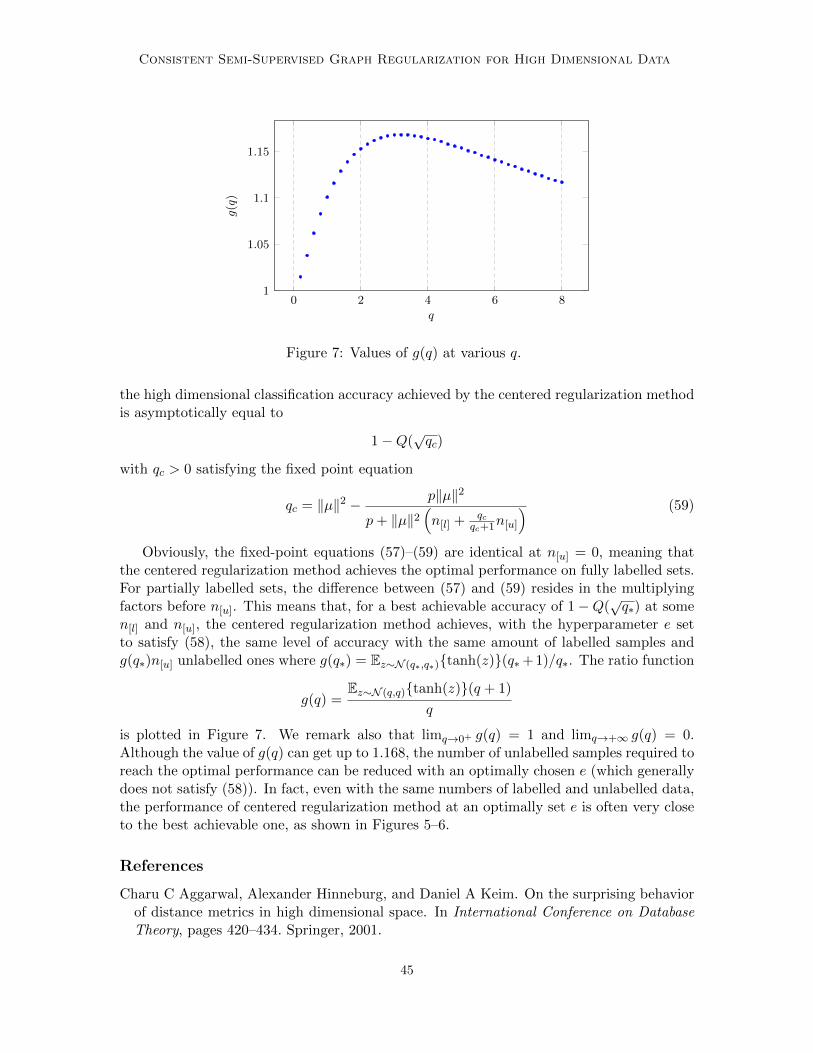
Consistent Semi-Supervised Graph Regularization for High Dimensional Data
0 2 4 6 81
1.05
1.1
1.15
q
g(q
)
Figure 7: Values of g(q) at various q.
the high dimensional classification accuracy achieved by the centered regularization methodis asymptotically equal to
1−Q(√qc)
with qc > 0 satisfying the fixed point equation
qc = ‖µ‖2 − p‖µ‖2
p+ ‖µ‖2(n[l] + qc
qc+1n[u]
) (59)
Obviously, the fixed-point equations (57)–(59) are identical at n[u] = 0, meaning thatthe centered regularization method achieves the optimal performance on fully labelled sets.For partially labelled sets, the difference between (57) and (59) resides in the multiplyingfactors before n[u]. This means that, for a best achievable accuracy of 1−Q(
√q∗) at some
n[l] and n[u], the centered regularization method achieves, with the hyperparameter e setto satisfy (58), the same level of accuracy with the same amount of labelled samples andg(q∗)n[u] unlabelled ones where g(q∗) = Ez∼N (q∗,q∗){tanh(z)}(q∗+ 1)/q∗. The ratio function
g(q) =Ez∼N (q,q){tanh(z)}(q + 1)
q
is plotted in Figure 7. We remark also that limq→0+ g(q) = 1 and limq→+∞ g(q) = 0.Although the value of g(q) can get up to 1.168, the number of unlabelled samples required toreach the optimal performance can be reduced with an optimally chosen e (which generallydoes not satisfy (58)). In fact, even with the same numbers of labelled and unlabelled data,the performance of centered regularization method at an optimally set e is often very closeto the best achievable one, as shown in Figures 5–6.
References
Charu C Aggarwal, Alexander Hinneburg, and Daniel A Keim. On the surprising behaviorof distance metrics in high dimensional space. In International Conference on DatabaseTheory, pages 420–434. Springer, 2001.
45
Mai and Couillet
Fabrizio Angiulli. On the behavior of intrinsically high-dimensional spaces: distances, directand reverse nearest neighbors, and hubness. Journal of Machine Learning Research, 18(170):1–60, 2018.
Konstantin Avrachenkov, Alexey Mishenin, Paulo Goncalves, and Marina Sokol. General-ized optimization framework for graph-based semi-supervised learning. In InternationalConference on Data Mining, pages 966–974. SIAM, 2012.
Mikhail Belkin and Partha Niyogi. Using manifold stucture for partially labeled classifica-tion. In Advances in Neural Information Processing Systems, pages 953–960, 2003.
Mikhail Belkin, Partha Niyogi, and Vikas Sindhwani. Manifold regularization: a geomet-ric framework for learning from labeled and unlabeled examples. Journal of MachineLearning Research, 7(Nov):2399–2434, 2006.
Shai Ben-David, Tyler Lu, and David Pal. Does unlabeled data provably help? worst-caseanalysis of the sample complexity of semi-supervised learning. In Conference on LearningTheory, pages 33–44, 2008.
Florent Benaych-Georges and Romain Couillet. Spectral analysis of the gram matrix ofmixture models. ESAIM: Probability and Statistics, 20:217–237, 2016.
Kevin Beyer, Jonathan Goldstein, Raghu Ramakrishnan, and Uri Shaft. When is “nearestneighbor” meaningful? In International Conference on Database Theory, pages 217–235.Springer, 1999.
Nick Bridle and Xiaojin Zhu. p-voltages: Laplacian regularization for semi-supervisedlearning on high-dimensional data. In Workshop on Mining and Learning with Graphs,2013.
Deng Cai and Xiaofei He. Manifold adaptive experimental design for text categorization.IEEE Transactions on Knowledge and Data Engineering, 24(4):707–719, 2011.
Olivier Chapelle, Bernhard Scholkopf, and Alexander Zien. Semi-supervised Learning. MITPress, 2010.
Romain Couillet and Florent Benaych-Georges. Kernel spectral clustering of large dimen-sional data. Electronic Journal of Statistics, 10(1):1393–1454, 2016.
Romain Couillet and Merouane Debbah. Random Matrix Methods for Wireless Communi-cations. Cambridge University Press, 2011.
Fabio Gagliardi Cozman, Ira Cohen, and M Cirelo. Unlabeled data can degrade classificationperformance of generative classifiers. In Flairs Conference, pages 327–331, 2002.
Ahmed El Alaoui, Xiang Cheng, Aaditya Ramdas, Martin J Wainwright, and Michael I Jor-dan. Asymptotic behavior of `p-based laplacian regularization in semi-supervised learning.In Conference on Learning Theory, pages 879–906, 2016.
46
Consistent Semi-Supervised Graph Regularization for High Dimensional Data
Noureddine El Karoui, Derek Bean, Peter J Bickel, Chinghway Lim, and Bin Yu. Onrobust regression with high-dimensional predictors. Proceedings of the National Academyof Sciences, page 201307842, 2013.
Damien Francois, Vincent Wertz, and Michel Verleysen. The concentration of fractionaldistances. IEEE Transactions on Knowledge and Data Engineering, 19(7):873–886, 2007.
Ian Goodfellow, Jean Pouget-Abadie, Mehdi Mirza, Bing Xu, David Warde-Farley, SherjilOzair, Aaron Courville, and Yoshua Bengio. Generative adversarial nets. In Advances inNeural Information Processing Systems, pages 2672–2680, 2014.
Alexander Hinneburg, Charu C Aggarwal, and Daniel A Keim. What is the nearest neighborin high dimensional spaces? In International Conference on Very Large Databases, pages506–515, 2000.
Rie Johnson and Tong Zhang. On the effectiveness of laplacian normalization for graphsemi-supervised learning. Journal of Machine Learning Research, 8(7), 2007.
Yann LeCun. The mnist database of handwritten digits. http://yann. lecun.com/exdb/mnist/, 1998.
Michel Ledoux. The Concentration of Measure Phenomenon. Number 89. American Math-ematical Soc., 2005.
Marc Lelarge and Leo Miolane. Asymptotic Bayes risk for gaussian mixture in a semi-supervised setting. arXiv preprint arXiv:1907.03792, 2019.
Cosme Louart and Romain Couillet. Concentration of measure and large random matriceswith an application to sample covariance matrices. arXiv preprint arXiv:1805.08295,2018.
Xiaoyi Mai and Romain Couillet. A random matrix analysis and improvement of semi-supervised learning for large dimensional data. Journal of Machine Learning Research,19(1):3074–3100, 2018.
Boaz Nadler, Nathan Srebro, and Xueyuan Zhou. Semi-supervised learning with the graphlaplacian: the limit of infinite unlabelled data. In Advances in Neural Information Pro-cessing Systems, pages 1330–1338, 2009.
Mauricio Flores Rios, Jeff Calder, and Gilad Lerman. Algorithms for `p-based semi-supervised learning on graphs. arXiv preprint arXiv:1901.05031, 2019.
Behzad M Shahshahani and David A Landgrebe. The effect of unlabeled samples in reducingthe small sample size problem and mitigating the hughes phenomenon. IEEE Transactionson Geoscience and Remote Sensing, 32(5):1087–1095, 1994.
Jack Sherman and Winifred J Morrison. Adjustment of an inverse matrix corresponding toa change in one element of a given matrix. The Annals of Mathematical Statistics, 21(1):124–127, 1950.
47

Mai and Couillet
Zuoqiang Shi, Stanley Osher, and Wei Zhu. Weighted nonlocal laplacian on interpolationfrom sparse data. Journal of Scientific Computing, 73(2):1164–1177, 2017.
David I Shuman, Sunil K Narang, Pascal Frossard, Antonio Ortega, and Pierre Van-dergheynst. The emerging field of signal processing on graphs: extending high-dimensional data analysis to networks and other irregular domains. IEEE Signal Pro-cessing Magazine, 30(3):83–98, 2013.
Alexander J Smola and Risi Kondor. Kernels and regularization on graphs. In LearningTheory and Kernel Machines, pages 144–158. Springer, 2003.
Ulrike Von Luxburg. A tutorial on spectral clustering. Statistics and Computing, 17(4):395–416, 2007.
Ulrike Von Luxburg, Mikhail Belkin, and Olivier Bousquet. Consistency of spectral clus-tering. The Annals of Statistics, pages 555–586, 2008.
Rudin Walter. Real and Complex Analysis. McGraw Hill Book Company, 1987.
Max A Woodbury. Inverting modified matrices. Memorandum Report, 42(106):336, 1950.
Dengyong Zhou and Bernhard Scholkopf. Regularization on discrete spaces. In Joint PatternRecognition Symposium, pages 361–368. Springer, 2005.
Denny Zhou, Olivier Bousquet, Thomas N Lal, Jason Weston, and Bernhard Scholkopf.Learning with local and global consistency. In Advances in Neural Information ProcessingSystems, pages 321–328, 2004.
Xueyuan Zhou and Mikhail Belkin. Semi-supervised learning by higher order regularization.In International Conference on Artificial Intelligence and Statistics, pages 892–900, 2011.
Xiaojin Zhu and Zoubin Ghahramani. Learning from labeled and unlabeled data with labelpropagation. 2002.
Xiaojin Zhu, Zoubin Ghahramani, and John D Lafferty. Semi-supervised learning usinggaussian fields and harmonic functions. In International Conference on Machine Learning,pages 912–919, 2003.
48