consolidation in u.s. meatpacking - usda

Consolidation in U.S. Meatpacking. By James M. MacDonald, Michael E. Ollinger,Kenneth E. Nelson, and Charles R. Handy. Food and Rural Economics Division,Economic Research Service, U.S. Department of Agriculture. Agricultural EconomicReport No. 785.

AbstractMeatpacking consolidated rapidly in the last two decades: slaughter plants became muchlarger, and concentration increased as smaller firms left the industry. We use establish-ment-based data from the U.S. Census Bureau to describe consolidation and to identifythe roles of scale economies and technological change in driving consolidation. Throughthe 1970’s, larger plants paid higher wages, generating a pecuniary scale diseconomythat largely offset the cost advantages that technological scale economies offered largeplants. The larger plants’ wage premium disappeared in the 1980’s, and technologicalchange created larger and more extensive technological scale economies. As a result,large plants realized growing cost advantages over smaller plants, and production shiftedto larger plants.

Keywords: Concentration, consolidation, meatpacking, scale economies, structuralchange.

AcknowledgmentsThe authors appreciate the reviews and suggestions of Clement Ward (Oklahoma StateUniversity), Steven Martinez and Mark Denbaly (Economic Research Service), GeraldGrinnell (Packers and Stockyards Administration), and Sang Nyugen and Arnold Reznek(Center for Economic Studies, U.S. Census Bureau).

Washington, DC 20036-5831 February 2000

Contents

Summary . . . . . . . . . . . . . . . . . . . . . . . . . . . . . . . . . . . . . . . . . . . . . . . . . . . . . . . . . .iii

Introduction . . . . . . . . . . . . . . . . . . . . . . . . . . . . . . . . . . . . . . . . . . . . . . . . . . . . . . . .1

The Setting: Developments in Meat Consumption and Livestock Production . . . . . . .3

Concentration and Consolidation in Livestock Slaughter . . . . . . . . . . . . . . . . . . . . . .7

Structural Change: Location and Plant Operations . . . . . . . . . . . . . . . . . . . . . . . . . .12

Analyzing Packer Costs: The Model . . . . . . . . . . . . . . . . . . . . . . . . . . . . . . . . . . . .17

Cattle Slaughter Cost Estimation . . . . . . . . . . . . . . . . . . . . . . . . . . . . . . . . . . . . . . .23

Hog Slaughter Cost Estimation . . . . . . . . . . . . . . . . . . . . . . . . . . . . . . . . . . . . . . . .31

Conclusions . . . . . . . . . . . . . . . . . . . . . . . . . . . . . . . . . . . . . . . . . . . . . . . . . . . . . . .37

References . . . . . . . . . . . . . . . . . . . . . . . . . . . . . . . . . . . . . . . . . . . . . . . . . . . . . . . .40

ii • USDA/Economic Research Service AER-785 • Consolidation in U.S. Meatpacking

SummaryU.S. meatpacking has been transformed in the last two decades. Far fewer meatpackersnow slaughter livestock, but their plants are much larger. Consolidation toward largerplants led to sharply increased concentration in cattle slaughter and persistent concernsover the future of competition in that industry. Hog slaughter has also consolidated, withimportant shifts toward larger plants and increased concentration.

Consolidation in slaughter features three other important elements: changes in plantlocation, product mix, and labor relations. Consolidation brought geographic changes inslaughter plants, which followed changes in the location of animal feeders. Cattleslaughter shifted to the Great Plains from the Corn Belt, while hog slaughter shiftedwest within the Corn Belt and from the Corn Belt to the Southeast.

In the early 1970’s, cattle plants were usually slaughter-only, shipping carcasses towholesalers and retailers for processing into retail products. Hog slaughter plants oftenhad extensive processing facilities for production of bacon, hams, and sausages. Today,large cattle plants, and most large hog plants, slaughter and cut up carcasses into smallercuts for shipment to wholesalers, retailers, and specialized meat processors. Productmix influences costs, and mixes vary widely across plants and over time. Because prod-uct mixes are correlated with plant size (larger cattle plants produce almost all boxedbeef, for example), their omission in models can lead to biased estimates of scaleeconomies and of the extent of technological change and productivity growth.

Our statistical analysis aims to uncover the causes of consolidation into larger plants,particularly the roles played by technological change and scale economies. Two distinctscale concepts are important: technological scale economies, relating to economies ofresource use as plant sizes increase; and pecuniary scale diseconomies, relating tochanges in labor compensation as plants grow bigger. We find extensive technologicalscale economies in hog and in cattle slaughter in 1992, and those scale economies havebecome more pronounced over time. Scale economies are small—the industry’s largestplants can deliver meat to buyers at costs 3-5 percent below those of plants only a quar-ter as big—but cost advantages extend over the entire range of plant sizes.

Wages rose sharply with plant size in the 1960’s and 1970’s, and those wage premiumsgenerated a pecuniary scale diseconomy that largely offset the cost effects of technologi-cal scale economies. But changes in labor relations accompanied industry consolida-tion—strikes, plant closings, and deunionization struggles at slaughter plants in the1980’s led to sharp declines in union membership and in average hourly wages.Moreover, the wage distribution narrowed sharply as the large plant wage premium dis-appeared. Without that pecuniary diseconomy, and with growing technological scaleeconomies, large plants realized growing cost advantages over smaller plants, and pro-duction shifted to larger plants.

We argue that slaughter concentration has increased for three reasons: (1) shifts in scaleeconomies provided larger plants with modest cost advantages; (2) aggressive pricecompetition forced prices to quickly move near the costs of the low-cost market partici-pants; and (3) slow demand growth limited the number of efficient large plants in themarket. For hogs, scale economies and strong price competition also forced small plantsto exit the industry, but modest demand growth has allowed for more plants and lowerconcentration.

AER-785 • Consolidation in U.S. Meatpacking USDA/Economic Research Service • iii

The U.S. meatpacking industry consolidated rapidly inthe last two decades, as today’s leading firms builtvery large plants and many independent packers disap-peared. Today, four firms handle nearly 80 percent ofall steer and heifer slaughter; just two decades ago,concentration was less than half as high. Although ithas not grown as rapidly, concentration in hog slaugh-ter has also increased, and today the top four firmshandle over half of all slaughter.

Consolidation raises a host of policy issues. With fewcompetitors, meatpackers may be able to reduce pricespaid to livestock producers, and they may be able toraise meat prices charged to wholesalers and retailers.Indeed, livestock prices have been at the center of sev-eral recent lawsuits, congressional hearings, andFederal investigations.1

Related consolidation has occurred in livestock pro-duction: large cattle feedlots and hog farms accountfor high and growing shares of livestock sales, andtheir expansion is closely linked to the presence oflarge slaughter facilities nearby. Consolidation in pro-duction may worsen water pollution and odor prob-lems, and has spurred intense debate over environmen-tal policies in more than 20 States.

Slaughterhouses have always been risky places towork, and plants today rely on large workforces ofimmigrant workers to operate slaughter and fabricationlines.2 As a result, slaughter plants frequently attractthe scrutiny of job safety regulators and immigrationauthorities. Finally, a concentrated system of largeplants and livestock producers may require a differentset of regulatory strategies for reaching food safety

goals than would an industry with many small produc-ers and slaughter plants (MacDonald et al., 1996).

Policy issues tend to address the effects of consolida-tion, whereas this report aims to assess causes. We usea unique and valuable data set to describe and toexplain consolidation.3 In particular, we examine howseveral innovations may have reduced slaughter costsand promoted consolidation among slaughter firms.Changes in slaughter plant technology may have creat-ed scale economies, altered the mix of slaughter plantproducts, and changed the location and operations ofcattle and hog producers (which may affect the opti-mal location, scale, and operations of slaughter plants).In addition, changes in labor relations have led toreductions in wages and may have created additionalscale economies. We believe that it is crucial to under-stand the causes of slaughter industry consolidationwhen fashioning appropriate public policies to dealwith its effects.

The report relies on a unique data source, the U.S.Census Bureau’s Longitudinal Research Database(LRD). The LRD details the records of individualestablishments reported in the census of manufactures,for the years 1963, 1967, 1972, 1977, 1982, 1987, and1992 (1997 census data will be processed too late forthis report). The files detail the physical quantities anddollar sales of many different products sold fromslaughter plants, the physical quantities and prices paidfor material inputs, and employment and averagewages for each establishment. The files also note own-ership and location for each establishment. Becausethe LRD covers several censuses, we can make com-parisons across plants at a point in time, as well asover time.

AER-785 • Consolidation in U.S. Meatpacking USDA/Economic Research Service • 1

Chapter 1

Introduction

1 For a summary, see Feder (1995), or the report of the Secretaryof Agriculture’s Advisory Committee on AgriculturalConcentration (1996).

2 For a discussion of the transformation of rural communities, andthe associated impacts on job injury risks and immigration rules,see Hedges and Hawkins (1996).

3 A companion report (Ollinger et al., 1999) analyzes the poultrysector.

While researchers can access individual LRD estab-lishment records for research purposes, they may notdivulge information on an individual plant or firm, andmay publish only aggregated information. This reporttherefore presents aggregated statistical data and the

coefficients from regression analyses covering hun-dreds and, in most cases, thousands of establishmentrecords. Any references to specific company or plantnames are based on publicly available records, and noton any census source.

2 • USDA/Economic Research Service Consolidation in U.S. Meatpacking • AER-785

Cattle and hog slaughter plants operate in conjunctionwith meat buyers and with livestock suppliers. Overthe years covered by this study (1963-92), the eco-nomics of slaughter industries have been affected bysome important developments in meat consumptionpatterns and in methods of livestock supply. 4

Changes in Meat ConsumptionMeat consumption patterns changed markedly in thelast quarter century, shifting from red meats, and par-ticularly beef, to poultry (table 2-1). Beef consumptiondropped from 84.7 pounds per person in 1971-75 to66.3 pounds by 1991-95. Over the same period, percapita pork consumption changed little from 51.9pounds in 1971-75 to 52.1 pounds in 1991-95. In con-trast, poultry consumption rose sharply. Per capitachicken consumption nearly doubled, from 36 poundsin the early 1970’s to almost 70 pounds in 1995, whileturkey consumption (not shown) jumped from 8pounds in 1970 to 18 pounds in 1995.

The shifts derive from trends in relative prices amongmeats, health concerns, and the development of manynew poultry products. But the changes forced slaugh-ter industries to adapt. With declining per capita con-sumption, growth in beef demand, and consequentlygrowth in demand for slaughter cattle, could comeonly from growth in population and in exports.

The U.S. population grew about 1 percent per yearduring 1970-95 or, compounded, 28 percent over theentire period. Coupled with declining per capita con-

sumption and only a slight increase in net beefexports, total U.S. demand for beef showed littlegrowth.5 But changes in animal production meant thatconstant beef demand could be met with fewer ani-mals. Beef yields rose to almost 700 pounds per car-cass in the early 1990’s from just over 600 pounds twodecades before; consequently, cattle slaughter (num-bers) fell by 13 percent between the late 1970’s andthe early 1990’s.

Hog yields grew slightly during the period, as did netpork exports, while per capita consumption showed lit-tle change. The net effect was modest growth (15 per-cent) in annual hog slaughter over the two decades;that is, demand for slaughter hogs grew, but by lessthan 1 percent per year.

Poultry stands in stark contrast. Growth in broiler size(average meat yields from a broiler grew by nearly 20percent) also limited the growth in demand for slaugh-ter livestock. But growth in population, exports, andper capita consumption caused broiler slaughter tojump from 2.9 billion animals a year in the early1970’s to 6.6 billion in the early 1990’s.

Later chapters will show that dramatic structuralchanges affected each of the slaughter industries dur-ing the period, as production shifted to larger plants.But those shifts occurred in the face of widely varyingeconomic environments. In cattle, production shiftedto larger plants in the face of declining demand forslaughter cattle; the result was sharp declines in plantnumbers and sharp increases in concentration. By con-trast, shifts to larger plants in poultry slaughter accom-


Chapter 2

The Setting Developments in Meat Consumption

and Livestock Production

4 We emphasize the developments that affect slaughter plant eco-nomics. More complete descriptions of meat consumption andlivestock production can be found in Crom (1988), McBride(1997), USDA (1995), and Putnam and Allshouse (1997).

5 Net exports refer to exports minus imports, measured in quanti-ties (rather than in dollar values). During the period, net exportsgrew from -7 to -4 percent; that is, exports grew faster thanimports, creating some net demand growth for U.S. beef.

modated growing demand, so fewer plants exited andconcentration changed little.6 With slow but positivedemand growth for hogs, shifts to larger plants result-ed in plant exits and some increase in concentration,but nothing like the sharp consolidation in cattleslaughter.

The Supply Chain: Cattle Production

Cattle slaughter plants usually specialize in one of twotypes of cattle. Of the 35.7 million cattle slaughteredin 1996, 28.3 million were steers and heifers, while therest were cows and bulls. Plants specialize because theanimals have different shapes that require different set-tings for slaughter line equipment, and because theanimals provide different meat products. Steers andheifers are fed a concentrated diet of corn rations

before slaughter, producing a more marbled cut of beefthat is preferred for taste. Cows, fed on grass and for-age, produce leaner meat that is usually mixed withtrimmings from steer and heifer carcasses to produceground beef.

Cows sometimes move through feedlots before goingto slaughter plants, but more often move directly toplants from dairy farms and beef cow-calf operations.Because of that, cow and bull sales and slaughterplants are widely distributed across the country. Texasaccounted for 12 percent of the Nation’s 1996 cow andbull sales, and 15 other States, from all regions of thecountry, each accounted for at least 1 percent. Becausesales are distributed over a wide geographic area,slaughter plants tend to be smaller than steer andheifer plants (larger plants would require uneconomi-cally large catchment areas).

The animals that steer and heifer plants eventually pur-chase are first calved on a wide variety of farm opera-tions spread across the country. Most producers arequite small. Calves are usually weaned from cowswhen they weigh about 400 pounds. Of those that areto be grown out for beef, 80 to 90 percent are placed


Table 2-1—From meat demand to livestock slaughter

Variables driving Annual averagelivestock demand 1971-75 1976-80 1981-85 1986-1990 1991-95

Percentage increase

U.S. population growth 1.04 1.07 0.93 0.94 1.04

Per capita consumption: Pounds

Beef 84.7 85.6 78.1 72.5 66.3Pork 51.9 50.1 51.8 50.4 52.1Chicken 36.8 42.8 48.3 55.8 66.4

Net meat exports: Percent of domestic supply

Beef -7.0 -7.7 -6.4 -5.7 -4.0Pork -2.3 -1.3 -3.6 -5.3 -1.7Chicken +1.3 +4.8 +3.9 +4.9 +8.7

Average carcass size: Dressed weight, pounds

Cattle 612 615 632 666 699Hogs 169 170 173 178 182Broilers 3.74 3.88 4.10 4.31 4.45

Commercial slaughter: Million animals

Cattle 36.6 38.3 36.3 35.0 33.3Hogs 81.3 82.7 86.2 84.5 93.0Broilers 2,889 3,575 4,198 5,223 6,580

Sources: Putnam and Allshouse, 1997; USDA, ERS, 1995.

6 Turkey slaughter also increased sharply, for similar reasons.Annual slaughter numbers in the early 1990’s were 130 percentabove those of two decades earlier, following sharp increases inper capita consumption and more modest growth in population andexports. Meat yields from turkeys rose 20 percent.

in growing operations (many of which are integratedwith cow-calf operations), where they add weightwhile pasturing on grass and roughage. Feeder cattleoften move among growing operations, and to manydifferent locations around the country, as pasture andforage conditions vary.

Feeder cattle commonly move to feedlots when theyweigh between 500 and 750 pounds. The animalsremain in feedlots until they reach market weights of950 to 1,250 pounds, and are sold to slaughter plants.Feedlots, and hence steer and heifer plants, are geo-graphically concentrated. According to an annualUSDA survey, 75 percent of all packer purchases ofsteers and heifers in 1996 came from just five States inthe Great Plains—Colorado, Nebraska, Kansas,Oklahoma, and Texas (USDA, 1998).

Feedlots cover a wide range of sizes, but sales to pack-ers are increasingly dominated by large commercialfeedlots in which almost all feed is purchased (ratherthan grown onsite), almost all labor is hired, and theanimals are confined to a relatively small area. A 1992USDA survey of the largest steer and heifer plantsshows they bought cattle from many different sellers—19,395 of them.7 Most sellers (89 percent) were smallfarmer-feedlots—seasonal operations with capacitybelow 1,000 head, which are part of a diversified farmbusiness. But, on average, the survey’s farmer-feedlotssold less than 200 cattle each in 1992, in 2 to 3 trans-actions, and together those sellers accounted for only14 percent of the cattle purchased in the survey.

Packers purchased far more animals from very largecommercial feedlots; 150 sellers in the 1992 survey soldover 32,000 cattle each, and together accounted for 43percent of all cattle purchased by the packers. Theselarge commercial feedlots sold an average of 65,000animals each in 1992, in over 400 differenttransactions.8 Almost all were located in the GreatPlains.

In the mid-1970’s, large commercial feedlots accountedfor less than a quarter of total steer and heifer sales.Since then, their growth has paralleled that of largeslaughter plants. Technological innovations—such asfeed additives, computerized onsite feedmills and feed-ing operations, and improved transportation—haveheightened economies of size in cattle feeding (Gloverand Southard, 1995). By building a large slaughter plantamong a network of large feedlots, plant managers canensure a steady supply of animals and can maintainhigh capacity utilization throughout the year. The eco-nomics of slaughter plant operation and pricing areintertwined with large feedlot operations and pricing.

The Supply Chain: Hog Production

Meatpackers usually purchase hogs locally—within150 miles of the slaughterhouse—so facilities conse-quently locate near hog farms, much as cattle slaughterplants locate near cattle feedlots. But hog finishing isnot as geographically concentrated as cattle feeding.While the five largest cattle-feeding States form a con-tiguous region accounting for three-quarters of fed cat-tle sales, the five largest hog-finishing States form twodistinct regions (the Western Corn Belt and the NorthCarolina-Virginia area), and together account for justover 60 percent of hogs marketed to slaughterhouses.

Hog production falls into several distinct phases: pro-duction of breeding stock, feeder pig production, andfinishing. While hog producers usually maintain theirown female breeding stock, most boars are supplied byspecialized commercial breeders. In the next twostages, some producers specialize in either feeder pigproduction or finishing, with hogs transferred betweenthe two stages in a commercial transaction. But mostoperations are farrow-to-finish.

Hog production at the latter two stages has undergone adramatic and ongoing consolidation, represented by ashift toward larger production establishments andtoward long-term contractual arrangements among theproduction stages and between production and slaugh-ter. In 1978, 96 percent of all hog farms sold less than1,000 head, and together accounted for just under two-thirds of all hog marketings. By 1997, 77 percent of allfarms sold less than 1,000 head, but they accounted foronly 5 percent of marketings (Lawrence, Grimes, andHayenga, 1998). The very largest farms, those sellingmore than 50,000 head a year, handled 37 percent of all


7 Those plants slaughtered 23.1 million cattle, 87.6 percent of allcommercial steer and heifer slaughter in that year. The relevantsurvey data were collected by USDA’s Grain Inspection, Packersand Stockyards Administration (GIPSA), as summarized in TexasAgricultural Market Research Center (1996).

8 Another 144 sellers, which each sold more than 16,000 cattle tothe largest plants, accounted for 3.3 million head. The remaining28.8 percent of steer and heifer sales came from 1,873 smallercommercial feedlots.

hog marketings in 1997, up from 7 percent only adecade before. Of those producers, 18 sold at least500,000 head in 1997, and those accounted for nearlyone-quarter of all marketings. Very large hog producersare highly specialized, purchasing feed rather thangrowing it, and are frequently linked to slaughterhousesthrough contractual agreements or common ownership.

With hog production increasingly divorced from cornand soybean production, large operations could locatevirtually anywhere in the country. Many of the verylarge hog farms have located outside of the traditionalregion of hog production—the Corn Belt States ofMinnesota, Iowa, and Illinois—which includes aboutone-third of all U.S. hog farms and over 40 percent ofhog marketings. But only 16 percent of the region’shog marketings come from farms selling at least 5,000head—most marketings come from farms sellingbetween 500 and 5,000 head per year. By contrast, inthe newly emerging Southeastern hog productionregion (North and South Carolina and southernVirginia), nearly 80 percent of hog marketings comefrom farms that sell more than 5,000 head each.Similarly, very large producers underlie the expansionof the hog industry in Oklahoma and proposals forexpansion in Utah and other nontraditional States.Large hog operations can bring odor and water prob-lems, and may threaten small operations; as a result,

hog farm location has become a political and regulato-ry battleground in many States (Johnson, 1998;Drabenstott, 1998). Location of new hog productionfacilities may shift significantly in the near future,depending on how these issues are resolved.

Economies of size can account for much of the growthin hog farm size (McBride, 1995). Production costsper hog drop sharply as annual marketings increase to1,000 head, and continue to decline, but more slowly,as size increases past that level. In turn, unit produc-tion costs decline largely because of improved feedefficiency and labor productivity on larger hog farms.

Economies of scale in hog and cattle slaughteremerged in the 1980’s and 1990’s. The largest slaugh-ter plants in 1992 held significant cost advantages oversmaller plants. Growth in slaughter plant size may berelated to shifts in the size and location of hog produc-ers and cattle feeders. Economies of scale in slaughterapply only if plant operators have access to an assuredsteady supply of cattle or hogs; large plants quicklylose any cost advantages if they cannot operate nearfull capacity. By locating among a network of largeproducers, and by forming long-term relationshipswith those producers, slaughter plants may reduce therisks asociated with building and operating largeplants.


Concentration in cattle slaughter increased dramatical-ly in the last two decades, and three firms now domi-nate the industry. Market concentration in hog, chick-en, and turkey slaughter is not particularly high whencompared with other manufacturing industries, but hasincreased over the years. Large plants now dominateproduction in all major slaughter sectors, and consoli-dation among large plants over the past two decades isa major cause of increased concentration.

ConcentrationThe four-firm concentration ratio measures the shareof an industry’s output held by the four largest produc-ers in the industry.9 Changes in four-firm ratios arewidely used as summary indicators of structuralchange.

Using Census Bureau data, table 3-1 reports concen-tration ratios for cattle, hogs, chickens, and turkeys.The ratios measure the four largest firms’ share of thedollar value of shipments from plants in each slaughterclass.10

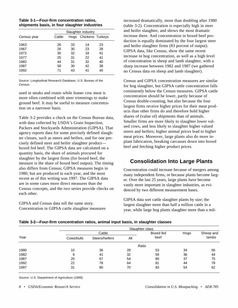
Four-firm concentration in cattle slaughter remainedstable from 1963 through 1977, then rose from 25 per-

cent in 1977 to 71 percent in 1992 (table 3-1). TheCensus Bureau publishes four-firm concentrationratios for about 1,000 different product classes, andmany of the series go back to 1947. The change in cat-tle slaughter concentration is unique: no other productclass shows as dramatic an increase in any 15-yearperiod.

Concentration in hog slaughter remained stable from1963 through 1987, but then increased sharplybetween 1987 and 1992. Concentration in chickenslaughter rose sharply from 1977 to 1987, but hassince remained stable. Similarly, turkey slaughterbecame much more concentrated between 1963 and1972, and then stabilized (table 3-1). Of the four class-es, only cattle could be described as having unusuallyhigh concentration today, when compared with othermanufacturing classes.11

Census data are subject to two potential problems.First, they measure concentration as the value of plant(establishment) shipments. But suppose that a firmoperated a plant that only slaughtered cattle and thenshipped the carcasses to a second plant that bothslaughtered cattle and also cut up carcasses into boxedbeef. The Census approach would count the value ofshipments from both the slaughter-only plant and thefabrication plant. But since fabrication plant shipmentsalready include the value of shipments from theslaughter-only plant, the Census measure double-counts shipments among slaughter plants, and thisapproach may overstate the value of shipments fromthe combined firm and thus exaggerate industry con-centration. Second, Census measures may be toobroad. Cattle plants specialize within species; thelargest plants slaughter only steers and heifers, whileother plants specialize in cows and bulls. Not only dothe plants use different techniques, but the meat out-puts are not ready substitutes: steer and heifer meat is


Chapter 3

Concentration and Consolidation in Livestock Slaughter

9 There are many potential concentration measures. The four-firmratio is easy for statistical agencies to compute and provides confi-dentiality to individual firms. For those reasons, the measure hasfor several decades been calculated for many industries by Federalstatistical agencies.

10 The classes are defined by the Standard Industrial Classification(SIC), a hierarchical coding for products and establishments in theeconomy. Establishments that primarily process food products areassigned to the two-digit SIC code “20”; those food processorsthat specialize in meat slaughter and processing are assigned to thethree-digit class “201.” Establishments that slaughter any live cat-tle, hogs, horses, or sheep and lambs are then assigned to the four-digit industry “2011”(those that process or slaughter poultry areassigned to “2015”). Finally, slaughter products from these plantsare assigned to five-digit product classes: “20111” for cattle,“20114” for hogs, “20151” for chickens, and “20153”for turkeys.Our concentration measures are based on shipments from estab-lishments assigned to the five-digit slaughter product classes.

11 About 10 percent of U.S. manufacturing industries are moreconcentrated than cattle slaughter, while the other three slaughterclasses are close to the mean for manufacturing.

used in steaks and roasts while leaner cow meat ismore often combined with steer trimmings to makeground beef. It may be useful to measure concentra-tion on a narrower basis.

Table 3-2 provides a check on the Census Bureau data,with data collected by USDA’s Grain Inspection,Packers and Stockyards Administration (GIPSA). Thatagency reports data for some precisely defined slaugh-ter classes, such as steers and heifers, and for one pre-cisely defined steer and heifer slaughter product—boxed fed beef. The GIPSA data are calculated on aquantity basis, the share of animals procured forslaughter by the largest firms (for boxed beef, themeasure is the share of boxed beef output). The timingalso differs from Census; GIPSA measures begin in1980, but are produced in each year, and the mostrecent as of this writing was 1997. The GIPSA dataare in some cases more direct measures than theCensus concepts, and the two series provide checks oneach other.

GIPSA and Census data tell the same story.Concentration in GIPSA cattle slaughter measures

increased dramatically, more than doubling after 1980(table 3-2). Concentration is especially high in steerand heifer slaughter, and shows the most dramaticincrease there. And concentration in boxed beef pro-duction is equally dominated by the four largest steerand heifer slaughter firms (83 percent of output).GIPSA data, like Census, show the same recentincrease in hog concentration, as well as a high levelof concentration in sheep and lamb slaughter, with asharp increase between 1982 and 1987 (we gatheredno Census data on sheep and lamb slaughter).

Census and GIPSA concentration measures are similarfor hog slaughter, but GIPSA cattle concentration fallsconsistently below the Census measures. GIPSA cattleconcentration should be lower, partly because ofCensus double-counting, but also because the fourlargest firms receive higher prices for their meat prod-ucts than other firms do and therefore hold highershares of (value of) shipments than of animals.Smaller firms are more likely to slaughter lower val-ued cows, and less likely to slaughter higher valuedsteers and heifers; higher animal prices lead to highermeat prices. Moreover, large plants also do more in-plant fabrication, breaking carcasses down into boxedbeef and fetching higher product prices.

Consolidation Into Large PlantsConcentration could increase because of mergers amongmany independent firms, or because plants become larg-er. Over the last 25 years, large plants have becomevastly more important in slaughter industries, as evi-denced by two different measurement bases.

GIPSA data sort cattle slaughter plants by size; thelargest slaughter more than half a million cattle in ayear, while large hog plants slaughter more than a mil-


Table 3-1—Four-firm concentration ratios, shipments basis, in four slaughter industries

Slaughter industryCensus year Cattle Hogs Chickens Turkeys

1963 26 33 14 231967 26 30 23 281972 30 32 18 411977 25 31 22 411982 44 31 32 401987 58 30 42 381992 71 43 41 45

Source: Longitudinal Research Database, U.S. Bureau of theCensus.

Table 3-2—Four-firm concentration ratios, animal input basis, in slaughter classes

Slaughter classCattle Boxed fed Hogs Sheep and

Year Cows/bulls Steers/heifers All beef lambs

Ratio1980 10 36 28 53 34 561982 9 41 32 59 36 441987 20 67 54 80 37 751992 22 78 64 81 44 781997 31 80 70 83 54 62

Source: U.S. Department of Agriculture (1999).

lion. Notions of “large” can change over time; theagency did not separately report cattle plants thatslaughtered more than a million animals until 1987; by1997, 14 plants were in that newly established category.

The emergence of large plants is quite striking. In1977, 84 percent of all steer and heifer slaughteroccurred in plants that slaughtered less than half a mil-lion a year. By 1997, plants in that category saw theirshare drop to 20 percent, while 63 percent of slaughteroccurred in plants that slaughtered more than a millionsteers and heifers (table 3-3). In hog slaughter, largeplants handled 38 percent of all slaughter in 1977, but88 percent by 1997.

Census data report on the value of shipments by employ-ment size of firm. We use that basis here, to maintainsome comparability to other Census industries. Wedefine large plants as those with at least 400 employees,in order to meet Census confidentiality rules.

Census measures are not directly comparable with theGIPSA series, but they show the same trend. Large-plant shares in all four categories (cattle, hogs, chick-ens, and turkeys) increased dramatically during 1963-92 (table 3-4). GIPSA data generally show a muchsharper increase than Census data. Since the GIPSAdata are based on the number of animals, while Censusdata use an employment cutoff, the contrast suggests asubstantial increase in labor productivity at largeplants. Each source shows sharply increased concen-tration in cattle slaughter, and a more recent concentra-tion in hogs.

ConclusionThe evidence shows a dramatic consolidation ofslaughter in large plants in all four animal classes.That pattern suggests that scale economies may beimportant in slaughter industries, and that somethinghappened to make scale economies more important inrecent years. Later in this report, we explore thoseissues with statistical cost models. We estimate theextent of scale economies in slaughter, and identify agrowing importance of scale economies.

A second interesting pattern stands out. Dramatic con-solidation among large plants in four slaughter indus-tries led to dramatic concentration increases in justone—cattle slaughter. Changes in concentration havebeen far more modest in hog, chicken, and turkeyslaughter. Demand growth has likely played a rolehere. As chapter 2 shows, per capita poultry consump-tion has grown sharply in the United States over thelast two decades, while per capita pork consumptionhas grown modestly and beef consumption has been


Table 3-3—Percent of animals slaughtered in large plants

Report year Slaughter classes, and size cutoff1

All cattle Steers/heifers Cows/bulls Hogs Sheep/lambs

(>500,000) (>500,000) (> 1 million) (>150,000) (>1 million) (>300,000)

Percent1977 12 16 nr 10 38 421982 28 36 nr 15 59 731987 51 63 31 20 72 841992 61 76 34 38 86 741997 65 80 63 57 88 71

1 The size cutoff, in parentheses, refers to the number of animals slaughtered annually.nr = not reported.Source: U.S. Department of Agriculture (1999).

Table 3-4—Share of industry value of shipments inlarge plants (> 400 employees)

Slaughter industry

Census year Cattle Hogs Chickens Turkeys

Percent

1963 31 66 d d1967 29 63 29 161972 32 62 34 151977 37 67 45 291982 51 67 65 351987 58 72 76 641992 72 86 88 83

d = cannot be disclosed, due to confidentiality concerns.Source: Longitudinal Research Datafile, U.S. Bureau of the Census.

flat. When combined with modest export and popula-tion growth, the cattle slaughter industry has facedvery slow to declining demand growth. When setagainst shifts to large plants, the results should beincreased concentration.

Appendix 3A: Sources of Establishment Data for

Livestock SlaughterThree Federal agencies—USDA's Grain Inspection,Packers and Stockyards Administration (GIPSA) andFood Safety and Inspection Service (FSIS), and theBureau of the Census (U.S. Department ofCommerce)—report data on animal slaughter. Eachhas different goals, which lead to different methods ofdata collection. In general, the three agencies reportdata from the same set of large and medium-sizedplants, but differ substantially in their coverage of verysmall plants.

GIPSA is a regulatory agency whose mission is toguard against anticompetitive, deceptive, and fraudu-lent practices in the pricing and movement of livestockand meat products. FSIS is also a regulatory agency,whose primary activity is inspection of meat and poul-try sold in interstate commerce, primarily to ensureanimal and human health. The Census Bureau, as partof its census of manufactures, aims to measure theeconomic characteristics—such as sales, costs, andemployment—of meat and poultry industries.Different agency missions lead to different reportingrequirements.

GIPSA data are based on reports from slaughteringmeatpackers operating in commerce in the UnitedStates. Small packers (who purchase $500,000 or lessof livestock annually) are exempt from GIPSA report-ing requirements. We can assume that plants thatslaughter fewer than 10 steers or 90 hogs a week(roughly) are omitted from GIPSA reports, as areplants that do not purchase livestock for slaughter butinstead perform custom slaughter services for live-stock owners. For reporting plants, GIPSA obtainsdata on livestock volumes by plant, species, and loca-tion of seller.

All plants that slaughter or process meat to be sold ininterstate commerce are subject to Federal safetyinspection. FSIS reports therefore cover a wide rangeof plant sizes, but do not cover plants that sell only

within States, exempting many very small plants butstill capturing more small plants than GIPSA. In sup-port of its regulatory responsibilities, FSIS obtainsuseful summary data on livestock volumes by plantand species.

The census of manufactures reports data from all plantswhose primary business is manufacturing. As a result,facilities that do some animal slaughter, but that areprimarily in retailing or wholesaling or other nonmanu-facturing activities, are not reported in the census ofmanufactures. Of those whose primary business ismanufacturing, the Bureau assigns all plants that doany red meat slaughter to SIC code 2011, meatpacking,even if they are primarily active in meat processing.Plants that only process meat, conducting no slaughteron premises, are assigned to SIC code 2013, meat pro-cessing. The Bureau has an additional small businessexemption for some data: plants with fewer than 20employees are not required to make detailed reports.The Census Bureau counts those plants, but does notobtain detailed information on slaughter volume fromthem. Thus, Census procedures likely count more smallplants than GIPSA, but exempt more volume.

How do the three sources compare? In general, aggre-gated numbers are quite similar, because the threesources cover a common set of large plants. For exam-ple, appendix table 3-1 compares total slaughter vol-umes for 1992. USDA's National AgriculturalStatistics Service (NASS) estimates the total commer-cial slaughter of cattle and hogs. Federally inspectedslaughter totals (FSIS) account for 97.6 percent oftotal commercial cattle and hog slaughter—the differ-ence presumably slaughter in State-inspected plants.GIPSA totals sum to 94.9 percent of total commercialcattle slaughter, and 96.5 percent of total commercialhog slaughter, with the differences reflecting slaughterby exempt entities—very small plants. Finally, Censustotals, which exempt establishments primarily outsideof manufacturing and exempt very small plants fromdetailed reporting of species volume, capture 94.5 per-cent of commercial cattle slaughter and 91 percent ofhog slaughter.

The three series can disagree widely on plant counts,because very small plants make up substantial sharesof any plant count. For example, all three agenciesreport substantial declines in plant numbers between1977 and 1992 (appendix table 3-2): Census red meatslaughter plants declined by 46.4 percent, GIPSA by

10 • USDA/Economic Research Service Consolidation in U. S. Meatpacking • AER-785

43.1 percent, and FSIS by 33.1 percent. But theabsolute levels differ sharply. The Census reports overtwice as many plants as GIPSA does, and is mostlyhigher than FSIS counts. This is because the Censusapproach counts more small plants than GIPSA doeswhile its exempt plants (those outside of manufactur-ing that may do some slaughter) may overlap with theplants that FSIS does not count (those that slaughterbut do not sell in interstate commerce).

Comparisons are more difficult at the species level.GIPSA and FSIS count plants as cattle slaughter facili-ties if they slaughter any cattle, even if they primarilyslaughter other species such as hogs. They then reportthe same facilities as hog slaughter plants if theyslaughter any hogs. Census counts exempt very smallplants from reporting livestock volumes, so they arenot captured in counts of cattle or hog slaughter plants.Furthermore, for purposes of counting plants, wecount a plant as a cattle (hog) slaughter plant only ifits primary activity is cattle (hog) slaughter. That is,we count Census plants only once, while GIPSA andFSIS plants may be counted several times when sum-ming slaughterers of particular species.

Thus, Census reports the fewest plants (appendix table3-3) because it does not count very small plants andbecause we assign a plant to one species only. GIPSAcounts are higher because that agency assigns plants tomore than one category and because it probably countsmore very small plants. Finally, FSIS reports on morevery small plants, for these purposes, than either of theother agencies, and also assigns plants to more thanone species category. Still, the three sources all showlarge declines in the number of slaughter plants overtime.

The empirical analyses in this report are primarilybased on data reported by the Census Bureau estab-lishments in appendix table 3-3 (exceptions are someaggregated data from GIPSA records). We hence omitmany very small establishments. However, thoseestablishments account for very small shares of indus-try production.


Appendix table 3-1—Slaughter volumes, by reporting system (1992)

Cattle Hogs

Plant category Number Percent of commercial Number Percent of commercial

All commercial plants 32,874 100.0 94,889 100.0Federally inspected 32,094 97.6 92,611 97.6Reporting to GIPSA 31,200 94.9 91,550 96.5Census, SIC 2011 31,068 94.5 86,308 91.0

Sources: U.S. Department of Agriculture (1997), and Longitudinal Research Database, U.S. Bureau of the Census.

Appendix table 3-2—Livestock slaughter establish-ments, by reporting system, 1977-96

Reporting system

Year GIPSA Federally Census, inspected SIC 2011

Number

1977 1,000 1,682 2,5901982 884 1,688 1,7801987 722 1,483 1,4341992 569 1,125 1,3871996 418 988 nr

Sources: U.S. Department of Agriculture (1997), and LongitudinalResearch Database, U.S. Bureau of the Census.

Appendix table 3-3—Slaughter plants, by speciesand by reporting system

Cattle Hogs

Year Census GIPSA FSIS Census GIPSA FSIS

Number1963 1,817 nr nr 1,410 nr nr1967 1,031 nr nr 797 nr nr1972 782 920 nr 575 594 nr1977 598 814 1,568 404 469 1,2311982 391 632 1,506 325 466 1,3441987 265 474 1,317 214 352 1,1821992 215 342 971 182 300 9211996 nr 274 812 nr 232 770

nr = not reportedCensus refers to Census of Manufactures (“cattle” covers plants pri-marily producing in SIC 20111, while “hogs” covers plants primarilyproducing in SIC 20114).Sources: U.S. Department of Agriculture (1997), and LongitudinalResearch Database, U.S. Bureau of the Census.

Industry consolidation involves more than changes inconcentration and plant sizes. Other dramatic changesaffect product and input mix, industry location, and theorganization and compensation of workforces atslaughter plants.

Today’s largest cattle slaughter plants operate in a lim-ited geographic area: Nebraska, Kansas, easternColorado, and the Texas Panhandle. These plants typi-cally slaughter 4,000 to 5,000 cattle a day, and alsofabricate carcasses into smaller cuts, which are thendistributed directly to wholesalers and retailers.

In the past, large hog plants also processed carcassesinto hams, bacon, other cured products, and sausages.Today, they are more likely to simply slaughter hogsand cut up the carcasses, selling the meat to processingplants. Hog slaughter is not as geographically concen-trated as cattle. New plants are tied to large hog feed-ing operations, and as those have spread through sev-eral rural areas of the country, so have slaughterplants.

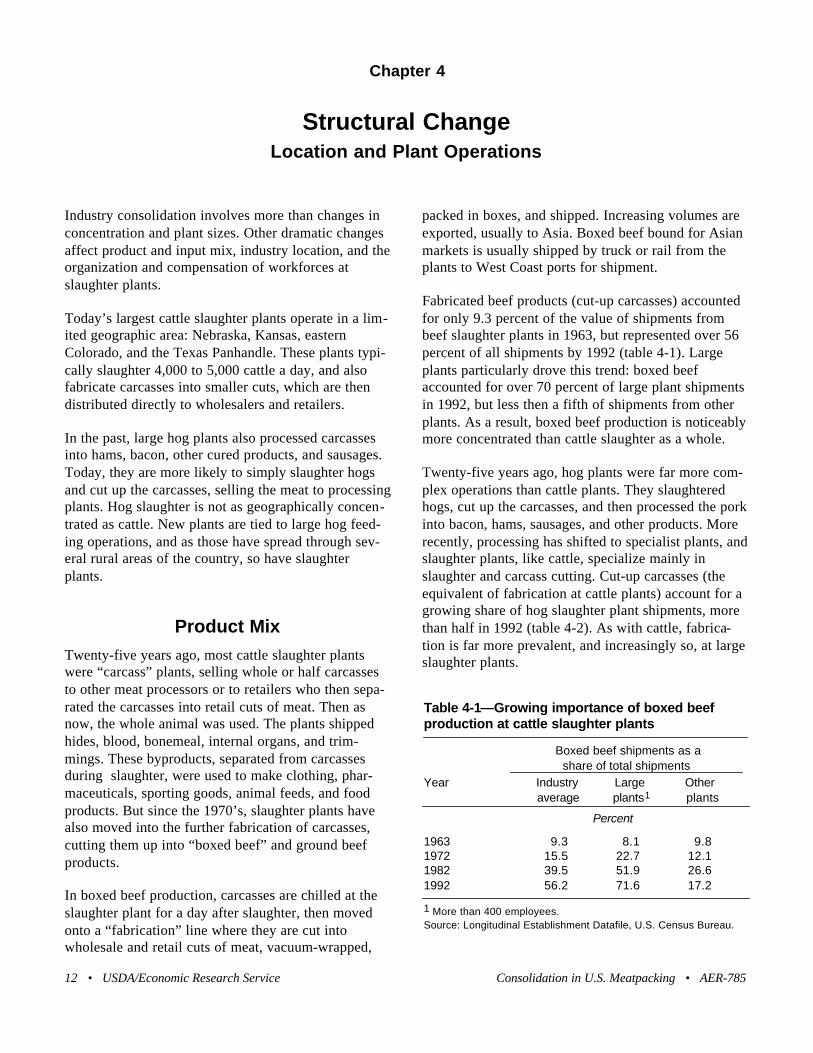
Product MixTwenty-five years ago, most cattle slaughter plantswere “carcass” plants, selling whole or half carcassesto other meat processors or to retailers who then sepa-rated the carcasses into retail cuts of meat. Then asnow, the whole animal was used. The plants shippedhides, blood, bonemeal, internal organs, and trim-mings. These byproducts, separated from carcassesduring slaughter, were used to make clothing, phar-maceuticals, sporting goods, animal feeds, and foodproducts. But since the 1970’s, slaughter plants havealso moved into the further fabrication of carcasses,cutting them up into “boxed beef” and ground beefproducts.

In boxed beef production, carcasses are chilled at theslaughter plant for a day after slaughter, then movedonto a “fabrication” line where they are cut intowholesale and retail cuts of meat, vacuum-wrapped,

packed in boxes, and shipped. Increasing volumes areexported, usually to Asia. Boxed beef bound for Asianmarkets is usually shipped by truck or rail from theplants to West Coast ports for shipment.

Fabricated beef products (cut-up carcasses) accountedfor only 9.3 percent of the value of shipments frombeef slaughter plants in 1963, but represented over 56percent of all shipments by 1992 (table 4-1). Largeplants particularly drove this trend: boxed beefaccounted for over 70 percent of large plant shipmentsin 1992, but less then a fifth of shipments from otherplants. As a result, boxed beef production is noticeablymore concentrated than cattle slaughter as a whole.

Twenty-five years ago, hog plants were far more com-plex operations than cattle plants. They slaughteredhogs, cut up the carcasses, and then processed the porkinto bacon, hams, sausages, and other products. Morerecently, processing has shifted to specialist plants, andslaughter plants, like cattle, specialize mainly inslaughter and carcass cutting. Cut-up carcasses (theequivalent of fabrication at cattle plants) account for agrowing share of hog slaughter plant shipments, morethan half in 1992 (table 4-2). As with cattle, fabrica-tion is far more prevalent, and increasingly so, at largeslaughter plants.


Chapter 4

Structural Change Location and Plant Operations

Table 4-1—Growing importance of boxed beef production at cattle slaughter plants

Boxed beef shipments as a share of total shipments

Year Industry Large Other average plants1 plants

Percent

1963 9.3 8.1 9.81972 15.5 22.7 12.11982 39.5 51.9 26.61992 56.2 71.6 17.2

1 More than 400 employees.Source: Longitudinal Establishment Datafile, U.S. Census Bureau.

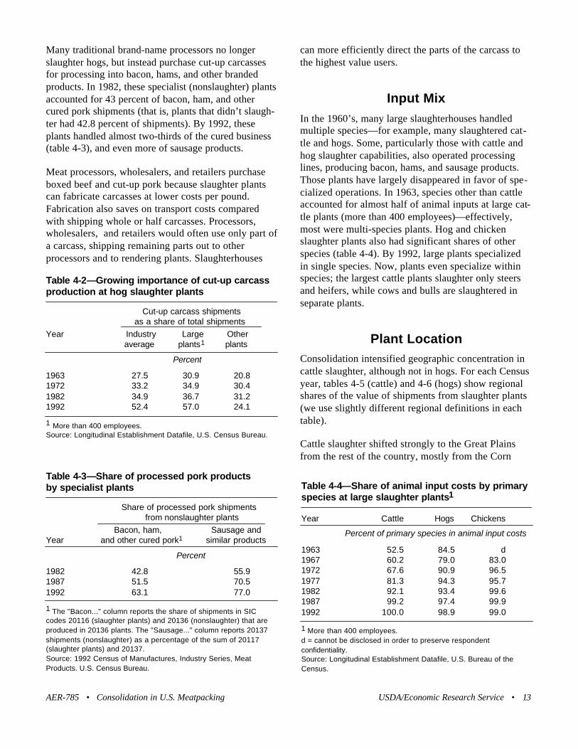
Many traditional brand-name processors no longerslaughter hogs, but instead purchase cut-up carcassesfor processing into bacon, hams, and other brandedproducts. In 1982, these specialist (nonslaughter) plantsaccounted for 43 percent of bacon, ham, and othercured pork shipments (that is, plants that didn’t slaugh-ter had 42.8 percent of shipments). By 1992, theseplants handled almost two-thirds of the cured business(table 4-3), and even more of sausage products.

Meat processors, wholesalers, and retailers purchaseboxed beef and cut-up pork because slaughter plantscan fabricate carcasses at lower costs per pound.Fabrication also saves on transport costs comparedwith shipping whole or half carcasses. Processors,wholesalers, and retailers would often use only part ofa carcass, shipping remaining parts out to otherprocessors and to rendering plants. Slaughterhouses

can more efficiently direct the parts of the carcass tothe highest value users.

Input MixIn the 1960’s, many large slaughterhouses handledmultiple species—for example, many slaughtered cat-tle and hogs. Some, particularly those with cattle andhog slaughter capabilities, also operated processinglines, producing bacon, hams, and sausage products.Those plants have largely disappeared in favor of spe-cialized operations. In 1963, species other than cattleaccounted for almost half of animal inputs at large cat-tle plants (more than 400 employees)—effectively,most were multi-species plants. Hog and chickenslaughter plants also had significant shares of otherspecies (table 4-4). By 1992, large plants specializedin single species. Now, plants even specialize withinspecies; the largest cattle plants slaughter only steersand heifers, while cows and bulls are slaughtered inseparate plants.

Plant LocationConsolidation intensified geographic concentration incattle slaughter, although not in hogs. For each Censusyear, tables 4-5 (cattle) and 4-6 (hogs) show regionalshares of the value of shipments from slaughter plants(we use slightly different regional definitions in eachtable).

Cattle slaughter shifted strongly to the Great Plainsfrom the rest of the country, mostly from the Corn


Table 4-2—Growing importance of cut-up carcassproduction at hog slaughter plants

Cut-up carcass shipments as a share of total shipments

Year Industry Large Other average plants1 plants

Percent

1963 27.5 30.9 20.81972 33.2 34.9 30.41982 34.9 36.7 31.21992 52.4 57.0 24.1

1 More than 400 employees.Source: Longitudinal Establishment Datafile, U.S. Census Bureau.

Table 4-3—Share of processed pork products by specialist plants

Share of processed pork shipmentsfrom nonslaughter plants

Bacon, ham, Sausage and Year and other cured pork1 similar products

Percent

1982 42.8 55.91987 51.5 70.51992 63.1 77.0

1 The "Bacon..." column reports the share of shipments in SICcodes 20116 (slaughter plants) and 20136 (nonslaughter) that areproduced in 20136 plants. The "Sausage..." column reports 20137shipments (nonslaughter) as a percentage of the sum of 20117(slaughter plants) and 20137.Source: 1992 Census of Manufactures, Industry Series, MeatProducts. U.S. Census Bureau.

Table 4-4—Share of animal input costs by primaryspecies at large slaughter plants1

Year Cattle Hogs Chickens

Percent of primary species in animal input costs

1963 52.5 84.5 d1967 60.2 79.0 83.01972 67.6 90.9 96.51977 81.3 94.3 95.71982 92.1 93.4 99.61987 99.2 97.4 99.91992 100.0 98.9 99.0

1 More than 400 employees.d = cannot be disclosed in order to preserve respondent confidentiality.Source: Longitudinal Establishment Datafile, U.S. Bureau of theCensus.

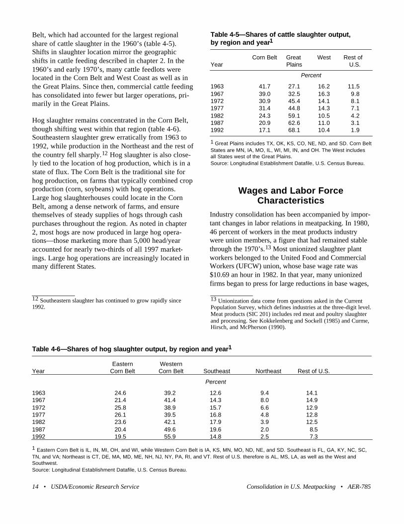
Belt, which had accounted for the largest regionalshare of cattle slaughter in the 1960’s (table 4-5).Shifts in slaughter location mirror the geographicshifts in cattle feeding described in chapter 2. In the1960’s and early 1970’s, many cattle feedlots werelocated in the Corn Belt and West Coast as well as inthe Great Plains. Since then, commercial cattle feedinghas consolidated into fewer but larger operations, pri-marily in the Great Plains.

Hog slaughter remains concentrated in the Corn Belt,though shifting west within that region (table 4-6).Southeastern slaughter grew erratically from 1963 to1992, while production in the Northeast and the rest ofthe country fell sharply.12 Hog slaughter is also close-ly tied to the location of hog production, which is in astate of flux. The Corn Belt is the traditional site forhog production, on farms that typically combined cropproduction (corn, soybeans) with hog operations.Large hog slaughterhouses could locate in the CornBelt, among a dense network of farms, and ensurethemselves of steady supplies of hogs through cashpurchases throughout the region. As noted in chapter2, most hogs are now produced in large hog opera-tions—those marketing more than 5,000 head/yearaccounted for nearly two-thirds of all 1997 market-ings. Large hog operations are increasingly located inmany different States.

Wages and Labor ForceCharacteristics

Industry consolidation has been accompanied by impor-tant changes in labor relations in meatpacking. In 1980,46 percent of workers in the meat products industrywere union members, a figure that had remained stablethrough the 1970’s.13 Most unionized slaughter plantworkers belonged to the United Food and CommercialWorkers (UFCW) union, whose base wage rate was$10.69 an hour in 1982. In that year, many unionizedfirms began to press for large reductions in base wages,


Table 4-5—Shares of cattle slaughter output, by region and year1

Corn Belt Great West Rest ofYear Plains U.S.

Percent

1963 41.7 27.1 16.2 11.51967 39.0 32.5 16.3 9.81972 30.9 45.4 14.1 8.11977 31.4 44.8 14.3 7.11982 24.3 59.1 10.5 4.21987 20.9 62.6 11.0 3.11992 17.1 68.1 10.4 1.9

1 Great Plains includes TX, OK, KS, CO, NE, ND, and SD. Corn BeltStates are MN, IA, MO, IL, WI, MI, IN, and OH. The West includesall States west of the Great Plains.Source: Longitudinal Establishment Datafile, U.S. Census Bureau.

Table 4-6—Shares of hog slaughter output, by region and year1

Eastern WesternYear Corn Belt Corn Belt Southeast Northeast Rest of U.S.

Percent

1963 24.6 39.2 12.6 9.4 14.11967 21.4 41.4 14.3 8.0 14.91972 25.8 38.9 15.7 6.6 12.91977 26.1 39.5 16.8 4.8 12.81982 23.6 42.1 17.9 3.9 12.51987 20.4 49.6 19.6 2.0 8.51992 19.5 55.9 14.8 2.5 7.3

1 Eastern Corn Belt is IL, IN, MI, OH, and WI, while Western Corn Belt is IA, KS, MN, MO, ND, NE, and SD. Southeast is FL, GA, KY, NC, SC,TN, and VA; Northeast is CT, DE, MA, MD, ME, NH, NJ, NY, PA, RI, and VT. Rest of U.S. therefore is AL, MS, LA, as well as the West andSouthwest. Source: Longitudinal Establishment Datafile, U.S. Census Bureau.

13 Unionization data come from questions asked in the CurrentPopulation Survey, which defines industries at the three-digit level.Meat products (SIC 201) includes red meat and poultry slaughterand processing. See Kokkelenberg and Sockell (1985) and Curme,Hirsch, and McPherson (1990).

12 Southeastern slaughter has continued to grow rapidly since1992.

to $8.25 an hour, consistent with what was beingoffered in non-union plants. The union at first accededto wage cuts, but by 1984 adopted a strategy to vigor-ously contest them, in the view that large wage cuts atolder unionized plants only postponed plant closings.Between 1983 and 1986, there were 158 work stop-pages in cattle and hog slaughter plants, involving40,000 workers. There were lengthy strikes, plant clos-ings, and deunionizations at some ongoing andreopened plants.14 By 1987, union membership hadfallen to 21 percent of the workforce, and has remainedat that lower level through the most recent data (1997);wage reductions were imposed in most plants, andwages have risen only modestly since then.

Declining unionization coincided with changes inslaughter plant demographics. Immigrants, primarilyfrom Southeast Asia, Mexico, and Central America,make up large and growing shares of the workforces atboth hog and cattle slaughter plants. This has led tostriking transformations in the rural communities thatmust provide schooling and social services to theworkers and their families (U.S. General AccountingOffice, 1998).

Most plant workers today perform routinized tasks ineither the slaughter or the fabrication department.Meatpacking work is hard and often hazardous; theuse of knives, hooks, and saws in noisy surroundingson slippery surfaces presents the risk of cuts, lacera-tions, and slips. The nature of the work also creates therisk of repetitive stress injuries, and the plant environ-ment can lead to pathogen-related illnesses. As aresult, meatpacking has had the highest rate of occupa-tional illnesses and injuries of all U.S. industries.During the late 1980’s, on-the-job injury and illnessrates in meatpacking rose sharply to a peak in 1991 of45.5 for every 100 workers. Since then, worker safetystatistics have improved, and the most recent Bureauof Labor Statistics data report that 30 out of every 100employees were injured or sickened on the job in1996.15

Perhaps because of the job hazards and workforcedemographics, labor turnover in meatpacking is quite

high, and in some establishments can reach 100 per-cent in a year as workers move to other employers orreturn to their native countries. The frequent move-ment of immigrant workers among plants and commu-nities limits union opportunities to organize, but alsoreflects immigration problems—district officials of theImmigration and Naturalization Service estimate thatas many as 25 percent of the workers at meatpackingplants in Iowa and Nebraska were illegal aliens (U.S.General Accounting Office, 1998).

Declines in unionization and increases in the use ofimmigrant workers coincided with sharp declines inreal wages (table 4-7). In 1977, mean wages rosesteadily with plant size in cattle and hog slaughterplants (SIC 2011), a pattern typical for manufacturing(Brown, Hamilton, and Medoff, 1990). The largest(1,000 or more employees) plants’ average hourlywages were 23 percent above the industry average, 30to 45 percent above wages at small (less than 500employees) plants, and more than double the wages ofworkers in poultry slaughter plants. Five years later,plants with 1,000 or more workers paid average wagesof $10 an hour, still 10 percent above the industryaverage, 20 to 40 percent above small plant wages,and almost twice the average wage in poultry plants.But by 1992, wages in large cattle and hog plants hadfallen sharply in nominal terms and dramatically inreal terms.16 Moreover, the plant size differential haddisappeared; the largest plants paid wages no differentfrom those offered in any of the plants with 100 ormore employees, and wages were only 17 percenthigher than those earned in poultry slaughter plants.


14 This summary draws on several articles appearing in theMonthly Labor Review, a publication of the Bureau of LaborStatistics of the U.S. Department of Labor.

15 The injury data refer to SIC 2011, all red meat slaughter plants.

16 The Consumer Price Index (CPI) increased by 131 percentbetween 1972 and 1982, and by another 45 percent between 1982and 1992. In 1992 dollars, large plant wages would have been$17.89 an hour in 1972, and the real 1972-1992 decline wouldamount to over 50 percent, with most of that concentrated in 1982-92. The CPI is widely considered to overstate inflation; if that’strue, then our adjustment overstates the size of the real wagedecline, although it does not affect comparisons across plants orslaughter classes within a year. If we accept the BoskinCommission’s estimate of CPI overstatement—1.1 percent peryear—then the 20-year decline in real wages at the largest cattleand hog plants would have been 40 percent.


Table 4-7—Average hourly wages in meatpacking, by year, industry, and plant size

Industry and plantsize (no. workers) 1967 1972 1977 1982 1987 1992

Dollars per hour1

SIC 2011 (Red meat):0-19 2.50 3.74 6.26 5.35 6.06 7.1720-99 2.70 3.71 5.69 6.88 7.79 8.23100-249 2.90 4.01 5.96 8.23 7.77 8.77250-499 3.29 4.36 6.33 9.43 8.40 8.46500-999 3.45 4.82 7.06 10.13 8.90 8.761,000 or more 4.04 5.33 8.44 10.00 8.50 8.65

Industry average 3.36 4.51 6.86 9.06 8.27 8.56

SIC 2015 (Poultry):0-19 1.92 2.50 3.37 5.00 5.78 6.8120-99 1.81 2.78 3.38 5.10 5.77 8.10100-249 1.76 2.42 3.52 5.23 6.33 7.16250-499 1.72 2.40 3.43 4.98 5.96 7.33500-999 1.79 2.35 3.48 5.14 6.17 7.391,000 or more n.a. n.a. 3.74 4.91 6.30 7.38

Industry average 1.76 2.40 3.48 5.06 6.16 7.37

1 Wages are production worker payroll divided by production worker hours.n.a. = not available.Source: Census of Manufactures, Industry Series , for relevant years.

Dramatically increased concentration in cattle slaughter(and increased concentration in hog slaughter) hascoincided with the ascendance of large plants in eachindustry. This suggests that new scale economies mayhave emerged and driven the increase in concentration.For scale economies to drive consolidation, they mustadhere through a range of plant sizes, and not simplyappear among very small plants. Moreover, for scaleeconomies to drive increases in concentration, techno-logical change should be scale-increasing—the largestplants should have cost advantages in the 1990’s thatare larger than those observed in the 1960’s and 1970’s.

Increased concentration in cattle and hog slaughteroccurred along with other developments. Cattle plantsmoved toward fabrication of carcasses into boxedbeef, while hog plants moved from extensive furtherprocessing (into hams, sausages, and the like) towardslaughter and simple fabrication. Since fabricationraises plant costs and alters input demands, cost analy-ses need to take account of product mix. More impor-tant, as larger plants often do more fabrication, anyanalysis of scale economies needs to take account ofproduct mix.

Finally, real wages fell from 1977 to 1992, while wagepremiums paid by large plants disappeared. We aim toestimate the effects of wage changes on costs, and soneed to separately identify the effects of changes in scaleeconomies and relative wages on large plant costs.

We need a statistical cost model that will allow us toestimate the extent of scale economies over a widerange of plant sizes, and that allows us to identifyscale-increasing technological change. The modelshould identify the effects of factor price changes oncosts, and should allow the effects of scale, factorprices, and product mix to change through time.

A Functional Form for Cost Estimation

For our purposes, we need to estimate a statistical costfunction that:

(1) estimates the effect of plant scale on costs, andallows the effect to vary with plant size;

(2) estimates the effects of product and input mix oncosts;

(3) identifies the effects of input prices on cost,allowing those effects to vary with plant size; and

(4) allows the above effects to vary over time as away to capture technological change.

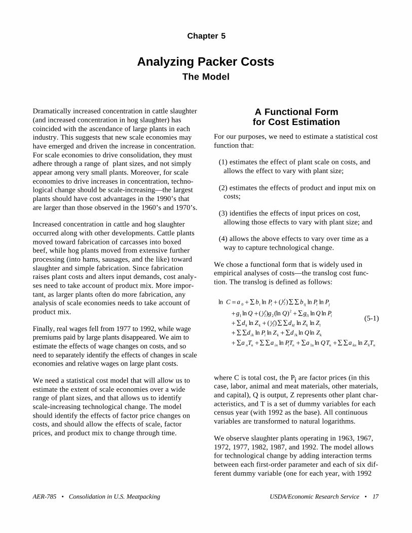
We chose a functional form that is widely used inempirical analyses of costs—the translog cost func-tion. The translog is defined as follows:

where C is total cost, the Pi are factor prices (in thiscase, labor, animal and meat materials, other materials,and capital), Q is output, Z represents other plant char-acteristics, and T is a set of dummy variables for eachcensus year (with 1992 as the base). All continuousvariables are transformed to natural logarithms.

We observe slaughter plants operating in 1963, 1967,1972, 1977, 1982, 1987, and 1992. The model allowsfor technological change by adding interaction termsbetween each first-order parameter and each of six dif-ferent dummy variable (one for each year, with 1992


Chapter 5

Analyzing Packer Costs The Model

nkknnniinnn

klkkiik

lkklkk

ili

jiijii

TZTQTPT

ZQZPZZZ

PQQQ

PPPC

lnlnln

lnlnlnlnlnln)(ln

lnln)(ln)(ln

lnln)(lnln

ln

21

222

11

21

0

αααα

δδδδ

γγγ

ββα

∑∑+∑+∑∑+∑+∑+∑∑+

∑∑+∑+∑+++

∑∑+∑+=

(5-1)

as the base). In the final form of the cost function, weused 4 factor prices, 3 Z variables, and 1 output vari-able, so that allowing for time-varying parametersadded 48 new parameters to the model.

The translog is a flexible functional form that allowsfor many possible production relationships, includingvarying returns to scale, nonhomothetic production(that is, optimal input ratios that vary with the level ofoutput), and nonconstant elasticities of input demand.One can estimate the cost function directly, but param-eter estimates are often inefficient because of multi-collinearity among the variables on the right-handside. Gains in efficiency can be realized by estimatingthe optimal, cost-minimizing input demand, or cost-share equations jointly with the cost function. Theequations are derived directly from the cost function asthe derivatives of total cost with respect to each inputprice, and share parameters with the cost function:

Because we follow standard practice and normalize allvariables (dividing them by their mean values beforeestimation), the first-order terms (the βi) can be inter-preted as the estimated cost share of input i at meanvalues of the right-hand variables; the other coeffi-cients capture changes in the estimated factor shareover time, and as factor prices, output, and plant char-acteristics move away from their mean values.

Some restrictions can be imposed on the estimatingequations in order to gain further improvements inefficiency (Berndt, 1991). For the cost function to behomogeneous of degree one in prices, the followingrestrictions must hold:

The restrictions reduce the number of parameters thatmust be estimated, since they imply that some parame-ters can be derived from combinations of others.Similarly, symmetry is also imposed on the model;under symmetry, the coefficients on all interactionterms with identical components are equal (that is, thecoefficients βij = βji, and δkl = δlk, for all i,j and allk,l).

We estimate the longrun cost function jointly in a mul-tivariate regression system with the four share equa-tions. Since factor shares sum to one, we dropped thecapital share equation to avoid a singular covariancematrix. Each equation could be estimated separatelyby ordinary least squares, but in order to take accountof likely cross-equation correlation in the error terms,we follow standard practice by using a nonlinear iter-ative seemingly unrelated regression procedure.

Measuring OutputModern slaughter plants produce many products. OurCensus data for cattle slaughter plants define severalproduct categories, including carcasses, hides, boxedbeef, ground beef, and byproducts. Each category isitself an aggregate—carcasses may be whole or inhalves or quarters, and boxed beef may come in a vari-ety of different cuts.

Multiple outputs create challenges for cost analysis.Suppose two plants slaughter the same number of cat-tle, but one operates a fabrication line while the otherproduces only carcasses. They will produce the samephysical quantity of output, and so a single productcost function will give them the same output level. Butthe fabrication plant will hire more workers, carry alarger investment in structures and equipment, and usemore energy and materials than the carcass-only plant;it will have higher costs because it will be performingmore processing of the carcass. The failure to accountfor product mix will, in this case, leave some variationin costs unaccounted for. But suppose that the plantthat fabricates is also larger, in that it handles morecattle—typical for the modern slaughter industry. Thenwe may observe higher costs per steer at the largerplant—that is, apparent diseconomies of scale, drivenby a failure to account for the different mix of prod-ucts at the larger plant.

To include multiple products in the cost function, wecould simply convert Q in the cost function to a vec-tor, with pounds of each output represented separatelyin the vector.17 But since many plants in the data setproduce zero amounts of some outputs, and logs are


17 See Morrison (1998) for an approach along these lines. Herdata included more precisely defined outputs for a more limited setof plants, as well as a different functional form for cost estimation,and so was better suited to that method.

ninkik

lijiji

iii

TZ

QPCXPPC

.ln

lnln/)()ln/()ln(

αδ

γββ

∑+∑

++∑+==∂∂

(5-2)

0,0 =∑=∑=∑=∑=∑ inikliiji αδγββ (5-3)

undefined at zero, the translog functional form cannotdirectly be adapted to the multiproduct approach.

Instead, we followed an approach that is commonlyused in the extensive literature on the estimation ofcost functions for transportation firms (railroads,trucking, airlines, shipping). In that literature, analystsoften have simple measures of output, defined in termsof ton-miles (for freight) and passenger-miles (exam-ples include Allen and Liu, 1995, for trucking; Baltagi,Griffin, and Rich, 1995, for airlines; Caves, et al.,1985, for railroads). But the simple measure can beproduced in a variety of ways; for example, costincurred in producing the same simple output can varyif the transport network routes to many different loca-tions (as opposed to a operating a few through-routes)or if the output is produced in many small deliveries(as opposed to a smaller number of large shipments).Transport cost functions often include measures ofroute and output characteristics in the cost function, inorder to capture the effect of network characteristicson costs.

We define a single output, pounds of meat produced,but we then add output characteristics to the equation(this is where the Z vector comes from). Our finalequation includes a measure of product mix. For cattle,this is defined as one minus the share of carcass ship-ments in the value of a plant’s output. The measure isalways defined in the translog, because carcass ship-ments are never 100 percent of output (byproducts arealways positive). Hide and byproduct shipments arenearly constant shares of total output, because they areproduced in close to fixed proportions to the numberof cattle slaughtered. As a result, the measure variesprimarily in proportion to the share of boxed beef in aplant’s output; increases in boxed beef mean declinesin the share of carcass output. As the cattle productmix variable increases, we ought to see increases intotal cost.

Our measure of product mix for hogs was one minusthe share of processed products (sausage, hams, etc.)in output. This measure will again always be definedin the translog, as processed product never takes up allof output. This is an inverse measure of processing,and costs should fall as the measure increases.

Each of these choices represents the best fitting option,after some experimentation. We tried several differentmeasures of product characteristics (such as one minusboxed beef). We also tried a multiple-product cost

function, with separate entries for pounds of carcassand pounds of boxed beef (setting zero values to lowbut positive values). But that form did not provide asstrong a fit as our preferred alternative, and we pre-ferred not to insert arbitrary values into our model.Finally, we also tried a measure based on the relativevalue of output, with those plants obtaining a highervalue of shipments per pound of output in any yearassumed to have a more complex product mix. Allproduct mix and multiple-product measures gave simi-lar qualitative results, but our final choice provided abetter fit to the data and a more direct interpretation.

Our final estimating equation includes two other vari-ables in the Z vector, a measure of input mix and adummy variable for single-plant firms. The measure ofinput mix is the share of live animals (primarily cattleand hogs) in combined live animal and purchased meatinput costs. Some slaughter plants purchase carcassesand other meats from other slaughter plants to supple-ment their own slaughtered carcasses as inputs to fab-rication lines. Plants with significant amounts of pur-chased meat may have different cost structures thanplants that purchase no meats, because those plantswill do proportionately more fabrication and lessslaughter.

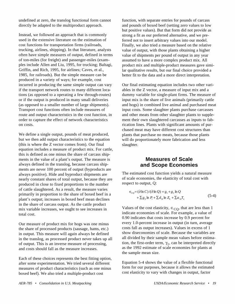
Measures of Scale and Scope Economies

The estimated cost function yields a natural measureof scale economies, the elasticity of total cost withrespect to output, Q:

Values of the cost elasticity, ∈CQ, that are less than 1indicate economies of scale. For example, a value of0.90 indicates that costs increase by 0.9 percent forevery 1.0-percent increase in output (in turn, averagecosts fall as output increases). Values in excess of 1show diseconomies of scale. Because the variables areall divided by their sample mean values before estima-tion, the first-order term, γ1, can be interpreted directlyas the 1992 estimate of scale economies for plants atthe sample mean size.

Equation 5-4 shows the value of a flexible functionalform for our purposes, because it allows the estimatedcost elasticity to vary with changes in output, factor


nklkili

CQ

TZP

QQC

ln

21

lnln

ln)ln/()ln(

αδγ

γγ

∑+∑+∑+

+=∂∂=∈(5-4)

prices, plant characteristics, and time. The parameterson the interaction terms between Q and years (the α1n)show how the mean cost elasticity changes throughtime, while the parameter on the the ln Q term (γ2)shows how the elasticity varies as we move away fromthe mean plant size to larger or smaller plant sizes.Finally, the other coefficients allow the estimateddegree of scale economies to vary with factor pricesand other plant characteristics.

We can also define a cost elasticity with respect tochanges in product mix. Define Zp as our measure ofproduct mix in cattle plants (one minus the share ofcarcasses). Then the product mix parameter is:

The first-order term in the cost elasticity, δp, providesa direct measure of the effect of increases in boxedbeef production on costs in 1992, given the physicalvolume of output, at sample means for all variables.The interaction terms on T (the time periods) showhow that elasticity changes as one moves back in time,while the coefficients on the Z interaction terms showhow the product mix elasticity varies as product mix,input mix, and ownership type vary. Finally, the coeffi-cient on physical output, δ1p, provides a direct esti-mate of scope economies. Positive values indicate thatexpanding product mix is more costly, per pound, inlarger plants than in small, while negative values indi-cate that expanding product mix is less costly in largerplants than in smaller plants.

Measures of Input Substitution and Demand

The translog functional form can be used to derivemeasures of substitution elasticities among inputs, aswell as measures of own-price and cross-price inputdemand elasticities. Some models assume a particularstructure of input demand in slaughter industries; forexample, “value-added” cost function models assumethat there is no substitution between animals and otherinputs in the production of meat. Our specificationallows us to test that assumption.

How is it possible to substitute other factors for ani-mals in the production of meat? Of course, at any oneplant, purchased carcasses can be substituted for ani-

mals in the fabrication process. But even without pur-chasing carcasses, yields—the amount of meat pro-duced from a carcass of a given size—do vary acrossanimals, plants, and time, and some of that variationmay be systematic, due to more intensive use of labor,machinery, and other materials. On the other hand,variation in yields does not necessarily imply that vari-ations in input prices were driving variations in inputsubstitution. That is an empirical issue, and translogparameter estimates allow us to test for the actual exis-tence of substitution, and to estimate its extent.

Substitution among labor, capital, and materials ismore likely, and the translog estimates will allow us toidentify the extent of substitution among those inputs,and to estimate price elasticities of input demand. Inturn, those estimates can be used as parameters inmodels that aim to simulate the response of the indus-try to changes in public policy or the industrial envi-ronment.

The Allen partial elasticities of input substitution forany inputs i and j, as derived from the translog func-tion, are equal to:

while price elasticities of input demand can be writtenas:

and

where the S’s are the factor shares of the ith and jthinputs, and γij is the coefficient on the jth input pricein the demand equation for the ith input (equation 5-2); it is also the coefficient on the interaction termbetween the ith and jth factor prices in the cost equa-tion (5-1). The coefficient γii is the coefficient on theith input’s price in the demand equation for that input,and is also the coefficient on the squared input priceterm in the cost function. Because, according to equa-tion 5-2, predicted factor shares will vary with output,time, factor prices, and plant characteristics, estimatesof equations 5-6 to 5-8 should use fitted shares at rep-resentative data values, and reported elasticities arealso representative values, which can vary with thedata.


npnipiip

kkpppCZp

TQP

ZZC

αδδ

δδ

∑++∑+

∑+=∂∂=∈

lnln

ln)ln/()ln( (5-5)

ijiijij SSS /)( +=∈ γ

),/()( jijiijij SSSS+= γσ

iiiiiij SSS /)( 2 −+=∈ γ

(5-6)

(5-7)

(5-8)

Data and Variable DefinitionsTable 5-1 provides definitions for the variables in thetranslog longrun cost functions estimated for cattle andfor hogs. All data are derived from the LRD files ofthe 1963-92 Census of Manufactures. Explanatoryvariables include input prices (labor, animals andmeat, other material, and capital) and plant output. Tothese standard explanatory variables, we add productmix, input mix, time shifts, and establishment typevariables.

Labor, meat, and other material input prices aredefined in a conventional fashion. Following Allenand Liu (1995), we define capital input costs as theopportunity cost of investing in plant and equipment.This definition of capital is imperfect because existingmachinery and building costs are reported at book

rather than real values. Additionally, capacity is ameasure of full capacity, and it is unlikely that allestablishments are producing at full capacity for allyears.

Product mix (PMIX) in cattle slaughter is defined asone minus the share of carcasses in total physical out-put; if the weight of hides and other byproducts can bethought of as varying in fixed proportions with totalplant slaughter, then this measure should vary largelywith variations in boxed beef production. The productmix variable in hog slaughter is one minus the quantityshare of processed products (such as hams andsausages). Increases in this measure reflect shifts toless complex processing, and should result in loweredcosts.


Table 5-1—Cost function variable definitions

Independent variables

PLAB Price of labor = (total plant labor costs) / (total employees).

PMEAT Price of meat inputs = (purchased animal costs + packed meat costs) / (pounds of live animal meatinputs + pounds of packed meat inputs).

PMAT Price of other material inputs = (energy costs+packing and packaging cost + other material costs) / (pounds live animal meat inputs + pounds packed meat inputs).

PCAP Price of capital = (OPPORTUNITY + NEW) / CAPACITY, where OPPORTUNITY = (machinery rentalprice) * (machinery book value) + (building rental price ) * (building book value); NEW is the cost of new machinery and buildings; CAPACITY is buildings and machinery book value. Note, machinery rental price is the industry-level cost per dollar of machinery expenditure; building rental price is industry-level cost per dollar of building expenditure.

Q Output of meat products, in thousands of pounds.

PMIX (cattle) Product mix: ( 1 - CARCASS%), where CARCASS% = (pounds of carcass shipments) / (total poundsof meat shipments).

PMIX(hogs) Product mix: (1 - SAUSAGE%), where SAUSAGE% = (pounds of sausage and ham products) / (total pounds of meat shipments).

IMIX (cattle) Input mix: ( 1 - CATTLE%), where CATTLE% = (pounds of live cattle meat inputs) / (total pounds of meat inputs).

IMIX (hogs) Input mix: (HOGS%), where HOGS% = (pounds of live hog meat inputs) / (total pounds of meat inputs).

ESTAB1 One for single-plant firms and zero otherwise. Shows shift for ownership type.

Dependent variables

COST Sum of labor, meat, materials, and capital input costs.

LABOR% (Salary and wages + supplemental labor costs) / COST.

MEAT% (Purchased animal costs + packed meat costs) / COST.

MAT% (Energy costs + packing and packaging cost + other material costs) / COST.

CAPITAL% (OPPORTUNITY + NEW) / COST. See PCAP above for definitions.

Input mix measures (IMIX) also vary between cattleand hog models. In cattle, the measure is one minusthe quantity share (in pounds) of cattle in total animaland meat inputs; that measure will move closer to oneas the plant purchases more carcasses from otherplants, or as it slaughters other species in addition tocattle. In hogs, the measure is simply the quantityshare of hogs in animal and meat inputs, and willmove closer to one as the plant specializes more inhog slaughter and purchases fewer carcasses.

Comparison to Other EconometricModels of Slaughter Industries

Our model differs in important respects from fourother extant estimations of slaughter cost functions forcattle and hogs. In chronological order, the four areBall and Chambers (1982), whose model covered themeat products sector for 1954-76; Melton andHuffman (1995), who analyzed costs in cattle and hogslaughter (separately) over 1963-88; Kambhampaty etal. (1996), who estimated a shortrun variable costfunction using weekly data for 16 large cattle slaughterplants in 1992; and Morrison (1998), who used thesame data source as Kambhampaty et al., to estimate ashortrun variable cost function using monthly data for42 plants in 1992.

Four features combine to distinguish our study andallow us to investigate some issues that other studiescannot: (1) disaggregated plant-level data covering awide range of plant sizes; (2) annual observations onplants covering census years between 1963 and 1992;(3) physical measures of output and measures of prod-uct and input mix; and (4) a translog specification thatallows for technological change by allowing parametervalues to shift over census years.

Ball and Chambers (1982) and Melton and Huffman(1995) each use samples that consist of annual timeseries observations on industry aggregates—for Balland Chambers, the aggregate is all red meat slaughterand processing. As Ball and Chambers point out, it isquite difficult to disentangle economies of scale fromtechnological change in aggregated time series models.Indeed, each reports estimates of economies of scalethat jump very sharply from year to year.Kambhampaty et al. (1996) and Morrison (1998) usedata on a relatively small number of large plants,observed at frequent intervals within a year. That dataset is better suited to the analysis of pricing and capac-ity utilization than to economies of scale and techno-logical change.

We contend that changes in product and input mixhave been an important feature of technologicalchange in the industry. For example, differences inboxed beef output across plants or over time willaffect costs, and omission of a product mix measurewill strongly affect estimates of scale economies ifproduct mix is associated with plant size (as chapter 3strongly suggests). Of the studies mentioned above,only Morrison (1998) accounts for differences in prod-uct mix. Kambhampaty et al. rely on a single-productoutput measure (chilled carcass weight), although theplants in the study produce sharply varying productmixes.18 The two earlier studies do not control fortemporal changes in product mix; chapter 3 shows thatsuch changes were substantial in the periods understudy, and correlated with growth in plant sizes.


18 They do provide separate estimates for plants that specialize incarcass production and those with fabrication capability, but thisapproach limits the size of their already small sample of plants,and ignores the large differences in fabrication output among fabri-cation plants.

We use the cost model to analyze costs at cattleslaughter plants. The data cover Census cattle slaugh-ter plants reporting in the years 1963, 1967, 1972,1977, 1982, 1987, and 1992, and include a total of2,541 useable plant observations over the 7 censusyears.19 Our primary goals are to identify the extent ofscale economies in slaughter, to determine whetherscale became more important over time, and to esti-mate the effect of product mix on plant costs.

Model Selection

The translog is a general functional form that can bespecified in different ways to capture many potentialcost effects. Alternative specific forms can allow forchanges in cost relationships through time, for differ-ent ways in which inputs may be combined, or for dif-ferent ways in which input and output mix can affectcosts. We were not certain of the best form prior toestimation. Model selection tests help to choose thebest fitting model among specific functional forms.

Tables 6-1 and 6-2 summarize the set of specific mod-els, and the results of the Gallant-Jorgenson (G-J) testsused to distinguish among them. We began with themost restrictive (I), a translog cost function with fourfactor prices (labor, capital, animal, and materialinputs) and the physical volume of output, but with nomeasures for input or output mix and no time shifters.It is restrictive in the sense that it imposes the assump-tions that input and output mix have no effect on costsand that coefficients do not change through time (notechnological change).

Model II adds input and product mix measures but nottime shifters; model I is decisively rejected in favor ofmodel II (table 6-2)—input and product mix measuresprovide statistically significant improvements in fit.Model III adds time shifters to model II; each first-

order coefficient is allowed to take on different valuesin different census years. Model III adds 42 newparameters to be estimated (6 new years times 7 vari-ables); G-J tests again favor the less restrictive model(III) over model II.

Model IV adds a dummy variable for single-establish-ment firms, and yields a statistically significant(though small) improvement in fit over model III.Models IVa and IVb impose new restrictions on modelIV. Model IVa drops variables involving input mix, butthat model is rejected; input mix variables, while indi-vidually not significant, together provide a statisticallysignificant improvement in fit. Finally, model IVbimposes homotheticity, by eliminating the interactionterms between factor prices and output volume (forc-ing factor shares to be invariant with respect to out-put). J-G tests reject homotheticity, and Model IVb, infavor of model IV. The best fitting model (IV) showsthe importance of input and product mix, and techno-logical change in determining cattle slaughter costs.

Summary of the Best Model

Because of the large number of estimated coefficientsin model IV, we have organized them into two tables.Table 6-3 reports first-order coefficients for 1992 andchanges in those coefficients in earlier years comparedwith 1992. Because all variables were standardized ontheir means before estimation, first-order coefficientscan be read directly as estimated elasticities at thesample mean. Table 6-4 repeats the 1992 first-ordercoefficients and coefficients for the quadratic andinteraction terms, showing how estimated elasticitiesvary as one moves away from sample means.

Consider factor price effects. First-order coefficients intable 6-3 can be interpreted as factor shares at samplemean data values. Animal and meat inputs (in thissample, almost all animal) account for over 83 percentof plant costs in 1992, while labor (PLAB) and othermaterials (PMAT—primarily packaging) are each lessthan 10 percent. The animal input share fell over time,


Chapter 6

Cattle Slaughter Cost Estimation

19 As is common with analyses of Longitudinal Research Data(LRD) files, we deleted observations on very small plants that didnot report all data, and some other observations with clear report-ing errors.

from just over 86 percent in 1977, while capital’s(PCAP) grew substantially from a small base. Laborand material shares showed hardly any change.

Because factor shares must sum to one, we left capitalout of the estimating equation, and recovered its valueas 1 minus the sum of the other three factors. Usingthat approach, capital’s share (PCAP) is less than 1percent in 1963 and over 3 percent in 1992.20

Estimated capital shares are consistent with Melton

and Huffman (1995), who find a mean 1963-88 capitalshare of 15.6 percent of beef value added, whichwould equate to a 2.65-percent share of total costs(assuming our mean estimate that cattle purchase costswere 83 percent of total costs).

Many interactions on factor prices (table 6-4) are high-ly significant, and the coefficients can be used to makeinferences about substitution among inputs (table 6-5).In particular, the own-price elasticity of demand foranimal and meat inputs, 0.0001, is about as close tozero as one can get in these measures. Given meat out-put, demand for animal and meat inputs does notchange at all as animal prices change. In short, one canfeasibly estimate “value added” cost functions on theassumption of separability between animals and otherinputs: that is, animal input demand is unresponsive tochanges in other factor prices.

The labor demand elasticity is estimated to be -0.294in 1992, close to the estimate (-0.373) reported byMelton and Huffman (1995) for the mean of their1963-88 data based on aggregate time series. It is alsoclose to the estimated elasticity of demand for othermaterials (-0.274), while that for capital is substantial-ly larger (-1.028). Capital and labor appear to be sub-stitutes in production, while substitution and cross-price elasticities between other input pairs is quite low.Table 6-5 also reports factor shares used in the estima-tion of 1992 elasticities. They are calculated at mean1992 sample values for other variables, and are there-fore different from factor shares in table 6-3, whichare calculated at mean sample-wide values for othervariables.

The factor share distribution identified here is a dis-tinctive feature of slaughter industries. Rarely does amaterial input (in this case, cattle) account for such alarge share of costs. The large share accorded to cattleinputs suggests that there are some important limits tothe effect of slaughter scale economies on costs. Theprocesses that drive scale economies are limited to thecooperating inputs of labor, capital, and other materi-als, which together make up only a fifth to a tenth oftotal slaughter costs.21


Table 6-1—Cattle slaughter cost function models,by goodness of fit

Model Description G-J Parameters statistic estimated

I Translog, factor prices and output only 8324 15

II Adds product and input mix to I 8252 28

III Adds first order time shifts to II 7827 70

IV Adds single-establishment dummy to III 7799 77

IVa Drops input mix variables from IV 7855 58

IVb Imposes homotheticity on IV 7820 74

Source: Authors' estimates, based on models and data described intext.

Table 6-2—Tests of model selection, cattle slaughter cost function

Test statistics1

Critical Chi-Comparison d.f. value@ 99 square

II vs. I 13 27.69 72III vs. II 42 66.18 425IV vs. III 7 18.48 28IV vs. IVA 19 36.19 56IV vs. IVB 3 11.34 21

1 Chi-square statistics are the difference in G-J statistics in modelsreported in table 6-1. Degrees of freedom (d.f) are the differences inthe number of estimated parameters.


20 The skewed distribution of factor shares gives rise to some vio-lations of monotonicity conditions. Specifically, predicted factorshares for capital are negative in 9 percent of observations, and“other materials” factor shares are negative for 12 percent ofobservations. The violations occur primarily among the smallestplants, and early in the period.

21 Potential scale economies in slaughter plants arise from oppor-tunities to achieve specialization of labor, and from opportunitiesto apply capital equipment in larger plants. But even if thesestrategies result in substantial reductions in slaughter and fabrica-tion costs, those costs are small fractions of total plant costs,swamped by animal purchase costs.

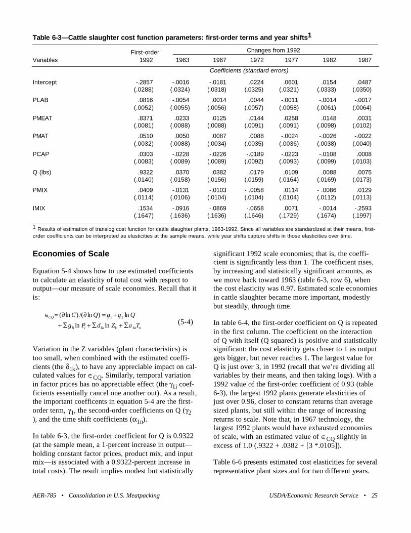
Economies of Scale

Equation 5-4 shows how to use estimated coefficientsto calculate an elasticity of total cost with respect tooutput—our measure of scale economies. Recall that itis:

Variation in the Z variables (plant characteristics) istoo small, when combined with the estimated coeffi-cients (the δ1k), to have any appreciable impact on cal-culated values for ∈CQ. Similarly, temporal variationin factor prices has no appreciable effect (the γ1i coef-ficients essentially cancel one another out). As a result,the important coefficents in equation 5-4 are the first-order term, γ1, the second-order coefficients on Q (γ2), and the time shift coefficients (α1n).

In table 6-3, the first-order coefficient for Q is 0.9322(at the sample mean, a 1-percent increase in output—holding constant factor prices, product mix, and inputmix—is associated with a 0.9322-percent increase intotal costs). The result implies modest but statistically

significant 1992 scale economies; that is, the coeffi-cient is significantly less than 1. The coefficient rises,by increasing and statistically significant amounts, aswe move back toward 1963 (table 6-3, row 6), whenthe cost elasticity was 0.97. Estimated scale economiesin cattle slaughter became more important, modestlybut steadily, through time.

In table 6-4, the first-order coefficient on Q is repeatedin the first column. The coefficient on the interactionof Q with itself (Q squared) is positive and statisticallysignificant: the cost elasticity gets closer to 1 as outputgets bigger, but never reaches 1. The largest value forQ is just over 3, in 1992 (recall that we’re dividing allvariables by their means, and then taking logs). With a1992 value of the first-order coefficient of 0.93 (table6-3), the largest 1992 plants generate elasticities ofjust over 0.96, closer to constant returns than averagesized plants, but still within the range of increasingreturns to scale. Note that, in 1967 technology, thelargest 1992 plants would have exhausted economiesof scale, with an estimated value of ∈CQ slightly inexcess of 1.0 (.9322 + .0382 + [3 *.0105]).

Table 6-6 presents estimated cost elasticities for severalrepresentative plant sizes and for two different years.


Table 6-3—Cattle slaughter cost function parameters: first-order terms and year shifts1

First-order Changes from 1992

Variables 1992 1963 1967 1972 1977 1982 1987

Coefficients (standard errors)

Intercept -.2857 -.0016 -.0181 .0224 .0601 .0154 .0487(.0288) (.0324) (.0318) (.0325) (.0321) (.0333) (.0350)

PLAB .0816 -.0054 .0014 .0044 -.0011 -.0014 -.0017(.0052) (.0055) (.0056) (.0057) (.0058) (.0061) (.0064)

PMEAT .8371 .0233 .0125 .0144 .0258 .0148 .0031(.0081) (.0088) (.0088) (.0091) (.0091) (.0098) (.0102)

PMAT .0510 .0050 .0087 .0088 -.0024 -.0026 -.0022(.0032) (.0088) (.0034) (.0035) (.0036) (.0038) (.0040)

PCAP .0303 -.0228 -.0226 -.0189 -.0223 -.0108 .0008(.0083) (.0089) (.0089) (.0092) (.0093) (.0099) (.0103)

Q (lbs) .9322 .0370 .0382 .0179 .0109 .0088 .0075(.0140) (.0158) (.0156) (.0159) (.0164) (.0169) (.0173)

PMIX .0409 -.0131 -.0103 - .0058 .0114 - .0086 .0129(.0114) (.0106) (.0104) (.0104) (.0104) (.0112) (.0113)

IMIX .1534 -.0916 -.0869 -.0658 .0071 -.0014 -.2593(.1647) (.1636) (.1636) (.1646) (.1729) (.1674) (.1997)

1 Results of estimation of translog cost function for cattle slaughter plants, 1963-1992. Since all variables are standardized at their means, first-order coefficients can be interpreted as elasticities at the sample means, while year shifts capture shifts in those elasticities over time.

nklkili

CQ

TZP

QQC

ln

21

lnln

ln)ln/()ln(

αδγ

γγ

∑+∑+∑+

+=∂∂=∈(5-4)

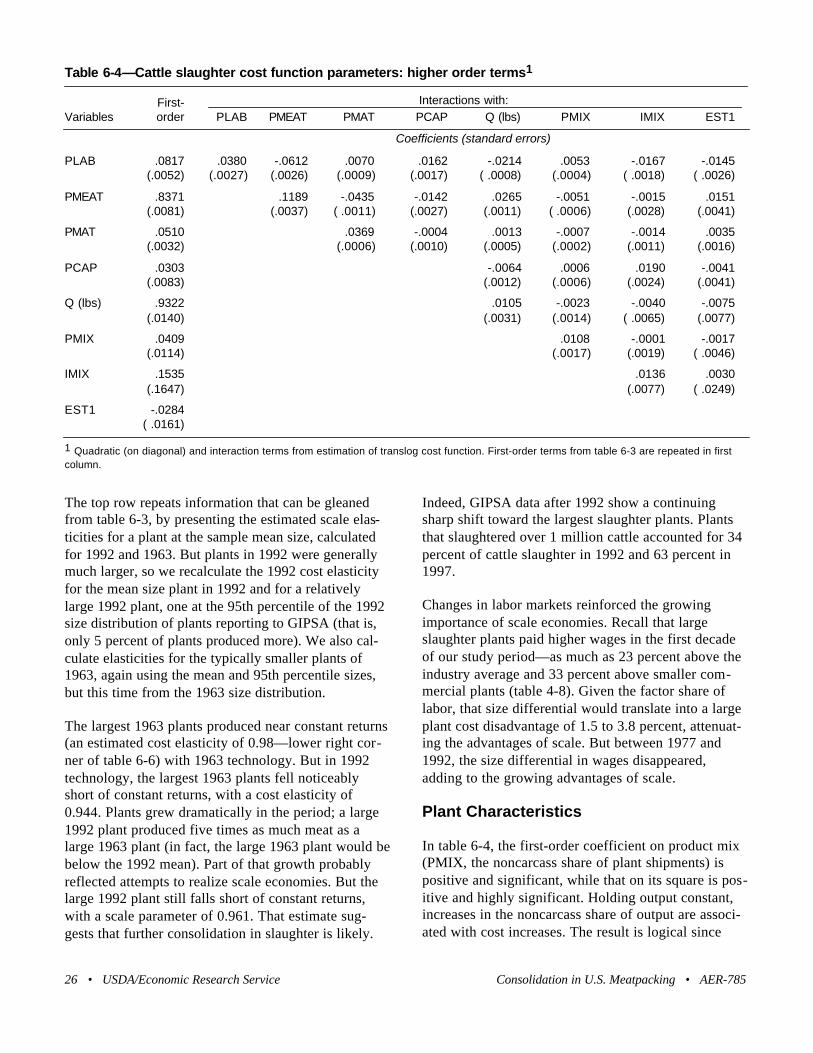
The top row repeats information that can be gleanedfrom table 6-3, by presenting the estimated scale elas-ticities for a plant at the sample mean size, calculatedfor 1992 and 1963. But plants in 1992 were generallymuch larger, so we recalculate the 1992 cost elasticityfor the mean size plant in 1992 and for a relativelylarge 1992 plant, one at the 95th percentile of the 1992size distribution of plants reporting to GIPSA (that is,only 5 percent of plants produced more). We also cal-culate elasticities for the typically smaller plants of1963, again using the mean and 95th percentile sizes,but this time from the 1963 size distribution.

The largest 1963 plants produced near constant returns(an estimated cost elasticity of 0.98—lower right cor-ner of table 6-6) with 1963 technology. But in 1992technology, the largest 1963 plants fell noticeablyshort of constant returns, with a cost elasticity of0.944. Plants grew dramatically in the period; a large1992 plant produced five times as much meat as alarge 1963 plant (in fact, the large 1963 plant would bebelow the 1992 mean). Part of that growth probablyreflected attempts to realize scale economies. But thelarge 1992 plant still falls short of constant returns,with a scale parameter of 0.961. That estimate sug-gests that further consolidation in slaughter is likely.

Indeed, GIPSA data after 1992 show a continuingsharp shift toward the largest slaughter plants. Plantsthat slaughtered over 1 million cattle accounted for 34percent of cattle slaughter in 1992 and 63 percent in1997.

Changes in labor markets reinforced the growingimportance of scale economies. Recall that largeslaughter plants paid higher wages in the first decadeof our study period—as much as 23 percent above theindustry average and 33 percent above smaller com-mercial plants (table 4-8). Given the factor share oflabor, that size differential would translate into a largeplant cost disadvantage of 1.5 to 3.8 percent, attenuat-ing the advantages of scale. But between 1977 and1992, the size differential in wages disappeared,adding to the growing advantages of scale.

Plant Characteristics

In table 6-4, the first-order coefficient on product mix(PMIX, the noncarcass share of plant shipments) ispositive and significant, while that on its square is pos-itive and highly significant. Holding output constant,increases in the noncarcass share of output are associ-ated with cost increases. The result is logical since


Table 6-4—Cattle slaughter cost function parameters: higher order terms1

First- Interactions with:Variables order PLAB PMEAT PMAT PCAP Q (lbs) PMIX IMIX EST1


PLAB .0817 .0380 -.0612 .0070 .0162 -.0214 .0053 -.0167 -.0145(.0052) (.0027) (.0026) (.0009) (.0017) ( .0008) (.0004) ( .0018) ( .0026)

PMEAT .8371 .1189 -.0435 -.0142 .0265 -.0051 -.0015 .0151(.0081) (.0037) ( .0011) (.0027) (.0011) ( .0006) (.0028) (.0041)

PMAT .0510 .0369 -.0004 .0013 -.0007 -.0014 .0035(.0032) (.0006) (.0010) (.0005) (.0002) (.0011) (.0016)

PCAP .0303 -.0064 .0006 .0190 -.0041(.0083) (.0012) (.0006) (.0024) (.0041)

Q (lbs) .9322 .0105 -.0023 -.0040 -.0075(.0140) (.0031) (.0014) ( .0065) (.0077)

PMIX .0409 .0108 -.0001 -.0017(.0114) (.0017) (.0019) ( .0046)

IMIX .1535 .0136 .0030(.1647) (.0077) ( .0249)

EST1 -.0284( .0161)

1 Quadratic (on diagonal) and interaction terms from estimation of translog cost function. First-order terms from table 6-3 are repeated in firstcolumn.

higher values of PMIX imply more fabrication, andtherefore more labor, capital, and materials.

For product mix (PMIX), the interaction terms withfactor prices are all highly significant (table 6-4, col-umn 7). As the noncarcass share gets larger, the shareof costs accounted for by labor gets larger while thataccounted for by animals gets smaller, also logicalgiven the value added in fabrication.

We can show the effects of likely changes in PMIX onaverage costs, with the approach taken above for scaleeconomies. Estimated average costs rise by about 3.2percent, for a large plant (at the 95th percentile of thesize distribution), as the plant goes from minimal toextensive fabrication (from PMIX of 0.38 to 0.90).22

Finally the negative and marginally significant sign onthe interaction of PMIX and output (Q) gives evidenceof scope economies—the scale parameter gets smaller(steeper, or further below 1) as PMIX gets larger. Butthe effect is small: a plant at the 75th percentile of the1992 size distribution (about a third as large as a plantat the 95th percentile) would incur additional fabrica-tion costs of 3.6 cents per pound in going from mini-mal to extensive fabrication, compared with 3.2 centsper pound for a plant at the 95th percentile.

Most of the individual coefficients involving input mix(IMIX, the share of animals in meat and animalinputs) are small and not significant, although the G-Jtests in table 6-2 favor retaining the measure. There

are three exceptions. The coefficient on IMIX squaredis small but positive and statistically significant, sug-gesting that costs increase as the animal share increas-es above its mean, given output. The coefficient on theinteraction term with the price of labor is negative,while that on capital is positive, with each highly sig-nificant. Labor shares are lower, and capital shares arehigher, in plants that use higher ratios of animal tomeat inputs.

Tables 6-3 and 6-4 also show that, all else equal, sin-gle-establishment firms have lower costs, as well asslightly different input shares (higher shares of animalsand materials, and lower labor shares). Interpretation isdifficult here—the coefficients could be picking updifferences in accounting techniques; differences inproduct mix, input mix, or scale that our model doesnot capture; or real efficiency differences. Becausethese results are hard to interpret, we look at single-establishment variables as control measures, and othercoefficients are not affected by their inclusion.

Finally, consider changes in the model’s intercept overtime, in table 6-3. None of the coefficients are signifi-cant, and they show no consistent sign pattern. Byimplication, there are no temporal changes in slaughtercosts that are not picked up by movements in factorprices, scale, and product mix effects. This suggeststhat much of the cattle slaughter industry’s productivi-ty growth is accounted for by scale economies, eitherthrough changes in the estimated scale parameter orthrough increases in plant size to take advantage ofscale economies.

What Do Other Studies Find?

Our findings for scale economies conflict with Balland Chambers (1982) and with Melton and Huffman


22 In turn, average processing costs (value added) would rise byslightly over 30 percent, if animal acquisition costs were 90 per-cent of the total at the minimal plant and were unchanged as onemoves to the extensive plant.

Table 6-5—Mean input shares and elasticities,19921

Input price variables

Item PLAB PMEAT PMAT PCAP

Input share .0587 .8622 .0550 .0301

∈ii -0.294 0.0001 -0.274 -1.028

σijPLAB -5.01 -0.209 3.167 10.170PMEAT 0.0001 0.083 0.453PMAT -4.98 0.789PCAP -34.10

1 All values are calculated using mean 1992 data values andparameters from tables 6-3 and 6-4. The own-price input demandelasticities (∈ii) are calculated holding output and other factors con-stant, while the elasticities of substitution (σij) are calculated usingAllen's formula.

Table 6-6—Estimated cost elasticity coefficients,by plant size and year1

Technology vintagePlant size 1992 1963

Sample mean 0.932 0.969

1992 mean 0.946 0.9831992 95th percentile 0.961 0.998

1963 mean 0.925 0.9621963 95th percentile 0.944 0.981

1 The coefficients report the percentage change in total costs corre-sponding to a 1-percent change in output, for plants of differingsizes and technological vintages.

(1995). Each reports cost elasticities that range sub-stantially above and below 1, with large economies ofscale in some years and diseconomies in others. Balland Chambers estimate a value-added cost functionusing annual data for the entire meat products sector(SIC 201). They report cost elasticities for the early1970’s, and find scale economies that are substantiallylarger than those reported here. Moreover, their esti-mates vary, as they report substantial diseconomies ofscale for 1971. Melton and Huffman estimate a value-added cost function using aggregated annual data forbeef and pork slaughter separately. They reporteconomies of scale for 1975, and very large disec-onomies of scale for the 1980’s.

Each study used highly aggregated data that affordedlimited opportunities to distinguish among capacityutilization, technological change, and the realization ofscale economies, and neither attempted to control forchanges in product and input mix over the period.Since large plants led the move to greater fabricationin beef (table 4-1), those plants would have begun toincur higher average costs per head than smallerslaughter-only plants, and analyses that fail to controlfor product mix would likely report evidence of disec-onomies.

Kambhampaty et al. (1996) and Morrison (1998) esti-mate shortrun variable cost functions, and those datasets are poorly suited to estimation of longrun scaleeconomies. Each finds important shortrun increasingreturns to scale, in that average costs decline as outputincreases at plants within the year. In that respect, theysupport the assertions of Ball and Chambers (1982)and Ward (1990)—that capacity utilization is animportant element in average costs at cattle slaughterplants.

Our findings on economies of scale are quite similar tothe estimates reported for the simulation models ofDuewer and Nelson (1991) and of Ward (1993), whoreports the work of his student, Sersland (1985). Thesimulation models differ from our econometric modelin one major respect: while our econometric estimatesare based on the statistical estimation of cost functionsusing operating data from many plants, simulationmodels rely on idealized operations across a few stan-dardized plant types. Sersland obtained her data from amail survey of managers, who provided her with costestimates for several specified plant types, whileDuewer and Nelson constructed an engineering-eco-nomic model of costs at specified plant types, bybuilding up from specified activities, input quantities,and input prices.

In table 6-7, we calculate indexes of average cost (perhead), based on the data in Ward and in Duewer andNelson, and compare them to calculations based on themodels and data underlying this report. We separatelyreport indexes for slaughter cost, which excludes pur-chase expenses for animals, and total cost, whichincludes animal expenses. All estimates were convert-ed to index numbers to preserve Census confidentiali-ty. Index numbers reveal no actual cost estimates, butshow how estimated average costs change as plant sizevaries.23


23 We can use our model to estimate costs per head for a hypo-thetical plant. We first estimate the 1992 animal share of total costsfor a large plant (1.1 million head annually, or 300 head per hourin a two-shift-per-day plant operated 40 hours per week). Then,using our census data for the mean 1992 animal factor price, wecalculate total cost per pound and subtract the animal cost fromthat to get slaughter/fabrication cost per pound. We then multiplyby the 1992 average meat yield (701 pounds) to estimate a cost perhead. The resulting estimate, $59 per head, compares with D&N’sestimate of $60 dollars per head at a similarly sized plant andSersland’s estimate of $55 (Ward, 1993). Our analysis is based on

Table 6-7—Comparing size-cost estimates in cattle slaughter

Cost/head, including cattle acquisition Cost/head, slaughter & fabrication only Head/year W&S1 D&N Census W&S D&N Census

Index

175,000 102.3 101.4 104.3 116.9 111.2 130.7300,000 101.2 100.6 101.5 109.3 104.3 110.7425,000 100.0 100.0 100.0 100.0 100.0 100.0850,000 98.7 98.4 97.9 90.4 87.1 85.01,100,000 97.7 98.0 97.3 82.6 84.4 80.71,350,000 97.5 98.0 97.0 81.3 84.4 78.6

1 "W&S" refers to estimates of Ward (1993), derived from Sersland; "D&N" refers to estimates derived from Duewer and Nelson (1991);"Census" refers to estimates derived from tables 6-3 and 6-4. In order to protect the confidentiality of Census data, the data are presented asindex numbers, with 425,000 set to 100.

We began with Ward, who derives a set of annualslaughter volumes from typical combinations of hourlyslaughter speeds and daily shifts (the three smallerplants are assumed to operate single shifts, with corre-spondingly smaller investments in storage capacity,while the three larger plants are designed to operatetwo daily shifts). Each simulated plant performsslaughter and fabrication functions. For each simulatedplant, we took Ward’s slaughter/fabrication cost esti-mates, and then converted them to index numbers withhis midpoint plant (425,000 head per year) set to100.24 To convert Ward’s slaughter cost indexes tototal cost indexes, we then made two assumptionsabout cattle prices: that cattle costs account for 86 per-cent of total costs at Ward’s midpoint plant (consistentwith the 1992 Census mean) and that all plants pay thesame cattle prices. With those assumptions, we canderive an estimated cattle price from Ward’s data, andthen simply add that price to average slaughter fabrica-tion costs to get average total costs.

Duewer and Nelson’s size categories do not match upexactly to Ward’s. For comparison, we interpolatedaverage costs between Duewer and Nelson’s outputlevels to get to costs for Ward’s output levels.25 Weadded in the estimated cattle price to get to total costs,and converted Duewer and Nelson’s estimates to indexnumbers, with average costs at an output of 425,000head set to the base of 100.

We next calculated a total cost index for our model,first converting our output measure (pounds of meat)to cattle numbers with the Census mean meat yield of701 pounds per animal. We estimated total and aver-age costs for a plant with output corresponding to425,000 head per year, and set its index to 100.Finally, we used our estimated cost function to project

how total and average costs would vary with output,holding other variables constant at 1992 means.

Average total costs fall with plant size in each model,but the declines are very modest (table 6-7). In partic-ular, as we move to the largest plant from the midpointplant, average total costs per head fall by 3.0 percentin the Census model, 2.5 percent in Ward, and 2.0 per-cent in Duewer and Nelson. Average total costs risemore sharply in the Census model as we move towardsmaller plants from the midpoint plant (a 4.3-percentrise vs. 2.3 percent in Ward and 1.4 percent in D&N),suggesting more severe diseconomies of small scale.26

Average costs for slaughter/fabrication alone fall byaround 20 percent from midpoint to largest plant(Census reports a 22.4-percent decline, compared with18.7 percent for W&S and 15.6 percent for D&N).This comparison also points up one area of differ-ence—the Census model reports continuing scaleeconomies among the very largest plants, while D&Nreport constant returns among the largest plants.

Given the uncertainties involved in comparing econo-metric and simulation models, the two approaches stilltell a common story regarding economies of scale incattle slaughter. There are large scale economies in theslaughter and fabrication functions, the economiesextend across a wide range of plant sizes, and theytranslate into modest but significant economies ofscale when considering total costs (including animalprocurement costs).

We can use table 6-7 to gauge the relative importanceof technological and pecuniary scale effects. The tableshows technological scale economies: given 1992 fac-tor prices, total costs per head fall by 2 to 3 percent aswe move from average sized to very large plants.Pecuniary diseconomies at larger 1970’s plants (in theform of higher wages) increased large plant costs by1.5 to 3.8 percent, compared with smaller plants.Pecuniary diseconomies were close in magnitude totechnological economies, and their disappearance in


1992 factor prices and technology, while D&N’s analysis is for1988 and Sersland’s for 1985. As noted above, our incrementalcost of adding fabrication lines in a plant appears to be low, com-pared with the simulation studies. Nevertheless, our estimatedcosts are quite close, and provide further confidence for the econo-metric estimates.

24 The largest plant listed in table 6-7 matches the largest plantsoperating today, while plants that slaughter more than a millionhead accounted for just over half of all steer and heifer slaughterin 1996 (table 3-3). Plants slaughtering less than a half millionaccounted for nearly two thirds of 1982 slaughter and less thanone fifth of 1996 slaughter.

25 We selected Duewer and Nelson’s estimates corresponding toslaughter/fabrication operations, 40-hour work weeks, single shiftsfor smaller plants, and double shifts for larger plants.

26 Capacity utilization may play a role here. Ward (1990) and1992 GIPSA data suggest that larger plants have systematicallyhigher levels of capacity utilization, which would show up as partof scale economies in our econometric cost functions. Our costestimates for Ward and D&N plants assume no differences incapacity utilization across plants. If we alternatively assume thatsmall plants operate 32 instead of 40 hours per week, then theD&N index at the smallest plant size rises to 102.9, closing halfthe gap with the Census indexes.


the 1980’s reinforced the effects of growing techno-logical scale economies in providing cost advantagesto large plants.

Conclusion

The estimated cost function finds small but importantscale economies. They became more importantthrough time, and extend throughout the range of plantsizes in the 1990’s, suggesting that the largest plantscontinue to have cost advantages over smaller com-mercial operations. Wage-based pecuniary disec-onomies limited the realization of technological scaleeconomies in the 1970’s, and their disappearance inthe 1980’s reinforced growing large-plant cost advan-tages. Changes in product mix, toward greater fabrica-tion, have small positive effects on costs, and addslightly less to unit costs in larger plants. The resultssuggest that slaughter plants shifted to greater fabrica-tion because they could do so at lower costs than car-cass buyers (meat wholesalers and retailers) could,and that larger plants had greater fabrication advan-tages than smaller plants.

We apply the models described in chapter 5 to theanalysis of costs at hog slaughter plants; the data coverCensus plants reporting in the years 1963, 1967, 1972,1977, 1982, 1987, and 1992, and include a total of1,142 plant observations over the 7 census years. Ourprimary goals are to identify the extent of scaleeconomies in slaughter, to determine whether scalebecame more important over time, and to estimate theeffect of product mix on plant costs.

Model Selection

We followed the same approach used in chapter 6 forthe estimation of cattle slaughter cost functions, apply-ing Gallant-Jorgenson tests to distinguish among dif-ferent functional forms. Table 7-1 provides descrip-tions of the tested models, while table 7-2 summarizesthe results of the G-J tests. The results mirrored thefindings for cattle slaughter in that the most generalmodel (IV) provided statistically significant improve-ments in fit over each of the more restrictive models.

As in the cattle models, the most restrictive model (I)contained four factor prices (labor, capital, animalinputs, and other materials) and the physical volume ofoutput, but no time shifters and no measures of outputor input mix. Model I was decisively rejected in favorof model II, which added measures of output and inputmix. Model II was then compared with model III,which represents technological change by allowing allfirst-order coefficients to vary over time. Model IIIadded 42 new estimated parameters to the cost func-tion, but that more flexible model provides animprovement in fit, at a 99-percent level of signifi-cance. Finally, model IV adds a dummy variable forsingle-establishment firms, and is favored over the lessflexible model III.

Table 7-2 also reports tests of two additional restric-tions on model IV. Model IVa drops the terms involv-ing input mix (that is, sets coefficients to zero), but therestrictions are strongly rejected—it is important toaccount for differences in the mix of animal and meatinputs. Model IVb imposes homotheticity, under which

factor proportions are invariant to levels of output. G-Jtests decisively reject homotheticity. The best model(IV) is nonhomogeneous and nonhomothetic; itincludes measures of product and input mix as well asa shift variable for single-establishment firms; and itallows all first-order coefficients to vary over time.

Summary of the Best Model

Table 7-3 reports all first-order coefficients for 1992and first-order time shifters for earlier years, whiletable 7-4 repeats the 1992 first-order coefficients andreports coefficients on the quadratic and interactionterms. In table 7-3, the first-order coefficients can beinterpreted as factor shares at the sample mean.Animal and meat inputs accounted for just under 73percent of hog slaughter costs in 1992 (recall that incattle slaughter this share was larger, 83 percent).Labor accounted for 11 percent of costs, while capitaland other materials each accounted for 8 percent in1992. The capital share rose sharply after the late1970’s, while all other factor shares fell. Table 7-4 alsoreports some important interactions of factor shareswith output.

The skewed distribution of factor shares carries thesame implications for hog as for cattle slaughter. First,as long as the prices paid for hogs are invariant toplant size, substantial scale economies in slaughter andfabrication will translate into small scale economiescalculated on total costs, because total costs will bedominated by hog purchase expenses. Second, wagechanges will lead to small product price changes,because wages form such a small share of total costs.Finally, wage changes that are not passed through asproduct price changes can lead to large changes inreturns on invested capital, since labor and capitaleach form small shares of total cost.

Table 7-5 reports price elasticities of input demandusing mean 1992 data values. All four inputs havedownward sloping demand curves—the estimatedelasticities are negative at the mean. The estimatedprice elasticity of demand for labor is close to that


Chapter 7

Hog Slaughter Cost Estimation

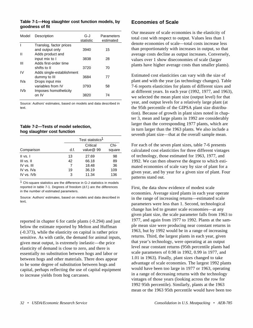
reported in chapter 6 for cattle plants (-0.294) and justbelow the estimate reported by Melton and Huffman (-0.373), while the elasticity on capital is rather pricesensitive. As with cattle, the demand for animal inputs,given meat output, is extremely inelastic—the priceelasticity of demand is close to zero, and there isessentially no substitution between hogs and labor orbetween hogs and other materials. There does appearto be some degree of substitution between hogs andcapital, perhaps reflecting the use of capital equipmentto increase yields from hog carcasses.

Economies of Scale

Our measure of scale economies is the elasticity oftotal cost with respect to output. Values less than 1denote economies of scale—total costs increase lessthan proportionately with increases in output, so thataverage costs decline as output increases. Conversely,values over 1 show diseconomies of scale (largerplants have higher average costs than smaller plants).

Estimated cost elasticities can vary with the size ofplant and with the year (as technology changes). Table7-6 reports elasticities for plants of different sizes andat different years. In each year (1992, 1977, and 1963),we selected the mean plant size (output level) for thatyear, and output levels for a relatively large plant (atthe 95th percentile of the GIPSA plant size distribu-tion). Because of growth in plant sizes noted in chap-ter 3, mean and large plants in 1992 are considerablylarger than the corresponding 1977 plants, which arein turn larger than the 1963 plants. We also include aseventh plant size—that at the overall sample mean.

For each of the seven plant sizes, table 7-6 presentscalculated cost elasticities for three different vintagesof technology, those estimated for 1963, 1977, and1992. We can then observe the degree to which esti-mated economies of scale vary by size of plant for agiven year, and by year for a given size of plant. Fourpatterns stand out.

First, the data show evidence of modest scaleeconomies. Average sized plants in each year operatein the range of increasing returns—estimated scaleparameters were less than 1. Second, technologicalchange has led to greater scale economies—at anygiven plant size, the scale parameter falls from 1963 to1977, and again from 1977 to 1992. Plants at the sam-ple mean size were producing near constant returns in1963, but by 1992 would be in a range of increasingreturns. Third, the largest plants in each year, giventhat year’s technology, were operating at an outputlevel near constant returns (95th percentile plants hadscale parameters of 0.98 in 1992, 0.99 in 1977, and1.01 in 1963). Finally, plant sizes changed to takeadvantage of scale economies. The largest 1992 plantswould have been too large in 1977 or 1963, operatingin a range of decreasing returns with the technologyvintages of those years (looking across the row for1992 95th percentile). Similarly, plants at the 1963mean or the 1963 95th percentile would have been too

Table 7-1—Hog slaughter cost function models, bygoodness of fit

Model Description G-J Parameters statistic estimated

I Translog, factor prices and output only 3940 15

II Adds product and input mix to I 3838 28

III Adds first-order time shifts to II 3720 70

IV Adds single-establishment dummy to III 3684 77

IVa Drops input mix variables from IV 3793 58

IVb Imposes homotheticity on IV 3820 74



Table 7-2—Tests of model selection, hog slaughter cost function

Test statistics1

Critical Chi-Comparison d.f. value@ 99 square

II vs. I 13 27.69 98III vs. II 42 66.18 89IV vs. III 7 18.48 36IV vs. IVa 19 36.19 109IV vs. IVb 3 11.34 136

1 Chi-square statistics are the difference in G-J statistics in modelsreported in table 7-1. Degrees of freedom (d.f.) are the differencesin the number of estimated parameters.


small to take advantage of all scale economies in the1992 technology.

To facilitate comparisons with other methods, we cal-culated a slaughter cost per head from our model. Westarted with the mean 1992 hog price of $43.03 perhundredweight (Iowa-Southern Minnesota slaughterhog series). Using estimated model IV coefficients, wecalculated the animal share of total costs for a large1992 plant (4 million head annually)—80.7 percent oftotal costs, if all 1992 plants paid the same factorprices. Slaughter costs at that plant, 19.3 percent oftotal costs, would then be 23.9 percent of hog prices,or $10.28 per hundredweight. With a 250-pound hog,that would translate to predicted slaughter costs of$25.70 per head. In turn, 1992 slaughter costs wereabout $3.50 per head higher at a plant handling 2 mil-lion hogs a year, $8.80 higher at a plant handling 1million hogs a year, and $14.85 higher at the samplemean plant, handling 400,000 head per year. Thoseestimates compare to Hayenga’s (1998) estimates,based on surveys of plant managers, of $23 per headfor large plants in 1996-97. Hayenga’s estimates arebased on operation at full capacity in 1996-97, whileours embody actual 1992 utilization, technology, and

factor prices; average costs can rise noticeably as pro-duction falls short of capacity.

We are aware of one other statistical study of scaleeconomies in hog slaughter (Melton and Huffman1995, or M&H). Comparisons are difficult becauseM&H used aggregate 1963-88 time series data to ana-lyze temporal variations in value added, while we ana-lyze variations in total cost across many plants over1963-92. They used an unusual output specification,including number of head, average live weight, andnumber of plants as separate variables. With three sep-arate and unrelated proxies for output, it is hard todefine an appropriate cost elasticity, and hard to inter-pret any proxy-specific elasticity.

M&H estimate an average value-added cost elasticityof 0.79, with respect to number of head while holdingweight and plants constant. If value added(slaughter/fabrication cost) averages 25 percent of totalcosts, then that estimate would correspond to a totalcost elasticity of 0.948, which is quite close to ourestimate (0.953) for average size plants at the 1977midpoint of their data (table 7-6). But their estimatedcost elasticities vary widely from year to year, with10-percent increases in slaughter numbers being asso-


Table 7-3—Hog slaughter cost function parameters: first-order terms and year shifts1

First-order Change from 1992

Variables 1992 1963 1967 1972 1977 1982 1987


Intercept -.1034 -.0180 -.0188 .0315 .0436 .0006 -.0327(.0363) (.0423) (.0413) (.0413) (.0418) (.0441) (.0429)

PLAB .1127 .0112 .0218 .0180 .0151 .0158 -.0007(.0081) (.0089) (.0090) (.0093) (.0093) (.0096) (.0099)

PMEAT .7263 .0373 .0642 -.0036 .0339 .0032 -.0103(.0420) (.0455) (.0458) (.0467) (.0475) (.0506) (.0529)

PMAT .0805 .0184 .0211 .0105 .0087 .0088 .0056(.0059) (.0065) (.0065) (.0067) (.0068) (.0070) (.0072)

PCAP .0805 -.0668 -.1081 -.0249 -.0577 -.0277 .0054(.0449) (.0486) (.0490) (.0499) (.0509) (.0541) (.0566)

Q (lbs) .9259 .0597 .0641 .0418 .0290 .0398 .0368(.0184) (.0212) (.0210) (.0214) (.0217) (.0221) (.0218)

PMIX -.0346 .0110 .0088 -.0339 .0005 -.0167 -.0221(.0236) (.0191) (.0212) (.0206) (.0191) (.0187) (.0194)

IMIX .0326 -.0130 -.0503 -.0420 -.0447 -.0851 -.0623(.0284) (.0267) (.0267) (.0280) (.0270) (.0293) (.0295)

1 Results of estimation of translog cost function for hog slaughter plants, 1963-1992. Since all variables are standardized at their means, first-order coefficients can be interpreted as elasticities at the sample means, while year shifts capture shifts in those elasticities over time.

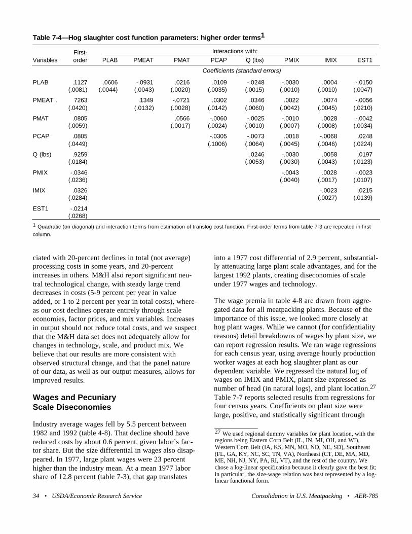
ciated with 20-percent declines in total (not average)processing costs in some years, and 20-percentincreases in others. M&H also report significant neu-tral technological change, with steady large trenddecreases in costs (5-9 percent per year in valueadded, or 1 to 2 percent per year in total costs), where-as our cost declines operate entirely through scaleeconomies, factor prices, and mix variables. Increasesin output should not reduce total costs, and we suspectthat the M&H data set does not adequately allow forchanges in technology, scale, and product mix. Webelieve that our results are more consistent withobserved structural change, and that the panel natureof our data, as well as our output measures, allows forimproved results.

Wages and Pecuniary Scale Diseconomies

Industry average wages fell by 5.5 percent between1982 and 1992 (table 4-8). That decline should havereduced costs by about 0.6 percent, given labor’s fac-tor share. But the size differential in wages also disap-peared. In 1977, large plant wages were 23 percenthigher than the industry mean. At a mean 1977 laborshare of 12.8 percent (table 7-3), that gap translates

into a 1977 cost differential of 2.9 percent, substantial-ly attenuating large plant scale advantages, and for thelargest 1992 plants, creating diseconomies of scaleunder 1977 wages and technology.

The wage premia in table 4-8 are drawn from aggre-gated data for all meatpacking plants. Because of theimportance of this issue, we looked more closely athog plant wages. While we cannot (for confidentialityreasons) detail breakdowns of wages by plant size, wecan report regression results. We ran wage regressionsfor each census year, using average hourly productionworker wages at each hog slaughter plant as ourdependent variable. We regressed the natural log ofwages on IMIX and PMIX, plant size expressed asnumber of head (in natural logs), and plant location.27

Table 7-7 reports selected results from regressions forfour census years. Coefficients on plant size werelarge, positive, and statistically significant through


Table 7-4—Hog slaughter cost function parameters: higher order terms1

First- Interactions with:

Variables order PLAB PMEAT PMAT PCAP Q (lbs) PMIX IMIX EST1


PLAB .1127 .0606 -.0931 .0216 .0109 -.0248 -.0030 .0004 -.0150(.0081) (.0044) (.0043) (.0020) (.0035) (.0015) (.0010) (.0010) (.0047)

PMEAT . 7263 .1349 -.0721 .0302 .0346 .0022 .0074 -.0056(.0420) (.0132) (.0028) (.0142) (.0060) (.0042) (.0045) (.0210)

PMAT .0805 .0566 -.0060 -.0025 -.0010 .0028 -.0042(.0059) (.0017) (.0024) (.0010) (.0007) (.0008) (.0034)

PCAP .0805 -.0305 -.0073 .0018 -.0068 .0248(.0449) (.1006) (.0064) (.0045) (.0046) (.0224)

Q (lbs) .9259 .0246 -.0030 .0058 .0197(.0184) (.0053) (.0030) (.0043) (.0123)

PMIX -.0346 -.0043 .0028 -.0023(.0236) (.0040) (.0017) (.0107)

IMIX .0326 -.0023 .0215(.0284) (.0027) (.0139)

EST1 -.0214(.0268)

1 Quadratic (on diagonal) and interaction terms from estimation of translog cost function. First-order terms from table 7-3 are repeated in first

column.

27 We used regional dummy variables for plant location, with theregions being Eastern Corn Belt (IL, IN, MI, OH, and WI),Western Corn Belt (IA, KS, MN, MO, ND, NE, SD), Southeast(FL, GA, KY, NC, SC, TN, VA), Northeast (CT, DE, MA, MD,ME, NH, NJ, NY, PA, RI, VT), and the rest of the country. Wechose a log-linear specification because it clearly gave the best fit;in particular, the size-wage relation was best represented by a log-linear functional form.

1982. Moreover, unreported coefficients on the Easternand Western Corn Belt locations were positive, signifi-cant, and large. Predicted wages there were substan-tially higher than in the Southeast and the rest of thecountry.

The lower panel of table 7-7 summarizes the estimatedpremia, reporting regression-based predicted hourlywages at Western Corn Belt (WCB) plants for 4 yearsand three different size categories: 400,000 head peryear (sample mean), 1 million head (a large plant for1977) and 4 million head (a large plant for 1992).Compared with the sample mean plant, wages at themillion-head plant were consistently 9-12 percenthigher through 1982, and predicted wages at thelargest plant were 24-33 percent higher. Now note theregional effect of locating in the Southeast (bottomrow); WCB wages are consistently about 50 percenthigher than predicted Southeastern wages through1982. Size and location premia eroded in the unreport-ed 1987 regression, and then disappeared entirely inthe 1992 regression—there are no statistically signifi-cant differences in 1992 predicted wages, and thecoefficient on size is small and not significant. Earlysize and location premia represent a pecuniary scalediseconomy. In the 1980’s and 1990’s, those disec-onomies disappear, reinforcing the effect of changingtechnological scale economies; their disappearancecoincides with sharp increases in plant sizes.

Product and Input Mix Effects

These effects are more complicated in hog slaughterthan in cattle slaughter, where slaughter and carcassfabrication into boxed beef predominate (there is also

processing of byproducts such as hides, blood, andorgans, but we model these as occurring in fixed pro-portions with slaughter). Hog plants slaughter hogsand cut up the carcasses into primals, but many furtherprocess cutup carcasses into hams, sausages, and otherproducts. Our measure of product mix (1 minus theshare of ham and sausage products in plant shipments)aims to capture some important distinctions amongplants. The measure should be closer to 1 in plants thatspecialize more in slaughter and cutup.

The coefficient on PMIX is negative and marginallysignificant for 1992 (table 7-3)—plants that do lessprocessing have lower costs, all else equal.28 Thecoefficient value is not particularly large because pro-cessing costs account for small shares of total costs. Atypical change in product mix toward less processing(from the median 1992 value to the 75th percentile)would lead to a 1.5-percent reduction in total costs,and therefore in average costs per pound. Changestoward less processing also affect factor shares,although only the term involving labor is statisticallysignificant (see the interaction terms with PMIX intable 7-4). Labor and other materials account forsmaller cost shares in plants that do little processing,while animals and capital hold larger shares.

The interaction term between product mix and outputis negative, small, and not nearly significant. That is,the data provide no evidence that costs can be reduced


Table 7-5—Mean input shares and elasticities inhog slaughter1

Input price variables

Item PLAB PMEAT PMAT PCAP

Input shares .1121 .7426 .0779 .0674∈ii -0.347 -0.076 -0.196 -1.385σij

PLAB -3.098 -0.118 3.475 2.443PMEAT -0.102 -0.246 1.602PMAT -2.510 -0.143PCAP -20.55

1 All values are calculated using mean 1992 data values andparameters from tables 7-3 and 7-4. Own-price input demand elas-ticities (∈ii) are calculated holding output and other factors constant,

while the elasticities of substitution (σij) are calculated using Allen'sformula.

Table 7-6—Cost elasticities for differing plant sizesand technology vintages1

Technology vintagePlant size 1992 1977 1963

Sample mean 0.926 .9549 .9856

1992 mean 0.956 0.985 1.0161992 95th percentile 0.983 1.012 1.043



1 The coefficients report the percentage change in total costs corre-sponding to a 1-percent change in output, for plants of differingsizes and technological vintages.

28 Note that this measure carries a different interpretation than thePMIX measure in cattle. Here increases in PMIX mean less pro-cessing; there increases in PMIX mean more processing and fabri-cation.

by combining processing with slaughter in large estab-lishments. That result is reassuring, since evidence ofscope economies would clearly have conflicted withthe observed shift toward separation of slaughter andprocessing in the hog sector.

Our input mix variable is the value share of hogs intotal animal and meat inputs, as distinct from pur-chased carcasses or, in some plants, from otherspecies. The coefficient on IMIX in 1992 is positive,although small and not statistically significant. Notethat the year shifts are all negative (table 7-3), general-ly significant, and usually large enough to make thefull effect negative in the relevant year. That patternprobably reflects changes in input mix over time. In1977, for example, the median value of IMIX was 90percent and the 75th percentile value was 100 percent,but the 25th percentile value was 59 percent. That is,many plants specialized only in hogs, but a substantialfraction of sample plants also purchased large volumeof carcasses, presumably for processing operations. Asthe industry changed over the next 15 years, the distri-bution of IMIX values narrowed, to a median of 98percent and a 25th percentile value of 91 percent.Given the narrow variance of IMIX values in 1992, itshould not be surprising that IMIX has no significanteffect on costs in 1992. In earlier years, with a widervariation in input mix, plants that specialized in hogslaughter realized lower costs.

Few of the individual coefficients involving IMIX andPMIX are statistically significant. That may reflect

multicollinearity between the two measures—plantsthat purchase carcasses also do more processing (ifone variable is dropped, coefficients on the other gainsignificance). Furthermore, it appears that scaleeconomies may be underestimated if the product andinput mix variables are omitted. The estimated scaleelasticity measure rises, by 0.01 to 0.02, for each yearwhen PMIX and IMIX are left out of the estimation.The joint tests of significance (table 7-2) strongly sup-port the inclusion of both measures in the model; as aresult, we believe that economies of scale are bestmeasured when controls for product and input mix areretained.

Conclusion

As in cattle, our estimated cost function finds smallbut important economies of scale at hog slaughterplants. Technological change and a flattening of thesize-wage relation led to greater available scaleeconomies over time, and plants adjusted quickly,growing to take advantage of scale. The industry’slarger plants produce at output levels near constantreturns to scale, but they have not exhausted availableslaughter economies; in consequence, we are likely tosee continued cost pressures on smaller and medium-sized hog slaughter facilities.

The mix of products and inputs at hog slaughter plantshas changed, and plants today are mostly specialized,with a focus on a single species and relatively littleprocessing. Our simple measures of product and inputmix have significant associations with plant costs, so itis important to control for product and input mix whenestimating scale economies and technological change.

We note one other striking similarity with the cattleresults. None of the first-order year intercepts in themodel are large, none are statistically significant, andthere is no particular sign pattern (see the interceptrow in table 7-3). Changes in slaughter costs appear tobe fully accounted for by changes in factor prices (inparticular, by hog prices), changes in input and outputmix, and shifts in plant size to take advantage of scaleeconomies. In turn, productivity growth in hog slaugh-ter operations appears to be driven largely by scaleeconomies.


Table 7-7—Selected results from plant averagewage regressions, by plant size and location1

Item 1963 1972 1982 1992

Coefficient andt statistic on .094 104 .122 .019ln (# of head) (8.40) (7.54) (6.93) (0.91)

Plant characteristics: Predicted wages

Head Location Dollars per production worker hour

400,000 WCB 3.08 5.04 12.17 8.081 million WCB 3.36 5.54 13.61 8.224 million WCB 3.83 6.40 16.11 8.444 million South 2.59 4.20 10.83 8.02

1 Based on regressions of plant average production worker wages(in natural logarithms) on plant size (number of head, in logs). Themodel also included controls for input mix, product mix, and plant

location (Eastern Corn Belt, Western Corn Belt (WCB), Northeast,South, and rest of country).

We organize our conclusions into three sections. First,we summarize our description of the extent of structur-al change in cattle and hog slaughter. Next, we discussthe major findings of the cost analyses, along withtheir implications for cost modeling in slaughter.Finally, we link the two by discussing the impact ofindustry cost structure on structural change.

Structural Change in Cattle and Hog Slaughter

Major consolidation occurred in each industry, as largeplants supplanted small and now dominate production.In each case, the shift to large plants occurred quiterapidly, over a short time period—from 1977 to 1992.Consolidations on such a dramatic and rapid scale arequite rare in U.S. manufacturing.

Consolidation in slaughter proceeded apace with con-solidation in related animal production sectors, as cat-tle feeding shifted toward large commercial feedlotsand hog production shifted toward large hog farms.Because meatpacker procurement generally occursover a limited geographic area, slaughter plants areclosely linked to local feeding and finishing opera-tions. As cattle feeding and hog production shifts geo-graphically, slaughter plants follow. In new areas withlimited networks of producers and slaughter plants,buyers and sellers are less likely to rely on spot marketcash transactions to arrange for the transfer of animals,and more likely to use alternatives such as contractsand vertical integration.

In cattle slaughter, where the demand for cattledeclined through time, consolidation was accompaniedby sharp increases in market concentration, as thenumber of independent plants fell sharply. In hogslaughter, where the market grew slowly, concentra-tion increased, but less so than in cattle. In poultryindustries, where market growth was rapid, concentra-tion changed little despite a consolidation of produc-tion in large plants.

Consolidation was accompanied by important changesin product mix in each industry. Large cattle plants

now ship more output as boxed beef and ground beefinstead of whole and half carcasses, thereby taking ontasks that had been performed in distribution facilities.Hog plants moved to perform a similar set of tasks,but from a different starting point. That is, hog slaugh-ter plants now commonly perform slaughter andbyproduct processing, and also cut carcasses up forshipment much like boxed beef. But many hog plantsused to process carcasses into hams, bacon, sausages,and other prepared products. Specialist processors aremore likely to perform those tasks today.

Slaughter Industry Cost Structure

Our cost analysis emphasized the estimation ofeconomies of scale—the effects of plant size on unitcosts. We found that scale economies were modest butextensive. The largest plants maintained only smallcost advantages (1 to 3 percent) over smaller plants,but these modest scale economies appeared to extendthroughout all sizes of 1992 plants (the last year of ourcost data). The very largest plants in that year did notexhaust all possible scale economies. Still, scaleeconomies were larger and more extensive at the endof the study period (1992) than in earlier years.

Large meatpacking plants traditionally paid higherwages than small, and this pecuniary diseconomy lim-ited the technological cost advantages that scaleeconomies offered large plants. However, size-basedwage premia disappeared during the 1980’s, reinforc-ing the effects of expanding technological scaleeconomies.

The second major emphasis of our cost analysis wason product mix. Product and input mix influencescosts, and mixes vary widely across plants and overtime. Because product mixes are correlated with plantsize (larger cattle plants produce greater proportions ofboxed beef, for example), their omission in models canlead to biased estimates of scale economies and of theextent of technological change and productivitygrowth. Finally, our measures show that there may besmall economies of scope in cattle slaughter, in that


Chapter 8

Conclusions

larger plants can combine slaughter and fabrication atlower cost than smaller plants.

The distinctive feature of slaughter plant operations,compared with other manufacturing operations, is theimportance of materials, particularly animals, in totalcosts. By implication, labor, capital, and energyexpenses form much smaller shares of costs in slaugh-ter industries than elsewhere. It is this importance thatensures that scale economies have modest effects oncosts, because scale economies primarily arise in theuse of other inputs—labor, capital, and energy—atslaughter plants. Moreover, although there is some the-oretical scope for substitution between animals andother inputs in the production of meat, our analysesshow that there is virtually no actual substitution; onecan reasonably estimate “value-added” cost functionsfor slaughter under the assumption of no substitution.

From Costs to Structure: Did ScaleEconomies Cause Consolidation?

Our evidence shows modest scale economies in cattleas well as hog slaughter: large plants can produce meatat slightly lower costs than small slaughter plants.These advantages became more important in the1980’s, as the industries consolidated and productionshifted to large plants. That is, the existence of scaleeconomies, and the timing of their appearance, sug-gests that consolidation occurred because of scaleeconomies.

But scale economies cannot be a complete explanationfor consolidation because the cost advantages held bylarge plants are not particularly large. Small plantsappear to survive, and consolidation is staved off, inmany industries with larger scale economies than thosefound in meatpacking (see, generally, the discussion inMcKinsey Global Institute, 1993, or its related sum-mary in Baily and Gersbach, 1995). For modest scaleeconomies to lead to consolidation as massive as thatin meatpacking, the industry was likely subject tostrong price competition. That is, small plants willclose if market prices are below small plant unit costs;for market prices to be below small plant costs, theymust in turn be quite close to large plant unit costs,due to small differences between small and large plantunit costs.29

The labor strife of the 1980’s, as reported in chapter 4,may also reflect strong price competition in the indus-try. While unionized plants had substantially higherwages than nonunion plants in the 1970’s, the effecton costs would be small because the share of wages intotal costs was small. For small cost differences tolead to plant closures and lockouts, the higher costunionized plants would have to have been under strongcompetitive price pressures from the nonunionplants.30

Our conclusions about price competition in slaughtermust be more speculative, because they are based noton our own work but on the published literature, withfar more information for cattle than for hogs. Theexisting literature suggests that departures from com-petition in cattle slaughter have been small and rare. Incompetitive markets, product prices should equal mar-ginal costs of production, while prices paid for inputs(like cattle) will equal the value of the input’s marginalproduct. Attempts to measure departures from compe-tition take two forms. Researchers may attempt todirectly estimate the gap between prices and the corre-sponding competitive magnitudes (marginal costs ormarginal value products), relying on the econometricestimation of demand and cost models. Alternatively,they may attempt to see if prices vary systematicallywith variations in competitive conditions, while tryingto hold (or assuming) constant other cost and demandfactors.

Most early studies took the latter approach. For exam-ple, Marion and Geithman (1989) examined howprices paid for slaughter cattle varied with buyer con-centration across buying regions, while also control-ling for interregional differences in labor costs andinterseller differences in feedlot size. They found thatbuyers in more concentrated markets paid less for cat-tle, but that the differences were small: prices for cat-tle fell by 3.4 percent, at most, as one moved from theleast concentrated to the most concentrated region.Other early studies, surveyed by Azzam and Anderson(1996) found similar results: concentration effects, ifthey existed, were small.

More recently, the Texas A&M Agricultural MarketResearch Center (1996) used far superior data to arrive


29 Strictly speaking, average variable costs, but variable costs inmeatpacking are very close to average total costs.

30 Large plants may also realize marketing advantages over small-er plants through export markets and nationwide shipping.However, marketing advantages are difficult to identify in thesedata sets (or in other existing ones).

at a familiar conclusion. They were able to control fora wide array of cost, cattle characteristic, and demandmeasures, and found that prices paid for cattle in 1992were lower in more concentrated regions, but that cat-tle prices fell by only 2.4 percent as one moved fromthe least to the most concentrated market. Moreover,the most concentrated regions in these studies areremote areas that host some relatively small plants.The less concentrated regions are the areas of consoli-dation of large plants in the Plains: there, prices areslightly higher.

Studies that rely on direct estimation of gaps betweenprices and corresponding competitive values reachedsimilar conclusions. Those based on reliable estima-tion of demand and cost functions may disagree as towhether prices equal competitive magnitudes, but nonefound large departures of prices from those magni-tudes. For example, Morrison (1998) found that prod-uct prices exceed marginal costs of production (thecompetitive magnitude) by a small gap, 5 to 10 per-cent, which indicates that plants had very limited mar-ket power in product (wholesale meat) markets. Shefurther found that prices paid for animals in input (cat-tle) markets were not below competitive levels.

Finally, measures of farm-to-wholesale price spreadsdid not increase over time as concentration increased.The aggregate USDA measure of the farm-to-whole-sale price spread for choice beef reflects transporta-tion, slaughter, and fabrication costs (Nelson andHahn, 1998). Adjusted for inflation, the spread fluctu-ated during the 1970’s, but fell steadily and sharplyfrom 1979 through 1992, the period of sharpest con-solidation, even as plants added more fabrication andthe attendant costs. Farm-to-wholesale margins did

rise sharply between 1992 and 1995, but then fell backagain in 1996 and 1997.

Several factors, whose effects are difficult to measure,may have helped to increase concentration in meat-packing—these include economies of operating multi-ple plants, large firm marketing advantages (particular-ly in exports), and mergers among packing firms. Butif the pricing evidence is correct, then the followingthree measurable factors clearly combined to helpincrease concentration in cattle slaughter: (1) shifts inscale economies provided larger plants with modestcost advantages; (2) aggressive price competitionforced prices to quickly move near the costs of thelow-cost market participants; and (3) slow demandgrowth limited the number of efficient large plants inthe market. In hogs, scale economies and strong pricecompetition have also forced small plants to exit theindustry, but faster demand growth allowed for moreplants and lower concentration.

Our evidence suggests that once new and extensivescale economies emerged in meatpacking, intenseprice competition led to the exit of high-cost smallplants, their rapid replacement by larger and more effi-cient plants, and significant increases in market con-centration. The policy challenge for the future is toensure that a result of the process, high concentration,does not erode a key contributing factor—price com-petition among packers. The analytical challenge is tocontinue to update the evidence so that we can effec-tively monitor competitive conditions in an industrythat is now concentrated, and to ensure that we ade-quately understand the causes and effects of continuedchange in the industry.


40 • USDA/Economic Research Service Consolidation in U. S. Meatpacking • AER-785

Allen, W. Bruce, and Dong Liu, “Service Quality and MotorCarrier Costs: An Empirical Analysis,” Review ofEconomics and Statistics 77 (Nov., 1995): 499-510.

Azzam, Azzedine M., and Dale G. Anderson, AssessingCompetition in Meatpacking: Economic History, Theory,and Evidence. U.S. Department of Agriculture; GrainInspection, Packers and Stockyards Administration.Technical Report No. GIPSA-RR 96-6. May 1996.

Baily, Martin Neil, and Hans Gersbach, “Efficiency inManufacturing and the Need for Global Competition,”Brookings Papers on Economic Activity: Microeconomics(1995): 307-347.

Ball, V. E., and R.G. Chambers, “An Economic Analysis ofTechnology in the Meat Products Industry,” AmericanJournal of Agricultural Economics 62 (Nov. 1982): 699-709.

Baltagi, Badi H., James M. Griffin, and Daniel P. Rich,“Airline Deregulation: The Cost Pieces of the Puzzle,”International Economic Review 36 (Feb. 1995): 245-258.

Berndt, Ernst R., The Practice of Econometrics: Classic andContemporary (New York: Addison Wesley Publishing,1991).

Brown, Charles, James Hamilton, and James Medoff,Employers Large and Small (Cambridge, MA: HarvardUniversity Press, 1990).

Caves, Douglas W., Laurits R. Christensen, Michael W.Tretheway, and Robert J. Windle, “Network Effects andthe Measurement of Returns to Scale and Density for U.S.Railroads,” in Andrew F. Daugherty, ed., AnalyticalStudies in Transport Economics (Cambridge, UK:Cambridge University Press, 1985).

Chambers, Robert G., Applied Production Analysis: A DualApproach (Cambridge, UK: Cambridge University Press,1988).

Crom, Richard J., Economics of the U.S. Meat Industry.U.S. Department of Agriculture. Economic ResearchService. AIB-545. Nov. 1988.

Curme, M.A., Barry T. Hirsch, and David A. McPherson,“Union Membership and Contract Coverage in the UnitedStates, 1983-1988,” Industrial and Labor RelationsReview 44 (Oct. 1990): 5-30.

Drabenstott, Mark, “This Little Piggy Went to Market: Willthe New Pork Industry Call the Heartland Home?”Federal Reserve Bank of Kansas City Economic Review,Third Quarter 1998: 79-97.

Duewer, Lawrence A., and Kenneth E. Nelson, Beefpackingand Processing Plants: Computer Assisted Cost Analysis.U.S. Department of Agriculture, Economic ResearchService, Staff Report AGES 9115. April 1991.

Feder, Barnaby J., “The Stew Over Beef,” New York Times,Oct. 17, 1995.

Gallant, A. Ronald, and Dale W. Jorgenson, “StatisticalInference for a System of Simultaneous, Non-Linear,Implicit Equations in the Context of Instrumental VariableEstimation,” Journal of Econometrics 11 (Nov. 1979):275-302.

Glover, Teresa, and Leland Southard, “Cattle IndustryContinues Restructuring,” Agricultural Outlook 238 (Dec.1995): 13-16.

Hayenga, Marvin L., Stephen R. Koontz, and Ted C.Schroeder, Definition of Regional Cattle ProcurementMarkets. U.S. Department of Agriculture; GrainInspection, Packers and Stockyards Administration.Technical Report No. GIPSA-RR 96-1. May 1996.

Hayenga, Marvin L., “Cost Structures of Pork Slaughter andProcessing Firms: Behavioral and PerformanceImplications,” Review of Agricultural Economics 20(Fall/Winter 1998): 574-583.

Hedges, Stephen J., and Dana Hawkins, “The New Jungle,”U.S. News and World Report, Sep. 23, 1996: 34-45.

Johnson, Dirk, “Growth of Factory-Like Hog Farms DividesRural Areas of the Midwest,” New York Times, June 24,1998: A12.


References

Kambhampaty, S. Murthy, Paul J. Driscoll, Wayne D.Purcell, and Everett B. Peterson, Effects of Concentrationon Prices Paid for Cattle, U.S. Department of Agriculture;Grain Inspection, Packers and Stockyards Administration.Technical Report No. GIPSA-RR 96-4. June 1996.

Kokkelenberg, Edward C., and Donna R. Sockell, “UnionMembership in the United States, 1973-1981,” Industrialand Labor Relations Review 38 (July 1985): 497-543.

Lawrence, John, Glenn Grimes, and Marvin Hayenga,“Dramatic Changes Occurring in the U.S. Pork Productionand Marketing Systems,” unpublished manuscript,University of Iowa, Nov. 1998.

MacDonald, James M., Michael E. Ollinger, Kenneth E.Nelson, and Charles R. Handy, “Structural Change inMeat Industries: Implications for Food SafetyRegulation,” American Journal of Agricultural Economics78 (Aug. 1996): 780-785.

Marion, Bruce W., The Organization and Performance ofthe U.S. Food System (Lexington, MA: Lexington Books,1986).

Marion, Bruce W., and Frederick Geithman, “Live CattlePrices and Packer-Buyer Concentration,” in Leonard W.Weiss, ed., Concentration and Price (Cambridge, MA:The MIT Press, 1989)

McBride, William D., U.S. Hog Production Costs andReturns, 1992: An Economic Basebook, U.S. Departmentof Agriculture, Economic Research Service, AER-724.Nov. 1995.

McBride, William D., Changes in U.S. LivestockProduction, 1969-92. U.S. Department of Agriculture,Economic Research Service, AER-754. July, 1997.

McKinsey Global Institute, Manufacturing Productivity.Report prepared with the assistance of Martin Baily,Francis Bator, Ted Hall, Robert Solow, and the Universityof Groningen. Washington, DC. Oct. 1993.

Melton, Bryan E., and Wallace E. Huffman, “Beef and PorkPacking Costs and Input Demands: Effects ofUnionization and Technology,” American Journal ofAgricultural Economics 77 (Aug. 1995): 471-485.

Morrison, Catherine, “Cost Economies and Market Power inU.S. Meat Packing,” report to the U.S. Department of

Agriculture; Grain Inspection, Packers and StockyardsAdministration. Feb. 1998.

Nelson, Kenneth E., and William Hahn, “Concentration inthe U.S. Beef Packing Industry,” Livestock, Dairy, andPoultry Situation and Outlook, U.S. Department ofAgriculture, Economic Research Service, LDP-M-53 ,Aug. 17, 1998: 10-22.

Ollinger, Michael E., James M. MacDonald, and MiltonMadison, “Structural Change in U.S. Chicken and TurkeySlaughter,” U.S. Department of Agriculture, EconomicResearch Service, unpublished manuscript, Dec. 1999.

Putnam, Judith Jones, and Jane E. Allshouse, FoodConsumption, Prices, and Expenditures, 1970-95. U.S.Department of Agriculture, Economic Research Service,SB-939. Aug. 1997.

Sersland, Claudia J., “Cost Analysis of the Steer and HeiferProcessing Industry and Implications on Long-RunIndustry Structure.” Unpublished Ph.D. dissertation,Oklahoma State University. Dec. 1985.

Sutton, John, Sunk Costs and Market Structure: PriceCompetition, Advertising, and the Evolution ofConcentration. Cambridge, MA: The MIT Press, 1991.

Texas A&M Agricultural Market Research Center. PriceDetermination in Slaughter Cattle Procurement. UnitedStates Department of Agriculture; Grain Inspection,Packers and Stockyards Administration. Technical ReportNo. GIPSA-RR 96-2. May 1996.

U.S. Department of Agriculture, Agricultural MarketingService. Concentration in Agriculture: A Report of theUSDA Advisory Committee on Agricultural Concentration.June 1996.

U.S. Department of Agriculture, Economic ResearchService, Red Meats S&O Yearbook. SB-921. Nov. 1995.

U.S. Department of Agriculture; Grain Inspection, Packersand Stockyards Administration, Packers and StockyardsPrograms. Concentration in the Red Meat PackingIndustry. Feb. 1996.

U.S. Department of Agriculture; Grain Inspection, Packersand Stockyards Administration, Packers and StockyardsPrograms. Packers and Stockyards Statistical Report:1997 Reporting Year. GIPSA Statistical Report SR-99 -1.Sep. 1999.


U.S. General Accounting Office, Changes in Nebraska’s andIowa’s Counties with Large Meatpacking Workforces.GAO/RCED-98-62. Feb. 1998.

Ward, Clement E., “Meatpacking Plant Capacity andUtilization: Implications for Competition and Pricing,”Agribusiness 6 (Jan. 1990): 65-73.

Ward, Clement E., “Comparative Analysis of CattleSlaughtering and Fabricating Costs,” Agribusiness 9 (Sep.1993): 441-451.


consolidation in u.s. meatpacking - usda

Documents