constant pressure molecular dynamics algorithms -...

Constant pressure molecular dynamics algorithms Glenn J. Martyna Department of Chemistry, Indiana University, Bloomington, Indiana 47405-4001

Douglas J. Tobias and Michael L. Klein Department of Chemistry, University of Pennsylvania, Philadelphia, Pemnsylvania 19104-6323

(Received 19 January 1994; accepted 18 May 1994)

Modularly invariant equations of motion are derived that generate the isothermal-isobaric ensemble as their phase space averages. Isotropic volume fluctuations and fully flexible simulation cells as well as a hybrid scheme that naturally combines the two motions are considered. The resulting methods are tested on two problems, a particle in a one-dimensional periodic potential and a spherical model of C,, in the solid/fluid phase.

1. INTRODUCTION

In the past decade, equations of motion have been developed that generate many-body thermodynamic ensembles as their phase space averages.lw6 Alternatives to Monte Carlo methods are, now, available to study systems in the canonical, isothermal-isobaric, and isoenthalpic-isobaric ensembles.

Recently, the isobaric methods have been reexamined.6 It was observed that while isobaric ensembles are produced, the trajectories have an unphysical dependence on the choice of basis lattice vectors?” This behavior arises because the equations of motion are not modularly invariant.7*8 However, modular invariance can be incorporated naturally into isobaric schemes using the formalism developed by Hoover.4*6*9 In this yafer, the inconsistencies of prior schemes are removedh4 6*9 and a new hybrid method which combines both isotropic volume fluctuations and full flexibility of the simulation cell is introduced. The methods are tested on two model problems, a particle in a one-dimensional periodic potential and C6s molecules in the solid/fluid phase.

il. ISOTHERMAL-ISOBARIC ENSEMBLE

In this section, three different approaches that generate the isothermal-isobaric ensemble are explored: uniform dilation, full flexibility of the simulation cell, and a hybrid scheme.

A. Uniform dilation

The equations of motion proposed by Hoover have the following basic form for a d-dimensional system of N particles (yf degrees of freedom; Nf=dN if there are no constraints):4~9~*0 &=pI +E ri,

mi W

dVPE c=- P@e w ) li.=dWint- P,,,) --yj- I

* P? P’, “=; , &=x k +w-(Nf+ 1)kT.

ill

Here, ri and pi are the position and momentum of the ith particle, V is the volume, pE is the barostat momentum, c and pc are the thermostat position and momentum, F,= -V,$(r, V) is the force, Pext is the external/applied pressure, and

N p2 N

7 ; + C ri.Fi--(dV) c=l z i=l

y (2.2) 1 is the internal pressure. A possible explicit dependence of the potential energy on the volume has been considered. Such terms will occur when long-range interactions [ 4( I-) CC 1 lrn,n G3] or long-range corrections to short-range potentials are present. Cutting off long-range interactions or neglecting long-range corrections in small systems can give rise to incorrect results.” Note that the barostat momentum pe has been coupled to the thermostat momentum pg.

Hoover’s equations have the advantage that they automatically and naturally satisfy the constraint that the volume be greater than or equal to zero, namely, V(t)= V(O) Xexp[d/WJ@t’ p,(t’)]. The equations also have the conserved quantity

N 2

H’=x -!?- +p: +% +&r,V)+(Nf+l)kT~ i=, 2mi 2W 2Q

+ pextv, (2.3)

~ =~ [V,H’.~i+V~iH”iil+~Pi+~ ~ i=l

+$ de+% Fi=o, e

and Jacobian,‘2

di dkc d’li dfi, - +-- f- +- d5 dpt dV dp,

N

+C (Vpiii+Vriti) i=l

J(t)=V-l exp[(Nf+ l)f].

J. Chem. Phys. 101 (5), 1 September 1994 0021-9606/94/l 01(5)/4177/13/$6.00 Q 1994 American Institute of Physics 4177 Downloaded 21 Sep 2009 to 131.104.62.10. Redistribution subject to AIP license or copyright; see http://jcp.aip.org/jcp/copyright.jsp

4178 Martyna, Tobias, and Klein: Constant pressure molecular dynamics algorithms

The Jacobian is the weight associated with the phase space volume and is unity for systems that obey Liouville’s theorem.12 It represents the transform to a set of variables where J= 1, here, simply, {i = Nfsp$ or equivalentry, {log s = N#}. Using the assumption of ergodicity, the Jaco- bian, and the conserved quantity, the partition function associated with the dynamics can be constructed:12

;.=.E +p’ r. L mi w ”

isoenthaIpic-isobaric ensemble is produced to within the fluctuations of Wp’,, the barostat kinetic energy.

In this paper, the alternative equations of motion are proposed:

A= dpc dp, dE dV I

Dcndp dr V-l I”

dvp, v=- N P: PE w ’ d.=dV(Pint-PexJ+$ F G-Qpe,

I 1

exp[ ElkTj A=cNf+ ljkT

H” Xexp --E, [ 1

where

(2.9)

N P: P”, “=$ , r;,=c m- +F-(Nf+ 1)kT. i=] 1

N

HN=x -!f- +p: +& ++(r,V)+P,,V i=l 2mi 2W 2Q (2.6)

and D(v) is the domain defined by the volume. Unfortu- nately, A is not the isothermal-isobaric partition function (within a constant) as was made clear by Hoover in the original derivation?Tg

Like the prior modification, Eqs. (2.7), the new equations, Eqs. (2.9), have the same conserved quantity as Hoover’s original set, Jacobian, J=exp[(Nf+l)c] and, in principle, generate the isothermal-isobaric partition function (within a constant). Again, if the thermostats are removed, the isoenthalpic-isobaric ensemble is produced to within the fluctuations of Wpz.

In an effort to correctly generate the isothermal-isobaric ensemble, it has been suggested that Hoover’s equations of motion be slightly modified?

The relative merits of the modified equations of motion, Eqs. (2.7), and th e new equations of motion, Eqs,. (2.9), must be assessed. A simple physical argument based on the conditions for equilibrium in a dynamical system will be given in the text. A complete and rigorous analysis of the phase space is provided in Appendix A.

St=2 +k (ri-rc.m.), I

&=Fi-g pi--z pi,

dvp, UP.-- PPP, w ’ I;e=dV(~int-Pe,t)-~ 7 (2.7)

N PZ “=$, I;,=c m- +$-(Nf+ l)kT,

i=l ‘

where r,., - -( l/M)Xirniri is the center of mass (c.m.) and

C ; + 5 Iri-rc.d*Fi N pf

ia, z- i=l

JHr,V) -(dV) 7

I

. W)

If a dynamical system is at equilibrium, the time average of the force on each of the independent variables will be zero. Furthermore, if the system is: ergodic than the time average can be taken to the trajectory average. Application of this principle to Hoover dynamics, Eqs. (2.1), yields

(i)c)=d((Pi,t-P,,t)V)=O, (2.10)

a statement of a pressure virial theorem obeyed by the Hoover ensemble, Eq. 2.5 (see Appendix B for a discussion of pressure virial theorems). Unsurprisingly, there is a feed- back between the equations of motion and the equilibrium/ limiting distribution function. Similarly, the equations of motion proposed in this paper, Eqs. (2.9), generate

(ad=d( (6 T g) + (CPint-P,JV)] =O-

These equations have the same conserved quantity as the original set, but the Jacobian is J=exp[(Nf+ l)[]. The isothermal-isobaric ensemble is, therefore, in principle, generated. For the special case of no external forces, Q,,.=O, considered in the original paper,6 the choice Pint=Pint was made. Note, another, possible but nonseparable choice is P,,=X~= 1 (ri - r,,) ’ SF: , where a prime indicates that a given term must be consistent with the periodic boundary conditions. For the more restrictive case of a set of free particles, both choices reduce to, Pint=~int. Most generally, however, the two functions, Pint and I?int, are not equal. If the thermostats are decoupled from the dynamics, the

a virial theorem obeyed by the isothermal-isobaric ensemble (see Appendix B). The rather strong condition, the kinetic virial theorem, is used to produce the necessary factor of kT. The modified equations, Eqs. (2.7), give

(li.)=d{((~i~t-Pi,)V)+((Pi,-P,,)V)}=O. (2.11)

Here, ((~,-P,)V)=(l/d)(r,.,..F,.,~ (the definition of the pint from the original papeP) is relied upon to generate the crucial factor of kT. If this term is zero, then in order to achieve a stable equilibrium the Hoover ensemble, Eq. (2.3, must be produced.

J. Chem. Phys., Vol. 101, No. 5, 1 September 1994

Downloaded 21 Sep 2009 to 131.104.62.10. Redistribution subject to AIP license or copyright; see http://jcp.aip.org/jcp/copyright.jsp

0 0.2 0.8 1

0 0 0.2 0.4 0.6 0.8 1

10~ v (A')

FIG. 1. (a) Volume distribution function of a system of ten free particles (I”=300 K, P,,= 100 atm, M=3) with total linear momentum conservation. (b) Volume distribution fimction of a system of ten free particles without momentum conservation. The solid line is the exact result, the short dashed line is the result of Eq. (2.1) or (2.7), the long dot dashed line is the result of E!qs. (2.9).

The analysis based on the virial theorem seemingly con- tradicts the proof based on the Lioville equation (see above) for the modified equations of motion if F,,.=O, ~int=Pint. However, under these conditions, the position of the center of mass of the particles is an auxiliary variable, i.e., the dynamics of the r,.,. depend on all the other variables but not vice versa. In such dynamical systems, satisfying the Liou- ville equation for the entire distribution is insufficient to guarantee that the individual pieces are properly generated. In Appendix A, it is shown that for systems with no external forces, the volume distribution generated by Eqs. (2.7) is reduced by one factor of the volume. In Fig. 1, the pathology is illustrated numerically, for a system of free particles, with and without the imposition of a zero linear momentum con- s@ah pc.m =O. In the numerical calculations, the Nose- Hoover thermostatting scheme, which is insufficient to handle the condition &,(t)#O, F,.,.=O),13924 is replaced by the more general Nose-Hoover chain methodi (see Ap- pendix C).

d(V)=] d& Q(V,&)S(det&]- 1)

= di;, I s &),V) dp dr exp[ - PHhdl

X S(det[&]- l), (2.14)

where the domain-of integration is determined by the trans- formation r= V”dh,p, where s are the scaled/reduced coordi- nates. The assumption, consistent with the isothermal- isobaric ensemble, is that all cells with the same volume OCCUT with equal a priori prgbability weighted by the appropriate Boltzman factor Q (V,b). Therefore, the virial theorem is always obeyed, i.e., the external pressure P,,, is directly related to the average of the usual expression for the internal pressure and the correct isotropic limit is obtained.

It is possible to transform the proposed partition function, Eq. (2.13), to a more familiar_ form. ,By introducing the normal matrix of cell parameters, h = V”‘dh,, , and eliminating the volume using the delta function, one finds

I

A= J

dG exp[-PP,,, det($]Q($det[c]‘-d. (2.15)

In this form, it is possible to show that the tensorial virial theorem

8 W Q 6 )l Pap-Pext~ap)=

dh,l

The results presented above and in Appendix A suggest that the new equations of motion, Eqs. (2.9), will be robust while the modified equations, Eqs. (2.7), may fail to generate the isothermal-isobaric ensemble under certain circum- stances, particularly, if the separable definition of lint (Ref. 6) is employed. Therefore, the new equations of motion, Eqs. (2.9), appear to be superior. Tests of the new method on more realistic problems are described in Sec. IV.

is satisfied and, hence, this indicates that Eq. (2.15) is the appropriately generalized isothermal-isobaric partition function. Equation (2.15) is slightly different from the ensemble that has been used most commonly in simulations, namely,

A= I

di exp[-PP,, det(L)]Q(G). (2.17)

The tensorial virial theorem satisfied by Eq. (2.17),


Martyna, Tobias, and Klein: Constant pressure molecular dynamics algorithms

B. Fully flexible cells

4179

It is often useful to consider not only isotropic relaxation but full relaxation of the simulation ce11.2,5 In order to ac- complish this, an ensemble with anisotropic cell fluctuations must be introduced. The general result

A= s dV evil--PP,,,Vlb(V), (2.12)

where Q(V) is a canonical partition function, can be rewrit- ten as

A= I

dVd& exp[-/3P,,V]Q(V,~o)S(det[&]-1).

(2.13)

Here,


(2.18)

is inconsistent with the isothermal-isobaric ensemble. Note that Eq. (2.15) is only valid for isotropic pressure. The fully nonlinear formulation of the constant tension ensemble which satisfies an appropriate tensorial virial theorem different from Eq. (2.16), and introduces a fixed reference lattice, has been discussed elsewhere.’ Here, the generalized isothermal-isobaric ensemble, Eq. (2.15) will be used. This is a fully nonlinear treatment of the case that isotropic tension is applied along the instantaneous lattice vectors.i5

The equations of motion necessary to produce the desired ensemble, Eq. (2.15), are

N Pf &=$, PF;=c 6 +$ Tr[j$s]-(Nf’-t-d’)kT, i=l g uu

where V-degh], 1 is the-identity matrix, Tr[$&] is the sum of the squares of all the elements of the matrix, 5s; and

+ (FJ,(rJp-

defines the pressure tensor. The modularly invariant form of the box momenta & are taken from earlier work.6,7,‘6 These

& bi=Fi-$ pi-

go equations of motion have conserved quantity:

dvp, 2

Tr[ss&] +$ + ~$(r,c) e=- )

+ P, det[P]+(Nr+d’)kTe (2.22)

and Jacobian, J=det[K]’ -’ exp[(Nf + d2) t]. This leads to the partition function

dp< d: d& I

- dp dr det[G]*-d DC4

> (2.23)

where N 2

Ht&c pi + --ii- Tr#$s] +g + +(r,i;) i=, 2% 2Wg

-I- P, det[K]. (2.24)

The equations of motion reduce to the uniform scaling case when d = 1 and are modularly invariant. They also au-

tomatically and naturally satisfy the constraint that the volume det[h] be greater than_ or equal tg zero, Tr [ss] = W~ij~iihjt * = (W,/det[h])Cijhii(d det[h]/dhij ) =W,log(det[h]). In addition, if the thermostat is decoupled, the isoenthalpic-isobaric ensemble is recovered.

As stated above, the quantity Tr[&] is equal to Wg log(V) and is therefore related to PE of the previous set- tion. In analogy with de, the average of d Tr[&]/dt obeys the virial theorem (see AppendixB)

=dkT+d(V(Pi,-P,,,))=O


(2.25)

and each of the individual & satisfy the tensorial vi&l theorem

(2.26)

C. Hybrid method

It is possible to separate out the isotropic volume flue- tuations from other changes in the simulation cell. Such a separation allows different time scales to be associated with the two types of motion (isotropic and anisotropic) through introduction of different masses for the independent momenta. This separation also-makes it easy to change from a fully flexible cell to an isotropically flexible cell within the same computational framework. Such an approach is only useful for d > 1.

In order to separate out the isotropic fluctuations, the following equations of motion are proposed:

/j =dV(p. -p E mt

- iigoLl (2.27)

g)=- Wgo ’ .

N pf pz Pt=c pn. -l-v +$- Tr[FQ$&j-(@f+d”)kT,.

is1 L gn

where V”“&=c, the instantaneous pressure Pint is given by Eq. (2.4), and the pressure tensoris given by Eq. (2.20). The necessary condition that the det[ha] remain equal to one is



automatically satisfied provided Tr[$d is initially zero as log(det&]) = Tr[&]. Therefore, the ha have no dynamics for d<2.

The conserved quantity for the equations of motion, Eqs. (2.27), is _(_,

2 2

Tr[ 3so$,] + Pe + pg 2w 2Q

+d(r,v,i;,)+P,,V+(Nf+d”)kT~ (2.28)

and the Jacobian is J=exp[(Nf+ d*) t]. The new dynamical equations lead to the partition function

exp[ElkT] h=(Nf+d’)kT j- dp t dp e dV di;, d&,

H” X

J &v) dp dr exp [ 1 - k~ S( det[ :a] - 1 j

x Wr[&,& (2.29)

H”=; & +L Tr[~go$+$ +$ i=l 2mi 2Wgo

+ q%r, V&l + P,,,V. (2.30)

If the thermostat is decoupled, the isoenthalpic-isobaric ensemble is recovered. Also, virial theorems are satisfied by (P6) and (&). Note, ,that both the dynamics and the ensemble produced by the hybrid method are equivalent to the preceding formulation. However, the hybrid method can be a computationally convenient scheme.

D. Elimination of cell rotations

The equations of motion for the case of .a flexible-simulation cell were-derived using thy full matrix of Cartesian cell parameters h or equivalently h,. The cell can therefore, in general, rotate in space.’ This motion can make data analysis difficult and should be eliminated.

The origin of the rotational motion of the cell lies in pressure tensor, Pap [see Eq. (2.20)]. If the instantaneous value of the components of the pressure tensor are asymmet- ric, p,p+ ppp, then there will be a torque on the cell that will cause it to rotate. This suggests that there are two options that can be used to eliminate the rotations. The tirst is to work with the symmetrized tensor P+= (P,+ P&/2. Here, if the total angular momentum of the cell is initially zero, the cell should not rotate. A second option is to work with a restricted set of cell parameters that only respond to the upper/lower triangle of the tensor. This freezes the rotations out.

It is possible to implement either of these two options within both of the sets of equations of motion derived for fully flexible cells, i.e., the normal method, Eqs.. (2.19), and the hybrid method, Eqs. (2.27). The application to the symmetrized tensor will be considered first. Here, the constraint g-=2 in the normal method or &=za in the hybrid method

must be introduced to the dynamics through the use of Lagrange multipliers. (Note, 2 and :a are defined by the time integrals of W,; = & and W$,, = &,, respectively.) Elimi- nating the multipliers results in the replacement of Pap by P,;. in Eqs. (2.19) and (2.27). In the normal method, the constraint imposes the conservation laws

d&-$.1 =. w dJtot dt + &?dt=

o

in two dimensions and

d&-$1 =. w 4iJtotl & - &?dt=’

(2.3 1)

(2.32)

in three dimensions where the Jtot are the components pf the total angular momentum of the cell and the identity &, . = WgEvl has been used. In the hybrid method, the imposed conservation laws are

:

Martyna, Tobias, and Klein: Constant pressure molecular dynamics algorithms 4181

4&, - $,,I dt

=o~ w W-‘&l go dt =’

I .

in two dimensions and -

“[ii;p,- F&l dt

=. w ,dCV- ‘i;J,tl go dt

=o

(2.33)

(2.34)

in three dimensions. The only solution consistent with initial condition $a = Fs or Es0 = Fs, is Jtot=O. The conservation laws guarantee that Jtot will remain zero and the cell will not rotate (i.e., a fixed point of the dynamics is utilized).

The application to the case of an upper triangular cell is also simple. Here, the constraint that hii=O, i>j or (h,)ij=O, i>j must be enforced. Introduction and elimination of the Lagrange multiphers reveals that only the upper triangle of the equations of motion need to be considered. This is obvious since upper triangular matrices form a’closed algebra. It should be noted that the dynamics produces the ensemble

A= dVd&, exp[-PP,,,V]Q(V,&)S(det[&]-lj f

d

Xl-I UkJ;;‘, I=1

(2.35)

A= I

dc exp[-PP,,, det(z)]Q(c)

d

Xn (II);,’ decg]‘-d, I=1

where the space of the h@ has been weighted to account for the unequal a priori sampling of the upper triangular form. In this space, the tensorial virial theorem

J. Chem. Phys., Vol. 101, No. 5, 1 September 1994 Downloaded 21 Sep 2009 to 131.104.62.10. Redistribution subject to AIP license or copyright; see http://jcp.aip.org/jcp/copyright.jsp

-p&&p = 0 (2.36)

is obeyed where p3~. Using the form of the canonical partition function, it can be shown Pap is still given by Eq. (2.20). However, if the matrix of cell parameters is constrained to be symmetric, the pressure tensor that satisfies the virial theorem is no longer given by Eq. (2.20). This third option is therefore to be avoided.

The two methods outlined above will eliminate rotations of the simulation cell. In both methods, however, some in- formation about the behavior of the off-diagonal components of the pressure tensor has also been eliminated. Therefore, the average of all the off-diagonal components of the pressure tensor should be monitored to ensure that each is independently equal to zero. This is more physically meaningful when the method based on the symmetrized tensor is-used because the weight associated with the space of the h, remains uniform. The symmetrized method must therefore be considered a somewhat better way to eliminate rotations of the simulations cell. [On a technical note, the quantity Nf+d” that appears in the equations of motion for pE must be changed to LV~+ d(d+ 1)/2 in the upper triangular case.]

E. Temperature control

In the equations of motion written above, a single thermostat was coupled to the particles and volume/cell variables. While this scheme is usually effective it does not always perform well. For example, large periodic oscillations in the total kinetic energy were found to develop in protein simulations.17 Also, the equations of motion are not always ergodic4 The Nose-Hoover chain method has been developed to overcome these difficulties.14 In this method, the thermostats themselves are thermostatted to form a chain:

(2.37) IV. RESULTS I’e,= Qj-, kT -pcj G ’ [ 1 Pii-, ‘cj+l p:wmi -- ‘SEA= [ 1 --kT , QM-I Two model problems were used to test the new methods

proposed herein: a particle in a one-dimensional periodic potential and C6a molecules in the bulk solid/fluid phases.

where M is the chain length. Therefore, in actual simulations, it is useful to thermostat the particles using a Nose- Hoover chain. It is also useful to use an independent chain to thermostat the volume/box variables to ensure these stiff variables properly sample the phase space. These additions are completely consistent with the results presented above. However, if constraints on the particle degrees of freedom are introduced, the volume/box variables and all degrees of freedom involved in the constraints, must share the same thermostat (see Appendix D).


F. Mass choice of the extended variables

It has been shown elsewhere3.i4 that the masses of the particle thermostats should be taken to be QP1 = NfkT/w$ QPi = kTloi, where wP is the frequency at which the particle thermostats fluctuate. SimilarIy, the masses of the barostat/ cell parameter thermostats should be taken to be Qb, = d(d + ljkT/2w% for the upper triangle case, Qb, = d’kTlwt for the symmetric case, and Qbi = kTlw% in general. (It has been assumed that the particles and the barostats are independently thermostatted.) The masses of the barostat/ cell parameters themselves3*6 should be taken to be W=(Nf+d)kTlw,2, Wg= Wgo=(Nf+d)kTldo;.

Ill. VELOCITY VERLET BASED lNTEGRATORS

A treatment of the integration of the similar equations of motion under Verlet integration has been developed elsewhere.6 Here, a closely related treatment of velocity Ver- let integration is briefly presented. In velocity Verlet,” the relationships

i(A.t)=i(O)+[i(O)+i(Aht)] $ +U(At3) (3.1)

are used. In cases where the second time derivative depends on the first, the X(A.t) can be determined iteratively though this, in practice, sacrifices reversibility. Appendix D reviews the velocity Verlet integration of the equations of motion presented in Sec. II F.

As discussed in Appendix D, the advantage of the hybrid method is apparent under Verlet-type integration. Basically, if a calculation constrained to permit only isotropic fluctuations of the simulations cell, Eqs. (2.9), is changed to permit the full fluctuations of the cell, Eqs. (2.27), the numerical integration of the volume is performed in exactly the same way. However, if the norma method, Eqs. (2.19), is used to generate the full fluctuations then the volume will’be determined differently even if the anisotropic forces and velocities are zero. Note, this is a product of the Vet-let-type integration scheme and not of the equations of motion themselves (see Sec. IIIC). .

A. Particle in a ID periodic potential

In this pedagogical example, a particle is assumed to move in the potential

44&v= my;r2 [ Lcos( Fj] (4.1)

with m=f, ~=l, Q,=l, Q,=9, W=lS, kT=l, P,=l, M, = 1, M, =2. In the calculations, the barostat and the particle are each given an independent Nod-Hoover chain of




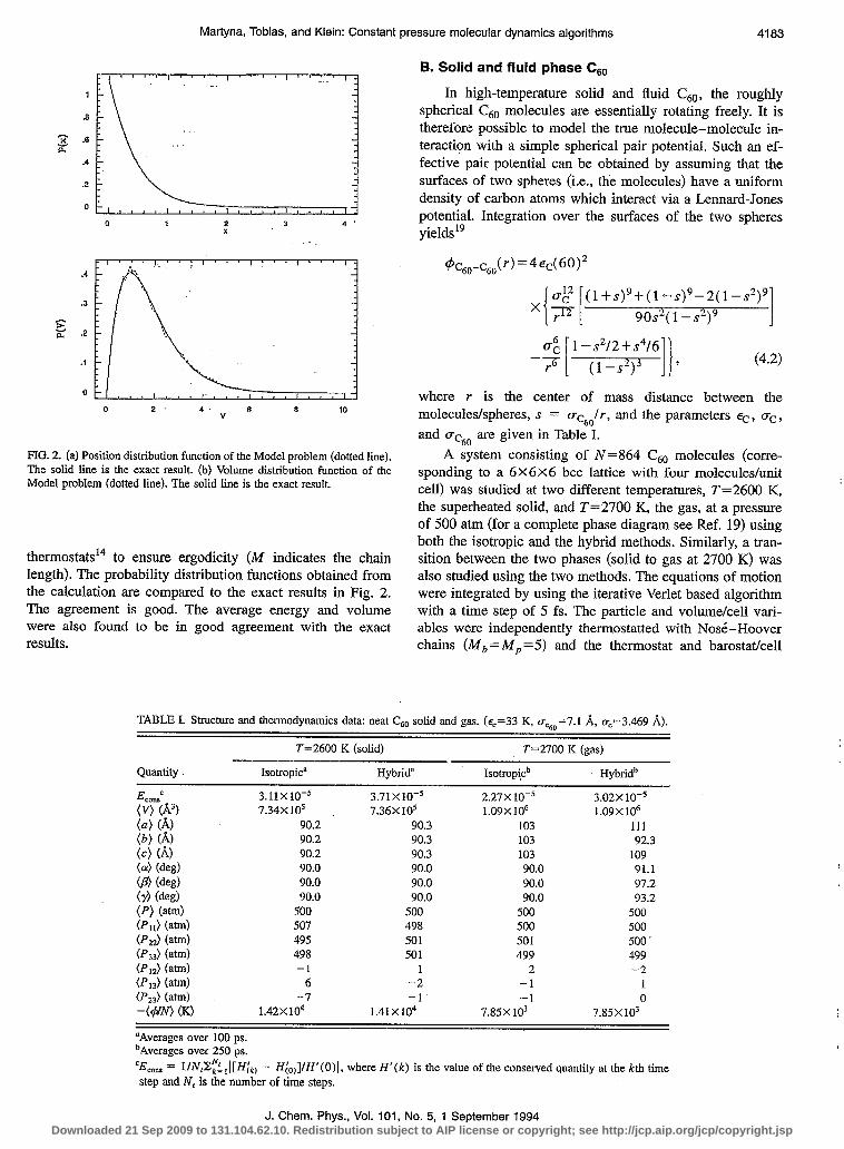
B. Solid and fluid phase CEO

In high-temperature solid and fluid C&,, the roughly spherical C6e molecules are essentially rotating freely. It is therefore possible to model the true molecule-molecule in- teraction with a simple spherical pair potential. Such an effective pair potential can be obtained by assuming that the surfaces of two spheres (i.e., the molecules) have a uniform density of carbon atoms which interact via a Lennard-Jones potential. Integration over the surfaces of the two spheres yields l9

6 Y

0 2 6 10

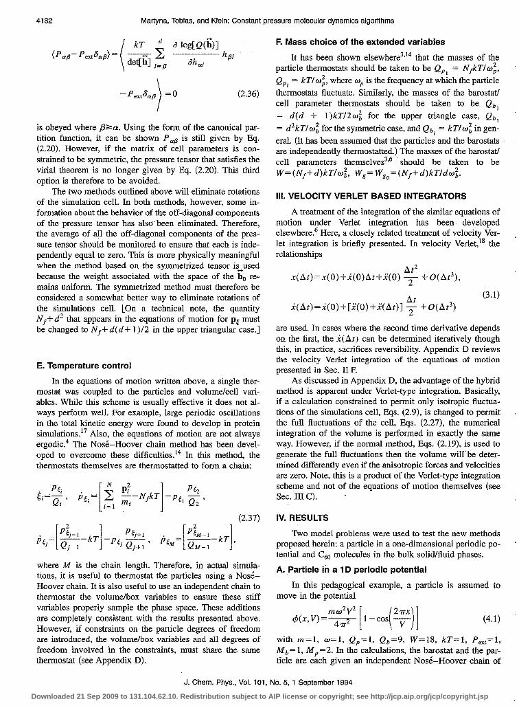
FIG. 2 (a) Position distribution function of the Model problem (dotted line). The solid line is the exact result. (b) Volume distribution function of the Model problem (dotted line). The solid Line is the exact result.

thermostats14 to ensure ergodicity (M indicates the chain length). The probability distribution functions obtained from the calculation are compared to the exact results in Fig. 2. The agreement is good. The average energy and volume were also found to be in good agreement with the exact results.

CT; 1 -s”/2+s4/6 -7 1 I) (l-s”)a ’ (4.2)

where r is the center of mass distance between the molecules/spheres, s = u,-Jr, and the parameters G-., cr,,

and UC,, are given in Table I. A system consisting of N=864 C,, molecules (corre-

sponding to a 6X6X6 bee lattice with four molecules/unit cell) was studied at two different temperatures, T=2600 K, the superheated solid, and T=2700 K, the gas, at a pressure of 500 atm (for a complete phase diagram see Ref. 19) using both the isotropic and the hybrid methods. Similarly, a transition between the two phases (solid to gas at 2700 K) was also studied using the two methods. The equations of motion were integrated by using the iterative Verlet based algorithm with a time step of 5 fs. The particle and volume/cell variables were independently thermostatted with Nose-Hoover chains (M,= M, =5) and the thermostat and barostatkell

TABLE I. Structure and thermodynamics data: neat Cho solid and gas. (+=33 K, 0~~~=7.1 A, o,=3.469 A).

Z-=2600 K(solid) T=2700 K (gas)

Quantity. Isotropic’ Hybrida Isotropicb Hybridb

3.11x10-5 7.34x lo*

90.2 90.2 90.2 90.0 90.0 90.0

ip> (aW 500 Pd Mm) 507 Vu> Wd 495 (p33) (atm) 498 (Pd (ad -1 (p13) W4 6 P23) (aW -7 -MN (K) 1.42x104

3.71x10-5 7.36X10'

90.3 90.3 90.3 90.0 90.0 90.0

500 498 501 501

1

l.41XlliT~

2.27X 10-s 3.02X10+ 1.09x Id 1.09x106

to3 111 103 92.3 103 109 90.0 91.1 90.0 97.2 90.0 93.2

500 500 500 500 501 500. 499 499

2 -2 -1 1 -1 0

7.85X lo3 7.85X103

“Averages over 100 ps. ‘Averages over 250 ps. cJL”, - l/N,Bf&l[H’ (k) - H&JIH’(O)I, where H’(k) is the value of the conserved quantity at the kth time step and N, is the number of time steps.



I”’ I ’ * ’ 1 ” ’ 1 3’ ‘1 “‘1 g2 (4

, , , 1 , , , , , , , , , , , , , , , I-1 0 20 40 60 80 100

time (ps)

I’ a 0 I ” ’ I “‘l ” ’ l’ “I ” (4

1 91

9 90

-I B

i

0 20 40 60 80 100 0 20 40 60 80 100 0 20 40 60 80 100 time (ps) time (ps) me (PSI

3

4

d d

1

8 e

3

8

H ”

93

92

91

90

89

88V 0 20 40 60 80 100

Ume (PSI

93

92

91

90

89

88& 0 20 40 60 80 100

lime (ps)

93

92

91

90

89

g 91 u 5 90 I

89 0 20 40 60 80 100

Ume(~s)

92

j 91

% 90

89 0 20 40 60 80 100

time (ps)

92

-3 8 91

‘: 90

89

FIG. 3. Tiie histories of simulation cell parameters during equilibrium constant NPT simulations of solid CeO at T=2600 K, P,,,=500 atm: (a) isotropic algorithm; (b)-(h) hybrid algorithm.

mass parameters chosen according to the prescription given Equilibrium simulations of the fluid and solid phases are in Sec. II F (q,=2 ps-’ and oP= 1 ps-‘). The potential was considered first. In Figs. 3 and 4, the behavior of the volumes truncated at 40 w and long-range corrections to the potential and individual cell parameters from isotropic and hybrid energy (and the pressure through the Cal) included to ac- simulations of the two state points are compared. In both count for the neglected long-range attractive interactions. phases, the fluctuations of the volume are similar for two

106

3

P 104 5

s

J 102

I

z,

- ,,,I,, , , , , , , , , , , , , , , , , , , , , , , , ,j 0 50 100 150 200 250

lime (ps)

106 ’ I”“,~“‘,~“‘,““,’ (b)

I- i

Ume(ps)

130

(d) 120

110 100

% Qa

90

~

0 50 100 150 200 250

IOO~, , , , , , , , , , , , , , , , , , , , , , , , , ,;1 a . go- 0 50 100 150 200 250 0 50 100 150 200 250

lime (ps) lima (ps)

110

105

100

95

90

85 0 50 100 150 200 250

time (ps)

110 105 100

95

90

85- 0 50 100 150 200 250

time (ps)

110 105

100

95

90

85 0 50 100 150 200 250

the (~9

FIG. 4. Tiie histories of simulation cell parameters during equilibrium constant NPT simulations-of gaseous C6,, at Ti2700 K, P,=500 atm: (a) isotropic algorithm; [b)-(h) hybrid algorithm.




900 0 50 100 150 200 250

time (ps)

110 ' I"",',","","", ('4

900 0 50 100 150 200 250

time (ps)

P 4. e

0 50 100 150 200 250

he (~9

130

120 (d)

110

100

90

80 ~ 0 50 100 150 200 250

lime (ps)

-3 'lo $ too 5 90 I 80

0 50 100 150 200 250

ihe (PSI

120

3 110

c 100

s 90

- :8.,.. 0 50 100 150 200 250

time (ps)

0 50 100 150 200 250 0 50 100 150 200 250 time (ps) time (ps)

E-G. 5. Time histories of simulation cell parameters during constant NPT simulations of a structural transition from solid to gaseous states of C6,, at T=2700 K, I’,,=500 atm: (a] isotropic algorithm; (b)-(h) hybrid algorithm.

methods and in the fully flexible studies (the hybrid calculations) the cell remains essentially cubic on the time scale of the simulations. This second point is by no means guaranteed in the gas phase study where the partition function is independent of cell shape. In fact, cells with large sides (a$,~) and small/large angle2 are a n_on-negligible part of the free shape phase space Jdho G(det[&,]- 1) and will eventually appear. However, the metastability of the roughly cubic cells is a useful result. With the exception of the individual cell lengths and angles in the hybrid gas simulation, the corre- sponding average structural and thermodynamic properties of the two phases computed using the isotropic and hybrid methods are identical within statistical errors (Table I) and agree with previous work at constant volume.“’

The transition from the solid to gas phase was also studied using the two methods (see Fig. 5). Again, the behavior of the volume is similar for the two methods. The transition occurs in roughly 15 ps and the final volumes are the same. In the hybrid study, the cell appears to be distorting slowly, but significantly, from its initially cubic shape. Nonetheless, the transition was not affected and the results are in good agreement with the isotropic calculation.

V. CONCLUSIONS

New constant pressure methodologies have been developed and tested on model and more realistic problems. The methods were found to perform well under equilibrium conditions and during structural transitions such as an evapora- tion of a solid to form a gas. The methods outlined above

should find wide application in modeling condensed phase behavior of complex molecules.

ACKNOWLEDGMENTS

The research described herein was supported by the Na- tional Science Foundation under Grant No. CHE-92-23546. One of us (G. M.) would like to acknowledge startup funds from Indiana University. D. J. T. would like to acknowledge National Institutes of Health Grant No. F32 GM14463.

APPENDIX A

In this appendix, it is shown the conservation law, F cm. =O, can effect the volume distribution function generated by the modified equations of motion, Eqs. (2.7). Basi- cally, satisfying the Liouville equation for the entire distribution is insufficient to guarantee that the individual pieces are properly generated.

In order to demonstrate this important result, consider a system of free particles in a periodic box. The modified equations of motion for the particle positions, the ri, are auxiliary variables, i.e., the dynamics of the ri depend on all the other dynamical variables but not vice versa. Therefore, the time average of any position independent quantity will not depend on the particle positions. The distribution function of the reduced phase space (no positions) is, thus, all important. The reduced phase space (V,p only) generated by the modified equations of motion, Eqs. (2.7), is


-4186 Martyna, Tobias, and Klein: Constant pressure molecular dynamics algorithms

exp[ EIkT] A=(Nf+l)kT s

dpc dp,p dV VNf-l exp

The new equations, Eqs. (2.9), however, generate

exp[ EIKT] N ‘=(Nf+ 1)kT

dpc dp, dp dV V?f exp I 1 -5,

(A3 the isothermal-isobaric/correct result. Basically, the phase space associated with the particle positions serves to mask the fact that the volume distribution produced by Eqs. (2.7) is incorrect.

In the general case, F,.,,=O and ~int=Pint+r~,~..F,.,.,6 the modified equations of motion, Eqs. (2.7), retain the same pathology. In an appropriate set of normal modes, the r,.,. can be seen to be auxiliary variables. This leads to the real- ization that the volume distribution produced by the dynam- its is, in error, by the, now, familiar factor of V, the volume.

APPENDIX B There are two important pressure virial theorems associ-

ated with isothermal-isobaric ensemble that are used in the analysis presented in text. The first and more familiar theorem relates the internal and external pressure

dV wC - PLJI I dp dr D(v)

(pint- pex3 = SdV expC-PPextVIQ(V)[kT{d lodQ(Vl/Jvk pextl =. SdV expII-PP,VlQ(V)

(PinJ=Pext9 @l) while the second and less familiar theorem relates the internal and external work,

((Pint- Pm) v> = SdV wHCJlQWM~T@ W.QW)l~~V~-~extl SdV ew[-PP,,tVIQ(V)

=-kT ,

(PintV> =Pext(V) -kT- 032)

Both theorems are invariant properties of the isothermal- isobaric ensemble and as such are (both) always satisfied, independent of system, boundary condition, etc. (the only input to the derivations is the statistical mechanical definition of the ensemble and the pressure). Incorrect/different ensembles posses incorrect/different virial theorems. For example, the ensemble generated by Hoover dynamics [Eq. (2.1)] has the two theorems

(PinJ=Pext+kT{V-‘),

(PintV>=PexAV~ where the averages are over Eq. (2.5).

033)

(B4)

APPENDIX C

It has been shown elsewhere that for systems with no external forces (X$!= ,Fi=O), the Nod-Hoover canonical dynamics method4’5 only gives rise to the canonical distribution if the total linear momentum is taken to be zero.13 In this appendix, it will be demonstrated that this constraint can be eliminated under No&-.Hoover chain dynamics,‘l a simple extension of the No&-Hoover scheme. In addition, the other “problem” with No&Hoover-type methods under these conditions (XE ,Fi=O), that the total linear momentum can- not change sign or direction is addressed.

The No&-Hoover chain method employs the equations of motion

I

;.=E I Wli ’ $j=-VjV(r)-pj ‘2,

dNslptl . sipr, ~l=-.-.--

QI ) Sj=- Qt ’ (Cl) ’

where each thermostat variable (Si) is in turn thermostatted to form a chain. The dynamics conserves

N 2 M Pi. H’(p,r,s,p&=V(r)+x Pi +c 1 +kT ln(slj

i=l 2% i=l 2Qi M

+ c kT Inisi). G? i=2

However, if 2$ ,ViV(r)=O then P’(t) =P(t)si’dN(t) is also conserved where P(t) = CE lpi(tj is the total linear momentum. The factor of s :IdN appears in this conversation law due to the nonstandard but convenient definition of S, . In general, No&-Hoover dynamics is recovered for M = 1.

J. Chem. Phys., Vol. 101, No. 5,- 1 September 1994


Fist, it will be demonstrated that the Nose-Hoover chain dynamics (M>l), indeed, generates the canonical distribution for the case ZE, Fi =O. The partition function generated by the said dynamics for an ergodic system with the desired constraint Xz ,Fi=O is


values of M, provided the parameter N in Eq. (Al) is de- creased by d. For a more complete treatment of the issues discussed here, see Ref. 24.

APPENDIX D

Q= 1 fi driNfi’ dplfi P,; dsi dP83[s:‘dNP-P’] f-1 i=l i=I i=l

N-l 12 P2 M Pi V(r)+x &--+z+x --f.+kTln(sl)

i=l 2mi i=l 2Qi M

+kTC 1 In(E 3 i-2 1

Q-f fi drtNi’ dp:: p,~~dP Pdel i=l i=l i=l

(C3)

N pi2 p2 M Pi. V(r)+2 -+-+C --!..

i=l 2mi 2~4 i=l 2Qi II ,

where a set of normal modes that separates the total linear momentum {p’,P} but diagonalizes the kinetic energy has been introduced.13 The integrals over the thermostat variables (the s) range from zero to infinity. The canonical ensemble is therefore generated by the dynamics for the for- merly pathological P(O)#O (M>l). (The momentum distribution of the canonical ensemble, by definition, in- cludes the full fluctuations of the center of mass momentum.)

It should be noted that only the magnitude of the total linear momentum P appears in the partition function (Pd-’ exp[-P2/2MkT]). This is consistent with the fact that only the magnitude of the total linear momentum P appears in the equations of motion. Indeed, the total linear momentum can change neither sign nor direction under these conditions due to the structure of the dynamics. Therefore, the center of mass of the system will move off to infinity. This explains why simulations are generally performed with P=O. Nonetheless, the canonical distribution is clearly generated provided Nod-Hoover chains are used as shown above. The directional pathology can be overcome (d > 1) by introducing a matrix of Nose-Hoover chains each coupled to one component of the kinetic energy tensor. (The off- diagonal terms are of course thermostatted to have average value zero not NkT.) Under these conditions, the full fluctuations of the P will be generated.

For completeness, the zero linear momentum condition will be considered. Taking P’(O)=O,sr(O)#O gives P(t)=0 for all time (the fixed point of the dynamics). This is equivalent changing the equation of motion for the particle velocities presented in Eq. (Al) to

(C4)

which can be formally shown to generate canonical ensemble, with the zero linear momentum constraint, for all

In this appendix, velocity Verlet integration of equations of motion that yield the microcanonical ensemble (NVE), the canonical ensemble (NVT) and the isothermal isobaric ensemble (NPT) are reviewed. h

1. Constant energy (AWE)

At constant energy, the velocity Verlet integrator can be applied in a straightforward manner:

r~(At)=ri(O)+vi(O)At+Fi(O) g, i

vi(At)=vi(O)+[F,(O)+Fi(At)] &. (DO

i An arbitrary set of constraints can be handled by the Shake/ Rattle algorithm.‘z22.23

2. Constant temperature (NW)

The velocity Verlet integrator for the equations of motion, Eqs. (2.37), is

ri(Atj=r,(0)+vi(O)At+ F,(O) -------viva mi 1

vi(At)=v,(0)+ Fi(O> --Vi(O>V&O) $

mi 1 1 $,

v~(At)=v~(O~+~G~(O~+G~~~~~l g, where GE=( l/Q)[Xf!=,m,v~--NfkT]. The velocities are in practice determined iteratively through

1

vk,(Atj=v&Oj+[GC(0)+G$Atj] $ (D3j

with initial guess +!(Atj=v&-At)+2G*(O)At. Note, if constraints are present the iterative determination of the velocities is independent of Rattle. That is, Vi(O) +[(Fi(O)lmi)-v~(O)v&Oj+(F~(At)lmJ]Atl;! is Rat- tled and the iterative process is permitted to scale these values. (Rattle enforces ZiVi *V riCj = 0 which is independent of a scaling factor on the v.) This is possible because all par-



titles involved in a common constraint must be coupled to the same thermostat within the present formalism.

3. Constant pressure (NW): Isotropic

In order to integrate Eqs. (2.9), it is convenient to derive velocity Verlet expressions for {q( At) =exp[ - E( At)] Xrj(At),ii(At)=exp[rE(Atj]vi(At)} and then convert them into desired quantities, {r,(At),v&Atj}. The result is

slowly, to provide better temperature control in the simulation.) In addition, Rattle must now be applied as part of the iterative procedure. Alternatively, only the center of mass degrees of freedom of partially rigid or rigid subunits may be barostatted (i.e., scaled by the volume).’ Note that this second procedure produces a slightly different ensemble in partially flexible molecules.

4. Constant pressure (NPT): Flexible

The equations of motion, Eqs. (2.27); the hybrid method, can be integrated by deriving expressions for

,:.

~(Atj=~(O)+v&O)At+G~(O) q, L,

si(Atj=exp[- e(At)]$‘(At)r,(Atj,

ki(At)=exp[-E(Atj]$r(At)vi(At), (W

e(At)=e(O)+v,(O)At+ W)v&O) I

&(At)=?&(At)i;,(At)

from velocity Verlet and then convert them into desired quantities {ri(At).vi(Atj,i;,(Atj]. The result is

-vi(At)v5(At)- vi(At)v,(At) $, 1 v~(At)=vg(0)+[G~(O)+GE(At)] $, -

-I- [

Fi(O) ~~vi(o)v~~o)~2~~o(O~v~(O!

( 2+~)vi~oMo~] 3;.

v,(O)v&O) ; 1 1 At

p-v,(Atjv&Atj T,

where

i

N

Gc=i T mi$+Wv”,-(Nf?l)kT , f-1

I

F,=dV(Pi,t- P& +Gf g mi$.

i 1

~(At)=~[O)+v&O)At+G&O) $;

(D5) -

iD7‘)

The velocities can be determined iteratively as in Sec. D 2 vi(At) =e~~(At)-E(o)ll;o(At)~~ ‘(0) vi(O) + - ,i [

F,(O) ’ ’

and au arbitrary set of constraints on the particle degrees of mi

freedom can be handled using the Shake and Rattle algorithms. However, as the particle velocities are not the time

-V~(0)V~(O)-2~go(O)Vi(O)

derivatives of the particle positions, i=v+vg, all the degrees of freedom involved in the constraints must be coupled to the same thermostat and this thermostat must, in turn, be

-( 2+;)v,(0)v,(0)] $}+[F

coupled to the volume. The volume is partof the surface of -vi(At)vg(At)-2?,,o(Atjvi(At). ‘. constraint and links all the constraints in the problem. (The Lagrange multipliers for all the constraints appear in the volume equations of motion through the pressure tensor and

- i i

2+d Vi( Nf

At)v,(At) g, I

independent sets of constraints can no longer be said to exist as in the NVT case. The restriction on the number of thermostats can be relaxed in the limit that the volume evolves v@t)=v&N+[G&O


I+ G&WI $ ,



At -V,(At)v&At) Y, I-

-T;,o(o)v,(o) ; i;“(O)i-$j ‘(At)

-?&(At)u&&) 1 $ ;

where 1

i

N

GE=; 2 iniV:+~~~-tW~o.Tr[~~o~~o]-(Nf+d”)kT , i=l ; I

Ego= V(Fint-G’& - s Tr[ Fint-YFexJY. 0

038)

The velocities can be determined iteratively a,s in the previous two subsections. The constraint that det[ho]=l must be enforced with a Shake/Rattle routine (see Appendix E). The advantage of the hybrid method over a method involving only h is that the volume is integrated in exactly the same way as in the isotropic case: In addition, the constraint that yso remain symmetric is conserved exactly ,by the integrator (see Sec. II D) and -the angular momenta of the cell remains zero.

APPENDIX E

In this appendix, it is shown ho_w the Shake/Rattle algorithm can be used to constrain det[bJ=l, in the integration of the ~$ybrid method,--Eqs. (2.27). Briefly, if the term -h(det[holL I) is introduced to the conserved quantity-of the hybrid method, Eq. (2.28), then the additional term hI must be added to the force on the Fso in Eqs. (2.27). This results in the term LEO/ Wgo in the expression for zo. In the Shake/ Rattle algorithm’2*23 the following iterative procedure is used to determine the ceil positions at time At and the cell velocities at time A t/2,

.A"&? +b

i&(At)“=i;O(Atjn-’ mtr h,(O), - gn .~

qQ(At/zjrz= ~so(At~2)n-1i;o(Atjn~1 i

(El)

where n labels the iteration number. The value of the nth increment to the total multiplier X” is determined by a first- order Taylor series expansion: ~

- XnAt2* (det[i;o(Atj”-*]-=l j - - =- 2WSO

det[i;o(Atj~-l]Tr[~~l(At)n-~li;o(~Oj~~.':~~~.

032) The iteration proceeds until ]det[&]- ll=O within a desired tolerance. This portion of the algorithm is generally called Shake. The velocity part of the algorithm, Rattle, is trivial since we simply choose the multiplier A so that

t;,,(At)=?sO(Atjo+ (E3)

is traceless:

= -f Tr&JA;jO]. iw

It is important to note that the second time derivatives of all the variables in the problem are velocity dependent. There- fore, the velocities must be generated by repeatedly, (a) iter- ating velocity Verlet itself to convergence and (b) applying Rattle, until all the velocities are determined within a desired tolerance.

The outlined procedures, Shake and iteration plus Rattle, should converge rapidly because the “exact” value of the multiplier has already been substituted into the equations of motion (d Tr[?so]ldt = 0). Thus, only small corrections, on the order of At3, necessary for the finite time step integrator to satisfy the constraint within the.desired tolerance are generated by Shake and Rattle. We therefore find the CPU time taken by this part of the program to be negligible. e

’ H. C. Andersen, J. Chem. Phys. 72, 2384 (1980). *M. Parrinello and A. Rabman, Phys. Rev. Lett. 45, 1196 (1980). “S. Nosd, 3. Chem. Phys. 81, 511,(1984). 4W. G. Hoover, Phys. Rev. A31, 1695 (1985): ‘. ------ ‘.. ‘S. No& and M. L. Klein, Mol. Phys. 50, 1055 (1983). ‘S. Melchionna, G. Ciccotti, and B. L. Holian, Mol. Phys. 78, 533 (1993). 7R. Wentzcqvitch, Phys. Rev. B 44, 2358 (1991). sJ. V. LilJ and J. Q. Broughton, Phys. Rev. B 46, 12;Ofij! (1992). 9W. G; Hoover, Phys. Rev. A 34, 2499 (1486). .’

lo W G. Hoover, in Computational Statistical Mechanics (Elsevier, Amster- dam, 1991)

” M. I? Allen and D. J. Tildesley, Computer Simulation of Liquids @ford University, Oxford, 1989).

“V. I. Arnold, Mathematical Methods of Classical Mechanics (Springer, Berlin, 1978). . . _

13K. Cho. J. D. Joannououlos, and L. Kleinman, Phys,., Rev. B 47, 3145 (1993)...

I

14G. J. Martyr& M. E. Tuckerman, and M. L. Klein, J. Chem. Phys; 97, 2635 (1992): .7 i

“J F Lutsko, in Computer Simulation in Materials Science (Kluwer, Dor- . . drecht, 1991).

‘aJ. R. Ray, J. Chem. Phys. 79, 5128 (1983): 17D. J. Tobias, G. J. Martyna, and M. L. Klein, J. Phys. Chem. 97, 12959

(1993). 18W. C. Swone, H. C. Andersen, P H..Berens, and K. R. Wilson, J. Chem.

Phys. 76, 837 (1982). “L. A. Girifalco, I. Phys. Chem. 96, 858 (1992). “A. Cheng, M. L. Klein, and C. Caccomo, Phys. Rev. Lett. 71, 1200

(1993). ->

z’ M. B. Tuckerman. G. J. Martyna, and B. J, Beme; J. Chem. Phys. 97, 1990 (1992).

‘*J. P. Ryckaert, G. Ciccotti, and H. J. C. Berendsen, J. Comput. Phys. 23, 327 (1977). I- %.

23H. C. Andersen; J. Comput. Phys. 52, 24 (1983). “4G. J. Martyna, Phys. Rev. E (in press)..


constant pressure molecular dynamics algorithms -...

Documents