constant strain triangular element with...

BUILDING RESEARCH JOURNAL

VOLUME 51, 2003 NUMBER 3

CONSTANT STRAIN TRIANGULAR ELEMENTWITH EMBEDDED DISCONTINUITY BASEDON PARTITION OF UNITY

M. AUDY1, J. KRČEK1, M. ŠEJNOHA1*, J. ZEMAN1

The present paper illustrates formulation and implementation of a simple con-stant strain triangle with embedded displacement discontinuity intended for themodeling of localized damage. To arrive at such an element the partition of unityproperty of finite element shape functions is used to introduce the displacementdiscontinuity into the finite element basis. The similarity between standard two di-mensional interface element and the one based on the present formulation is usedto test the behavior of the new element both in bending and tension problems byexamining interfacial tractions developed along a predefined interface with a giveninterfacial stiffnesses. The influence of the selected numerical integration rule is alsoexplored.

Keywords: Partition of unity method, element with embedded discontinuity, con-tact element, interface tractions, elastic energy

1 Introduction

The phenomenological behavior of many engineering materials is characterized by alinear elastic response until their tensile strength is reached followed by the gradual lossof load capacity until failure. Experimentally obtained load-deformation curves exhibita behavior known as a structural softening. The basic mechanisms driving the structuralsoftening are associated with deformation processes taking place on microlevel havinga character of distributed damage (e.g., microcracking) that eventually evolves into alarge discrete failure mode such as cracks. At a certain stage of this process an inelasticdeformation starts to localize in a small area while the rest of a structure tends tounload. This phenomenon is known as strain localization.

Within the finite element framework, the strain-softening (constitutive softening)can be included into the analysis through a suitable choice of material law. Such laws

1 Czech Technical University in Prague, Faculty of Civil Engineering, Department of Struc-tural Mechanics, Thákurova 7, 166 29 Prague 6∗ Corresponding author

1

A. Tesar

are generally phenomenological and contain no actual information about the microscopicbehavior of the material. If no action is taken the combination of finite element contin-uum model and standard rate independent constitutive law enhanced by strain softeningfeatures of the material behavior suffers from inherited mesh dependence. The litera-ture offers a number of ways of solving this problem through a suitable regularizationof constitutive equations such as smeared crack approach, non-local models (Pijaudier-Cabot and Bazant 1987), or gradient regularized models (De Borst and Muhlhaus 1992).The common point of departure of all of these methods is the assumption of smoothcontinuous displacement field throughout a body. From the mechanical point of view,however, the localized failure manifests itself by macroscopical discontinuities that canbe characterized as jumps in the displacement field. Thus introducing a discontinuityinto a kinematic field is a natural way of modeling localized damage. This approach,which takes the name strong discontinuity, has received a considerable attention in theliterature particularly in the last decade ((Moes et al. 1999; Oliver et al. 1999; Oliver etal. 2002; De Proft et al. 2002; Simone et al. 2001; Wells and Sluys et al. 2001), to citea few).

The aim of this paper is to contribute to this field by introducing the most simpleconstant strain triangular element with embedded discontinuity. Apart from standardformulation of governing equations displayed in most of the referenced works this contri-bution also attempts to provide, in an appealing way, a clear guidance for the numericalimplementation of the present element. To identify the basic features of this elementincluding the essential ingredients of its implementation we continue in the footstepsof (Simone et al. 2001) and draw on the formal similarity with the conventional inter-face element to test the behavior of the new element, at present, in the limit of elasticrange.

This paper is organized as follows. The strong discontinuity approach for the deriva-tion of weak governing equations for a body crossed by a discontinuity is pursued inSection 2 to arrive at the constant strain 2-dimensional triangular element with em-bedded displacement discontinuities using the Partition of Unity Method (PUM). Thetheoretical part is completed in Section 3 that provides brief summary of the derivationof 2-dimensional interface element. Several numerical results are presented in Section4. The comparison between PUM-like interface element and the conventional interfaceelement outlined in Section 3 is given including the effect of high interface stiffnesses ontraction oscillations. The contribution concludes by describing the discontinuity fronttracking method, see Section 5.

2 Constant strain triangular element with embedded discontinuity

The present section provides derivation of a simple constant strain triangle enhancedby discontinuous shape functions to allow for jumps in the displacement field (strongdiscontinuity approach). In doing so the partition of unity property of the finite elementshape functions is exploited. Throughout this section, the standard engineering notationis used (see, e.g., (Bittnar and Sejnoha 1996)); the stress and strain tensors written in

2

Constant strain triangular element with embedded discontinuity based on partition of unity

the vector form are given by

σ = σxx σyy σzz σyz σzx σxy T, (1)

and

ε = εxx εyy εzz 2εyz 2εzx 2εxy T. (2)

We further introduce the (3× 6) matrix ∂ defined as

∂ =

∂∂x 0 0 0 ∂

∂z∂∂y

0 ∂∂y 0 ∂

∂z 0 ∂∂x

0 0 ∂∂z

∂∂y

∂∂x 0

, (3)

and the (3× 6) matrix n that stores the components of unit normal vector,

n =

nx 0 0 0 nz ny0 ny 0 nz 0 nx0 0 nz ny nx 0

. (4)

2.1 Kinematics of a displacement jump

Consider a body Ω bounded by a surface Γ and crossed by a discontinuity Γd,Fig 1. Γu represents a portion of Γ with prescribed displacements u while tractions tare prescribed on Γt (Γu∩Γt∩Γd = ∅). The internal discontinuity surface Γd divides thebody into two sub-domains, Ω+ and Ω− (Ω = Ω+∪Ω−). Suppose that the displacementfield can be split into a discontinuous and continuous parts

u(x, t) = u(x, t) +HΓd(x)u(x, t), (5)

where HΓd(x) is the Heaviside function centered at the discontinuity surface Γd (HΓd(x)= 1, ∀x ∈ Ω+ and HΓd(x) = 0, ∀x ∈ Ω−) and u and u are continuous functions onΩ. Note that the discontinuity is introduced by the Heaviside function HΓd(x) at thediscontinuity surface Γd and that the magnitude of the displacement jump [[u]] at thediscontinuity surface is given by u. For small displacements, the strain field assumes theform

ε = ∂Tu =

∂Tu ∀x ∈ Ω−,∂Tu+ ∂Tu ∀x ∈ Ω+ .

(6)

Comparing Eq. (5) with Eq. (6) we finally get

ε = ∂Tu+HΓd∂Tu ∀x ∈ Ω \Γd. (7)

3

A. Tesar

ΩΩ_

+

t

_

Γ

Γ ΓΓ

t

u

dn

ν

Fig. 1. Body Ω crossed by discontinuity Γd

2.2 Kinematics discretization

The displacement field can be interpolated over the body Ω using the concept ofpartition of unity method. For the purpose of this work, it is sufficient to define apartition of unity as a collection of functions ϕi which satisfy (see, e.g, (Babuska andMelenk 1997; Duarte and Oden 1996; Melenk and Babuska et al. 1996) for more details)

n∑i=1

ϕi(x) = 1 ∀x ∈ Ω, (8)

where n is the number of discrete points (nodes). The displacement field will be inter-polated in terms of discrete nodal values by

u(x) =n∑i=1

ϕi(x)

(ai + γi(x)bi

), (9)

where ϕi is a partition of unity function, ai is the discrete nodal value and bi is the’enhanced’ nodal value with respect to ‘enhanced’ basis γi. Note that the standardfinite element shape functions also form a partitions of unity since

n∑i=1

Ni(x) = 1 ∀x ∈ Ω. (10)

4


In the standard finite element method, the partition of unity functions are shape func-tions and the enhanced basis is empty. When adopting the general scheme (9), thediscretized form of the displacement field becomes (Babuska and Melenk 1997; Duarteand Oden 1996; Melenk and Babuska et al. 1996)

u(x) = N(x)a+ N(x)(Nγ(x)b), (11)

where N is a matrix of standard nodal shape functions to interpolate regular nodaldegrees of freedom and vector N(Nγb) serves to introduce certain specific features ofthe displacement field u using the so called enhanced degrees of freedom stored in vectorb. Introduction Eq. (9) into Eq. (16), the strain field is then expressed as

ε(x) = B(x)a+ Bγ(x)b, (12)

where B = ∂TN and Bγ = ∂T(NNγ).A suitable choice of Nγ may considerably improve the description of the displace-

ment field for a specific class of problems (Babuska et al. 2001). When solving, e.g., thelocalized damage problem, the discontinuous displacement field can be easily modeledafter replacing the matrix Nγ by a scalar Heaviside function HΓd multiplied by matrixH (a matrix with entry 1 if the corresponding degree of freedom is enhanced and zerootherwise). Eqs. (11) and (12) then become

u(x) = N(x)a+HΓd(x)N(x)Hb, (13)

ε(x) = B(x)a+HΓd(x)B(x)Hb, (14)

where Eq. (14) holds for x ∈ Ω \Γd.

2.3 Governing equations

Consider a linear elastic body Ω. Assuming small strains and zero body forces, thelinear momentum balance equation and the kinematic equations result in

∂σ = 0, (15)

and

ε = ∂Tu. (16)

The traction and displacement boundary conditions are given by

nσ = t on Γt, (17)

5

A. Tesar

and

u = u onΓu. (18)

The system of governing equations is usually derived by invoking the principle ofvirtual work. In particular, the principle of virtual displacements can be recovered byforcing the equations of equilibrium, Eq. (15), to be satisfied in average sense such that∫

ΩδuT(∂σ) dΩ = 0, (19)

for all statically admissible δu. Splitting the above integral into continuous and discon-tinuous parts we get∫

ΩδuT(∂σ) dΩ +

∫ΩHΓdδu

T(∂σ) dΩ = 0, (20)

for all statically admissible δu and δu. Taking into account the fact that HΓd = 0 on Ω−

we write individual integrals with the help of Green’s theorem, formula for distributionalderivative of the Heaviside function and Eq. (17) as∫

ΩδuT(∂σ) dΩ =

∫ΓtδuTtdΓ−

∫Ω

(∂Tδu

)Tσ dΩ, (21)∫

ΩHΓdδu

T(∂σ) dΩ =∫

ΓtHΓdδu

TtdΓ−∫

Ω

(∂T (HΓdδu

))Tσ dΩ

=∫

Γ+t

δuTt dΓ−∫

ΓdδuTtdΓ−

∫Ω+

(∂Tδu

)Tσ dΩ. (22)

Comparing Eqs. (21) and (22) with Eq. (19) and taking into account the independenceof variations δu and δu we arrive at the weak form of governing equations∫

Ω

(∂Tδu

)Tσ dΩ =

∫ΓtδuTtdΓ, (23)∫

Ω+

(∂Tδu

)Tσ dΩ +

∫ΓdδuTtdΓ =

∫Γ+t

δuTtdΓ. (24)

Finally, inserting the discrete form of Eqs. (13)–(14) into Eqs. (23)–(24) and employingconstitutive equations for the stress σ at a point x ∈ Ω \Γd

σ = Dε = D(Ba+HΓdBb

), (25)

and tractions developed on the discontinuity surface Γd

t = DNb, (26)

6


yields ∫Ω

BTDBadΩ +∫

Ω+BTDBbdΩ =

∫Γt

NTtdΓ, (27)∫Ω+

BTDBadΩ +∫

Ω+BTDBbdΩ +

∫Γd

NTDNbdΓ =∫

Γ+t

NTtdΓ. (28)

The resulting discrete system of linear equations has the traditional form

Ku = f , (29)

where u represents the vector of nodal displacements consisting of standard and en-hanced degrees of freedom

u = a b T, (30)

and f lists externally applied forces

f = fa fb T, (31)

where

fa =∫

ΓtNTtdΓ, (32)

fb =∫

Γ+t

NTtdΓ, (33)

and finally K represents the enhanced stiffness matrix

K =

[Kaa Kab

Kba Kbb

], (34)

where individual sub-matrices are defined as

Kaa =∫

ΩBTDB dΩ, (35)

Kab = KbaT =

∫Ω+

BTDB dΩ, (36)

Kbb =∫

Ω+BTDB dΩ +

∫Γd

NTDN dΓ. (37)

7

A. Tesar

Following the standard finite element procedure, the enhanced stiffness matrix isobtained by the assembly of contribution from individual elements. To that end, thedomain Ω is decomposed into Ne non-intersecting elements Ωe such that Ω = ∪Nee=1Ωe.Formally writing, the global stiffness matrix and the global force vector become

K = ANee=1Ke, (38)

f = ANee=1fe, (39)

where non-zero contributions to enhanced degrees of freedom come either from theelements crossed by the discontinuity,

Kaa,e =∫

ΩeBe

TDeBe dΩ, (40)

Kab,e = Kba,eT =

∫Ω+e

BeTDeBe dΩ, (41)

Kbb,e =∫

Ω+e

BeTDeBe dΩ +

∫Γd,e

NeTDeNe dΓ (42)

or from elements, which are not crossed by a discontinuity but are contained in boththe support of nodal basis function related to an enhanced degree of freedom and theHeaviside function. Then, Ωe+ = Ωe and the contribution from the discontinuity (thesecond term on the right hand side of Eq. (42)) is zero.

2.4 Triangular element

For the 2-dimensional analysis the most simple isoparametric constant strain trian-gular element with linear shape functions, extended by including the enhanced degreesof freedom to enable discontinuity modeling, is derived. The main advantage of a trian-gular family of elements is the possibility of their adapting to virtually any shape andrelative easiness of their implementation. The element is represented by four degrees offreedom in each node. In particular, two standard and two enhanced degrees of freedomserve to describe fully the displacement field within an element. Unlike the original for-mulation, where the displacements were ordered by degrees of freedom, the ordering ofunknowns is now as follows

u = u1 v1 u1 v1 u2 v2 u2 v2 u3 v3 u3 v3 T, (43)

where u and v represent standard displacement degrees of freedom in the x and y

coordinate system, respectively. The corresponding enhanced degrees of freedom are uand v. This ordering displayed in Fig. 2 together with the assumed integration pointsthen allows the use of standard FEM solver. The shape functions for an isoparametric

8


u u~

u~

u

u u~

v~

v v

v~

v

v~

3

21 1 2 2

2

1

11

3 3

3

3

2α

snip1 ip2

ip2ip1

1 2

3

d

d

Fig. 2. Standard and enhanced degrees of freedom for a triangular element and selected Gaussintegration points within the element and on the discontinuity

enhanced triangular element can be defined in terms of area functions as (Bittnar andSejnoha 1996)

N = [L1 L1 L1 L1 L2 L2 L2 L2 L3 L3 L3 L3 ] , (44)

where Li is the function of position (x, y) and element node coordinates xi, yi, i = 1, 2, 3

L1 =a1 + b1x+ c1y

2A

L2 =a2 + b2x+ c2y

2A

L3 =a3 + b3x+ c3y

2A,

where

A =12

∣∣∣∣∣∣1 x1 y11 x2 y21 x3 y3

∣∣∣∣∣∣ (45)

ai = xiyk − xjyi (46)

bi = yj − yk

ci = xk − xj . (47)

9

A. Tesar

The enhanced matrix B can be written as

B(x) =1

2A

[b1 0 b2 0 b3 0 H(x)b1 0 H(x)b2 0 H(x)b3 00 c1 0 c2 0 c3 0 H(x)c1 0 H(x)c2 0 H(x)c3c1 b1 c2 b2 c3 b3 H(x)c1 H(x)b1 H(x)c2 H(x)b2 H(x)c3 H(x)b3

](48)

where H denotes the value of Heaviside function at a point x. Assuming plane stressconditions the material stiffness matrix D is provided by

D =E

1− ν2

1 ν 0ν 1 00 0 2(1 + ν)

. (49)

The (2× 2) discontinuity material stiffness matrix Dlocal given in the local coordinatesystem attains the form

Dlocal =

[Ks 00 Kn

], (50)

where Ks and Kn are the discontinuity stiffnesses in tangential and normal directions,respectively. Using the transformation of coordinates the discontinuity material stiffnessD now written in the global coordinate system becomes

D = TTDlocalT, (51)

where T is the familiar transformation matrix

T =

[cosα sinα− sinα cosα

], (52)

and α represents the angle between the crack alignment and the global x axis.Using the enhanced matrix B, the part of the element stiffness matrix containing

the area integrals, see Eq. (40)–(42), can be written in a compact form as

K1e =

2∑j=1

wiB(ipj)TDB(ipj), (53)

where the integration weights wi are given as areas of triangular and quadrilateralparts of the element (see Section 5 for more detailed discussion). The contributioncorresponding to the discontinuity Γd is computed either by standard two-point Gaussianquadrature or by Newton-Cotes formulae, respectively,

K2bb,e =

2∑j=1

ξjN(ipdj)TDN(ipdj), (54)

10


where ξj and ipdj are the integration weights and points of a selected integration scheme.Finally, the element stiffness matrix assumes the form

Ke =

[K1aa,e K1

ab,e

K1ab,e

T K1bb,e + K2

bb,e

]. (55)

3 Interface element

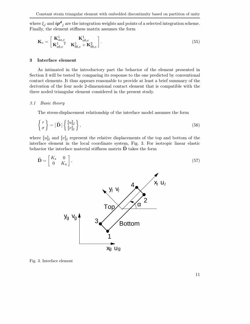
As intimated in the introductory part the behavior of the element presented inSection 3 will be tested by comparing its response to the one predicted by conventionalcontact elements. It thus appears reasonable to provide at least a brief summary of thederivation of the four node 2-dimensional contact element that is compatible with thethree noded triangular element considered in the present study.

3.1 Basic theory

The stress-displacement relationship of the interface model assumes the formτ

σ

= [ D ]

[[u]]l[[v]]l

, (56)

where [[u]]l and [[v]]l represent the relative displacements of the top and bottom of theinterface element in the local coordinate system, Fig. 3. For isotropic linear elasticbehavior the interface material stiffness matrix D takes the form

D =

[Ks 00 Kn

], (57)

uxl ly vl l

x

y v

g

g g

ug

Bottom

Top

1

3

4

2α

Fig. 3. Interface element

11

A. Tesar

where Ks and Kn are in analogy with Eq. (50) the elastic shear and normal stiffnesses,respectively.

3.2 Finite element formulation

In the finite element framework the global displacements are approximated usingthe standard shape functions as

utop = N1u3 +N2u4,

ubot = N1u1 +N2u2,

vtop = N1v3 +N2v4,

vbot = N1v1 +N2v2,

(58)

where the global nodal degrees of freedom ui, vi, now written in the compact form

rg = u1, v1, u2, v2, u3, v3, u4, v4T, (59)

are related to local displacement jumps

[[u]]l[[v]]l

= Brg, (60)

where the matrix B assumes the form

B = [−TB1 −TB2 TB1 TB2] , (61)

and

T =

[cosα sinα− sinα cosα

]Bi =

[Ni 00 Ni

]. (62)

The element stiffness Ke then follows from

Ke =∫ 1

−1BTDBJ dξ, (63)

where J is the element jacobian.

12


4 Example results

In this section we present several example problems that demonstrate the behaviorof both the conventional interface element and element with embedded displacement dis-continuity. The response of the interface element subject to bending loading is examinedfirst. In particular, we focus on the effect of the selected integration rule on the resultinginterface tractions. Similar results are presented for the discontinuous triangular elementand compared to the former one.

Geometry and loading conditions of the selected problems are shown in Figs. 4 and5. As for the material properties we assumed concrete with the Young modulus E equalto 35 MPa and the Poisson ratio ν equal to 0.3.

A B

A B

5m

1m

0.05m

1mF = 20kN

0.2m

Fig. 4. 3-point bending

5m

1m

0.05m

0.2m

AA

2m

F = 10kN F = 10kN

Fig. 5. 5-point bending

13

A. Tesar

-1.5 -1.0 -0.5 0.0 0.5 1.0 1.5stress [MPa]

0.00

0.25

0.50

0.75

1.00

h [m

]

τ : Gauss σ : Gaussτ : Newton-Cotesσ : Newton-Cotesσ : Beam theory

Test: 2D 4-node contact element (elem size 25cm)simple bending: L=5m h=1m b=0.05m (F=20kN at x = 2.5m, section x = 1m)

σ τ

-1.5 -1.0 -0.5 0.0 0.5 1.0 1.5stress [MPa]

0.00

0.25

0.50

0.75

1.00

h [m

]

σ : Beam theory

σ : Newton-Cotesτ : Newton-Cotesσ : Gaussτ : Gauss


στ

-1.5 -1.0 -0.5 0.0 0.5 1.0 1.5stress [MPa]

0.00

0.25

0.50

0.75

1.00

h [m

]

σ : Beam theory



στ

Fig. 6. 3-point bending – Distribution of normal and shear stresses in section A-A, Fig. 4

14


4.1 Conventional interface element

In the first example the attention was given to the distribution of normal and shearstresses in the beam section as a function of the element size. Three different meshes,Fig. 6, were considered. Corresponding results showing the distribution of normal andshear stresses over the beam height developed in section A-A are evident from Fig. 6. Asexpected, refining the finite element mesh considerably improves the predicted responseand both integration schemes give similar results. Fig. 6 also suggests that for coarsermeshes the element formulation based on the Newton-Cotes integration rule providesslightly better results. No significant oscillation of stresses as often reported with theuse of interface elements is evident in this particular example even when relatively highstiffnesses Ks = Kn = 106 GN/m3 were used. The normal stress distribution derivedfrom the beam theory is added for comparison.

Fig. 7. 3-point bending - Finite element mesh used with interface element analysis

As the next example we studied a notch problem. Again, a three-point bending testwas performed. But in this case a notch of length 20 cm was introduced in the structure,see Fig. 4. The finite element mesh used in this example appears in Fig. 7. Both theinfluence of interfacial stiffness and integration rule were examined. Fig. 8.1 clearlyshows the difference between two integration rules, particularly when high stiffness ofthe interface is used. While no oscillation is detected with the Newton-Cotes integrationrule, the Gauss integration scheme results in a significant oscillation of normal stressesin front of the notch tip. The similar conclusion can be drawn from Fig. 8.3. Thiseffect, however, becomes less pronounced when reducing the interfacial stiffness. Also,one may argue that using the Noten-Cotes integration scheme hides on the other handthe true solution by smoothing out the steep gradients when larger elements are used.This effect, however, has not been examined in the present contribution. Thus in view ofFigs. 8.1–8.3 the use of the Newton-Cotes integration rule at least in applications wherean interface element is used to track the displacement discontinuity is preferable. Alsonote a relatively fine mesh used with the present problem, Fig. 7. A slight detour of thestress variation from a straight line at the top of the beam is attributed to the appliedforce placed in the nodes of the interface element.

15

A. Tesar

-8.0 -4.0 0.0 4.0 8.0 12.0 16.0 20.0Normal stress [MPa]

0.0

0.2

0.4

0.6

0.8

1.0h

[m]

Gauss : Kn = 1.0e6 [GN/m3]

Newton-Cotes : Kn = 1.0e6 [GN/m3]

Test: 2D 4-node contact element - notch problem3-point bending L=5m h=1m b=0.05m (E=35GPa F = 20kN at x=2.5m, section 2.5m)


0.0

0.2

0.4

0.6

0.8

1.0

h [m

]

Kn = E/t = 1.0e6 [GN/m3]

Kn = E/t = 1.0e4 [GN/m3]

Kn = E/t = 1.0e2 [GNm3]

2D 4-node contact element with Newton-Cotes integration rule 3-point bending L=5m h=1m b=0.05m (E=35GPa F=20kN at x=2.5m, section x=2.5m)


0.0

0.2

0.4

0.6

0.8

1.0

h [m

]

Kn = E/t = 1.0e6 [GN/m3]

Kn = E/t = 1.0e4 [GN/m3]

Kn = E/t = 1.0e2 [GNm3]

2D 4-node contact element with Gauss integration rule 3-point bending L=5m h=1m b=0.05m (E=35GPa F=20kN at x=2.5m, section x=2.5m)

Fig. 8. 3-point bending – Distribu-tion of normal stress in section B-Bfor notched specimen, Fig. 4

16


4.2 Constant strain triangle with embedded discontinuity

Several example problems are presented in this section to asses the behavior andapplicability of the constant strain triangle enhanced by adding discontinuous shapefunctions. Apart from the apparent application in problems of crack propagation, theformulation of this element presented in Section 3 advocates its possible substitution fora conventional interface element, thus avoiding the need for structured meshes. To eitherconfirm or uproot this suggestion we run a similar set of problems as in the previoussection.

One of the obstacles in using this element is an application of loading along theboundary where enhanced degrees of freedom are activated. In the first set of examplesthis problem was eliminated by loading the beam in four-point bending, Fig. 5, so theforces were applied away from the discontinuity. Also note that closing the discontinuityon the beam edge, setting enhanced degrees of freedom associated with a given elementedge to zero, solves this problem. The effects of closing the discontinuity at the top ofthe beam appears in Fig. 9. While in Fig. 9.1 we force the discontinuity to be closed atthe top of the beam, in Fig. 9.2 the normal displacement jump at that point is free todevelop, which corresponds to reality. Also note almost zero displacement jump in bothcases associated with a relatively high interfacial stiffness.

The corresponding stress distributions are plotted in Fig. 10. An important conclu-sion can be drawn immediately when inspecting Fig. 10. The present enhanced triangu-lar element suffers from oscillation of tractions developed along the discontinuity whenmodeling perfect bond through a high interfacial stiffness. This undesirable feature ap-plies to both integration schemes. On the other hand the stress oscillations completelydisappear when considerably reducing the interfacial stiffness. This situation, however,might not seem to be so critical as even with a relatively low interfacial stiffness onemay arrive at reasonably accurate results. See Fig. 11 showing comparison between theinterface element and the triangular one.

-2e-05 -1e-05 0 1e-05 2e-05Normal strain

0.0

0.2

0.4

0.6

0.8

1.0

h [m

]

Kn = 1e2 [G/m3]

Kn = 1e4 [G/m3]

Kn = 1e6 [G/m3]

PUM like contact element with Newton-Cotes integration rule4-point bending: L=5m h=1m b=0.05m (E=35GPa F=10kN at x=1.5m, section x=2.5m)

Crack tip is closed

Crack is opened

-2e-05 -1e-05 0 1e-05 2e-05Normal strain

0.0

0.2

0.4

0.6

0.8

1.0

h [m

]

Kn = 1e2 [G/m3]

Kn = 1e4 [G/m3]

Kn = 1e6 [G/m3]


Crack tip is opened

Crack is opened

Fig. 9. 4-point bending – Distribution of normal displacement jump in sec. A-A, Fig. 5

17

A. Tesar

-3.0 -2.0 -1.0 0.0 1.0 2.0 3.0Normal stress [MPa]

0.0

0.2

0.4

0.6

0.8

1.0h

[m]

Kn = E/t = 1e6 [GN/m3]

Kn = E/t = 1e4 [GN/m3]

Kn = E/t = 1e2 [GN/m3]


Crack tip is closed

Crack is opened


0.0

0.2

0.4

0.6

0.8

1.0

h [m

]

Kn = E/t = 1e6 [GN/m3]

Kn = E/t = 1e4 [GN/m3]

Kn = E/t = 1e2 [GN/m3]


Crack tip is opened

Crack is opened


0.0

0.2

0.4

0.6

0.8

1.0

h [m

]

Kn = E/t = 1e6 [GN/m3]

Kn = E/t = 1e4 [GN/m3]

Kn = E/t = 1e2 [GN/m3]

Test: PUM like contact element - Gauss integration4-point bending: L=5m h=1m b=0.05m (E=35GPa F=10kN at x=1.5m, section x=2.5m)

Crack tip is closed

Crack is opened


0.0

0.2

0.4

0.6

0.8

1.0

h [m

]

Kn = E/t = 1e6 [GN/m3]

Kn = E/t = 1e4 [GN/m3]

Kn = E/t = 1e2 [GN/m3]

PUM like contact element with Gauss integration rule4-point bending: L=5m h=1m b=0.05m (E=35GPa F=10kN at x=1.5m, section x=2.5m)

Crack tip is opened

Crack is opened

Fig. 10. 4-point bending – Distribution of normal stresses in section A-A, Fig. 5

-2.0 -1.0 0.0 1.0 2.0stress [MPa]

0.00

0.20

0.40

0.60

0.80

1.00

h [m

]

τ : Gauss σ : Gaussτ : Newton-Cotesσ : Newton-Cotesσ : Beam theory

Test: 2D 4-node contact element 4 point bending: L=5m h=1m b=0.05m (F=10kN at x = 1.5m, section x = 2.5m)

στ


0.0

0.2

0.4

0.6

0.8

1.0

h [m

]

Kn = E/t = 1e6 [GN/m3]

Kn = E/t = 1e4 [GN/m3]

Kn = E/t = 1e2 [GN/m3]


Crack tip is opened

Crack is opened

Fig. 11. 4-point bending – Distribution of normal stress in section A-A, Fig. 5

18


Fig. 12. 4-point bending – Finite element mesh and deformation patterns: 1. Kn = 106 [GPa/m3],2. Kn = 104 [GPa/m3], 3. Kn = 102 [GPa/m3]

We now turn our attention to Figs. 10.1 and 10.2. When the enhanced degrees offreedom are constrained (resulting in zero displacement jump) Eq. (26) then predictszero stresses, compare Figs. 9.1 and 10.1. In the present example this is an artificialboundary condition and bears no relevance to the actual deformation of the beam. Onthe other hand, when running a crack propagation analysis, such a condition is generallyapplied at the crack tip to close the crack. This implies that conditions driving the crackanalysis, such as maximum tensile stress, cannot be checked directly at the crack tipbut in elements directly in front of the crack. The finite element mesh used in all aboveexamples together with the deformation pattern for individual interfacial stiffnesses isdisplayed in Fig. 12.

The last set of results is again derived for the three-point bending test. Note thatunlike the normal stresses for which the closed discontinuity is an undesirable condition(normal stress equal to zero on the beam surface) it provides correct results for shearstresses (zero shear on the beam surface). Moreover, Fig. 13 clearly shows the abilityof the enhanced element to represent correctly, at least qualitatively, the singularity

19

A. Tesar

-4.0 -2.0 0.0 2.0 4.0 6.0 8.0 10.0Shear stress [MPa]

0.0

0.2

0.4

0.6

0.8

1.0h

[m]

Ks = 1e2 [GN/m3]

Ks = 1e4 [GN/m3]

Ks = 1e8 [GN/m3]


Crack tip is closed

Crack is opened

-4.0 -2.0 0.0 2.0 4.0 6.0 8.0 10.0Shear stress [MPa]

0.0

0.2

0.4

0.6

0.8

1.0

h [m

]

Ks = 1e2 [GN/m3]

Ks = 1e4 [GN/m3]

Ks = 1e8 [GN/m3]


Crack tip is closed

Crack is opened

Fig. 13. 3-point bending - Distribution of shear stress in section B-B, Fig. 4

-8.0 -6.0 -4.0 -2.0 0.0 2.0 4.0 6.0Normal stress [MPa]

0.0

0.2

0.4

0.6

0.8

1.0

h [m

]

Kn = E/t = 1e2 [GN/m3]

Kn = E/t = 1e4 [GN/m3]

Kn = E/t = 1e6 [GN/m3]


Crack tip is opened

Crack is opened

-8.0 -6.0 -4.0 -2.0 0.0 2.0 4.0 6.0Normal stress [MPa]

0.0

0.2

0.4

0.6

0.8

1.0h

[m]

Kn = E/t = 1e2 [GN/m3]

Kn = E/t = 1e4 [GN/m3]

Kn = E/t = 1e6 [GN/m3]


Crack tip is opened

Crack is opened

-6.0 -4.0 -2.0 0.0 2.0 4.0stress [MPa]

0.00

0.25

0.50

0.75

1.00

h [m

]

σ : Beam theory


Test: 2D 4-node contact element simple bending: L=5m h=1m b=0.05m (F=20kN at x = 2.5m, section x = 2.5m)

στ

Fig. 14. 3-point bending – Distribution of nor-mal stress in section B-B, Fig. 4

of the shear stress under the concentrated load. Note that there was a minor offsetof the point of application of force and the discontinuity end point. Normal stresses

20


-8.0 -4.0 0.0 4.0 8.0 12.0 16.0Normal stress [MPa]

0.0

0.2

0.4

0.6

0.8

1.0h

[m]

Gauss : Kn = 1.0e2 [GN/m3]

Newton-Cotes: Kn = 1.0e2 [GN/m3]

PUM like contact element - notch problem3-point bending: L=5m h=1m b=0.05m (E=35GPa F=20kN at x=2.5m, section x=2.5m)


0.0

0.2

0.4

0.6

0.8

1.0

h [m

]

Kn = E/t = 1e2 [GN/m3]

Kn = E/t = 1e4 [GN/m3]

Kn = E/t = 1e6 [GN/m3]



0.0

0.2

0.4

0.6

0.8

1.0

h [m

]

Kn = E/t = 1e2 [GN/m3]

Kn = E/t = 1e4 [GN/m3]

Kn = E/t = 1e6 [GN/m3]


Fig. 15. 3-point bending – Distribution of nor-mal stress in section B-B for notched specimen,Fig. 4

are plotted in Fig. 14 together with corresponding results derived with the interfaceelement. Similar characteristics of the stress distribution as found for the four-pointbending are recovered. Note that the results displayed in Figs. 14.1 and 14.2 were derivedassuming the nonzero jump condition on both ends of the discontinuity. The results forthe last example, the notch problem, are plotted in Fig. 15. When disregarding thetypical oscillatory response of the enhanced triangular element with the high interfacialstiffness we arrive at the similar distributions of normal stresses in front of the notch asfound with the conventional interface element, recall Fig. 8.

5 Algorithm of crack front tracking

This section briefly outlines the algorithmic aspects and data management for track-ing the two-dimensional crack propagation. We assume that the geometry of the problemis described by a set of nodes, faces and elements and that each face is defined by itsnodes and for each element we are provided with its nodes and faces. Having these dataat our disposal, it appears to be most advantageous to store the crack path with respectto its position on selected faces. The resulting algorithm is then reasonably simple andeasy to implement.

21

A. Tesar

The following notation is extensively used in this section. We denote the set of allnodes in the problem as N , the set of all faces as F and the set of all elements as Ewhile n stands for individual nodes, f for faces and e for elements, respectively. SymbolE(f) is used for the set of all elements sharing a face f , E(n) is used for the set of allelements related to a node n, other sets will be denoted similarly. Further, C(n) denotes(possibly empty) set of all constraints (i.e., supports, prescribed displacements) relatedto a node n and I(e) the set of all element integration points. Symbols ∪= , \= , |=and + = are used in C-language fashion to indicate a given operation with the resultassigned to the left hand side.

5.1 Data initialization

For the sake of completeness, we include a brief description of data initiation for thegiven problem. Function Init extracts information necessary for the analysis of crackpropagation from the set of elements E, i.e., lists of elements related to a node (lines2–3) and elements related to a face (lines 4–5). Finally, it creates the set FC whichcontains all faces crossed by a discontinuity.

Init(E, f0)1 ForEache ∈ E do2 ForEachn ∈ N (e) do3 E(n) ∪= e4 ForEachf ∈ F(e) do5 E(f) ∪= e

6 FC = f0

5.2 Discontinuity insertion

The propagation of crack is driven by inserting strong discontinuities into elementswhich satisfy certain failure criteria. Therefore, CrackElement inserts a crack alignedat a given angle α to a given element ec; f c indicates the last face crossed by the dis-continuity and ε is a certain positive parameter ensuring non-singularity of the elementstiffness matrix (see Section 5). The function returns the element, in which the formationof discontinuity can occur in the next step (line 9).

22


f c

α

xa f =a

y

b

fb

z

f c i

i

1

2

Ω

Ωe+

e−

Fig. 16. Scheme of an enhanced element ec

CrackElement(ec, f c, α, ε,FC)1 ec.tag |= ENHANCED

2 fb = ComputeDiscontinuity(ec, α, fc)3 MarkEnhancedNodes(f c, fb, ε)4 MarkNeighbouringElements(f c, ε)5 SetIntegrationPoints(e, f c, fb)6 RemoveDefaultConstraint(f c)7 AddDefaultConstraint(fb)8 FC ∪= fb9 return(E(fb)\ec)

In the first step (line 1), the element is tagged as ENHANCED* and the next face crossedby the discontinuity is determined (line 2). Then, nodes with enhanced degrees of free-dom (line 3) together with neighboring elements (line 4) are determined. In the nextstep, location and weights of integration points are computed (line 5) and constraintsresulting from prescribe zero values of enhanced degrees of freedom are updated (lines6–7). Finally, the function for the determination of discontinuity position Compute-Discontinuityis presented for the sake of clarity.

* Note that in the real code, this is accompanied by (re)allocation of various informationrelated to the element.

23

A. Tesar

ComputeDiscontinuity(e, α, f c)1 a = GetCrackPos(f c)2 ForEachf ∈ F(e)\f c do3 IfGetIntersection(a, α, f) 6= ∅4 return(f)

5.3 Enhanced degrees of freedom management

Once a new face intersected by a crack (fb) is determined, the nodes on the previouscrack face (fa) should be checked for the sign of the Heaviside function (lines 4–5) andfor the possible enhancement by extended degrees of freedom (lines 6–7).

MarkEnhancedNodes (fa, fb, ε)1 a = GetCrackPos(fa)2 b = GetCrackPos(fb)3 ForEachn ∈ N (fa) do4 If(( ~ab× ~na) · ~e3) > 05 n.tag |= HEAVISIDE

6 IfCheckNodeSupport(n, ε) == TRUE

7 n.tag |= ENHANCED

The support of a basis function related to the nodes tagged as ENHANCED and HEAVISIDE

in the previous procedure then contains elements which are not crossed by a discontinu-ity but are affected by the Heaviside function (see page 6), (lines 2–5). All nodes of suchan element are enhanced by extra degrees of freedom (lines 6–8). Note that the degreesof freedom are not directly linked to the enhanced element and must be constrained tozero value (line 9).

MarkNeighbouringElements(f)1 ForEachn ∈ N (f) do2 If(n.tag == ENHANCED) and(n.tag == HEAVISIDE)3 ForEache ∈ E(n) do4 Ife.tag 6= ENHANCED

5 e.tag |= NEIGHBOR

6 ForEachne ∈ N (e)7 Ifne.tag 6= ENHANCED

8 ne.tag |= ENHANCED

9 C(ne) ∪= DefaultConstraint

The zero values of extended degrees of freedom are enforced by DefaultConstraint,i.e., a constraint which does not affect regular degrees of freedom but fixes values of ex-

24


tended degrees of freedom. Functions RemoveDefaultConstraintand AddDefault-Constraintare used to prescribe zero crack opening on a new crack face (CrackEle-ment , line 7) and to constrain an element basis function for neighboring elements.

RemoveDefaultConstraint(f)1 ForEachn ∈ N (f) do2 C(n) \= DefaultConstraint

AddDefaultConstraint(f)1 ForEachn ∈ N (f) do2 C(n) ∪= DefaultConstraint

5.4 Integration points

In the original work (Wells and Sluys et al. 2001), a relatively complicated 23-pointintegration scheme was used for the numerical evaluation of individual integrals appear-ing in Eqs. (40)–(42). Our approach, however, is substantially simpler as it exploits thelinearity of element basis functions (see Eq. (44)). Thus, the individual terms of elementstiffness matrix remain constant on parts of element Ω+

e and Ω−e (the Heaviside func-tion equal to 1/0) and the corresponding integration weights can be simply obtained asareas of Ω+

e and Ω−e (lines 8–9). The position of integration points is set to the center ofquadrilateral xabz (line 6) and triangle ayb (line 7), respectively. Finally, the sign of theHeaviside function for given integration points is determined in lines 11–12 of functionSetIntegrationPoints .

SetIntegrationPoints(e, fa, fb)1 a = GetCrackPos(fa)2 b = GetCrackPos(fb)3 fc = F(e)\ fa ∪ fb4 x, z = N (fc)5 y = N (e)\x∪ z6 ~i1 = (~a+~b+ ~x+~z)/47 ~i2 = (~a+~b+~y)/38 i2.weight = GetTriangleArea(a, b, y)9 i1.weight = GetTriangleArea(x, y, z)− i1.weight

10 ForEachi ∈ I(e) do11 If((~ia× ~ab) · ~e3) > 012 i.tag |= HEAVISIDE

25

A. Tesar

5.5 Regularity of stiffness matrix

Based on numerical experiments reported in (Wells and Sluys et al. 2001), thesupport of a nodal basis function must fulfill certain conditions to ensure the non-singularity of element stiffness matrix. Specifically, both areas of support of the nodalbasis function with the Heaviside function equal to 1 (area+) or equal to 0 (area−)must be large enough to prevent ill-conditioning of the stiffness matrix (line 12–15 offunction CheckNodeSupportgiven below). In (Wells and Sluys et al. 2001), the valueof ε ≈ 10−4 is suggested.

CheckNodeSupport(n, ε)1 ForEache ∈ E(n) do2 Ife.tag == ENHANCED

3 ForEeachi ∈ I(e) do4 Ifi.tag == HEAVISIDE

5 area++= i.weight

6 Else7 area−+= i.weight

8 ElseIfn.tag == HEAVISIDE

9 area++= GetElementArea(e)10 Else11 area−+= GetElementArea(e)12 If min(area+, area−) < ε(area+ + area−)13 return(FALSE)14 Else15 return(TRUE)

6 Conclusion

The derivation of a simple constant strain triangle with embedded discontinuity waspresented. Number of examples were analyzed to test the behavior of the element. In par-ticular, the three-point and four-point bending tests were selected in the present study.The element was tested in view of its ability to replace a conventional interface elementand thus avoid the need for structured meshes. To that end, normal and shear stressesdeveloped along a predefined discontinuity, recall Figs. 4 and 5, were plotted. The finaldistributions were compared with the similar results provided by the interface element.Unlike the interface element, the present triangular element suffers from significant os-cillations of discontinuity tractions, particularly when the the initially elastic behaviorwith zero discontinuity jumps is represented. This unwanted behavior is attributed toinitially high interface stiffness (correct representation of elastic “undamaged” responsecorresponds to infinite interface stiffness). This undesirable effect is not satisfactorilysolved when using the Newton-Cotes integration scheme in place of the more standard

26


Gauss integration scheme. On the other hand, when allowing for a certain “small” dis-placement jump along the discontinuity by reducing the interface stiffness the correctrepresentation of interfacial tractions, normal and shear stresses in the present exampleproblems, is recovered. This property is appealing and it might be expected that theenhanced element will perform well in applications where reduction of stiffness due todamage (cracks, shear bends) is expected. This will be the subject of the future work.

Acknowledgements. We would like to express our thanks to K. deProft and A. Simone fornumerous interesting discussions and suggestions. Financial support for this project was providedby the GACR 106/02/0678 grant.

REFERENCES

[1] BABUSKA, I., BANERJEE, U., and OSBORN, J. E. (2001), “On Principles for the Selectionof Shape Functions for the Generalized Finite Element Method.” Report No. 01-16 TICAM.

[2] BABUSKA, I. and MELENK, J. M. (1997), “The Partition of Unity Method.” InternationalJournal for Numerical Methods in Engineering 40, 727–758.

[3] BITTNAR, Z. and SEJNOHA, J. (1996), “Numerical methods in structural engineering.”ASCE Press.

[4] DE BORST, R. and MUHLHAUS, H. B. (1992), “Gradient dependent plasticity – formula-tion and algorithmic aspects.” International Journal for Numerical Methods in Engineering35, 521–539.

[5] DE PROFT, K., DE WILDE, W. P., Sluys, L. J. (2002), “A combined damage-plasticitymodel for discontinuous modeling of fracture.” Proceedings of the Fifth World Congress onComputational Mechanics (WCCM V), Mang, H. A., Rammerstorfer, F. G. and Eberhard-steiner, J., eds. Vienna University of Technology.

[6] DUARTE, C. A. and ODEN, J. T. (1996), “H-p clouds and h-p meshless method.” NumericalMethods for Partial Differential Equations 12, 521–539.

[7] MELENK, J. M. and BABUSKA, I. (1996), “The Partition of Unity Finite Element Method:Basic Theory and Applications.” Computer Methods in Applied Mechanics and Engineering139, 298–314.

[8] MOES, N., DOLBOW, J. and BELYTSCHKO, T. (1999), “A finite element method for crackgrowth without remeshing.” International Journal for Numerical Methods in Engineering 46,131–151.

[9] OLIVER, J., CERVERA, M., MANZOLI, O. (1999), “Strong discontinuities and continuumplasticity models: The strong discontinuity approach.” International Journal of Plasticity15, 131–151.

[10] OLIVER, J., HUESPE, A. E., PULIDO, M. D. G, and CHAVES, E. (2002), “From con-tinuum mechanics to fracture mechanics: the strong discontinuity approach.” EngineeringFracture Mechanics 69, 131–151.

[11] PIJAUDIER-CABOT, G. and BAZANT, Z. P. (1987), “Non local damage theory.” ASCEJournal of Engineering Mechanics 113, 1512–1533.

[12] SIMONE, A., REMMERS, J. J. C. and WELLS, G. N. (2001), “An interface element basedon the partition of unity.” Report No. CM2001.007, TU Delft.

[13] WELLS, G. N. and SLUYS, L. J. (2001), “A new method for modelling cohesive cracks.”International Journal for Numerical Methods in Engineering 50, 2667–2682.

27

constant strain triangular element with...

Documents