constitutive models for geotechnical practice...constitutive models for geotechnical practice rafal...
TRANSCRIPT
Constitutive models for geotechnical practice
in ZSoil v2016
Rafal OBRZUD
ZSoil® August 2016
1

Constitutive models for geotechnical practice
Rafal Obrzud
22.08.2015, Lausanne, Switzerland
Introduction
Initial stress state and definition of effective stresses
Saturated and partially-saturated two-phase continuum
Introduction to the Hardening Soil model (HSM)
Undrained behavior analysis using HSM
Practical applications of HSM
Assistance in parameter identification
Contents
2

Constitutive models for geotechnical practice
Rafal Obrzud
22.08.2015, Lausanne, Switzerland
Constitutive laws for finite element analysis
Goal of FE analysis:
reproduce as precisely as possible stress-strain response of a
system subject to different or complex stress paths
3

Constitutive models for geotechnical practice
Rafal Obrzud
22.08.2015, Lausanne, Switzerland
Continuum models available in ZSoil v2014
Basic laws
Advanced laws
(more or less complex)
01
2
3
4

Constitutive models for geotechnical practice
Rafal Obrzud
22.08.2015, Lausanne, Switzerland
Better approximation of soil behavior for simulations of practical cases
Plasticity (yielding) before reaching the ultimate state
Why do we need advanced constitutive models?
q = s1-s3
s3
5
Stress path
3
2' 31 ss p
qTriaxial stress conditions
(e.g. under footing)

Constitutive models for geotechnical practice
Rafal Obrzud
22.08.2015, Lausanne, Switzerland
Why do we need advanced constitutive models?
Accounting for stress history and volumetric plastic straining
6
sv
error …
Odometer test conditions
(e.g. very wide foundation)
'p
q

Constitutive models for geotechnical practice
Rafal Obrzud
22.08.2015, Lausanne, Switzerland
ENGINEERING CALCULATIONS
ULTIMATE STATE ANALYSIS
Bearing capacity
Slope stability
DEFORMATION ANALYSIS
Pile, retaining wall deflection
Supported deep excavations
Tunnel excavations
Consolidation problems
Basic models e.g. Mohr-Coulomb Advanced soil models
Why do we need advanced constitutive models?
7

Constitutive models for geotechnical practice
Rafal Obrzud
22.08.2015, Lausanne, Switzerland
Mohr-Coulomb
p’
q
K0-line
yield
surface
Linear
elastic
domain
e1
q
E Eur
E = Eur
p’
q
K0-
unloading
Basic differences between implemented soil models
8

Constitutive models for geotechnical practice
Rafal Obrzud
22.08.2015, Lausanne, Switzerland
Tunneling
Standard Mohr-Coulomb Hardening-Soil
Practical applications of the Hardening Soil model
9

Constitutive models for geotechnical practice
Rafal Obrzud
22.08.2015, Lausanne, Switzerland
Mohr-CoulombVolumetric cap
models
p’
q
K0-line
yield
surface
p’
q
e1
q
E Eur
e1
q
Eur
E=Eur
Stiffness
degradation
isotropic
hardening
mechanism
E
E < Eur
p’
q
s1’ constant
Linear
elastic
domain
Linear
elastic
domain
Basic differences between implemented soil models
10
Constitutive models for geotechnical practice
Rafal Obrzud
22.08.2015, Lausanne, Switzerland
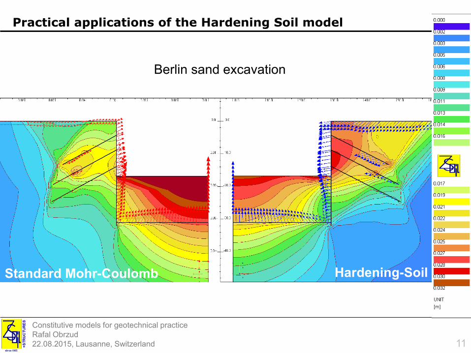
Standard Mohr-Coulomb Hardening-Soil
Berlin sand excavation
Practical applications of the Hardening Soil model
11

Constitutive models for geotechnical practice
Rafal Obrzud
22.08.2015, Lausanne, Switzerland
Mohr-CoulombVolumetric cap
modelsHardening Soil
models
p’
q
K0-line
yield
surface
Linear
elastic
domain
p’
q
p’
q
e1
q
E Eur
e1
q
Eur
e1
q
Eur
E0
E=Eur
Stiffness
degradation
Stiffness
degradation
isotropic
hardening
mechanism+ shear
hardening
mechanism
E
E<EurEur
Linear
elastic
domain
E0
E
NON-LINEAR elastic domain
Basic differences between implemented soil models
12

Constitutive models for geotechnical practice
Rafal Obrzud
22.08.2015, Lausanne, Switzerland
Introduction
Initial stress state and definition of effective stresses
Saturated and partially-saturated two-phase continuum
Introduction to the Hardening Soil model (HSM)
Undrained behavior analysis using HSM
Practical applications of HSM
Assistance in parameter identification
Contents
13

Constitutive models for geotechnical practice
Rafal Obrzud
22.08.2015, Lausanne, Switzerland
Defining type of analysis
14

Constitutive models for geotechnical practice
Rafal Obrzud
22.08.2015, Lausanne, Switzerland
Setting parameters: Initial state setup
15
Constitutive models for geotechnical practice
Rafal Obrzud
22.08.2015, Lausanne, Switzerland
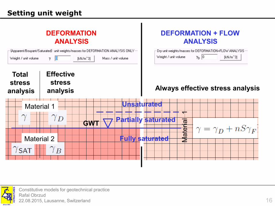
Setting unit weight
DEFORMATION
ANALYSIS
DEFORMATION + FLOW
ANALYSIS
GWTPartially saturated
Unsaturated
Fully saturated
Total
stress
analysis
Effective
stress
analysis Always effective stress analysis
Material 1
Material 2 Mate
rial 1
16

Constitutive models for geotechnical practice
Rafal Obrzud
22.08.2015, Lausanne, Switzerland
Imposing initial stresses using superelements
NB. Effective initial stresses setup is mandatory for Modified Cam-clay
s'YY h D F n0 1-
s'XX K0 s'YY
s'ZZ s'XX
Below GWT
´ sat F-Below GWT
17

Constitutive models for geotechnical practice
Rafal Obrzud
22.08.2015, Lausanne, Switzerland
Introduction
Initial stress state and definition of effective stresses
Saturated and partially-saturated two-phase continuum
Introduction to the Hardening Soil model (HSM)
Undrained behavior analysis using HSM
Practical applications of HSM
Assistance in parameter identification
Contents
18

Constitutive models for geotechnical practice
Rafal Obrzud
22.08.2015, Lausanne, Switzerland
Od nienasyconego do pełnego stanu nasycenia gruntu
19
from Nuth (2009)
S - saturation degree
pw – pressure in liquid phase
NB. fluid = liquid + gas
Interstitial pressureSaturation degree
+
-
p>0
p<0

Constitutive models for geotechnical practice
Rafal Obrzud
22.08.2015, Lausanne, Switzerland
Effective stress in ZSoil
20
Bishop’s effective stress in single-phase model for fluid
Fluid is considered as a mixture of air and water (single-phase model of fluid)
p – pore water pressure
S = S(p) – degree of saturation depending on pore water pressure
suction stressif p > 0 (above GWT)
Constitutive models for geotechnical practice
Rafal Obrzud
22.08.2015, Lausanne, Switzerland
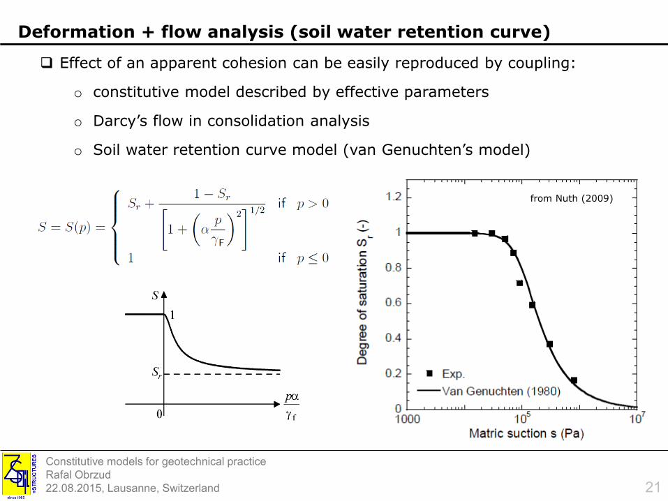
Deformation + flow analysis (soil water retention curve)
Effect of an apparent cohesion can be easily reproduced by coupling:
o constitutive model described by effective parameters
o Darcy’s flow in consolidation analysis
o Soil water retention curve model (van Genuchten’s model)
from Nuth (2009)
21

Constitutive models for geotechnical practice
Rafal Obrzud
22.08.2015, Lausanne, Switzerland
Effective stress principle
Bishop stress
All constitutive models are formulated in terms of effective stresses
Therefore effective stress parameters should be used
o Effective stiffness parameters E′, E′0, E′ur, E′50, n′, n′ur
o Effective strength parameters f′, c′
Deformation + flow analysis (uncoupled or coupled)
22
Constitutive models for geotechnical practice
Rafal Obrzud
22.08.2015, Lausanne, Switzerland
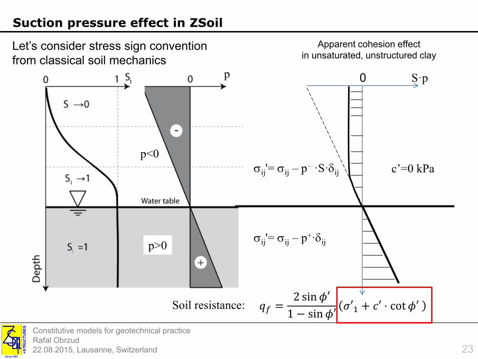
Suction pressure effect in ZSoil
23
0 S·p
c’=0 kPa
Apparent cohesion effect
in unsaturated, unstructured clay
p
p<0
p>0sij'= sij – p+·dij
Let’s consider stress sign convention
from classical soil mechanics
sij'= sij – p– ·S·dij
𝑞𝑓 =2 sin𝜙′
1 − sin𝜙′𝜎′1 + 𝑐′ ⋅ cot 𝜙′Soil resistance:
Constitutive models for geotechnical practice
Rafal Obrzud
22.08.2015, Lausanne, Switzerland
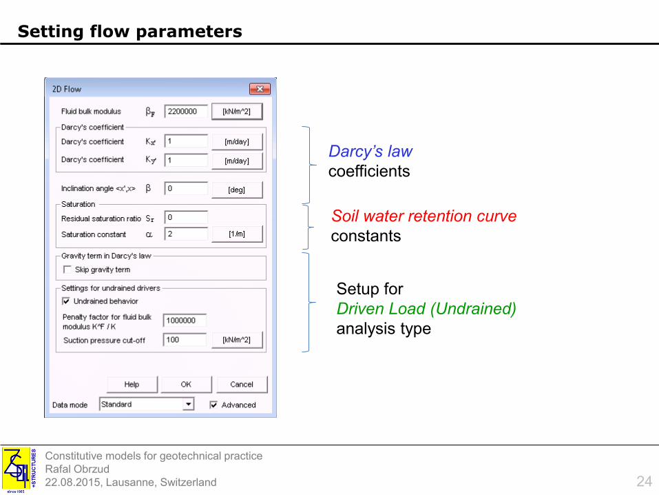
Setting flow parameters
Darcy’s law
coefficients
Soil water retention curve
constants
Setup for
Driven Load (Undrained)
analysis type
24

Constitutive models for geotechnical practice
Rafal Obrzud
22.08.2015, Lausanne, Switzerland
Setting flow parameters
from Nuth (2009)
Flow parameters from Yang & al. (2004)
Soil type a [1/m] Sr [-]
Gravely Sand
100 0
Medium Sand
10 0
Fine Sand 8 0
Clayey Sand
1-1.7 0.09-0.23
Fines content , constant a
25
a can be taken as an inverse of height
of the capillary rise

Constitutive models for geotechnical practice
Rafal Obrzud
22.08.2015, Lausanne, Switzerland
Setting flow parameters
26
Saturation constant taken as the inverse of the capillary rise
Soil type a [1/m]
Silt 0.2 – 0.5
Clay: low plasticity (lean clay) 0.2 – 0.5
Clay: medium plasticity 0.083 – 0.25
Clay: high plasticity (fat clay) 0.125 – 0.05
Clay: very high plasticity 0.033 – 0.067

Constitutive models for geotechnical practice
Rafal Obrzud
22.08.2015, Lausanne, Switzerland
Effect of SWRC constants on soil strength
Reproducing an apparent cohesion
o Effective stress principle (Bishop)
o Find a limit for S·p (for p ) using van Genuchten’s model
o For Sr = 0.0 and p
a
FpS
Suction(apparent cohesion)
Positive pore pressure above GWT
27

Constitutive models for geotechnical practice
Rafal Obrzud
22.08.2015, Lausanne, Switzerland
Effect of SWRC constants on soil strength
Reproducing an apparent cohesion
o For Sr > 0.0 and p S·p (for p )
Suction(apparentcohesion)
Positive pore pressure above GWT
NB.To avoid too much apparent cohesion above the GWT set Sr = 0.0 and an
appropriate a value(e.g. if a 1.0, the apparent
cohesion will not exceed 10 kPa)
28

Constitutive models for geotechnical practice
Rafal Obrzud
22.08.2015, Lausanne, Switzerland
Effect of SWRC constants on soil strength
29
Max suction S·p = 13 kPa
Single phase (Deformation): Instability at initial state analysis
Two-phase (Deformation+Flow): Stability at initial state analysis
f =30°
c = 0 kPa
a=45°

Constitutive models for geotechnical practice
Rafal Obrzud
22.08.2015, Lausanne, Switzerland
Effect of SWRC constants on soil strength
30
Max suction S·p = 8 kPa
Heavy rain bydistributed fluxes
Instability

Constitutive models for geotechnical practice
Rafal Obrzud
22.08.2015, Lausanne, Switzerland
Effect of SWRC constants on soil strength
31
Excavation
Steady-state analysis Consolidation

Constitutive models for geotechnical practice
Rafal Obrzud
22.08.2015, Lausanne, Switzerland
Exercise 1 – Determining the initial state
32
Medium sand Clayey sand Clay
D (SAT)[kN/m3] 16.5 (20.3) 17.6 (21.4) 16.5 (20.9)
e0 [-] 0.6 0.6 0.8
a [1/m] 10 1.0 0.25
Open file:Ex_1_InitialState.inp
-10.00
0.00
-20.00

Constitutive models for geotechnical practice
Rafal Obrzud
22.08.2015, Lausanne, Switzerland
Exercise 1 – Determining the initial state
33
Defining physical properties and hydraulic constants

Constitutive models for geotechnical practice
Rafal Obrzud
22.08.2015, Lausanne, Switzerland
Exercise 1 – Determining the initial state
34
Problem type:
Deformation+Flow
Analysis type:
Initial State

Constitutive models for geotechnical practice
Rafal Obrzud
22.08.2015, Lausanne, Switzerland
Exercise 1 – Determining the initial state
35
Import sections Ex_1_Sections.sec
Profiles of saturation degree

Constitutive models for geotechnical practice
Rafal Obrzud
22.08.2015, Lausanne, Switzerland
Exercise 1 – Determining the initial state
36
S*p profiles

Constitutive models for geotechnical practice
Rafal Obrzud
22.08.2015, Lausanne, Switzerland
Introduction
Initial stress state and definition of effective stresses
Saturated and partially-saturated two-phase continuum
Introduction to the Hardening Soil model (HSM)
Undrained behavior analysis using HSM
Practical applications of HSM
Assistance in parameter identification
Contents
37
Constitutive models for geotechnical practice
Rafal Obrzud
22.08.2015, Lausanne, Switzerland
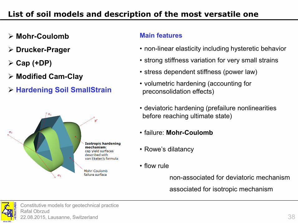
List of soil models and description of the most versatile one
Mohr-Coulomb
Drucker-Prager
Cap (+DP)
Modified Cam-Clay
Hardening Soil SmallStrain
Main features
• non-linear elasticity including hysteretic behavior
• strong stiffness variation for very small strains
• stress dependent stiffness (power law)
• volumetric hardening (accounting for
preconsolidation effects)
• deviatoric hardening (prefailure nonlinearities
before reaching ultimate state)
• failure: Mohr-Coulomb
• Rowe’s dilatancy
• flow rule
non-associated for deviatoric mechanism
associated for isotropic mechanism
38
Constitutive models for geotechnical practice
Rafal Obrzud
22.08.2015, Lausanne, Switzerland
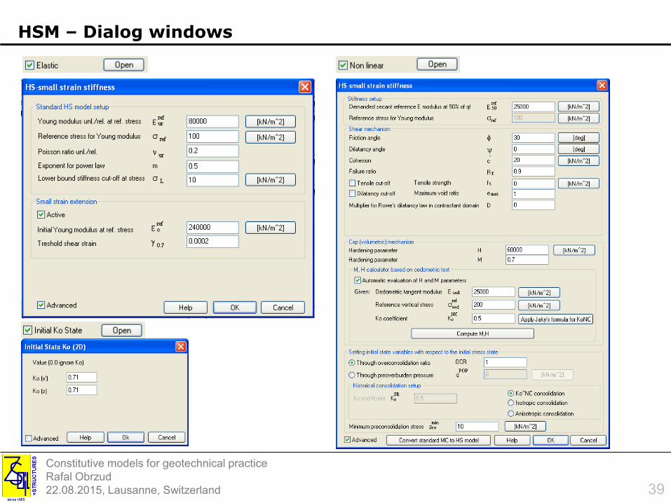
HSM – Dialog windows
39

Constitutive models for geotechnical practice
Rafal Obrzud
22.08.2015, Lausanne, Switzerland
Small strain stiffness in geotechnical practice
Strain range in
which soils can be
considered truly
elastic is very small
Once a certain
shear strain
threshold is reached
a strong stiffness
degradation is
observed
On exceeding the
domain of non-linear
elasticity, plastic
(irreversible) strains
develop
40

Constitutive models for geotechnical practice
Rafal Obrzud
22.08.2015, Lausanne, Switzerland
Hardening Soil model framework
41
Constitutive models for geotechnical practice
Rafal Obrzud
22.08.2015, Lausanne, Switzerland
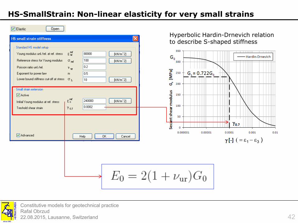
Hyperbolic Hardin-Drnevich relation to describe S-shaped stiffness
HS-SmallStrain: Non-linear elasticity for very small strains
e1 - e3 )
42

Constitutive models for geotechnical practice
Rafal Obrzud
22.08.2015, Lausanne, Switzerland
Determination of G0 from geophysical tests, SCPT, SDMT and others
with r denoting density of soil and Vs shear wave velocity. (n=0.15..0.25 for small strains)
In situ tests with seismic sensors:
• seismic piezocone testing (SCPTU)
(Campanella et al. 1986)
• seismic flat dilatometer test (SDMT)
(Mlynarek et al. 2006, Marchetti et al. 2008)
• cross hole, down hole seismic tests
Geophysical tests: (see review by Long 2008)
• continuous surface waves (CSW)
• spectral analysis of surface waves (SASW)
• multi channel analysis of surface waves (MASW)
• frequency wave number (f-k) spectrum method
HS-SmallStrain: Non-linear elasticity– estimation of E0
43

Constitutive models for geotechnical practice
Rafal Obrzud
22.08.2015, Lausanne, Switzerland
HS-SmallStrain: Non-linear elasticity– estimation of Vs from SPT
For correlations see report on HS model in Zsoil Help
44
𝐺0 = 𝜌 ⋅ 𝑉𝑠2
Vs measured at given depth at s’v0
𝐺0 = 𝐺0(𝜎′3)
where:
𝜎′3 = 𝑚𝑖𝑛 (𝜎′
𝑣0 ⋅ 𝐾0, 𝜎′𝑣0)
then 𝐺0 can be scaled to 𝜎𝑟𝑒𝑓 :
(correlations for all types of soil)
𝐺0𝑟𝑒𝑓
(𝜎𝑟𝑒𝑓) =𝐺0(𝜎
′3)
𝜎′3 + 𝑎
𝜎𝑟𝑒𝑓 + 𝑎
𝑚
with : 𝑎 = 𝑐′ ⋅ cot 𝜙′
Constitutive models for geotechnical practice
Rafal Obrzud
22.08.2015, Lausanne, Switzerland
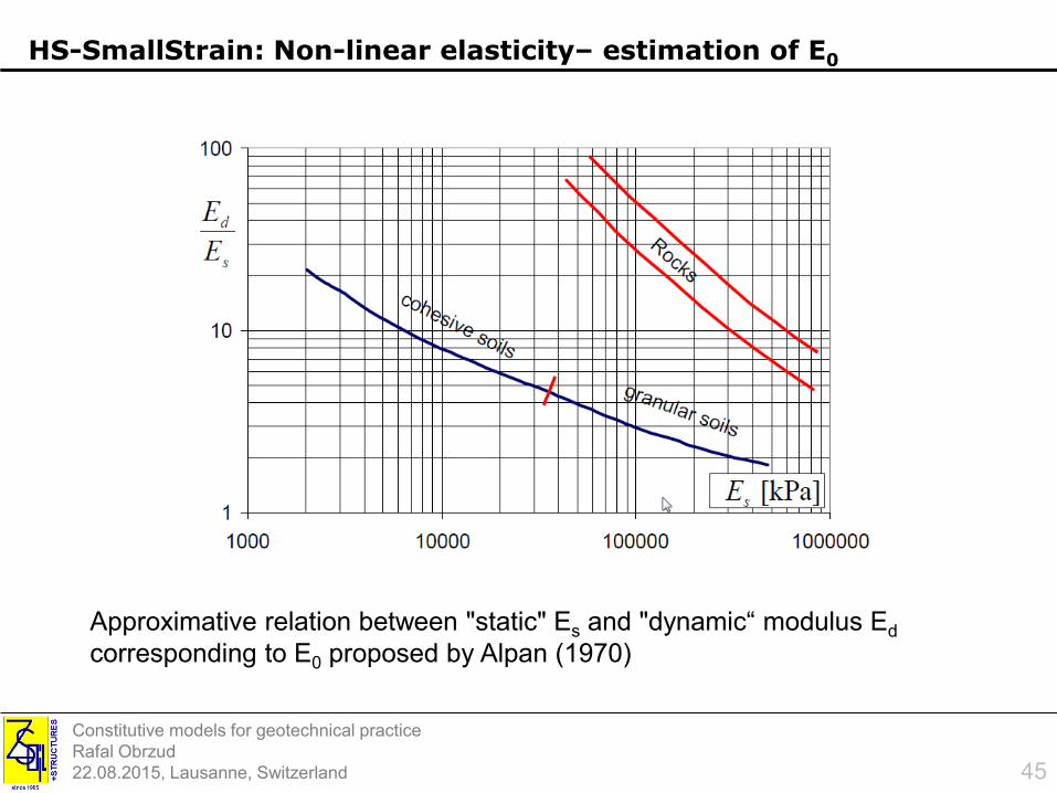
HS-SmallStrain: Non-linear elasticity– estimation of E0
45
Approximative relation between "static" Es and "dynamic“ modulus Ed
corresponding to E0 proposed by Alpan (1970)
Constitutive models for geotechnical practice
Rafal Obrzud
22.08.2015, Lausanne, Switzerland
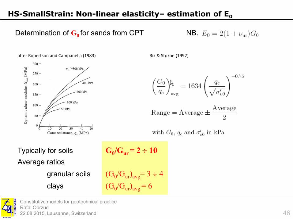
after Robertson and Campanella (1983)
Determination of G0 for sands from CPT
HS-SmallStrain: Non-linear elasticity– estimation of E0
Rix & Stokoe (1992)
Typically for soils G0/Gur = 2 10
Average ratios
granular soils (G0/Gur)avg= 3 4
clays (G0/Gur)avg = 6
NB.
46

Constitutive models for geotechnical practice
Rafal Obrzud
22.08.2015, Lausanne, Switzerland
Relation between E0 and E50
HS-SmallStrain: Non-linear elasticity– estimation of E0
Natural clays
E0 / E50 = 5 30higher values for the ratio are
suggested for aged, cemented and
structured clays, whereas the lower
ones for insensitive, unstructured and
remoulded clays
Granular soils
E0 / E50 = 4 18higher values are suggested for
normally-consolidated soils
See HS Report
47

Constitutive models for geotechnical practice
Rafal Obrzud
22.08.2015, Lausanne, Switzerland
after Wichtmann & Triantafyllidis (2004)
Granular soils 0.7 mainly depends on magnitude of mean eff. stress p’
Typically for clean sands and pref = 100kPa:
810-5 < 0.7 < 2 10-4
HS-SmallStrain: Non-linear elasticity at small strains
For more correlations see report on HS model in Zsoil Help
48

Constitutive models for geotechnical practice
Rafal Obrzud
22.08.2015, Lausanne, Switzerland
Cohesive soils
Influence of soil plasticity
after Vucetic&Dobry (1991) Stokoe et al. 2004
0.7 depends on soil plasticity PI, wL, , wP
HS-SmallStrain: Non-linear elasticity for small strains
For more correlations see report on HS model in Zsoil Help
49

Constitutive models for geotechnical practice
Rafal Obrzud
22.08.2015, Lausanne, Switzerland
Hardening Soil: Double hardening model
Why do we need two hardening mechanisms?
1. Volumetric plastic strains are often dominant in normally consolidated
clays and loose sands
2. Deviatoric (shear) plastic strains are dominant in overconsolidated and
dense sands
3. In practice, all depends on stress paths …
50

Constitutive models for geotechnical practice
Rafal Obrzud
22.08.2015, Lausanne, Switzerland
Hardening Soil: Double hardening – shear hardening
Pure deviatoric shear in overconsolidated material with HS Standard model
s0 Initial stress state
s0 -sp Linear elastic
sp -sf Elasto-plastic
sf On failure surface
sf -su Linear elastic
q = s1-s3
51

Constitutive models for geotechnical practice
Rafal Obrzud
22.08.2015, Lausanne, Switzerland
E50 – secant stiffness modulus corresponding to 50% of the ultimate
deviatoric stress qf described by Mohr-Coulomb criterion
Eur – unloading/reloading modulus
For most soils Rf falls between 0.75 and 1
Hardening Soil: Hyperbolic approximation of the stress-strain
hardening parameter which tracks the evolution of the deviatoric mechanism that evolves with the deviatoricplastic strains
52

Constitutive models for geotechnical practice
Rafal Obrzud
22.08.2015, Lausanne, Switzerland
Hardening Soil: Stiffness moduli
Typically for most soils:
Eur / E50 = 2 ÷ 6
Must be satisfied: Eur / E50 >2
53

Constitutive models for geotechnical practice
Rafal Obrzud
22.08.2015, Lausanne, Switzerland
Hardening Soil: Stiffness moduli
loose sands:
Eur / E50 = 3 ÷ 5
Secant vs unloading-reloading modulus in
drained test on sand
dense sands:
Eur / E50 = 2 ÷ 3
In the case of cohesive soils
the analogy to Cs/Cc can be
considered
typical Cs/Cc ratios are 3 ÷ 6
54

Constitutive models for geotechnical practice
Rafal Obrzud
22.08.2015, Lausanne, Switzerland
HSM: Parameter identification based on drained triaxial test
Stiffness characteristics
0.1% being resolution of a standard triaxial apparatus
E50 < Es (e1=0.1%) < Eur
Constitutive models for geotechnical practice
Rafal Obrzud
22.08.2015, Lausanne, Switzerland
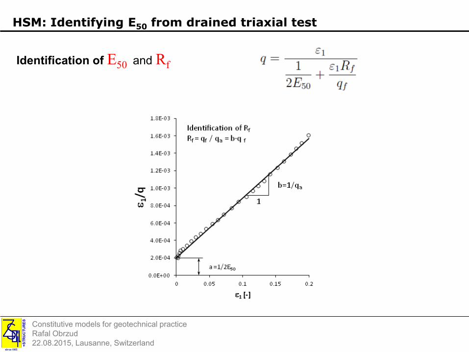
Identification of E50 and Rf
HSM: Identifying E50 from drained triaxial test
Constitutive models for geotechnical practice
Rafal Obrzud
22.08.2015, Lausanne, Switzerland
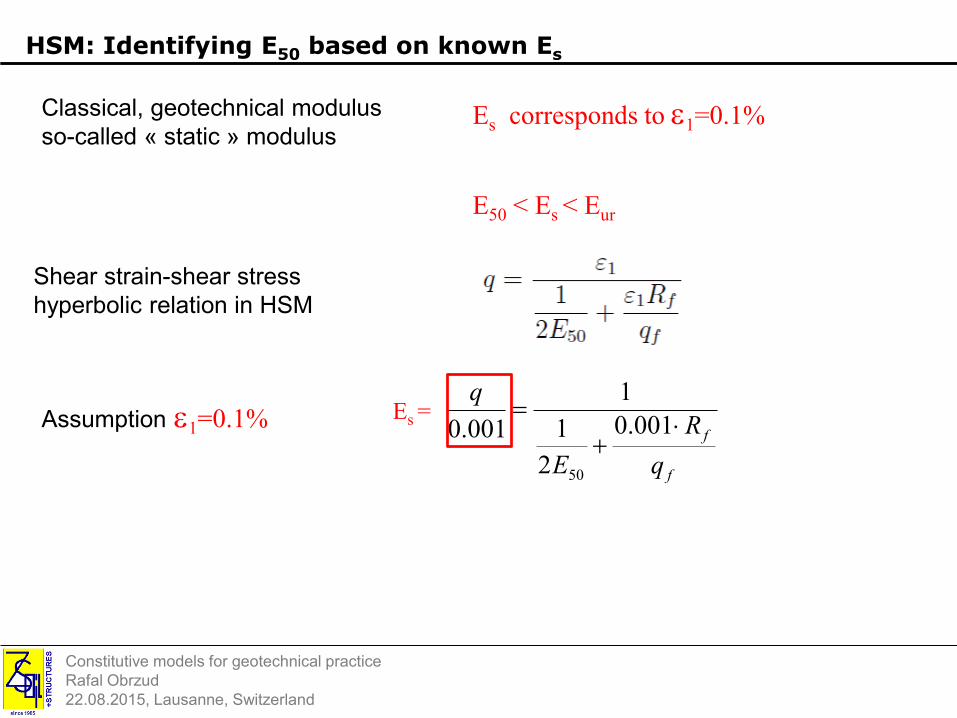
HSM: Identifying E50 based on known Es
Shear strain-shear stress
hyperbolic relation in HSM
E50 < Es < Eur
Classical, geotechnical modulus
so-called « static » modulusEs corresponds to e1=0.1%
f
f
q
R
E
q
001.0
2
1
1
001.0
50
Assumption e1=0.1% Es =

Constitutive models for geotechnical practice
Rafal Obrzud
22.08.2015, Lausanne, Switzerland
HSM: Identifying E50 based on known Es
1
1.1
1.2
1.3
1.4
1.5
1.6
1.7
1.8
1.9
2
10 20 30 40 50
E s/
E 50
fo
r s
3 =
10
0kP
a
Friction angle [deg]
),(
001.0
2
1
1
50 cq
R
E
E
f
fs
f

Constitutive models for geotechnical practice
Rafal Obrzud
22.08.2015, Lausanne, Switzerland
0
200
400
600
800
1000
1200
0.00% 5.00% 10.00% 15.00%
Dev
iato
ric
stre
ss [
kPa]
q
= s
1-s
3
Axial Strain e1
Triaxial drained compression test - Texas sand
SIG3 = 34.5kPa
SIG3 = 138kPa
SIG3 = 345kPa
E(1)
E(2)
E(3)
Hardening Soil: Stress dependent stiffness
s3(1) < s3
(2) < s3(3)
E(1) < E(2) < E(3)
59

Constitutive models for geotechnical practice
Rafal Obrzud
22.08.2015, Lausanne, Switzerland
E0ref , E50
ref, , Eurref correspond to reference minor stress sref
where
i.e. stiffness degrades with decreasing s3
up to the limit minor stress sL
NB.Setting m=0 -> constant stiffness like in the standard M-C model
Hardening Soil: Stress dependent stiffness
60

Constitutive models for geotechnical practice
Rafal Obrzud
22.08.2015, Lausanne, Switzerland
1. Find three values of E50(i) corresponding s3
(i) to respectively
2. Find a trend line y = ax + b by assigning variables
y =
x =
3. Then the determined slope of the trendline a is the parameter m
- HS Standard
HSM: Identyfikacja parametru m
q = s1-s3
s3
II identification method for E50

Constitutive models for geotechnical practice
Rafal Obrzud
22.08.2015, Lausanne, Switzerland
Hardening Soil: Stress dependent stiffness – Setting sref
sref -reference minor stress so if K0 < 1 then s’3 s’h
62
Let’s assume that the geotechnical report suggests assuming the stiffnessmodulus E for a given layer which is located at given depth …
1. Define what is given E with respect to E50 and Eur
2. Evaluate reference stress sref
Constitutive models for geotechnical practice
Rafal Obrzud
22.08.2015, Lausanne, Switzerland
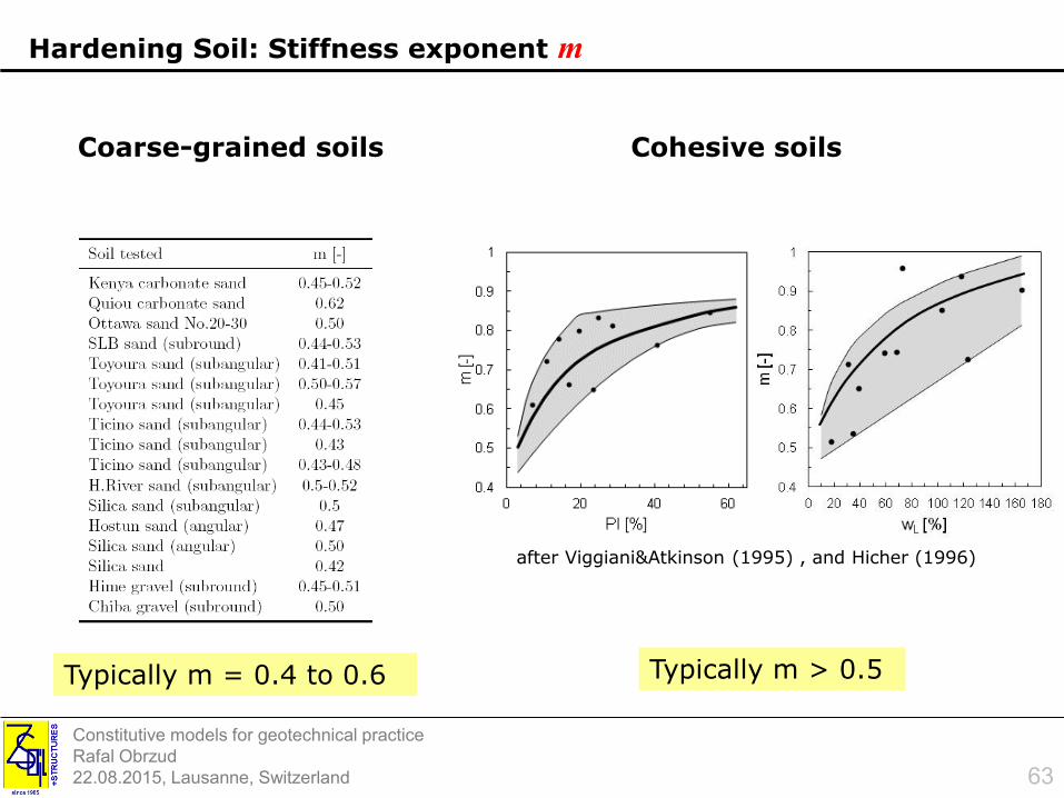
Hardening Soil: Stiffness exponent m
after Viggiani&Atkinson (1995) , and Hicher (1996)
Cohesive soilsCoarse-grained soils
Typically m > 0.5 Typically m = 0.4 to 0.6
63

Constitutive models for geotechnical practice
Rafal Obrzud
22.08.2015, Lausanne, Switzerland
0.0
2.0
4.0
6.0
8.0
10.0
12.0
14.0
16.0
18.0
20.0
0 50000 100000 150000 200000
z [m
]
E [kPa]
m = 0.4
m = 0.6
m = 0.8
0.0
2.0
4.0
6.0
8.0
10.0
12.0
14.0
16.0
18.0
20.0
0 50000 100000 150000 200000
z [m
]
E [kPa]
phi = 20
phi = 30
phi = 40
0.0
2.0
4.0
6.0
8.0
10.0
12.0
14.0
16.0
18.0
20.0
0 50000 100000 150000 200000
z [m
]
E [kPa]
c = 0
c = 15
c = 30
Level of reference stress
Hardening Soil: Stress dependent stiffness at initial state
During computation, stiffness moduli will evolve
according to actual stress magnitudes
64

Constitutive models for geotechnical practice
Rafal Obrzud
22.08.2015, Lausanne, Switzerland
A typical value for the elastic unloading/reloading Poisson’s ratio of nur = 0.2 can be
adopted for most soils.
Hardening Soil: Unloading/reloading Poisson’s ratio nur
65
Constitutive models for geotechnical practice
Rafal Obrzud
22.08.2015, Lausanne, Switzerland
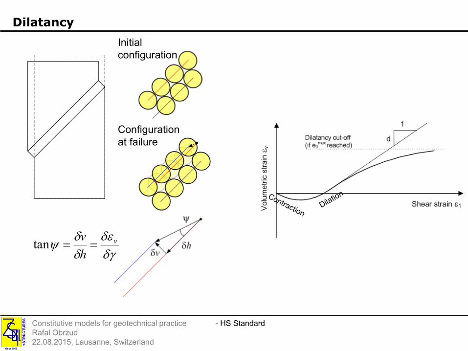
- HS Standard
Dilatancy
Initial
configuration
Configuration
at failure
d
de
d
d v
h
vtan

Constitutive models for geotechnical practice
Rafal Obrzud
22.08.2015, Lausanne, Switzerland
- HS Standard
Dilatancy

Constitutive models for geotechnical practice
Rafal Obrzud
22.08.2015, Lausanne, Switzerland
Dilatancy in HS model
Non-associated flow for
deviatoric mechanism
Mobilized dilatancy m increases
from 0 up to the input dilatancy
angle once M-C line is reached
Associated flow for volumetric
mechanism
Contractancy increases from zero
to maximum value at M-C failure
only when cap is mobilized

Constitutive models for geotechnical practice
Rafal Obrzud
22.08.2015, Lausanne, Switzerland
Typical dilatancy angles
Cohesive soils
Coarse soils

Constitutive models for geotechnical practice
Rafal Obrzud
22.08.2015, Lausanne, Switzerland
Experimental measurements from local strain gauges show that the initial values of
Poisson’s ratio in terms of small mobilized stress levels q/qmax varies between 0.1 and 0.2 for
clays, sands.
0.0
0.1
0.2
0.3
0.4
0.5
0 0.1 0.2 0.3 0.4 0.5 0.6 0.7 0.8 0.9 1
-e 3
/ e 1
[-]
Mobilized stress level q / qmax
Toyoura Sand (Dr=56%) Ticino Sand (Dr=77%)
Pisa Clay (Drained Triaxial) Sagamihara soft rock
Typically elastic domain
results after Mayne et al. (2009)
Hardening Soil: Unloading/reloading Poisson’s ratio nur
70

Constitutive models for geotechnical practice
Rafal Obrzud
22.08.2015, Lausanne, Switzerland
H controls the rate of volumetric
plastic strains
Evolution of the hardening
parameter pc :
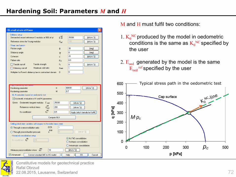
Hardening Soil: Parameters M and H
71
d𝜀𝑣𝑝
Constitutive models for geotechnical practice
Rafal Obrzud
22.08.2015, Lausanne, Switzerland
Typical stress path in the oedometric test
M and H must fulfil two conditions:
1. K0NC produced by the model in oedometric
conditions is the same as K0NC specified by
the user
2. Eoed generated by the model is the same
Eoedref specified by the user
Hardening Soil: Parameters M and H
72

Constitutive models for geotechnical practice
Rafal Obrzud
22.08.2015, Lausanne, Switzerland
Eoedref E50
ref
srefsoedref = sref / K0
NC
Hardening Soil: selection of oedometric modulus Eoed
In case of lack of oedometric test data for granular
material the oedometric modulus can approximately
be taken as:
Eoedref ≈E50
ref
if so soedref should be matched to the reference
minor stress sref since the latter typically
corresponds to the confining (horizontal) pressure
On the other hand, when defining
soedref sref in the model, the
following relationship should be
taken:
Eoedref ≈E50
ref (K0NC)m
73

Constitutive models for geotechnical practice
Rafal Obrzud
22.08.2015, Lausanne, Switzerland
where Cc is the compression index
Since we look for tangent Eoed, Ds’0, and
s*=2.303soedref
Hardening Soil: Tangent oedometric modulus Eoed
74

Constitutive models for geotechnical practice
Rafal Obrzud
22.08.2015, Lausanne, Switzerland
0
0.02
0.04
0.06
0.08
0.1
0.12
1 10 100 1000
Vo
lum
etri
c st
rain
e v
[-]
Vertical stress sv' [ kPa]
Simulation
Experiment
Vertical preconsolidationpressure s‘vc
Notion of overconsolidationratio:
Typical oedometer test
s‘v0 – current in situ stress
s‘vc – past vertical preconsolidation pressure
NB. In natural soils, overconsolidation
may stem from mechanical unloading
such as erosion, excavation, changes in
ground water level, or due to other
phenomena such as desiccation,
melting of ice cover, compression and
cementation.
Initial state variables - OCR
sv
75
𝐎𝐂𝐑 =𝝈𝒗𝒄′
𝝈𝒗𝟎′

Constitutive models for geotechnical practice
Rafal Obrzud
22.08.2015, Lausanne, Switzerland
Laboratory:
- Oedometer test (Casagrande’s method, Pacheco Silva
method (1970), cf. report on HS model)
Field tests:
- Static piezocone penetration (CPTU)
(for correlations see report on HS model in Zsoil Help)
- Marchetti flat dilatometer (DMT)
(correlations by Marchetti (1980), Lacasse and Lunne,
1988), see report on HS model in Zsoil Help)
Estimation of preconsolidation pressure and OCR
sv
76

Constitutive models for geotechnical practice
Rafal Obrzud
22.08.2015, Lausanne, Switzerland
K0NC consolidation – most cases of natural soils; the
value is automatically copied from
Isotropic consolidation – for running triaxial
compression test after isotropic consolidation
Anisotropic consolidation – for running triaxial
compression test after anisotropic consolidation
Initial state variables – OCR and K0
77

Constitutive models for geotechnical practice
Rafal Obrzud
22.08.2015, Lausanne, Switzerland
A – past stress s’SR
B – current in situ stress s’0
Horizontal
effective stress
Vertical
effective
stress
s’v
s’h
A B
s’v
s’h
A
B
p’
q
Excavation
Initial state variables – K0 and K0NC
K0NC
s’h0
s’v0
s’c
K0SR K0
NC
K0
nur
1-nur
qPOP
78

Constitutive models for geotechnical practice
Rafal Obrzud
22.08.2015, Lausanne, Switzerland
Preconsolidation stress configuration
corresponding to K0NC
Current in situ stress configuration
corresponding to K0(at the beginning of numerical simulation)
s’ SR
s’0
Initial state variables – K0 and K0NC
79

Constitutive models for geotechnical practice
Rafal Obrzud
22.08.2015, Lausanne, Switzerland
Estimation of earth pressure at rest
Normally-consolidated soils
0.2
0.3
0.4
0.5
0.6
0.7
0.8
0.9
0 20 40 60
K0
NC
f' [deg]
1-sin(phi')
Brooker&Ireland(1965)
Simpson(1992)
Overconsolidated soils
0.0
0.5
1.0
1.5
2.0
2.5
0 5 10 15 20
K0
OCR [-]
phi=20deg
phi=30deg
phi=40deg
Initial state variables – K0 vs. OCR
so-called (Jaky’s formula)
80

Constitutive models for geotechnical practice
Rafal Obrzud
22.08.2015, Lausanne, Switzerland
1. Through K0 (Materials)
2. Through Initial Stress (PrePro->FE->Initial conditions)
sy = “depth”
sx = sxK0(x)
Setting initial effective stresses
81

Constitutive models for geotechnical practice
Rafal Obrzud
22.08.2015, Lausanne, Switzerland
What to do if a model does not converge at
Initial State even though for a specified K0
1. try to start Initial State analysis from a small
Initial loading Fact. and Increment
2. otherwise, define initial conditions through
Initial Stresses option
Setting initial state variables - troubleshooting
Numerics, like engineers,
they like regularity and elegancy.
Privilege regular meshes
to avoid spourious oscillations
and lack of convergence.
82
embanking – troubleshooting
by means of Initial stresses

Constitutive models for geotechnical practice
Rafal Obrzud
22.08.2015, Lausanne, Switzerland
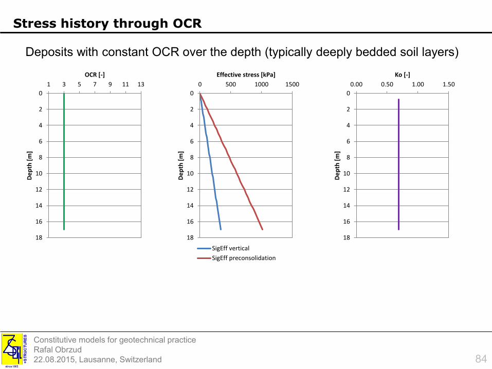
1. through OCR (gives constant OCR profile)
At the beginning of FE analysis, Zsoil sets the stress reversal point (SR) with:
2. through qPOP (gives variable OCR profile)
Initial state variables – preconsolidation effect
83
Constitutive models for geotechnical practice
Rafal Obrzud
22.08.2015, Lausanne, Switzerland
0
2
4
6
8
10
12
14
16
18
1 3 5 7 9 11 13
De
pth
[m
]
OCR [-]
0
2
4
6
8
10
12
14
16
18
0 500 1000 1500
De
pth
[m
]
Effective stress [kPa]
SigEff vertical
SigEff preconsolidation
0
2
4
6
8
10
12
14
16
18
0.00 0.50 1.00 1.50
De
pth
[m
]
Ko [-]
Deposits with constant OCR over the depth (typically deeply bedded soil layers)
Stress history through OCR
84

Constitutive models for geotechnical practice
Rafal Obrzud
22.08.2015, Lausanne, Switzerland
Profiles for Bothkennar clay
Deposits with varying OCR over the depth (typically superficial soil layers)
85

Constitutive models for geotechnical practice
Rafal Obrzud
22.08.2015, Lausanne, Switzerland
0
2
4
6
8
10
12
14
16
18
0 0.5 1 1.5
De
pth
[m
]
Ko [-]
0
2
4
6
8
10
12
14
16
18
1 3 5 7 9 11 13
De
pth
[m
]
OCR [-]
0
2
4
6
8
10
12
14
16
18
0 200 400 600
De
pth
[m
]
Effective stress [kPa]
SigEff vertical
SigEff preconsolidation
qPOP
K0OC = K0
NC OCR
K0OC = K0
NC OCRsin(f) (Mayne&Kulhawy 1982)
Variable K0 can be introduced merely through Initial Stress option
Deposits with varying OCR over the depth (typically superficial soil layers)
Stress history through qPOP
86

Constitutive models for geotechnical practice
Rafal Obrzud
22.08.2015, Lausanne, Switzerland
Versatility of Hardening Soil model
87
Good approximation of stress-strain relation for different and complex stress
paths that can be encountered in geotechnical engineering

Constitutive models for geotechnical practice
Rafal Obrzud
22.08.2015, Lausanne, Switzerland
Hardening Soil Model - Report
88

Constitutive models for geotechnical practice
Rafal Obrzud
22.08.2015, Lausanne, Switzerland
Report contents
Short introduction to the HS models (theory)
Parameter determination
Experimental testing requirements for direct parameter identification
Alternative parameter estimation for granular materials
Alternative parameter estimation for cohesive materials
Benchmarks
Case studies including parameter determination
retaining wall excavation
tunnel excavation
shallow footing
The HS model – a practical guidebook
89

Constitutive models for geotechnical practice
Rafal Obrzud
22.08.2015, Lausanne, Switzerland
Introduction
Initial stress state and definition of effective stresses
Saturated and partially-saturated two-phase continuum
Introduction to the Hardening Soil model (HSM)
Undrained behavior analysis using HSM
Practical applications of HSM
Contents
90

Constitutive models for geotechnical practice
Rafal Obrzud
22.08.2015, Lausanne, Switzerland
Hardening Soil model is formulated in effective stresses (s’1, s’2, s’3 and p’)
and therefore it requires:
o Effective stiffness parameters E′0, E′ur, E′50, n′ur
o Effective strength parameters f’, c’
Undrained or Partially drained conditions can be obtained by in Deformation+Flow, Consolidation type analysis depending on action
time and adequate permeability coefficients
Undrained behavior analysis (1st approach)
91
Advantages:1. Partial saturation effects included2. Possibility of running any analysis type after consolidation analysis

Constitutive models for geotechnical practice
Rafal Obrzud
22.08.2015, Lausanne, Switzerland
Undrained behavior analysis
92
Schematic representation of shear strength for normally-consolidated material in drained and undrained conditions

Constitutive models for geotechnical practice
Rafal Obrzud
22.08.2015, Lausanne, Switzerland
Undrained behavior can be simulated in effective stress analysis Deformation+Flow, Driven Load (Undrained)
Undrained behavior analysis (2nd approach)
93
It follows any other like Driven load+Steady state, Driven load+Transientor Consolidation then the condition for the suction pressure is verified for pressure
p = S(p0) p0 + Dp
(Dp is produced exclusively by the undrained driver.). In order to trace the evolution of the
pore pressure values stored at the element integration point must be used so:
Disadvantages1. Undrained driver cannot be followed by any other driver
Advantages:1. Fully undrained behavior (no volume change) with effective stress parameters2. Useful for dynamics

Constitutive models for geotechnical practice
Rafal Obrzud
22.08.2015, Lausanne, Switzerland
Setting undrained behaviour for Driven Load(Undrained)
94
Clay
Sand
Mixed drainage conditions

Constitutive models for geotechnical practice
Rafal Obrzud
22.08.2015, Lausanne, Switzerland
Undrained behavior in total stress analysis can also be performed for the HS model using total stress strength parameters, i.e.
f 0°, c = Su, 0°)
E′0, E′ur, E50ud, n=0.499 (undrained conditions)
Set high OCR, e.g. 1000 to disable cap mechanism (no plastic volumetric
deformations)
however
o sequence of parameter setup should be followed (given below)
o appropriate analysis type should be selected (Deformation)
o Limitations …
Undrained behavior analysis (3rd approach - simplified)
95

Constitutive models for geotechnical practice
Rafal Obrzud
22.08.2015, Lausanne, Switzerland
Undrained behavior analysis – single phase analysis using HS
Parameter setup for undrained simulation with single phase analysis:
1. Insert effective parameters E′0, E′ur in Elastic menu.
2. Disable Automatic evaluation of H and M parameters
(to avoid autoeval. while closing the dialog and errors
due to null friction angle)
3. Set high OCR, e.g.1000, to disable cap mechanism (no plastic volumetric deformations
should be produced due to assumed undrained conditions)
4. Change f′ and c′ into ”undrained” parameters f = 0° and c = Su. In order to ensure stability of
numerical computing, specify = 0°
5. Considering that the undrained conditions imply s1 = s3, change n′ur into nur = 0.4999 (the
”undrained” stiffness behavior will be obtained in the analysis by recomputing the stiffness
tensor with nur = 0.4999
96

Constitutive models for geotechnical practice
Rafal Obrzud
22.08.2015, Lausanne, Switzerland
Undrained behavior analysis – single phase analysis using HS
97
Parameter setup for undrained simulation
with single phase analysis:
6. Set input E50 as undrained E50ud (but not Eur and E0 which should remain as effective ones)
shear modulus is not affected by the drainage condition so one can write:
where nu is the Poisson's coffecient in undrained conditions equalk to 0.499.
So the above equation can be rewritten for E50 as:
)1(2
'3 5050
EEu
where n should be considered as that corresponding to E’50 , i.e. n 0.3 (plastic deformations)
Constitutive models for geotechnical practice
Rafal Obrzud
22.08.2015, Lausanne, Switzerland
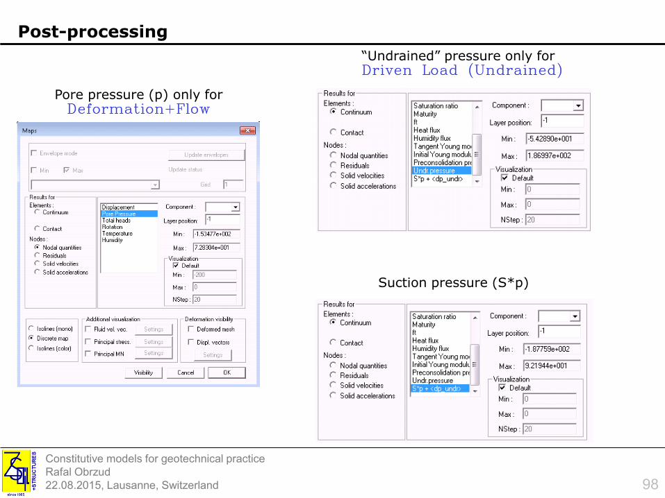
Post-processing
98
“Undrained” pressure only forDriven Load (Undrained)
Suction pressure (S*p)
Pore pressure (p) only forDeformation+Flow

Constitutive models for geotechnical practice
Rafal Obrzud
22.08.2015, Lausanne, Switzerland
Introduction
Initial stress state and definition of effective stresses
Saturated and partially-saturated two-phase continuum
Introduction to the Hardening Soil model (HSM)
Undrained behavior analysis using HSM
Practical applications of HSM
Assistance in parameter identification
Contents
99

Constitutive models for geotechnical practice
Rafal Obrzud
22.08.2015, Lausanne, Switzerland
Practical applications – Shallow footing on an overconsolidated sand
(Help/Reports/Hardening Soil small -> Benchmarks/Spread footing on overconsolidated sand)
Input files:HS-small-Footing-Texas-Sand-2phase.inp
Input files:HS-small-Footing-Texas-Sand-2phase.inp
100

Constitutive models for geotechnical practice
Rafal Obrzud
22.08.2015, Lausanne, Switzerland
5. Interpreting and Setting K0
Variable K0 can be introduced merely through Initial Stress option
Practical applications – Shallow footing on an overconsolidated sand
101

Constitutive models for geotechnical practice
Rafal Obrzud
22.08.2015, Lausanne, Switzerland
4. Selecting qPOP 5. OCR based on qPOP
Variable OCR profile
Practical applications – Shallow footing on an overconsolidated sand
102

Constitutive models for geotechnical practice
Rafal Obrzud
22.08.2015, Lausanne, Switzerland
Practical applications – Shallow footing on an overconsolidated sand
Comparison of models: HS-SmallStrain, HS-Std vs Mohr-Coulomb
103

Constitutive models for geotechnical practice
Rafal Obrzud
22.08.2015, Lausanne, Switzerland
Engineering draft and the sequence of excavation
Practical applications – Excavation in Berlin sand
Input files:HS-small-Exc-Berlin-Sand-2phase.inp
HS-std-Exc-Berlin-Sand-2phase.inp
MC-Exc-Berlin-Sand-2phase.inp
Input files:HS-small-Exc-Berlin-Sand-2phase.inp
HS-std-Exc-Berlin-Sand-2phase.inp
MC-Exc-Berlin-Sand-2phase.inp
104

Constitutive models for geotechnical practice
Rafal Obrzud
22.08.2015, Lausanne, Switzerland
Standard Mohr-Coulomb Hardening-Soil
Berlin sand excavation
Practical applications – Excavation in Berlin sand
Absolute displacements
105

Constitutive models for geotechnical practice
Rafal Obrzud
22.08.2015, Lausanne, Switzerland
Standard Mohr-Coulomb
HS SmallStrain
Practical applications – Excavation in Berlin sand
settlements
lifting
« Stiff »
zone
of Gmax
True zone of influence
Accumulation of
spurious strains
HS without E0
extended zone of influence
Vertical displacements
at soil surface
NB. HS SmallStrain makes
it possible to reduce the
extension of the FE mesh
106

Constitutive models for geotechnical practice
Rafal Obrzud
22.08.2015, Lausanne, Switzerland
Practical applications – Excavation in Berlin sand
Meaning of stress level in HS model
Displayed stress levels are computed as:
SL = q / qf
q – current deviatoric stress at given p’
qf – failure stress corresponding to p’
107

Constitutive models for geotechnical practice
Rafal Obrzud
22.08.2015, Lausanne, Switzerland
Introduction
Initial stress state and definition of effective stresses
Saturated and partially-saturated two-phase continuum
Introduction to the Hardening Soil model (HSM)
Undrained behavior analysis using HSM
Practical applications of HS
Assistance in parameter identification
Contents
108

Constitutive models for geotechnical practice
Rafal Obrzud
22.08.2015, Lausanne, Switzerland
Virtual Lab
109
a highly-interactive tool for assistance in parameter
selection for constitutive models for soils
first-guess for model parameters for any incomplete or
complete material data
automatic or interactive knowledge extraction
parameter identification from laboratory curves
provides parameter ranges (parametric studies)
testing constitutive models

Constitutive models for geotechnical practice
Rafal Obrzud
22.08.2015, Lausanne, Switzerland
Virtual Lab
110
Help → Reports Access
Toolbox available for:
• Hardening-Soil
• Mohr-Coulomb
• Cap
• Cam-Clay

Constitutive models for geotechnical practice
Rafal Obrzud
22.08.2015, Lausanne, Switzerland
Exercise 2 – Parameter identification from laboratory curves
111
1
1. Select the determinationmethod: Identification

Constitutive models for geotechnical practice
Rafal Obrzud
22.08.2015, Lausanne, Switzerland
Exercise 2 – Import experimental test data
112
1
3
3
3
In order to define a new laboratory test:
1. Preselect the type of test and press
Add
2. Give a label to the test and define
initial state variables
3. Import test results from an ASCII file
by pressing Import experimental data,
selecting the file, and assigningvariables to corresponding columns
2

Constitutive models for geotechnical practice
Rafal Obrzud
22.08.2015, Lausanne, Switzerland
Exercise 2 – Import experimental test data
113
Import prepared data files:
SandMedium-txcd-sig25kPa.pit
SandMedium-txcd-sig50kPa.pit
SandMedium-txcd-sig75kPa.pit
1A
1B
1A. In order to import prepared in advanceand saved experimental data for threetriaxial tests, click right button and select Load test(s)
1B. Select files and open them
2. Browse imported resuts by seleacting eachtest separately in Assembly of tests
Load test(s)
Constitutive models for geotechnical practice
Rafal Obrzud
22.08.2015, Lausanne, Switzerland
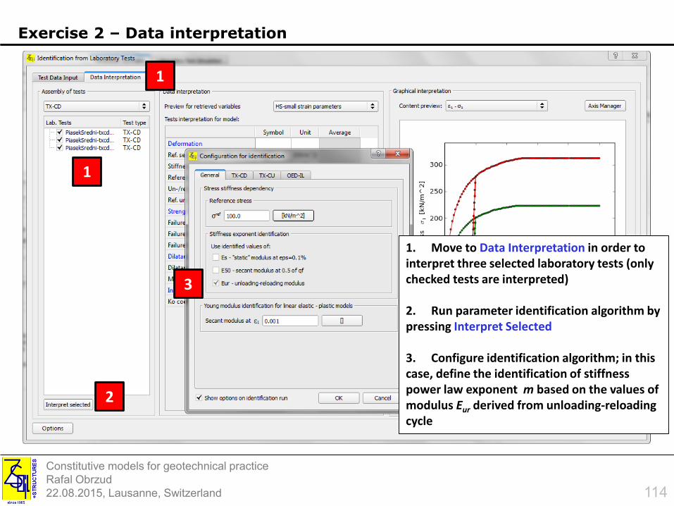
Exercise 2 – Data interpretation
114
1
2
3
1. Move to Data Interpretation in order to interpret three selected laboratory tests (onlychecked tests are interpreted)
2. Run parameter identification algorithm by pressing Interpret Selected
3. Configure identification algorithm; in thiscase, define the identification of stiffnesspower law exponent m based on the values of modulus Eur derived from unloading-reloadingcycle
1
Constitutive models for geotechnical practice
Rafal Obrzud
22.08.2015, Lausanne, Switzerland
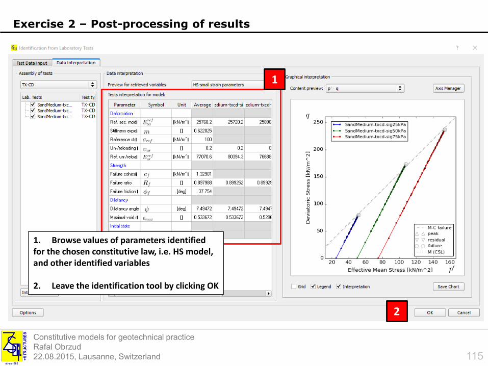
Exercise 2 – Post-processing of results
115
1. Browse values of parameters identifiedfor the chosen constitutive law, i.e. HS model, and other identified variables
2. Leave the identification tool by clicking OK
1
2

Constitutive models for geotechnical practice
Rafal Obrzud
22.08.2015, Lausanne, Switzerland
Exercise 2 – Post-processing of results
116
Constitutive models for geotechnical practice
Rafal Obrzud
22.08.2015, Lausanne, Switzerland
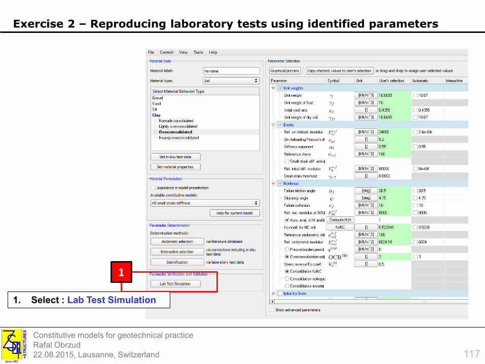
Exercise 2 – Reproducing laboratory tests using identified parameters
117
1
1. Select : Lab Test Simulation

Constitutive models for geotechnical practice
Rafal Obrzud
22.08.2015, Lausanne, Switzerland
Exercise 2 - Reproducing laboratory tests with identified parameters
118
1
2
4
5
1. Select drained test in the test preselection (TX-CD) and enable Use real test data to simulate the tests used for parameter identification (notice that the initial state variables and loadingprogram have been already defined).
2. Select one of tests3. Import parameters identified with TX-CD4. Press Simulate selected test5. Compare model responses with
laboratory curves
3