constrained optimization with low-rank tensors and … · constrained optimization with low-rank...
TRANSCRIPT
CONSTRAINED OPTIMIZATION WITH LOW-RANK TENSORSAND APPLICATIONS TO PARAMETRIC PROBLEMS WITH PDEs
SEBASTIAN GARREIS∗ AND MICHAEL ULBRICH†
Abstract. Low-rank tensor methods provide efficient representations and computations forhigh-dimensional problems and are able to break the curse of dimensionality when dealing withsystems involving multiple parameters. Motivated by optimal control problems with PDEs underuncertainty, we present algorithms for constrained nonlinear optimization problems that use low-ranktensors. They are applied to optimal control of PDEs with uncertain parameters and to parametrizedvariational inequalities of obstacle type. These methods are tailored to the usage of low-rank ten-sor arithmetics and allow to solve huge scale optimization problems. In particular, we consider asemismooth Newton method for an optimal control problem with pointwise control constraints andan interior point algorithm for an obstacle problem, both with uncertainties in the coefficients.
Key words. Nonlinear optimization, low-rank tensors, PDEs with uncertainties, optimal con-trol under uncertainty, parametric variational inequalities, uncertainty quantification, semismoothNewton methods, interior point methods
1. Introduction. In this paper we develop low-rank tensor methods for solvingproblems that arise from discretizations of inequality-constrained optimization prob-lems that involve PDEs with uncertain parameters. Especially, we consider optimalcontrol of a PDE under uncertainty for obtaining robust optimal solutions. Further,we address the computation of the whole parametric solution of variational inequalities(VIs) of obstacle type involving uncertainties. This provides a basis for uncertaintyquantification (UQ) of solutions to these VIs. In combination, our results for bothproblem classes prepare the ground towards using low-rank tensor methods for, e.g.,dealing with state constraints under uncertainty, optimizing the conditional value-at-risk (CVaR) or related risk measures, or tackling optimal control problems governedby VIs under uncertainty.
Low-rank tensors. In many application areas tensors can be used to describethe multivariate state of a system, for example when dealing with many parameterslike in uncertainty quantification or with many free variables like in quantum mechan-ics. In the finite-dimensional case a tensor is a multidimensional array, which, e.g.,can represent a multivariate function by its values on a structured grid. If there ared dimensions and n degrees of freedom per dimension, then the resulting tensor hasnd components. Storage and computational time thus scale like O(nd). The curse ofdimensionality caused by the exponential dependence on the order d renders workingwith full tensors intractable already for moderate orders. Thus, more efficient tensorrepresentations are required, and for instance in quantum physics such approachesare in use for quite some time already, see, e.g., [30, 41]. In the last years, significantprogress has been made in the development of a mathematically rigorous theory andalgorithms for such low-rank tensor formats, see, e.g., [21, 22, 33] for an overview.Classical tensor decompositions either lack important theoretical properties or havecomplexity issues. Current investigations therefore deal with the approximation oftensors in new low-rank formats that combine low complexity with good theoreticaland computational properties. In particular, the tensor train (TT) format [46, 47] and
∗Technical University of Munich, Chair of Mathematical Optimization, Department of Mathe-matics, Boltzmannstr. 3, 85748 Garching b. Munchen, Germany ([email protected]).†Technical University of Munich, Chair of Mathematical Optimization, Department of Mathe-
matics, Boltzmannstr. 3, 85748 Garching b. Munchen, Germany ([email protected]).
1
2 S. Garreis and M. Ulbrich
the hierarchical Tucker (HT) decomposition [24, 39] meet the requirements of scalingwell in the order and the dimensions of the tensor. They also are attractive from atheoretical and algorithmic perspective. Currently, TT and HT approximations oftensors are intensively investigated, using different techniques such as generalizationsof the SVD [9, 20], pointwise evaluations [44, 5], and minimization of least squaresfunctionals. The latter requires optimization algorithms for unconstrained problemswith tensors of fixed or adaptive low rank, for example block coordinate descent meth-ods like (M)ALS [29], DMRG [45], and AMEn [12], or Riemannian optimization thatworks on low-rank tensor manifolds [8, 36]. Further recent work addresses the so-lution of large linear systems by iterative methods such as preconditioned conjugategradient (PCG) algorithms for tensors in the HT format [38]. All these algorithmsbenefit from the good complexity of low-rank tensors.
In contrast to the mentioned methods for unconstrained optimization, we proposealgorithms for inequality constrained optimization in this paper and apply them to op-timal control problems with PDEs under uncertainty and to variational inequalities ofobstacle type with uncertain coefficients. Exploiting the attractive complexity prop-erties of low-rank tensors, these algorithms are able to solve systems with multipleparameters. Compared to other methods that were recently applied in similar con-texts, low-rank tensors feature linear scaling in the number of parameters d. Sparsegrids, for instance, can also reduce the computational complexity drastically, but ingeneral still scale exponentially [19]. Further improvements are possible by construct-ing adaptive algorithms as in [34]. Monte Carlo (MC) type methods are known fortheir quite slow, but dimension-independent approximation properties. Accelerationtechniques for MC include Quasi-Monte Carlo [42, 40] or multi-level approaches [6].
Optimal control under uncertainty. A main motivation of this work areinequality-constrained optimal control problems governed by elliptic PDEs with un-certain coefficients: Let α ∈ Γ :=×m
i=1Γi ⊂ Rm be a random vector with indepen-
dently distributed components αi ∈ Γi ⊂ R and associated probability measures Pαion Γi. The random vector α is then distributed according to the probability measurePα :=
⊗mi=1 Pαi on Γ; we write α :=
∫Γα dPα for its expected value. The determin-
istic control u and, for any fixed α, the state yα live in the Banach spaces U and Y ,respectively. The state equation is given by
Eα(yα, u) := A(α)yα − b(u) = 0, (1)
with a control operator b : U → Y ∗, a parameter-dependent linear elliptic operatorA(α) : Y → Y ∗, and Eα : Y × U → Y ∗. We assume that (1) has a unique solutionyα(u) = A(α)−1b(u) for Pα-almost every (a.e.) α ∈ Γ and all u ∈ U and consider theoptimal control problem
min(yα)α∈Γ,u
σ(J1(yα, u)) + J2(u) s. t. Eα(yα, u) = 0, yα ∈ Yad (Pα-a.e. α ∈ Γ),
u ∈ Uad,(2)
with J1 : Y × U → R, J2 : U → R, and suitable nonempty closed convex admissiblesets Uad ⊂ U and Yad ⊂ Y for the control and the state, respectively. Note thatJ1(yα, u) depends on the random vector α and thus is a real-valued random variable.The application of a suitable risk measure σ (e.g., the expectation Eα [34] or the CVaR[35]) then yields a scalar-valued objective function. The parametric state equationand the state constraints shall hold for almost all (a.a.) α ∈ Γ.
Constrained Optimization with Low-Rank Tensors 3
Since the described problem class, involving general state and control constraintsand general risk measures, is too comprehensive to be addressed in a single paper, wesplit the considerations into two subclasses:
(a) optimal control problems with PDEs under uncertainty of the form (2) withcontrol constraints and a risk-neutral objective function, i.e., Yad = Y , σ = Eα.
(b) variational inequalities of obstacle type under uncertainty: For a.a. α,
yα ∈ Yad, 〈A(α)yα − b, v − yα〉Y ∗,Y ≥ 0 ∀ v ∈ Yad. (3)
with given b ∈ Y ∗ and the same parametric elliptic operator as in (1).By investigating (a) we show that optimal control problems of this type can be
efficiently solved by the proposed low-rank tensor techniques. The problem class (b),on the other hand, provides a prototypical setting for problems that involve Pα-a.s.pointwise inequality constraints on a parametric state yα.
For solving the problem classes numerically, there are several possibilities for thediscretization of the parameter-dependent state: In particular, Monte Carlo (MC)type sampling based techniques can be used. Alternatively, the tensor product struc-ture of Γ enables the use of sparse grids as done in [34]. In contrast to that,we view the parameter-dependent state as an element y of a tensor Banach spaceY = Y ⊗L2(Γ1,Pα1
)⊗ . . .⊗L2(Γm,Pαm) and discretize it by a full tensor product ofsubspaces (finite elements for U and Y and polynomials for α). This yields coefficientsy ∈ RN0×...×Nm in tensor form. To avoid the curse of dimensionality, we approximatethese tensors by either TT or HT low-rank tensor formats. They feature a linear com-plexity in m, but only offer a limited set of operations that can be computed efficientlywithin the format. Therefore, we have to design suitable optimization methods care-fully, especially if component-wise inequality constraints on y are involved, in orderto only use operations that are implementable with low-rank tensors.
For the problem class (a) (covered in section 3.1) we propose a semismooth New-ton method (section 4.1). The corresponding state and adjoint equation — bothare linear operator equations in tensor space — are solved without leaving the low-rank tensor format using AMEn [12], a block iterative method that operates on thecore tensors of the TT representation. For this purpose the discretized parametricPDE operator A(α) has to be applied to low-rank tensors efficiently, which is demon-strated in two examples (section 3). The reduced objective function and its gradientare evaluated based on the computed tensor state and adjoint state. A semismoothNewton method is applied to the optimality conditions of the reduced problem. Thesemismooth Newton system is solved by a block elimination and CG.
In the case that Yad encodes Pα-a.e. posed pointwise state constraints for thewhole tensor y, one has to deal with component-wise bound constraints for the tensory after discretization. The same holds true for the case Yad = Y and the nonsmoothrisk measure σ = CVaRβ since then the problem (2) can be reformulated as a smoothproblem where also pointwise bounds on a tensor arise, see [35, sec. 4]. To investigateif and how it is possible to successfully tackle these challenges we consider the problemclass (b). Specifically, we address the computation of the full parametric solution ofthe obstacle type VI (3) by a primal interior-point method (sections 3.2 and 4.2).Note that for the case that the operators A(α) are self-adjoint, (3) can equivalentlybe written as the following parametric optimization problem:
minyα∈Y
Fα(yα) := 12 〈A(α)yα, yα〉Y ∗,Y − 〈b, yα〉Y ∗,Y s. t. yα ∈ Yad. (4)
The first and second derivative of the log-barrier term require computing component-
4 S. Garreis and M. Ulbrich
wise reciprocals of tensors. For this we use a Newton-Schulz iteration or, alternatively,AMEn. The solution of the barrier-Newton system is done by either AMEn or by alow-rank tensor PCG method [38]. Feasible step lengths are determined by the com-putation of the maximum component of a tensor, for which we use global optimizationon the represented continuous function.
Overview of the paper. This paper is organized as follows: We give a briefintroduction to tensors and low-rank formats in the next section. Then, the twoproblem classes and example applications including their discretization are discussedin more detail (section 3). We present our algorithms for the solution of the problemsin section 4. The numerical tests in section 5 show their efficiency and accuracy.Conclusions and an outlook are given in section 6.
In the paper we use the following notation: Deterministic functions, e.g., thecontrol u, and corresponding operators and spaces are written in italic font, whereasfunctions that also depend on α, such as the state y, are bold and italic. We useroman fonts for functions from a finite-dimensional (discretized) space, e.g., u and y,and sans-serif fonts for the corresponding coefficient vectors (u) and tensors (y).
2. Tensors and low-rank formats. Since tensors will be used for the dis-cretization and solution of the described problems, we first introduce discrete tensorsand low-rank formats. For more extensive introductions, especially on low-rank for-mats, we refer, e.g., to the articles [21] or [4].
2.1. Basics and notation. In this paper, we denote by a tensor x ∈ Rn1×...×nd
a d-dimensional array of real numbers (cf. [39, sec. 1]). The array dimension d is calledthe order of the tensor and the modes are numbered by 1, . . . , d. We denote the di-mension of the i-th mode by ni and write x(k1, . . . , kd) for the (k1, . . . , kd)-componentof x, where ki ∈ [ni], i ∈ [d], writing [m] := {1, . . . ,m} here and throughout. Thetensors of all ones will be denoted by 1 if the dimensions are clear. Reshaping a tensoras a vector in a certain order will be written as vec(x) ∈ Rn1···nd . Matricization, i.e.,
reshaping as a matrix, is denoted by x(t) ∈ R(∏i∈t ni)×(
∏j /∈t nj), where t ⊂ [d] denotes
the set of modes that become the rows of the resulting matrix. Analogously we writeten(x) for reshaping a vector or a matrix x back into a tensor when the dimensionsare clear. For the extraction of parts of a tensor we also allow indexing with sets andwrite “·” for the full index range of a mode: x(·, 4, {1, 5},·, . . . ,·) ∈ Rn1×2×n4×...×nd
is obtained from x by fixing the second index at 4 and taking the first and fifth com-ponents of the third mode and all components of the remaining modes. Note thatmodes indexed by a single number are cut out in the result, while modes indexed bya set remain. As tensors form a vector space, all vector space operations are definedfor them. Additionally, component-wise operations are useful: x � y denotes multi-plication, x � y division and x.λ exponentiation. The component-wise application ofa function f : R→ R is written as f(x).
Definition 2.1 (i-mode matrix product). Let x ∈ Rn1×...×nd be a tensor, i ∈ [d]a mode, and A : Rni → Rm a linear operator (or a matrix). Then the i-mode ma-trix product A ◦i x ∈ Rn1×...×ni−1×m×ni+1×...×nd is defined by (A ◦i x) (k1, . . . , kd) :=(Ax(k1, . . . , ki−1,·, ki+1, . . . , kd)) (ki) for all (k1, . . . , kd) ∈ [n1] × . . . × [ni−1] × [m] ×[ni+1]× . . .× [nd]. In short notation: A ◦i x = ten
(Ax({i})) (cf. [39, sec. 4.1]).
This definition means that we take all vectors that result from fixing all indices ofthe tensor x except the i-th one, apply A, and use the resulting vectors to form A ◦i x.We view tensors of order 1 as column vectors and order-2-tensors as matrices wherethe first index is for the rows. The contraction of two tensors is a further important
Constrained Optimization with Low-Rank Tensors 5
operation. It generalizes inner and outer products as well as matrix multiplication.Definition 2.2 (tensor contraction). Let x ∈ Rn1×...×nd and z ∈ Rn1×...×nd be
tensors and s = (s1, . . . , sp), t = (t1, . . . , tp) with si ∈ [d], ti ∈ [d], nsi = nti be ordered
lists of modes. Further, let si, 1 ≤ i ≤ d− p, and ti, 1 ≤ i ≤ d− p, be the remainingmodes in ascending order. Then the contraction 〈x, z〉s,t ∈ Rs1×...×sd−p×t1×...×td−p ofx and z along the modes s and t is defined as
〈x, z〉s,t(ks1 , . . . , ksd−p , `t1 , . . . , `td−p) =
ns1 ,...,nsp∑ks1 ,...,ksp=1
x(k1, . . . , kd)z(`1, . . . , `d)|`ti=ksi∀i∈[p]
component-wise for all indices ksi ∈ [nsi ] (i ∈ [d − p]) and `tj ∈ [ntj ] (j ∈ [d − p]).When t or s are sets, they stand for the lists of components in ascending order.
Here, similar to a matrix product, a component of the contraction is obtained byfixing indices in the untouched modes and computing the inner product of the equallysized subtensors. The following special cases of tensor contraction are useful:
Definition 2.3 (special cases of tensor contraction). Let x, y ∈ Rn1×...×nd andz ∈ Rn1×...×nd be tensors.
• The outer product1 x ⊗ z := 〈x, z〉∅,∅ ∈ Rn1×...×nd×n1×...×nd of the tensors xand z is obtained as (x⊗ z) (k1, . . . , kd, `1, . . . , `d) = x(k1, . . . , kd)z(`1, . . . , `d).
• An elementary tensor (or rank-1-tensor)⊗d
i=1 ui ∈ Rn1×...×nd is an outer
product of vectors:(⊗d
i=1 ui)
(k1, . . . , kd) =∏di=1 u
iki, where uiki is the ki-th
component of the vector ui ∈ Rni .• The inner product 〈x, y〉 := 〈x, y〉[d],[d] ∈ R of two tensors of the same size is〈x, y〉 =
∑n1
k1=1 . . .∑ndkd=1 x(k1, . . . , kd)y(k1, . . . , kd).
• The Frobenius norm of a tensor x is ‖x‖F :=√〈x, x〉.
The i-mode matrix product is a matrix-tensor contraction: A ◦i x = 〈A, x〉{2},{i}.
2.2. Low-rank tensor formats. As the amount of data of a full tensor is ingeneral very high (of order
∏di=1 ni = O(ndmax) with nmax := maxi∈[d] ni, i.e., expo-
nential in d), current investigations deal with representations or approximations ofit that require substantially less memory. In the classical canonical polyadic (CP)decomposition [28, 49], the tensor is approximated by a sum of R elementary ten-sors, where R is the tensor rank. The required storage O(Rnmaxd) is linear in d.But this format has some drawbacks such as the possible ill-posedness of the bestapproximation by CP tensors of rank ≤ R [10].
In the matrix case d = 2 an optimal low-rank approximation can be computedby a truncated singular value decomposition (SVD). The approximation error can beexpressed in terms of the singular values [13]. There exist several generalizations ofthis approximation technique to d-dimensional tensors. All of them are formats withtree structure (see [4]) where the approximation problem is well-posed in contrast tothe CP format. In the classical Tucker format [52], the higher order SVD (HOSVD)truncates a tensor to lower Tucker rank giving a quasi-optimal result2 and offers errorcontrol similar to standard SVD [9]. Here, and also for other tensor formats, the
1Note that the vectorization/matricization of the outer product of two tensors coincides with thestandard Kronecker product (also denoted by ”⊗”) of vectorizations/matricizations of them.
2Best approximation up to a factor that depends on the order d of the tensor (√d for the Tucker
format, see, e.g., [21]).
6 S. Garreis and M. Ulbrich
required tensor rank depends on the truncation tolerance. The Tucker format still isexponential in d since it uses a core tensor c ∈ Rr1×...×rd .
The latter issue can be solved by representing the tensor x by a contraction oftensors of order ≤ 3 as done, e.g., in the tensor train (TT) format [46]. The TTrank of a tensor x ∈ Rn1×...×nd is a vector r := (r0, r1, . . . , rd) with r0 = rd = 1 andri ∈ N for i ∈ {2, . . . , d−1}. In the TT format, x = TT (u) is represented by a d-tuple
u := (u1, . . . ,ud) ∈×d
i=1Rri−1×ni×ri of order-3-tensors as follows:
x(k1, . . . , kd) = u1(·, k1,·)u2(·, k2,·) · · ·un(·, kn,·) ∈ R ∀ ki ∈ [ni], i ∈ [d].
Note that this is a simple product of matrices, resulting in a scalar value becausethe first and the last matrix of the chain are a row and column vector, respectively.The tensor x is therefore a contraction of the tensors ui. The storage requirement isO(dnmaxr
2max), hence linear in d, where nmax and rmax are upper bounds for the ni
and ri. The TT-Toolbox [47] provides implementations in Matlab and in Python.In the related hierarchical Tucker (HT) decomposition [24], such a contraction
of smaller tensors is performed according to a more general, binary dimension tree.This results in a similarly nice structure and complexity as the TT format as well asin comparable available arithmetic operations. The htucker toolbox [39] implementstensors in this format and – similarly to the TT-Toolbox – efficient versions of themost important operations, e.g., extraction of parts of the tensor, application of linearoperators to the i-th mode, contraction, tensor orthogonalization and truncation to alower rank by the SVD-based hierarchical SVD (HSVD) [20] with error control andquasi-optimal approximation up to the factor
√2d− 3. This truncation (rounding) is
crucial because when using the standard implementations for summing or multiplyingtwo HT tensors component-wise, the ranks sum or multiply, respectively. Therefore,special truncated versions of these operations are available. All these operationscan be performed with a reasonable time complexity (linearly in nmax and d andpolynomially in rmax). The same holds for tensors in TT format.
As our algorithms use operations and subsolvers that currently are not all availablewithin a single format or toolbox, our implementations use HT tensors with a linear,TT-like dimension tree (as provided by htucker). This allows to convert between theHT and TT formats (cf. [22, sec. 12.2.2]).
3. Applications: problem formulation and discretization. We will use thegood complexity of low-rank tensors to solve optimal control problems with PDEs aswell as variational inequalities, both with uncertain parameters. First, we give a moreconcrete example for the setting from section 1, which provides operators in tensorform and serves as the basis for our numerical tests later.
For an open, bounded domain D ⊂ Rn with Lipschitz boundary ∂D consider thefollowing elliptic PDE with a coefficient κα as state equation:
−div (κα∇yα) = b (in D), yα = 0 (on ∂D). (5)
The coefficient κα shall depend continuously on the parameter vector α and shallbe uniformly positive and bounded for uniform well-posedness of (5): 0 < κmin ≤κα(x) ≤ κmax <∞ for almost all x ∈ D and all α ∈ Γ. In cases where the coefficientis a more general random field κ(x, ω) one can (under suitable conditions) use theKarhunen-Loeve expansion to get an approximation κα, which depends on finitelymany, uncorrelated random variables (see, e.g., [18]) and can be treated as done hereif these random variables are in fact independent.
Constrained Optimization with Low-Rank Tensors 7
Given the right hand side b ∈ H−1(D) = Y ∗ and a realization α ∈ Rm of theuncertain parameters, the corresponding state yα ∈ Y := H1
0 (D) is defined as theweak solution of (5), which, in variational form, reads:
〈A(α)yα, v〉Y ∗,Y := (κα∇yα,∇v)L2(D)n = 〈b, v〉H−1(D),H10 (D) ∀ v ∈ H1
0 (D). (6)
With the introduced operator A(α) ∈ L(Y, Y ∗), this is a parametric linear operatorequation A(α)yα = b such as (1). One could also take the right hand side b of theequation or the domainD to be parameter-dependent, but to focus the presentation wekeep them fixed. To solve this parametrized equation one could insert any realizationof α and solve (6) by a suitable method. The computational effort grows with thenumber of inserted parameter values.
A different perspective is to express the dependence on α by writing y(x, α) =yα(x) with y ∈ Y := H1
0 (D)⊗L2(Γ1,Pα1)⊗ . . .⊗L2(Γm,Pαm) = H1
0 (D)⊗L2(Γ,Pα)(cf. [22, sec. 4.2.3]), meaning that y is a H1
0 -function w.r.t. x and has finite variancew.r.t. α. The Hilbert space Y is the closure of the algebraic tensor product spacespan(y ⊗ υ1 ⊗ . . .⊗ υm, y ∈ H1
0 (D), υi ∈ L2(Γi,Pαi), i ∈ [m]) (with the outer productof real valued functions (y ⊗ υ1 ⊗ . . .⊗ υm)(x, α1, . . . , αm) := y(x)υ1(α1) · · · υm(αm))
w.r.t. an appropriate norm, here ‖y‖Y :=(∫
Γ
∫Dy(x, α)2 + ‖∇xy(x, α)‖22 dxdPα
)1/2.
It is isomorphic to the Bochner space L2Pα(Γ;H1
0 (D))
of H10 (D)-valued mappings
on Γ with finite variance w.r.t. Pα and its dual space Y ∗ can be identified withH−1(D)⊗L2(Γ1,Pα1
)⊗ . . .⊗L2(Γm,Pαm). More detailed explanations can be foundin [17] as well as in [22, ch. 3 and 4].
Now we write (6) as an equation in the tensor space, in a weak sense also w.r.t.the parameters:
Ay = b, A : Y → Y ∗, 〈Ay,v〉Y ∗,Y =
∫Γ
(κα∇xy(·, α),∇xv(·, α))L2(D)n dPα,
b ∈ Y ∗, 〈b,v〉Y ∗,Y =
∫Γ
〈b,v(·, α)〉Y ∗,Y dPα ∀ v ∈ Y .
(7)
Due to the Lax-Milgram theorem this equation has also a unique solution in Y , whereit would be sufficient to take κ measurable on D × Γ and to be uniformly positiveand bounded from above almost everywhere on D × Γ (cf. [18]). Note that above weassumed the boundedness of κ for all α ∈ Γ and also continuous dependence to beable to insert any value of α into (6) and to apply quadrature formulae or samplingmethods later. Furthermore, the unique solution of (7) can then be constructed bysolving (6) for any value of α, which yields the equivalence of the two formulations.
The following two examples are the ones considered in our numerical tests insection 5. The corresponding lemmas serve as preparation for the application oflow-rank tensor methods. There, it will be important that the discretized operatorcan be applied to low-rank tensors efficiently. The lemmas provide the necessarystructure to ensure that the operators can be written as sums of rank-1-operatorsbetween tensor spaces and therefore can be applied to low-rank tensors by using i-mode multiplications and summation. These operations are efficiently available forHT and TT tensors.
Example 3.1. We consider the affine dependence of the coefficient on the param-eters and set κα(x) := κ0(x) (1 +
∑mi=1 αiνi(x)) with an average coefficient function
κ0(x) and functions νi(x) (i ∈ [m]) that describe the influence of each parameter αiover the domain D. To be more concrete, we divide the domain D into open, pairwise
8 S. Garreis and M. Ulbrich
disjoint subsets Di ⊂ D (i ∈ [m]), which cover the whole domain in the sense that
D =⋃mi=1Di. Now let κ0 be constant on each subdomain (κ0Di ≡ σi, σ ∈ Rm>0) and
let the random variables α be uniformly distributed on the open interval (−1, 1). Thecoefficient shall be disturbed on each subdomain independently, modeled by settingνi(x) := ϑi · 1Di(x) with ϑ ∈ [0, 1)m. Then the assumptions from above are fulfilledand we get an elliptic operator A.
Lemma 3.2. The operator A given in (7) with κα(x) := κ0(x) (1 +∑mi=1 αiνi(x))
as in Example 3.1 can be written as
A = A0 ⊗( m⊗j=1
Id)
+
m∑i=1
Ai ⊗( m⊗j=1
Sij
), (8)
with A0, Ai ∈ L(Y, Y ∗) and Sij ∈ L(L2(Γj ,Pαj ), L2(Γj ,Pαj )) defined by
〈A0y, v〉Y ∗,Y := (κ0∇y,∇v)L2(D)n , 〈Aiy, v〉Y ∗,Y := (νi κ0∇y,∇v)L2(D)n ,
Sij = Id for i, j ∈ [m], i 6= j, (Sjjυj)(αj) := αj · υj(αj) for j ∈ [m].
The Kronecker product of linear operators is defined on the algebraic tensor space bytheir action on elementary tensors [22, sec. 3.3]. In the current case we have, e.g.,(Ai ⊗ Si1 ⊗ . . .⊗ Sim)(y ⊗ υ1 ⊗ . . .⊗ υm) := (Aiy)⊗ (Si1υ1)⊗ . . .⊗ (Simυm).
Proof. Using the structure of A(α) and of κα, we obtain:
〈A(α)y, v〉Y ∗,Y = (κ0∇y,∇v)L2(D)n +
m∑i=1
(κ0αiνi∇y,∇v)L2(D)n
=⟨(A0 +
m∑i=1
αiAi
)y, v⟩Y ∗,Y
.
We next consider elementary tensors y,v ∈ Y , i.e., y(x, α) = y(x) ·∏mj=1 υj(αj)
(or y = y ⊗ υ1 ⊗ . . . ⊗ υm), v(x, α) = v(x) ·∏mj=1 ξj(αj), and compute with the
identification L2(Γj ,Pαj )∗ = L2(Γj ,Pαj ) and writing υj = υj(αj) and ξj = ξj(αj):
〈Ay,v〉Y ∗,Y =
∫Γ
⟨(A0 +
m∑i=1
αiAi
)y, v⟩Y ∗,Y
( m∏j=1
υj(αj)ξj(αj))
dPα
= 〈A0y, v〉Y ∗,Y ·m∏j=1
∫Γj
υjξj dPαj +
m∑i=1
〈Aiy, v〉Y ∗,Y ·∫
Γi
αiυiξi dPαi×
×∏j 6=i
∫Γj
υjξj dPαj =⟨(A0 ⊗
( m⊗j=1
Id)
+
m∑i=1
Ai ⊗( m⊗j=1
Sij
))y,v
⟩Y ∗,Y
.
(9)
This can be written as Ay = A0 ◦1 y +∑mi=1Ai ◦1 Sii ◦i+1 y. The operator A is
bounded since the operators Ai and Sij are bounded. This follows from κ0, νi ∈L∞(D) and the boundedness of the sets Γi. Since A is linear and the space spannedby all elementary tensors is dense in Y , we can conclude that (8) holds.
The next example shows that also more complicated operators that incorporateadditional domain parametrizations can be handled:
Example 3.3. Consider a domain D containing m2 open subdomains Di(αi) ⊂
D, i ∈{
1, . . . , m2}
, with m even, the sizes of which depend on the parameters αi,
Constrained Optimization with Low-Rank Tensors 9
respectively. The subsets shall be disjoint for all values αi ∈ Γi. The average co-
efficient on every Di(αi) is constant and given by σi, where σ ∈ Rm/2>0 , while the
coefficient on the rest D(α) := D \(⋃m/2
i=1 Di(αi))
of the domain is σ0 > 0. Besidesthe parameter-dependent subdomain sizes, the coefficient on the subdomains dependagain on parameters, now denoted by αi, i ∈ {m2 + 1, . . . ,m}. Again, we assumethem to be independent and uniformly distributed on (−1, 1). The coefficients on thesubdomains Di(αi) are (1 + αi+m/2ϑi)σi, where ϑ ∈ [0, 1)m/2 describes the allowedrelative variation. This yields the parametric coefficient function
κα(x) =
{σ0 if x ∈ D(α)(1 + αi+m/2ϑi
)σi if x ∈ Di(αi) for a i ∈
[m2
] }
= σ0 +
m/2∑i=1
(σi − σ0 + αi+m/2ϑiσi
)· 1Di(αi)(x).
Defining κ0(x) := σ0, νi,αi(x) := 1Di(αi)(x), and τi(αi+m/2
):= σi−σ0 +ϑiσiαi+m/2,
we get κα(x) = κ0(x) +∑m/2i=1 τi(αi+m/2)νi,αi(x) and thus a quite similar, but a bit
more complicated structure as in Example 3.1:
Lemma 3.4. Having κα(x) := κ0(x) +∑m/2i=1 τi(αi+m/2)νi,αi(x) as in Example
3.3, the operator A given in (7) can be written as
(Ay)(·, α1, . . . , αm/2, ·, . . . , ·)
=(A0 ◦1 y +
m/2∑i=1
Ai(αi) ◦1 Sii ◦i+m/2+1 y)
(·, α1, . . . , αm/2, ·, . . . , ·)
with A0, Ai(αi) ∈ L(Y, Y ∗) and Sii ∈ L(L2(Γi+m/2,Pαi+m/2), L2(Γi+m/2,Pαi+m/2))defined by
〈A0y, v〉Y ∗,Y := (κ0∇y,∇v)L2(D)n , 〈Ai(αi)y, v〉Y ∗,Y := (νi,αi ∇y,∇v)L2(D)n ,
(Siiυi+m/2)(αi+m/2) = τi(αi+m/2) · υi+m/2(αi+m/2).
Proof. We get A(α) = A0 +∑m/2i=1 τi(αi+m/2)Ai(αi) similarly as in the proof
of Lemma 3.2. Exactly as in equation (9) we can apply it to an elementary tensorand end up with the result from the lemma. Again, it holds for arbitrary tensors bylinearity and continuity. Note that the maps τi belong to L∞ (Γi,Pαi).
The operator in the previous lemma is a sum of operators that cannot be writtenby i-mode operator multiplications. Rather the modes of αi and x are coupled throughthe operation v(x, αi) 7→ (Ai(αi)v(·, αi))(x), which maps a tensor of order 2 to atensor of order 2. We propose a possibility for the application to low-rank tensors inthe discrete case in the next section (Example 3.6).
3.1. Optimal control under uncertainty. We now consider the optimal con-trol problem (2) with the choices σ = Eα (cf. [34]), Yad = Y , U = L2(D), Uad :={u ∈ U : ul ≤ u ≤ uu a.e. in D}, where ul ≤ uu, ul, uu ∈ U and 〈b(u), v〉Y ∗,Y :=∫Du(x)v(x) dx. The parametric PDE (6) constitutes the state equation and we con-
sider a cost functional of tracking type:
J(yα, u) := 12‖yα − y‖
2L2(D) + γ
2 ‖u‖2L2(D), (10)
10 S. Garreis and M. Ulbrich
i.e., J1(yα, u) = 12‖yα−y‖
2L2(D) with a desired state y ∈ L2(D) and J2(u) = γ
2 ‖u‖2L2(D)
with γ ∈ R>0.For a particular realization of α, one would consider a deterministic, parametrized
optimal control problem:
min(yα,u)∈Y×U
J(yα, u) s. t. Eα(yα, u) = 0, u ∈ Uad. (11)
Solving this problem yields a control that is optimal for exactly this realization. Ob-serving that we actually only know the distribution of α, solving problem (2) can givea robustified control that takes into account all possible realizations. Hence, we needto consider the full parameter-dependent state y and the state equation becomes
E(y, u) := Ay −Bu = 0 (12)
(cf. equation (7)) with E : Y ×U → Y ∗ and 〈Bu,v〉Y ∗,Y :=∫
Γ(u,v(·, α))L2(D) dPα.
The objective function becomes
J(y, u) := 12Eα
(‖y − y ⊗ 1‖2L2(D)
)+ γ
2 ‖u‖2L2(D). (13)
Note that there holds Eα(‖y− y⊗1‖2L2(D)) = ‖y− y⊗1‖2L2(D)⊗L2(Γ,Pα). The optimalcontrol problem under uncertainty is then given by:
min(y,u)∈Y ×U
J(y, u) s. t. E(y, u) = 0, u ∈ Uad. (14)
The existence of a unique solution to the problems (14) and (11) can be shown sincethe operators A(α) and A have a bounded inverse by the Lax-Milgram lemma (cf.[27, Theorem 1.43]).
3.1.1. Space discretization: finite elements. The discretization of the de-terministic optimal control problem (11) is done as follows: A fixed realization α isinserted and a standard finite element spatial discretization on a (possibly approxi-mated) domain D is used. We choose continuous, piecewise polynomial ansatz spaces.
Denote by {ψ`}N`=1 the finite element basis for the discrete control space U ⊂ L2(D)
and by {φk0}N0
k0=1 the basis of the discrete state space Y ⊂ H10 (D). For a given
realization of α, the sparse system matrix A(α) ∈ RN0×N0 is given by
(A(α))k0l0 := (κα∇φl0 ,∇φk0)L2(D)n .
Example 3.5. The particular form of the operators given in Lemmas 3.2 and3.4 yields additional structure of the matrix A(α). For Example 3.1 we get
(A(α))k0l0= (κ0∇φl0 ,∇φk0
)L2(D)n +
m∑i=1
αi(κ0νi∇φl0 ,∇φk0)L2(D)n
=: (A0)k0l0 +
m∑i=1
αi(Ai)k0l0 .
(15)
In a similar way the operator from Example 3.3 can be written as
A(α) = A0 +
m/2∑i=1
τi(αi+m/2
)Ai (αi)
Constrained Optimization with Low-Rank Tensors 11
with slightly different definitions of the occurring matrices.
Defining the matrix B ∈ RN0×N as (B)k0l := (ψl, φk0)L2(D) we can state a discreteversion of equation (1) as
Eα(y, u) := A(α)y − Bu = 0, (16)
where y ∈ RN0 contains the coefficients of the discrete state w.r.t. the basis {φk0}N0
k0=1
and u ∈ RN are the coefficients for the discrete control.The objective function (10) in the discrete space reads
J(y, u) := 12 (y − y)>M(y − y) + γ
2u>MLu,
where y ∈ RN0 is the discrete desired state, M ∈ RN0×N0 is the mass matrix w.r.t.
the basis {φk0}N0
k0=1 i.e., (M)kl := (φl, φk)L2(D). Further, ML ∈ RN×N is the lumped
(and thus diagonal) mass matrix w.r.t. the basis {ψ`}N`=1.If an appropriate basis is used, the control constraints can be discretized as ul ≤
u ≤ uu (component-wise) with discrete versions ul, uu ∈ RN of the pointwise bounds.We obtain the following discretized version of problem (11)
miny∈RN0 ,u∈RN
J(y, u) s. t. Eα(y, u) = 0, ul ≤ u ≤ uu. (17)
3.1.2. Polynomial chaos. We proceed with the discretization of (14). Here wehave additionally the dependence on the random variables α. The spaces L2(Γi,Pαi)are discretized by polynomials of degree Ni − 1. Let {aiki}
Niki=1 ⊂ Γi the Gaussian
quadrature nodes corresponding to the probability measure Pαi and let {θiki}Niki=1 be
the Lagrange polynomials of degree Ni − 1 w.r.t. these nodes, implicitly defined byθiki(a
ili
) = δkili . The one-dimensional quadrature weights are wiki :=∫
Γiθiki (αi) dPαi .
We choose the weighted Lagrange polynomials {βiki}Niki=1, βiki(αi) = ωikiθ
iki
(αi) with
a vector ωi ∈ RNi>0 of positive weights, as basis of a subspace of L2(Γi,Pαi). Note thatthese polynomials are always orthogonal which follows from the fact that Gaussianquadrature is exact for polynomials up to degree 2Ni − 1 in this case. If we chooseωiki = (wiki)
−1/2, they are even orthonormal (cf. [18]).We construct a subspace basis of L2(Γ,Pα) =
⊗mi=1 L
2(Γi,Pαi) by forming thefull tensor product{
m⊗i=1
βiki , ki ∈ [Ni], i ∈ [m]
}=
{βββ : βββ(α) =
m∏i=1
βiki(αi), ki ∈ [Ni], i ∈ [m]
}of the one-dimensional bases. Every element z of its span is represented by a tensorof coefficients z ∈ RN1×...×Nm :
z(α1, . . . , αm) =
N1∑k1=1
. . .
Nm∑km=1
z(k1, . . . , km)β1k1
(α1) . . . βmkm(αm). (18)
These coefficients are suitably weighted values of the multivariate polynomial at thegrid points×m
i=1{aiki}
Niki=1: z(k1, . . . , km) = z(a1
k1, . . . , amkm) ·
∏mi=1 (ωiki)
−1. The inte-gral of the function z : Γ→ R can be computed by
Eα(z) =
∫Γ
z(α) dPα =
N1∑k1=1
. . .
Nm∑km=1
w1k1· · ·wmkmz(a1
k1, . . . , amkm) =: 〈z,w � ω〉
12 S. Garreis and M. Ulbrich
with the elementary weight tensors w :=⊗m
i=1 wi ∈ RN1×...×Nm and ω :=
⊗mi=1 ω
i ∈RN1×...×Nm . This is a simple inner product of an elementary weight tensor w � ωand the tensor z of coefficients and can be evaluated efficiently. The L2(Γ,P)-innerproduct of two functions z, z represented by the coefficients z, z is
∫Γ
zz dPα =〈z � w � ω.2, z〉 =: 〈z, z〉w�ω.2 due to the exactness of Gaussian quadrature andorthogonality of the polynomials.
For the discrete state space Y ⊂ H10 (D) ⊗ L2(Γ1,Pα1
) ⊗ . . . ⊗ L2(Γm,Pαm) wechoose the tensor product {φk0
⊗ β1k1⊗ . . .⊗ βmkm , ki ∈ [Ni], i ∈ {0, . . . ,m}} of the FE
basis and the basis of multivariate polynomials as a basis3. The coefficients are thenwritten as a tensor y ∈ RN0×...×Nm ; if a nodal FE basis is used, they are weightedfunction values of the represented function y ∈ Y. Then, pointwise bounds on themultivariate function carry over from the continuous to the discrete level. As in (18),the multivariate function y represented by the coefficients y is given by:
y(x, α) =
N0∑k0=1
N1∑k1=1
. . .
Nm∑km=1
y(k0, . . . , km)φk0(x)β1
k1(α1) . . . βmkm(αm). (19)
Now we can formulate a discrete analogue to equation (12) by inserting state functionsy and test functions v represented by the discrete tensors y, v ∈ RN0×...×Nm as in (19),
respectively. This is a stochastic Galerkin ansatz. We obtain with u =∑N`=1 u`ψ`∫
Γ
(u,v(·, α))L2(D) dPα =
N0,...,Nm∑k0,...,km=1
v(k0, . . . , km)(u, φk0)L2(D)
∫Γ
m∏i=1
βiki(αi) dPα
= 〈(Bu)⊗ (w � ω), v〉 =: 〈Bu, v〉1⊗(w�ω.2)
with Bu := (Bu)⊗ ω.−1 and∫Γ
(κα∇xy(·, α),∇xv(·, α))L2(D)n dPα
=
N0,...,Nm∑k0,...,km=1
N0,...,Nm∑l0,...,lm=1
y(l0, . . . , lm)v(k0, . . . , km)
∫Γ
(A(α))k0l0
m∏i=1
βili(αi)βiki(αi) dPα
= 〈〈a, y〉{m+2,...,2m+2},[m+1], v〉1⊗(w�ω.2) =: 〈Ay, v〉1⊗(w�ω.2)
with the tensor a ∈ RN0×N1×...×Nm×N0×N1×...×Nm defined by
a(k, l) :=1∏m
i=1 wiki
(ωiki)2
(∫Γ
(A(α))k0l0
m∏i=1
βili(αi)βiki(αi) dPα
). (20)
Here and in the following, we abbreviate k = (k0, . . . , km), l = (l0, . . . , lm), (k, l) =(k0, . . . , km, l0, . . . , lm), etc.
The discrete counterpart to the state equation (12) is
E(y, u) := Ay − Bu = 0.
For tractable computations involving the operator A or the tensor a, respectively, itis essential to work with low-rank representations of the involved tensors y, etc., and
3This is a basis of the tensor product of subspaces by [22, Lemma 3.11].
Constrained Optimization with Low-Rank Tensors 13
that A can be efficiently applied to such low-rank tensors. The latter holds, e.g., if acan be represented in a low-rank format as well or if A is given as a sum of Kroneckerproducts of matrices, as it is the case for the operators A from our previous examples.We refer to [2, 3, 15] for related work on low-rank representability or approximabilityof operators.
Example 3.6. Motivated by equation (9) we use the additional structure in theoperator A from Example 3.1 to state its discrete version A. Recall that by Lemma3.2 we had Ay = A0 ◦1 y +
∑mi=1Ai ◦1 Sii ◦i+1 y with Sii : yi(αi) 7→ αi · yi(αi). For
brevity, we write βiliβiki
instead of βili(αi)βiki
(αi). We use (15) and the exactness ofGaussian quadrature to obtain:∫
Γ
(A(α))k0l0
m∏j=1
βjlj (αj)βjkj
(αj) dPα
= (A0)k0l0
m∏j=1
∫Γj
βjljβjkj
dPαj +
m∑i=1
(Ai)k0l0
∫Γi
αiβiliβ
iki dPαi
∏j 6=i
∫Γj
βjljβjkj
dPαj
= (A0)k0l0
m∏j=1
wjlj (ωjlj
)2δljkj +
m∑i=1
(Ai)k0l0ailiw
ili(ω
ili)
2δliki∏j 6=i
wjlj (ωjlj
)2δljkj
= (
m∏j=1
wjlj (ωjlj
)2)((A0)k0l0 +
m∑i=1
(Ai)k0l0aili)(
m∏j=1
δljkj ).
(21)
Inserting this into (20), a short calculation yields:
Ay = 〈a, y〉{m+2,...,2m+2},[m+1] = A0 ◦1 y +
m∑i=1
Ai ◦1 Si ◦i+1 y
with Si = diag(ai), where ai ∈ RNi is the vector of grid points ai1, . . . , aiNi
. The prod-uct of Kronecker deltas yields that we get in fact a completely decoupled system, onelinear N0 ×N0 system for each combination (a1
k1, . . . , amkm) of parameter realizations:
(A0 +
m∑i=1
aikiAi)y(·, k1, . . . , km) = A(aiki)y(·, k1, . . . , km) = (
m∏i=1
(ωiki)−1)(Bu).
This relates the approach to stochastic collocation (cf. [18]), where one would haveωi = 1 for all i and then get the same weight 1 for all equations obtained by insertingthe collocation points into equation (16). Taking orthonormal polynomials as basis,these equations are weighted differently.
For the operator of Example 3.3 we additionally have to think about how to applythe parametrized matrices Ai(αi). In a calculation similar to (21), we use Gaussianquadrature to approximate4 the integral∫
Γi
(Ai(αi))k0l0βili(αi)β
iki(αi) dPαi ≈ (Ai(a
ili))k0l0w
ili(ω
ili)
2δliki .
Thus, we have to assemble the∑m/2i=1 Ni matrices Ai
(aiki)
for all i ∈ [m/2] andki ∈ [Ni]. Since the functions τi from example 3.3 are affine, the remaining integrals
4In contrast to equation (21) this is not exact due to the non-affine dependence of the matricesAi(αi) on the parameters.
14 S. Garreis and M. Ulbrich
can again be computed exactly with Gaussian quadrature. We obtain:
a(k, l) = ((A0)k0l0 +
m/2∑i=1
(Ai(aili))k0l0τi(a
i+m/2li+m/2
))
m∏j=1
δljkj ,
(Ay)(k) =
N0,...,Nm∑l0,...,lm=1
((A0)k0l0 +
m/2∑i=1
(Ai(aili))k0l0τi(a
i+m/2li+m/2
))(
m∏j=1
δljkj )y(l)
=
N0∑l0=1
(A0)k0l0y(l0, k) +
N0∑l0=1
m/2∑i=1
(Ai(aiki))k0l0τi(a
i+m/2ki+m/2
)y(l0, k1, . . . , km)
= (A0 ◦1 y +
m/2∑i=1
Ni∑ki=1
Ai(aiki)◦1 diag
(eiki)◦i+1 diag
(τi(a
i+m/2))◦i+1+m/2 y)(k).
Here, eiki ∈ RNi is the ki-th unit vector. As all operations (i-mode matrix multiplica-tion and summing) can be performed in low-rank tensor formats, we can also efficientlytreat the operator with domain parametrization by low-rank tensor techniques.
The objective function is approximated as follows: the squared L2-differencew.r.t. the first mode of the tensor (the space dimension) is induced by the massmatrix and the expectation w.r.t. the parameters can be calculated by a weightedinner product of tensors as seen above. Note that the constant function 1(α) = 1is represented by the tensor ω.−1 in the discrete space. This gives the discretizedobjective function
J(y, u) := 12 〈y − y,M ◦1 (y − y)〉1⊗(w�ω.2) + γ
2u>MLu =
= 12 〈y − y,M(y − y)〉+ γ
2u>MLu,
(22)
where Mz :=[M,diag
(w1 � (ω1).2
), . . . ,diag
(wm � (ωm).2
)]◦1,...,m+1 z induces the
inner product discretizing the one on L2(D)⊗ L2(Γ,Pα) and the tensor desired stateis y := y ⊗ ω.−1.
As already discussed, we have two natural choices for the selection of the weightvectors ωi: ωi = (wi).−1/2 gives orthonormal polynomials, while ωi = 1 relates theapproach to stochastic collocation and weights all deterministic equations equally. Aswe wanted to compare the solution tensor to solutions obtained from collocation, wechose the latter. This has the consequence that the coefficients in the state tensor yare all of the same order of magnitude and are equally affected by tensor truncation.
We now can state the discrete version of the optimal control problem (14):
min(y,u)∈RN0×...×Nm×RN
J(y, u) s. t. E(y, u) = 0, ul ≤ u ≤ uu. (23)
The state y is a discrete tensor and we will use low-rank tensor techniques for solvingthe state equation efficiently, which is addressed in section 4.
3.2. A parametrized obstacle problem. Next, as motivated in section 1, weconsider the parametric obstacle problem (4) (or, equivalently, (3)), which is proto-typical for pointwise inequality constraints on the parametric state yα. We use thesame elliptic operators A(α) as before, a fixed force density b ∈ Y ∗, and the feasibleset Yad := {y ∈ H1
0 (D) : y ≥ g a.e. in D}, where the obstacle function g ∈ H2(D)satisfies g ≤ 0 on ∂D (cf. [32]). Since Yad is nonempty, closed and convex and Fα isuniformly convex, there exists a unique solution yα ∈ Yad.
Constrained Optimization with Low-Rank Tensors 15
We investigate the use of low-rank tensor methods for computing good approx-imations of the whole parametric solution y(x, α) = yα(x) of (4) at once. Thiscan be used for uncertainty quantification, e.g., to compute the expectation EαQ =∫
ΓQ(α, yα) dPα of some quantity of interest Q. Further, as already highlighted, solu-
tion methods for (4) are an important step towards solving control problems (2) thatinvolve state constraints or the CVaR.
In the same way as in (7), we can aggregate all instances of (4) to obtain
miny∈Y
F (y) := 12 〈Ay,y〉Y ∗,Y − 〈b,y〉Y ∗,Y s. t. y ≥ g a.e. in D × Γ (24)
with g = g ⊗ 1, 1 : Γ → R,1(α) = 1, i.e., g(x, α) = g(x) for all α, and A and bdefined as in (7). This is an optimization problem where the unknown is a tensor thatis subject to pointwise inequality constraints.
The discretization of the problem is done in the same way as for the state equationin section 3.1: The discrete deterministic state space Y ⊂ H1
0 (D) is spanned by theFE basis {φk0}
N0
k0=1 and we write y ∈ RN0 for the coefficient vector of the state FEfunction y ∈ Y. The parametrized stiffness matrix A(α) and mass matrix M are asbefore. The vector b ∈ RN0 discretizes the functional b in the sense that b>v is thediscrete version of 〈b, v〉Y ∗,Y . Further, the obstacle g is discretized by the coefficientvector g ∈ RN0 . The problem (4) then becomes
minyα∈RN0
Fα(yα) := 12y>αA(α)yα − b>yα s. t. yα ≥ g. (25)
This is a quadratic optimization problem with a uniformly convex objective functionand pointwise bounds; it has a unique solution yα.
As before, we discretize problem (24) by a multivariate weighted Lagrangian basisin the parameters:
miny∈RN0×...×Nm
F(y) := 12 〈y,Ay〉 − 〈b, y〉 s. t. y ≥ g. (26)
with b = b ⊗ 1 and g = g ⊗ 1. The equivalence to the collocation discretizationmakes the discretization of the inequality constraint reasonable. In contrast to (22),we directly chose ω = 1 and also replaced w in the weighted inner product by 1 for acompact presentation. This also makes sense from a collocation perspective, becausethe cost function F is then a equally weighted sum of the cost functions Fα(yα) in(25) over all parameter grid points α = (a1
k1, . . . , amkm)>. This makes all the solutions
of (25) for all realizations of α equally important also in the tensor setting.The next section discusses how problem (26) can be solved by low-rank tensor
methods. The inequality constraints on the tensor pose a particular challenge.
4. Constrained optimization in tensor space. We now develop efficientmethods for solving constrained optimization problems with tensors that use low-rank formats. In our approach, we operate on the full tensor space Rn1×...×nd and uselow-rank tensors for making all operations efficient. To this end, we adapt nonlinearoptimization techniques to low-rank tensor arithmetics and we interlace the requiredoperations with truncations to suitably maintain moderate ranks. This leads to in-exact optimization algorithms that will be presented in this section. An alternativeapproach, namely to work directly with the parametrization of the representing low-rank tensor format, is briefly discussed at the end of this paper. Currently, we usesuch methods only as subproblem solvers, e.g., AMEn for linear systems.
16 S. Garreis and M. Ulbrich
4.1. An algorithm for the discrete optimal control problem. We proposea method that can be used to solve the problem (23). To this end, we consider optimalcontrol problems of the following form:
min(y,u)∈RN0×...×Nm×RN
J(y, u) s. t. Ay = (Bu)⊗ ω.−1, ul ≤ u ≤ uu (27)
with J(y, u) := 12 〈y − y,M(y − y)〉+ γ
2u>MLu, where y := y ⊗ ω.−1.
We need some prerequisites for the applicability of our method:Assumption 4.1.• The linear operators M and A are symmetric, positive definite and easily (at
least approximately) applicable to the used type of low-rank tensors.
• Depending on the method used for the solution of linear systems in tensorspace, a suitable, symmetric and positive definite preconditioner T for theoperator A has to be available. It has to be efficiently applicable to the usedtype of low-rank tensors.
Example 4.2. The operators M (see equation (22)) and A from our examplesabove fulfill this assumption. The operators A can be applied approximately to HTtensors by i-mode matrix products and truncated sums. They can also be imple-mented in the {d,R}-format for operators acting on TT tensors as introduced in thetamen package [11]. The {d,R}-format represents a sum of R linear operators, whereeach summand is either a TT matrix or a Kronecker product of sparse matrices; ouroperators A are such sums of Kronecker products. The inverse of the nominal oper-ator, i.e., Ty := A (α)
−1 ◦1 y, that is the inverse of the system matrix for the meanvalue of the parameters α applied to the first mode of the tensor, can be used as pre-conditioner for A. The application of it can be done efficiently using a precomputedsparse Cholesky factorization of the matrix A (α).
As the state equation of (27) has a unique solution y(u) = A−1((Bu)⊗ ω.−1), wecan work with the reduced problem
minu∈RN
J(u) := 12 〈y(u)− y,M(y(u)− y)〉+ γ
2u>MLu s. t. ul ≤ u ≤ uu. (28)
Since already for moderate parameter dimension m it is intractable to represent thestate by a full tensor when doing computations, we use an HT approximation instead.Thus, we have to formulate the optimization algorithm in a way that all tensor opera-tions stay within the set of HT-representable tensors of manageable rank. For solvingthe state equation, mainly two approaches were considered: Application of a versionof the preconditioned CG method that uses HT tensors and involves truncation (i.e.,rounding) as proposed in [38]. This requires the efficient application of the operatorA to an HT tensor, which is possible as already described. The remaining requiredoperations are inner products, vector space operations, and truncation, which are allavailable in HT. The inverse nominal operator preconditioner T is cheap to applyand worked well in our numerical tests. This approach is viable, but in our experi-ments we found that the block iterative method AMEn [12] yields better computingtimes, lower tensor ranks and even slightly smaller errors than the HT PCG method.AMEn can be applied when the right hand side, in our case (Bu) ⊗ ω.−1, is givenin the TT format and the operator A in the {d,R}-format, in our case simply alloperators as sparse matrices that act on the modes of the tensor. AMEn computesan approximate solution in TT format by a block iteration over the TT cores andadapts the TT ranks dynamically. It can be viewed as an improved, rank adaptive
Constrained Optimization with Low-Rank Tensors 17
version of ALS with smaller subproblems than in the MALS approach [29]. We haveto mention that the convergence theory for AMEn is still quite limited. Solvers withproven convergence properties such as [2, 3] are available, but often rely on tensortruncation by the HSVD, which makes them more costly. An overview of availablealternatives for the solution of linear systems with low-rank tensors in the light ofdiscretized, high-dimensional PDEs can be found in [4].
For computing the reduced gradient∇J(u) ∈ RN we use the adjoint approach. On
RN and RN0×...×Nm , respectively, we use the L2-type inner products induced by theoperators ML and M, respectively, and represent gradients and dual quantities w.r.t.
these inner products. The lumped mass matrix ML, (ML)kk =∑Nl=1 Mkl, is used to
ensure a component-wise projection in the discrete control space. The discrete adjointstate p (u) ∈ RN0×...×Nm is defined as the solution of the following adjoint equation:
Ap = −M (y(u)− y). (29)
It can be solved again by PCG or AMEn exactly as the state equation. The righthand side is already known from evaluating the objective function in (28). The discretegradient w.r.t. the L2-inner product induced by ML is now given by
∇J(u) = −M−1L B>
⟨ω.−1,p (u)
⟩[m],1+[m]
+ γu, (30)
and requires a tensor contraction and matrix-vector operations only. By representingthe state and adjoint state as low-rank tensors and applying a low-rank tensor solver,we can therefore get good approximations of the function value and gradient. Thisallows to apply derivative-based optimization methods.
Due to their proven efficiency for solving control constrained optimal controlproblems with PDEs [26, 27, 54], we focus on semismooth Newton methods [26, 53,48, 54] here. To this end, we write the necessary and by convexity also sufficientoptimality conditions of (28) as a nonsmooth equation:
R(u) := u− P(u− τ∇J(u)) = 0. (31)
where τ > 0 is arbitrary. In the following, we will choose τ = 1/γ, thus achieving
that the argument of P then only depends on p. Here, P : RN → RN denotes the
projection onto the set {u ∈ RN : ul ≤ u ≤ uu component-wise}, where we use thenorm induced by the lumped mass matrix ML. We have
(P(u))j = min{max{(ul)j , (u)j}, (uu)j}.
As an element of its generalized Jacobian we can choose
DP(u) ∈ RN×Ndiagonal, (DP(u))jj =
0 if (u)j < (ul)j1, if (ul)j ≤ (u)j ≤ (uu)j ,0 if (uu)j < (u)j .
Note that for active bounds we could choose any (DP(u))jj ∈ [0, 1] instead of 1.It is well known that the function R in (31) is semismooth. For τ = 1/γ this
also holds true in the function space setting since there the projection onto Uad issemismooth from Lq(D) to L2(D) for any q > 2 and it is not difficult to see that themap inside of the projection, p 7→ B∗p is bounded from Y to Y = H1
0 (D) (not justto U). The discrete semismooth Newton system is given by
s−DP(u− τ∇J(u))(s− τ∇2J(u)s) = −u + P(u− τ∇J(u)) (32)
18 S. Garreis and M. Ulbrich
for the direction s ∈ RN . There holds
∇2J(u)s = M−1L B>〈ω.−1,A−1MA−1((Bs)⊗ ω.−1)〉[m],1+[m] + γs.
Defining Dτ (u) := τDP(u− τ∇J(u)) and choosing τ = 1/γ yields
Dγ−1(u) = γ−1DP(γ−1M−1L B>〈ω.−1,p(u)〉[m],1+[m]).
The semismooth Newton equation (32) becomes
s + Dγ−1(u)M−1L B>〈ω.−1,A−1MA−1((Bs)⊗ ω.−1)〉[m],1+[m] = −R(u).
To avoid relatively costly state and adjoint solves in Hessian-vector products we re-place A−1 by the preconditioner T.Further, we multiply by ML from the left, use thefact that diagonal matrices commute and obtain the following Newton-type system:
MLs + Dγ−1(u)B>〈ω.−1,TMT((Bs)⊗ ω.−1)〉[m],1+[m] = −MLR(u). (33)
In the numerical results of section 5.1 we solve the obtained system (33) inexactlyusing an iterative solver. The low number of required Newton-type steps will showthat approximating A−1 by T is a good choice. As the left hand side operator is notnecessarily symmetric, we either can solve (33) by, e.g., GMRES or we can symmetrizethe system by a block elimination and then apply CG. This reduction is done bydistinguishing the index sets I(u) := {j ∈ [N ] : (Dγ−1(u))jj = 0} and A(u) :=
[N ] \ I(u). From (33) we then obtain sI(u) = −R(u)I(u), and inserting this into (33)yields the following smaller, symmetric positive definite system:
(ML + W)A(u),A(u)sA(u) = (−MLR(u))A(u) + WA(u)I(u)R(u)I(u) (34)
with Ws := γ−1B>〈ω.−1,TMT((Bs)⊗ω.−1)〉[m],1+[m]. Note that the matrix W is not
explicitly computed. Instead, we extend A(u)-subvectors to RN by filling the I(u)-block with zeros, applying the full operator and then selecting the A(u)-subblock ofthe result. It is difficult to devise a preconditioner, but the system is reasonably wellconditioned since the operator is the discrete approximation of a compact perturba-tion of the identity. The system is thus solved approximately by CG. The proposedsemismooth Newton-type method is summarized in Algorithm 1.
Algorithm 1: Semismooth Newton method for the opt. control problem (27)
Input: Operators A, T, M, matrices B, M, vectors ul, uu, initial iterate u0.Parameters: Stopping tolerance ε > 0.Output: Computed optimal control u.
1 for k := 0, 1, 2, . . . do2 Obtain approx. solution y(uk) of state eq. in (27) with u = uk by AMEn.3 Compute p(uk) by solving (29) approx. with y(u) = y(uk) by AMEn.
4 Evaluate ∇J(uk) by (30) and R(uk) by (31).
5 if R(uk)>MLR(uk) < ε2, then return u := uk.6 Compute sk approximately from (34) using a PCG method.7 Set uk+1 := uk + sk.
Constrained Optimization with Low-Rank Tensors 19
As an initial point u0, the solution uα of the average deterministic problem (17)can be used, as we expect the deterministic solution not to differ too much from thesolution under uncertainty. It can be computed again by semismooth Newton, butwith significantly less effort since the state equation then is a deterministic PDE.
As already discussed, instead of low-rank tensor methods, other approaches couldbe used to solve the underlying PDE with uncertainties. In particular, sparse gridscould be used as this is done in, e.g., [34]. Except for sparse grids adjusted to theenergy norm, the complexity of sparse grid methods is exponential in m [19], whichmakes our low-rank tensor approach attractive, which is polynomial in m unless therequired ranks would be exponential in m, which is not the case in our experiments.As we will see later in our numerical results, the storage and operation complexitiesfor low-rank tensors scale very well w.r.t. their order and dimensions.
4.2. An algorithm for the discrete parametrized obstacle problem. Theparametric obstacle problem (26) from section 3.2 poses the numerical challenge thatnow the optimization variable y is a tensor which is subject to pointwise inequalityconstraints. For dealing with these constraints in a way that is viable with low-ranktensors, we propose a primal interior point algorithm.
Following the idea of barrier methods, we approximate problem (26) by an uncon-strained problem that incorporates the component-wise constraints by a log-barrierfunction (cf. [43, sec. 19.6]) weighted with the barrier parameter µ > 0 and the
spatial lumped mass matrix ML ∈ RN0×N0 , i.e., (ML)kk =∑N0
l=1 Mkl:
miny∈RN0×...×Nm
F(y)− µ〈1,ML ◦1 ln(y − g)〉
with F(y) = 12 〈y,Ay〉 − 〈b ⊗ 1, y〉. This will be solved by Newton’s method for a
decreasing sequence (µk)k ⊂ R>0 converging to 0. For a fixed parameter µk > 0 andan iterate yk the Newton equation for the direction sk ∈ RN0×...×Nm is given by
Ask + µk(ML ◦1 (yk − g).−2)� sk = −Ayk + b⊗ 1 + µkML ◦1 (yk − g) .−1. (35)
Since ML is diagonal, the operator ML◦1 can be written as a component-wise multi-plication and thus the operator acting on sk is symmetric and positive definite if y isstrictly feasible. Hence, the Newton system can be solved by the PCG method withtruncation. A good preconditioner for the first summand is given by the “averageinverse” T but as µ gets smaller the second summand becomes significant on a subsetof tensor components related to the active set. Tailoring a preconditioner to this sit-uation is more difficult in a low-rank tensor setting than for the standard vector case.Alternatively, and this is the approach we take, one can solve the systems by AMEnagain. For this purpose we extended the AMEn code and the {d,R}-format of thetamen package [11] such that it can handle component-wise multiplication operators.
In order to build the equation, one still has to compute the pointwise inversez.−1 := (y − g) .−1, which can not be done directly with low-rank tensors. Instead, onecan apply a truncated Newton-Schulz method as proposed in [39] and already statedfor structured matrices in [23, sec. 4.1]. The idea behind it is to apply Newton’smethod to an appropriate pointwise function with root z.−1, in this case f(x) :=x.−1 − z; the resulting iteration is xk+1 := xk � (2 · 1 − z � xk). A suitable initialiterate is x0 = 1
〈z,z〉z (for general z) or x0 = 1‖z‖F1 (if z > 0). It is important that all
computations for the Newton step can be performed in the tensor format. This caninvolve rank-increasing operations, thus making rank control by truncation necessaryto keep computations efficient. Suitable bounds on the truncation error to ensure
20 S. Garreis and M. Ulbrich
convergence of the iterative method can be found in [23, sec. 2.2]. The error canbe measured by ‖1 − z � xk‖F. In a similar way, other component-wise functionscan be approximated, such as the inverse square root or the sign function. Basedon this, further functions, such as the absolute value, can be approximated. Thelatter operations are not required here, but can be used for other types of methods,such as penalty or projection-based algorithms. We found that the Newton-Schulzmethod works fast and reliable if the components of z are not too close to zero, butgives less accurate results when the interior point algorithm proceeds and the tensoryk approaches the bounds g. Hence, when the Newton-Schulz error becomes toolarge, we resort to computing the component-wise reciprocal by applying AMEn tothe system z�x = 1. This yields smaller errors while using tensors of the same ranks,but is more time-consuming. Note that the approximation of the reciprocal againresults in a perturbed Newton equation. As long as this perturbation is small enoughcompared to the one caused by the inexact solution of (35), a sufficiently good stepsk can be obtained. In section 5.2 it is shown how this accuracy influences the resultsin practice.
The remaining required tensor operations in (35) consist of application of matricesto a mode, application of the linear operator A, component-wise multiplication andsummation of tensors. They all can be performed within the HT and TT format.Having computed the Newton direction, we select a step size σk > 0 and set yk+1 :=yk + σksk. It is crucial that the iterates stay strictly feasible, i.e., yk + σksk > g isrequired. Since we always maintain yk > g (component-wise) this always holds trueif sk ≥ 0. If sk has negative components, then the value τk of the (signed) maximumcomponent of the tensor −sk � (yk − g).−1 is positive and the above condition isequivalent to σk < 1/τk.
We examined several ways to reliably approximate the maximal component of atensor z, including variants of a vector iteration for computing the maximum eigen-value of x 7→ z�x [16] and also by computing the p-norm for large p. Vector iterationstarting with the tensor 1 as well as p-norm computation for p = 2k can both be doneby repeated component-wise squaring combined with normalization, starting withx = z. It turns out that both approaches are not sufficiently robust since repeatedcomponent-wise squaring soon results in tensors that often cannot be represented suf-ficiently accurately by tensors of moderate ranks. We made the best experience byusing global optimization to find the maximum tensor component. To this end, weuse that in our case the tensor y contains the components of the multivariate func-tion y(x, α) for the tensor product basis {φj0(x)β1
j1(α1) · · ·βmjm(αm)}(j0,...,jm). Since
y(α) := maxx∈D y(x, α) can be evaluated efficiently, see below, it turns out to befaster to numerically maximize y(α) w.r.t. α rather than y(x, α) w.r.t. (x, α). Func-tion values can be computed using contraction: Since we work with a nodal FE-basis,the vector of nodal values of the FE-function x 7→ y(x, α), with α fixed, is given by〈y,⊗m
i=1 (βi1(αi), . . . , βiNi
(αi))>〉1+[m],[m] ∈ RN0 and y(α) is the maximum over this
vector’s entries. We use the multilevel coordinate search method MCS [31], a (non-rigorous) global optimization method for box-constrained problems that only requiresfunction values and is available as a Matlab implementation.
We now have developed all necessary ingredients for the interior point algorithm.It is summarized in Algorithm 2. Note that we always perform a Newton step, which isdamped for retaining strict feasibility by a step length σk depending on the maximumpossible steplength and a damping factor η ∈ (0, 1) if the iterate yk approaches thebound g. In the formulation of Algorithm 2 we consider an abstract stopping criterion.
Constrained Optimization with Low-Rank Tensors 21
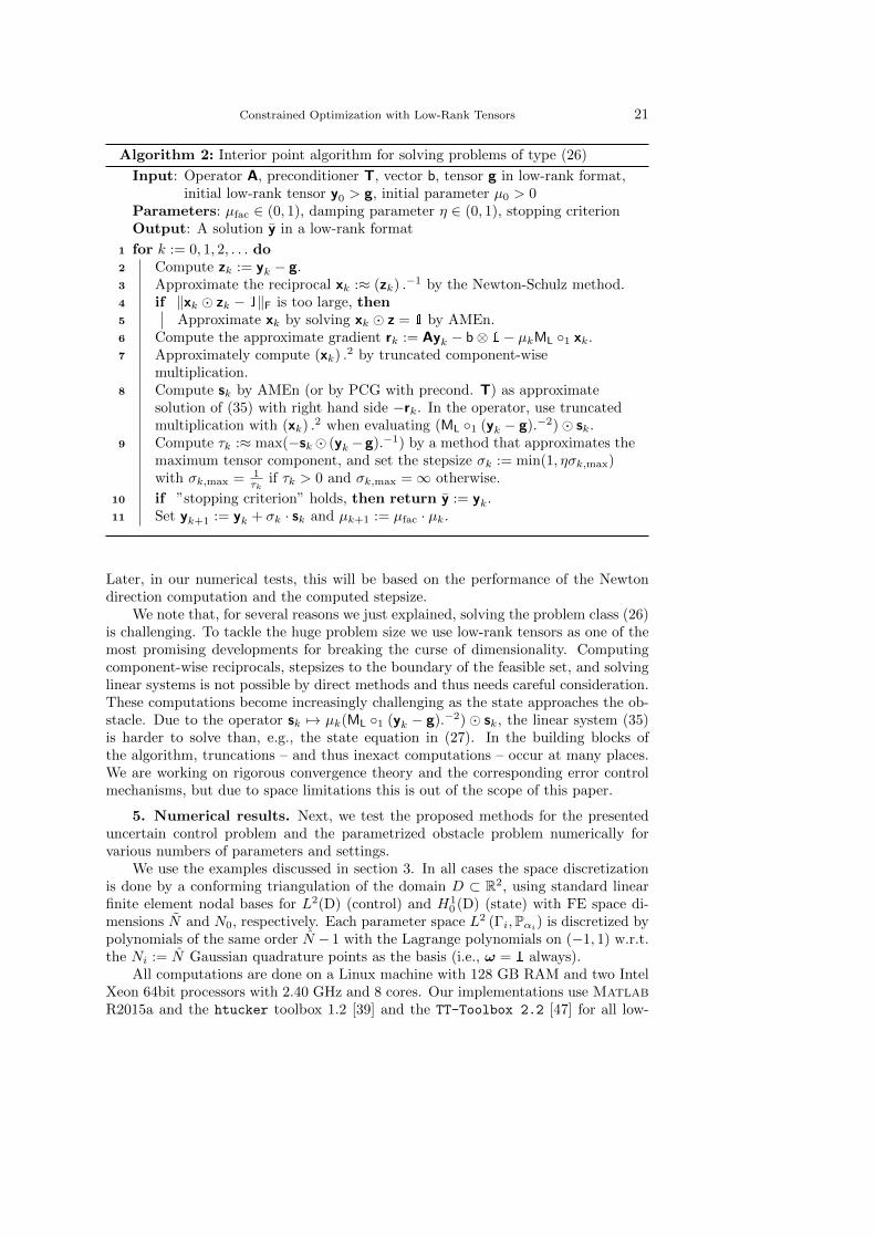
Algorithm 2: Interior point algorithm for solving problems of type (26)
Input: Operator A, preconditioner T, vector b, tensor g in low-rank format,initial low-rank tensor y0 > g, initial parameter µ0 > 0
Parameters: µfac ∈ (0, 1), damping parameter η ∈ (0, 1), stopping criterionOutput: A solution y in a low-rank format
1 for k := 0, 1, 2, . . . do2 Compute zk := yk − g.3 Approximate the reciprocal xk :≈ (zk) .−1 by the Newton-Schulz method.4 if ‖xk � zk − 1‖F is too large, then5 Approximate xk by solving xk � z = 1 by AMEn.6 Compute the approximate gradient rk := Ayk − b⊗ 1− µkML ◦1 xk.7 Approximately compute (xk) .2 by truncated component-wise
multiplication.8 Compute sk by AMEn (or by PCG with precond. T) as approximate
solution of (35) with right hand side −rk. In the operator, use truncatedmultiplication with (xk) .2 when evaluating (ML ◦1 (yk − g).−2)� sk.
9 Compute τk :≈ max(−sk� (yk−g).−1) by a method that approximates themaximum tensor component, and set the stepsize σk := min(1, ησk,max)with σk,max = 1
τkif τk > 0 and σk,max =∞ otherwise.
10 if ”stopping criterion” holds, then return y := yk.11 Set yk+1 := yk + σk · sk and µk+1 := µfac · µk.
Later, in our numerical tests, this will be based on the performance of the Newtondirection computation and the computed stepsize.
We note that, for several reasons we just explained, solving the problem class (26)is challenging. To tackle the huge problem size we use low-rank tensors as one of themost promising developments for breaking the curse of dimensionality. Computingcomponent-wise reciprocals, stepsizes to the boundary of the feasible set, and solvinglinear systems is not possible by direct methods and thus needs careful consideration.These computations become increasingly challenging as the state approaches the ob-stacle. Due to the operator sk 7→ µk(ML ◦1 (yk − g).−2) � sk, the linear system (35)is harder to solve than, e.g., the state equation in (27). In the building blocks ofthe algorithm, truncations – and thus inexact computations – occur at many places.We are working on rigorous convergence theory and the corresponding error controlmechanisms, but due to space limitations this is out of the scope of this paper.
5. Numerical results. Next, we test the proposed methods for the presenteduncertain control problem and the parametrized obstacle problem numerically forvarious numbers of parameters and settings.
We use the examples discussed in section 3. In all cases the space discretizationis done by a conforming triangulation of the domain D ⊂ R2, using standard linearfinite element nodal bases for L2(D) (control) and H1
0 (D) (state) with FE space di-mensions N and N0, respectively. Each parameter space L2 (Γi,Pαi) is discretized bypolynomials of the same order N − 1 with the Lagrange polynomials on (−1, 1) w.r.t.the Ni := N Gaussian quadrature points as the basis (i.e., ω = 1 always).
All computations are done on a Linux machine with 128 GB RAM and two IntelXeon 64bit processors with 2.40 GHz and 8 cores. Our implementations use MatlabR2015a and the htucker toolbox 1.2 [39] and the TT-Toolbox 2.2 [47] for all low-
22 S. Garreis and M. Ulbrich
-1 -0.5 0 0.5 1
-1
-0.5
0
0.5
1
Square with 5 uncertain subdomains
-1 -0.5 0 0.5 1
-1
-0.5
0
0.5
1
Square with 7 uncertain subdomains
-1 -0.5 0 0.5 1
-1
-0.5
0
0.5
1
Square with 9 uncertain subdomains
-1 -0.5 0 0.5 1
-1
-0.5
0
0.5
1
Square with 11 uncertain subdomains
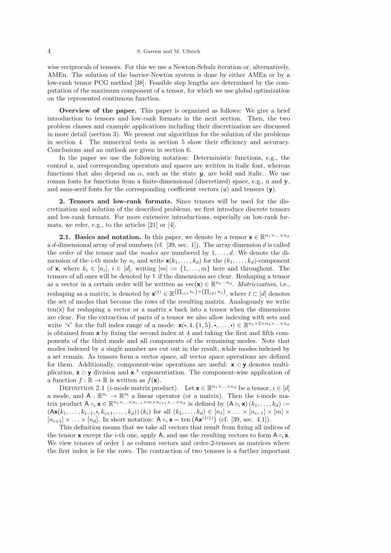
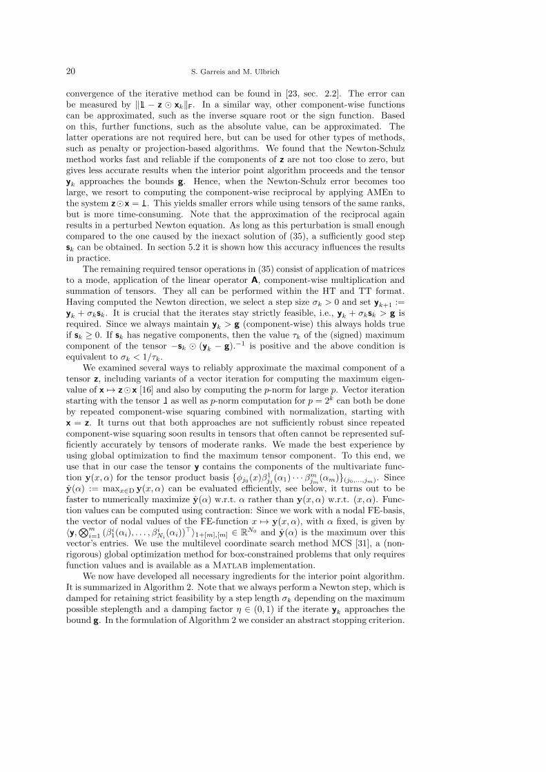
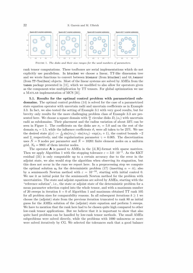
Figure 1. The disks and their size ranges for the used numbers of parameters.
rank tensor computations. These toolboxes are serial implementations which do notexplicitly use parallelism. In htucker we choose a linear, TT-like dimension treeand we wrote functions to convert between htensor (from htucker) and tt tensor
(from TT-Toolbox) objects. Most of the linear systems are solved by AMEn from thetamen package presented in [11], which we modified to also allow for operators givenas the component-wise multiplication by TT tensors. For global optimization we usea Matlab implementation of MCS [31].
5.1. Results for the optimal control problem with parametrized sub-domains. The optimal control problem (14) is solved for the case of a parametrizedstate equation operator with uncertain radii and uncertain coefficients as in Example3.3. In fact, we also tested the setting of Example 3.1 with very good results, but forbrevity only results for the more challenging problem class of Example 3.3 are pre-sented here. We choose a square domain with m
2 circular disks Di (αi) with uncertainradii as subdomains. Their placement and the radius variation of about 33% can beseen in Figure 1. The coefficients on the disks are σi = 5.0 and on the rest of thedomain σ0 = 1.5, while the influence coefficients ϑi were all taken to be 25%. We usethe desired state y(x) := 1
10 sin(πx1) · sin(πx2) · exp(x1 + 1), the control bounds −2and 2, respectively, and the regularization parameter γ = 0.005. The discretizationuses N = 9 nodes per parameter and N = 10201 finite element nodes on a uniformgrid, N0 = 9801 of them interior nodes.
The operator A is passed to AMEn in the {d,R}-format with sparse matrices.Then we apply Algorithm 1 with the stopping tolerance ε = 3.0 · 10−5. As the KKTresidual (31) is only computable up to a certain accuracy due to the error in theadjoint state, we also would stop the algorithm when observing its stagnation, butthis does not occur in the runs we report here. In a preprocessing step we computethe optimal solution u0 for the deterministic problem (17) (inserting α = α), alsoby a semismooth Newton method with ε = 10−10, starting with initial control 0.We use it as initial point for the semismooth Newton method for the problem withuncertainties. The state and adjoint equations are solved by AMEn, starting with the“reference solution”, i.e., the state or adjoint state of the deterministic problem for amean parameter selection copied into the whole tensor, and with a maximum numberof 20 sweeps in iteration k = 0 of Algorithm 1 and maximum obtained TT rank 105for all problem sizes for comparability reasons. In all subsequent iterations k ≥ 1 wechoose the (adjoint) state from the previous iteration truncated to rank 80 as initialguess for the AMEn solution of the (adjoint) state equation and perform 5 sweeps.We have to mention that the rank here had to be chosen quite high compared to otherlow-rank tensor applications. But we believe that it is important to show that alsoquite hard problems can be handled by low-rank tensor methods. The small AMEnsubproblems were solved directly, while the problems with 1000 unknowns or morewere solved iteratively by CG. We selected the tolerances such that a good balance
Constrained Optimization with Low-Rank Tensors 23
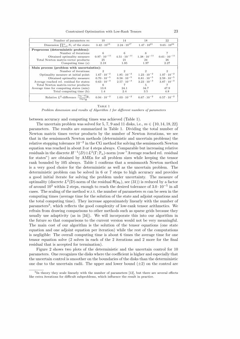
Number of parameters m: 10 14 18 22
Dimension∏mi=0 Ni of the state: 3.42 · 1013 2.24 · 1017 1.47 · 1021 9.65 · 1024
Preprocess (deterministic problem):Number of iterations: 6 6 6 7
Obtained optimality measure: 0.97 · 10−11 4.51 · 10−11 1.38 · 10−11 0.61 · 10−11
Total Newton matrix-vector products: 25 21 24 26Computing time (s): 2.18 1.85 1.97 2.27
Main process (problem with uncertainties):Number of iterations: 2 2 2 2
Optimality measure at initial point: 1.67 · 10−2 1.85 · 10−2 1.23 · 10−2 1.07 · 10−2
Obtained optimality measure: 0.70 · 10−5 0.58 · 10−5 0.81 · 10−5 2.59 · 10−5
Average reached rel. residual for states: 0.63 · 10−3 2.57 · 10−3 3.23 · 10−3 3.87 · 10−3
Total Newton matrix-vector products: 6 7 5 7Average time for computing states (min): 13.8 24.1 34.7 47.9
Total computing time (h): 1.4 2.4 3.5 4.8
Relative L2-difference‖u0−u‖
M‖u0‖M
: 0.94 · 10−2 1.03 · 10−2 0.67 · 10−2 0.57 · 10−2
Table 1Problem dimension and results of Algorithm 1 for different numbers of parameters
between accuracy and computing times was achieved (Table 1).The uncertain problem was solved for 5, 7, 9 and 11 disks, i.e., m ∈ {10, 14, 18, 22}
parameters. The results are summarized in Table 1. Dividing the total number ofNewton matrix times vector products by the number of Newton iterations, we seethat in the semismooth Newton methods (deterministic and uncertain problems) therelative stopping tolerance 10−2 in the CG method for solving the semismooth Newtonequation was reached in about 3 or 4 steps always. Comparable but increasing relativeresiduals in the discrete H−1(D)⊗L2(Γ;Pα)-norm (row ”Average reached rel. residualfor states”) are obtained by AMEn for all problem sizes while keeping the tensorrank bounded by 105 always. Table 1 confirms that a semismooth Newton methodis a very good choice for the deterministic as well as the uncertain problem. Thedeterministic problem can be solved in 6 or 7 steps to high accuracy and providesa good initial iterate for solving the problem under uncertainty. The measure ofoptimality (discrete L2(D)-norm of the residual R(uk), see (31)) is reduced by a factorof around 103 within 2 steps, enough to reach the desired tolerance of 3.0 · 10−5 in allcases. The scaling of the method w.r.t. the number of parameters m can be seen in thecomputing times (average time for the solution of the state and adjoint equations andthe total computing time). They increase approximately linearly with the number ofparameters5, which reflects the good complexity of low-rank tensor arithmetics. Werefrain from drawing comparisons to other methods such as sparse grids because theyusually use adaptivity (as in [34]). We will incorporate this into our algorithm inthe future so that comparisons to the current version would not be very meaningful.The main cost of our algorithm is the solution of the tensor equations (one stateequation and one adjoint equation per iteration) while the rest of the computationsis negligible: The overall computing time is about 6 times the average time for onetensor equation solve (2 solves in each of the 2 iterations and 2 more for the finalresidual that is accepted for termination).
Figure 2 shows two plots of the deterministic and the uncertain control for 10parameters. One recognizes the disks where the coefficient is higher and especially thatthe uncertain control is smoother on the boundaries of the disks than the deterministicone due to the uncertain radii. The upper and lower bound (±2) on the control are
5In theory they scale linearly with the number of parameters [12], but there are several effectslike extra iterations for difficult subproblems, which influence the result in practice.
24 S. Garreis and M. Ulbrich
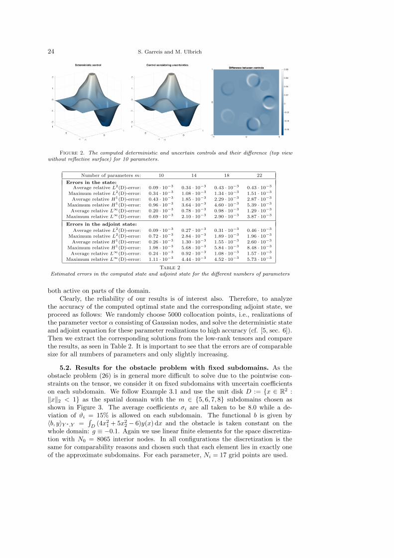
Figure 2. The computed deterministic and uncertain controls and their difference (top viewwithout reflective surface) for 10 parameters.
Number of parameters m: 10 14 18 22
Errors in the state:Average relative L2(D)-error: 0.09 · 10−3 0.34 · 10−3 0.43 · 10−3 0.43 · 10−3
Maximum relative L2(D)-error: 0.34 · 10−3 1.08 · 10−3 1.34 · 10−3 1.51 · 10−3
Average relative H1(D)-error: 0.43 · 10−3 1.85 · 10−3 2.29 · 10−3 2.87 · 10−3
Maximum relative H1(D)-error: 0.96 · 10−3 3.64 · 10−3 4.60 · 10−3 5.39 · 10−3
Average relative L∞(D)-error: 0.20 · 10−3 0.78 · 10−3 0.98 · 10−3 1.29 · 10−3
Maximum relative L∞(D)-error: 0.69 · 10−3 2.10 · 10−3 2.90 · 10−3 3.87 · 10−3
Errors in the adjoint state:
Average relative L2(D)-error: 0.09 · 10−3 0.27 · 10−3 0.31 · 10−3 0.46 · 10−3
Maximum relative L2(D)-error: 0.72 · 10−3 2.84 · 10−3 1.89 · 10−3 1.96 · 10−3
Average relative H1(D)-error: 0.26 · 10−3 1.30 · 10−3 1.55 · 10−3 2.60 · 10−3
Maximum relative H1(D)-error: 1.98 · 10−3 5.68 · 10−3 5.84 · 10−3 8.48 · 10−3
Average relative L∞(D)-error: 0.24 · 10−3 0.92 · 10−3 1.08 · 10−3 1.57 · 10−3
Maximum relative L∞(D)-error: 1.11 · 10−3 4.44 · 10−3 4.52 · 10−3 5.73 · 10−3
Table 2Estimated errors in the computed state and adjoint state for the different numbers of parameters
both active on parts of the domain.Clearly, the reliability of our results is of interest also. Therefore, to analyze
the accuracy of the computed optimal state and the corresponding adjoint state, weproceed as follows: We randomly choose 5000 collocation points, i.e., realizations ofthe parameter vector α consisting of Gaussian nodes, and solve the deterministic stateand adjoint equation for these parameter realizations to high accuracy (cf. [5, sec. 6]).Then we extract the corresponding solutions from the low-rank tensors and comparethe results, as seen in Table 2. It is important to see that the errors are of comparablesize for all numbers of parameters and only slightly increasing.
5.2. Results for the obstacle problem with fixed subdomains. As theobstacle problem (26) is in general more difficult to solve due to the pointwise con-straints on the tensor, we consider it on fixed subdomains with uncertain coefficientson each subdomain. We follow Example 3.1 and use the unit disk D := {x ∈ R2 :‖x‖2 < 1} as the spatial domain with the m ∈ {5, 6, 7, 8} subdomains chosen asshown in Figure 3. The average coefficients σi are all taken to be 8.0 while a de-viation of ϑi = 15% is allowed on each subdomain. The functional b is given by〈b, y〉Y ∗,Y =
∫D
(4x21 + 5x2
2 − 6)y(x) dx and the obstacle is taken constant on thewhole domain: g ≡ −0.1. Again we use linear finite elements for the space discretiza-tion with N0 = 8065 interior nodes. In all configurations the discretization is thesame for comparability reasons and chosen such that each element lies in exactly oneof the approximate subdomains. For each parameter, Ni = 17 grid points are used.
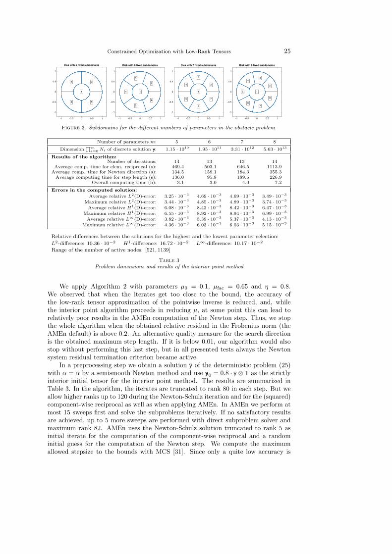
Constrained Optimization with Low-Rank Tensors 25
-1 -0.5 0 0.5 1
-1
-0.5
0
0.5
1
1
23
4 5
Disk with 5 fixed subdomains
-1 -0.5 0 0.5 1
-1
-0.5
0
0.5
1
1
2
3
4
5
6
Disk with 6 fixed subdomains
-1 -0.5 0 0.5 1
-1
-0.5
0
0.5
1
1
2
3
4
5
6
7
Disk with 7 fixed subdomains
-1 -0.5 0 0.5 1
-1
-0.5
0
0.5
1
1
2
34
5
67
8
Disk with 8 fixed subdomains
Figure 3. Subdomains for the different numbers of parameters in the obstacle problem.
Number of parameters m: 5 6 7 8
Dimension∏mi=0 Ni of discrete solution y: 1.15 · 1010 1.95 · 1011 3.31 · 1012 5.63 · 1013
Results of the algorithm:Number of iterations: 14 13 13 14
Average comp. time for elem. reciprocal (s): 469.4 503.1 646.5 1113.9Average comp. time for Newton direction (s): 134.5 158.1 184.3 355.3
Average computing time for step length (s): 136.0 95.8 189.5 226.9Overall computing time (h): 3.1 3.0 4.0 7.2
Errors in the computed solution:
Average relative L2(D)-error: 3.25 · 10−3 4.69 · 10−3 4.69 · 10−3 3.49 · 10−3
Maximum relative L2(D)-error: 3.44 · 10−3 4.85 · 10−3 4.89 · 10−3 3.74 · 10−3
Average relative H1(D)-error: 6.08 · 10−3 8.42 · 10−3 8.42 · 10−3 6.47 · 10−3
Maximum relative H1(D)-error: 6.55 · 10−3 8.92 · 10−3 8.94 · 10−3 6.99 · 10−3
Average relative L∞(D)-error: 3.82 · 10−3 5.39 · 10−3 5.37 · 10−3 4.13 · 10−3
Maximum relative L∞(D)-error: 4.36 · 10−3 6.03 · 10−3 6.03 · 10−3 5.15 · 10−3
Relative differences between the solutions for the highest and the lowest parameter selection:
L2-difference: 10.36 · 10−2 H1-difference: 16.72 · 10−2 L∞-difference: 10.17 · 10−2
Range of the number of active nodes: [521, 1139]
Table 3Problem dimensions and results of the interior point method
We apply Algorithm 2 with parameters µ0 = 0.1, µfac = 0.65 and η = 0.8.We observed that when the iterates get too close to the bound, the accuracy ofthe low-rank tensor approximation of the pointwise inverse is reduced, and, whilethe interior point algorithm proceeds in reducing µ, at some point this can lead torelatively poor results in the AMEn computation of the Newton step. Thus, we stopthe whole algorithm when the obtained relative residual in the Frobenius norm (theAMEn default) is above 0.2. An alternative quality measure for the search directionis the obtained maximum step length. If it is below 0.01, our algorithm would alsostop without performing this last step, but in all presented tests always the Newtonsystem residual termination criterion became active.
In a preprocessing step we obtain a solution y of the deterministic problem (25)with α = α by a semismooth Newton method and use y0 = 0.8 · y ⊗ 1 as the strictlyinterior initial tensor for the interior point method. The results are summarized inTable 3. In the algorithm, the iterates are truncated to rank 80 in each step. But weallow higher ranks up to 120 during the Newton-Schulz iteration and for the (squared)component-wise reciprocal as well as when applying AMEn. In AMEn we perform atmost 15 sweeps first and solve the subproblems iteratively. If no satisfactory resultsare achieved, up to 5 more sweeps are performed with direct subproblem solver andmaximum rank 82. AMEn uses the Newton-Schulz solution truncated to rank 5 asinitial iterate for the computation of the component-wise reciprocal and a randominitial guess for the computation of the Newton step. We compute the maximumallowed stepsize to the bounds with MCS [31]. Since only a quite low accuracy is
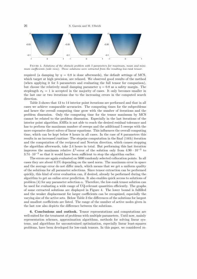
26 S. Garreis and M. Ulbrich
Figure 4. Solutions of the obstacle problem with 5 parameters for maximum, mean and mini-mum coefficients (side view). These solutions were extracted from the resulting low-rank tensor.
required (a damping by η = 0.8 is done afterwards), the default settings of MCS,which target at high precision, are relaxed. We observed good results of the method(when applying it for 5 parameters and evaluating the full tensor for comparison),but choose the relatively small damping parameter η = 0.8 as a safety margin. Thesteplength σk = 1 is accepted in the majority of cases. It only becomes smaller inthe last one or two iterations due to the increasing errors in the computed searchdirection.
Table 3 shows that 13 to 14 interior point iterations are performed and that in allcases we achieve comparable accuracies. The computing times for the subproblemsand hence the overall computing time grow with the number of iterations and theproblem dimension. Only the computing time for the tensor maximum by MCScannot be related to the problem dimension. Especially in the last iterations of theinterior point algorithm AMEn is not able to reach the desired residual tolerance andhas to perform the maximum number of sweeps and the additional 5 sweeps with themore expensive direct solves of linear equations. This influences the overall computingtime, which can be kept below 8 hours in all cases. In the case of 8 parameters thisresults in an increased runtime: The stepsize computation in the final (14th) iterationand the computation of the reciprocal and Newton direction, which causes stoppingthe algorithm afterwards, take 2.4 hours in total. But performing this last iterationimproves the maximum relative L2-error of the solution only from 4.90 · 10−3 to3.74 · 10−3 so that it would have been sufficient to stop the algorithm earlier.
The errors are again evaluated on 5000 randomly selected collocation points. In allcases they are about 0.5% depending on the used norm. The maximum error in spaceand the average error do not differ much, which means that we get a uniform qualityof the solutions for all parameter selections. Since tensor extraction can be performedquickly, this kind of error evaluation can, if desired, already be performed during thealgorithm to get an online error prediction. It also enables quick access to solutions ofproblem (4) for any parameter selection α. Therefore, the low-rank tensor solution canbe used for evaluating a wide range of UQ-relevant quantities efficiently. The graphsof some extracted solutions are displayed in Figure 4. The lower bound is fulfilledand the weaker displacement for larger coefficients can be recognized, especially thevarying size of the active sets. Below Table 3 the differences of the solutions for largestand smallest coefficients are listed. The range of the number of active nodes given inthe last row also depicts the difference between the solutions.
6. Conclusions and outlook. Tensor representations and computations arewell-suited for the treatment of problems with multiple parameters. Until now, mainlyrepresentation schemes, approximation algorithms, methods for solving linear sys-tems, and algorithms for unconstrained optimization, especially linear least-squaresproblems, have been developed for low-rank tensors. In this paper, we considered in-
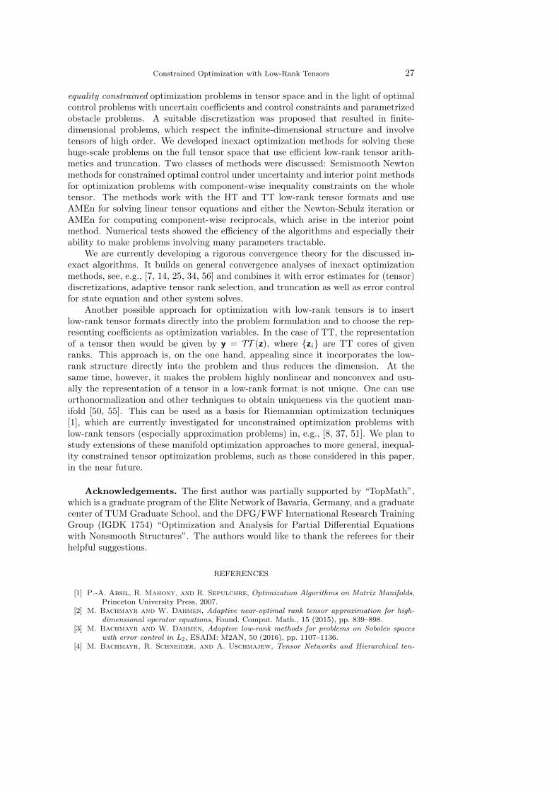
Constrained Optimization with Low-Rank Tensors 27
equality constrained optimization problems in tensor space and in the light of optimalcontrol problems with uncertain coefficients and control constraints and parametrizedobstacle problems. A suitable discretization was proposed that resulted in finite-dimensional problems, which respect the infinite-dimensional structure and involvetensors of high order. We developed inexact optimization methods for solving thesehuge-scale problems on the full tensor space that use efficient low-rank tensor arith-metics and truncation. Two classes of methods were discussed: Semismooth Newtonmethods for constrained optimal control under uncertainty and interior point methodsfor optimization problems with component-wise inequality constraints on the wholetensor. The methods work with the HT and TT low-rank tensor formats and useAMEn for solving linear tensor equations and either the Newton-Schulz iteration orAMEn for computing component-wise reciprocals, which arise in the interior pointmethod. Numerical tests showed the efficiency of the algorithms and especially theirability to make problems involving many parameters tractable.
We are currently developing a rigorous convergence theory for the discussed in-exact algorithms. It builds on general convergence analyses of inexact optimizationmethods, see, e.g., [7, 14, 25, 34, 56] and combines it with error estimates for (tensor)discretizations, adaptive tensor rank selection, and truncation as well as error controlfor state equation and other system solves.
Another possible approach for optimization with low-rank tensors is to insertlow-rank tensor formats directly into the problem formulation and to choose the rep-resenting coefficients as optimization variables. In the case of TT, the representationof a tensor then would be given by y = TT (z), where {zi} are TT cores of givenranks. This approach is, on the one hand, appealing since it incorporates the low-rank structure directly into the problem and thus reduces the dimension. At thesame time, however, it makes the problem highly nonlinear and nonconvex and usu-ally the representation of a tensor in a low-rank format is not unique. One can useorthonormalization and other techniques to obtain uniqueness via the quotient man-ifold [50, 55]. This can be used as a basis for Riemannian optimization techniques[1], which are currently investigated for unconstrained optimization problems withlow-rank tensors (especially approximation problems) in, e.g., [8, 37, 51]. We plan tostudy extensions of these manifold optimization approaches to more general, inequal-ity constrained tensor optimization problems, such as those considered in this paper,in the near future.
Acknowledgements. The first author was partially supported by “TopMath”,which is a graduate program of the Elite Network of Bavaria, Germany, and a graduatecenter of TUM Graduate School, and the DFG/FWF International Research TrainingGroup (IGDK 1754) “Optimization and Analysis for Partial Differential Equationswith Nonsmooth Structures”. The authors would like to thank the referees for theirhelpful suggestions.
REFERENCES
[1] P.-A. Absil, R. Mahony, and R. Sepulchre, Optimization Algorithms on Matrix Manifolds,Princeton University Press, 2007.
[2] M. Bachmayr and W. Dahmen, Adaptive near-optimal rank tensor approximation for high-dimensional operator equations, Found. Comput. Math., 15 (2015), pp. 839–898.
[3] M. Bachmayr and W. Dahmen, Adaptive low-rank methods for problems on Sobolev spaceswith error control in L2, ESAIM: M2AN, 50 (2016), pp. 1107–1136.
[4] M. Bachmayr, R. Schneider, and A. Uschmajew, Tensor Networks and Hierarchical ten-
28 S. Garreis and M. Ulbrich
sors for the Solution of High-dimensional Partial Differential Equations, Found. Comput.Math., (2016).
[5] J. Ballani and L. Grasedyck, Hierarchical tensor approximation of output quantities ofparameter-dependent PDEs, SIAM/ASA J. Uncertain. Quantif., 3 (2015), pp. 852–872.
[6] A. Barth, C. Schwab, and N. Zollinger, Multi-level Monte Carlo finite element method forelliptic PDEs with stochastic coefficients, Numer. Math., 119 (2011), pp. 123–161.
[7] S. Bellavia, Inexact interior-point method, J. Optim. Theory Appl., 96 (1998), pp. 109–121.[8] C. Da Silva and F. Herrmann, Optimization on the Hierarchical Tucker manifold – Appli-
cations to tensor completion, Linear Algebra Appl., 481 (2015), pp. 131–173.[9] L. de Lathauwer, B. de Moor, and J. Vandewalle, A multilinear singular value decompo-
sition, SIAM J. Matrix Anal. Appl., 21 (2000), pp. 1253–1278.[10] V. de Silva and L.-H. Lim, Tensor rank and the ill-posedness of the best low-rank approxima-
tion problem, SIAM J. Matrix Anal. Appl., 30 (2008), pp. 1084–1127.[11] S. V. Dolgov, Alternating minimal energy approach to ODEs and conservation laws in tensor
product formats. arXiv preprint 1403.8085, 2014.[12] S. V. Dolgov and D. V. Savostyanov, Alternating minimal energy methods for linear systems
in higher dimensions, SIAM J. Sci. Comput., 36 (2014), pp. A2248–A2271.[13] C. Eckardt and G. Young, The Approximation of one Matrix by Another of Lower Rank,
Psychometrika, 1 (1936).[14] S. C. Eisenstat and H. F. Walker, Globally convergent inexact Newton methods, SIAM J.
Optim., 19 (1994), pp. 393–422.[15] M. Espig, W. Hackbusch, A. Litvinenko, H. G. Matthies, and P. Wahnert, Efficient low-
rank approximation of the stochastic Galerkin matrix in tensor formats, Comput. Math.Appl., 67 (2014), pp. 818–829.
[16] M. Espig, W. Hackbusch, A. Litvinenko, H. G. Matthies, and E. Zander, Efficient analy-sis of high dimensional data in tensor formats, in Sparse Grids and Applications, J. Garckeand M. Griebel, eds., Springer-Verlag, 2013.
[17] A. Falco and A. Nouy, Proper generalized decomposition for nonlinear convex problems intensor Banach spaces, Numer. Math., 121 (2012), pp. 503–530.
[18] R. Forster and R. Kornhuber, A polynomial chaos approach to stochastic variational in-equalities, J. Numer. Math., 18 (2010), pp. 235–255.
[19] J. Garcke, Sparse grids in a nutshell, in Sparse Grids and Applications, J. Garcke andM. Griebel, eds., Springer-Verlag, 2013.
[20] L. Grasedyck, Hierarchical singular value decomposition of tensors, SIAM J. Matrix Anal.Appl., 31 (2010), pp. 2029–2054.
[21] L. Grasedyck, D. Kressner, and C. Tobler, A literature survey of low-rank tensor approx-imation techniques, GAMM-Mitt., 36 (2013), pp. 53–78.
[22] W. Hackbusch, Tensor Spaces and Numerical Tensor Calculus, Springer-Verlag, 2012.[23] W. Hackbusch, B. N. Khoromskij, and E. E. Tyrtyshnikov, Approximate iterations for
structured matrices, Numer. Math., 109 (2008), pp. 365–383.[24] W. Hackbusch and S. Kuhn, A new scheme for the tensor representation, J. Fourier Anal.
Appl., 15 (2009), pp. 706–722.[25] M. Heinkenschloss and L. N. Vicente, Analysis of inexact trust-region SQP algorithms,
SIAM J. Optim., 12 (2002), pp. 283–302.[26] M. Hintermuller, K. Ito, and K. Kunisch, The primal-dual active set strategy as a semis-
mooth Newton method, SIAM J. Optim., 13 (2002), pp. 865–888 (2003).[27] M. Hinze, R. Pinnau, M. Ulbrich, and S. Ulbrich, Optimization with PDE Constraints,
Springer, 2009.[28] Frank L. Hitchcock, The Expression of a Tensor or a Polyadic as a Sum of Products,
Journal of Mathematics and Physics, 6 (1927).[29] S. Holtz, T. Rohwedder, and R. Schneider, The alternating linear scheme for tensor opti-
mization in the tensor train format, SIAM J. Sci. Comput., 34 (2012), pp. A683–A713.[30] T. Huckle, K. Waldherr, and T. Schulte-Herbruggen, Computations in quantum tensor
networks, Linear Algebra Appl., (2012).[31] W. Huyer and A. Neumaier, Global optimization by multilevel coordinate search, J. Global
Optim., 14 (1999), pp. 331–355.[32] D. Kinderlehrer and G. Stampcchia, An Introduction to Variational Inequalities and their
Applications, SIAM, 2000.[33] T. G. Kolda and B. W. Bader, Tensor decompositions and applications, SIAM Rev., 51
(2009), pp. 455–500.[34] D. P. Kouri, M. Heinkenschloss, D. Ridzal, and B. G. van Bloemen Waanders, Inexact
objective function evaluations in a trust-region algorithm for PDE-constrained optimiza-
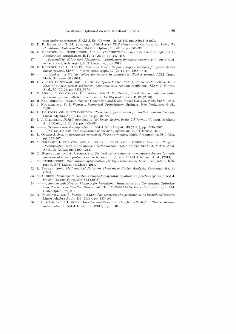
Constrained Optimization with Low-Rank Tensors 29
tion under uncertainty, SIAM J. Sci. Comput., 36 (2014), pp. A3011–A3029.[35] D. P. Kouri and T. M. Surowiec, Risk-Averse PDE-Constrained Optimization Using the
Conditional Value-at-Risk, SIAM J. Optim., 26 (2016), pp. 365–396.[36] D. Kressner, M. Steinlechner, and B. Vandereycken, Low-rank tensor completion by
Riemannian optimization, BIT, 54 (2014), pp. 447–468.[37] , Preconditioned low-rank Riemannian optimization for linear systems with tensor prod-
uct structure, tech. report, EPF Lausanne, July 2015.[38] D. Kressner and C. Tobler, Low-rank tensor Krylov subspace methods for parametrized
linear systems, SIAM J. Matrix Anal. Appl., 32 (2011), pp. 1288–1316.[39] , htucker – a Matlab toolbox for tensors in hierarchical Tucker format, ACM Trans.
Math. Software, 40 (2014).[40] F. Y. Kuo, C. Schwab, and I. H. Sloan, Quasi-Monte Carlo finite elements methods for a
class of elliptic partial differential equations with random coefficients, SIAM J. Numer.Anal., 50 (2012), pp. 3351–5574.
[41] V. Murg, F. Verstraete, O. Legeza, and R. M. Noack, Simulating strongly correlatedquantum systems with tree tensor networks, Physical Review B, 82 (2010).
[42] H. Niederreiter, Random Number Generation and Quasi-Monte Carlo Methods, SIAM, 1992.[43] J. Nocedal and S. J. Wright, Numerical Optimization, Springer, New York, second ed.,
2006.[44] I. Oseledets and E. Tyrtyshnikov, TT-cross approximation for multidimensional arrays,
Linear Algebra Appl., 432 (2010), pp. 70–88.[45] I. V. Oseledets, DMRG approach to fast linear algebra in the TT-format, Comput. Methods
Appl. Math., 11 (2011), pp. 382–393.[46] , Tensor-Train decomposition, SIAM J. Sci. Comput., 33 (2011), pp. 2295–2317.[47] , TT-toolbox 2.2: Fast multidimensional array operations in TT format, 2012.[48] L. Qi and J. Sun, A nonsmooth version of Newton’s method, Math. Progamming, 58 (1993),
pp. 353–367.[49] M. Sørensen, L. de Lathauwer, P. Comon, S. Icart, and L. Deneire, Canonical Polyadic
Decomposition with a Columnwise Orthonormal Factor Matrix, SIAM J. Matrix Anal.Appl., 33 (2012), pp. 1190–1213.
[50] T. Rohwedder and A. Uschmajew, On local convergence of alternating schemes for opti-mization of convex problems in the tensor train format, SIAM J. Numer. Anal., (2013).
[51] M. Steinlechner, Riemannian optimization for high-dimensional tensor completion, tech.report, EPF Lausanne, March 2015.
[52] L. Tucker, Some Mathematical Notes on Three-mode Factor Analysis, Psychometrika, 31(1966).
[53] M. Ulbrich, Semismooth Newton methods for operator equations in function spaces, SIAM J.Optim., 13 (2002), pp. 805–842 (2003).
[54] , Semismooth Newton Methods for Variational Inequalities and Constrained Optimiza-tion Problems in Function Spaces, vol. 11 of MOS-SIAM Series on Optimization, SIAM,Philadelphia, PA, 2011.
[55] A. Uschmajew and B. Vandereycken, The geometry of algorithms using hiearchical tensors,Linear Algebra Appl., 439 (2013), pp. 133–166.
[56] J. C. Ziems and S. Ulbrich, Adaptive multilevel inexact SQP methods for PDE-constrainedoptimization, SIAM J. Optim., 21 (2011), pp. 1–40.