constraining grace-derived cryosphere-attributed signal to ... · w. colgan et al.: constraining...

The Cryosphere, 7, 1901–1914, 2013www.the-cryosphere.net/7/1901/2013/doi:10.5194/tc-7-1901-2013© Author(s) 2013. CC Attribution 3.0 License.

The Cryosphere

Open A

ccess

Constraining GRACE-derived cryosphere-attributed signal toirregularly shaped ice-covered areas

W. Colgan1,2, S. Luthcke3, W. Abdalati1, and M. Citterio 2

1Cooperative Institute for Research in Environmental Sciences, University of Colorado, Boulder, CO, USA2Geological Survey of Denmark and Greenland, Copenhagen, Denmark3Goddard Space Flight Center, National Aeronautics and Space Administration, Greenbelt, MD, USA

Correspondence to:W. Colgan ([email protected])

Received: 18 April 2013 – Published in The Cryosphere Discuss.: 8 July 2013Revised: 4 November 2013 – Accepted: 13 November 2013 – Published: 17 December 2013

Abstract. We use a Monte Carlo approach to invert aspherical harmonic representation of cryosphere-attributedmass change in order to infer the most likely underlyingmass changes within irregularly shaped ice-covered areasat nominal 26 km resolution. By inverting a spherical har-monic representation through the incorporation of additionalfractional ice coverage information, this approach seeks toeliminate signal leakage between non-ice-covered and ice-covered areas. The spherical harmonic representation sug-gests a Greenland mass loss of 251± 25 Gt a−1 over theDecember 2003 to December 2010 period. The inversionsuggests 218± 20 Gt a−1 was due to the ice sheet proper,and 34± 5 Gt a−1 (or ∼ 14 %) was due to Greenland periph-eral glaciers and ice caps (GrPGICs). This mass loss fromGrPGICs exceeds that inferred from all ice masses on bothEllesmere and Devon islands combined. This partition there-fore highlights that GRACE-derived “Greenland” mass losscannot be taken as synonymous with “Greenland ice sheet”mass loss when making comparisons with estimates of icesheet mass balance derived from techniques that sample onlythe ice sheet proper.

1 Introduction

The Gravity Recovery And Climate Experiment (GRACE)satellite constellation measures anomalies in Earth’s gravityfield. Changes in ice sheet mass balance can be quantifiedthrough repeated observations of these gravitational anoma-lies. Unlike an altimetry approach (e.g., Zwally et al., 2011),in which an ice sheet volume change is converted into a mass

change, a gravimetry approach does not require the assump-tion of an effective density of change or an explicit treatmentof the refreezing versus runoff fraction of surface melt. Un-like an input–output approach (e.g., Rignot et al., 2008), inwhich interferometric synthetic aperture radar ice dischargeestimates are combined with modeled surface mass balanceestimates, a gravimetry approach does not require preciseknowledge of ice geometry or vertical velocity profiles neargrounding lines of outlet glaciers (Alley et al., 2007). Agravimetry approach to ice sheet mass balance, however, issensitive to the models used to isolate the cryospheric masschange signal from other signals, such as mass changes dueto land hydrology, ocean and atmospheric mass exchange andsolid earth processes. Several GRACE studies have docu-mented the increasingly negative mass balance of the Green-land ice sheet, from an initial estimate of−76± 26 Gt a−1

during the May 2002 to July 2004 period (Velicogna andWahr, 2005) to a more recent estimate of−263± 30 Gt a−1

during the January 2005 to December 2010 period (Shepherdet al., 2012).

GRACE-derived spherical harmonic solutions of rate ofmass change have coarse spatial resolution, and consequentlysignal leakage from within defined areas (Velicogna andWahr, 2006). While GRACE-derived mass change estimateshave been assessed at basin-scale resolution over the Green-land ice sheet (Luthcke et al., 2006; Velicogna and Wahr,2006; Sasgen et al., 2012; Barletta et al., 2013), signal leak-age has prevented the development of a GRACE-derivedmass change field that is completely constrained to withinthe irregularly shaped ice-covered areas of Greenland. De-constructing spherical harmonic solutions, in a non-iterative

Published by Copernicus Publications on behalf of the European Geosciences Union.

1902 W. Colgan et al.: Constraining GRACE signal to ice-covered areas

Fig. 1. (A) Cryosphere-attributed rate of mass change as GRACE mascons over the December 2003 to December 2010 period (Luthcke etal., 2013).(B) The equivalent spherical harmonic representation.

fashion using separate land and ocean filters, has beendemonstrated to reduce land–ocean signal leakage (Guo etal., 2010). The use of local mass concentrations (“mascons”)offers an alternative approach to improve spatial resolutionand reduce signal leakage (Luthcke et al., 2006; Jacob et al.,2012). No interpretation of satellite gravimetry, however, hasyet been capable of partitioning mass change due to Green-land peripheral glaciers and ice caps (GrPGICs) from thatdue to the Greenland ice sheet proper. It is desirable to isolateperipheral glacier mass change from ice sheet mass change,as it is believed that smaller peripheral glaciers and ice capsshould have shorter response times than the larger ice sheetto contemporary climate change (Nye, 1960; Jóhannesson etal., 1989).

2 Method

The fundamental problem addressed in this work is how toextract robust mass variations over spatially limited regionsfrom GRACE data (e.g., Simons et al., 2006). We use aMonte Carlo inversion to infer the most likely 26 km reso-lution rate of mass change field that, when smoothed witha Gaussian filter, closely reproduces a GRACE-observedspherical harmonic representation of cryosphere-attributedrate of mass change. This inversion of GRACE-observedrate of mass change incorporates new information in theform of observed fractional ice coverage. By constrainingthe inverted cryosphere-attributed rate of mass change to ice-covered areas, this approach seeks to eliminate signal leakagebetween non-ice-covered and ice-covered areas. We do not,however, purport to resolve spatial heterogeneity in rate ofmass change at the scale of individual glaciers and ice caps.Distinguishing sharp spatial heterogeneities in mass changesbetween adjacent ice-containing nodes would require the in-troduction of further new information to the inversion.

The variable notation used in the methodology descriptionis summarized in the Appendix Table A1.

2.1 Data

Our inversion requires two distinct input data: (i) a spher-ical harmonic representation of cryosphere-attributed rateof mass change, and (ii) glacier area/extent informationused to derive fractional ice coverage at a given node. Thespherical harmonic representation we invert characterizes thecryosphere-attributed rate of mass change over a given periodultimately derived from GRACE (MG), not individual spher-ical harmonic coefficients. We therefore invert a GRACE-derivedMG field in Cartesian space, rather than in sphericalharmonic space. Our time period of interest, over which theMG field is determined, is the 1 December 2003 to 1 De-cember 2010 GRACE inter-comparison period used by theIce Sheet Mass Balance Inter-comparison Exercise (IMBIE;Shepherd et al., 2012). TheMG field is derived by convertingtime series of cryosphere-attributed mascons into equivalentspherical harmonic solutions (Fig. 1).

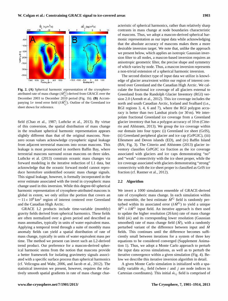
These mascons are derived from a NASA Goddard SpaceFlight Center (GSFC) data product in which GRACE level1 (L1) K band inter-satellite range rate (KBRR) data are re-duced via forward modeling into a series of iterated monthlymascons (Luthcke et al., 2013). During this L1 data re-duction, forward modeling and seasonal detrending removesmass changes associated with terrestrial hydrology, the oceanand atmosphere, as well as glacial isostatic adjustment andocean tides. Once these constraints have been applied inmascon space to limit leakage and isolate cryospheric masschange signal significantly, the linear mass change trend and1σ trend error are calculated for each mascon time series.Mascon-derived rates of mass change and associated errorare then converted into equivalent spherical harmonics of de-gree and order 60 (Fig. 2).

Mascons and spherical harmonics have been previouslydemonstrated to be interchangeable, essentially by represent-ing mascons as a set of differential potential coefficients(“delta coefficients”) added to the mean GRACE level 2 (L2)

The Cryosphere, 7, 1901–1914, 2013 www.the-cryosphere.net/7/1901/2013/

W. Colgan et al.: Constraining GRACE signal to ice-covered areas 1903

Fig. 2. (A) Spherical harmonic representation of the cryosphere-attributed rate of mass change (MG

ij) derived from GRACE over the

December 2003 to December 2010 period (Fig. 1b).(B) Accom-panying 1σ trend error field (δMG

ij). Outline of the Greenland ice

sheet shown for reference.

field (Chao et al., 1987; Luthcke et al., 2013). By virtueof this conversion, the spatial distribution of mass changein the resultant spherical harmonic representation appearsslightly different than that of the original mascons. Non-zero ocean values acknowledge cryospheric signal leakagefrom adjacent terrestrial mascons into ocean mascons. Thisleakage is most pronounced in northern Baffin Bay, whereterrestrial mascons surround ocean mascons on three sides.Luthcke et al. (2013) constrain oceanic mass changes viaforward modeling in the iterative reduction of L1 data, butacknowledge that the oceanic forward model cannot repro-duce heretofore unidentified oceanic mass change signals.This signal leakage, however, is formally incorporated in theerror estimate associated with the trend in cryospheric masschange used in this inversion. While this degree-60 sphericalharmonic representation of cryosphere-attributed mascons isglobal in extent, we only utilize the portion that covers an∼ 11× 106 km2 region of interest centered over Greenlandand the Canadian High Arctic.

GRACE L2 products include time-variable (monthly)gravity fields derived from spherical harmonics. These fieldsare often normalized over a given period and described asmass anomalies, typically in units of water equivalent mass.Applying a temporal trend through a suite of monthly massanomaly fields can yield a spatial distribution of rate ofmass change, typically in units of water equivalent mass pertime. The method we present can invert such an L2-derivedtrend product. Our preference for a mascon-derived spher-ical harmonic stems from the notion that mascons providea better framework for isolating gravimetry signals associ-ated with a specific surface process than spherical harmonics(cf. Velicogna and Wahr, 2006, and Jacob et al., 2012). Thestatistical inversion we present, however, requires the rela-tively smooth spatial gradients in rate of mass change char-

acteristic of spherical harmonics, rather than relatively sharpcontrasts in mass change at node boundaries characteristicof mascons. Thus, we adopt a mascon-derived spherical har-monic representation as our input data while acknowledgingthat the absolute accuracy of mascons makes them a moredesirable inversion target. We note that, unlike the approachwe present below, which applies an isotropic Gaussian inver-sion filter to all nodes, a mascon-based inversion requires ananisotropic geometric filter, the precise shape and symmetryof which varies by node. Thus, a mascon inversion representsa non-trivial extension of a spherical harmonic inversion.

The second distinct type of input data we utilize is knowl-edge of glacier area/extent within our region of interest cen-tered over Greenland and the Canadian High Arctic. We cal-culate the fractional ice coverage of all glaciers external toGreenland from the Randolph Glacier Inventory (RGI) ver-sion 2.0 (Arendt et al., 2012). This ice coverage includes thenorth and south Canadian Arctic, Iceland and Svalbard (i.e.,RGI regions 3, 4, 6 and 7), where the RGI polygon accu-racy is better than two Landsat pixels (or 30 m). We inter-polate fractional Greenland ice coverage from a Greenlandglacier inventory that has a polygon accuracy of 10 m (Citte-rio and Ahlstrøm, 2013). We group the ice coverage withinour domain into four types: (i) Greenland ice sheet (GrIS),(ii) Greenland peripheral glacier and ice cap (GrPGIC), (iii)Ellesmere and Devon islands (ED), and (iv) Baffin Island(BA; Fig. 3). The Citterio and Ahlstrøm (2013) glacier in-ventory classifies GrPGIC ice fraction as the ice coverageassociated with glaciers and ice caps demonstrating “no”and “weak” connectivity with the ice sheet proper, while theice coverage associated with glaciers demonstrating “strong”connectivity with the ice sheet proper is classified as GrIS icefraction (cf. Rastner et al., 2012).

2.2 Algorithm

We invert a 1000 simulation ensemble of GRACE-derivedrate of cryospheric mass change. In each simulation withinthe ensemble, the best estimateMG field is randomly per-turbed within its associated error (δMG) to yield a uniqueMG

+ δMG input field. An iterative approach is then usedto update the higher resolution (26 km) rate of mass changefield (m) and its corresponding lower resolution (Gaussiansmoothed) rate of mass change field (M), with a randomlyperturbed variant of the difference between input andM

fields. This continues until the difference becomes suffi-ciently small between iterations for a system of three keyequations to be considered converged (Supplement Anima-tion 1). Thus, we adopt a Monte Carlo approach to perturbthe input data across simulations, as well as to perturb theiterative convergence within a given simulation (Fig. 4). Be-low we describe this iterative inversion algorithm in detail.

A given Monte Carlo simulation is initialized with a spa-tially variable mij field (wherei andj are node indices inCartesian coordinates). This initialmij field is comprised of

www.the-cryosphere.net/7/1901/2013/ The Cryosphere, 7, 1901–1914, 2013


Fig. 3.Fractional ice coverage (Fij ) interpolated to 26 km by 26 km resolution:(A) Greenland ice sheet (GrIS; Citterio and Ahlstrøm, 2013),(B) Greenland’s peripheral glaciers and ice caps (GrPGICs; Citterio and Ahlstrøm, 2013), and(C) glaciers external to Greenland (Arendt etal., 2012). Boxes denote the ice coverage classified as Ellesmere and Devon islands (ED) and Baffin Island (BA).

Fig. 4.Flowchart overview of inverting a given lower (spherical har-monic) resolution GRACE-derived rate of mass change field (MG

ij)

into an ensemble of higher (26 km) resolution rate of mass changefields (mij ). An ensemble of 1000 simulations is performed, witheach simulation comprised of an iterative inversion to convergenceas defined by Eq. (5).

an array of random numbers uniformly distributed between−100 and+100 kg m−2 a−1 that has been multiplied by frac-tional ice area (Fij ). The initialmij field varies over the sameorder of magnitude as the anticipated finalmij field. Propor-tionately weighing the initialmij field by Fij allows a rea-sonable representation of uncertainty in the interior of theGreenland ice sheet (whereFij = 1) while also ensuring thatmij → 0 whereFij → 0. Given the relatively limited spatialextent of the inversion domain, and that non-ice-containingnodes constrained by boundary conditions completely sur-round the transient ice-containing nodes within the inversiondomain (Sect. 2.3), the final ensemble mean inversion is rel-atively insensitive to the choice of initial conditions over therange±0 to±100 kg m−2 a−1 (Sect. 4.1).

In each iteration, the Gaussian smoothed rate of masschange field (Mij ) is calculated by applying a fixed parame-ter Gaussian filter function (fG) to the inverted rate of masschange field (mij ):

Mkij = fG

(mk

ij ,σ), (1)

wherek denotes a given iteration, andσ is the prescribedcharacteristic scaling length (or standard deviation) of theisotropic Gaussian filter. While other filters, such as dataadaptive cosine windows, conserve more spherical harmoniclow-degree energy, thereby potentially allowing a more ac-curate description of spatial variability, we do not explorealternatives to the conventional Gaussian filter in this study(e.g., Longuevergne et al., 2010).

Relative to a given node, the spatial distribution of Gaus-sian filter weight across the inversion domain (Wij ; dimen-sionless) is described by

Wij =

(1

σ√

2π

)exp

(−d2

ij

2σ 2

), (2)

wheredij represents the distances between the given nodeand all nodes within the inversion domain. The numeratorunits in the above equation are implicitly the same as thoseof characteristic scaling length and inter-node distance (i.e.,“1 km” when σ and d are in km). Asdij and Wij are in-herently unique at each node, they are functionally three-dimensional arrays of the formdijp andWijp, wherep is aunique node coordinate ranging from 1 toi · j . Thus, apply-ing a Gaussian filter tomij in order to updateMij requireslooping through thep coordinate, from 1 toi · j , which is acomputationally expensive task.

We determine the optimum value ofσ through a sensitiv-ity analysis (Figs. 5 and 6). We invertm fields using char-acteristic Gaussian length scales of 150, 200 and 250 km.



Fig. 5. Ensemble mean inferred rate of mass change field (m) atice-containing nodes over nine sensitivity scenarios of various char-acteristic Gaussian smoothing lengths (σ) and non-ice-containingnode thresholdm values (mmax). Top row: σ = 150 km. Middlerow: σ = 200 km. Bottom row:σ = 250 km. Left column:mmax=

0 kg m−2 a−1. Middle column:mmax= 15 kg m−2 a−1. Right col-umn: mmax= 30 kg m−2 a−1. Black contour lines denote irregu-larly shaped ice-containing nodes within the domain. White contourlines denote 0 kg m−2 a−1.

We find that the root mean square (RMS) of the differ-ence field between the GRACE-derivedMG field and theGaussian smoothed inverted field (M) reaches a minimumwhenσ = 200 km, independent of prescribed boundary con-ditions described in Sect. 2.3 (Fig. 7). We therefore prescribea characteristic Gaussian length scale of 200 km in our in-version. The combination of a degree-60 spherical harmonicrepresentation and a characteristic Gaussian length scale of200 km should preserve maximum information of the mag-nitude and spatial distribution of mass changes through theinversion process while honoring the fundamental spatial res-olution of the GRACE satellites.

Fig. 6. Ensemble mean difference betweenMG and M (1)over nine sensitivity scenarios of various characteristic Gaussiansmoothing lengths (σ) and non-ice-containing node thresholdm

values (mmax). Top row: σ = 150 km. Middle row:σ = 200 km.Bottom row: σ = 250 km. Left column:mmax= 0 kg m−2 a−1.Middle column: mmax= 15 kg m−2 a−1. Right column:mmax=

30 kg m−2 a−1. Black contour lines denote irregularly shaped ice-containing nodes within the domain.

In a given iteration, the difference between the GRACE-derived rate of mass change and the Gaussian smoothed in-verted rate of mass change fields, denoted1k

ij , is determinedas

1kij =

(MG

ij + δMGij R

)− Mk

ij , (3)

whereδMGij R represents a perturbation of the input GRACE

solution (MGij ) within its associated 1σ error field, andMk

ij

represents the Gaussian smoothedmkij field in a given it-

eration. In each simulationR is a random scalar derivedfrom a normal distribution centered on zero with a standarddeviation of one.R varies across simulations, but is con-stant throughout the iterations of a given simulation. Over



Fig. 7.Root mean square (RMS) of theMG−M difference field (1;

Fig. 6) vs. characteristic Gaussian smoothing length (σ), for threedifferent non-ice-containing node thresholdm values (mmax).

an ensemble of simulations, any given region (or ice type)is thus inverted under relatively high and low initial rates ofmass change.

The preceding difference field is used to inform themij

field of the subsequent iteration according to

mk+1ij = mk

ij + 1kijR

kijFij , (4)

whereRkij is a spatially variable array of random values be-

tween 0 and 1, andFij is observed fractional ice coverageat a given node. In contrast to the scalarR used to perturbEq. (3), the arrayRk

ij is continually being repopulated byrandom numbers throughout the iterations of a given simu-lation (i.e.,Rij is not constant throughout the iterations of agiven simulation). Over a large number of iterations, a givennode is thus perturbed with relatively high and low1 valuesduring convergence towards a finalm value.

Local mascon rates of mass change derived from GRACEare known to be sensitive to the a priori imposition of prede-fined patterns of mass change (Horwath and Dietrich, 2009).This is not an issue with the mascon solution used here, how-ever, as Luthcke et al. (2013) derive mass changes from therigorous reduction of the KBRR residuals. In the context ofinverting the spherical harmonic representation, employing arandom number field in each iteration not only ensures thatinferred rates of mass change are not required to be spatiallycorrelated (i.e., subject to a prescribed covariance matrix),but actually enhances the algorithm ability to explore the in-finite number of possible solutions efficiently (e.g., Colganet al., 2012).

Introducing fractional ice coverage information in thefashion of Eq. (4) forces cryospheric rates of mass changeto be proportional with the fractional ice coverage at a givennode, rather than restricting inferred rates of mass changeto a binary field of non-ice-covered and ice-covered nodes(e.g., Barletta et al., 2013). For example, 10 times more masschange is attributed to a node withF = 1.0 than a neighbor-ing node withF = 0.1. While in reality specific mass loss(i.e., mass loss per unit ice-covered area) typically increasesto a maximum at the peripheral nodes of ice masses, incor-

Fig. 8. The system of equations in each simulation is deemed con-verged when the inferred total rate of mass change over all Green-land ice coverage (both GrIS and GrPGIC) varies by less than0.1 Gt a−1 between iterations (Eq. 5). The whisker plot at the rightshows one (thick line) and two (thin line) standard deviations fromthe ensemble mean.

porating an additional piece of new information would be re-quired in order to distinguish sharp contrasts in mass changebetween adjacent ice-containing nodes.

We iterate themij field by cycling through Eqs. (1)–(4)until the following condition is satisfied across all GrIS andGrPGIC nodes (Animation 1):∑

ij

(|mk+1

ij − mkij |Aij

)≤ 0.1Gta−1, (5)

whereAij is node area. We therefore deem the system ofequations as converged when the total rate of mass changeover all Greenland ice varies by less than 0.1 Gt a−1 betweeniterations. This typically takes between 75 to 100 iterationsper simulation, depending on prescribedσ value (Fig. 8). Weperform 1000 simulations in order to compute a robust en-semble meanmij field.

2.3 Boundary conditions

Here we describe the boundary conditions imposed at non-ice-containing nodes. By employing a spherical harmonicrepresentation that isolates the mass change associated withterrestrial ice, the mass changes associated with non-ice-containing nodes (whereF = 0) are theoretically negligi-ble (i.e.,m =0 kg m−2 a−1) . In practice, the mass changesat these non-ice-containing nodes are not truly zero, butrather within uncertainty of zero. We therefore perform asensitivity study in which we allowmij values at non-ice-containing nodes to vary below prescribed absolute thresholdvalues of 0, 15 or 30 kg m−2 a−1 (Figs. 5 and 6). A thresh-old of 0 kg m−2 a−1, for example, corresponds to the the-oretical expectation of no error in, or perfect isolation of,the cryospheric mass change signal. In comparison to de-termining the optimal characteristic Gaussian length scale(σ ) via an analogous sensitivity analysis, selecting whichnon-ice-containing nodemij threshold to implement is more



subjective. The RMS of the difference field between theGRACE-derivedMG field and the Gaussian smoothed in-verted field (M) decreases as the non-ice-containing nodemij threshold increases. RMS would ultimately go to zerowhen themij values permitted at non-ice-containing nodesare indistinguishable from those at ice-containing nodes(Fig. 7).

We therefore arbitrarily prescribe an absolute threshold(mmax) of 15 kg m−2 a−1 at non-ice-containing nodes. Thisboundary condition acknowledges a level of uncertainty inthe rate of mass change at non-ice-containing nodes thatis representative of the uncertainty typically assessed forGRACE-derived cryosphere-attributed spherical harmonicsolutions (Velicogna and Wahr, 2005; Longuevergne et al.,2010), and an order of magnitude less than themij values in-ferred by our Monte Carlo inversion approach at adjacent ice-containing nodes. This boundary condition is implemented atnon-ice-containing nodes according to

mk+1ij =

{mk

ij + 1kijR

kij if |mk

ij | < mmax

mmax if |mkij | ≥ mmax

}. (6)

This modified version of Eq. (4) is invoked at non-ice-containing nodes by a Heaviside, or unit step, function (Hij )of the following form (e.g., Colgan et al., 2012):

Hij =

{1 for Fij = 00 for Fij > 0

}. (7)

2.4 Domain

Here we describe the grid spacing and extent of our inver-sion domain. In the US National Snow and Ice Data Center(NSIDC) polar stereographic projection, our inversion do-main extends from−1625 km in the west to 1300 km in theeast, and from−125 km in the north to−3800 km in thesouth. This places the domain boundaries at least one char-acteristic Gaussian length scale from all major ice masses inGreenland and the Canadian Arctic Archipelago. There is aninherent trade-off between computational burden and hori-zontal grid resolution, as the former exponentially increasesas the latter linearly decreases. We prescribe a uniform gridspacing of 26 km, which results in 113 computational nodesalong the easting axis and 142 computational nodes alongthe northing axis, for a total of 16 046 computational nodeswithin the model domain.

While grid spacing is a uniform 26 km throughout ourdomain, the polar stereographic projection inherently intro-duces increasing distortion away from its central meridian(45◦ W) and parallel (70◦ N), which influences area calcula-tions. To compensate for area distortion, we use the true areaof each individual node across the domain (Aij ) in our cal-culations. Thus, while our nominal node area is 262 km2, thetrue areas of ice-containing nodes vary between 24.52 and27.52 km2 over the domain. 26 km is the minimum resolution

Fig. 9. The uncertainty in rate of mass change at any given ice-containing nodeij (δmij ) is taken as one standard deviation of thegiven node rate of mass change values across the ensemble of 1000simulations.

that allowsdijp to be stored as a single three-dimensional ar-ray (i · j · p = 113· 142· 16 046 elements) on the per proces-sor RAM allotment of JANUS supercomputer high memorynodes. This avoids recalculating the individual 113 by 142dij array associated with each of the 16 046 computationalnodes in each iteration. Each of the 1000 simulations withinan ensemble takes 181± 17 processor seconds on a 2.8 GHzcore with 12 GB of RAM on the University of Colorado’sJANUS supercomputer.

2.5 Partitioning mass change and uncertainty

Here we describe how the rate of mass change, and corre-sponding uncertainty, for each of the four ice types definedin Sect. 2.1 (GrIS, GrPGIC, ED and BA) is derived from theinvertedm field. By constraining inferred mass changes onlyto occur at ice-containing nodes, mass changes may be par-titioned amongst the distinct ice types within the inversiondomain. As nodes containing ED or BA ice type are geo-graphically separate from nodes containing other ice types,the total rate of mass change associated with ED or BA icetype may be quantified via a straightforward summation ofthe individual rates of mass change at all nodes of either icetype. In contrast, GrIS and GrPGIC ice types can coexist atthe same node; the areas of many nodes around the periph-ery of the Greenland ice sheet are partly covered by both icesheet and peripheral glaciers. When attributing rates of masschange to either GrIS or GrPGIC ice type at nodes shared byboth ice types, we weight attributable rates of mass changeby the fractional ice coverage of each ice type. For example,



Fig. 10. (A) Ensemble mean inferred rate of mass change field (m) at ice-containing nodes. Grey shading denotes non-ice-containing nodesand the white contour line denotes 0 kg m−2 a−1. (B) Gaussian smoothing (σ = 200 km) of the ensemble mean inferred rate of mass changefield (M). (C) Spherical harmonic representation of the trend in GRACE-derived cryosphere-attributed rate of mass change (MG). (D)Difference betweenMG andM (1). Black contour lines denote irregularly shaped ice-containing nodes within the domain.

the total rate of mass change for GrIS (∑

mGrIS) is summedas∑

mGrIS=

∑ij

(mij ·

F GrISij

F GrPGICij + F GrIS

ij

)Aij , (8)

whereAij is again an array of node true areas, and the super-script denotes GrPGIC and GrIS ice types. While the rates ofmass change contributions of GrIS and GrPGIC ice types at agiven node are indistinguishable to the inversion algorithm,in that they contribute to inferred mass change in the sameway, Eq. (8) provides a framework for statistically partition-ing ice sheet and peripheral glacier mass change at commonnodes. Given the historical expectation that smaller periph-eral glaciers and ice caps should have shorter response timesthan the larger ice sheet to contemporary climate change(Nye, 1960; Jóhannesson et al., 1989), this assumption mayunderestimate the true contribution of GrPGIC ice type tothe inferred mass change at a given node. Simply put, theGrPGIC : GrIS mass change at a given node likely exceedsthe GrPGIC : GrIS ice coverage.

After partitioning rates of mass change between distinctice types, it is desirable to quantify the uncertainty associatedwith the rate of mass change inferred for each ice type. Previ-ous glaciological applications of Monte Carlo inversion, suchas inferring basal sliding velocity from input data of surfacevelocity observations (e.g., Chandler et al., 2006), and in-ferring past surface temperature history from input data ofborehole temperature profiles (e.g., Muto et al., 2011), haveused the perturbation of input data within their associated un-certainty subsequently to estimate uncertainty in the invertedfield. We similarly take uncertainty inm at any given nodeij

(δmij ) as one standard deviation of the given nodemij valuesacross the ensemble of simulations (Fig. 9). As values of en-semble meanδmij are spatially correlated, we do not derivethe uncertainty in the rate of mass change of a given ice typefrom the point uncertainties of that ice type, but rather fromthe total rate of mass change of the given ice type across theensemble of inversions. We take uncertainty in the total rateof mass change of each ice type of interest (GrIS, GrPGIC,ED and BA) as one standard deviation in the total rate ofmass change of each ice type across the ensemble of 1000simulations.

3 Results

The ensemble mean Gaussian smoothed rate of mass changefield closely reproduces the spherical harmonic representa-tion of cryosphere-attributed mascons derived from GRACEobservations (Fig. 10). Both the observed and ensemblemean simulated fields exhibit similar patterns of Greenlandmass loss, extending from the Geikie Plateau in East Green-land around South Greenland to Humboldt Glacier in North-west Greenland, as well as mass gain focused in north centralGreenland. The difference between the finalM field and theinput MG field (1) is < 5 % of the absolute magnitude of theMG field throughout the vast majority of the inversion do-main. The largest discrepancy occurs in northern Baffin Bay,where the pattern of the spherical harmonic representationover the ocean infers more mass loss than is permitted bythe inversion parameters employed, resulting in a local max-imum in absolute discrepancy.



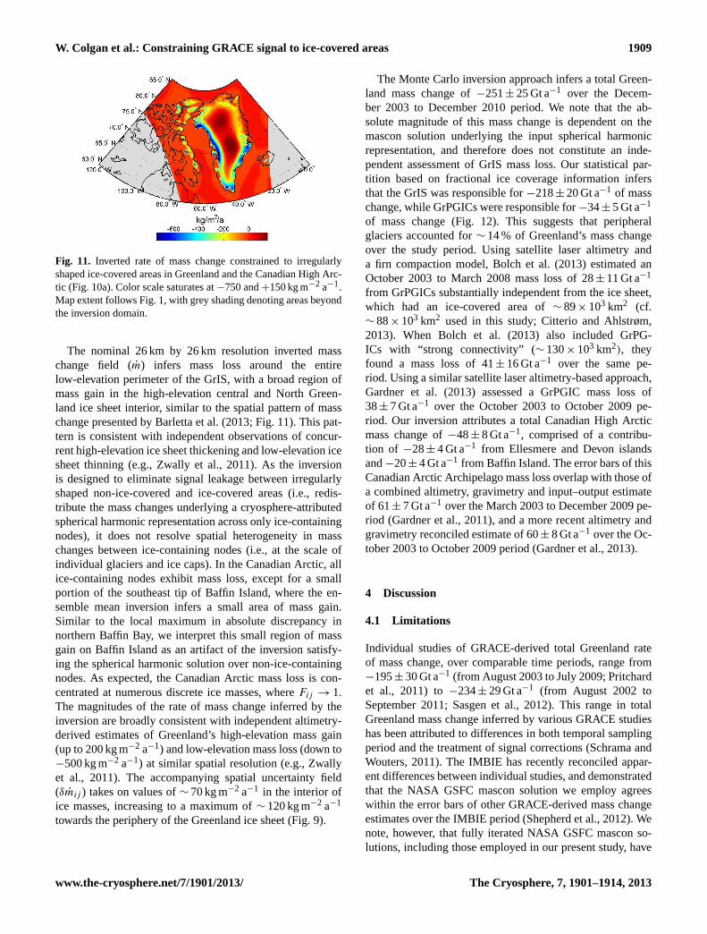
Fig. 11. Inverted rate of mass change constrained to irregularlyshaped ice-covered areas in Greenland and the Canadian High Arc-tic (Fig. 10a). Color scale saturates at−750 and+150 kg m−2 a−1.Map extent follows Fig. 1, with grey shading denoting areas beyondthe inversion domain.

The nominal 26 km by 26 km resolution inverted masschange field (m) infers mass loss around the entirelow-elevation perimeter of the GrIS, with a broad region ofmass gain in the high-elevation central and North Green-land ice sheet interior, similar to the spatial pattern of masschange presented by Barletta et al. (2013; Fig. 11). This pat-tern is consistent with independent observations of concur-rent high-elevation ice sheet thickening and low-elevation icesheet thinning (e.g., Zwally et al., 2011). As the inversionis designed to eliminate signal leakage between irregularlyshaped non-ice-covered and ice-covered areas (i.e., redis-tribute the mass changes underlying a cryosphere-attributedspherical harmonic representation across only ice-containingnodes), it does not resolve spatial heterogeneity in masschanges between ice-containing nodes (i.e., at the scale ofindividual glaciers and ice caps). In the Canadian Arctic, allice-containing nodes exhibit mass loss, except for a smallportion of the southeast tip of Baffin Island, where the en-semble mean inversion infers a small area of mass gain.Similar to the local maximum in absolute discrepancy innorthern Baffin Bay, we interpret this small region of massgain on Baffin Island as an artifact of the inversion satisfy-ing the spherical harmonic solution over non-ice-containingnodes. As expected, the Canadian Arctic mass loss is con-centrated at numerous discrete ice masses, whereFij → 1.The magnitudes of the rate of mass change inferred by theinversion are broadly consistent with independent altimetry-derived estimates of Greenland’s high-elevation mass gain(up to 200 kg m−2 a−1) and low-elevation mass loss (down to−500 kg m−2 a−1) at similar spatial resolution (e.g., Zwallyet al., 2011). The accompanying spatial uncertainty field(δmij ) takes on values of∼ 70 kg m−2 a−1 in the interior ofice masses, increasing to a maximum of∼ 120 kg m−2 a−1

towards the periphery of the Greenland ice sheet (Fig. 9).

The Monte Carlo inversion approach infers a total Green-land mass change of−251± 25 Gt a−1 over the Decem-ber 2003 to December 2010 period. We note that the ab-solute magnitude of this mass change is dependent on themascon solution underlying the input spherical harmonicrepresentation, and therefore does not constitute an inde-pendent assessment of GrIS mass loss. Our statistical par-tition based on fractional ice coverage information infersthat the GrIS was responsible for−218± 20 Gt a−1 of masschange, while GrPGICs were responsible for−34± 5 Gt a−1

of mass change (Fig. 12). This suggests that peripheralglaciers accounted for∼ 14 % of Greenland’s mass changeover the study period. Using satellite laser altimetry anda firn compaction model, Bolch et al. (2013) estimated anOctober 2003 to March 2008 mass loss of 28± 11 Gt a−1

from GrPGICs substantially independent from the ice sheet,which had an ice-covered area of∼ 89× 103 km2 (cf.∼ 88× 103 km2 used in this study; Citterio and Ahlstrøm,2013). When Bolch et al. (2013) also included GrPG-ICs with “strong connectivity” (∼ 130× 103 km2), theyfound a mass loss of 41± 16 Gt a−1 over the same pe-riod. Using a similar satellite laser altimetry-based approach,Gardner et al. (2013) assessed a GrPGIC mass loss of38± 7 Gt a−1 over the October 2003 to October 2009 pe-riod. Our inversion attributes a total Canadian High Arcticmass change of−48± 8 Gt a−1, comprised of a contribu-tion of −28± 4 Gt a−1 from Ellesmere and Devon islandsand−20± 4 Gt a−1 from Baffin Island. The error bars of thisCanadian Arctic Archipelago mass loss overlap with those ofa combined altimetry, gravimetry and input–output estimateof 61± 7 Gt a−1 over the March 2003 to December 2009 pe-riod (Gardner et al., 2011), and a more recent altimetry andgravimetry reconciled estimate of 60± 8 Gt a−1 over the Oc-tober 2003 to October 2009 period (Gardner et al., 2013).

4 Discussion

4.1 Limitations

Individual studies of GRACE-derived total Greenland rateof mass change, over comparable time periods, range from−195± 30 Gt a−1 (from August 2003 to July 2009; Pritchardet al., 2011) to−234± 29 Gt a−1 (from August 2002 toSeptember 2011; Sasgen et al., 2012). This range in totalGreenland mass change inferred by various GRACE studieshas been attributed to differences in both temporal samplingperiod and the treatment of signal corrections (Schrama andWouters, 2011). The IMBIE has recently reconciled appar-ent differences between individual studies, and demonstratedthat the NASA GSFC mascon solution we employ agreeswithin the error bars of other GRACE-derived mass changeestimates over the IMBIE period (Shepherd et al., 2012). Wenote, however, that fully iterated NASA GSFC mascon so-lutions, including those employed in our present study, have



Fig. 12. Ensemble probability density functions of rate of masschange inferred by Monte Carlo inversion over the Greenland icesheet (GrIS), Greenland peripheral glaciers and ice caps (GrPGICs),Ellesmere and Devon islands (ED) and Baffin Island (BA) over theDecember 2003 to December 2010 period.

been shown to produce greater mass loss values in compari-son to non-iterated NASA GSFC mascon solutions (Luthckeet al., 2013). We therefore acknowledge that initializing theMonte Carlo inversion with a different spherical harmonicrepresentation would yield a different inferred mass loss dis-tribution. Recognizing this limitation, we contend that ourpresent study demonstrates the utility of combining sphericalharmonics with additional information in the form of frac-tional ice coverage. By explicitly constraining cryosphere-attributed mass changes to irregularly shaped ice-covered ar-eas, we purport to have completely eliminated signal leakagebetween non-ice-covered and ice-covered areas.

GRACE mascons are conventionally expressed in units ofwater equivalent thickness per time, under the implicit as-sumption ofF = 1 at all nodes containing terrestrial ice mass(e.g., Barletta et al., 2013). We note that the cryosphere-attributed mass changeper unit areawe describe (mij ) is notequivalent to specificmij (i.e., cryosphere-attributed masschangeper unit ice-covered area). We may derive equiva-lent specificmij by dividing mij by Fij (Fig. 13). The rel-atively smooth gradients in the specificmij field are con-strained by the fundamental resolution of the GRACE satel-lites. While true specific mass loss typically increases to amaximum at the peripheral nodes of ice masses, the inver-sion we present would need a secondary piece of indepen-dent information in order to distinguish sharp contrasts inmass change between adjacent ice-containing nodes. Sincefractional ice coverage is the only new information we applyto GRACE data, the inversion only constrains cryosphere-attributed mass changes to ice-covered areas, and is not ca-pable of distinguishing spatial heterogeneity in mass loss be-tween adjacent ice-containing nodes. Altimetry data wouldbe a logical second piece of independent information to in-corporate, in order to distinguish differential rates of masschange between adjacent ice-containing nodes.

Fig. 13.Specific rate of cryospheric mass change per unit ice area(mij divided byFij ).

Finally, the precise role of initial conditions in inter-preting inferred mass changes is not entirely clear. As asensitivity test, we initialized the algorithm with a spa-tially uniform mij field of 0 kg m−2 a−1, rather than withrandom numbers uniformly distributed between−100 and+100 kg m−2 a−1 times fractional ice coverage. Under theserevised initial conditions, an ensemble of 1000 simulationsproduces a virtually identical total Greenland mass loss(250± 26 Gt a−1) and spatial pattern (not shown here, butavailable in Colgan et al., 2013). While total Greenland massloss is therefore insensitive to initial conditions over therange±0 to ±100 kg m−2 a−1, the spatial uncertainty fielddoes appear to be sensitive to selection of initial conditions.When mass changes are initialized with zeros, local uncer-tainty approaches zero in the high-elevation ice sheet interior(Fig. 14). Thus, deriving both ice-sheet-wide and local uncer-tainties from ensemble spread at convergence is not valid un-der all initial conditions, as ensemble spread is demonstrablydependent on choice of initial conditions. We contend that byimposing initial conditions that vary over the same order ofmagnitude as the anticipated inversion field, we have mini-mized the potential influence of initial condition hysteresis.We acknowledge, however, that we do not yet sufficientlyunderstand the behavior of this approach to encourage otherresearchers to blindly apply analogous inversions in differentcontexts. Application of Monte Carlo-type inversion to anysystem requires a deliberate selection of initial and boundaryconditions characteristic of the system under consideration.



Fig. 14.Sensitivity analysis of the spatial distribution of uncertainty in inferred mass changes (δmij ). (A) Uncertainty at a given node when

the inversion is initialized with a constant array of 0 kg m−2 a−1. (B) Uncertainty at a given node when the inversion is initialized with anarray of random numbers uniformly distributed between−100 and+100 kg m−2 a−1 times fractional ice coverage (identical to Fig. 9).(C) Difference.

4.2 Implications

The recent global mass loss trend of small glaciers and icecaps external to Greenland and Antarctica has been estimatedas between 148± 30 Gt a−1 (over January 2003 to Decem-ber 2010; Jacob et al., 2012) and 215± 26 Gt a−1 (over Oc-tober 2003 to October 2009; Gardner et al., 2013). Our es-timate of GrPGIC mass change over a similar period is be-tween∼ 16 and 23 % of these values. Projecting the futuresea level rise contribution of peripheral glaciers in Green-land and Antarctica, the 2007 Intergovernmental Panel onClimate Change report that “the global [glaciers and ice caps]sea level contribution [was] increased by a factor of 1.2 toinclude [peripheral glaciers] in Greenland and Antarctica”(Meehl et al., 2007). Our results suggest a comparable factor(e.g.,∼ 1.2) would be required to account for GrPGICs alonewhen using this scaling technique. We regard our GrPGICcontribution as a lower bound, however, due to (i) the po-tential underestimation of GrPGIC ice extent. The data setof Greenland ice sheet and peripheral glaciers we employ(Citterio and Ahlstrøm, 2013) does not classify as a GrPGICthose glaciers demonstrating “strong” connectivity with theice sheet proper (e.g., Geikie Plateau or Julianehåb Ice Cap;cf. Rastner et al., 2012), and may therefore be regarded as aconservative estimate of GrPGIC extent. (ii) There is an im-plicit assumption that mass changes are equally weighted be-tween GrIS and GrPGIC ice at common nodes (Eq. 8). Givenan apparent equilibrium line ascent by over 500 m between1994 and 2012 in West Greenland (McGrath et al., 2013), andthe historical expectation that smaller glaciers have shorter

response times to such climatic perturbations than the largerice sheet (Nye, 1960; Jóhannesson et al., 1989), we suggestthat it would be reasonable to weight preferentially the totalmass change inferred at common GrPGIC and GrIS nodestowards GrPGIC mass change. With GrPGICs comprising< 5 % of Greenland’s ice-covered area but∼ 14 % of its totalmass loss, the specific contribution of GrPGIC to Greenlandtotal mass loss far exceeds the specific contribution of theGrIS.

The substantial contribution of GrPGIC to Greenland’s to-tal mass loss highlights that GRACE-derived estimates oftotal Greenland mass loss (i.e., GrIS+ GrPGIC) shouldonly be compared with mass loss estimates derived by vol-umetric or input–output approaches that similarly sampleboth the ice sheet proper and peripheral glaciers. By sam-pling the GrPGICs in addition to the GrIS, GRACE-derivedmass loss estimates can be expected to have∼ 35 Gt a−1

greater mass loss than volumetric or input–output methodsthat only sample the ice sheet proper (cf. Alley et al., 2007;Pritchard et al., 2010). While GRACE implicitly samplesthe mass changes associated with GrPGICs, whether or notthese other methods include GrPGICs is dependent on the icemask employed, which can vary tremendously from study tostudy (Vernon et al., 2013). Our partition between GrIS andGrPGIC mass loss suggests a first-order correction could bemade by multiplying GRACE-derived total Greenland massloss values by 0.86 to estimate the GrIS contribution. Simi-larly, multiplying GRACE-derived total Greenland mass lossby 0.14 provides a first-order estimate for the GrPGIC con-tribution. This partition ratio, however, is likely time-variant,



and therefore only pertains to the December 2003 to Decem-ber 2010 study period.

5 Summary remarks

Our iterative inversion, in which inferred mass changes areconstrained only to occur at ice-containing nodes, producesa ground-level cryosphere-attributed rate of mass changefield that has a spatial distribution and magnitude that isfully consistent with an input GRACE-derived spherical har-monic representation, and thus spherical harmonic coeffi-cients, without assuming that rates of mass change are con-stant within or across pre-defined regions (e.g., delineateddrainage systems). While this approach can technically beused to invert any given mass change represented in the formof spherical harmonic coefficients (e.g., GRACE L2-derivedtrends) within the constraint of ground-level spatial distri-bution, we caution researchers from blindly applying suchan algorithm in different contexts without taking appropri-ate precautions (e.g., careful selection of initial and bound-ary conditions). The method we have presented is unconven-tional, and its ultimate degree of success in cryospheric ap-plication remains to be verified through forward modeling ofeither observed GRACE KBRR data or analogous simulatedsynthetic data.

In the context of Greenland mass change, the inferencethat GrPGICs, which comprise < 5 % of Greenland’s ice cov-ered area, are contributing to∼ 14 % of Greenland’s totalmass loss observed by satellite gravimetry, highlights thatGRACE-derived estimates of “Greenland” mass loss can-not reasonably be taken as synonymous with “Greenland icesheet” mass loss. Comparisons of GRACE-derived mass lossshould therefore be limited to other mass balance techniques(i.e., altimetry or input–output) that sample both the ice sheetand its peripheral glaciers, or alternatively GRACE-derivedmass loss values should be adjusted to account for GrPGICmass loss.

While the inferred mass change field we produce of-fers the potential to compare GRACE-derived estimates ofcryospheric mass change with other observational and mod-eled spatial data sets, such as surface mass balance esti-mates, at higher spatial resolution than previously possible,we note that 26 km isnominal resolution across the inver-sion domain. Incorporating further independent information,such as altimetry-derived ice surface elevation changes, of-fers the potential to distinguish trends in mass change be-tween adjacent ice-containing nodes better. This may permitcryosphere-attributed mass changes to be assessed at 26 km(or better)actualspatial resolution, and thus provide a moreconfident assessment of the magnitude and spatial distribu-tion of the cryospheric mass change than we present here.

Appendix A

Table A1. Variable notation.

Variable Definition (units)

1 difference in rate of mass change at spherical harmonic resolution (kg m−2 a−1)H Heaviside function to identify non-ice-containing nodes (unitless)δ prefix denoting “error in”σ standard deviation (or characteristic length scale) of Gaussian filter (km)A area of inversion nodes (km2)

F fractional ice coverage (unitless)G superscript index denoting “GRACE-observed”GrIS superscript index denoting “Greenland ice sheet nodes”GrPGIC superscript index denoting “Greenland peripheral glacier and ice cap nodes”M rate of cryospheric mass change at spherical harmonic resolution (kg m−2 a−1)R random number (unitless)W Gaussian filter weight (unitless)d distance between inversion nodes (km)ij subscript index denoting “spatial indices in Cartesian coordinates”k superscript index denoting “iteration number”m rate of cryospheric mass change at nominal 26 km resolution (kg m−2 a−1)max superscript index denoting “maximum threshold value”p subscript index denoting “unique node coordinate ranging from 1 toi · j ”

Supplementary material related to this article isavailable online athttp://www.the-cryosphere.net/7/1901/2013/tc-7-1901-2013-supplement.zip.

Acknowledgements.This work was supported by NASA awardNNX10AR76G. This work utilized the JANUS supercomputer,which is supported by NSF award CNS-0821794 and the Universityof Colorado Boulder. The JANUS supercomputer is a joint effortof the University of Colorado Boulder, the University of ColoradoDenver, and the National Center for Atmospheric Research.M. Citterio receives support from PROMICE and GlacioBasis.W. Colgan thanks J. Frahm for his assistance working with JANUS.We thank L. Longuevergne for reviewing an earlier version of thismanuscript. We also thank the two anonymous referees and theeditor J. Bamber for their interest in and critical insight on this work.

Edited by: J. L. Bamber

References

Alley, R., Spencer, M., and Anandakrishnan, S.: Ice-sheet mass bal-ance: assessment, attribution and prognosis, Ann. Glaciol., 46,1–7, 2007.

Arendt, A., Bolch, T., Cogley, J. G., Gardner, A., Hagen, J.-O.,Hock, R., Kaser, G., Pfeffer, W. T., Moholdt, G., Paul, F., V.Radic, Andreassen, L., Bajracharya, S., Beedle, M., Berthier,E., Bhambri, R., Bliss, A., Brown, I., Burgess, E., Burgess, D.,Cawkwell, F., Chinn, T., Copland, L., Davies, B., De Angelis,H., Dolgova, E., Filbert, K., Forester, R., Fountain, A., Frey, H.,Giffen, B., Glasser, N., Gurney, S., Hagg, W., Hall, D., Hari-tashya, U. K., Hartmann, G., Helm, C., Herreid, S., Howat, I.,Kapustin, G., Khromova, T., Kienholz, C., Koenig, M., Kohler,J., Kriegel, D., Kutuzov, S., Lavrentiev, I., LeBris, R., Lund, J.,Manley, W., Mayer, C., Miles, E., Li, X., Menounos, B., Mer-cer, A., Moelg, N., Mool, P., Nosenko, G., Negrete, A., Nuth, C.,Pettersson, R., and Racoviteanu, A., Randolph Glacier Inventory


http://www.the-cryosphere.net/7/1901/2013/tc-7-1901-2013-supplement.zip

http://www.the-cryosphere.net/7/1901/2013/tc-7-1901-2013-supplement.zip


version 2.0: A Dataset of Global Glacier Outlines. Global LandIce Measurements from Space, Boulder Colorado, USA. DigitalMedia, 2012.

Barletta, V. R., Sørensen, L. S., and Forsberg, R.: Scatter of masschanges estimates at basin scale for Greenland and Antarctica,The Cryosphere, 7, 1411–1432, doi:10.5194/tc-7-1411-2013,2013.

Bolch, T., Sandberg Sørensen, L., Simonsen, S., M‘olg, N.,Machguth, H., Rastner, P., and Paul, F.: Mass loss of Green-land’s glaciers and ice caps 2003–2008 revealed from ICE-Sat laser altimetry data, Geophys. Res. Lett., 40, 875–881,doi:10.1002/grl.50270, 2013.

Chandler, D., Hubbard, A., Hubbard, B., and Nienow, P.: A MonteCarlo error analysis for basal sliding velocity calculations, J.Geophys. Res., 111, F04005, doi:10.1029/2006JF000476, 2006.

Chao, B., O’Connor, W., Chang, A., Hall, D., and Foster, J.: Snowload effect on the Earth’s rotation and gravitational field, 1979–1985, J. Geophys. Res., 92, 9415–9422, 1987.

Citterio, M. and Ahlstrøm, A. P.: Brief communication “Theaerophotogrammetric map of Greenland ice masses”, TheCryosphere, 7, 445–449, doi:10.5194/tc-7-445-2013, 2013.

Colgan, W., Pfeffer, W. T., Rajaram, H., Abdalati, W., and Balog,J.: Monte Carlo ice flow modeling projects a new stable config-uration for Columbia Glacier, Alaska, c. 2020, The Cryosphere,6, 1395–1409, doi:10.5194/tc-6-1395-2012, 2012.

Colgan, W., Luthcke, S., Abdalati, W., and Citterio, M.: Inter-active comment on “Constraining GRACE-derived cryosphere-attributed signal to irregularly shaped ice-covered areas”, TheCryosphere Discuss., 7, C1191–C1201, doi:10.5194/tcd-7-3417-2013, 2013.

Gardner, A., Moholdt, G., Wouters, B., Wolken, G., Burgess,D., Sharp, M., Cogley, J., Braun, C., and Labine, C:Sharply increased mass loss from glaciers and ice capsin the Canadian Arctic Archipelago, Nature, 473, 357–360,doi:10.1038/nature10089, 2011.

Gardner, A., Moholdt, G., Cogley, J., Wouters, B., Arendt, A.,Wahr, J., Berthier, E., Hock, R., Pfeffer, W., Kaser, G., Ligten-berg, S., Bolch, T., Sharp, M., Hagen, J., van den Broeke,M., and Paul, F.: A Reconciled Estimate of Glacier Contribu-tions to Sea Level Rise: 2003 to 2009, Science, 340, 852–857,doi:10.1126/science.1234532, 2013.

Guo, J., Duan, X., and Shum, C.: Non-isotropic Gaussian smooth-ing and leakage reduction for determining mass changes overland and ocean using GRACE data, Geophys. J. Int., 181, 290–302, 2010.

Horwath, M. and Dietrich, R.: Signal and error in mass change in-ferences from GRACE: the case of Antarctica, Geophys. J. Int.,177, 849–864, doi:10.1111/j.1365-246X.2009.04139.x, 2009.

Jacob, T., Wahr, J., Pfeffer, W., and Swenson, S.: Recent contri-butions of glaciers and ice caps to sea level rise, Nature, 482,514–518, 2012.

Jóhannesson, T., Raymond, C., and Waddington, E.: A SimpleMethod for Determining the Response Time of Glaciers, in:Glacier Fluctuations and Climatic Change, edited by: Oerlemans,J., 343–352, ISBN 978-90-481-4040-4, 1989.

Longuevergne, L., Scanlon, B., and Wilson, C.: GRACE Hydro-logical estimates for small basins: Evaluating processing ap-proaches on the High Plains Aquifer, USA, Water Resour. Res.,46, W11517, doi:10.1029/2009WR008564, 2010.

Luthcke, S., Zwally, H., Abdalati, W., Rowlands, D., Ray, R.,Nerem, R., Lemoine, F., McCarthy, J., and Chinn, D.: RecentGreenland Ice Mass Loss by Drainage System from SatelliteGravity Observations, Science, 314, 1286–1289, 2006.

Luthcke, S., Sabaka, T., Loomis, B., Arendt, A., McCarthy, J., andCamp, J.: Antarctica, Greenland and Gulf of Alaska land-iceevolution from an iterated GRACE global mascon solution, J.Glaciol., 59, 613–631, doi:10.3189/2013JoG12J147, 2013.

McGrath, D., Colgan, W., Bayou, N., Muto, A., and Stef-fen, K.: Recent warming at Summit, Greenland: Global con-text and implications, Geophys. Res. Lett., 40, 2091–2096,doi:10.1002/grl.50456, 2013.

Meehl, G., Stocker, T. F., Collins, W. D., Friedlingstein, P., Gaye,A. T., Gregory, J. M., Kitoh, A., Knutti, R., Murphy, J. M., Noda,A., Raper, S. C. B., Watterson, I. G., Weaver A. J., and Zhao, Z.-C.: Global Climate Projections, in: Climate Change 2007: ThePhysical Science Basis. Contribution of Working Group I to theFourth Assessment Report of the Intergovernmental Panel onClimate Change, edited by: Solomon, S., Qin, D., Manning, M.,Chen, Z., Marquis, M., Averyt, K. B., Tignor, M., and Miller, H.L., Cambridge University Press, 2007.

Muto, A., Scambos, T., Steffen, K., Slater, A., and Clow, G.: Re-cent surface temperature trends in the interior of East Antarc-tica from borehole firn temperature measurements and geo-physical inverse methods Geophys. Res. Lett., 38, L15502,doi:10.1029/2011GL048086, 2011.

Nye, J.: The response of glaciers and ice-sheets to sea-sonal and climatic changes, P. Roy. Soc. A, 256, 559–584,doi:10.1098/rspa.1960.0127, 1960.

Pritchard, H., Lutchke, S., and Fleming, A.: Understanding ice-sheet mass balance: progress in satellite altimetry and gravimetryJ. Glaciol., 56, 1151–1161, 2010.

Rastner, P., Bolch, T., Mölg, N., Machguth, H., Le Bris, R., andPaul, F.: The first complete inventory of the local glaciersand ice caps on Greenland, The Cryosphere, 6, 1483–1495,doi:10.5194/tc-6-1483-2012, 2012.

Rignot, E., Box, J., Burgess, E., and Hanna, E.: Mass balance of theGreenland ice sheet from 1958 to 2007, Geophys. Res. Lett., 35,L20502, doi:10.1029/2008GL035417, 2008.

Sasgen, I., van den Broeke, M., Bamber, J., Rignot, E., Sørensen,L., Wouters, B., Martinec, Z., Velicogna, I., and Simonsen, S.:Timing and origin of recent regional ice-mass loss in Greenland,Earth Planet. Sc. Lett., 334, 293–303, 2012.

Schrama, E. and Wouters, B.: Revisiting Greenland ice sheet massloss observed by GRACE, J. Geophys. Res., 116, B02407,doi:10.1029/2009JB006847, 2011.

Shepherd, A., Ivins, E., Geruo, A., Barletta, V., Bentley, M., Bettad-pur, S., Briggs, K., Bromwich, D., Forsberg, R., Galin, N., Hor-wath, M., Jacobs, S., Joughin, I., King, M., Lenaerts, J., Li, J.,Ligtenberg, S., Luckman, A., Luthcke, S., McMillan, M., Meis-ter, R., Milne, G., Mouginot, J., Muir, A., Nicolas, J., Paden,J., Payne, A., Pritchard, H., Rignot, E., Rott, H., Sørensen, L.,Scambos, T., Scheuchl, B., Schrama, E., Smith, B., Sundal, A.,van Angelen, J., van de Berg, W., van den Broeke, M., Vaughan,D., Velicogna, I., Wahr, J., Whitehouse, P., Wingham, D., Yi, D.,Young, D., and Zwally, H.: A Reconciled Estimate of Ice-SheetMass Balance, Science, 338, 1183–119, 2012.


http://dx.doi.org/10.5194/tc-7-1411-2013

http://dx.doi.org/10.1002/grl.50270

http://dx.doi.org/10.1029/2006JF000476

http://dx.doi.org/10.5194/tc-7-445-2013

http://dx.doi.org/10.5194/tc-6-1395-2012

http://dx.doi.org/10.5194/tcd-7-3417-2013

http://dx.doi.org/10.5194/tcd-7-3417-2013

http://dx.doi.org/10.1038/nature10089

http://dx.doi.org/10.1126/science.1234532

http://dx.doi.org/10.1111/j.1365-246X.2009.04139.x

http://dx.doi.org/10.1029/2009WR008564

http://dx.doi.org/10.3189/2013JoG12J147

http://dx.doi.org/10.1002/grl.50456

http://dx.doi.org/10.1029/2011GL048086

http://dx.doi.org/10.1098/rspa.1960.0127

http://dx.doi.org/10.5194/tc-6-1483-2012

http://dx.doi.org/10.1029/2008GL035417

http://dx.doi.org/10.1029/2009JB006847


Simons, F., Dahlen, F., and Wieczorek, M.: Spatiospectral con-centration on a sphere, J. Soc. Ind. Appl. Math., 48, 504–536,doi:10.1137/S0036144504445765, 2006.

Velicogna, I. and Wahr, J.: Greenland mass balance from GRACE,Geophys. Res. Lett., 32, L18505, doi:10.1029/2005GL023955,2005.

Velicogna, I. and Wahr, J.: Acceleration of Greenland ice mass lossin spring 2004, Nature, 443, 329–331, doi:10.1038/nature05168,2006.

Vernon, C. L., Bamber, J. L., Box, J. E., van den Broeke, M. R.,Fettweis, X., Hanna, E., and Huybrechts, P.: Surface mass bal-ance model intercomparison for the Greenland ice sheet, TheCryosphere, 7, 599–614, doi:10.5194/tc-7-599-2013, 2013.

Zwally, H., Li, J., Brenner, A., Beckley, M., Cornejo, H., DiMarzio,J., Giovinetto, M., Neumann, T., Robbins, J., Saba, J., Yi, D.,and Wang, W.: Greenland ice sheet mass balance: distributionof increased mass loss with climate warming; 2003–07 versus1992–2002, J. Glaciol., 57, 88–102, 2011.


http://dx.doi.org/10.1137/S0036144504445765

http://dx.doi.org/10.1029/2005GL023955

http://dx.doi.org/10.1038/nature05168

http://dx.doi.org/10.5194/tc-7-599-2013

constraining grace-derived cryosphere-attributed signal to ... · w. colgan et al.: constraining...

Documents