constructing laplace operators from data - …saito/lapeig/belkin.pdfconstructing laplace operators...

Constructing Laplace Operators from Data

Mikhail Belkin

The Ohio State University,Dept. of Computer Science and Engineering

Collaborators: Partha Niyogi, Jian Sun, Yusu Wang, Vikas

Sindhwani

Machine Learning/Graphics,CGa caveman’s view

Machine Learning – high dimensional data (100-D).

Typical problems: clustering, classification,dimensionality reduction.

Machine Learning/Graphics,CGa caveman’s view

Machine Learning – high dimensional data (100-D).

Typical problems: clustering, classification,dimensionality reduction.

Graphics/CG – low-dimensional data (2-D).

Typical problems: identify, match and processsurfaces.

Machine Learning/Graphics,CG

Machine learning:

Probability Distribution ——– Data

Manifold ——– Graph

Machine Learning/Graphics,CG

Machine learning:

Probability Distribution ——– Data

Manifold ——– Graph

Graphics/CG:

Underlying Spatial Object ——– Data

2-D Surface ——– Mesh

Plan of the talk

Laplacian is a powerful geometric analyzer.

Plan of the talk

Laplacian is a powerful geometric analyzer.(As evidenced by Nobel prizes!)

Plan of the talk


Want practical algorithms with theorems.

Plan of the talk


Want practical algorithms with theorems.

Will discuss algorithms/theory for ML/CG.

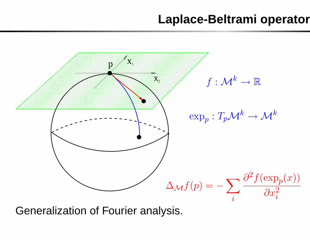
Laplace-Beltrami operator

��

��

2x

1p x

f :Mk→ R

expp : TpMk→M

k

∆Mf(p) = −∑

i

∂2f(expp(x))

∂x2i

Generalization of Fourier analysis.

Algorithmic framework: Laplacian

f

f ff 1

f

f

2

3 4

5

6

L =

2 −1 −1 0 0 0

−1 2 −1 0 0 0

−1 −1 3 −1 0 0

0 0 −1 3 −1 −1

0 0 0 −1 2 −1

0 0 0 −1 −1 2

Natural smoothness functional (analogue of grad):

S(f) = (f1−f2)2+(f1−f3)

2+(f2−f3)2+(f3−f4)2+(f4−f5)2+(f4−f5)

2+(f5−f6)2

Basic fact:

S(f) =∑

i∼j

(fi − fj)2 =

1

2ftL f

Algorithmic framework

Algorithmic framework

Wij = e−‖xi−xj‖

2

t

Lf(xi) = f(xi)∑

j

e−‖xi−xj‖

2

t −

∑

j

f(xj)e−

‖xi−xj‖2

t

ftL f = 2

∑

i∼j

e−‖xi−xj‖

2

t (fi − fj)2

Data representation

f : G→ R

Minimize∑

i∼j wij(fi − fj)2

Preserve adjacency.

Solution: Lf = λf (slightly better Lf = λDf)Lowest eigenfunctions of L (L̃).

Laplacian EigenmapsBelkin Niyogi 01

Related work: LLE: Roweis, Saul 00; Isomap: Tenenbaum, De Silva, Langford 00

Hessian Eigenmaps: Donoho, Grimes, 03; Diffusion Maps: Coifman, et al, 04

Laplacian Eigenmaps

� Visualizing spaces of digits and sounds.Partiview, Ndaona, Surendran 04

� Machine vision: inferring joint angles.Corazza, Andriacchi, Stanford Biomotion Lab, 05, Partiview, Surendran

Isometrically invariant representation. [link]

� Reinforcement Learning: value functionapproximation. Mahadevan, Maggioni, 05

Semi-supervised learning

Learning from labeled and unlabeled data.� Unlabeled data is everywhere. Need to use it.� Natural learning is semi-supervised.

Semi-supervised learning

Learning from labeled and unlabeled data.� Unlabeled data is everywhere. Need to use it.� Natural learning is semi-supervised.

Idea:construct the Laplace operator using unlabeled data.

Fit eigenfunctions using labeled data.

Toy example

−1 0 1 2

−1

0

1

2

γA = 0.03125 γ

I = 0

SVM

−1 0 1 2

−1

0

1

2

Laplacian SVM

γA = 0.03125 γ

I = 0.01

−1 0 1 2

−1

0

1

2

Laplacian SVM

γA = 0.03125 γ

I = 1

Experimental comparisons

Dataset → g50c Coil20 Uspst mac-win WebKB WebKB WebKB

Algorithm ↓ (link) (page) (page+link)

SVM (full labels) 3.82 0.0 3.35 2.32 6.3 6.5 1.0

SVM (l labels) 8.32 24.64 23.18 18.87 25.6 22.2 15.6

Graph-Reg 17.30 6.20 21.30 11.71 22.0 10.7 6.6

TSVM 6.87 26.26 26.46 7.44 14.5 8.6 7.8

Graph-density 8.32 6.43 16.92 10.48 - - -

∇TSVM 5.80 17.56 17.61 5.71 - - -

LDS 5.62 4.86 15.79 5.13 - - -

LapSVM 5.44 3.66 12.67 10.41 18.1 10.5 6.4

Key theoretical question

What is the connection between point-cloud LaplacianL and Laplace-Beltrami operator ∆M?

Analysis of algorithms:

Eigenvectors of L?←→ Eigenfunctions of ∆M

Convegence

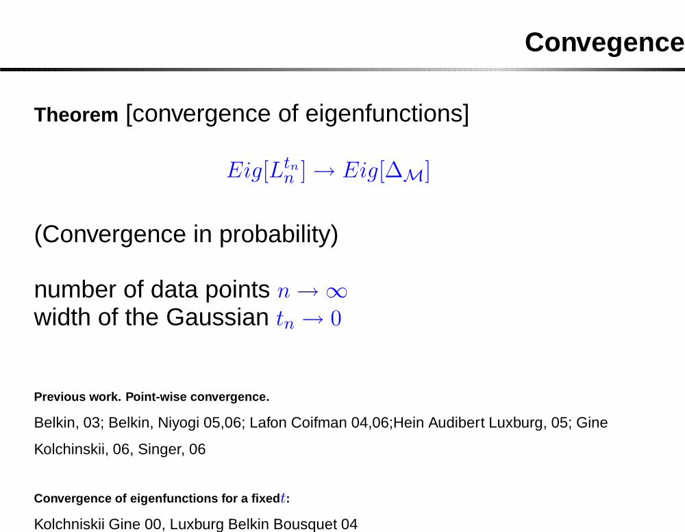
Theorem [convergence of eigenfunctions]

Eig[Ltn

n ]→ Eig[∆M]

(Convergence in probability)

number of data points n→∞

width of the Gaussian tn → 0

Previous work. Point-wise convergence.

Belkin, 03; Belkin, Niyogi 05,06; Lafon Coifman 04,06;Hein Audibert Luxburg, 05; Gine

Kolchinskii, 06, Singer, 06

Convergence of eigenfunctions for a fixed t:

Kolchniskii Gine 00, Luxburg Belkin Bousquet 04

Recall

Heat equation in Rn:

u(x, t) – heat distribution at time t.u(x, 0) = f(x) – initial distribution. x ∈ R

n, t ∈ R.

∆Rnu(x, t) =du

dt(x, t)

Solution – convolution with the heat kernel:

u(x, t) = (4πt)−n

2

∫

Rn

f(y)e−‖x−y‖2

4t dy

Proof idea (pointwise convergence)

Functional approximation:Taking limit as t→ 0 and writing the derivative:

∆Rnf(x) =d

dt

[

(4πt)−n

2

∫

Rn


4t dy

]

0



∆Rnf(x) =d

dt

[

(4πt)−n

2

∫

Rn


4t dy

]

0

∆Rnf(x) ≈ −1

t(4πt)−

n

2

(

f(x)−

∫

Rn


4t dy

)



∆Rnf(x) =d

dt

[

(4πt)−n

2

∫

Rn


4t dy

]

0

∆Rnf(x) ≈ −1

t(4πt)−

n

2

(

f(x)−

∫

Rn


4t dy

)

Empirical approximation:Integral can be estimated from empirical data.

∆Rnf(x) ≈ −1

t(4πt)−

n

2

(

f(x)−∑

xi

f(xi)e−

‖x−xi‖2

4t

)

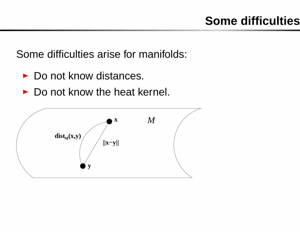
Some difficulties

Some difficulties arise for manifolds:

� Do not know distances.� Do not know the heat kernel.

||x−y||

x

y

M

dist (x,y)M

Some difficulties

Some difficulties arise for manifolds:

� Do not know distances.� Do not know the heat kernel.

||x−y||

x

y

M

dist (x,y)M

Careful analysis required.

Mesh Laplacian

Mesh Laplacian

Mesh K.

Triangle t. Area A(t).

Vertices v, w.

LKf(w) =1

4πt2

∑

t∈K

A(t)

3

∑

v∈t

e−‖p−w‖2

4t (f(v)− f(

Belkin Sun Wang, 07

Convergence

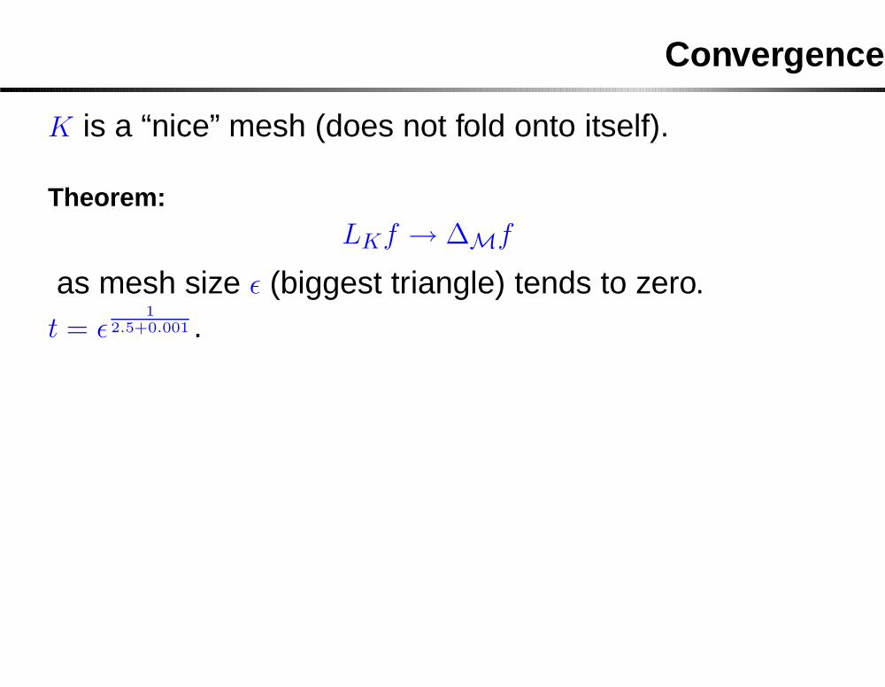
K is a “nice” mesh (does not fold onto itself).

Theorem:LKf → ∆Mf

as mesh size ε (biggest triangle) tends to zero.t = ε

1

2.5+0.001 .

Convergence

K is a “nice” mesh (does not fold onto itself).

Theorem:LKf → ∆Mf

as mesh size ε (biggest triangle) tends to zero.t = ε

1

2.5+0.001 .

500 pts 2000 pts 8000 pts

Eig #1 0.004 0.003 0.0009

Eig #7 0.020 0.008 0.007

Eig #50 0.112 0.029 0.010

Mesh Laplacian

Existing work: several methods, includingDesbrun, et al 99, Meyer, et al 02, Xu 04. Numerousapplications (smoothing, quadrangulations, deformations, etc).

Mesh Laplacian

Existing work: several methods, includingDesbrun, et al 99, Meyer, et al 02, Xu 04. Numerousapplications (smoothing, quadrangulations, deformations, etc).None converge even in R

2.

Mesh Laplacian

Existing work: several methods, includingDesbrun, et al 99, Meyer, et al 02, Xu 04. Numerousapplications (smoothing, quadrangulations, deformations, etc).None converge even in R

2.

f = x2 500 pts 2000 pts 8000 pts

Meyer 0.481 0.256 0.357

Xu 0.220 0.173 0.197

MLap 0.069 0.017 0.004

Conclusions

� Laplacian carries extensive geometric information.

Conclusions

� Laplacian carries extensive geometric information.� Theoretically grounded and practical methods.

Conclusions


(Yes, it is possible!)

Conclusions


(Yes, it is possible!)� Interesting connections between machine learning

and graphics.

Conclusions


(Yes, it is possible!)� Interesting connections between machine learning

and graphics.� More things should be possible now.

constructing laplace operators from data - …saito/lapeig/belkin.pdfconstructing laplace operators...

Documents