constructing uncertainty sets for robust linear...
TRANSCRIPT
Constructing uncertainty sets for robust linear optimization
Dimitris Bertsimas∗ David B. Brown†
July 17, 2007
Abstract
In this paper, we propose a methodology for constructing uncertainty sets within the framework
of robust optimization for linear optimization problems with uncertain parameters. Our approach
relies on decision-maker risk preferences. Specifically, we utilize the theory of coherent risk measures
initiated by Artzner et al. [3], and show that such risk measures, in conjunction with the support of
the uncertain parameters, are equivalent to explicit uncertainty sets for robust optimization. We also
explore the structure of these sets. In particular, we study a class of coherent risk measures, called
spectral risk measures, which give rise to polyhedral uncertainty sets of a very specific structure which
is tractable in the context of robust optimization. In the case of discrete distributions with rational
probabilities, which is useful in practical settings when we are sampling from data, we show that the
class of all spectral risk measures (and their corresponding polyhedral sets) are finitely generated. A
subclass of the spectral measures corresponds to polyhedral uncertainty sets symmetric through the
sample mean. We show that this subclass is also finitely generated and can be used to find inner
approximations to arbitrary, polyhedral uncertainty sets.
Keywords: robust optimization, uncertainty sets, coherent risk measures, spectral risk measures.
∗Boeing Professor of Operations Research, Sloan School of Management and Operations Research Center, Massachusetts
Institute of Technology, E40-147, Cambridge, MA 02139, [email protected].†Assistant Professor of Decision Sciences, The Fuqua School of Business, Duke University, 1 Towerview Drive, Durham,
NC 27708, [email protected].
1

1 Introduction
Robust optimization dates back at least 30 years to the work of Soyster [30]. With the advent of efficient
algorithms for conic optimization problems, the field of robust optimization has expanded significantly
over the past decade. Helping to spark this recent growth was the work of Ben-Tal and Nemirovski
[4, 5], who show that even small perturbations of uncertain quantities can result in highly infeasible
solutions. More recent work has focused on the properties of the solutions and the tractability of various
robust formulations, as well extending robustness to more general conic problems (e.g., Bertsimas et al.
[7], Bertsimas and Sim [8], El Ghaoui and Lebret [15], and El Ghaoui et al. [15]).
In this paper, we consider the case of robust optimization in the context of linear optimization
problems. In particular, for linear optimization with uncertain constraint matrix A, the robust problem
is without loss of generality in the form:
minc′x : Ax ≤ b ∀ A ∈ U.
where x ∈ Rn is a decision vector, c ∈ Rn, b ∈ Rm, A ∈ Rm×n is a matrix of uncertain coefficients,
and U is an uncertainty set for A. Note that this form is general enough to capture uncertainty in the
right-hand side vector and the cost vector as well; indeed, if b is uncertain, we may add a variable xn+1
and include b as a column of the matrix A and constrain xn+1 = 1, and, if c is uncertain, we may add
a variable t and the constraint c′x ≥ t, and change the objective to minimizing t.
The idea of the robust optimization approach is to compute optimal solutions which retain fea-
sibility for all possible realizations of A within this prescribed uncertainty set U . The literature on
robust optimization, however, is essentially silent on the the question of constructing these uncertainty
sets. Ellipsoidal uncertainty sets, as well as other norms are common in many treatments (e.g., [7]).
Although often rooted in some statistical considerations, these approaches are fundamentally ad hoc,
with emphasis usually placed on sets that preserve computational tractability.
Here we provide a prescriptive methodology for constructing uncertainty sets within a robust op-
timization framework for linear optimization problems with uncertain data. We accomplish this by
taking as primitive the decision-maker’s attitude towards risk. We show that when this attitude can be
expressed in the form of a coherent risk measure (Artzner et al., [3]), then the optimization problem with
this risk aversion is equivalent to a robust optimization problem with an explicit, convex uncertainty
set.
Our approach is “data-driven,” i.e., the only information on the uncertain matrix A at our disposal
is a finite set of sampled matrices A1, . . . , AN . In addition to avoiding complicated, distributional
assumptions, this data-driven approach is well-suited to practical settings, in which the realizations of
the uncertain parameters are typically the only information available.
We summarize our key results as follows:
2

1. Given a coherent risk measure as a primitive, as well as realizations of the uncertain data in the
problem, we construct a corresponding convex uncertainty set in a robust optimization framework.
This is important as the uncertainty set becomes a consequence of the particular risk measure the
decision maker selects. Thus, risk preferences which can be expressed in the form of a coherent
risk measure lead to convex uncertainty sets of an explicit construction. A converse implication
naturally holds; uncertainty sets within the parameter support induce a coherent risk measure.
2. We consider an important subclass of coherent risk measures, called spectral risk measures (nomen-
clature introduced by Acerbi [1]), which satisfy some additional risk hedging and distribution
invariance properties. In the case of a discrete distribution over rational probabilities (which
may always be converted to a uniform one over a potentially larger probability space), we show
that these spectral measures are finitely generated by a finite number of conditional value-at-
risk (CVaR) measures. Furthermore, we show that spectral measures correspond to uncertainty
polytopes with a special structure that allows for efficiently solvable robust linear programs.
3. A further subclass of spectral risk measures induce uncertainty polytopes which are symmetric
through the sample mean regardless of the underlying support. We show that this subclass is also
finitely generated. Moreover, these symmetric uncertainty sets may be described by a norm and
can be used to find inner approximations to arbitrary polyhedral sets, as we show.
We emphasize that we are attempting to make a contribution to robust optimization, not risk theory.
For the most part, we are leveraging known results from risk theory to develop our approach. Indeed,
the risk theory community is generally focused on more general probability spaces; as we have stated,
our restriction to discrete spaces is motivated in part by the practical issue of sampling, as well as
ease of insight into the geometry of the resulting uncertainty sets (e.g., associating extreme points with
mixtures of particular “outlier” samples, etc.).1
A contemporaneous paper done independently by Natarajan et al. [24] also explores the connection
between risk measures and uncertainty sets. The thrust of their work, however, is to derive risk measures
from uncertainty sets. The focus of our work here, on the other hand, is on a methodology for uncertainty
set construction beginning with a risk measure as a primitive. Recent work by Chen et al. [10] also
considers using the CVaR risk measure as a tractable means of constructing uncertainty sets in the
context of optimization problems with multiple chance constraints.
The outline of the paper is as follows. Section 2 introduces some necessary background from risk
theory. Section 3 considers general coherent risk measures. Section 4 introduces spectral risk measures
and develops the associated polyhedral uncertainty sets in detail. Section 5 concludes the paper.1For some more recent work using samples in the context of chance-constrainted optimization, see, e.g., Calafiore and
Campi [9] and Nemirovski and Shapiro [26].
3

Notation: Throughout the paper, e will denote the vector of ones and eN , e/N . We will denote
the N -dimensional probability simplex by ∆N , i.e.,
∆N =p ∈ RN
+ : e′p = 1
.
2 Background from risk theory
Before describing our approach to constructing uncertainty sets, we need some background from risk
theory.
2.1 Risk measures
Consider a probability space (Ω,F ,P). Let X be a linear space of random variables on Ω, i.e., a set of
functions X : Ω → R. It is typically assumed that X ⊆ L∞(Ω,F ,P).2 X, for the introduction, can be
thought of as a reward from an uncertain position. We will use the notation X ≥ Y for X, Y ∈ X to
represent state-wise dominance, i.e., X(ω) ≥ Y (ω) for all ω ∈ Ω.
We have the following definition.
Definition 2.1. A function µ : X → R which satisfies, for all X, Y ∈ X :
1. Monotonicity : If X ≥ Y , then µ(X) ≤ µ(Y );
2. Translation invariance: If c ∈ R, then µ(X + c) = µ(X)− c,
is called a risk measure.
A risk measure can be interpreted as the smallest amount of capital necessary to by which to augment
a position X in order to make it “acceptable” according to some standard. As such, the properties above
are clear; if one position X never performs worse than another position Y , then it cannot be any riskier.
In addition, if we augment our position by a guaranteed amount c, then our capital requirement is
reduced correspondingly by c as well. A classic example of a risk measure is the so-called value-at-risk
defined as
VaRα (X) , inf t ∈ R : P [t + X ≥ 0] ≥ 1− α .
This risk measure can be interpreted as the smallest amount of additional capital required to ensure
that a position breaks even with probability at least 1− α. See, for instance, Follmer and Schied [19]
for more on risk measures.2Obviously, when we impose that |Ω| must be finite and supported by finite elements, such boundedness concerns
disappear.
4
2.2 Coherent risk measures
Although a risk measure need only satisfy translation invariance and monotonicity, we may desire
additional, structural properties, such as the way risk measures should deal with diversification, etc.
Artzner et al. [3] present an axiomatic definition of risk measures satisfying some natural properties
and termed such measures coherent, as we now define.
Definition 2.2. A function µ : X → R which, in addition to being a risk measure, satisfies, for all
X, Y ∈ X :
1. Convexity : If λ ∈ [0, 1], then µ(λX + (1− λ)Y ) ≤ λµ(X) + (1− λ)µ(Y );
2. Positive homogeneity : If λ ≥ 0, then µ(λX) = λµ(X),
is called a coherent risk measure.
The intuition behind these axioms is fairly clear. For instance, the convexity property ensures that
diversification of positions can never increase risk under a coherent risk measure; this is desirable for
both economic reasons (convex preferences) and computational ones (ensuring that optimization over
risk measures induces convex optimization problems). The positive homogeneity axiom states that risk
scales linearly with the size of a position; when this axiom is lifted, we obtain the more general class of
convex risk measures introduced by Follmer in Schied [18]. Note also that, when positive homogeneity
holds, the convexity axiom is equivalent to the requirement of subadditivity, i.e., µ(X+Y ) ≤ µ(X)+µ(Y )
for all X, Y ∈ X .
One of most noteworthy coherent risk measures is the conditional value-at-risk, defined as
µ(X) , infν∈R
ν +
1αE
[(−ν −X)+
].
This coherent risk measure explored in detail by Rockafellar and Uryasev [28]. For atomless distribu-
tions, this is equivalent to −E [X | X ≤ −VaRα (X)]. Delbaen [12] shows that CVaR is the smallest
upper bound to VaR among all coherent risk measures which depend only on the distribution of the
underlying random variable. Acerbi and Tasche [2] define the same risk measure but name it expected
shortfall (explored also by Bertsimas et al., [6]). Nemirovski and Shapiro [25] use CVaR as a means of
finding convex approximations to chance constrained optimization problems.
We will also find this risk measure to be of central importance and it will have a variety of interesting
properties which we will examine and discuss in Section 4.
2.3 Representation theorem for coherent risk measures
The following is the main result related to coherent risk measures. In essence it states that we can
describe any coherent risk measure equivalently in terms of expectations over a family of distributions.
5
The result is largely a consequence the separation theorem for convex sets. The proof actually predates
the introduction of coherent risk measures (see, e.g., chapter 10 of Huber [20] for one version of the
proof).
Theorem 2.1. [Representation of coherent risk measures]: A function µ : X → R is a coherent risk
measure if and only if there exists a family of probability measures Q on (Ω,F) with Q ¿ P for all
Q ∈ Q such that
µ(X) = supQ∈Q
EQ [−X] , ∀ X ∈ X , (1)
where EQ [X] denotes the expectation of the random variable X under the measure Q (as opposed to the
measure of X itself).3
The representation theorem says that all coherent risk measures may be represented as the worst-
case expected value over a family of “generalized scenarios.” For example, the generating family for
CVaR is Q = Q¿ P : Q ≤ P/α.This is a duality theorem and the connection to robustness is clear; a risk measure is coherent if
and only if it can be expressed as the worst-case expected value over a family of distributions. This is a
very clear ambiguity interpretation and is the crucial idea as we attempt to construct uncertainty sets
in a robust optimization framework from a given coherent risk measure.
3 Coherent risk measures and convex uncertainty
In this section, we show how the concepts from risk theory, in particular, coherent risk measures, allow
us to construct a robust counterpart to a linear optimization problem with uncertain data. We will
focus on a single constraint of the form a′x ≥ b. For multiple constraints, we can obviously apply this
framework in constraint-wise fashion; on the other hand, depending on how we wish to weigh the risk
associated with the various constraints, this may or may not be appropriate. The issue of vector-valued
risk measures is an interesting one and very much open; see, for instance, Jouini et al. [21] for an effort
at extending coherent risk measures to more general vector spaces. Our focus, therefore, is on a single
constraint.
We note the following issues in a practical context.
(1) We generally do not know the distribution of a. In fact, we usually only have some finite number
N of observations of the uncertain vector a.
(2) Even equipped with a perfect description of the distribution of a, it is not clear how we should
construct an uncertainty set U within a robust optimization setting.3This is the general result; again, in the case of discrete probability spaces with nonzero probabilities, absolute continuity
conditions are automatically ensured and need not be stated explicitly.
6

To address the first issue, we will make the following assumption.
Assumption 3.1. The uncertain vector a is a random variable in Rn on the finite probability space
(Ω,F ,P) where |Ω| = N , F = 2Ω. We denote ai , a(ωi) and the support of a by A = a1, . . . ,aN.
Remark 3.1. Actually, this assumption is not really needed for the results in this section; the result will
still go through for infinite probability spaces (see [24]). As our underlying motivation in this paper
is the case in which we are data-driven, and because we will rely heavily on the discrete space in the
following sections, however, we adopt the assumption now.
Remark 3.2. We will occasionally refer to A as the data of the problem. In some cases, it will also be
convenient to use the matrix form A = [a1 · · ·aN ].
Thus, we assume that the sample space is confined to a1, . . . ,aN, and a is distributed across these
N values. Although this may seem restrictive, it is in practice quite useful as the data are many times
the only information we have about the distribution of a.
For the second issue, we take as primitive a coherent risk measure. The choice of this risk measure
clearly depends on the preferences of the decision-maker. Given a constraint based on this coherent
risk measure and distribution defined as above, we will show that there exists an equivalent robust
optimization problem with a unique convex uncertainty set.
Specifically, the decision-maker would like to ensure some level of conservatism for satisfying the
constraint and they impose this with a risk aversion constraint of the form µ(a′x − b) ≤ 0. This is
appropriate in situations when simply taking the expected value of a is not a good enough guarantee;
notice also that this constraint is convex in x, which contrasts with the approach of chance constraints
often proposed as a method for embedding conservatism into the optimization problem.
To put this into more concrete terms, imagine x to be an decision vector representing allocation
across n production units with uncertain production levels a; we are concerned about the possibility
of not meeting a particular total production level b. Meeting b in expectation is simply not a good
enough guarantee. Of course, we could enforce P [a′x ≥ b] ≥ 1 − α for some sufficiently small α, but
this destroys convexity of the problem in general.
A coherent risk measure, on the other hand, is an approach which allows us to obtain some de-
gree of conservatism without compromising convexity of the problem. For instance, the constraint
CVaRα (a′x− b) ≤ 0 says, roughly,4 that the expected value of the total production, in the α% worst
cases, is no less than b. Notice also that this implies P [a′x ≥ b] ≥ 1− α.
We have the first result, which stems in straightforward fashion from Theorem 2.1.
Theorem 3.1. If the risk measure µ is coherent and a is distributed as in Assumption 3.1, then
x ∈ Rn : µ(a′x− b) ≥ 0
=
x ∈ Rn : a′x ≥ b ∀ a ∈ U
, (2)
4Again, this interpretation is not exact if the distribution is not atomless, but it is approximately true. We are just
trying to provide intuition here.
7
where
U = conv (Aq : q ∈ Q),
and Q is the family of generating measures for µ. Conversely, if U ⊆ conv (A), then (2) holds with the
coherent risk measure generated by
Q =q ∈ ∆N : ∃ a ∈ U s.t. Aq = a
.
Proof. Assume µ is given and coherent; by Theorem 2.1 and the fact that a is distributed on A, we
have
µ(a′x− b) = µ(a′x) + b
= supQ∈Q
EQ
[−a′x]+ b
= supq∈Q
−(Aq)′x
+ b
= − infa∈U
a′x
+ b
= − infa∈U
a′x
+ b
where U = Aq : q ∈ Q and U = conv(U) and the last line follows from the simple observation that
the inf of a linear function over any bounded set is equal to the inf of that function over the convex hull
of that set. The converse direction follows in nearly identical fashion with the steps reversed.
Theorem 3.1 provides a methodology for constructing robust optimization problems with uncertainty
sets possessing a direct, physical meaning. The decision-maker has some risk measure µ which depends
on their preferences. If µ is coherent, there is an explicit uncertainty set that should be used in the robust
optimization framework. This uncertainty set is convex and its structure depends on the generating
family Q for µ and the data A. We provide a few examples.
Example 3.1. Scenario-based sets: Consider the coherent risk measure generated by
Q = conv (q1, . . . , qm) ,
where qi ∈ ∆N . This is simply a coherent risk measure based on scenarios for the underlying distribution
and the connection to robustness is transparent. The uncertainty set is just
U = conv (Aq1, . . . , Aqm) .
Example 3.2. Conditional value-at-risk : For CVaR, we have the generating family Q = q ∈ ∆N :
qi ≤ pi/α. This leads to the uncertainty set
U = conv
(1α
∑
i∈I
piai +
(1− 1
α
∑
i∈I
pi
)aj : I ⊆ 1, . . . , N, j ∈ 1, . . . , N \ I,
∑
i∈I
pi ≤ α
).
8
This set is a polytope. When pi = 1/N and α = j/N for some j ∈ Z+, this has the interpretation of
the convex hull of all j-point averages of A. We will explore these kinds of sets in much more detail in
the following section.
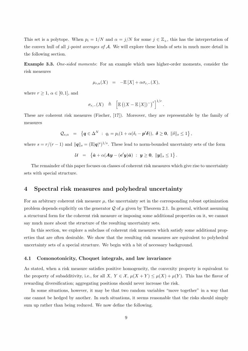
Example 3.3. One-sided moments: For an example which uses higher-order moments, consider the
risk measures
µr,α(X) = −E [X] + ασr,−(X),
where r ≥ 1, α ∈ [0, 1], and
σr,−(X) ,[E
((X − E [X])−
)r]1/r
.
These are coherent risk measures (Fischer, [17]). Moreover, they are representable by the family of
measures
Qs,α =q ∈ ∆N : qi = pi(1 + α(δi − p′δ)), δ ≥ 0, ‖δ‖s ≤ 1
,
where s = r/(r − 1) and ‖q‖s = (E|q|s)1/s. These lead to norm-bounded uncertainty sets of the form
U =a + α(Ay − (e′y)a) : y ≥ 0, ‖y‖s ≤ 1
.
The remainder of this paper focuses on classes of coherent risk measures which give rise to uncertainty
sets with special structure.
4 Spectral risk measures and polyhedral uncertainty
For an arbitrary coherent risk measure µ, the uncertainty set in the corresponding robust optimization
problem depends explicitly on the generator Q of µ given by Theorem 2.1. In general, without assuming
a structural form for the coherent risk measure or imposing some additional properties on it, we cannot
say much more about the structure of the resulting uncertainty sets.
In this section, we explore a subclass of coherent risk measures which satisfy some additional prop-
erties that are often desirable. We show that the resulting risk measures are equivalent to polyhedral
uncertainty sets of a special structure. We begin with a bit of necessary background.
4.1 Comonotonicity, Choquet integrals, and law invariance
As stated, when a risk measure satisfies positive homogeneity, the convexity property is equivalent to
the property of subadditivity, i.e., for all X, Y ∈ X , µ(X + Y ) ≤ µ(X) + µ(Y ). This has the flavor of
rewarding diversification; aggregating positions should never increase the risk.
In some situations, however, it may be that two random variables “move together” in a way that
one cannot be hedged by another. In such situations, it seems reasonable that the risks should simply
sum up rather than being reduced. We now define the following.
9

Definition 4.1. Two random variables X, Y ∈ X which satisfy, for all (ω, ω′) ∈ Ω2,
(X(ω)−X(ω′))(Y (ω)− Y (ω′)) ≥ 0
are called comonotone. A risk measure µ : X → R which satisfies, for all comonotone X, Y ∈ X
µ(X + Y ) = µ(X) + µ(Y ),
is called comonotonic.
As a simple example, consider a call option with strike price K and the price S of the underlying
stock. The exercise value is C = max(0, S − K). Clearly S and C are comonotone. In this case, a
comonotonic risk measure would not allow us to reduce the risk of a position in the stock with a position
in the call.
On a related note, comonotonicity is an important property when considering sums of random vari-
ables with arbitrary dependencies. Comonotone random variables have worst-case summation properties
among all dependence structures, and, as such, have been used by Dhaene et al. [14] to compute upper
bounds on sums of random variables. Coherent risk measures that are also comonotonic are linked to
Choquet integrals, which we now define with some more terminology.
Definition 4.2. A set function g : F → [0, 1] is called monotone if g(A) ≤ g(B) for all A ⊆ B ⊆ Ω and
normalized if g(∅) = 0 and g(Ω) = 1. If, in addition, g satisfies
g(A ∪B) + g(A ∩B) ≤ g(A) + g(B),
we say g is submodular.
This now allows us to define the Choquet integral, introduced in [11].
Definition 4.3. The Choquet integral of a random variable X ∈ X with respect to the monotone,
normalized set function g : F → [0, 1] is defined as
∫Xdg ,
0∫
−∞(g(X > x)− 1)dx +
∞∫
0
g(X > x)dx. (3)
Choquet integrals have been used in the application of pricing insurance premia (e.g., Denneberg
[13], Wang [31]). The following result is due to Schmeidler [29].
Theorem 4.1. [Schmeidler] A coherent risk measure µ : X → R is comonotonic if and only if it can
be written in the form∫
(−X)dg where g : F → [0, 1] is a monotone, normalized, and submodular set
function.
10

For example, CVaR can be written as the Choquet integral of the function g(A) = minP [A] /α, 1,which is clearly monotone, normalized, and submodular; this alone tells us that CVaR is comonotonic
and coherent.
We define one more property of risk measures; this property is intimately connected to their esti-
mation from historical data.
Definition 4.4. A risk measure µ : X → R which satisfies µ(X) = µ(Y ) for all X, Y ∈ X such that X
and Y have the same distribution under P is called law-invariant.
Law-invariance is a very sensible property when we are dealing with the situation when we are
estimating risk measures from data, which is our motivation. In fact, if a risk measure is not law-
invariant, then we are generally not able to estimate it from data. Indeed, consider X and Y with
the same distribution and let µ be a risk measure such that µ(X) 6= µ(Y ). Let Xi and Yi be a
sequence of N IID samples of X and Y . As N → ∞, the sequences are asymptotically identical, so
limN→∞ µ(Xi) = limN→∞ µ(Yi). Therefore, the estimator must not converge to the true value in
general.
Summarizing the properties in this section, we introduce the following name, due to Acerbi [1].
Definition 4.5. A coherent risk measure which is also comonotonic and law-invariant is called spectral.
4.2 Representation of spectral risk measures
We now show a representation theorem for spectral risk measures. Throughout the remainder of the
paper, we will operate under the following assumption.
Assumption 4.1. The distribution P satisfies P [ωi] = 1/N for all i ∈ 1, . . . , N.
Remark 4.1. Although this is obviously a very special distribution, it is not a very limiting assumption
given that we have already restricted ourselves to discrete spaces. One of the central motivations of
this paper is to explore the connection between risk measures and uncertainty sets in the setting, very
common in practice, in which we are obtaining distributional information from samples. As such, this
is obviously far and away the most relevant discrete distribution; of course, it also encompasses any
distribution P [ωi] = ki/N where ki ∈ Z+ and k1 ∪ · · · ∪ kN is any partition of N as well, simply by
replicating samples (or discarding them if ki = 0). Furthermore, given an arbitrary, discrete distribution
representable with rational numbers, we may always convert it to such a form for some N . The price
we will pay for such a conversion to a larger N will be a complexity one in terms of the size of the
corresponding robust problem; we will see this explicitly in the next section.
We now work towards a representation theorem, which tells us that a risk measure in this setting is
spectral if and only if it is a mixture of CVaR measures. We start with the following lemma.
11
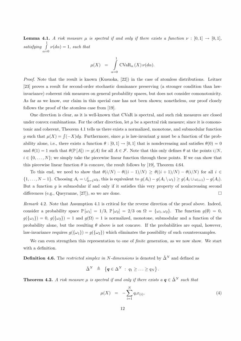
Lemma 4.1. A risk measure µ is spectral if and only if there exists a function ν : [0, 1] → [0, 1],
satisfying1∫
α=0
ν(dα) = 1, such that
µ(X) =
1∫
α=0
CVaRα (X) ν(dα).
Proof. Note that the result is known (Kusuoka, [22]) in the case of atomless distributions. Leitner
[23] proves a result for second-order stochastic dominance preserving (a stronger condition than law-
invariance) coherent risk measures on general probability spaces, but does not consider comonotonicity.
As far as we know, our claim in this special case has not been shown; nonetheless, our proof closely
follows the proof of the atomless case from [19].
One direction is clear, as it is well-known that CVaR is spectral, and such risk measures are closed
under convex combinations. For the other direction, let µ be a spectral risk measure; since it is comono-
tonic and coherent, Theorem 4.1 tells us there exists a normalized, monotone, and submodular function
g such that µ(X) =∫
(−X)dg. Furthermore, since µ is law-invariant g must be a function of the prob-
ability alone, i.e., there exists a function θ : [0, 1] → [0, 1] that is nondecreasing and satisfies θ(0) = 0
and θ(1) = 1 such that θ(P [A]) := g(A) for all A ∈ F . Note that this only defines θ at the points i/N ,
i ∈ 0, . . . , N; we simply take the piecewise linear function through these points. If we can show that
this piecewise linear function θ is concave, the result follows by [19], Theorem 4.64.
To this end, we need to show that θ(i/N) − θ((i − 1)/N) ≥ θ((i + 1)/N) − θ(i/N) for all i ∈1, . . . , N − 1. Choosing Ai = ∪i
k=1ωk, this is equivalent to g(Ai)− g(Ai \ ω1) ≥ g(Ai ∪ ωi+1)− g(Ai).
But a function g is submodular if and only if it satisfies this very property of nonincreasing second
differences (e.g., Queyranne, [27]), so we are done.
Remark 4.2. Note that Assumption 4.1 is critical for the reverse direction of the proof above. Indeed,
consider a probability space P [ω1] = 1/3, P [ω2] = 2/3 on Ω = ω1, ω2. The function g(∅) = 0,
g(ω1) = 0, g(ω2) = 1 and g(Ω) = 1 is normalized, monotone, submodular and a function of the
probability alone, but the resulting θ above is not concave. If the probabilities are equal, however,
law-invariance requires g(ω1) = g(ω2) which eliminates the possibility of such counterexamples.
We can even strengthen this representation to one of finite generation, as we now show. We start
with a definition.
Definition 4.6. The restricted simplex in N -dimensions is denoted by ∆N and defined as
∆N ,q ∈ ∆N : q1 ≥ . . . ≥ qN
.
Theorem 4.2. A risk measure µ is spectral if and only if there exists a q ∈ ∆N such that
µ(X) = −N∑
i=1
qix(i), (4)
12

where x(i) are the increasing order statistics of X, i.e., x(1) ≤ . . . ≤ x(N). Moreover, every such q ∈ ∆N
may be written in the form
q =N∑
i=1
λj qj , (5)
where λ ≥ 0,N∑
j=1λj = 1 and qj ∈ ∆N corresponds to the spectral risk measure CVaRj/N .
Proof. First, consider a risk measure given as in (4). Such a risk measure is coherent, as it is generated
by the set Q = q′ ∈ ∆N : q′i = qσ(i), σ ∈ S(N), where S(N) is all permutations of N elements. It
also obviously comonotone. Law-invariance follows, since, if X and Y have the same distribution under
Assumption 4.1, they must have x(i) = y(i) for all i ∈ 1, . . . , N (this would not be true on an arbitrary
discrete distribution).
For the other direction of the first part, note that we have, for α ≥ 1/N ,
CVaRα (X) = supq∆N : qi≤1/(Nα)
Eq [−X]
= − 1Nα
bNαc∑
i=1
x(i) −(
Nα− bNαcbNαc
)x(dNαe)
, −N∑
i=1
qαi x(i),
(and for α < 1/N we have qα = q1/N ). Via Lemma 4.1, we can write µ in the form (4) with qi =∫qαi ν(dα); since qα ∈ ∆N , we have q ∈ ∆N as well, which completes the first part of the proof.
To show finite generation of q, consider the matrix QN with columns qj , i.e.,
QN =
1 · · · 1N−2
1N−1
1N
......
......
...
0 0 1N−2
1N−1
1N
0 · · · 0 1N−1
1N
0 · · · 0 0 1N
,
and define the vector λ ∈ RN as λN = NqN , λN−j = (N−j)(qN−j−qN−j+1), for all j ∈ 1, . . . , N−1.We have q ∈ ∆N , so qj ≤ qj+1 and thus λ ≥ 0. In addition,
N∑
j=1
λj =N∑
j=1
qj = 1.
Finally, we compute the vector QNλ and see that
[QNλ]i =i∑
j=1
1N − j + 1
λN−j+1
= qN + (qN−1 − qN ) + · · ·+ (qi+1 − qi+2) + (qi − qi+1)
= qi,
13

πq(A), q = (1/5, 1/5, 1/5, 1/5, 1/5) a5
a2
a1
πq(A), q = (0, 0, 0, 0, 1)
πq(A), q = (0, 0, 0, 1/2, 1/2)
πq(A), q = (0, 1/4, 1/4, 1/4, 1/4)
a4
a3
Figure 1: Πq (A) for various q for an example with N = 5.
which completes the proof.
4.3 Connecting to polyhedral uncertainty
With the representation for spectral measures in hand, we now connect to their induced uncertainty
sets. Theorem 4.2 indicates that any spectral risk measure is generated by the family
Q = q′ ∈ ∆N : q′i = qσ(i), σ ∈ S(N)
for some q ∈ ∆N . This motivates the following definition.
Definition 4.7. For some measure q ∈ ∆N and discrete set A = a1, . . . ,aN with ai ∈ Rn for all
i ∈ 1, . . . , N, we define the q-permutohull of A by
Πq (A) = conv
(N∑
i=1
qσ(i)ai : σ ∈ SN
).
Figure 1 illustrates a family of such polyhedra. With most of the work done, we are now able to
link these sets to spectral measures.
Theorem 4.3. If a risk measure µ is spectral, the following hold:
x ∈ Rn : µ(a′x− b) ≥ 0
=x ∈ Rn : a′x ≥ b ∀ a ∈ Πq (A)
=x ∈ Rn : ∃ (y1, y2) ∈ RN × RN , s.t. e′y1 + e′y2 ≥ b, y1,i + y2,j ≤ qi · (a′jx) ∀ (i, j) ∈ 1, . . . , N2
.
Proof. The first equality follows by applying Theorems 3.1 and 4.2. To show the second one, we consider
14
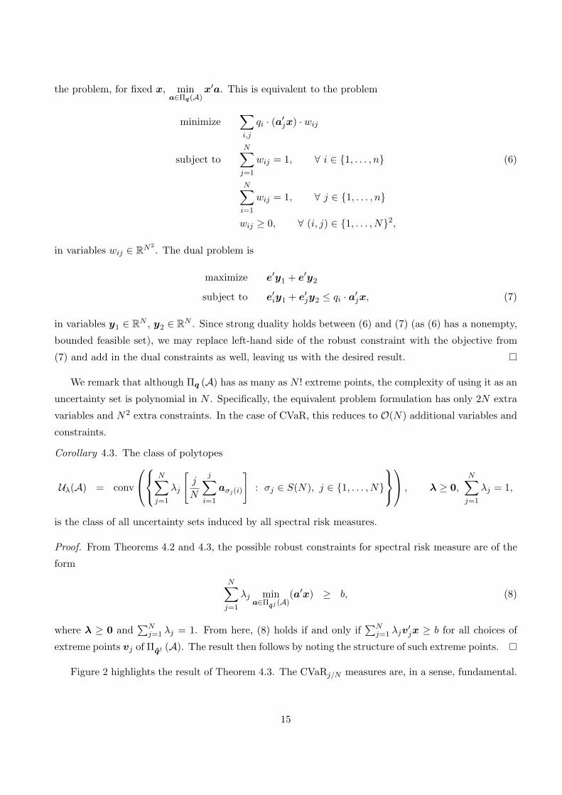
the problem, for fixed x, mina∈Πq(A)
x′a. This is equivalent to the problem
minimize∑
i,j
qi · (a′jx) · wij
subject toN∑
j=1
wij = 1, ∀ i ∈ 1, . . . , n (6)
N∑
i=1
wij = 1, ∀ j ∈ 1, . . . , n
wij ≥ 0, ∀ (i, j) ∈ 1, . . . , N2,
in variables wij ∈ RN2. The dual problem is
maximize e′y1 + e′y2
subject to e′iy1 + e′jy2 ≤ qi · a′jx, (7)
in variables y1 ∈ RN , y2 ∈ RN . Since strong duality holds between (6) and (7) (as (6) has a nonempty,
bounded feasible set), we may replace left-hand side of the robust constraint with the objective from
(7) and add in the dual constraints as well, leaving us with the desired result.
We remark that although Πq (A) has as many as N ! extreme points, the complexity of using it as an
uncertainty set is polynomial in N . Specifically, the equivalent problem formulation has only 2N extra
variables and N2 extra constraints. In the case of CVaR, this reduces to O(N) additional variables and
constraints.
Corollary 4.3. The class of polytopes
Uλ(A) = conv
N∑
j=1
λj
[j
N
j∑
i=1
aσj(i)
]: σj ∈ S(N), j ∈ 1, . . . , N
, λ ≥ 0,
N∑
j=1
λj = 1,
is the class of all uncertainty sets induced by all spectral risk measures.
Proof. From Theorems 4.2 and 4.3, the possible robust constraints for spectral risk measure are of the
form
N∑
j=1
λj mina∈Π
qj (A)(a′x) ≥ b, (8)
where λ ≥ 0 and∑N
j=1 λj = 1. From here, (8) holds if and only if∑N
j=1 λjv′jx ≥ b for all choices of
extreme points vj of Πqj (A). The result then follows by noting the structure of such extreme points.
Figure 2 highlights the result of Theorem 4.3. The CVaRj/N measures are, in a sense, fundamental.
15

q2
q3
N = 3
∆3
N = 4
∆4
q1
q2
q3
q4
(1/2, 1/2)
(0, 0, 1)
(0, 1/2, 1/2)
(0, 0, 0, 1)
(1/3, 1/3, 1/3)
(0, 0, 1/2, 1/2)
(0, 1)
(0, 1/3, 1/3, 1/3)
(1/4, 1/4, 1/4, 1/4)
q2
q1
∆2
N = 2
q1
Figure 2: Generation of ∆N by the CVaR measures for N = 2, 3, 4.
4.4 Spectral risk measures and centrally symmetric polytopes
In this section, we study a more restricted class of generating measures q; specifically, we study those
that lead to polyhedral uncertainty sets obeying a specific symmetry property. These structures are
useful because they naturally induce norm spaces which we will use in the next section to approximate
arbitrary polyhedral uncertainty sets by those corresponding to spectral risk measures.
Definition 4.8. A set P is centrally symmetric through x0 ∈ P if x0 + x ∈ P implies x0 − x ∈ P .
Here we will be interested in uncertainty sets which are symmetric through the sample mean of the
data. In turns out that this will be true for any data if and only if q satisfies a certain property.
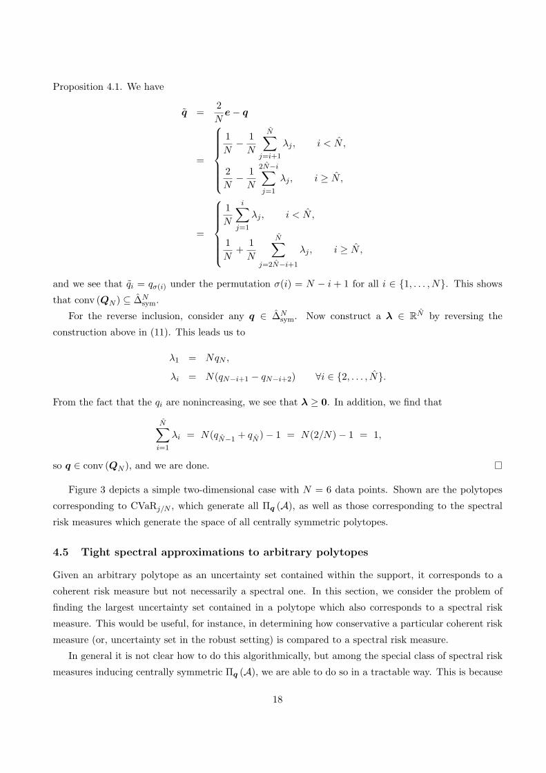
Proposition 4.1. For q ∈ ∆Nsym, Πq (A) is centrally symmetric through a = AeN for any A if and
only if
q = 2eN − qσ, (9)
where σ is a permutation and eN is the vector with 1/N at each entry.
Proof. Πq (A) is centrally symmetric if and only if every extreme point is centrally symmetric. An
extreme point of Πq (A) is of the form Aqσ′ for some permutation σ′. Letting δ = Aqσ′ −AeN , Πq (A)
is symmetric if and only if AeN −δ = 2AeN −Aqσ′ ∈ Πq (A) for every permutation σ′. Since this must
hold for any A, this true if and only if there exists a permutation σ′′ such that 2eN − qσ′ = qσ′′ for
every permutation σ′. Clearly, (9) implies this to be true. Conversely, choose σ′ as the identity, which
means q = 2eN − qσ′′ for some other permutation σ′′, which is the same as (9).
This motivates the following definition.
Definition 4.9. The symmetric restricted simplex in N -dimensions is denoted by ∆Nsym and defined by
∆Nsym =
q ∈ ∆N : q satisfies (9)
.
16

We now prove that, like the restricted simplex, ∆Nsym is generated by a finite family of spectral risk
measures.
Theorem 4.4. The class of spectral risk measures which generate centrally symmetric sets Πq (A) for
any A is equivalent to the class of risk measures
µλ(X) =N∑
j=1
λjµj(X) λ ≥ 0,
N∑
j=1
λj = 1,
where N = bN/2c+ 1 and µj(X) is the spectral risk measure µj(X) = −∑Ni=1 qj
i x(i) with
qji =
2/N if i < j,
1/N if j ≤ i ≤ N − j + 1,
0 otherwise.
(10)
Proof. We assume N is odd; the proof for N even is nearly identical with some small changes on
summation limits. We define the matrix QN ∈ RN×N by
QN =[q1 · · · qN
].
Analogous to Theorem 4.2, if we can show that the convex hull of the columns of QN is equivalent to
∆Nsym, we will prove the claim.
For one direction, consider an arbitrary convex combination λ ∈ RN of the columns of QN , i.e., a
vector q ∈ RN such that q = QNλ. Clearly q ≥ 0 and q sums to one. We find that
qi =
1N
+1N
N∑
j=i+1
λj , i < N,
1N
2N−i∑
j=1
λj , i ≥ N .
We see that we can rearrange this to find that
qN = λ1/N,
qN−i = qN−i+1 + λi+1/N 1 ≤ i ≤ N − 1, (11)
qN−i = qN−i+1 + λN−i+1/N 1 ≤ i ≤ N − 1,
from which it follows that qi ≥ qi+1 as well, so q ∈ ∆N . We now check the symmetry condition from
17
Proposition 4.1. We have
q =2N
e− q
=
1N− 1
N
N∑
j=i+1
λj , i < N,
2N− 1
N
2N−i∑
j=1
λj , i ≥ N ,
=
1N
i∑
j=1
λj , i < N,
1N
+1N
N∑
j=2N−i+1
λj , i ≥ N ,
and we see that qi = qσ(i) under the permutation σ(i) = N − i + 1 for all i ∈ 1, . . . , N. This shows
that conv (QN ) ⊆ ∆Nsym.
For the reverse inclusion, consider any q ∈ ∆Nsym. Now construct a λ ∈ RN by reversing the
construction above in (11). This leads us to
λ1 = NqN ,
λi = N(qN−i+1 − qN−i+2) ∀i ∈ 2, . . . , N.
From the fact that the qi are nonincreasing, we see that λ ≥ 0. In addition, we find that
N∑
i=1
λi = N(qN−1 + qN )− 1 = N(2/N)− 1 = 1,
so q ∈ conv (QN ), and we are done.
Figure 3 depicts a simple two-dimensional case with N = 6 data points. Shown are the polytopes
corresponding to CVaRj/N , which generate all Πq (A), as well as those corresponding to the spectral
risk measures which generate the space of all centrally symmetric polytopes.
4.5 Tight spectral approximations to arbitrary polytopes
Given an arbitrary polytope as an uncertainty set contained within the support, it corresponds to a
coherent risk measure but not necessarily a spectral one. In this section, we consider the problem of
finding the largest uncertainty set contained in a polytope which also corresponds to a spectral risk
measure. This would be useful, for instance, in determining how conservative a particular coherent risk
measure (or, uncertainty set in the robust setting) is compared to a spectral risk measure.
In general it is not clear how to do this algorithmically, but among the special class of spectral risk
measures inducing centrally symmetric Πq (A), we are able to do so in a tractable way. This is because
18

−2 −1 0 1 2−1
−0.5
0
0.5
1
ai,1
All
0 1/6 1/3 1/2 2/3 5/6 10
0.2
0.4
0.6
0.8
1
u
g(u)
Distortion functions
−2 −1 0 1 2−1
−0.5
0
0.5
1
ai,1
a i,2
Symmetric
0 1/6 1/3 1/2 2/3 5/6 10
0.2
0.4
0.6
0.8
1
u
g(u)
Distortion functions
Figure 3: For a case with N = 6 data points (denoted by ∗): the 6 basis generators for Πq (A) (upper left) and
the corresponding distortion (CVaRj/N ) functions (lower left); the 4 basis generators for the centrally symmetric
subclass of Πq (A) (upper right) and the corresponding distortion functions (lower right).
these risk measures naturally induce a norm, and thus provide a convenient way of approximating more
general measure structures, as we now illustrate.
We first describe the norm induced by the sets Πq (A), where q ∈ ∆Nsym.
Proposition 4.2. For a comonotone generator q ∈ ∆Nsym and any A, with a = AeN , the function
‖a− a‖q,A = inf
α > 0∣∣∣∣
a− a
α∈ πq(A)
, (12)
where πq(A) is Πq (A) shifted by −a, is a norm.
Proof. ‖ · ‖q,A is a form of a Minkowski function, and it is well-known that this function is convex
whenever the underlying set in question (here πq(A)) is closed and convex, which is the case in this
construction. Without loss of generality we assume a = 0 in the remainder of this proof.
‖a‖q,A = 0 implies that a/ε ∈ Πq (A) for all ε > 0. As Πq (A) is a bounded set, this can only be
the case if a = 0.
If β > 0, it is easy to see that ‖βa‖q,A = β‖a‖q,A by a simple scaling argument. If β < 0, we have
βa ∈ Πq (A) if and only if Πq (A) is centrally symmetric through zero; this is the case, however, since
q ∈ ∆Nsym. Combining all this, we see that ‖βa‖q,A = |β|‖a‖q,A.
19

Finally, noting that this function is convex, we have, for all a1,a2 ∈ Rn,
‖a1 + a2‖q,A = ‖2(.5a1 + .5a2)‖q,A
= 2‖.5a1 + .5a2‖q,A
≤ ‖a1‖q,A + ‖a2‖q,A,
which completes the proof that it is a norm.
The norm ‖ · ‖q,A has one particular property which is of interest.
Lemma 4.2. Let q ∈ ∆Nsym be any centrally symmetric generator and λ ∈ R. Then the vector q =
λq + (1− λ)eN satisfies
‖a − a‖q,A =1|λ|‖a − a‖q,A (13)
for all a ∈ Rn.
Proof. The proof follows by noting that Πq (A) is a scaled version of Πq (A) around a by a factor
of λ. Indeed, it is easy to see that the extreme points of Πq (A) affine combinations of the extreme
points of Πq (A) and eN (which is permutation-invariant). (Note that because of this we may as well
assume λ ≥ 0, as λ < 0 reflects the set through a, and it is centrally symmetric through this point by
construction.) The result then follows from the definition of ‖ · ‖q,A.
Now consider a robust optimization constraint with an arbitrary polytope U as the uncertainty set.
We assume that the sample mean a ∈ U . In particular, assume U has the form
U =a ∈ Rn : u′ia ≥ vi, i ∈ 1, . . . , m . (14)
In such cases, we can always find a spectral risk measure which leads to an inner approximation (a
less conservative uncertainty set) on the robust problem with U . We will find an inner approximation
which is centrally symmetric through a and use the norm ‖ · ‖q,A derived in Proposition 4.2 to measure
the quality of the approximation.
Lemma 4.2 immediately suggests a method for finding an inner approximation to an arbitrary
uncertainty polytope U : begin with a centrally symmetric generator q ∈ ∆Nsym and “mix” it with as
little of the generator eN such that the result is contained in U . From Lemma 4.2 the resulting Πq∗ (A)
will be the largest in the ‖ · ‖q,A sense among all such mixtures contained in U . We now show how to
compute this algorithmically via linear optimization.
Theorem 4.5. Given a centrally symmetric generator q ∈ ∆Nsym and an arbitrary polytope U ⊆ Rn
described by (14) such that a ∈ U , the centrally symmetric Πq (A) which is largest in the ‖ · ‖q,A sense
20

among all such Πq (A) ⊆ U is given by the solution to the linear optimization problem
maximize λ
subject to q = λq + (1− λ)e/N,
e′(sk + tk) ≥ vk ∀ k ∈ 1, . . . , m, (15)
sk,i + tk,j ≤ (u′kaj)qi ∀ (i, j) ∈ 1, . . . , N2, ∀ k ∈ 1, . . . , m,
in variables sk ∈ RN , k ∈ 1, . . . , m, tk ∈ RN , k ∈ 1, . . . , m, q ∈ RN , and λ ∈ R. Moreover, the
resulting approximating uncertainty set corresponds to a spectral risk measure if and only if the optimal
value λ∗ of (15) satisfies
λ∗ ≤ 11−Nqmin
. (16)
Proof. Consider a single inequality constraint u′a ≥ v. We have u′a ≥ v for all a ∈ Πq (A) if and only
if the optimal value of the problem
minimizeN∑
i=1
qi
N∑
j=1
(u′aj)yij
subject toN∑
i=1
yij = 1 ∀ j ∈ 1, . . . , N,
N∑
j=1
yij = 1 ∀ i ∈ 1, . . . , N,
yij ≥ 0, ∀ (i, j) ∈ 1, . . . , N2,
is no smaller than v. We note that this is optimization over a bounded, nonempty polyhedron and thus
by strong duality the optimal value of this problem equals the optimal value of its dual
maximize e′(s + t)
subject to si + tj ≤ (u′aj)qi ∀ (i, j) ∈ 1, . . . , N2.
It is then easy to see that Πq (A) ⊆ U if and only if there exist s1, . . . , sm, t1, . . . , tm such that
e′(sk + tk) ≥ vk ∀ k ∈ 1, . . . ,m,sk,i + tk,j ≤ (u′kaj)qi ∀ (i, j) ∈ 1, . . . , N2, ∀ k ∈ 1, . . . , m.
Now, to find the largest such Πq (A) ⊆ U in the ‖ · ‖q,A sense, we can, by Lemma 4.2, set q =
λq + (1− λ)eN and maximize λ, which leads us to the desired linear program. The bound (16) follows
by noting that in order for q to correspond to a spectral risk measure, it must have nonnegative
components.
21
−2.5 −2 −1.5 −1 −0.5 0 0.5 1 1.5 2−1
−0.5
0
0.5
1
−2.5 −2 −1.5 −1 −0.5 0 0.5 1 1.5 2−1
−0.5
0
0.5
1
−2.5 −2 −1.5 −1 −0.5 0 0.5 1 1.5 2−1
−0.5
0
0.5
1
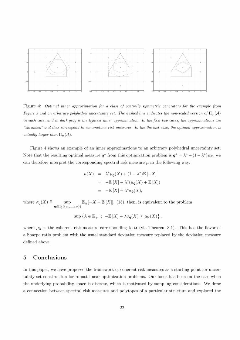
Figure 4: Optimal inner approximation for a class of centrally symmetric generators for the example from
Figure 3 and an arbitrary polyhedral uncertainty set. The dashed line indicates the non-scaled version of Πq (A)
in each case, and in dark gray is the tightest inner approximation. In the first two cases, the approximations are
“shrunken” and thus correspond to comonotone risk measures. In the the last case, the optimal approximation is
actually larger than Πq (A).
Figure 4 shows an example of an inner approximations to an arbitrary polyhedral uncertainty set.
Note that the resulting optimal measure q∗ from this optimization problem is q∗ = λ∗+(1−λ∗)eN ; we
can therefore interpret the corresponding spectral risk measure µ in the following way:
µ(X) = λ∗µq(X) + (1− λ∗)E [−X]
= −E [X] + λ∗(µq(X) + E [X])
= −E [X] + λ∗σq(X),
where σq(X) , supq∈Πq(e1,...,eN)
Eq [−X + E [X]]. (15), then, is equivalent to the problem
supλ ∈ R+ : −E [X] + λσq(X) ≥ µU (X)
,
where µU is the coherent risk measure corresponding to U (via Theorem 3.1). This has the flavor of
a Sharpe ratio problem with the usual standard deviation measure replaced by the deviation measure
defined above.
5 Conclusions
In this paper, we have proposed the framework of coherent risk measures as a starting point for uncer-
tainty set construction for robust linear optimization problems. Our focus has been on the case when
the underlying probability space is discrete, which is motivated by sampling considerations. We drew
a connection between spectral risk measures and polytopes of a particular structure and explored the
22
geometry and underlying generation of these classes of risk measures and corresponding uncertainty
sets.
Some interesting future directions are the following:
1. Multiple constraints and risk over vector spaces: Obviously we could apply our framework in a
constraintwise fashion, but there are undoubtedly more sophisticated ways to balance risk among
multiple constraints. It would be interesting to explore the resulting implications for robustness
under appropriately defined risk measures over more general vector spaces.
2. More general conic problems: We have restricted ourselves to linear optimization here. It is not
immediately clear how to extend this to more general robust optimization problems.
3. Integrating information beyond samples: How can we introduce additional knowledge of the dis-
tribution (e.g., prior distributions, bounds, or other constraints such as no-arbitrage conditions),
and what are the implications from the robust perspective?
Acknowledgements
We are grateful to two anonymous referees for a number of insights and observations which substantially
improved this manuscript.
References
[1] Acerbi, C. “Spectral measures of risk: A coherent representation of subjective risk aversion.” Journal of
Banking & Finance. 26:1505-1581, 2002.
[2] Acerbi, C. and Tasche, D. “On the coherence of Expected Shortfall.” Journal of Banking & Finance.
26(7):1487-1503, 2002.
[3] Artzner, P., Delbaen, F., Eber, J., Heath, D. “Coherent measures of risk.” Mathematical Finance, 9:203-228,
1999.
[4] Ben-Tal, A., Nemirovski, A. “Robust Solutions of Uncertain Linear Programs.” Operations Research Letters,
25(1):1-13, 1999.
[5] Ben-Tal, A., Nemirovski, A. “Robust Solutions of Linear Programming Problems Contaminated with Uncer-
tain Data.” Mathematical Programming, Ser. A, 88:411-424, 2000.
[6] Bertsimas, D., Lauprete, G.J., Samarov, A. “Shortfall as a risk measure: properties optimization, and appli-
cations.” Journal of Economic Dynamics and Control, 28(7):1353-1381, 2004.
[7] Bertsimas, D., Pachamanova, D., Sim, M. “Robust Linear Optimization under General Norms.” Operations
Research Letters, 32:510-516, 2004.
[8] Bertsimas, D., Sim, M. “Tractable Approximations to Robust Conic Optimization Problems.” Mathematical
Programming, 107(1-2):5-36, 2006.
23
[9] Calafiore, G., Campi, M.C. “Uncertain Convex Programs: Randomized Solutions and Confidence Levels.”
Mathematical Programming, Series A, 102(1):25-46, 2005.
[10] Chen, W., Sim, M., Sun, J., Teo, C.-P. “From CVaR to Uncertainty Set: Implications in Joint Chance
Constrained Optimization.” Working paper, 2007.
[11] Choquet, G. “Theory of capacities.” Ann. Inst. Fourier, pp. 131-295, 1954.
[12] Delbaen, F. “Coherent risk measures on general probability spaces.” In: Advances in Finance and Stochastics.
Essays in Honour of Dieter Sondermann, 1-37. Springer-Verlag, Berlin, 2000.
[13] Denneberg, D. “Distorted probabilities and insurance premium.” Methods Operations Research, 52:21-42,
1990.
[14] Dhaene, J., Denuit, M., Goovaerts, M.J., Kaas, R., Vyncke, D. “The Concept of Comonotonicity in Actuarial
Science and Finance: Theory.” Insurance: Mathematics & Economics, 31(2):133-161, 2002.
[15] El Ghaoui, L., Lebret, H. “Robust Solutions to Least-Squares Problems with Uncertain Data.” SIAM Journal
Matrix Analysis and Applications, 18(4): 1035-1064, 1997.
[16] El Ghaoui, L., Oustry, F., Lebret, H. “Robust Solutions to Uncertain Semidefinite Programs.” SIAM J.
Optimization, 9(1), 1998.
[17] Fischer, T. “Examples of coherent risk measures depending on one-sided moments.” Working paper,
http://www.ma.hw.ac.uk/∼fischer/papers/, 2001.
[18] Follmer, H., Schied, A. Convex measures of risk and trading constraints. Finance and Stochastics, 6(4):429-
447, 2002.
[19] Follmer, H., Schied, A. Stochastic Finance: An Introduction in Discrete Time. Walter de Gruyter, Berlin,
2004.
[20] Huber, P. Robust Statistics. Wiley, New York, 1981.
[21] Jouini, E., Medded, M., and Touzi, N. “Vector-valued coherent risk measures.” Finance and Stochastics,
8:531-552, 2004.
[22] Kusuoka, S. “On law invariant coherent risk measures.” Advances in Mathematical Economics, 3:83-95, 2001.
[23] Leitner, J. “A short note on second order stochastic monotonicity preserving coherent risk measures.” Math-
ematical Finance, 15(4): 649-651, 2005.
[24] Natarajan, K., Pachmanova, D., and Sim, M. “Constructing Risk Measures from Uncertainty Sets.” Working
paper, 2007.
[25] Nemirovski, A., Shapiro, A. “Convex Approximations of Chance Constrained Programs.” Working paper,
2006.
[26] Nemirovski, A., Shapiro, A. “Scenario Approximations of Chance Constraints.” Working paper, 2004.
[27] Queyranne, M. “An Introduction to Submodular Functions and Optimization.” Available at:
http://www.ima.umn.edu/optimization/seminar/queyranne.pdf. 2002.
24
[28] Rockafellar, R.T. and Uryasev, S.P. “Optimization of conditional value-at-risk.” The Journal of Risk. 2:21-41,
2000.
[29] Schmeidler, D. “Integral Representation without Additivity.” Proc. American Math Society, 97(2): 255-261,
1986.
[30] Soyster, A.L. “Convex Programming with Set-Inclusive Constraints and Applications to Inexact Linear
Programming.” Operations Research, 21(5):1154-1157, 1973.
[31] Wang, S. “A Class of Distortion Operators for Pricing Financial and Insurance Risks,” Journal of Risk and
Insurance, 67(1):15-36, 2000.
25