Construction of a consumption aggregate based on information from POF 2008-2009 and its

use in the measurement of welfare, poverty, inequality and vulnerability of families

Leonardo S. Oliveira*, Debora F. de Souza**, Luciana A. dos Santos*,

Marta Antunes*, Nícia C. H. Brendolin**, Viviane C. C. Quintaes **

Abstract

Given the complexity of family and individual welfare, this study aims to explain the

construction of a family consumption aggregate, using data from Brazilian Family Expenditure

Survey (2008-2009), and also to measure and analyze welfare, poverty, inequality and ulnerability.

Following the literature, some aspects were considered: the selection of expenditures, the analysis

of extreme values, the imputation of food consumption, the user cost of durable goods and a spatial

price deflator. After the definition of the family consumption aggregate, we analyzed the

Generalized Lorenz Curves, social welfare functions and inequality measures. Then we presented

the sensitivity of the identification exercise to different poverty lines and analyzed the severity of

poverty. Finally, based on Chaudhuri et al. (2002) and Elbers et al. (2002), the vulnerability to

poverty was studied taking account of area (clusters) effects. In this last exercise, the poverty line

was based on half the minimum wage in 2008.

Keywords: Social Welfare Functions, Inequality, Poverty Measurement, Error Component Models,

Heteroscedastic.

JEL: C21, D63, I32

* IBGE/DPE/COREN – Leonardo.s.oliveira@ibge.gov.br, Luciana.santos@ibge.gov.br, Marta.antunes@ibge.gov.br

** IBGE/DPE/COMEQ – Debora.Souza@ibge.gov.br; Nicia.Brendolin@ibge.gov.br; Viviane.Quintaes@ibge.gov.br

IBGE is exempt from any responsibility related to the opinions, information, data and concepts stated in this article that are of exclusive

responsibility of the authors.

The authors would like to thank Paulo Roberto Coutinho Pinto for his collaboration and Elisa L. Caillaux and Marina Aguas for their comments.

1

Introduction

The Brazilian Family Expenditure Survey (POF) provides information about the household

budget composition, consumer habits, expenditure and income distribution, household and people

characteristics. The data collection focus on expenditure and acquisition of goods and services. To

make a consumption aggregate, it is necessary to identify the components of current expenses

associated with consumption as well as the value of consumption associated with the ownership of

assets, which guarantee a flow of services for the consumption unit.1 Therefore, for assembling the

consumption aggregate through the POF 2008-2009, a number of decisions had to be taken based on

theoretical hypothesis and empirical results, as it is presented in Section 1.

The choice of using consumption for measuring welfare, poverty, inequality and vulnerability

of consumption units is justified by two issues.2 First, both income and consumption present a

variation over time but consumption tends to be less variable than income and to reflect the average

long term welfare more accurately (Deaton, 1997, Deaton and Zaidi, 2002, Haughton and Khandker,

2009). Income fluctuations do not replicate directly into consumption fluctuations because people

might adapt or use credit, get donations or sell their assets in order to keep their consumption standard.

Note that consumption units with restrict access to credit will face more difficulties to boost their

consumption. Even considering some consumption seasonal fluctuations, associated with holidays or

festivities, these are smoother when compared to the income fluctuations of consumption units,

especially when their members are self-employed workers or employees of the informal sector. Those

who work in agriculture sectors are subject to higher seasonal fluctuations in income than in

consumption because a bigger portion of their consumption comes from their own production and not

from the market.3 The action of asking informants to estimate the value of goods acquired outside the

market (donations, production for their own consumption or withdrawal from their own businesses)

in the survey allows the measurement of non-monetary consumption.4 If this non-monetary

consumption was not considered, there would be an underestimation of welfare and a super-

estimation of poverty.

Secondly, consumption reflects the value that people attribute to different goods and services

at their disposal: food consumption; durable goods; housing; healthcare, education and transportation

and other non-food items. In this process, the consumption units will base their choices on market

1 The Brazilian Family Expenditure Survey worked with the concept of Consumption Unit, which can be approximated to the idea of household

units or family. For further details, see IBGE (2008). The Brazilian Family Expenditure Survey has also investigated the self-perception of life

quality (POF questionnaire 6) and the characteristics of the nutritional profile in the Brazilian population (POF questionnaire 7). However, in

the present stage of the aggregate consumption construction these data will not be used. 2 Haughton and Khandker (2009) clearly emphasized that both consumption and income are imperfect proxies of utility once they exclude

important contributions to welfare such as publicly provided services and goods. Atkinson et al. (2002) highlighted that surveys on living

conditions measure expenditure but not consumption, that is to say, the amount spent by a consumption unit during the specific period of time

of the survey expenditure collection may differ from the effective consumption in the same period of time. This difference can be due, for

example, to the use of stock holdings. The same argument applies for durable goods (see Section 1.2). Limitations, criticism and alternatives

to the use of both expenditure (consumption) and income as welfare measures can be found in Sen (2004, 2008 and 2009), Kakwani and Silber

(2007 and 2008), Oliveira (2010) and in the Journal of Economic Inequality (2011). 3 Haughton and Khandker (2009) compared the welfare measurement through income, which they called “potential”, and through consumption,

which they called “result”. They stated that income tends to be more seasonal and underreported than consumption, reaching the same opinion

of Atkinson (1998), Deaton and Zaidi (2002) and OECD (2013). 4 The POF team evaluated and selected part of these data for imputation in order to assure consistency. Nevertheless, if informants were not

asked to estimate the value attributed to these goods, 100% of imputation would be needed.

2

prices and the possibility of substituting goods and services. As a result, the consumption aggregate

weights the different goods and dimensions by market prices. Furthermore, Ravallion (2011)

emphasized the role of prices in the definition of opportunity costs and marginal rates of substitution

as one of the major advantages of using consumption aggregates as welfare indicators.

An analysis of individual welfare based on a consumption aggregate has an implicit money

metric utility function5 that returns the necessary amount for keeping the consumption unit welfare

level and requires consumption to be adjusted by a price index. In order to do that, it is necessary to

construct price deflators that indicate life costs differences among distinct Brazilian geographical

contexts, as described in Section 1. In Section 2, an analysis of social welfare is performed using the

consumption aggregate constructed, in which the Generalized Lorenz Curve and (abbreviated) social

welfare functions based on Sen and Atkinson’s works are considered. To understand the weight of

inequality in the reduction of social welfare, two breakdowns are done: i) through the Gini index,

consumption inequality is broken down by component; and ii) through the mean logarithmic

deviation, inequality is broken down by population subgroups considering the years of education,

sex, color and race of the person responsible for the consumption unit. In Section 3, poverty and

vulnerability analyses are presented based on poverty curves, square poverty gap index (severity of

poverty) and the probability of a consumption unit becoming poor.

To make it easier to understand and/or reproduce the structure of the consumption aggregate,

we provide all the codes of POF items (Consumption Aggregate codes.xlsx) used for its construction

as support material. You can also find a database containing the variables to form the households

consumption unit's key used in POF 2008-2009 in addition to the consumption aggregate and the

spacial price deflator (database.csv). We provide, in the end of the paper in appendix 8, some

descriptive statistics and graphics comparing the consumption aggregate constructed in this paper

with the total expenditure identified by the survey (that includes all the monetary and non-monetary

acquisitions registered by POF) and the general consumption expenditure registered in POF (that

results from the total expenditure minus the items that represent patrimonial variation and other

recurrent expenses: taxes, labor deductions, bank services, pensions, allowances, donations and

private social security). An analysis of this material permits the identification of differences in the

distribution of these 3 welfare indicators as well as significant impact on the measuring of inequality

and poverty. Such differences behave as expected considering the way information was handled to

assemble the consumption aggregate, as described in the following sections.

1. Consumption aggregate

Assembling the consumption aggregate is a complex exercise that requires fine discrimination

between which expenses items might be included or not, so as to allow the comparison of the

consumption units’ welfare levels with its correct ranking. This discrimination is guided by applied

5 See Varian (1992, p.108-110) and Deaton and Zaidi (2002, p.4-13) to learn about the usefulness of the money metric utility and its relation

with other forms of measuring welfare.

3

literature and theoretical hypotheses about welfare contribution of different goods and services, as

well as by the necessary adaptations to the culture of the country under study.

Hentschel and Lanjow (1996) presented general principles to guide the construction of the

consumption aggregate and applied them to the poverty analysis in Ecuador. Slesnick (2001) studied

poverty and social welfare in the US and gave special attention to consumption and its components.

Lanjow and Lanjow (2001) analyzed the effect of the measurement error in consumption and

suggested the exclusion of some componentes in the welfare analysis. Deaton and Zaidi (2002)

advanced in the discussion about the consumption aggregate using family expenditure survey data of

eight countries. Haughton and Khandker (2009) also helped to disseminate steps used in the

construction and analyses of the consumption aggregate. Lanjow (2009) examined the Brazilian case

and recommended procedures to the inclusion of consumption items in the welfare analysis.These

autors suggested methodological ways to theoretical and practical problems faced in the construction

of such aggregates.

Considering the POF methodology, which measures expenses made per consumption unit by

type and in differentiated periods of time (7, 30 and 90 days and 12 months), some criteria needed to

be determined to deal with the information collected by the survey, adapting them to the consumption

aggregate construction. First, it was necessary to group the expenses of the different POF blocs into

consumption groups in order to select the ones that would compose the aggregate and the ones that

would be excluded. The following consumption groups were defined: food; durable goods; housing;

education, health and transportation; and other non-food items. Subsequently, each item of these

groups was analyzed as to verify if they complied with the following criteria:

(a) The item acquisition is not sporadic, i.e., it is frequently acquired in such a way that the

collection period of the survey is sufficient and does not distort the welfare analysis among

the consumption units. The durable goods whose acquisition tends not to occur annually

received a differentiated treatment (see Section 1.2).

(b) The item is acquired for the consumption unit own consumption, i.e., the acquisition of such

good will increase the welfare of the consumption unit under analysis and not that of another

unit.

(c) The item contributes to welfare comparability between different units and its corrected

ranking.

1.1. Food Expenditure

Food expenditures are obtained in the questionnaire “Collective Acquisition Booklet” (POF 3)

and in the bloc meals out-of-home (bloc 24) from the questionnaire “Individual Acquisition” (POF

4). The expenses with food were totally included, considering this is an important group when it

comes to measure the consumption units’ welfare (the share of food expenditures and other items in

the aggregate consumption are presented in section 2.3). It was found that 5.4% of the consumption

units presented null food expenditure. This can be explained by the reference time period of

4

information collection (7 days) that reported zero for consumption units that did not acquire food in

that week. In order to correct possible distortions in social welfare, inequality, poverty and

vulnerability due to these null food expenditures, an imputation was made following the Propensity

Score method. In this method, we estimate the probability of each consumption unit to have food

expenditure and we compare the consumption units with and without food expenditures using those

probabilities. In the end, the consumption units with food expenditure are used as donors of food

expenditure for the consumption units without food expenditures. For further details, see Rosenbaum

and Rubin (1983).

Appendix 1 shows the explanatory variables of the logit model applied and density functions of

the per capita consumption with and without food expenditure imputation.

1.2. Durable goods

The possession of durable goods has positive impacts over consumption units´ welfare.

However, while the acquisition of durable goods occurs in a particular point in time, its consumption

may occur during several years, as Haughton and Khandker (2009) and Atkinson (1998) pointed out.

There is difficulty in defining which goods might be considered durable, once, as Atkinson (1998)

explained, there is a durable element in several goods. In the construction of the consumption

aggregate, the following were considered as durable goods: “Main household durable goods

inventory” (bloc 14); “Machines, equipment and household utilities acquisition” (bloc 15); “Tools,

pets, musical instruments and camping gear acquisition” (bloc 16); “Furniture acquisition” (bloc 17)

and “Vehicles acquisition” (bloc 51). The exception were veterinarian services and expenses with

pets in bloc 16 that were included in the aggregate as other non-food expenses.

However, these durable goods had to be selected and treated before being included in the

aggregate. Following the suggestion made by Hentschel and Lanjow (1996), Slesnick (2001) Deaton

and Zaide (2002), ILO (ICLS 17- 2003), Haughton and Khandker (2009) and the OCDE (2013) guide

for household income, consumption and wealth statistics, the durable goods were included in the

consumption aggregate taking account of the value of services (not their value of acquisition), which

may be measured by the “user cost” or “rental equivalent” that the consumption unit “receives” for

all durable goods in its possession during a period of time of one year. This user cost value (UC) can

be approximated by:

𝑈𝐶𝑡𝑖𝑗 = 𝑆𝑡𝑖𝑗𝑃𝑡𝑖(𝑟𝑡 − 𝜋𝑡 + 𝜎𝑖) (1)

where Stij is the stock of the durable good i (quantity listed in the inventory) in the consumption unit

j during the survey period t; Pti is the current value of durable good i during the survey period t; rt is

the nominal interest rate; t is the inflation in the survey period t; and i is the depreciation rate of

the durable good i.

The depreciation rate is given by the following formula:

𝜎𝑖 − 𝜋𝑡 = 1 − (𝑃𝑡𝑖 𝑃𝑖(𝑡−𝑇𝑖)⁄ )1

𝑇𝑖⁄

(2)

where Ti is the lifetime of durable good i in years and Pi(t-Ti) is its price in the year it was acquired.

5

POF bloc 14 (“Main household durable goods inventory”) informs which goods are owned by

the consumption unit during POF collection period t and its stock St, as listed in the inventory.

Moreover, in relation to the last acquisition of these goods, it is possible to know the way it was

acquired, the year it was acquired and its condition, whether firsthand or secondhand. Thus, we have

the stock St and the lifetime of the item in years (T). The exception is for the secondhand goods, for

which there is only the last acquisition date. Therefore, in order to obtain the user cost for each good,

it is necessary to calculate the current prices of each good, the average nominal interest rate for the

POF time period and the regional deflators. These steps will be detailed below.

a) Median price calculation by Federative Unit (Pti UF)

Considering that through POF collected data it is not possible to calculate the current price of

each durable good, the solution was to estimate this through the calculation of the median price for

every durable good, by Federative Unit, using the information about the price of these goods in POF

bloc 15 (“Machines, equipment and household utilities acquisition”) and POF bloc 51 (“Vehicles

acquisition”). This calculation used only firsthand products prompt paid per Federative Unit. The use

of the median price aimed to minimize the outliers’ impact in each estimated price.

It must be highlighted that the only goods that had their prices studied were the ones that

appeared in POF bloc 14 (“Main household durable goods inventory”) and POF bloc 15 or POF bloc

14 and POF bloc 51, since it was necessary to match the information in stock and price. Therefore,

the goods that were not in the inventory but were present in bloc 15 were excluded from the

consumption aggregate. Their insertion would generate a distortion between the consumption units

that acquired durable goods during the period of the survey (from May, 2008 to May, 2009), which

would have a higher consumption aggregate, and the ones that acquired the same goods in another

time period not covered by POF, which would have a smaller aggregate.

For the calculation of durable good i current price (PtiUF), the median price of the Federative

Unit where the consumption unit locates was chosen. However, in some Federative Units there was

no acquisition of some specific goods according to previously established standards: goods acquired

firsthand and prompt payment. For these cases where it was not possible to calculate the median price

of the durable good i per Federative Unit, the median price of the good i of the corresponding Major

Region was used for the calculation of the user cost.

In a second exercise, we calculated the mean prices instead of median prices, reaching values

slightly larger due to the asymmetric distribution and possible outliers. Thus, we continued using the

median prices.

b) Mean nominal rate of interest calculation (rt)

Deaton and Zaidi (2002) suggested the use of one real interest rate only, based on an average

of several years for all durable goods. SELIC (Special System of Settlement and Custody) daily rate

information provided by the Brazilian Central Bank was used to calculate the average nominal interest

rate (1.1261), opting for the POF period – from May, 2008 to May, 2009.

c) Calculation of the average regionalized real interest rate of the period

6

For the calculation of the real interest rate, besides the average nominal interest rate the

inflation rate of the period was needed. Even though there is not available price index (IPCA)

information for all Federative Units, a deflator of a geographical area of influence was used where

such information was unavailable.

d) Depreciation rate ()

POF bloc 14 provided no information on the prices of goods when they were acquired

(Pi(t-Ti)). For this reason, an estimate of the depreciation rate had to be made, following the approach

suggested by Deaton and Zaidi (2002), learning from other countries experiences, such as: Vietnam,

Nepal, Ecuador and Panama.

The calculation of the mean usage time (𝑇𝑖) of durable goods acquired firsthand and prompt

paid is made by using the data of the year of acquisition registered in the inventory (POF bloc 14).

By usage time (T) we mean the difference of years between 2009 (top limit of the survey period) and

the year of acquisition (A) of the durable good i reported in the inventory of consumption unit j:

𝑇𝑖 = 𝑚𝑒𝑎𝑛(2009 − 𝐴𝑖𝑗) (3)

Also according to Deaton and Zaidi (2002) and Hentschel and Lanjow (1996) suggestions,

the mean useful lifetime of each durable good 𝐿𝑖 was considered as twice the mean usage time (T)

for each durable good, considering the sampling design of the survey:6

𝐿𝑖 = 2𝑇𝑖 (4)

We applied this for all durable goods listed in the inventory. We highlight that, only items in good

condition, functioning, or waiting for repairs for future use were listed in the POF’s inventory.

The depreciation rate is then calculated by the following formula:

𝜎𝑖 = 1/ 𝐿𝑖 (5)

For the durable goods that were not in the inventory and that were acquired by the

consumption unit during the 12 month period of the survey (POF blocs 16 and 17), there is no

information about the date of acquisition. As a result, the option was to exclude them, since they

were considered occasional expenses of the consumption units and their inclusion would introduce

a distortion in the welfare analysis.

A critical data review was made in order to verifiy if machines, equipments and household

utilities acquired during the survey period (POF bloc 15) were already part of the inventory (POF

bloc 14). It concluded that the number of goods in stock was higher than the number of durable

6 We checked if the estimated depreciation rates were in line with the Brazilian context. Then, these results were compared with the Regulatory

Instruction SRF number 162 from December 31, 1998, which establishes the useful lifetime and depreciation rate of goods related to the

Mercosur Common Nomenclature (MCN) and other goods. By these norms, we have an estimated useful lifetime of about 1.7𝑇. So using 2𝑇 looks reasonable for the Brazilian case since it points to a longer (but not so different) lifetime than the one in the Regulatory Instruction. Note

that the norm considers durable goods for commercial purposes and not durable goods acquired by a household consumption unit. Futhermore,

the use of 2𝑇 could be motivated by the hypothesis that the acquisitions are distributed in a uniform way over time and none of the inventory

items were recently introduced in the market. It must be noted that the mean time was calculated only for goods acquired new, once there is no

information about the real usage time for secondhand goods.

7

goods acquired for all consumption units. Therefore, the goods of POF bloc 15 could be excluded

without losing information on durable goods’ stock.

e) User Cost

After gathering all variables, the user cost of each durable good was calculated, according

to the formula below:

𝑈𝐶𝑡𝑖𝑗 = 𝑆𝑡𝑖𝑗𝑃𝑖𝑡𝑈𝐹𝑗(𝑟𝑡 − 𝜋𝑡𝑗 +

1

𝐿𝑖) (6)

where 𝑆𝑡𝑖𝑗𝑃𝑖𝑡𝑈𝐹𝑗 is the quantity of durable good i multiplied by its median price in the Federative

Unit7 where the consumption unit j is located; rt - tj is the regional real interest rate; and 𝐿𝑖= 2𝑇𝑖.

The results originated for the durable goods user cost per Federative Unit are available in Appendix

2.

1.3. Housing

The housing group had the biggest participation in the expenditure of Brazilian consumption

units across all income classes. For this reason, this group has relevance for the welfare analysis.

Items related to housing of the main household were classified in seven types of expenditure, which

are: rent, public services, household refurnishment, furniture and household goods, electrical

appliances, electrical appliances repairs and cleaning material.

Rental expenses were totally included. The inclusion of paid rent does not distort the

comparability between the consumption units, because POF investigated, for residence-owned

households, the estimated value of the amount that they would have to pay in case they were renting

it. Thus, families that own their estates were not measured with lower welfare in comparison with the

ones that pay rent.

Deaton and Zaidi (2002) also recommended including public services expenses (water,

sewage treatment, electricity, etc.) in the consumption aggregate. These services add welfare to the

consumption units. The inclusion or not of the items related to household refurnishment relates to the

possibility of finding if these expenses aggregate value to the household or not. In POF 2008-2009,

household maintenance expenses were considered for a period of 90 days and construction expenses

for a period of 12 monthsbut the later ended up being excluded from the consumption aggregate since

it aggregates value to the household. All expenditures with cleaning material were included because

they are recurrent expenses and increase the consumption units’ welfare.

1.4. Education, health and transportation

Healthcare expenses do not allow adequate measurement of welfare loss and gain associated to

them, once the healthcare expenses do not necessarily generate welfare gains - they can be mere ways

of minimizing welfare losses. For example, high healthcare expenditure on terminally ill patients

7 Remember that for some durable goods it was not possible to calculate the median price by Federative Unit for lack of information about the

acquisition of the referred good. In these cases, the median price of the corresponding Major Region was used.

8

cannot be compared to a surgery or treatment expenditures that contribute to recovering a patient, or

even to an aesthetic-cosmetic procedure.

Education expenditure may cause distortion due to the consumption unit age structure, because

it could be seen as an investment that usually occurs at the beginning of a person’s life cycle.

According to Lanjow (2009) and Deaton and Zaidi (2002), the decision to include healthcare

and education expenses should be considered in cases where these expenses elasticity (in relation to

the total expenditure) is above one. As pointed in Deaton and Zaide (2002), this procedure is similar

to the suggestion presented in Lanjouw and Lanjouw (2001) to deal with measurement errors in

expenditures (or welfare ranks). Thus, in order to decide about the inclusion or exclusion of these

items, an analysis of these expenditure elasticities was done.

As it can be observed in Table 1, education expenditure elasticity is above one, justifying the

total inclusion of these expenses in the aggregate (POF bloc 49). However, the healthcare elasticity

is 0.92, requiring a more detailed analysis of elasticity to decide on its inclusion or exclusion.Those

results are in line with Lanjow (2009), who estimated elasticities using data from POF 2002-2003.

Place Table 1 here

Table1: Elasticity of health and education expenditure

Considering the low values of elasticity of healthcare expenditure in all income classes, the

decision was for including solely the healthcare and dental insurance contracts (POF bloc 42) due to

their characteristic of providing welfare to the consumption units that access these services.

Furthermore, these expenses are responsible for a significant proportion of the consumption units’

current expenses.

Place Table 2 here

Table2: Elasticity of health expenditure versus total expenditure

by deciles of the per capita income distribution

Nordhaus and Tobin (1972) suggested the exclusion of commute expenses alleging that such

expenses do not directly contribute to welfare (utility), being "regrettably necessary inputs" to other

activities that generate welfare. This point is also mentioned in Stiglitz, Sen and Fitoussi (2009).

Deaton and Zaidi (2002) argued that the choice of an expenditure (or a high level of expenditure)

eliminates the "regrettable necessity" characteristic and reveals individual preferences. Deaton and

Zaidi (2002) suggested the inclusion of such expenses to the extent that it is represented consumption

and welfare for those who, by choice, live in nice places away from work ("pleasant suburb").

However, this example does not fit the Brazilian reality in most cases, since the remote locations are

often in need of many services.

Based on the arguments of those authors and the information in POF bloc 23, we chose to

exclude costs of mass transportation (bus, subway, train, ferry-boat, alternative transportation and

their connection), often used to go and return from work and often higher for those who live far away.

The low income elasticity of expenditure in transportation (0.61) also suggests that not all

transportation expenses must be considered in the calculation of consumption. We included

9

expenditure on one's own vehicle (fuel, parking, toll, and carwash), taxi, airplane and car rental

because, to some extent, those expenditures reflect individual choices and preferences.

Travel expenses (POF bloc 41) that are not motivated by business and professional reasons or

health treatment were included in the aggregate. This kind of information allows us to consider the

transportation expenses on leisure and to perform a differentiation of consumption units through

luxury goods expenses.

1.5. Other non-food goods

This group aggregates expenses related to clothing (except for the item wedding dress), culture

and leisure, personal services (manicurist, pedicurist, barber, hairdresser etc), hygiene and personal

care, smoking habits and other miscellaneous expenses. Among the miscellaneous expenses, we

considered expenses with other properties, parties, communication and professional services, such as

registry office, lawyer and forwarding agents. According to Haughton and Khandker (2009), wedding

and funeral expenses should not be considered in the consumption aggregate, as well as infrequent

and expensive acquisitions. Deaton and Zaidi (2002) have the same reading on the exclusion of these

items. From these, expenses related to ceremonies and parties were excluded due to their occasional

character and high values, and expenses with tickets for parties or social events were included. The

same was done with expenses related to games and professional services.

Frequent expenses with utilities (such as light, water, sewage, condominium fees, parking

spaces fees, etc) related to other properties of the consumption unit and used for their own benefit

(summer house, as an example) were included, while taxes, social contributions, pensions,

allowances, donations to other households and private social security taxes were excluded. The

banking expenses were included in the consumption aggregate except for the overdraft banking

services and credit card expenses.

1.6. Deflator

Aiming to ensure the comparability of the consumption aggregate among different geographical

spaces and price patterns, in the same period of time, a deflator was calculated using data from the

consumption units. In this calculation, we used the consumption units with incomes between the 2nd

and the 5th deciles as suggested by Ferreira, Lanjouw and Neri (2000). Excluding those consumption

units from the range made consumption baskets more homogeneous, preventing that the luxury goods,

with low frequency, or goods with excessive quantities interfere in the analysis.

The rationale was to create typical and comparable consumption baskets for each analyzed

geographical areas. To do so, we considered a subset of the consumption aggregate items found in all

areas, where only the essential expenses for the consumption units were selected for the deflator

calculation: electric power, water and sewage, gas and communication (landline phone, mobile

phone, paid TV and internet); housing expenses (rent and condominium); food expenses; personal

hygiene; cleaning material; and home maintenance.8

8 There is no data available for communication services quantity. Thus, it was used the ratio between the total number of people in consumption

units having expenses on communication services and the consumption unit total, by geographical area, to calculate an average quantity, since

10

For the spatial price analysis the choice was to use geographical contexts instead of Federative

Units. Studying prices behavior through geographical contexts minimizes distortions caused by

regional characteristics. As a result, according to POF sampling design particularities, it was possible

to have results for the following geographical strata: Metropolitan Areas (Belém, Fortaleza, Recife,

Salvador, Belo Horizonte, Rio de Janeiro, São Paulo, Curitiba and Porto Alegre) and Federal District;

non-metropolitan Urban Area and Rural Areas of each Major Region.

The information of the consumption baskets and prices allowed us to calculate spatial index for

each geographical context in many ways. For example, one could use a Laspeyres like price index,

as in Ferreira, Lanjouw and Neri (2000), or a Paasche index, as suggested by Deaton and Zaidi (2002).

Others could follow the purching power parities (PPP) literature that uses, for example, a combination

of Fisher index (in the Èltetö-Köves-Szulc method) or a Paasche like index (in the Geary-Khamis

method) to account for spatial prices differences.9

We calculated a Paasche spatial price index and used it in our analysis. Appendix 3 shows the

the Paasche index for each Geographical Context. We also calculated and provided (Deflator

codes.xlsx) a Laspeyres index similar to Ferreira, Lanjouw and Neri (2000) and a Fisher index taken

as the geometric mean of those two indexes. Those indexes had a similar behavior.

2. Analysis of social welfare and inequality based on aggregated consumption

The social welfare functions are usually defined in terms of utilities or in terms of the value of

consumption (or income). The social welfare functions that become the sum or the average of

individual utilities are called utilitarian. In this section, we work, at first, with the Generalized Lorenz

Curve, which allows, in some cases, ranking social welfare of an extensive class of functions (in this

case, strictly S-concaves and increasing functions).10 That is to say, one assumes that the social

welfare ascends due to the growth of consumption and Pigou-Dalton progressive transfers (when

consumption (income) is transferred from a richer to a poor person without turning the poor richer

than the one who transferred the consumption). Thus, the Generalized Lorenz Curve (GLC) will point

the social welfare in three Geographic Areas (Metropolitan area and Federal District, Urban Area and

Rural Area) and the Major Regions without the need to define a specific social welfare function.

In the second step of the analysis, one also assumes that the social welfare function is

homogenous at level 1 (or that there is a monotonous transformation that makes it homogeneous at

level 1). For this reason, it was possible to obtain (abbreviated) functions that show the effects of

inequality towards social welfare. This analysis was based on the Sen mean and the geometric mean

and also on their relations with Gini and Atkinson indexes for inequality.

it is common in Brazil to contract a package of those services for all the family members. The decision not to include information on estimated

rent in the housing category in the referred consumption basket is due to the fact that further study is needed in order to use it in the deflator. 9 A first presentation on life cost indexes can be found in Barbosa (1985). As Deaton and Zaidi (2002) stated, deflating consumption

expenditures by Laypeyres index yields an approximation of the welfare ratio whereas defacting by Paasche index yields an approximation of

the money metric utility. Blackorby and Donaldson (1987) and Ravallion (1998) suggested the use of the welfare ratio whereas Deaton and

Zaidi suggested the use of the money metric utility in welfare analysis. The Geary-Khamis and Èltetö-Köves-Szulc methods can be found in

Ackland, Dowric and Freynes (2007) or in the consumer price index manual (ILO 2004/2010). 10 The W(Xn) function is strictly S-concave when W(Xn.Anxn)>W(X) for any Xn that belongs to its domain and any matrix (Anxn) with non-

negative elements, having 1 as each line total and 1 as each column total. See Chakravarty (2009).

11

Once the loss of welfare due to inequality is described, the following constitutes a study of

inequality by components of the consumption aggregate, using the Gini index, and by subgroup of

the population, through mean logarithmic deviation.

2.1. Generalized Lorenz Curve

The GLC shows the population share (ordered from poorest to richest) on the horizontal axis

and shows the consumption partial mean times the population share on the vertical axis. When the

curve of an area is always above the other - as it occurs to the Metropolitan Area in Figure 1 - it is

noticed that there is Generalized Lorenz dominance (Foster et al., 2013, Chakravarty, 2009,

Shorrocks, 1983). The Metropolitan Area dominates the Urban Area and the latter dominates the

Rural. The conclusion is that any social welfare function that respects the criteria defined above will

maintain the social welfare hierarchy: higher welfare in the Metropolitan area, then in the Urban Area,

lastly in the Rural Area.

Place Figure 1 here

Figure1: Generalized Lorenz Curve and Generalized Lorenz Curve Differences (Area - Brazil) by Geographical Areas

In the analysis by Major Regions (Figure 2), the following welfare hierarchy is seen: South,

Southeast, Midwest, North and Northeast. It is noticeable that the GLC of Midwest is more similar

to the GLC of Brazil, which reflects a similar distribution in terms of consumption.

Place Figure 2 here

Figure 2: Generalized Lorenz Curve and Generalized Lorenz Curve Differences (Region– Brazil) by Major Regions

The GLC is important to establish the welfare hierarchy among the Geographical Areas and the

Major Regions. However, this analysis does not aim to provide a numerical value to social welfare

associated with each Geographical Area or Major Region or to measure the loss of welfare due to

inequality. To fill this gap, the following subsections will present two measures that permit the

measuring of welfare in terms of inequality and in terms of average consumption, respecting the

hierarchy found through the GLC.

2.2. Welfare and Inequality

In this section, one assumes that the function of social welfare is homogeneous at level 1 (or

that there is a monotonous transformation that makes it homogeneous at level 1). Thus, a proportional

increase in the consumption enhanced social welfare equivalently. Consequently, it is possible to

obtain (abbreviated) functions that show the effects of inequality on social welfare. This study is

based on the Sen mean and on the geometrical mean. More specifically, the Sen mean can be

described as the (abbreviated) Sen welfare function that depends on the average of per capita

consumption and on the Gini index (equation 7). Similarly, the geometric mean can be seen as a

12

(abbreviated) welfare function that depends on the average of per capita consumption and on the

Atkinson inequality index (equation 8).11

𝑊𝑆(𝑐) = ∑ ∑min{𝑐𝑖,𝑐𝑗 }

𝑁2𝑗𝑖 = 𝜇(1 − 𝐼𝐺) (7)

𝑊𝐺(𝑐) = (∏ 𝑐𝑖𝑖 )1

𝑁⁄ = 𝜇(1 − 𝐼𝐴) (8)

where ci is the consumption of the individual i; cj is the consumption of individual j; N is the total

population; IG is the Gini index; IA is the Atkinson index for inequality; and µ is the average of the

per capita consumption.

Table 4 shows the values of WS, WG, µ, IG and IA. As we can see, both the average of

consumption (µ) and the welfare measures (WS and WG) rank the geographical areas equally.

Moreover, as expected, the values of WS and WG are lower than the µ in all these areas. This

difference represents the loss of social welfare attributed to the inequality in the consumption. For

Brazil as a whole, the IG and the Sen measuring (WS) both indicate that half of welfare is lost due to

inequality of consumption. The Atkinson measure (IA) and the geometrical measure (WG) indicate a

loss of 36.0%. Another way of saying this is that the social welfare would be unchanged if the

consumption of families was reduced in 36.0% as long as it was distributed equally.

Place Table3 here

Table3: Mean per capita consumption, welfare functions and inequality indexes, by Geographical Areas and Major Regions

The other areas in Table 3 show similar results. Welfare losses between 43.0% and 51.0% by

the WS function and between 28.0% and 38.0% by the WG function.

Given the impact of social welfare inequalities, the following subsections will present two

decompositions: the first one by consumption aggregate components; and the second one by

subgroups of the population.

2.3. Decomposition of inequality by component of consumption

The decomposition of inequality by component of consumption is based on the fact that the

Gini index is the result of the concentration of each component of consumption and of the

participation of these components in the total consumption. As a result, it is possible to find out

which are the factors with higher contribution to the level of inequality.

Figure 3 shows the concentration curves of the five components used in the construction of the

consumption aggregate. The farther the curve is from the 45º line, the more concentrated the

11 WS can have different motivations. In general, one assumes that the contribution of consumption of one person (family) in social welfare

depends on his/her position (or ranking) in the consumption distribution. In some cases, the original welfare function value is identical to the

abbreviated function and to the equivalent consumption (Duclos and Abdelkrim, 2006). On this matter, see also Sen and Foster (1997) and

Lambert (2001). WG can be motivated by a logarithmic utility function and a social welfare function that consider the average of the utilities.

A monotonous transformation (the exponential of this function) generated the geometric average that assures the needed level 1 homogeneity.

One needs to highlight that the logarithmic utility function adopted is a particular case of utility function with constant elasticity, as presented

in Atkinson (1970). On this matter, see also Lambert (2001) and Duclos and Abdelkrim (2006)

13

component in analysis will be. Therefore, the biggest concentrations were in the consumption of the

groups “Education, health and transportation” and “Durable goods”. Remember that POF has no

information about the value of public education services or public health services. If those services

were taken into account, the group “Education, health and transportation” would be less concentrated.

The food group presented the lowest concentration and that is a coherent result since food

consumption is vital to living conditions.

Place Figure 3 here

Figure3: Concentration and Lorenz Curves, by component of consumption, Brazil

In Table 4, we see the results of the consumption aggregate decomposition with data for Brazil.

The product of the "consumption group participation" in the consumption aggregate and its

corresponding "concentration index" indicate the contribution of each component to inequality.12 It

is noticeable that the housing group had the highest participation in the total consumption, 32.2%. It

also had a high concentration (0.50), which makes this group the main responsible for inequality with

a relative contribution of 32%. The group "Education, Health and Transportation" was the most

concentrated of all the components and its concentration index reached 0.7. However, its relative

share in total consumption was small, 14.7%, making its relative contribution to inequality not the

greatest.

Place Table 4 here

Table 4: Index-Decomposition by component of consumption, Brazil

2.4. Decomposition of inequality by population subgroup

This subsection advances on the study of the decomposition of inequality by geographical area

and by characteristics of the person responsible for the consumption unit: years of education, sex, and

color or race. However, for the analysis of population subgroups, the Gini index was not used, since

it is not decomposable by subgroups in a way that one gets only the sum of the within inequality and

between inequality of the subgroups studied.

Thus, the decomposition by subgroups was made based on the mean logarithmic deviation

(ln(μ/WG)). This index belongs to the class of Generalized Entropy, closely associated with the

Atkinson measure of inequality. In the case of the mean logarithmic deviation index, this can be

described as the sum of inequality within each subgroup of the population, weighted by the share of

each subgroup, plus the existing inequality between the subgroups, see Lambert (2001) and Cowell

(2000) for further details on this index.

As we can see in Table 5, the inequality calculated by the mean logarithmic deviation for

Geographical Areas presented results similar to the level of Brazil (0.45), being of 0.47 in the

Metropolitan Region, 0.40 in Rural Areas, and 0.40 in Urban Areas. However, by having a greater

number of inhabitants (53.0%), the Urban Area, even with a lower level of inequality among the

12 A concentration index could also be broken in two parts: a "gini correlation index" and a “gini of the consumption component" so the product

of the "consumption group share" and those two parts yields the contribution of the consumption group to the total inequality. This other

decomposition can be found in Lerman and Yitzhaki (1985).

14

Geographical Areas, had a greater relative contribution (46.7%). Concerning the Major Regions, the

Southeast had the highest share of population and also the highest level of inequality (0.41). It may

be noted in this subgroup the cases of the Midwest and North regions, which have the smallest

population rates (7.3% and 8.0%, respectively), but a level of inequality rather high (0.40 and 0.38,

respectively).

Regarding the subgroup color or race, whites are responsible for the higher relative incidence

of inequality, 41.4%. Regarding the sex subgroup, the mean logarithmic deviation is very similar for

men (0.45) and women (0.45), i.e., the sex of the person responsible for the consumption unit did not

affect the consumption inequality. Therefore, the higher relative contribution of men to total

inequality is determined by their greater participation (72.4%) in the total number of persons

responsible for consumption units.

Place Table5 here

Table 5: Mean logarithmic deviation - decomposition by population subgroup

Through investigation of the results of the subgroup’s years of education, it is clear that there

was an inverse association between the number of years of education and the level of inequality, and

for the grades 8-10 years and 11-14 years the mean logarithmic deviation was stable and fell back

to people with 15 years or more of study.

Another way to examine the results of the mean logarithmic deviation was to look at the

interaction of inequality of subgroups with their weight in the population and the total inequality in

the country. As shown in Table 5, the main contribution to inequality in Brazil came from differences

within each subgroup. That is, although there was a Generalized Lorenz dominance of the

Metropolitan Area over the Urban and Rural Areas (see Subsection 2.1), 93.3% of Brazil's inequality

was explained by inequality within these subgroups. The same could be observed for subgroups of

the Major Regions (90.1%), and sex (99.9%). As it occurs in other studies, for example Ferreira et

al. (2006), most inequality comes from the differences within groups and not from the differences

between subgroups.

In the case of years of education and color or race, despite the importance of the within groups

inequality, the inequality between groups is, respectively, 31.5% and 12.4%. This makes years of

education extremely relevant to explain Brazil’s inequality.

The population could be divided into 5 subgroups, defined by the number of services to which

the consumption units (and its members) have access. More specifically, we considered access to

the following services: "water supply system", "sewage system", "electric supply system" and

"direct refuse collection". It was observed that a fraction of the population (1.8%) did not have any

of these services. A greater proportion (10.2% of the population) had only 1 of 4 services, usually

electricity services (97.8% of the cases); 11.9% of the population had only 2 services, the most

frequent pairs were electricity and water (49.9%) and electricity and refuse collection (48.3%). The

subgroup with 3 services corresponded to 30.4% of the population and the most frequent trio of

services were electricity, water and garbage collection (86.6% of cases). Only 45.6% of the

population had all 4 specified services.

15

For this reason, within each of those 5 subgroups, there was little variability in access to the 4

services selected. This picture contrasted with the existing consumption inequalities within the same

subgroups that ranged from 0.35 to 0.41 and contributed with 88.1% of the total consumption

inequality.

3. Analysis of poverty and vulnerability based on aggregated consumption

In this section, the consumption units are analised by Geographical Areas and subgroups of

population regarding poverty. In this sense, poverty measures that belong to the FGT (Foster, Greer

e Thorbecke, 1984) class were used with focus on poverty severity (FGT(2)). In order to estimate

the probability of a consumption unit becoming poor in a future period of time, a vulnerability

analysis based on Chaudhuri et al. (2002) methodology adapted to incorporate cluster effects was

done.

3.1. Poverty Severity

The consumption aggregate can also be used in studies of poverty from a monetary perspective.

Following this perspective, different dimensions (food, housing, education, health, transportation,

leisure etc.) were combined considering available prices and expenditure types as described in

previous sections. After calculating the consumption, two extra exercises were necessary in order to

evaluate poverty, the Identification and Aggregation exercises, emphasized by Sen (1976, 1982).

Besides the emphasis on these exercises, Sen’s studies comments the limitation concerning the most

used poverty measures at the time (that did not take inequality among the poor into account) and

stimulates an axiomatic approach in which poverty indexes are constructed to attend some properties

and evaluated by those properties. The Identification itemizes the poor and the non-poor, while the

Aggregation enables the combination of information about poverty in an index.

In general, the poor identification was based on some poverty line (z) that marked a limit to the

welfare indicator (in this case, consumption). The poor were identified by the welfare indicator

(consumption) that is below the line. The non-poor were identified by the indicator (consumption)

that is higher or equal regarding the poverty line13. In this work, two absolute lines were adopted

based on minimum wage. Consumption units with per capita income next to half of minimum wage

(between R$ 202.50 and R$ 212.50) and a quarter of a minimum wage (between R$ 101.25 and R$

106.25) were adopted. Then, the median per capita consumption of these two groups was calculated

resulting in two poverty lines based in consumption: R$ 185.00 and R$ 117.00.

In Figure 4, the proportions of the poor in Brazil are shown for the Geographical Areas and

Major Regions according to different poverty lines (R$ 1.00 ≤z≤ R$ 200.00). This helps one visualize

how sensitive the Identification exercise (of the poor) was towards the chosen lines. The inclination

of these curves around the lines R$ 185.00 and R$117.00 indicates this sensitivity. As it can be seen,

the sensitivity was higher in the Rural Area and in the North and Northeast regions. Even so, around

these two lines, we can see a clear hierarchy within the Geographical Areas and within the Major

13 Further details about different methodologies, definitions and interpretations regarding absolute, relative and subjective poverty lines can be

seen in Ravallion (2001), Soares (2009) and Atkinson et al. (2002).

16

Regions. That is to say that for an extensive set of lines next to R$ 185.00 and R$117.00 the proportion

of the poor was higher in the Rural Area followed by the Urban Area. Similarly, for an extensive set

of poverty lines next to R$ 185.00 and R$117.00 a bigger proportion of the population was classified

as poor in the North and Northeast and a smaller proportion in the South and Southeast.

Place Figure 4 here

Figure 4: Poverty curves by Geographical Area and Major Regions

Once the lines are selected, we move to the exercise of Aggregation, in which the information

about the poor is combined to analyze poverty in society. Three measures of the FGT family (Foster,

Geer and Thorbecke, 1984) were used to study poverty: the proportion or incidence of the poor [FGT

(α=0)], poverty intensity [FGT (α=1)] and poverty severity [FGT (α=2)], as defined in the expression

below:

𝐹𝐺𝑇 (𝛼) = 1

𝑛∑ [

𝑧−𝑦𝑖

𝑧]

𝛼𝑛𝑖=1 𝑆𝑖 (9)

where z is the poverty line value and Si is a dummy variable that is equal to 1 if the individual is

below poverty line and 0 otherwise. The bigger the coefficient α is, the bigger the poverty gap is.

The values of these measures for Brazil and Geographical Areas are presented in Appendix 4.

Among the three measures presented, only the one concerning poverty severity takes account

of consumption inequality among the poor. That is to say, keeping the total amount consumed by the

poor, the more heterogeneous the poor population is, the bigger the value of the indicator FGT(2).

That being said, this is the most appropriate poverty measurement, and that will be analyzed in Table

6.

Taking poverty severity by Geographical Area into consideration for the line R$ 185.00, it was

noticeable that poverty is more severe in the Rural Area (0.084). However, the Urban Area presented

the biggest relative contribution because of the weight of its population. When the same evaluation

was done with the line R$ 117.00, it was noticeable that the biggest contribution in terms of severity

comes from the Rural Area (45.2%), while the Urban Area represented 39,1%.

When poverty severity is analyzed by Major Regions taking the two poverty lines into account,

the Northeast presented the biggest poverty level, followed by the North. When one observes the

relative contribution, the Northeast still had the biggest participation.

In the subgroup related to color or race, it was recognizable that the black or mixed population

subgroups were the ones that most contribute to the severity of poverty, followed by the white

subgroup.

Place Table 6 here

Table 6: Poverty severity and relative contribution, by consumption lines,

according to Geographical Areas, Major Regions and Population subgroups

The results in Table 6 also show that poverty is more severe for people with no school education

or with only a few years of education (0-7 years), having a relative contribution of 87.2% (referring

to line R$ 185.00) and 88.7% (referring to line R$117.00) concerning poverty severity. In relation to

17

sex, there were no observed differences concerning poverty severity: referring to line R$ 185.00,

women had the index of 0.037 while men had 0.036; referring to line R$ 117.00, the values were

0.013 and 0.012, in the same order.

Considering again the services "water supply system", "sewage system", "electric supply

system" and "direct refuse collection", and separating the population into 5 subgroups (defined by the

number of services to which the CUs and their members had access) there was a clear association

between the severity of poverty and the number of services accessed. In this case, the subgroup

without access to any of the services was also the one that suffered more severely from poverty. The

lowest poverty rates were reported precisely by those with all four services. Together subgroups with

access to only one or none of the services were 12% of the population but accounted for about 33%

or 40% of poverty depending on the poverty line considered (R$185.00 or R$117.00, respectively).

3.2. Poverty vulnerability

Recent studies have emphasized the analysis of poverty vulnerability, understood as the chance

of the welfare indicator to present a value below the poverty line. Examples of this analysis can be

found in Lopes-Calvas and Ortiz-Juarez (2011), Ferreira et al. (2013), SAE’s Report (used it for the

definition of middle class) and Ribas (2007). A different approach can be found in Calvo and Dercon

(2008), which suggested a class of vulnerability index. It is important to highlight that the data set

that has a panel form is the most appropriate way to study vulnerability. However, Chaudhuri et al.

(2002) and Haughton and Khandker (2009) recommended the evaluation of vulnerability even in the

absence of data panels on consumption. In those cases, they suggested the use of regressions and

generalized least squares estimators to model the consumption distribution and the chance of a

consumption unit falling into poverty. In this section, the procedures of Chaudhuri et al. (2002) were

adapted to include area effects (clusters). Thus, a methodology similar to the one used in the Poverty

Map was applied (Elbers et al., 2002, IBGE, 2008).14

More specifically, the vulnerability of a consumption unit j to poverty in time t is defined as the

probability of the per capita consumption of that unit in time t +1 being below poverty line z:

𝜈𝑗𝑡 = 𝑃(𝑐𝑗,𝑡+1 < 𝑧) (10)

where 𝑐𝑗,𝑡+1 is the per capita consumption of the consumption unit j in time t+1 and z is the poverty

line calculated from the consumption aggregate.

One defines 𝑦𝑑𝑗 as a welfare variable function, being the logarithm of the per capita

consumption aggregate, of consumption unit j in the enumeration area d. The model can be written

as follows:

𝛾𝑑𝑗 = 𝑥𝑑𝑗𝛽 + 𝜂𝑑𝑗,𝜂𝑑𝑗 ~𝐹(0, 𝛴) (11)

meaning F is a distribution with a vector of average 0 and variance-covariance matrix 𝛴 and 𝑥𝑑𝑗 is

the vector of explanatory variables of the sample survey, regarding the consumption unit j of

enumeration area d, 𝑗 = 1, . . . , 𝑁𝑑 and 𝑑 = 1, . . . , 𝐷. It is possible to introduce indicators on

geographical levels that are more aggregated in order to control the area effect whenever it is not

14 Another possibility that might be explored in the future is the use of pseudo-panels as suggested by Bourguignon et al. (2006) and Dang and

Lanjouw (2013).

18

entirely explained through regressors. Such indicators can be obtained in other databases.

The model error may have two components: (i) unit effect associated with consumption unit;

and (ii) area effect associated with the enumeration area where this unit is placed. As a result, 𝜂𝑑𝑗 can

be written as:

𝜂𝑑𝑗 = 𝑢𝑑 + 𝑒𝑑𝑗 (12)

where 𝑢𝑑 and 𝑒𝑑𝑗 are independent from 𝑢𝑑~𝑁(0, 𝜎𝑢2) and 𝑒𝑑𝑗~𝑁(0, 𝜎𝑒𝑑𝑗

2 ).

Assuming that the errors of the unit level 𝑒𝑑𝑗 are heterocedastics, Elbers et al. (2002) suggested

estimating the logistic regression:

ln (𝑒𝑑𝑗

2

𝐴−𝑒𝑑𝑗2 ) = 𝑧𝑑𝑗

′𝛼 + 𝑟𝑑𝑗 (13)

and they estimated the variance on consumption unit level according to the formula:

�̂�𝑒𝑑𝑗

2 ≈ [𝐴𝐵

1+𝐵] +

1

2𝑣𝑎𝑟(𝑟) [

𝐴𝐵(1−𝐵)

(1+𝐵)3] (14)

where 𝐴 = 1.05𝑚𝑎𝑥(𝑒𝑑𝑗2 ); 𝐵 = exp(𝑧𝑑𝑗

′ �̂�), var(r) is the quadratic error of the estimated logistic

regression’s residual; and 𝑧𝑑𝑗 is a vector of explanatory variables.

Assuming that 𝑢𝑑 and 𝑒𝑑𝑗 have a normal distribution, Elbert et al. (2002) derived an estimate

of the area effect variance 𝑢𝑑:

𝑣𝑎𝑟(�̂�𝑢2) ≈ ∑𝑑2 {𝑎𝑑

2[(�̂�𝑢2)2 + (�̂�𝑑

2)2 + 2�̂�𝑢2�̂�𝑑

2] + 𝑏𝑑2 (�̂�𝑑

2)2

𝑛𝑑−1} (15)

where �̂�𝑑2 =

1

𝑛𝑑(𝑛𝑑−1)∑𝑗

(𝑒𝑑𝑗 − 𝑒𝑑.)2, 𝑒𝑑. =

1

𝑛𝑑∑𝑗

𝑒𝑑𝑗,𝑎𝑑 =𝑤𝑑

∑𝑗

𝑤𝑗(1−𝑤𝑗),𝑏𝑑 =

𝑤𝑑(1−𝑤𝑑)

∑𝑗

𝑤𝑗(1−𝑤𝑗) ,

�̂�𝑢2 = ∑

𝑑𝑎𝑑𝜂𝑑.

2 − ∑𝑑

𝑏𝑑�̂�𝑑2, 𝜂𝑑.

2 = 𝑢𝑑 + 𝑒𝑑., 𝑤𝑑 = ∑𝑗

𝑤𝑑𝑗

𝑛𝑑 and 𝑛𝑑 it is the total number of people associated

with the enumeration area d and 𝑤𝑗 is the survey expansion factor of the consumption unit j.

From the estimates found for the modeling procedure parameters, it is estimated the welfare

variable and the vulnerability of each consumption unit according to the equation:

�̂�𝑑𝑗 = 𝛷 (ln𝑧−�̂�𝑑𝑗

√�̂�𝑢𝑑2 +�̂�𝑒𝑑𝑗

2) (16)

Once the methodology is defined, the following step is the estimation of the consumption units

(and their components) vulnerability. As explanatory variables, data regarding consumption units

from POF were used, such as logarithm of available per capita monetary income, number of residents

per room, logarithm of total number of residents, indicator of bathroom, indicator of the geographical

context, some indicators about of the person responsible for the consumption unit such as literacy,

occupation, education, some enumeration area data such as the proportion of consumption units

whose heads had healthcare insurance and data on a municipal level from other sources, for instance,

the logarithm of per capita GDP in 2010 and the proportion of people who received Bolsa Família in

2010. The significance level concerning the choice of the variables was 0.05. See Appendices 5 and

19

6 for a complete list of the explanatory variables of the model and the estimated coefficient vectors α

and β.

It is important to mention that the variables selection aim was to select a model with good

predictive power without the pretension of presenting causal effects. The model adjustment (equation

11) resulted in a 𝑅2 of 0.75.

According to Chaudhuri et al. (2002), the consumption units with vulnerability index higher

than 0.5 were considered highly vulnerable. The expected consumption of these consumption units

and their components were below poverty line. It is possible that these consumption units end up

suffering from chronic poverty. The consumption units (and their components) with probabilities

between 0.2 and 0.5 were classified as vulnerable due to the fact that they presented estimated

consumption above the poverty line, but they still have big chances of falling into poverty. It is

possible that these consumption units may suffer from transitory poverty.15

Figure 5 indicates the relation between income and consumption vulnerability in a synthetic

way. More specifically, it indicates the average vulnerability (of per capita consumption) by

percentiles of per capita income and their respective confidence intervals of 95.0%. A strict relation

is observable between these incomes and the consumption units’ vulnerability. Around 16.0% of the

population presented average vulnerability higher than 0.5 and per capita income below R$ 181.70.

Thus, a rather low per capita income (less than R$ 181.70) also indicates high vulnerability (of

consumption). Similarly, per capita incomes between R$181.70 and R$ 327.24 can be considered a

sign of vulnerability (between 0.2 and 0.5). People who presented estimated vulnerability between

0.2 and 0.5 may face a situation of transitory poverty; they represent 19% of the Brazilian population.

Place Figure 5 here

Figure 5: Estimated average vulnerability by percentiles of per capita income

and their respective confidence intervals of 95%

Figure 6 indicates the estimated proportion of people vulnerable to poverty according to

different vulnerability threshold levels established between zero and one by (a) Metropolitan, Urban

and Rural Areas and (b) Major Regions. Among all levels of vulnerability thresholds, the North and

the Northeast regions presented bigger estimated proportions of vulnerable people, and the same

situation was observed in the Rural Area. The South region line decay is more accentuated than in the

other regions.

Place Figure 6 here

Figure 6: Estimated proportion of people vulnerable to poverty according to vulnerability threshold levels established

between 0 and 1.

In conclusion to the regional analysis, Figure 7 indicates the estimated proportion of people

vulnerable to poverty versus the estimated proportions of the poor estimated directly in POF for the

15 A more appropriate explanation concerning chronic poverty, as well as transitory, would also need data panels. See, for example, Ravallion

and Jalan (2000), Addison et al. (2009) and the Journal of Economic Inequality 10 (2012).

20

20 geographical contexts that compose the Geographical Areas and the Major Regions. Figure 7-a

focuses on highly vulnerable people (vulnerability above 0.5), while Figure 7-b focuses on vulnerable

people (vulnerability between 0.2 and 0.5). In Figure 7-a, we can observe that the contexts in the

North and Northeast regions present proportions of highly vulnerable people, higher than the

proportions identified for Brazil (horizontal line) - except for the Belem metropolitan region

(represented in one of the Urban Area contexts of the North region). The same occurred with the

estimated proportion of poor people in Brazil (vertical line). It is highlighted that, among Rural Areas,

the South was the only region that had a proportion of highly vulnerable people, lower than the

proportion identified for Brazil. The same tendency could be seen in (b).Therefore, people from the

South region and from Urban Areas of Southeast and Midwest regions are less vulnerable to poverty

than people from the North and from the Northeast regions.

Two other remarkable factors are related to the 45º straight line in these figures. As it is

observable, the proportion of highly vulnerable people was (fairly always) a little smaller than the

proportion of the poor, although these two measures behaved the same way. This can be explained

due to the fact that the proportion of the poor is a measure of (unconditional) vulnerability of society.

In Figure 7-b, the biggest differences could be seen since an increase of the proportion of poor was

not always followed by a similar increase in the vulnerability proportion.16

Place Figure 7 here

Figure 7: Estimated proportion of people vulnerable to poverty versus the estimated proportions of the poor calculated

directly from POF by the 20 geographical contexts which take part in Geographical Areas, and in Major Regions

4. Final considerations

The present article was proposed to examine the welfare, inequality, poverty and vulnerability

to poverty of Brazilian families from the perspective of consumption. This issue is commonly

addressed through the income perspective. However, the consumption pattern is brought as the most

suitable for these studies, since it presents a better response to seasonal fluctuations, demonstrating

how families behave according to their budget availability and, thus, better capturing their living

conditions.

The Brazilian Family Expenditure Survey (POF), conducted by IBGE, is the research that raises

the information expenses of a range sufficient to determine the consumption pattern of Brazilian

families. Nevertheless, the use of information from POF to conduct analysis on welfare, inequality,

poverty and vulnerability to poverty can be further investigated. For this reason, we selected no

sporadic expenses most likely to represent welfare gains and assigned values to the consumption of

durable goods by an estimate of the user costs. The last step of the consumption aggregate consisted

of correcting the values obtained by means of a spatial price deflator. As a result, we verified in this

paper that through the construction of a consumption aggregate, which reflects multiple dimensions

of the families consumption choices, such as food, housing, durable goods, health, education and

transportation and other non-food items, it is possible to perform these studies with POF data.

16 See Appendix 7: Estimated proportion of people vulnerable to poverty versus the estimated proportions of the poor calculated directly

from POF by the 20 geographical contexts, which take part in Geographical Areas and Major Regions.

21

Once defined the consumption aggregate, we advanced with the measurement of welfare,

poverty, inequality and vulnerability. To do so, we examined the behavior of the Generalized Lorenz

Curve, two (abbreviated) social welfare functions, we calculated Gini and Atkinson measures of

inequality and mean logarithmic deviation, then we decomposed inequality by components and by

population subgroup. To measure poverty, we analyzed the sensitivity of the exercise of identification

to the different poverty lines, and we presented the results of the poverty severity per geographic areas

and different population subgroups.Among the subgroups analyzed, we highlight that the difference

in years of education had a fundamental role for both inequality and poverty.

Finally, we assessed the vulnerability to poverty, including area effects (clusters) based on the

work of Chaudhuri et al. (2002) and Elbers et al. (2002).

We emphasize that the present paper is part of a larger work of poverty studies based on POF

data. Possible extensions of this study are, among other exercises, to apply the evaluation measures

and analysis presented here in other geographical divisions, the comparison of indicators over time

(2002-2003 and 2008-2009), the creation of pseudo panels to improve the measurement of

vulnerability and further study on the poverty lines.

5. References

Ackland, R., Dowrick, S. and Freyens, B., Measuring Global Poverty: Why PPP Methods Matter,

mimeo, Research School of Social Sciences, The Australian National University, 2007.

Addison, T., Hulme, D. and Kanbur, R., Poverty Dynamics: Interdisciplinary Perspectives, New

York, Oxford University Press, 2009.

Atkinson, A. B., “On the Measurement of Poverty”, Journal of Economic Theory, 2, 244-263, 1970.

______, “Lecture 1. Political Arithmetic: Financial Poverty in the European Union”. Poverty in

Europe, 10-66, YrjöJahnsson Foundation, 1998.

Atkinson, A., Cantillon, B., Marlier, E. and Nolan, B., Social Indicators: The EU and social inclusion,

New York, Oxford University Press, 2002.

Barbosa, F., Microeconomia: teoria, modelos econométricos e aplicações à economia brasileira, Rio

de Janeiro, IPEA, 1985.

Blackorby, C. and Donaldson, D., “Welfare ratios and distributionally sensitive cost-benefit

analysis”, Journal of Public Economics, 34, 265-290, 1987.

Bourguignon, F., Goh, C. and Kim, D., “Estimating Individual Vulnerability to Poverty with Pseudo-

Panel Data” in Morgan, S., Grusky, D. and Field, G., ed., Mobility and Inequality, 349-369,

Stanford, Stanford University Press, 2006.

Calvo, C., Dercon, S., “Risk and Vulnerability to Poverty” in Kakwani, N., Silber, J., ed., The Many

Dimensions of Poverty, 215-228, New York, Palgrave Macmillan, 2008.

Chakravarty, S. “Inequality, Polarization and Poverty: Advances in Distributional Analisys”,

Economic Studies in Inequality, Social Exclusion and Well-Being (vol. 6), New York,

Springer, 2009.

Chaudhuri, S., Jalan, J. and Suryahadi, A., “Assessing household vulnerability to poverty from cross-

sectional data: a methodology and estimates from Indonesia”. Discussion Paper 102,

NewYork, Economics Department, Columbia University, 2002.

Cowell, F. “Measurement of inequality” in Atkinson, A.B. and Bourguignon, F., (ed.), Handbook of

Income Distribution, 87-166, Amsterdam, Elsevier, 2000.

Dang, H-A. and Lanjouw, P., “Measuring Poverty Dynamics With Synthetic Panes Based on Corss-

Sections”, Policy Research Working Paper 6504, Washington DC, The World Bank, 2013.

22

Deaton, A., “6. Saving and consumption smoothing” The analysis of household surveys: a

microeconometric approach to development policy, 335-400, World Bank, The Johns Hopkins

University Press, 1997.

Deaton, A. and Zaidi, S., “Guidelines for Consctructing Consumption Aggregates for Welfare

Analysis”, Living Standards Measurement Survey Working Paper 135,Washington DC, The

World Bank, 2002.

Duclos, J–Y., Abdelkrim, A. “Poverty and Equity: Measurement, Policy and Estimation with DAD”,

Economic Studies in Inequality, Social Exclusion and Well-Being (vol. 2), New York,

Springer, 2006.

Elbers, C., Lanjouw, J. O. and Lanjouw, P., “Micro-level estimation of welfare”, Policy Research

Working Paper no. WPS 2911, Washington DC, The World Bank, 2002.

Ferreira, F. G. H., Lanjouw, P. and Neri, M., “A New Poverty Profile for Brazil Using PPV, Pnad

and Census Data”, Texto para Discussão, PUC-Rio, 418, 1-66, 2000.

Ferreira, F. G. H., Leite, P., Litchfield, J. A. and Ulyssea, G., “Ascensão e queda da desigualdade de

renda no Brasil”, in Barros, R., Foguel, M. and Ulyssea, G., Desigualdade de Renda no Brasil,

357-378, IPEA, 2006.

Ferreira, F. G. H., Melissa, J., Rigolini, J., Lopez-Calva, L., Lugo, M. and Vakis, R., Economic

Mobility and the Rise of the Latin America Middle Class, Washington DC, The World Bank,

2013.

Foster, J., Greer, J. and Thorbecke, E. “A class of decomposable poverty measures”, Econometrica,

52 (3), 761-766, 1984.

Foster, J., Seth, S., Lokshin, M. and Sajaia, Z., A Unified Approach to Measuring Poverty and

Inequality Theory and Practice, Washington DC, The World Bank, 2013.

Haughton, J. and Khandker, S., Handbook on Poverty and Inequality, Washington DC, The World

Bank, 2009.

Hentschel, J. and Lanjouw, P., “Constructing an indicator of consumption for the analysis of poverty:

principles and illustrations with reference to Ecuador”. LSMS Working Paper – Number 124,

Washington DC, The World Bank, 1996.

IBGE, Mapa de Pobreza e Desigualdade: municípios brasileiros 2003. Rio de Janeiro, IBGE, 2008

(CD-ROM).

______, Pesquisa de Orçamentos Familiares 2008-2009: Despesas, Rendimentos e Condições de

Vida, Rio de Janeiro, 2010.

ILO, Household income and expenditure statistics, Report II, Seventeenth International Conference

of Labour Statisticians, Geneva, December, 2003.

______, Consumer Price Index Manual: Theory and practice, 2004 (revisions as at 15/08/2010)

http://www.ilo.org/public/english/bureau/stat/guides/cpi/.

Journal of Economic Inequality, Special Issue: Inequality, New Directions. 9 (3), 1569-1721 (Print),

1573-8701 (Online), September, 2011.

______, 10 (2), 137-297, May, 2012.

Kakwani, N. and Silber, J. (ed.), The Many Dimensions of Poverty, New York, Palgrave Macmillan,

2007.

______, Quantitative Approaches to Multidimensional Poverty Measurement, New York, Palgrave

Macmillan, 2008.

Lambert, P., The Distribution and Redistribution of Income. New York, Manchester University Press,

3rd ed, 2001.

Lanjouw, J. and Lanjouw, P. “How to compare apples and oranges: poverty measurement based on

different definitions of consumption”, Review of Income and Wealth, 47 (1), 25-42, 2001.

Lanjouw, P, Constructing a Consumption Aggregate for the Purpose of Welfare Analysis: Principles,

Issues and Recommendations Arising from the case of Brazil, Paris, OECD Conference, 2009.

23

Lerman, R. and Yitzhaki, S., “Income Inequality Effects by Income Source: A New Approach and

Applications to the United States”, The Review of Economics and Statistics, 67, 1 (Feb., 1985),

151-156, 1985.

Lopez-Calva, L adn Ortiz-Juarez, E., “A Vulnerability Approach to the definition of the Middle

Class”, Policy Research Working Paper 5902, Washington DC, The World Bank, 2011.

OECD, OECD Framework for Statistics on the Distribution of Household Income, Consumption and

Wealth, 2013.

Oliveira, L. Três Ensaios Sobre Pobreza Multidimensional, Rio de Janeiro, UFRJ, Tese de

Doutorado, 2010.

Nordhaus W., Tobin J., “Is Growth Obsolete”, in ______, Economic Research: Retrospect and

Prospect, 5, 1-80, Economic Growth, NBER, 1972.

Ravallion, M. “Poverty Lines in Theory and Practice”. LSMS Working Paper – Number 133.

Washington DC, The World Bank, 1998.

______, Setting Poverty Lines: Economic Foundations of Current Practices, Washington,

Development Research Group, World Bank, 2001.

______, “On multidimensional indices of poverty”. Journal of Economic Inequality, 9, 235-248,

2011.

Ravallion, M and Jalan, J., “Is Transient Poverty Different? Evidence for Rural China”, Journal of

Development Studies, 36 (6), 82-99, 2000.

Ribas, R., Vulnerabilidade à pobreza no Brasil: Medindo Risco e Condicionalidade a partir da

Função de Consumo das Famílias, PPE, 37 (2), 2007.

Rosenbaum, Paul R. and Rubin, Donald B., “The central role of the propensity score in observational

studies for causal effects”. Biometrika, 70(1), 41-55, 1983.

SAE, Comissão para Definição da Classe Média no Brasil, Secretaria de Assuntos Estratégicos,

Brasil, 2011.

SEN, A. “Poverty: An Ordinal Approach to Measurement”, Econometrica, 44 (2), 219-231, 1976.

______, Poverty and famines an essay on entitlement and deprivation. Oxford, Claredon Press, 1982.

______, Desenvolvimento como Liberdade, São Paulo, Companhia das Letras, 2004.

______, Desigualdade Reexaminada, 2ª ed., Rio de Janeiro, Editora Record, 2008.

______, The Idea of Justice, Cambridge, Belknap Harvard University Press, 2009.

Sen, A and Foster, J., "On Economic Inequality after a Quarter Century", Annex to the enlarger

edition of On Economic Inequality by Sen, A., New York, Oxford University Press, 1997.

Shorrocks A., Ranking income distributions, Econometrica, 50, 3-17, 1983.

Slesnick, D., Consumption and Social Welfare: Living standards and their distribution in the United

States, Cambridge University Press, 2001.

Soares, S., Metodologias para estabelecer a linha de pobreza: objetivas, subjetivas, relativas e

multidimensionais, Rio de Janeiro, IPEA, Texto para Discussão 138, 2009.

SRF. Instrução Normativa da Secretaria da Receita Federal nº 162 de 31 de dezembro de 1998,

disponível em http://www.receita.fazenda.gov.br/Legislacao/ins/Ant2001/1998/in16298.htm,

acessado em 04/06/2013.

Stiglitz, J. E., Sen, A. and Fitoussi, J.P., Report by the Commission on the Measurement of Economic

Performance and Social Progress, 2009.

Varian, H., Microeconomic Analysis, New York, W. W. Norton & Company, Inc. (3rd edition), 1992.

24

Tables:

Table 1: Elasticity of health and education expenditure

Source: IBGE, Research Directory, Brazilian Family Expenditure Survey POF -2008-2009.

Note: For the calculation, the sampling design of the survey was considered.

Table 2: Elasticity of health expenditure versus total expenses by deciles of the per capita income distribution

Source: IBGE, Research Directory, Brazilian Family Expenditure Survey POF -2008-2009.

Note: For the calculation, the sampling design of the survey was considered.

Variable Elasticity Standard Error t Value P-value

Education * Expenses 1.20 0.0200 59.96 <0.0001

Education * Income 1.05 0.0203 52.04 <0.0001

Health * Expenses 0.92 0.0122 75.51 <0.0001

Health * Income 0.83 0.0110 75.48 <0.0001

Deciles

of incomeElasticity

Standard

Errort Value P-value

Consumption

units

1º 0.75 0.0430 17.37 <0.0001 5695

2º 0.72 0.0429 16.71 <0.0001 5552

3º 0.72 0.0381 18.85 <0.0001 5407

4º 0.75 0.0369 20.4 <0.0001 5263

5º 0.68 0.0339 19.92 <0.0001 5118

6º 0.63 0.0411 15.23 <0.0001 4759

7º 0.67 0.0445 15.01 <0.0001 4501

8º 0.83 0.0505 16.38 <0.0001 4073

9º 0.77 0.0416 18.46 <0.0001 4038

10º 0.73 0.0388 18.84 <0.0001 3480

25

Table 3: Mean per capita consumption, welfare functions and inequality indexes, by Geographical Areas and Major Regions

Source: IBGE, Research Directory, Brazilian Family Expenditure Survey POF -2008-2009.

Table 4: Index-Decomposition by component of consumption, Brazil

Source: IBGE, Research Directory, Brazilian Family Expenditure Survey POF -2008-2009.

Geographical Areas

and Major Regions Mean (µ) IG IA WS(c) WG(c)

Metropolitan 777.45 0.5149 0.3752 377.14 485.75

(21.45) (0.0074) (0.0091) (5.78) (7.09)

616.72 0.4714 0.3274 326.00 414.81

(8.72) (0.0038) (0.0044) (2.21) (2.63)

356.02 0.4802 0.3329 185.06 237.5

(6.69) (0.0054) (0.0064) (2.05) (2.31)

410.59 0.4696 0.3142 217.78 281.58

(11.83) (0.0078) (0.009) (3.21) (3.71)

394.66 0.5075 0.3609 194.37 252.23

(8.57) (0.0066) (0.0079) (2.63) (3.13)

763.6 0.4808 0.3361 396.46 506.95

(17.2) (0.0065) (0.0077) (4.94) (5.89)

773.75 0.4333 0.2816 438.49 555.86

(15.3) (0.0057) (0.0064) (4.44) (4.99)

600.52 0.4805 0.3319 311.97 401.21

(17.4) (0.0087) (0.0101) (5.30) (6.11)

620.83 0.5010 0.3626 309.79 395.72

(8.12) (0.0037) (0.0045) (2.28) (2.73)

Midwest

Brazil

Urban

Rural

North

Northeast

Southeast

South

Consumption

Group

Consumption

Share

Gini

Correlation

Gini

(Component)Concentration Contribution

Relative

Contribution

0.1359 0.831 0.6479 0.5384 0.0732 0.1461

(0.0011) (0.003) (0.0024) (0.0033) (0.0007) (0.0019)

0.325 0.902 0.5523 0.4982 0.1619 0.3232

(0.0025) (0.0028) (0.0053) (0.0062) (0.003) (0.0046)

0.1468 0.9044 0.7782 0.7037 0.1033 0.2062

(0.0021) (0.0026) (0.0032) (0.0044) (0.0019) (0.0031)

0.2178 0.7664 0.4841 0.371 0.0808 0.1612

(0.0019) (0.0043) (0.0027) (0.0037) (0.0011) (0.0023)

0.1745 0.8422 0.5566 0.4688 0.0818 0.1633

(0.0013) (0.0034) (0.0037) (0.0046) (0.0012) (0.0022)

1.0000 . . . 0.5010 1.0000

(0.0000) . . . (0.0037) (0.0000)Total

Durable Goods

Housing

Education Health

and Transport

Food

Others

26

Table 5: Mean logarithmic deviation - decomposition by population subgroup

Source: Brazilian Family Expenditure Survey POF -2008-2009, IBGE.

* Water supply system, sewage system, electric supply system and direct refuse collection services.

27

Table 6: Poverty severity and relative contribution by consumption lines, according to Geographical Areas, Major Regions

and Population subgroups

Source: Brazilian Family Expenditure Survey POF -2008-2009, IBGE.

* Water supply system, sewage system, electric supply system and direct refuse collection services.

28

Figures:

Figure 1: Generalized Lorenz Curve and Generalized Lorenz Curve Differences (Area - Brazil) by Geographical Areas

Source: IBGE, Research Directory, Brazilian Family Expenditure Survey POF -2008-2009.

Figure 2: Generalized Lorenz Curve and Generalized Lorenz Curve Differences (Region – Brazil) by Major Regions

Source: IBGE, Research Directory, Brazilian Family Expenditure Survey POF -2008-2009.

Figure 3: Concentration and Lorenz Curves, by component of consumption, Brazil

Source: IBGE, Research Directory, Brazilian Family Expenditure Survey POF -2008-2009.

Note: PCC = Per capita consumption.

0

100

200

300

400

500

600

700

800

GL

0 .1 .2 .3 .4 .5 .6 .7 .8 .9 1

Percentile

Brazil Metropolitan

Urban Rural

-250

-200

-150

-100

-50

0

50

100

150

GL

_R

egio

n -

GL

_P

op

ula

tion

0 .1 .2 .3 .4 .5 .6 .7 .8 .9 1

Percentile

Null Metropolitan

Urban Rural

0

100

200

300

400

500

600

700

800

GL

0 .1 .2 .3 .4 .5 .6 .7 .8 .9 1

Percentil

Brazil South Southeast

Midwest Northeast North

-250

-200

-150

-100

-50

0

50

100

150

GL

_R

eg

ion

- G

L_

Po

pu

latio

n

0 .1 .2 .3 .4 .5 .6 .7 .8 .9 1

Percentil

Null South Southeast

Midwest Northeast North

29

Figure 4: Poverty curves by Geographical Area and Major Regions

Source: Brazilian Family Expenditure Survey POF -2008-2009, IBGE.

Figure 5: Estimated average vulnerability by percentiles of per capita income and their respective confidence intervals of 95%

Source: Brazilian Family Expenditure Survey POF -2008-2009, IBGE.

30

Figure 6: Estimated proportion of people vulnerable to poverty according to vulnerability threshold levels established

between 0 and 1

(a) Metropolitans, Urban and Rural Areas

(b) Major Regions

Source: Brazilian Family Expenditure Survey POF -2008-2009, IBGE.

Figure 7: Estimated proportion of people vulnerable to poverty versus the estimated proportions of the poor calculated

directly from POF by the 20 geographical contexts which take part in Geographical Areas, and in Major Regions

(a) Level above 0.5 (b) Level between 0 .2 e 0.5

Source: Brazilian Family Expenditure Survey POF -2008-2009, IBGE.

31

Appendix

Appendix 1: Imputation of food expenditures

(a) Explanatory variables of the model for the imputation of food expenditures

Source: Brazilian Family Expenditure Survey POF -2008-2009, IBGE.

(b) Density function of the ln of the per capita consumption (PCC) with and without food expenditure imputation

Source: Brazilian Family Expenditure Survey POF -2008-2009, IBGE.

Variable Coefficient Standard Error Wald Chi-Square Pr > ChiSq

Intercept 0.8151 0.3237 6.3385 0.0118

If the household water is provided by the supply company -0.0909 0.0492 3.4115 0.0647

If the household is own -0.1989 0.0465 18.3069 <.0001

If the household is rented -0.2348 0.0580 16.3728 <.0001

Literate household head -0.1943 0.0407 22.7701 <.0001

If the household head holds health plan -0.0764 0.0457 2.7931 0.0947

If the household head has 7 years and less of school completed 0.0602 0.0400 2.2649 0.1323

Spouse in the household -0.3072 0.0469 42.8979 <.0001

Mud and coated household -0.1299 0.0522 6.1824 0.0129

No bathroom in the household 0.1393 0.0708 3.8683 0.0492

Type of family: husband-wife household having children -0.1569 0.0429 13.3770 0.0003

Type of family: male household head having children -0.3848 0.1182 10.5971 0.0011

Type of family: female household head having children -0.3861 0.0527 53.6470 <.0001

If the household is in the urban area -0.0799 0.0544 2.1619 0.1415

Members of household per room -0.1294 0.0568 5.1939 0.0227

Household head age -0.0099 0.0049 3.9649 0.0465

Household head squared age 0.0001 0.0000 7.0121 0.0081

Total of children under 7 years old in the household -0.0488 0.0276 3.1171 0.0775

Total of children between 7 and 14 years old in the household -0.1011 0.0263 14.7918 0.0001

Proportion of household members receiving some income -0.5255 0.0840 39.1573 <.0001

Monthly household income -0.0000 0.0000 8.2933 0.004

If the household is in the North Region -0.7558 0.0628 144.9941 <.0001

If the household is in the Northeast Region -0.7206 0.0515 195.471 <.0001

If the household is in the Southeast Region -0.3109 0.0433 51.5525 <.0001

If the household is in the South Region -0.3768 0.0494 58.2803 <.0001

Logarithm of per capita gross domestic product -0.0565 0.0303 3.4642 0.0627

AIC

Observations

17518423

56091

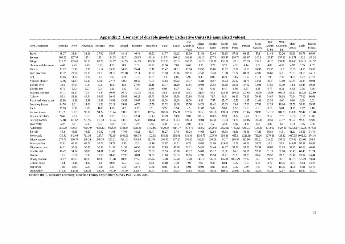
32

Appendix 2: User cost of durable goods by Federative Units (R$ annualized values)

Source: IBGE, Research Directory, Brazilian Family Expenditure Survey POF -2008-2009.

Item Description Rondônia Acre Amazonas Roraima Pará Amapá Tocantins Maranhão Piauí Ceará

Rio

Grande do

Norte

Minas

Gerais

Espírito

Santo

Rio de

Janeiro

São

PauloParaná

Santa

Catarina

Rio

Grande

do Sul

Mato

Grasso do

Sul

Mato

GrossoGoiás

Distrito

Federal

Stove 48.27 38.84 38.11 37.02 38.87 43.19 46.44 42.62 41.77 42.62 33.39 51.83 52.64 53.95 57.09 68.65 57.8 61.48 52.26 56.93 50.79 86.94

Freezer 108.25 127.58 127.4 127.4 134.33 132.71 156.63 264.6 117.74 200.16 161.98 138.45 127.3 283.47 150.78 128.07 140.1 127.17 157.83 142.71 140.3 146.24

Fridge 113.76 103.65 90.13 88.73 112.67 112.55 124.63 115.31 120.03 101.3 100.25 119.33 135.78 151.21 138.4 155.29 158.8 148.02 135.48 183.08 149.18 124.57

Shower with hot water 4.45 4.45 4.45 6.23 4.53 8.9 5.02 67.22 11.56 7,00 6.65 3.95 3.75 3.75 4.31 4.14 5.92 4.09 4.39 4.92 3.95 4.07

Blender 13.12 15.13 13.38 16.14 15.38 14.53 15.44 15.17 15.42 11.91 13.74 13.57 15.66 12.92 17.17 16.55 16.98 15.37 16.7 15.89 14.55 13.52

Food processor 41.37 21.06 29.19 29.19 29.19 226.68 32.14 32.27 35.18 39.16 108.09 27.47 33.28 23.58 12.74 80.01 42.09 16.61 24.81 20.93 24.65 24.17

Grill 11.05 14.02 12.87 9.1 8.97 9.01 8.54 8.57 13.1 6.06 5.95 9.49 8.07 8.29 14.5 11.92 11.14 7.03 7.38 11.85 8.77 21.78

Vacuum cleaner 52.96 54.83 55.37 55.93 27.78 124.7 60.49 70.01 30.04 98.12 54.77 35.83 38.57 28.63 29.82 38.78 44.61 38.6 57.89 57.89 48.35 59.04

Electric oven 41.6 47.54 41.6 41.6 41.6 41.6 27.06 21.18 11.77 21.18 11.91 30.04 25.56 28.68 23.51 47.92 43.91 37.56 41.39 74.4 53.44 19.38

Electric iron 6.71 5.92 5.27 6.04 6.26 6.32 7.41 6.99 6.99 6.27 6.2 7.23 6.49 6.41 8.56 8.81 8.28 6.77 8.24 8.52 7.05 7.36

Washing machine 43.71 82.37 70.04 45.44 50.94 36.79 141.35 54.63 52.2 135.28 99.51 131.34 89.9 133.33 160.25 103.65 148.96 118.86 105.08 58.87 162.29 202.69

Color tv 55.1 52.11 49.54 55.05 59.45 55.05 66.28 66.73 58.36 53.38 52.88 75.52 72.7 81.81 91.99 73.29 76.45 74.87 66.98 79.54 77.02 86.63

Black and white tv set 13.98 13.98 13.98 13.98 13.98 13.98 15.67 13.66 16,00 16,00 16,00 9.63 7.57 15.47 16.52 11.95 11.01 12.32 0,00 0,00 0,00 0,00

Sound equipment 14.74 9.31 14.08 11.28 22.11 35.01 46.78 15.58 20.32 19.88 15.58 24.23 19.42 40.03 19.4 17.06 17.92 21.24 16.86 27.56 33.38 19.95

Radio 15.93 6.38 8.49 10.8 4.38 4.2 7.75 3.71 5.76 2.94 4.5 11.07 9.49 9.68 8.51 11.63 6.83 9.15 5.84 11.45 9.87 9.18

Air conditioner 116.29 156.9 90.18 94.22 123.44 131.9 147.91 117.55 180.84 195.31 122.97 90.2 107.66 170.14 299.99 161.65 98.93 158.62 100.28 133.38 92.44 185.68

Fan /air circulator 9.41 7.83 8.57 11.21 9.79 7.83 12.34 10.43 11.29 9.03 9.03 10.16 10.02 9.98 11.32 9.73 9.55 9.17 7.77 10.87 9.32 11.85

Sewing machine 32.88 101.62 221.96 131.53 110.74 137.8 55.38 108.54 108.54 93.13 109.61 90.04 44.38 69.63 74.26 128.05 138.28 50.59 77.97 90.97 92.89 92.88

Water filter 3.27 4.81 2.56 6.07 4,00 6.94 5.88 3.45 3.42 3.15 2.03 3.67 5.2 3.58 4.56 14.16 20.1 8.87 6.6 5.74 3.45 6.06

Automobile 1215.28 1535.91 4615.49 4861.13 4958.35 6341.45 5786.36 3172.66 6720.26 4614.77 1874.75 4299.2 5432.65 3802.85 4730.62 5209.97 4726.11 3712.62 4720.45 4523.83 4152.76 5576.01

Bicycle 45.4 46.69 46.69 50.52 41.68 47.05 48.22 45.47 38.27 37.9 30.24 44.68 52.84 35.58 41.61 46.61 47.26 36.85 44.51 41.61 38.56 34.79

Motorcycle 430.42 942.64 731.36 267.7 742.65 1046.63 836.74 1102.02 856.36 692.01 631.46 1036.75 1025.84 658.33 655.9 1229.69 733.36 1270.83 426.82 1037.55 1045.92 274.18

Microcomputer 279.78 220.76 268.24 279.78 266.51 318.42 306.98 312.54 299.65 357.26 265.82 318.15 293.51 342.7 296.59 312.98 355.31 314.53 253.01 379.93 312.66 282.4

Water purifier 41.81 68.99 62.72 39.72 39.72 8.15 43.5 11.16 66.97 16.71 8.75 49.82 61.99 119.09 13.71 40.69 39.78 17.8 20.7 148.87 92.81 65.93

Microwave oven 44.21 55.61 53.35 36.33 51.32 51.32 46.99 65.36 53.63 45.78 51.21 54.31 52.44 44.37 51.58 53.28 52.34 48.89 52.63 54.27 62.69 40.45

Satellite dish 46.42 54.74 52,00 94.81 51.68 57.48 64.33 73.03 60.53 50.78 47.12 54.03 45.12 60,00 66.1 55.57 57.55 61.19 61.88 56.43 60.46 71.24

Dvd set 17.6 15.88 15.98 18.55 18.45 17.95 20.84 24.51 23.63 22.05 18.55 22.91 19.94 21.71 25.23 20.78 20.66 19.52 20.2 22.46 20.84 24.44

Drying machine 76.17 80.93 80.93 80.93 105.68 80.93 87.55 245.65 67.28 67.28 67.28 148.52 145.84 145.84 1007.79 77.32 77.9 88.78 98.51 80.59 375.21 93.64

Column mixer 11.4 11.18 14.82 9.3 10.96 12.3 9.32 12.4 10.08 7.38 7.99 9.5 9.48 8.04 10.32 11.59 9.98 8.72 10.55 14.93 8.13 14.27

Hair dryer 7.85 8.46 9.06 11.96 9.33 9.66 13.72 10.36 8.81 8.14 6.91 10.08 8.86 8.48 10.32 9.49 7.89 7.63 10.35 11.08 8.48 12.76

Dishwasher 178.39 178.39 178.39 178.39 178.39 178.39 200.87 35.64 35.64 35.64 35.64 105.58 189.66 189.66 203.02 207.85 192.85 190.96 82.87 82.87 82.87 83.1

33

Appendix 3 - Price Deflator by Geographical Context

Source: IBGE, Research Directory, Brazilian Family Expenditure Survey POF -2008-2009.

Appendix 4 - FGT class of poverty measures

Source: IBGE, Research Directory, Brazilian Family Expenditure Survey POF -2008-2009.

Geographical Context Price Deflator

Metropolitan urban area of Belém 0.93

Urban North excluding metropolitan urban areas 0.94

Rural North 0.89

Metropolitan urban area of Fortaleza 0.90

Metropolitan urban area of Recife 0.89

Metropolitan urban area of Salvador 0.98

Urban Northeast excluding metropolitan urban areas 0.90

Rural Northeast 0.86

Metropolitan urban area of Belo Horizonte 1.03

Metropolitan urban area of Rio de Janeiro 0.96

Metropolitan urban area of São Paulo 1.00

Urban Southeast excluding metropolitan urban areas 0.96

Rural Southeast 0.92

Metropolitan urban area of Curitiba 0.95

Metropolitan urban area of Porto Alegre 1.00

Urban South excluding metropolitan urban areas 0.95

Rural South 0.82

Brasília (FD) 1.02

Urban Midwest excluding Brasília 1.01

Rural Midwest excluding Brasília 0.95

FGT(0) FGT(1) FGT(2) FGT(0) FGT(1) FGT(2)

0.1460 0.0456 0.0206 0.0528 0.0147 0.0063

(0.0078) (0.0032) (0.0018) (0.0046) (0.0017) (0.0010)

0.1900 0.0628 0.0291 0.0781 0.0216 0.0089

(0.0042) (0.0017) (0.0009) (0.0027) (0.0009) (0.0004)

0.4053 0.1612 0.0843 0.2209 0.0709 0.0321

(0.0093) (0.0050) (0.0033) (0.0079) (0.0034) (0.0020)

0.3144 0.1095 0.0516 0.1436 0.0390 0.0157

(0.0111) (0.0052) (0.0030) (0.0085) (0.0029) (0.0014)

0.3841 0.1454 0.0738 0.1922 0.0602 0.0269

(0.0066) (0.0034) (0.0022) (0.0055) (0.0023) (0.0013)

0.1249 0.0386 0.0176 0.0447 0.0128 0.0055

(0.0063) (0.0025) (0.0014) (0.0035) (0.0014) (0.0008)

0.0941 0.0269 0.0111 0.0309 0.0069 0.0026

(0.0064) (0.0022) (0.0011) (0.0035) (0.0009) (0.0004)

0.1877 0.0607 0.0272 0.0790 0.0190 0.0071

(0.0094) (0.0038) (0.0020) (0.0068) (0.0017) (0.0007)

0.2133 0.0743 0.0359 0.0947 0.0279 0.0121

(0.0037) (0.0016) (0.0009) (0.0024) (0.0009) (0.0005)

Southeast

South

Midwest

Brazil

Poverty Line = R$185

Metropolitan

Geographic Areas

and Major Regions

Poverty Line = R$117

Urban

Rural

North

Northeast

34

Appendix 5 – Explanatory variables and estimated coefficients (α) of the

heterocedastic model

Source: IBGE, Research Directory, Brazilian Family Expenditure Survey POF -2008-2009.

Appendix 6 – Explanatory variables and estimated coefficients (β)

Source: IBGE, Research Directory, Brazilian Family Expenditure Survey POF -2008-200

Variable Coefficient Standard Error t Value Pr > |t|

Intercept -4.1457 0.1162 -35.66 <.0001

If the household is own -0.0957 0.0222 -4.32 <.0001

If the household head has 7 years and less of school completed 0.1014 0.0229 4.43 <.0001

If the household has lighting provided by the supply company -0.2671 0.0622 -4.30 <.0001

Indirectly collected garbage -0.0955 0.0390 -2.45 0,014

If the household is in the urban area -0.3067 0.0331 -9.28 <.0001

If the household has sewage system -0.1072 0.0241 -4.45 <.0001

If the hous ehold is in the metropolitan urban area of Belém -0.4224 0.1009 -4.19 <.0001

If the household is in the rural North -0.2331 0.0601 -3.88 0.0001

If the household is in the rural Northeast -0.2249 0.0494 -4.55 <.0001

If the household is in the urban Southeast, excluding metropolitan

urban areas 0.1349 0.0303 4.46 <.0001

If the household is in the metropolitan urban area of Curitiba 0.4406 0.1089 4.05 <.0001

If the household head is an employee -0.0742 0.0206 -3.61 0,000

If the household head has never studied 0.0745 0.0299 2.49 0,013

Members of household per room 0.1510 0.0266 5.68 <.0001

Proportion of household members receiving some income -0.1571 0.0489 -3.21 0,001

Logarithm of per capita disposable monetary income -0.1330 0.0168 -7.93 <.0001

Interaction between the logarithm of the household income and the

logarithm of the ratio between the per capita disposable monetary

income of the household and the median of geographical context

0.0025 0.0007 3.8 0,0001

Logarithm of the total of household members, excluding private

household workers and household lodgers -0.2642 0.0266 -9.95 <.0001

Logarithm of the ratio between the per capita disposable monetary

income of the household and the median of geographical context 0.1998 0.0431 4.64 <.0001

Proportion of people in municipality receiving Bolsa Família in 2010 1.1757 0.2687 4.38 <.0001

R2

Observações

0,016

56091

Variables CoefficientsStandard

Errort Value Pr > |t|

Intercept 4.2882 0.3752 11.4294 <0,0001

If the household is in the metropolitan urban area of Belém 0.0658 0.0289 2.2818 0,0113

If the household is in the urban North, excluding metropolitan urban areas 0.0559 0.0141 39.722 <0,0001

If the household is in the rural North 0.1614 0.0238 6.7944 <0,0001

If the household is in the metropolitan urban area of Fortaleza -0.1294 0.0317 -4.0877 <0,0001

If the household is in the metropolitan urban area of Recife -0.0941 0.0243 -3.8717 <0,0001

If the household is in the metropolitan urban area of Salvador -0.0493 0.0274 -1.7955 0,0363

If the household is in the rural Northeast 0.0484 0.0186 2.6067 0,0046

If the household is in the metropolitan urban area of Belo Horizonte -0.0818 0.0225 -3.6408 0,0001

If the household is in the metropolitan urban area of Rio de Janeiro -0.0391 0.0222 -1.7570 0,0395

If the household is in the rural Southeast 0.0437 0.0222 1.9643 0,0248

If the household is in the metropolitan urban area of Curitiba -0.1192 0.0369 -3.2278 0,0006

If the household is in the metropolitan urban area of Porto Alegre 0.0804 0.0268 2.9929 0,0014

If the household is in the urban South, excluding metropolitan urban areas 0.0589 0.0142 4.1403 <0,0001

If the household is in the rural South 0.2316 0.0274 8.4649 <0,0001

If the household is in the urban Midwest, excluding Distrito Federal -0.0954 0.0133 -7.1780 <0,0001

If the household has piped water in at least one room 0.0878 0.0129 6.8144 <0,0001

If the household head holds health plan 0.0860 0.0083 10.3294 <0,0001

If the household head has 7 years and less of school completed -0.0690 0.0089 -7.7306 <0,0001

If the street where the household is located has paving 0.0641 0.0078 8.1753 <0,0001

Literate household head 0.1357 0.0090 15.0436 <0,0001

If the household is rented -0.1330 0.0084 -15.8477 <0,0001

If the household head is white 0.0606 0.0064 9.4147 <0,0001

Householder attendence: public school, college 0.1121 0.0207 5.4205 <0,0001

No bathroom in the household -0.3442 0.0226 -15.2026 <0,0001

One bathroom in the household -0.2962 0.0140 -21.1622 <0,0001

Two bathrooms in the household -0.1097 0.0135 -8.0955 <0,0001

Uncoated mud with wall household -0.1441 0.0233 -6.1791 <0,0001

Type of family: husband-wife household having children 0.0648 0.0074 8.7874 <0,0001

If the household head has 11 to 14 years of school completed 0.0493 0.0097 5.1054 <0,0001

If the household head has 15 years and over of school completed 0.1730 0.0142 12.2039 <0,0001

If the household head is an employer 0.2321 0.0160 14.5092 <0,0001

If the household head is an own account 0.0788 0.0069 11.3453 <0,0001

Members of household per room -0.2359 0.0107 -22.0954 <0,0001

If the household is in the last decile of the the per capita disposable monetary income distribution-0.0581 0.0141 -4.1074 <0,0001

Logarithm of the total of adult members in the household 0.1432 0.0176 8.1156 <0,0001

Logarithm of the household head age 0.3786 0.1948 1.9436 0,0260

Squared logarithm of the household head age -0.0467 0.0265 -1.7630 0,0389

Logarithm of the total of elderly members in the household -0.0898 0.0126 -7.1137 <0,0001

Logarithm of the total of household members, excluding private household workers and household lodgers -0.4000 0.0140 -28.5074 <0,0001

Logarithm of per capita disposable monetary income -0.0476 0.0206 -2.3128 0,0104

Squared logarithm of per capita disposable monetary income 0.0349 0.0019 17.8972 <0,0001

Logarithm of the ratio between the per capita disposable monetary income of the household and the median of geographical context-0.0183 0.0175 -1.0414 0,1489

Logarithm of gross domestic product per capita 0.0409 0.0099 4.1526 <0,0001

Total of children under 7 years old in the household -0.0275 0.0056 -4.9012 <0,0001

Proportion of people in municipality receiving Bolsa Família in 2010 -11622 0.1728 -6.7239 <0,0001

Proportion of people with complete college in the enumeration area 0.2088 0.0272 7.6626 <0,0001

Proportion of household head who holds health plan in the enumeration area 0.1881 0.0337 5.5777 <0,0001

R2

Observations

0.75

56091

35

Appendix 7 – Estimated proportion of people vulnerable to poverty versus the estimated proportions of the poor calculated directly from POF by the 20 geographical contexts which

take part in Geographical Areas and Major Regions (Poverty line = R$185)

Source: IBGE, Research Directory, Brazilian Family Expenditure Survey POF -2008-2009.

VI >= 0.5 0.2 <VI < 0.5 VI >= 0.5 0.2 <VI < 0.5

Metropolitan urban area of Belém 0.1766 0.1677 0.1414 0.6161 0.2108

Urban North excluding metropolitan urban

areas0.2647 0.2501 0.1911 0.6326 0.2502

Rural North 0.4852 0.4854 0.2259 0.7606 0.1831

Metropolitan urban area of Fortaleza 0.2997 0.2853 0.2396 0.6537 0.2668

Metropolitan urban area of Recife 0.2911 0.1947 0.2271 0.5291 0.3026

Metropolitan urban area of Salvador 0.2765 0.1827 0.1947 0.5535 0.3174

Urban Northeast excluding metropolitan

urban areas0.3326 0.2802 0.2331 0.6443 0.2592

Rural Northeast 0.5479 0.5697 0.2612 0.7917 0.1742

Metropolitan urban area of Belo Horizonte 0.1131 0.0637 0.1205 0.3831 0.3879

Metropolitan urban area of Rio de Janeiro 0.1341 0.0569 0.1218 0.3079 0.4545

Metropolitan urban area of São Paulo 0.0986 0.067 0.1018 0.5116 0.3106

Urban Southeast excluding metropolitan

urban areas0.1119 0.0622 0.1011 0.4279 0.3413

Rural Southeast 0.2595 0.1689 0.2405 0.4579 0.3600

Metropolitan urban area of Curitiba 0.0968 0.0851 0.1081 0.4579 0.3448

Metropolitan urban area of Porto Alegre 0.0917 0.0331 0.1008 0.2909 0.4374

Urban South excluding metropolitan urban

areas0.0874 0.0392 0.0877 0.3171 0.369

Rural South 0.1192 0.0355 0.1152 0.2291 0.4371

Distrito Federal 0.1172 0.0769 0.1060 0.4714 0.2693

Urban Midwest excluding Distrito Federal 0.1918 0.1276 0.1693 0.4799 0.3300

Rural Midwest excluding Distrito Federal 0.2760 0.1962 0.2668 0.4828 0.3588

Brazil 0.2133 0.1680 0.1584 0.5891 0.2772

Geographical contextPoverty

incidence POF

Vulnerability incidence

(VI)

Vulnerability incidence of

poor people (VI)

36

Appendix 8 – Per Capita Consumption Aggregate versus Total Per Capita Expense and Per Capita General Consumption Expenditure calculated by POF – Brazil

(a) Density Curves

Source: Brazilian Family Expenditure Survey POF -2008-2009, IBGE.

(b) Poverty Curves

Source: Brazilian Family Expenditure Survey POF -2008-2009, IBGE.

(c) Lorenz Curves

Source: Brazilian Family Expenditure Survey POF -2008-2009, IBGE.

0

.05

.1

.15

.2

.25

.3

.35

.4

.45

1 2 3 4 5 6 7 8 9 10

ln(Per Capita Consumption Agregate) ln(Per Capita Total Expenditure from POF)

ln(Per Capita General Consumption Expenditure from POF)

0

.002

.004

.006

.008

.01

.012

.014

0 20 40 60 80 100 120

Poverty line (z)

Per Capita Consumption Agregate Total Expenditure from POF

Per Capita General Consumption Expenditure

0

.1

.2

.3

.4

.5

.6

.7

.8

.9

1

0 .1 .2 .3 .4 .5 .6 .7 .8 .9 1Percentiles (p)

45° line Per Capita Consumption Agregate

Total Expenditure from POFPer Capita General Consumption Expenditure

37

(d) Mean Estimates, Coefficient of Variation, FGT (alfa=2), Gini Index and Probabilities

Source: Brazilian Family Expenditure Survey 2008-2009, IBGE.

Where:

X1 = Total Expenditure = all the monetary and non-monetary expenses registered by POF.

X2 = Consumption Expenditure = total expenditure - patrimonial variation – (taxes + labor deductions + bank services + pensions+ allowances+ donations+ private social security)

X3 = Consumption Aggregate = aggregate built in section 1.

ESTIMATES

X1= Per Capita

Total Expenditure

from POF

X2= Per Capita

Consumption Expenditure

from POF

X3= Per Capita

Consumption AgregateX3-X1 X3-X2

MEAN(X) 799 649 621 -178 -28

Std. Err. 12,569 9,000 8,117 5,722 2,158

P-value 0,000 0,000 0,000 0,000 0,000

CV(X) 1,625 1,336 1,216 -0,408 -0,120

Std. Err. 0,044 0,028 0,023 0,038 0,014

P-value 0,000 0,000 0,000 0,000 0,000

FGT(X, Z=117, alfa=2)x100 1,184 1,337 1,205 0,021 -0,132

Std. Err. 0,001 0,059 0,051 0,028 0,029

P-value 0,000 0,000 0,000 0,447 0,000

FGT(X, Z=185, alfa=2)x100 3,232 3,662 3,592 0,360 -0,070

Std. Err. 0,095 0,099 0,095 0,041 0,040

P-value 0,000 0,000 0,000 0,000 0,080

GINI(X) 0,554 0,516 0,501 -0,053 -0,015

Std. Err. 0,004 0,004 0,004 0,002 0,001

P-value 0,000 0,000 0,000 0,000 0,000

Prob(X ≤ 80) 0,037 0,043 0,040 0,003 -0,002

Std. Err. 0,002 0,002 0,002 0,001 0,001

P-value 0,000 0,000 0,000 0,002 0,011

Prob(X ≤ 120) 0,086 0,098 0,099 0,013 0,002

Std. Err. 0,002 0,002 0,002 0,001 0,001

P-value 0,000 0,000 0,000 0,000 0,207

Prob(X ≤ 400) 0,461 0,511 0,514 0,053 0,003

Std. Err. 0,005 0,005 0,005 0,002 0,002

P-value 0,000 0,000 0,000 0,000 0,146

Prob(X ≤ 2000) 0,922 0,949 0,956 0,034 0,007

Std. Err. 0,003 0,002 0,002 0,002 0,001

P-value 0,000 0,000 0,000 0,000 0,000

Prob(X ≤ 4000) 0,978 0,988 0,992 0,014 0,004

Std. Err. 0,001 0,001 0,001 0,001 0,000

P-value 0,000 0,000 0,000 0,000 0,000