construction of a database for the biogeochemical...
TRANSCRIPT

Construction of a database for the biogeochemical classification of estuaries
© Deltares, 2011
Veronica Minaya Claudette Spiteri


22 September 2011, final
Construction of a database for the biogeochemical classification of estuaries
i
Contents
1 Introduction 3 1.1 Estuarine physical features 3
1.1.1 Geometry 3 1.1.2 Hydrodynamics 4
1.2 Estuarine biogeochemical features 5 1.2.1 Biogeochemical substances 6 1.2.2 Nutrient Fluxes 7
1.3 Existing estuarine classifications and databases 9
2 Aim 10
3 Methodology 11 3.1 Construction of database 11 3.2 Calculation of the width convergence length (b) of estuaries 12 3.3 Statistical Analyses 17
4 Results and Discussion 17 4.1 Distribution of estuaries in the database 17 4.2 Hydrodynamic parameters 19
4.2.1 Variation with latitude 19 4.2.2 Variation with estuarine shape/width convergence length 22
4.3 Biogeochemical behavior 25 4.3.1 Nutrient concentrations 25 4.3.2 Carbon concentrations 35 4.3.3 Total Suspended Solids (TSS) 39
5 Shortcomings 41 5.1 Physical and geometrical parameters 41 5.2 Biogeochemical parameters 42
6 Summary and outlook 42
7 References 45
ANNEX A 54
ANNEX B 58
ANNEX C 60
ANNEX D 62
ANNEX E 67

22 September 2011, final
Construction of a database for the biogeochemical classification of estuaries
3
Construction of a dataset for the biogeochemical classification of estuaries
1 Introduction
Estuaries are land-ocean transition zones where rivers meet the sea. An estuary can be either the discharge of freshwater from the river into the coastal zone or the fill of salty water from the sea in the estuary (Savenije, 2005). The high importance of estuaries is that they provide a unique aquatic environment that hosts a broad biodiversity from two different water bodies. Having specific hydraulic, morphologic and biologic characteristics, estuaries serve as an ecotone between two adjacent communities, containing species characteristic of both, as well as other species specific to this zone. Therefore, they play an important role not only for the life cycle of flora and fauna species but also for the goods and services that they can provide to humankind (Savenije, 2005). Due to the potential features of estuaries, most of the population growth has been taking place in coastal areas close to estuaries. As a consequence, estuaries have been under constant pressure caused by, for example, the increase of nutrient inputs leading to the deterioration of ecological health. Apart from the role of estuaries in the delivery of land-derived nutrients to the coastal zone, their importance in the CO2 air-water exchange fluxes and hence in the global carbon cycle has recently been advocated (Borges, 2005) The functioning of estuaries is controlled by the complex combination of hydrodynamic, geological, geochemical and biological processes that are interlinked and that act at different time and spatial scales.
1.1 Estuarine physical features
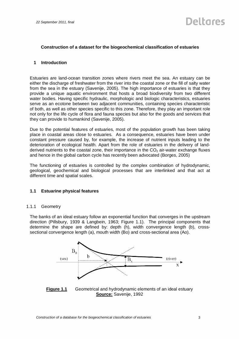
1.1.1 Geometry The banks of an ideal estuary follow an exponential function that converges in the upstream direction (Pillsbury, 1939 & Langbein, 1963; Figure 1.1). The principal components that determine the shape are defined by: depth (h), width convergence length (b), cross-sectional convergence length (a), mouth width (Bo) and cross-sectional area (Ao).
Figure 1.1 Geometrical and hydrodynamic elements of an ideal estuary Source: Savenije, 1992

4
22 September 2011, final
Construction of a database for the biogeochemical classification of estuaries
expoxB Bb [Eq 1]
The width convergence length (b), defined as the distance measured from the mouth to the point where the tangents intersect the x axis, is an indicator of estuarine shape and it is directly related to the dominant hydrodynamic regime. Estuarine geometries vary between funnel-shaped, characterized with low values of b and converging upstream banks, and prismatic, having a relatively high b, parallel banks and a constant cross-section (Figure 1.2). According to Savenije (1992), the shape of the estuary is influenced by a combination of factors, including tidal movement, river floods, wave and storm action.
Figure 1.2 Estuarine shape classification based on the width convergence length
1.1.2 Hydrodynamics The hydrodynamic ratio, also known as the Canter-Cremers number (C), gives information on the hydrodynamic characteristics of an estuary and is calculated as shown in Equation 2. The non-dimensional estuarine shape number (S) is determined by Equation 3. Based on an analysis of 18 estuaries (Savenije, 2006), a relationship was established between C and S, as indicated in Equation 4.
bQ TCP
[Eq 2]
aSH
[Eq 3]
Where: C: Canter-Cremers number Qb: bankfull discharge T: tidal period P: tidal prism S: estuarine shape number a: cross-sectional convergence length H: mean water depth
0.2612500( )S C [Eq 4]
b low b high

22 September 2011, final
Construction of a database for the biogeochemical classification of estuaries
5
Due to the interdependence between the geometrical, hydrodynamical and biogeochemical functioning of estuaries (Figure 1.3), the combination of C and S gives insight in the biogeochemical behavior as shown in Arndt (2008).
Figure 1.3 Physical forcing components and the interaction with estuarine
biogeochemistry Source: Arndt, 2008
1.2 Estuarine biogeochemical features As a result of the population increase, anthropogenic activities on land such as food production, land use conversion, sewage discharges, and the construction of dams for hydropower, have among others, modified the hydrological regimes and the export of dissolved and particulate nutrients from land to rivers and finally to the coastal seas (Meybeck & Vorosmarty, 2005; Seitzinger et al., 2010). The increase in nutrient levels has brought positive and negative consequences. On one hand, it has allowed food production coping with the population growth demands but on the other hand, it has modified the ecosystems due to the increase in nutrient export to the coast leading to possible eutrophication risks and other environmental impacts.
6
22 September 2011, final
Construction of a database for the biogeochemical classification of estuaries
1.2.1 Biogeochemical substances Silica
Dissolved silica is one of the most important elements in the marine and continental systems, while particulate silica plays an important role in the nutrient cycle of surface estuaries. Both dissolved and particulate silica are derived from the weathering processes of sedimentary rocks. Dissolved silica concentrations are also being modified due to the increase in nitrogen and phosphorus related to human activities and the long residence times in reservoirs behind dams. According to Eyre and Balls (1999), estuaries located in the tropical estuaries have much higher silicate concentrations in comparison to temperate estuaries. The largest contributors of SiO2 are South America (25%) and Asia (23%) (Bouwman et al., 2010).
Nitrogen
Nitrogen is transported is various forms such as nitrate (NO3-), nitrite (NO2
-), and ammonium (NH4
+), collectively known as dissolved inorganic nitrogen (DIN), dissolved organic nitrogen (DON), and particulate nitrogen (PN). Most of the nitrogen concentration associated with anthropogenic activities, such as excess fertilization and animal waste in agricultural lands, is transported to rivers through runoff. Sewage and atmospheric deposition of NH4
+ from industries also contribute to the DIN pool (Bouwman et al., 2010). The changes in agriculture and land use have increased the levels of DIN in rivers by approximately 30%. Consequently, an increase in the export fluxes to coastal waters has also been observed, in particular in South Asia where more than half of the global increase has occurred (Seitzinger et al., 2010). A small percentage of nitrogen comes from non-anthropogenic sources, including organic matter degradation and internal recycling in sediments.
Phosphorus In aquatic systems, phosphorus occurs as dissolved inorganic phosphorus (DIP), dissolved organic phosphorus (DOP), particulate inorganic phosphorus (PIP) and particulate organic phosphorus (POP). As for nitrogen, phosphorus is associated to anthropogenic activities and is transported to the coastal systems through estuarine pathways, although a significant fraction of DIP is generally retained in estuaries due to sorption. According to Seitzinger et al. (2010), the main sources that contribute to the rising levels of DIP are sewage effluent and detergent use rather than agriculture.
Carbon
Every year 0.9 Gt of carbon is transported by rivers in the world, of which 40% is organic and 60% inorganic (Meybeck, 1993). Carbon fluxes are likely to increase due to anthropogenic activities (Abril et al., 2002). Dissolved organic carbon (DOC) goes through strong changes in nature and composition in estuaries (Abril et al., 2002). Particulate organic carbon (POC) is generated by the dynamics of suspended sediments and is therefore extremely heterogeneous. It is subject to sedimentation and erosion during neap and spring tides, part of which deposits in estuaries while the rest is exported to the coastal zones (Abril et al., 1999). Polluted rivers and estuaries tend to have higher concentrations of POC.
22 September 2011, final
Construction of a database for the biogeochemical classification of estuaries
7
Total Suspended Solids
Total suspended solids (TSS) are key elements for the uptake and release of chemical components in the water column. Dissolved and suspended particulate in water are related to conductance and turbidity (light availability in estuaries) therefore have important implications on the ecological processes, such as primary production. TSS are related to the weathering rates, erosion and discharges rates. TSS also absorb heat and increase surface water temperature playing an important role in surface estuaries (Mitchell and Stapp, 1992).
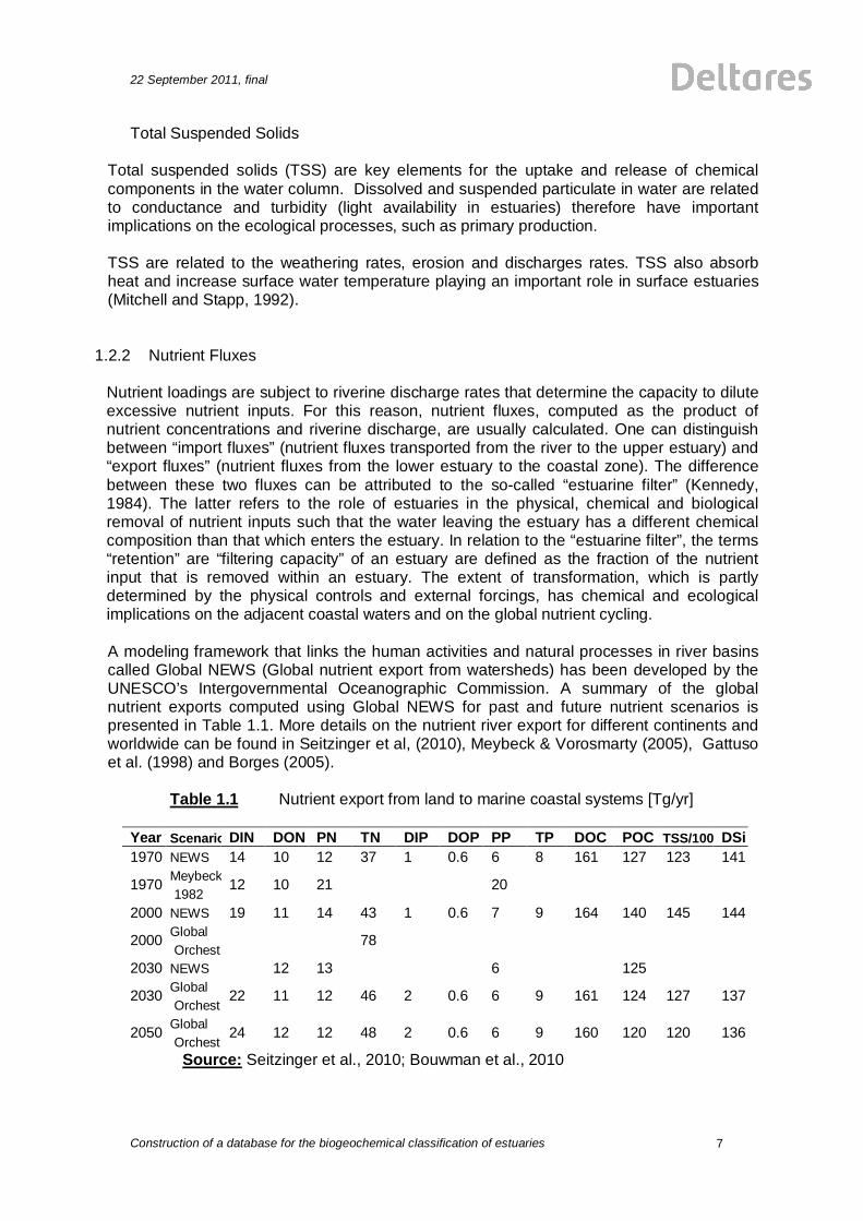
1.2.2 Nutrient Fluxes Nutrient loadings are subject to riverine discharge rates that determine the capacity to dilute excessive nutrient inputs. For this reason, nutrient fluxes, computed as the product of nutrient concentrations and riverine discharge, are usually calculated. One can distinguish between “import fluxes” (nutrient fluxes transported from the river to the upper estuary) and “export fluxes” (nutrient fluxes from the lower estuary to the coastal zone). The difference between these two fluxes can be attributed to the so-called “estuarine filter” (Kennedy, 1984). The latter refers to the role of estuaries in the physical, chemical and biological removal of nutrient inputs such that the water leaving the estuary has a different chemical composition than that which enters the estuary. In relation to the “estuarine filter”, the terms “retention” are “filtering capacity” of an estuary are defined as the fraction of the nutrient input that is removed within an estuary. The extent of transformation, which is partly determined by the physical controls and external forcings, has chemical and ecological implications on the adjacent coastal waters and on the global nutrient cycling. A modeling framework that links the human activities and natural processes in river basins called Global NEWS (Global nutrient export from watersheds) has been developed by the UNESCO’s Intergovernmental Oceanographic Commission. A summary of the global nutrient exports computed using Global NEWS for past and future nutrient scenarios is presented in Table 1.1. More details on the nutrient river export for different continents and worldwide can be found in Seitzinger et al, (2010), Meybeck & Vorosmarty (2005), Gattuso et al. (1998) and Borges (2005).
Table 1.1 Nutrient export from land to marine coastal systems [Tg/yr]
Year Scenario DIN DON PN TN DIP DOP PP TP DOC POC TSS/100 DSi 1970 NEWS 14 10 12 37 1 0.6 6 8 161 127 123 141
1970 Meybeck, 1982
12 10 21 20
2000 NEWS 19 11 14 43 1 0.6 7 9 164 140 145 144
2000 Global Orchest.
78
2030 NEWS 12 13 6 125
2030 Global Orchest
22 11 12 46 2 0.6 6 9 161 124 127 137
2050 Global Orchest
24 12 12 48 2 0.6 6 9 160 120 120 136
Source: Seitzinger et al., 2010; Bouwman et al., 2010

8
22 September 2011, final
Construction of a database for the biogeochemical classification of estuaries
The transition of the nutrient exports from 1970 to 2000 and the future trends based on different scenarios are shown in the Figure 1.4.
Figure 1.4 Transition of nutrient export between 1970 and 2000 and future scenarios
between 2000 and 2030 (NEWS Results) Source: Seitzinger et al., 2010
In the context of climate change, more attention has been recently given to link between nutrient and CO2 fluxes in the coastal ocean since they act as sinks for organic matter and therefore potential sources of CO2 to the atmosphere (Gattuso et al., 1998; Borges, 2005). An impact on the land-ocean interaction due to the global change is also envisaged, as shown by Holmes et al. (2000) in an analysis of nutrient fluxes from Russian rivers to the Arctic Ocean. For this reason, the understanding of current nutrient behavior and fluxes will help constrain the models used for predicting future changes in nutrient fluxes and their ecological implications.

22 September 2011, final
Construction of a database for the biogeochemical classification of estuaries
9
1.3 Existing estuarine classifications and databases
In order to understand the global functioning of estuaries it is crucial to identify and group estuaries with similar characteristics. This is the basis of traditional estuarine classifications that are generally based on physical parameters, such as geometrical/geomorphic features (Pritchard 1955, 1967), hydrodynamic behaviour and mixing patterns (Cameron and Pritchard, 1963). Classical geomorphological classifications consider four subdivisions (Dalrymple et al., 1992): 1) drowned river valleys, 2) fjord type estuaries, 3) bar-built estuaries and 4) estuaries produced by tectonic processes (Pritchard, 1967). The classifications proposed by Hume and Herdendorf (1988) are based on the origin and behavioral features of estuaries. Other classification criteria are based on the presence of a single or multiple mouth, constructed or unconstructed mouth, branched or unbranched main drainage lines, giving rise to 32 possible combinations of physical types (Pierson et al., 2002). Pethick (1984) proposed a classification of estuaries based on three groups according to their tidal range: micro-tidal estuaries (range < 2m), meso-tidal estuaries (range between 2 to 4m) and macro-tidal (range > 4m). However, such a classification has limited relevance to studies of estuarine morphology (Savenije, 1992). For instance, although Banyuasin and Lalang estuaries both have the same tidal range, their shape and morphology varies significantly. With a convergence length of 20 km, Banyuasin is funnel-shaped whereas Lalang has a convergence length of 200km and is therefore prismatic-shaped (Savenije, 1992). This implies that depending on the attributes used for defining the categories, different estuarine classifications may lead to equivocal groups. Also, it is important to note that real estuaries do not always fall within the idealized classification categories. Even though the classifications based on geometry and hydrodynamics features may appear to be unrelated, they are in fact directly correlated. This was illustrated by Savenije (2005) in his classification based on shape, tidal influence, river influence, geology and salinity. In the latter, the width convergence length (b), defined as the distance from the mouth to the point where the tangents intersect the x axis (Savenije, 2002), was used as the main classification indicator. More recent classification schemes (e.g. Hume et al., 2007; Swaney et al. 2008; Arndt, 2008) generally aim at increasing the understanding and ability to predict the response of coastal ecosystems to enhanced nutrient delivery. For example, Swaney et al. (2008) proposed a simple estuarine classification scheme focusing on the biological response of the river-dominated estuarine systems and the role of water residence time using nutrient-phytoplankton-zooplankton models. The ‘estuary environment classification’ presented in Hume et al. (2007) considers a four-level hierarchical system of the abiotic components, such as climatic, oceanic, riverine and catchment factors, that determine the physical and ecological characteristics of estuaries. Arndt (2008) proposes an estuarine classification based on the mutual interdependence between: 1) geometry and hydrodynamics, and 2) hydrodynamics and biogeochemistry (Figure 1.3). Here a reactive transport modelling approach is proposed that accounts explicitly for the coupling of hydrodynamics and biogeochemistry along the tidal river-coastal sea continuum, including the mechanistic process-based description of the estuarine filter. Studies of estuarine functioning at the global-scale rely on databases in which site-specific geometric, hydrodynamic or biogeochemical data of estuaries are collected. Extensive literature review has revealed that various estuarine databases are already available.

10
22 September 2011, final
Construction of a database for the biogeochemical classification of estuaries
However, in all cases, these databases focus either on one particular country or on one set of attributes, mainly hydrodynamic or ecological features. Toffolon and Savenije (2008) have put together an inventory of databases of estuaries worldwide, called DBest, focusing on morphology and hydrodynamic features. A list of country-based estuarine databases considered by Toffolon and Savenije (2008) is given below:
Australia and New Zealand: • Australian Estuarine Database - AED • Australian Estuaries Database - CAMRIS • OZCoast and OzEstuaries - Australia's online coastal information portal • Simple Estuarine Response Model (SERM I and SERM II, Australia): datasets • Australia - Coastal Habitat Resources Information System (CHRIS) • New Zealand - Estuaries database UK: • British Oceanographic Data Centre - Estuaries Database 2003 • The Estuary Guide - Estuaries database USA: • National Estuarine Eutrophication Assessment - NEEA Estuaries Database • USGS-South Florida Information Access (SOFIA) - Ecosystem History of South Florida Estuaries Data • NOAA's Estuary Restoration Act (ERA) - National Estuaries Restoration Inventory • Henry Lee's estuarine database seems more concerned with ecological problems. In another study carried out by WL| Delft Hydraulics, a geomorphological database for European estuaries was constructed and used as the basis for the development of a “Generic Estuary Model for Contaminants” (GEMCO, 2003).
2 Aim
Within the large scale project on “The quantitative significance of estuaries for the CO2 pumping efficiency of the global coastal ocean“, three main objectives are identified (Figure 2.1): 1. To compile a global database for estuaries through extensive literature search that
includes geometric, hydrodynamic and biogeochemical features 2. To set up estuarine hydrodynamic-biogeochemical modeling scenarios based on the
data collected in the database 3. To assess the contribution of estuaries to CO2 air/water fluxes at the local scale and
extrapolate to global scale This report focuses on the first objective, i.e. the construction of the global estuarine geometrical, hydrodynamical and biogeochemical database. Since it is not possible to study all estuaries world-wide, the aim of this database is to identify and group estuaries with similar characteristics and use this information to define estuarine model scenarios, to be used in the step 2 of the project (outside scope of this study).

22 September 2011, final
Construction of a database for the biogeochemical classification of estuaries
11
Figure 2.1 Scheme for the main objectives of the project Source: Modified from Savenije (2005)
3 Methodology
3.1 Construction of database
Table 3.1 summarizes the main estuarine attributes compiled in the database. Data was organized in two main excel sheets; one with physical attributes, one with biogeochemical parameters.
Table 3.1 Main attributes included in the estuarine database
Physical Biogeochemical Climate:
Latitude Longitude Temperature (ToC) Incident solar radiation
Nutrient concentrations [mg/l]: Silica: Si Nitrogen: NO3
- NO2 NH4
+ DIN DON PN
Phosphorus: DIP DOP PP
Hydrodynamic: Discharge (Q) [m3/s] Basin area (A) [km2] Runoff [mm/yr]
Carbon concentrations [mg/l]: DIC DOC POC HCO3
- Total Alkalinity pH pCO2 CH4
TN
TOC

12
22 September 2011, final
Construction of a database for the biogeochemical classification of estuaries
Physical Biogeochemical Geometric:
Water depth at the mouth (ho) Mouth area (Ao) Width at the mouth (Bo) Tidal range at the mouth (Ho) Cross-sectional convergence length (a) Width convergence length (b)
Others: Total suspended solids (TSS) Salinity intrusion length (Ls)
Note:
DIN Dissolved Inorganic Nitrogen DON Dissolved Organic Nitrogen TN Total Nitrogen PN Particulate Nitrogen DIP Dissolved Inorganic Phosphorus DOP Dissolved Organic Phosphorus PP Particulate Phosphorus DIC Dissolved Inorganic Carbon DOC Dissolved Organic Carbon POC Particulate Organic Carbon TOC Total Organic Carbon
All the data entries were collected from primary sources, including scientific papers, publicly-available databases and other information (refer to Annex A for a list of links to estuarine studies and data) with the exception of the width convergence length (b). This parameter is not readily available in literature and therefore was calculated as explained below. For hydrodynamic parameters, such as discharge rates, annual average values were considered whereas for the chemical parameters, average concentrations at salinity zero or close to zero were considered whenever available.
3.2 Calculation of the width convergence length (b) of estuaries Based on the work Savenije (1992), the following methodology for the calculation of the width convergence length (b) was established. Although the methodology is similar to that used in previous studies, for example (Bals, 2002), satellite images were used here for measuring geometrical features instead of site maps. In accordance to the relation between B and x (Eq 1), the following steps were taken:
1) Width at the mouth [Bo]
Google Earth (imagery date between 2005 and 2010) was used to measure the width at the mouth of a specific estuary.
2) Width [B(x)] at different distances [x]
The width and distances were measured upstream in each change of direction of the river. Multiple measurements were taken to obtain high resolution of the estuarine profile (Figure 3.1).

22 September 2011, final
Construction of a database for the biogeochemical classification of estuaries
13
Figure 3.1 Measurement of the estuarine width at the mouth and at different x (Barito Estuary)
Source: Google Earth, imagery July 2005
In cases where islands were found in the middle of the channel, only the width of the active channel was considered [Figure 3.2].
Bo [km]
x
B(x)

14
22 September 2011, final
Construction of a database for the biogeochemical classification of estuaries
Figure 3.2 Measurement of the width in case of isles within the channel Source: Google Earth, imagery July 2005
3) The measurements taken (x and B(x)) were plotted. From the graph, the
inflection point was determined [Figure 3.3].
Distance vs w idth
0
2
4
6
8
10
12
14
16
0 10 20 30 40 50 60
Distance (km)
Wid
th (k
m)
Figure 3.3 Determination of inflection point
4) x and log B(x) were plotted in order to derive the equation of the trend line for the points before the inflection point [Figure 3.4].
Inflection point
Weser Estuary

22 September 2011, final
Construction of a database for the biogeochemical classification of estuaries
15
0
0.2
0.4
0.6
0.8
1
1.2
1.4
0 5 10 15 20
Distance (km)
Wid
th (k
m)
Figure 3.4 Distance vs log B(x)
5) From the relation determined by Savenije (2002),
( ) expx
boB x B [Eq 1]
the following equation was obtained by applying log on both sides:
10 10log ( ) log ( )x
boB B e
1010 10
log ( )log ( ) log ( )ox eB B
b [Eq 5]
Taking the basic linear equation
Y mx c [Eq 6]
Replacing equation 5 in 6
10
10
10
log ( )log ( )
log ( )o
Y Bem
bc B
[Eq 7]
From equation 7, the convergence length was obtained
10log ( )ebm
[Eq 8]
For example:
10
0.05482 1.20911log ( )10.05482
1 7.92
Y xeb
b
Inflection point at x=17 km (x1)
Weser Estuary
y=-0.05482x+1.20911

16
22 September 2011, final
Construction of a database for the biogeochemical classification of estuaries
6) A scatter plot (log scale) was drawn with the values x and B(x) (original
values) and in the same graphic the line obtained with 2 equations was added [Figure 3.5]:
For the points before the inflection point:
11 ' exp
xb
oB B [Eq 9] For the points after the inflection point:
( 1)2
2 1' expx x
bB B [Eq 10]
1( )11
:
expx
bo
where
B B
x1= distance at the inflection point b2= estimated value that is calibrated to fit the second
line
0.1
1
10
100
0 10 20 30 40 50 60 70
Figure 3.5 Scatter plot x vs B(x) and best fit lines for the determination of convergence length
In this example:
1
14.81 17
21 7.92 25
oB kmx kmB kmb kmb km
Eq 6
Eq 7

22 September 2011, final
Construction of a database for the biogeochemical classification of estuaries
17
3.3 Statistical Analyses Statistical analyses were carried out to evaluate possible relationships between hydrodynamical and biogeochemical attributes of estuaries with respect to the same controlling factors, such as geographical distribution and shape. The objective was to assess whether the observed characteristics and trends in the datasets can be supported mathematically. Statistical analyses were performed using the statistical software R version 2.8.1. In all analysis, the level of significance was set at 0.05. The Spearman’s correlation was used to test the significance between latitude, width convergence length and nutrients (fluxes and concentrations). One-way ANOVA was performed to test for differences among the climatic zones and the estuarine shapes. The former indicates whether changes in nutrient concentrations/fluxes are related to the selected controlling factors. The latter gives an indication of whether the differences among groups of samples with similar characteristics are mathematically significant. Other assessments performed included data analysis using boxplots (Figure 3.6). A boxplot is a convenient and practical way to visualize a dataset, through which the most important features of the data distribution, such as dispersion, skewness and possible outliers can be clearly depicted. The principal components are: whisker diagrams (minimum and maximum), quartiles (lower and upper) and outliers.
Figure 3.6 Main components of a boxplot and whisker diagram
4 Results and Discussion
4.1 Distribution of estuaries in the database
As a first target, we focus on the collection of hydro-morphological and biogeochemical data of 181 estuaries around the world. Figure 4.1 shows the distribution of the estuaries among

18
22 September 2011, final
Construction of a database for the biogeochemical classification of estuaries
the different continents. Based on data available in literature, most of the estuaries considered are in the northern hemisphere, in Europe and North America, whereas the data collected for estuaries in Africa and South America is disproportionably lower. The physical and biogeochemical database entries for the above estuaries are found in Annex E.
Africa Asia Oceania Europe North America
South America
18
37
5
50 51
20
Figure 4.1 Distribution of selected estuaries per continent
In this study, we do not differentiate between the five coastal typology basin types (small delta, tidal estuary, lagoon, fjord and large river) proposed in Laurelle (2009). According to this classification, the number of entries for each type is: 24 ‘small delta’, 54 ‘tidal estuary’, 25 ‘lagoon’, 16 ‘fjord’ and 26 ‘large rivers’. In this case, ‘alluvial estuaries’ fall under the basin type ‘tidal estuaries’. As explained above, the objective of the classification is to cluster estuaries with the same features subject to the same controlling factor. In this way, possible correlations and trends can be easily identified. Firstly, we define an estuarine classification based on similar climate conditions, where the main drivers are light availability and temperature. Three climatic zones are considered: polar (60o – 90o), temperate (30o – 60o) and tropics (0o – 30o) associated by similar influences of continental landmasses, ocean currents and regional meteorology. Most of the biogeochemical processes including metabolic rates and nutrient uptake dynamics are also temperature-sensitive. Note that the uneven geographical distribution in the estuarine entries (Figure 4.1) is not accounted for when assessing the significance of trends and relationships as a function of climate zones. Secondly, estuaries are classified according to the shape based on the convergence length (b) subdivided in three groups: funnel (b<28 km), mixed (b<42 km) and prismatic (b>42 km), based on Arndt (2008). In this study we assume that b is an indicator of estuarine shape. The estuaries are clustered as follows: Geographical distribution (climate zones):
1) Polar 2) Temperate 3) Tropics
a. North b. South

22 September 2011, final
Construction of a database for the biogeochemical classification of estuaries
19
Estuarine shape (convergence length):
1) Funnel 2) Mixed 3) Prismatic
Figure 4.2 shows the distribution of the number of estuaries in the database based on both geographical distribution and estuarine shape. It is not possible to identify a direct link between the estuarine type and geographical location (Figure 4.1 and Figure 4.2), primarily due to the non-representative geographical distribution of the considered estuaries (Figure 4.1). In all three climatic zones (polar, temperate and tropics), the “mixed” type predominate (Figure 4.2). No clear relationship between estuarine shape and climate zones can be established based on Figure 4.2, except for the prismatic type that show an increasing trend from polar zones (5 estuaries) to the tropical zones (18 estuaries).
6
29
5
2
16
810
21
18
0
5
10
15
20
25
30
polar temperate tropics
funnelmixedprismatic
Figure 4.2 Distribution of the estuaries based on geographical distribution and
estuarine shape
4.2 Hydrodynamic parameters
4.2.1 Variation with latitude Figure 4.3 shows the distribution of the discharge and runoff data with latitude for most estuaries in the database. Values for runoff are calculated from discharge and basin area as follows:
gRunoff dischar earea
[Eq 11]

20
22 September 2011, final
Construction of a database for the biogeochemical classification of estuaries
Latitude
-90-60-300306090
Dis
char
ge [m
3 /s]
1e+0
1e+1
1e+2
1e+3
1e+4
1e+6
Polar Temperate Tropics PolarTemperate
Latitude
-90-60-300306090
Run
off [
mm
/yr]
0.1
1
10
100
1000
10000
Polar Temperate Tropics PolarTemperate
r = -0.0939 n = 163 p > 0.05 (n.s.)
r = -0.1586 n = 163 p = 0.0431 (*)
Latitude
306090
Dis
char
ge [m
3 /s]
1
10
100
1000
10000
Polar Temperate
Latitude
03060
Dis
char
ge [m
3 /s]
1
10
100
1000
10000
Temperate Tropic
r = 0.353 n = 106 p = 0.0002 (**)
r = -0.244 n = 110 p = 0.01 (*)
Latitude
306090
Run
off [
mm
/yr]
200
400
600
800
10001500
2000
Polar Temperate
Latitude
03060
Run
off [
mm
/yr]
200
400
600
800
1000
15002000
Temperate Tropic
r = -0.0130 n = 106 p = 0.8900 (n.s.)
r = -0.1698 n = 110 p = 0.0761 (n.s.)
Figure 4.3 Distribution of discharge along: a) & b) Latitude, c) – f) separate latitude
bands in the North hemisphere Level of significance (Significance codes: ‘***’ 0.001 ‘**’ 0.01 ‘*’ 0.05).
According to Figure 4.3a, no significant correlation is found between discharge and latitude when all climate zones are considered together. The correlation obtained for
c) d)
a) b)
f) e)
22 September 2011, final
Construction of a database for the biogeochemical classification of estuaries
21
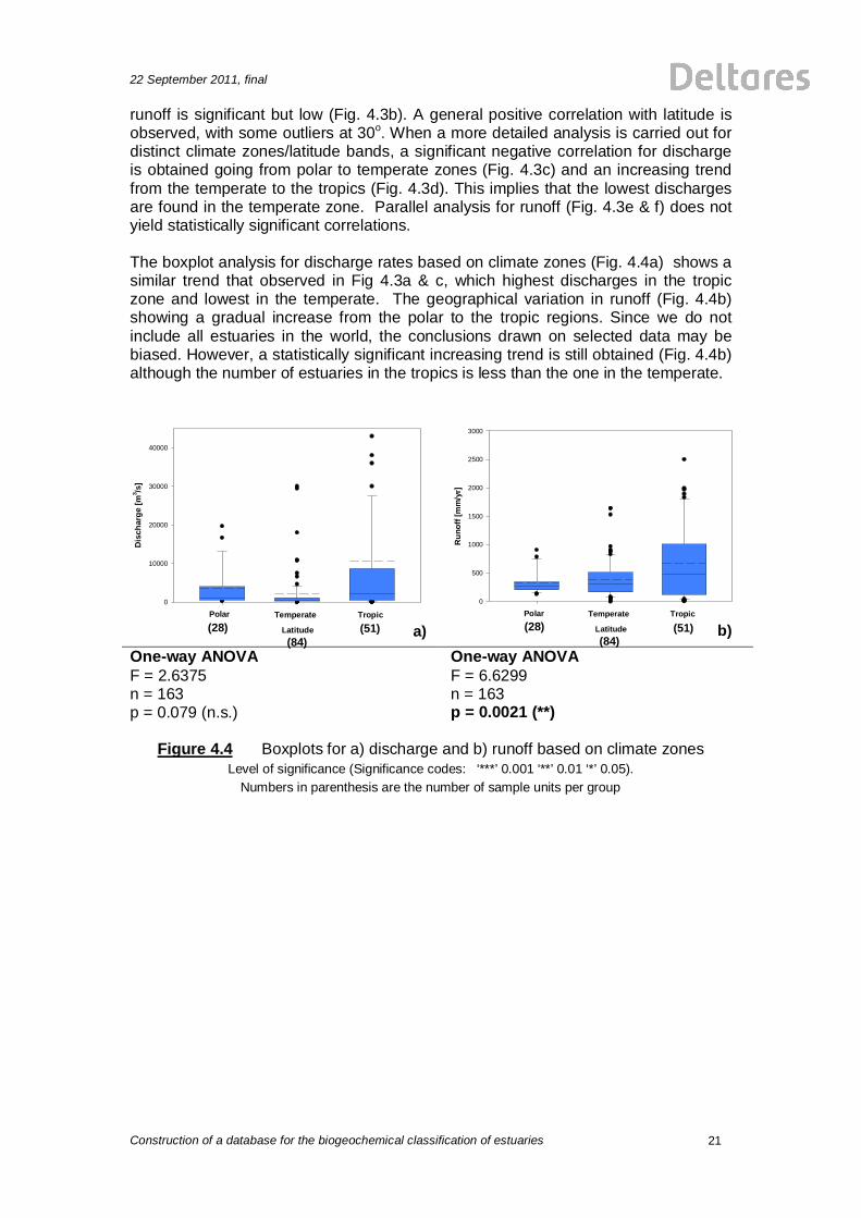
runoff is significant but low (Fig. 4.3b). A general positive correlation with latitude is observed, with some outliers at 30o. When a more detailed analysis is carried out for distinct climate zones/latitude bands, a significant negative correlation for discharge is obtained going from polar to temperate zones (Fig. 4.3c) and an increasing trend from the temperate to the tropics (Fig. 4.3d). This implies that the lowest discharges are found in the temperate zone. Parallel analysis for runoff (Fig. 4.3e & f) does not yield statistically significant correlations. The boxplot analysis for discharge rates based on climate zones (Fig. 4.4a) shows a similar trend that observed in Fig 4.3a & c, which highest discharges in the tropic zone and lowest in the temperate. The geographical variation in runoff (Fig. 4.4b) showing a gradual increase from the polar to the tropic regions. Since we do not include all estuaries in the world, the conclusions drawn on selected data may be biased. However, a statistically significant increasing trend is still obtained (Fig. 4.4b) although the number of estuaries in the tropics is less than the one in the temperate.
Latitude
Dis
char
ge [m
3 /s]
0
10000
20000
30000
40000
Polar Temperate Tropic
Latitude
Run
off [
mm
/yr]
0
500
1000
1500
2000
2500
3000
Polar Temperate Tropic
One-way ANOVA F = 2.6375 n = 163 p = 0.079 (n.s.)
One-way ANOVA F = 6.6299 n = 163 p = 0.0021 (**)
Figure 4.4 Boxplots for a) discharge and b) runoff based on climate zones
Level of significance (Significance codes: ‘***’ 0.001 ‘**’ 0.01 ‘*’ 0.05). Numbers in parenthesis are the number of sample units per group
(28) (84)
(51) (28) (84)
(51) a) b)

22
22 September 2011, final
Construction of a database for the biogeochemical classification of estuaries
4.2.2 Variation with estuarine shape/width convergence length
Estuarine Shape
Q (m
3 /s)
0
10000
20000
30000
40000
Funnel Mixed Prismatic
Estuarine shape
Run
off [
mm
/yr]
0
500
1000
1500
2500
3000
Funnel Mixed Prismatic
One-way ANOVA F = 1.4453, n = 114 p = 0.2424 (n.s.)
One-way ANOVA F = 0.4092, n = 114 p = 0.6658 (n.s.)
Figure 4.5 Boxplots for a) discharge and b) runoff in estuaries based on shape
Level of significance (Significance codes: ‘***’ 0.001 ‘**’ 0.01 ‘*’ 0.05). Numbers in parenthesis are the number of sample units per group
The statistical correlations obtained between discharge/runoff and estuarine shape are both mathematically insignificant (Figure 4.5a & b). However, a qualitative positive trend is observed between discharge and estuarine shape (Figure 4.5a) in which the prismatic-type estuaries are characterized by distinctly higher discharge rates (up to 5 times higher than funnel- and mixed-shaped). This observation can be directly linked to the combined outcome of Figure 4.2 and 4.3d, where the highest number of prismatic-shaped estuaries and the highest discharge rates are found in the tropics. Note that although these observations are based on the data available in the database, which does not include all estuaries world-wide, the observed trends are still significant. The number of prismatic- and funnel-shaped estuaries considered in Figure 4.5a is comparable, yet the mean discharge for prismatic-type is higher. The median runoff of the three categories is ~ 400-500 mm/yr (Figure 4.5b), implying that the differences in discharge based on estuarine shape are normalized when the basin area is taken into account. This implicitly means that basin area varies between the three different estuarine shape categories.
a) (43) (26)
(45) b) (43) (26)
(45)

22 September 2011, final
Construction of a database for the biogeochemical classification of estuaries
23
Discharge [m3/s]
0 500 1000 1500 2000
Wid
th c
onve
rgen
ce le
ngth
b [k
m]
0
10
20
30
40
50
60200400
Runoff [mm/yr]
0 500 1000 1500 2000 2500
Wid
th c
onve
rgen
ce le
ngth
b [k
m]
0
10
20
30
40
50
60200400
r = 0.3755 n = 115 p = 3.85e-5 (***)
r = 0.1104 n = 115 p = 0.2422 (n.s.)
Figure 4.6 Scatter plots and Spearman’s correlation for discharge/runoff agianst
width convergence length Level of significance (Significance codes: ‘***’ 0.001 ‘**’ 0.01 ‘*’ 0.05).
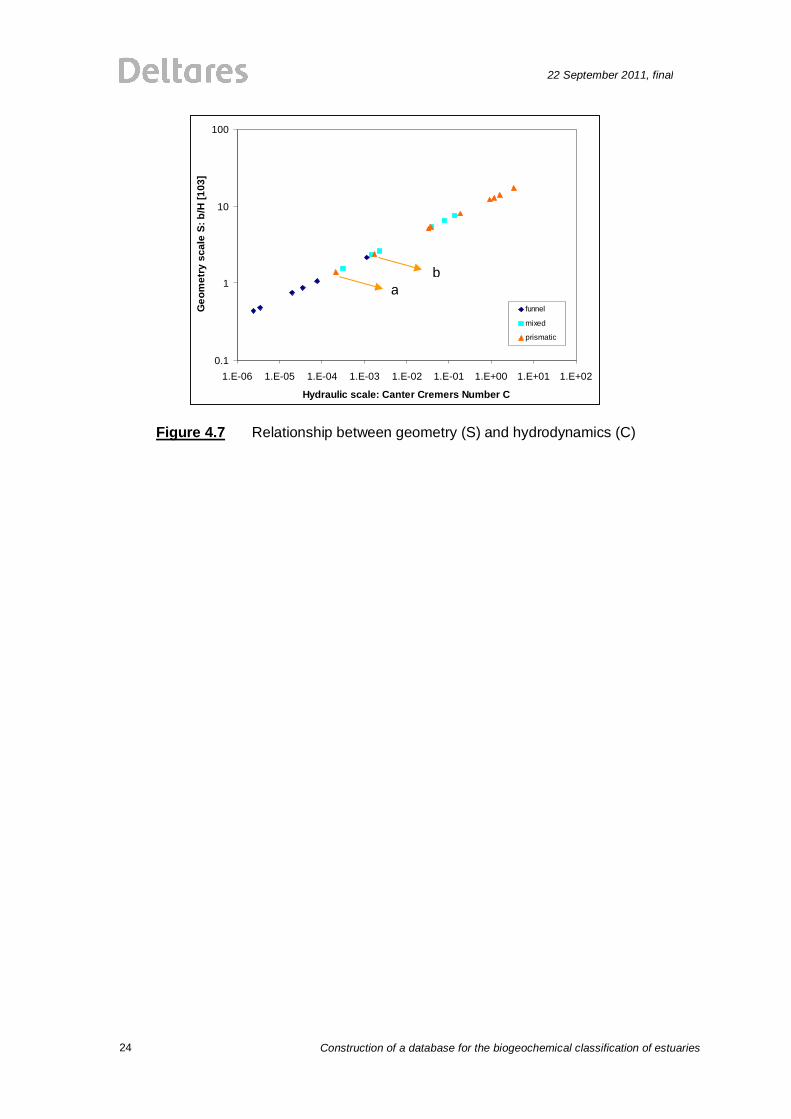
Figure 4.6a shows a positive significant correlation between discharge and the width convergence length of 115 estuaries. It is possible to identify that the funnel-shaped estuaries are mainly characterized by low discharges up to 500 m3/s, while the mixed and the prismatic shape estuaries exhibit a larger range of discharge rates. As in Figure 4.5b, there is no significant correlation among different estuarine shapes when runoff values are considered (Figure 4.6b). An alternative way to investigate the relation between the geometrical (estuarine shape or width convergence length) and hydrodynamic (discharge) features is through the relationship between the dimensionless estuarine shape number (S; Eq 3) and Canter-Cremers number (C; Eq 2). Based on the data available in our database, a clear trend is obtained between S and C (Figure 4.7), in which the funnel-shaped estuaries are characterized by low C and S values, whereas prismatic-shaped lie on the other end of the continuum. This is in line with the trend presented in Savenije (2006). Two outliers can be identified for the prismatic-shaped estuaries (a and b) exhibiting rather low S and C values. With a width convergence length value of 50 km, Anabar estuary (a) lies on the threshold between prismatic and mixed type estuaries. Kolyma Estuary (b) has a depth of 41.7 km, which is typically characteristic of funnel-shaped estuaries.
b) a)
funnel
mixed
prismatic
funnel
mixed
prismatic
24
22 September 2011, final
Construction of a database for the biogeochemical classification of estuaries
0.1
1
10
100
1.E-06 1.E-05 1.E-04 1.E-03 1.E-02 1.E-01 1.E+00 1.E+01 1.E+02
Hydraulic scale: Canter Cremers Number C
Geo
met
ry s
cale
S: b
/H [1
03]
funnel
mixed
prismatic
Figure 4.7 Relationship between geometry (S) and hydrodynamics (C)
a b

22 September 2011, final
Construction of a database for the biogeochemical classification of estuaries
25
4.3 Biogeochemical behavior The analysis of biogeochemical behavior based on the biogeochemical data collected in the database (Table 3.1) is performed by considering both substance concentrations (mg/l) and fluxes (Ton/yr, computed as the product of discharge and concentration). In what follows, the trends of the main chemical parameters (namely Si, DIN, DON, TN, DIP, DOC, POC and TSS) with geographical distribution (latitude/climate zones) and estuarine shape/convergence length are investigated. For the other biogeochemical parameters, such as DIC, PN, PP, the number of data entries is not sufficient for carrying out statistical analysis. Since the substance concentrations considered refer to the upper estuary where salinity is zero or close to zero, the trends based on estuarine shape cannot be directly related to biogeochemical behavior within estuaries. A summary of the statistical tests performed on the biogeochemical data is found in the Annex C. A list of additional statistical analyses of the other physico-chemical parameters can be found in Annex D.
4.3.1 Nutrient concentrations
A. Silica Silica
Latitude
-90-60-300306090
Si [m
g/l]
0.1
1
10
100
Polar Temperate Tropics PolarTemperate
Latitude
1 2 3
Si [m
g/l]
0
5
10
15
20
25
30
Polar Temperate Tropics
Spearman’s correlation r = -0.6448, n = 115 p = 7.37e-15 (***)
One-way ANOVA F = 29.1049, n = 115 p = 1.07e-9 (***) Silica
Latitude
-90-60-300306090
Si fl
ux [x
103 To
n/yr
]
1e-1
1e+0
1e+1
1e+2
1e+3
1e+4
1e+5
Polar Temperate Tropics PolarTemperate
a) b) (25) (61)
(29)
(25) (61)
(29) c) d)

26
22 September 2011, final
Construction of a database for the biogeochemical classification of estuaries
Spearman’s correlation r = -0.2915, n = 115 p = 0.0015 (**)
One-way ANOVA F = 2.3069, n = 115 p = 0.1091 (n.s.)
Convergence length b [km] 0 50 100 150 200 250 300 350
Si [m
g/l]
0,1
1
10
100
Estuary Shape
1 2 3
Si [m
g/l]
0
10
20
30
Funnel Mixed Prismatic
Spearman’s correlation r = 0.0062, n = 83 p = 0.9556 (n.s.)
One-way ANOVA F = 3.7396, n = 83 p = 0.0304 (*)
Convergence length b [km]
0 50 100 150 200 250 300 350
Si fl
ux [x
103 To
n/yr
]
1e-1
1e+0
1e+1
1e+2
1e+3
1e+4
1e+5
Estuary Shape
1 2 3
Si fl
ux [x
103 To
n/yr
]
0
1000
2000
3000
4000
5000
6000
70009000
10000
Funnel Mixed Prismatic
Spearman’s correlation r = 0.3240, n = 83 p = 0.0028 (**)
One-way ANOVA F=1.9303, n = 83 p = 0.1564 (n.s.)
Figure 4.8 Latitude/climate zones: a) & b) silica concentration [mg/l], c) & d) silica fluxes [x103Ton/yr];
Convergence length/estuarine shape: e) & f) silica concentration [mg/l], g) & h) silica fluxes [x103Ton/yr];
Level of significance (Significance codes: ‘***’ 0.001 ‘**’ 0.01 ‘*’ 0.05). Numbers in parenthesis refer to number sample units per group
In line with the study by Eyre and Balls (1999), Figure 4.8a and b show a distinct and statistically significant increase in Si concentrations from polar to the tropical region. A similar increasing trend is observed in Figure 4.8c, and to a lesser extent in Figure 4.8d, with Si fluxes increasing from the polar to tropical regions. In addition to higher discharge rates (Figure 4.3a), tropical zones are characterized by higher temperatures and therefore exhibit higher weathering rates. This leads to high Si fluxes (Figure 4.8c) and concentrations (Figure 4.8a), respectively. In the same way, Figure 4.8b and Figure 4.8d show a clear and gradual increase in silica fluxes and concentrations among the estuaries grouped per climate zone. This implies that Si concentrations vary proportionally to discharge rates, with highest Si concentrations in rivers with highest discharge rates, as is generally observed for
e) f)
g) h)
(27) (18)
(38)
(27) (18)
(38)

22 September 2011, final
Construction of a database for the biogeochemical classification of estuaries
27
substances resulting from weathering processes (Jolankai, 1992). Such a pronounced trend is observed despite the fact that the number of tropical estuaries in the analysis is only half of that from temperate zone and comparable to the number of estuaries in the polar region (Figure 4.8b & d). The trend in Si concentrations and fluxes with estuarine shape as determined by b, is less pronounced (Figure 4.8e-h). In terms of Si concentrations, the difference among the three climate groups is rather small even though a significant statistical correlation is obtained (Figure 4.8f). This result does not follow the observation drawn for Figure 4.8b, in which estuaries with high discharge rates (typically found in tropics or prismatic-shaped) also exhibit higher Si concentrations. The mean Si flux in the prismatic category is the highest, possibly attributed to the high discharge rates characteristic of prismatic estuaries (Figure 4.5a).
B. Dissolved Inorganic Nitrogen (DIN)
Latitude
-90-60-300306090
DIN
[mg/
l]
0.001
0.01
0.1
1
10
100
Polar Temperate Tropics PolarTemperate
Latitude
1 2 3
DIN
[mg/
l]
0
5
10
Polar Temperate Tropics
Spearman’s correlation r = -0.0651, n = 121 p = 0.4780 (n.s.)
One-way ANOVA F = 14.5821, n = 121 p = 4.77e-6 (***)
Latitude
-90-60-300306090
DIN
flux
[x 1
03 Ton/
yr]
0,1
1
10
100
1000
10000
Polar Temperate Tropics PolarTemperate
Spearman’s correlation r = -0.122, n = 121 p = 0.1825 (n.s.)
One-way ANOVA F = 0.9907, n = 121 p = 0.379 (n.s.)
a) b) (17) (69)
(35)
(17) (69)
(35) c) d)

28
22 September 2011, final
Construction of a database for the biogeochemical classification of estuaries
Convergence length b [km]
0 50 100 150 200 250 300 350
DIN
[mg/
l]
0,01
0,1
1
10
100
Estuary Shape
1 2 3
DIN
[mg/
l]
0
3
6
9
12
Funnel Mixed Prismatic
Spearman’s correlation r = -0.1758, n = 94 p = 0.090 (n.s.)
One-way ANOVA F = 5.5667, n = 94 p = 0.0070 (**)
Convergence length b [km]
0 50 100 150 200 250 300 350
DIN
flux
[x 1
03 Ton/
yr]
0,1
1
10
100
1000
Estuary Shape
1 2 3
DIN
flux
[x 1
03 Ton/
yr]
0
30
60
90
120
250
300
Funnel Mixed Prismatic
Spearman’s correlation r = 0.168, n = 94 p = 0.1054 (n.s.)
One-way ANOVA F = 1.7122, n = 94 p = 0.192 (n.s.)
Figure 4.9 Latitude/climate zones: a) & b) DIN concentration [mg/l], c) & d) DIN fluxes [x103Ton/yr];
Convergence length/estuarine shape: e) & f) DIN concentration [mg/l], g) & h) DIN fluxes [x103Ton/yr];
Level of significance (Significance codes: ‘***’ 0.001 ‘**’ 0.01 ‘*’ 0.05). Numbers in parenthesis refer to number sample units per group
Figure 4.9a and b show a significant difference in DIN concentration among the estuaries based on climate zones, with the highest DIN values found in the temperate area. Estuaries in North America and Europe located in the temperate zone are directly influenced by increased nutrient levels in rivers due to high anthropogenic activities, leading to DIN concentrations ~ two orders of magnitude higher than in the other climate zones. Such an inversed relation between concentration and discharge rates (high DIN concentrations in temperate zones with generally low discharge rates - Figure 4.3c & d; Fig 4.4a) is typically observed for substances released from point sources (Jolankai, 1992). When considering fluxes (Figure 4.9c & d), the high DIN concentrations in the temperate regions are compensated by the high discharge rates characteristic of tropical rivers (Figure 4.9d). This gives rise to a significantly higher median DIN flux in tropical area.
e) f)
g) h)
(33) (23)
(38)
(33) (23)
(38)

22 September 2011, final
Construction of a database for the biogeochemical classification of estuaries
29
The correlations between DIN concentration/fluxes and estuarine shape (Figure 4.9e-h) are generally not significant expect for Figure 4.9f which shows a general decrease in the mean DIN concentration from the funnel- to the prismatic-shaped estuaries. The factors contributing to the observed decrease cannot be readily identified based on the trend obtained in Figure 4.9f and the distribution of estuarine shapes among the different climate zones (Figure 4.2).
C. Dissolved Organic Nitrogen (DON)
Latitude
-90-60-300306090
DO
N [m
g/l]
0.001
0.01
0.1
1
10
100
Latitude
1 2 3D
ON
[mg/
l]0.0
0.5
1.0
1.5
2.06.0
7.0
8.0
Polar Temperate Tropics
Spearman’s correlation r = 0.4846, n = 60 p = 8.71e-5 (***)
One-way ANOVA F = 1.7426, n = 60 p = 0.1898 (n.s.) DON flux
Latitude
-90-60-300306090
DO
N fl
ux [x
103 To
n/yr
]
0.01
0.1
1
10
100
1000
10000
Latitude
1 2 3
DO
N fl
ux [x
103 To
n/yr
]
0
100
200
300
400
5001000
1100
1200
Polar Temperate Tropics
Spearman’s correlation r = 0.0597, n = 60 p = 0.6499 (n.s.)
One-way ANOVA F = 1.4691, n = 60 p = 0.2461 (n.s.)
a) b) (14) (29)
(20)
(14) (26)
(20) c) d)

30
22 September 2011, final
Construction of a database for the biogeochemical classification of estuaries
Convergence length b [km]
0 50 100 150 200 250 300 350
DO
N [m
g/l]
0,01
0,1
1
10
Estuarine shape
DO
N [m
g/l]
0.0
0.2
0.4
0.6
0.8
1.0
1.2
1.4
Funnel Mixed Prismatic
Spearman’s correlation r = -0.0039, n = 38 p = 0.9815 (n.s.)
One-way ANOVA F = 0.2951, n = 38 p = 0.7463 (n.s.)
Convergence length b [km]
0 50 100 150 200 250 300 350
DO
N fl
ux [x
103 To
n/yr
]
0,1
1
10
100
1000
10000
Estuarine shape
DO
N [x
103 To
n/yr
]
0
100
200
300
400
500
1000
1100
Funnel Mixed Prismatic
Spearman’s correlation r = 0.3768, n = 38 p = 0.0197 (*)
One-way ANOVA F = 1.8659, n = 38 p = 0.1790 (n.s.)
Figure 4.10 Latitude/climate zones: a) & b) DON concentration [mg/l],
c) & d) DON fluxes [x103Ton/yr]; Convergence length/estuarine shape: e) & f) DON concentration [mg/l],
g) & h) DON fluxes [x103Ton/yr]; Level of significance (Significance codes: ‘***’ 0.001 ‘**’ 0.01 ‘*’ 0.05).
Numbers in parenthesis refer to number sample units per group
The Spearman’s correlation test carried out to evaluate the relationship between DON concentration with latitude yields a statistically significant correlation (Figure 4.10a), although the corresponding One-way ANOVA is statistically insignificant (Figure 4.10b). An overall decrease in DON concentration can be observed from the polar-temperate zone to the tropic regions (Figure 4.10a). In terms of fluxes (Figure 4.10c & d), the general trend is reversed owing to the higher discharge rates in the tropics. The analysis of DON concentration with estuarine shape does not yield neither qualitative nor statistically significant correlations (Figure 4.10e & f). A significant correlation is obtained between DON flux and convergence length (Figure 4.10g) using the Spearman’s correlation test, showing higher fluxes in estuaries with higher convergence lengths, namely the prismatic estuaries (Figure 4.10h). The higher DON fluxes in tropical and prismatic-
e) f)
g) h)
(15) (7)
(16)
(15) (7)
(16)

22 September 2011, final
Construction of a database for the biogeochemical classification of estuaries
31
shaped groups can be attributed to higher discharge rates as well as higher predominance of prismatic-shaped estuaries in tropic regions (Figure 4.2). This is because the pronounced increase in tropic/prismatic-shaped groups (Figure 4.10d & h) is not observed for DON concentrations (Figure 4.10b & f).
D. Total Nitrogen (TN) TN concentration
Latitude
-90-60-300306090
TN [m
g/l]
0.001
0.01
0.1
1
10
100
Polar Temperate Tropics PolarTemperate
Latitude
1 2 3TN
[mg/
l]
0
2
4
6
8
12
14
Polar Temperate Tropics
Spearman’s correlation r = 0.1092, n = 137 p = 0.2041 (n.s.)
One-way ANOVA F = 10.5543, n = 137 p = 7.98e-5 (***) TN flux
Latitude
-90-60-300306090
TN fl
ux [x
103 To
n/yr
]
0.01
0.1
1
10
100
10000
Polar Temperate Tropics PolarTemperate
TN flux
Latitude
1 2 3
TN fl
ux [x
103 To
n/yr
]
0
100
200
300
400
500
6002000
2200
Polar Temperate Tropics
Spearman’s correlation r = -0.0580, n = 137 p = 0.4961 (n.s.)
One-way ANOVA F = 1.2320, n = 137 p = 0.4961 (n.s.)
a) b) (23) (76)
(38)
(23) (76)
(38) c) d)
32
22 September 2011, final
Construction of a database for the biogeochemical classification of estuaries
Convergence length b [km]
0 50 100 150 200 250 300 350
TN [m
g/l]
2
4
6
8
10
12
Estuarine shape
TN [m
g/l]
0
2
4
6
8
10
12
14
Funnel Mixed Prismatic
Spearman’s correlation r = -0.1961, n = 102 p = 0.0482 (*)
One-way ANOVA F = 5.3604, n = 102 p = 0.0085 (**)
Convergence length b [km]
0 50 100 150 200 250 300 350
TN fl
ux [x
103 To
n/yr
]
0,1
1
10
100
1000
10000
Estuarine shape
TN fl
ux [x
103 To
n/yr
]
0
100
200
300
400
500
600
700
Funnel Mixed Prismatic
Spearman’s correlation r = 0.1557, n = 102 p = 0.1182 (n.s.)
One-way ANOVA F = 1.5550, n = 102 p = 0.2207 (n.s.)
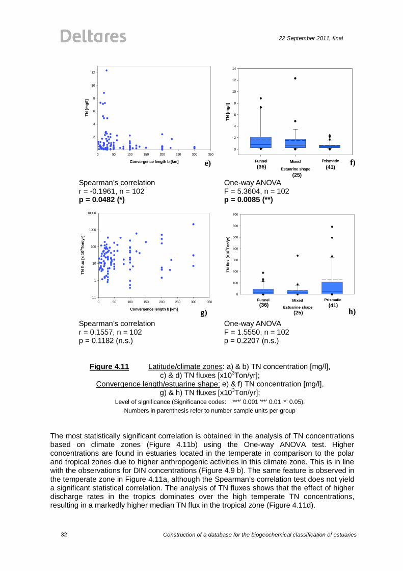
Figure 4.11 Latitude/climate zones: a) & b) TN concentration [mg/l], c) & d) TN fluxes [x103Ton/yr];
Convergence length/estuarine shape: e) & f) TN concentration [mg/l], g) & h) TN fluxes [x103Ton/yr];
Level of significance (Significance codes: ‘***’ 0.001 ‘**’ 0.01 ‘*’ 0.05). Numbers in parenthesis refer to number sample units per group
The most statistically significant correlation is obtained in the analysis of TN concentrations based on climate zones (Figure 4.11b) using the One-way ANOVA test. Higher concentrations are found in estuaries located in the temperate in comparison to the polar and tropical zones due to higher anthropogenic activities in this climate zone. This is in line with the observations for DIN concentrations (Figure 4.9 b). The same feature is observed in the temperate zone in Figure 4.11a, although the Spearman’s correlation test does not yield a significant statistical correlation. The analysis of TN fluxes shows that the effect of higher discharge rates in the tropics dominates over the high temperate TN concentrations, resulting in a markedly higher median TN flux in the tropical zone (Figure 4.11d).
e) f) (36) (25)
(41)
g) h) (36)
(25) (41)
22 September 2011, final
Construction of a database for the biogeochemical classification of estuaries
33
Figure 4.11e and f yield statistically significant negative correlations between TN concentrations and width convergence length/estuarine shape. A direct link between estuarine shape and concentration cannot be readily derived based on the Figure 4.11b and the distribution of estuarine shapes among the three climate zones (Figure 4.2). TN fluxes follow the opposite trend, with TN fluxes increasing going from funnel- to prismatic estuaries (Figure 4.11h). Estuaries with prismatic shapes show higher TN fluxes in comparison to the other estuarine shapes due to the contribution of high discharge rates in the tropics, where most of the prismatic estuaries are found (Figure 4.2). The overall trends observed in the analysis of TN concentrations and fluxes are similar to those for DIN. Also, the comparable DIN and TN concentrations and flux values imply that DIN is the most significant fraction of TN.
E. Dissolved Inorganic Phosphorus (DIP)
Latitude
-90-60-300306090
DIP
[mg/
l]
0.001
0.01
0.1
1
Polar Temperate Tropics PolarTemperate
Latitude
1 2 3
DIP
[mg/
l]
0.0
0.2
0.4
0.6
0.8
1.0
Polar Temperate Tropics
Spearman’s correlation r = -0.0163, n = 126 p = 0.8550 (n.s.)
One-way ANOVA F = 3.9704, n = 126 p = 0.0230 (*)
Latitude
-90-60-300306090
DIP
flux
[x 1
03 Ton/
yr]
0.1
1
10
100
1000
Polar Temperate Tropics PolarTemperate
Latitude
1 2 3
DIP
flux
[x 1
03 Ton/
yr]
0
20
40
150200
Polar Temperate Tropics
Spearman’s correlation r = -0.0809, n = 126 p = 0.3676 (n.s.)
One-way ANOVA F = 2.0514, n = 126 p = 0.1382 (n.s.)
a) b) (24) (67)
(35)
(24) (67)
(35) c) d)

34
22 September 2011, final
Construction of a database for the biogeochemical classification of estuaries
Convergence length b [km]
0 50 100 150 200 250 300 350
DIP
[mg/
l]
0,2
0,4
0,6
0,8
1,0
Estuary Shape
1 2 3
DIP
[mg/
l]
0.0
0.2
0.4
0.6
0.8
1.0
Funnel Mixed Prismatic
Spearman’s correlation r = -0.3134, n = 91 p = 0.0020 (**)
One-way ANOVA F = 3.7936, n = 91 p = 0.0304 (*)
Convergence length b [km]
0 50 100 150 200 250 300 350
DIP
flux
[x 1
03 Ton/
yr]
0,01
0,1
1
10
100
1000
Estuary Shape
1 2 3
DIP
flux
[x 1
03 Ton/
yr]
0
10
20
30
40
50
150
200
Funnel Mixed Prismatic
Spearman’s correlation r = 0.0651, n = 91 p = 0.5396 (n.s.)
One-way ANOVA F = 1.4062, n = 91 p = 0.2564 (n.s.)
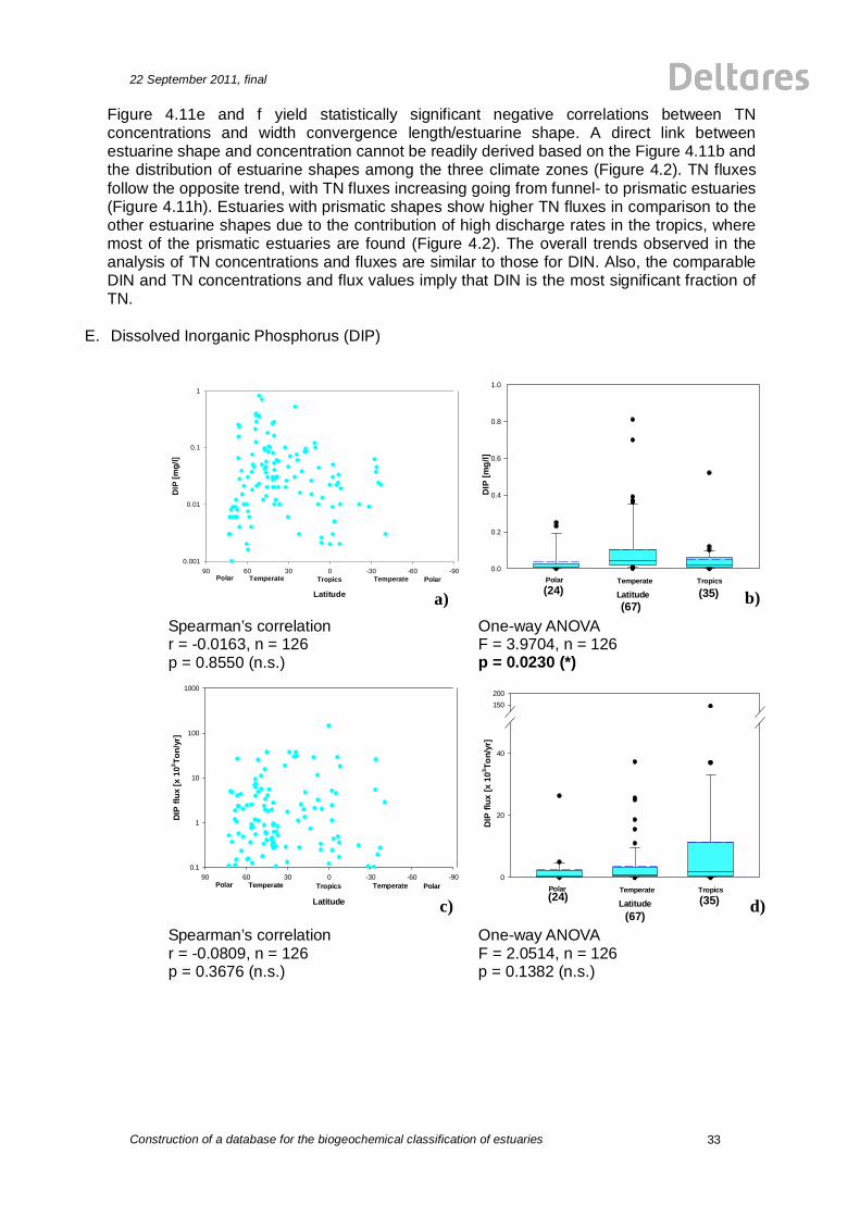
Figure 4.12 Latitude/climate zones: a) & b) DIP concentration [mg/l], c) & d) DIP fluxes [x103Ton/yr];
Convergence length/estuarine shape: e) & f) DIP concentration [mg/l], g) & h) DIP fluxes [x103Ton/yr];
Level of significance (Significance codes: ‘***’ 0.001 ‘**’ 0.01 ‘*’ 0.05). Numbers in parenthesis refer to number sample units per group
Figure 4.12a and b show that the highest DIP concentrations are found in temperate estuaries. As for nitrogen, this relates to the anthropogenic inputs in North American and European estuaries. The analysis of DIP fluxes with latitude/climate zones indicates higher DIP fluxes in tropical zones, followed by temperate and polar (Figure 4.12c & d), although the statistical correlations are not significant. Figure 4.12e and f show statistically significant negative correlations between DIP concentrations and estuarine shape, with higher DIP concentrations in funnel-shaped estuaries, decreasing towards the prismatic estuaries. The opposite trend is obtained in Figure 4.12g and h although the statistical tests do not show a significant correlation. In general, trends identified for DIP correspond to those observed for DIN (Figure 4.9) and TN (Figure 4.11).
e) f) (32) (22)
(37)
g) h) (32) (22)
(37)

22 September 2011, final
Construction of a database for the biogeochemical classification of estuaries
35
4.3.2 Carbon concentrations
A. Dissolved Organic Carbon (DOC)
Latitude
-90-60-300306090
DO
C [m
g/l]
0.001
0.01
0.1
1
10
100
Polar Temperate Tropics PolarTemperate
Latitude
1 2 3
DO
C [m
g/l]
0
5
10
15
20
25
Polar Temperate Tropics
Spearman’s correlation r = 0.1425, n = 84 p = 0.1950 (n.s.)
One-way ANOVA F = 2.6119, n = 84 p = 0.0930 (n.s.)
Latitude
-90-60-300306090
DO
C fl
ux [x
103 To
n/yr
]
1e-3
1e-2
1e-1
1e+0
1e+1
1e+2
1e+3
1e+4
1e+5
Polar Temperate Tropics PolarTemperate
Spearman’s correlation r = -0.1065, n = 84 p = 0.3346 (n.s.)
One-way ANOVA F = 4.0015, n = 84 p = 0.0321 (*)
a) b) (24) (67)
(35)
(24) (67)
(35) c) d)
36
22 September 2011, final
Construction of a database for the biogeochemical classification of estuaries
Convergence length b [km]
0 50 100 150 200 250 300 350
DOC
[mg/
l]
0,1
1
10
100
Estuary Shape
1 2 3
DO
C [m
g/l]
0
5
10
15
Funnel Mixed Prismatic
Spearman’s correlation r = 0.2589, n = 54 p = 0.0580 (n.s.)
One-way ANOVA F = 3.1528, n = 54 p = 0.0510 (n.s.)
Convergence length b [km]
0 50 100 150 200 250 300 350
DO
C fl
ux [x
103 To
n/yr
]
1e+0
1e+1
1e+2
1e+3
1e+4
1e+5
Estuary Shape
1 2 3
DO
C fl
ux [x
103 To
n/yr
]
0
500
1000
1500
2000
7600
7800
8000
Funnel Mixed Prismatic
Spearman’s correlation r = 0.3938, n = 54 p = 0.0030 (**)
One-way ANOVA F = 1.8300, n = 54 p = 0.1774 (n.s.)
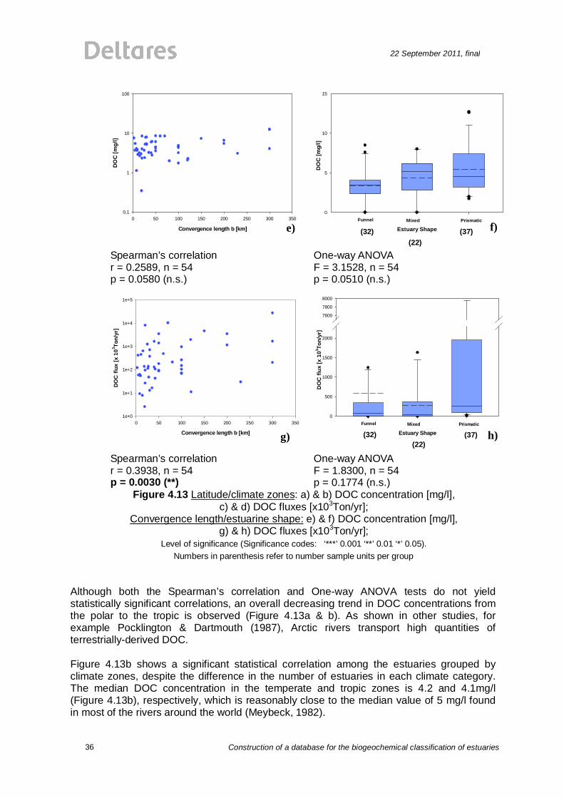
Figure 4.13 Latitude/climate zones: a) & b) DOC concentration [mg/l], c) & d) DOC fluxes [x103Ton/yr];
Convergence length/estuarine shape: e) & f) DOC concentration [mg/l], g) & h) DOC fluxes [x103Ton/yr];
Level of significance (Significance codes: ‘***’ 0.001 ‘**’ 0.01 ‘*’ 0.05). Numbers in parenthesis refer to number sample units per group
Although both the Spearman’s correlation and One-way ANOVA tests do not yield statistically significant correlations, an overall decreasing trend in DOC concentrations from the polar to the tropic is observed (Figure 4.13a & b). As shown in other studies, for example Pocklington & Dartmouth (1987), Arctic rivers transport high quantities of terrestrially-derived DOC. Figure 4.13b shows a significant statistical correlation among the estuaries grouped by climate zones, despite the difference in the number of estuaries in each climate category. The median DOC concentration in the temperate and tropic zones is 4.2 and 4.1mg/l (Figure 4.13b), respectively, which is reasonably close to the median value of 5 mg/l found in most of the rivers around the world (Meybeck, 1982).
e) f) (32) (22)
(37)
g) h) (32) (22)
(37)

22 September 2011, final
Construction of a database for the biogeochemical classification of estuaries
37
DOC fluxes show a generally increasing trend with latitude (Figure 4.13c). Although a higher median is observed for the tropics (Figure 4.13d), estuaries in the polar region show a higher DOC flux range. In the tropics, the high fluxes can be explained by the high discharge rates, whereas in polar regions, the observed high fluxes can be attributed to high DOC concentrations (Figure 4.13a & b). This is in line with generally high erosion rates for TOC (Pocklington & Dartmouth, 1987), of which DOC is the major fraction, characteristic of the Euroasian and the Soviet rivers of Siberia, included here in the polar category.
A generally increasing relation between DOC concentrations/fluxes and estuarine shape is observed (Figure 4.13e-h). A steady increase in DOC concentration is seen going from funnel- to prismatic-shaped estuaries although the correlation is not statistically significant (Figure 4.13f). The opposite trends obtained in the Figure 4.13b and Figure 4.13f cannot be explained based on available information. A statistically significant positive correlation between DOC fluxes and width convergence length is seen in Figure 4.13g, showing the highest DOC fluxes in prismatic-shaped estuaries (Figure 4.13h). This is related to the predominance of prismatic-shaped estuaries in tropical regions (Figure 4.2) which are generally characterized by high discharge rates (Figure 4.4).
B. Particulate Organic Carbon (POC)
Latitude
-90-60-300306090
PO
C [m
g/l]
0.1
1
10
100
1000
Polar Temperate Tropics PolarTemperate
Latitude
1 2 3
POC
[mg/
l]
0
5
10
15
20
25
Polar Temperate Tropics
Spearman’s correlation r = 0.1189, n = 50 p = 0.4105 (n.s.)
One-way ANOVA F = 0.6276, n = 50 p = 0.5541 (n.s.)
Latitude
-90-60-300306090
POC
flux
[x 1
03 Ton/
yr]
1e+0
1e+1
1e+2
1e+3
1e+4
1e+5
Polar Temperate Tropics PolarTemperate
Latitude
1 2 3
POC
flux
[x 1
03 Ton/
yr]
0
500
1000
1500
2000
2500
30005000
6000
Polar Temperate Tropics
a) b) (5) (25)
(20)
(5)
(25) (20) c) d)

38
22 September 2011, final
Construction of a database for the biogeochemical classification of estuaries
Spearman’s correlation r = -0.3066, n = 50 p = 0.0303 (*)
One-way ANOVA F = 0.76, n = 50 p = 0.4844 (n.s.)
Convergence length b [km]
0 50 100 150 200 250 300 350
POC
[mg/
l]
0,1
1
10
100
Estuarine shape
POC
[mg/
l]
0
20
40
60
80120
140
Funnel Mixed Prismatic
Spearman’s correlation r = 0.0174, n = 33 p = 0.9233 (n.s.)
One-way ANOVA F = 1.1413, n = 33 p = 0.3581 (n.s.)
Convergence length b [km]
0 50 100 150 200 250 300 350
POC
flux
[x 1
03 Ton/
yr]
1e+0
1e+1
1e+2
1e+3
1e+4
1e+5
Estuary Shape
1 2 3
POC
flux
[x 1
03 Ton/
yr]
0
500
1000
1500
2000
2500
3000
350010000
12000
Funnel Mixed Prismatic
Spearman’s correlation r = 0.4488, n = 33 p = 0.0087 (**)
One-way ANOVA F = 1.8301, n = 33 p = 0.2081 (n.s.)
Figure 4.14 Latitude/climate zones: a) & b) POC concentration [mg/l], c) & d) POC fluxes [x103Ton/yr];
Convergence length/estuarine shape: e) & f) POC concentration [mg/l], g) & h) POC fluxes [x103Ton/yr];
Level of significance (Significance codes: ‘***’ 0.001 ‘**’ 0.01 ‘*’ 0.05). Numbers in parenthesis refer to number sample units per group
As shown in Figure 4.14a and b, there is no significant relation between POC concentrations and latitude, although temperate estuaries show higher median concentrations in comparison to the polar and tropics. This could be possibly related to the anthropogenic activities in temperate estuaries, since polluted rivers and estuaries tend to have higher concentrations of POC. A positive statistical correlation is observed between POC flux and latitude (Figure 4.14c), which however is less visible in the analysis of climate groups (Figure 4.14d).
e) f) (13) (6)
(14)
g) h) (13) (6)
(14)

22 September 2011, final
Construction of a database for the biogeochemical classification of estuaries
39
POC fluxes exhibit a statistically significant trend with estuarine shape (Figure 4.14g), with values increasing going from the funnel- towards the prismatic-shaped estuaries. A steady increase in the median and range is also observed in Figure 4.14h, although the statistical correlation obtained by the One-way ANOVA test is not significant. The observed trends generally correspond to those identified for DOC concentrations and fluxes (Figure 4.13). The comparison of Figure 4.13 and Figure 4.14 shows that DOC concentrations are ~one order of magnitude higher than POC, as also stated in Olsson and Anderson (1997). DOC is also roughly comparable to TOC (not shown), implying that DOC is the major TOC fraction. This is generally true for all the estuaries in the database for which DOC and POC is available, except for Huang He estuary in which the POC concentration (132 mg/l) is 7.2 times higher than the DOC concentration.
4.3.3 Total Suspended Solids (TSS)
Latitude
-90-60-300306090
TSS
[mg/
l]
1e+1
1e+2
1e+3
1e+4
1e+5
Polar Temperate Tropics PolarTemperate
Latitude
1 2 3
TSS
[mg/
l]
0
2000
4000
6000
8000
Polar Temperate Tropics
Spearman’s correlation r = -0.4011, n = 127 p = 2.97e-6 (***)
One-way ANOVA F = 5.8102, n = 127 p = 0.0048 (**)
Latitude
-90-60-300306090
TSS
flux
[x 1
03 Ton/
yr]
1e+1
1e+2
1e+3
1e+4
1e+5
1e+6
1e+7
Polar Temperate Tropics PolarTemperate
Latitude
1 2 3
TSS
flux
[x 1
03 Ton/
yr]
0
5e+4
1e+5
2e+54e+55e+56e+5
Polar Temperate Tropics
Spearman’s correlation r = -0.4022, n = 127 p = 2.767e-6 (***)
One-way ANOVA F = 5.4022, n = 127 p = 0.006 (**)
a) b) (23) (67)
(37)
(23)
(67) (37) c) d)

40
22 September 2011, final
Construction of a database for the biogeochemical classification of estuaries
Convergence length b [km]
0 50 100 150 200 250 300 350
TSS
[mg/
l]
1e+0
1e+1
1e+2
1e+3
1e+4
1e+5
Estuary Shape
1 2 3
TSS
[mg/
l]
0
2500
5000
7500
1000025000
30000
Funnel Mixed Prismatic
Spearman’s correlation r = -0.0052, n = 87 p = 0.9615 (n.s.)
One-way ANOVA F = 0.2025, n = 87 p = 0.8173 (n.s.)
Convergence length b [km]
0 50 100 150 200 250 300 350
TSS
flux
[x 1
03 Ton/
yr]
1e+1
1e+2
1e+3
1e+4
1e+5
1e+6
1e+7
Estuary Shape
1 2 3
TSS
flux
[x 1
03 Ton/
yr]
0.0
5.0e+3
1.0e+4
1.5e+4
2.0e+4
1.0e+52.0e+53.0e+5
Funnel Mixed Prismatic
Spearman’s correlation r = 0.2694, n = 87 p = 0.0110 (*)
One-way ANOVA F = 1.4344, n = 87 p = 0.2492 (n.s.)
Figure 4.15 Latitude/climate zones: a) & b) TSS concentration [mg/l], c) & d) TSS fluxes [x103Ton/yr];
Convergence length/estuarine shape: e) & f) TSS concentration [mg/l], g) & h) TSS fluxes [x103Ton/yr];
Level of significance (Significance codes: ‘***’ 0.001 ‘**’ 0.01 ‘*’ 0.05). Numbers in parenthesis refer to number sample units per group
The analysis of TSS concentrations and fluxes with latitude yields statistically significant correlations (Figure 4.14a-d). A positive trend is obtained with increasing concentrations and fluxes going from the polar to tropical regions. The markedly high class range obtained for the tropical group (Figure 4.14d) indicates that the high fluxes are not only attributed to the high discharge rates (Figure 4.2) but also to high TSS concentrations (Figure 4.14b) characteristic for this climate zone. In line with previous results (e.g. silica; Figure 4.8), a combination of factors, namely high temperatures, high erosion and weathering rates, are the main contributing factors. The variations of TSS with estuarine shape are not statistically significant, with the exception of the Spearman’s correlation test for fluxes. The higher fluxes in estuaries with
e) f) (31) (20)
(36)
g) h) (31) (20)
(36)

22 September 2011, final
Construction of a database for the biogeochemical classification of estuaries
41
higher convergence length (Figure 4.14g) are attributed to the high discharge rates that generally characterize these estuaries (Figures 4.5a & 4.6a). However, the difference between the prismatic group and the other estuarine shapes is less pronounced in the box-plot analysis (Figure 4.14h).
5 Shortcomings
5.1 Physical and geometrical parameters In order to test the accuracy of our calculation, the methodology used here for the determination of the width convergence length (Section 3.2) was also applied to other estuaries for which the convergence length has been already measured and reported in other studies. A comparison of the calculated and previously available values of b (Table 5.1) shows that in most cases, b is on the same order of magnitude although not necessarily the same value. The difference in values can be related to the different applied methodologies. For instance, in GEMCO (2002) topographical maps available by that year were used as compared to this study, where satellite imagery maps available in Google Earth were used. This latter method provides an easier and more accurate way of measuring the widths and distances of estuaries. Other differences can be attributed to the dynamic nature of estuarine geomorphologies, for example in the measurement of the width at the mouth, especially in cases where the main river splits in several branches before discharging in the sea. Some examples of different estuaries that proved to be difficult to measure due to the presence of multiple mouths, branched main drainage lines and where main drainage lines form a bay are given in Annex B.
Table 5.1 Width convergence length calculated for some estuaries
convergence length b [km]
convergence length b [km] Estuary
From literature
Reference
This study
x [km] measured
Guadiana 9 GEMCO (2003) 15 20.14 Ebro 29 GEMCO (2003) 120 32.66 Mae Klong 155 Savenije (1992) 150 30.56
109 Savenije (2001) Chao Phya 56
Toffolon et al., (2006)
80 43.54
87 Savenije (2001) Tha Chin
50 Toffolon et al.,
(2006) 20 24.4
Loire 27 GEMCO (2003) 20 51.5 Eems 17 GEMCO (2003) 8 40.44
In this study we assume that the width convergence length (b) is equal to the cross-sectional convergence length (a). This major assumption is only valid for estuaries with a constant estuarine depth (h). Due to lack of bathymetric data for most estuaries in our database, this assumption was not further investigated. However, the distribution of the modeled a and b for a number of UK estuaries shows that a and b are not necessarily the same and hence the assumption of constant depth is not always valid.

42
22 September 2011, final
Construction of a database for the biogeochemical classification of estuaries
Figure 5.1 Distribution of width and area convergence length [m] along the discharge
[m3/s] of estuaries Source: Provided by Ian Townend, HR Wallingford Ltd
In a separate study on Australian estuaries, the difference in the measured convergence lengths can be attributed to the change of the geometry at the mouth. This change of the estuary mouth could be due to natural reasons in response to fresh water inflows and littoral drift, and anthropogenic structures. All these factors have an important implication for the water quality and ecology as well (Pierson et al., 2002).
5.2 Biogeochemical parameters These analyses rely on annual average concentrations and quantities and therefore do not give insight in the spatial and temporal variations.
6 Summary and outlook
A summary table with an overview of the significant statistical correlations between the tested chemical parameters and other factors included in the estuarine database (namely geographical distributions, climate zones, convergence length and estuary shape) is given in Table 6.1. Further details on the actual correlation indices are given in the Annex C.

22 September 2011, final
Construction of a database for the biogeochemical classification of estuaries
43
Table 6.1 Overview of the significant statistical correlations obtained for the variation in chemical parameters with respect to latitude/climate zone and width
convergence length/estuarine shape
Latitude Climate Convergence Estuary Parameter
(Spearman) Zones
(ANOVA) Length
(Spearman) Shape
(ANOVA)
Si
DIN
DON
TN
DIP
DOC
POC
TSS
flux concentration
According to the statistical results, it is possible to conclude that the geographical distribution and estuarine shape have some implications for the biogeochemical functioning of estuaries, in particular for Si, TN, DIP and TSS. In the analyses with latitude/climate zones, it became clear that climate plays an important role on the biogeochemical behavior of estuaries since most of the processes are temperature-dependant. Variation in discharge rates between the different climatic groups generally determines the trends in chemical fluxes. In the case of nutrients, anthropogenic activities characteristic to distinct climate zones greatly influence the concentration ranges. In general the following trends with latitude/climate zones have been identified:
Si, TSS concentrations/fluxes: increasing trend from polar to tropic DIN, DON, TN, DIP, POC concentrations: increasing from polar to temperate,
decreasing from temperate to tropic DIN, DON, TN, DIP fluxes: generally increasing from polar to tropic DOC concentrations: decreasing trend from polar to tropic
Si and TSS showed the most statistically significant correlations with positive trends for both concentrations and fluxes, increasing from the polar towards the tropics. Temperature-dependent erosion and weathering rates, as well as high discharge rates are the main characteristics of rivers located in the tropical region. In general, the highest nitrogen and phosphorus concentrations were observed in estuaries located in the temperate region, as a result of high anthropogenic activities in Europe and North America. Organic carbon in the form of DOC showed a negative trend decreasing from the polar to tropical zones. This is attributed to huge quantities of terrestrially-derived DOC transported by Arctic rivers to the Arctic Ocean. Concentrations of POC follow a similar trend as those

44
22 September 2011, final
Construction of a database for the biogeochemical classification of estuaries
established for nitrogen and phosphorus, in which the highest concentrations are found in the temperate regions as a result of anthropogenic activities. An important outcome is that substances resulting from erosion processes, such as Si and TSS vary directly with discharge, i.e. higher concentrations in rivers with higher discharges typically found in tropical regions. Substances possibly resulting from point sources, such as nutrients, vary inversely with discharges rates, i.e higher concentrations are found in rivers with generally lower discharges, such as in temperate regions. The identified trends with width convergence length/estuarine shape are less clear. This is because the values for chemical parameters in the database refer to the upper estuary characterized by salinities close to zero, whereas the estuarine shape is a characteristic of the lower estuary. Although it is not easy to establish a direct link with biogeochemical behavior, the concentration ranges and trends with estuarine shape will be used to define the upper estuarine boundary conditions in model scenarios that assume different estuarine shapes.
The following trends with width convergence length/estuarine shape have been identified:
Si, TSS concentration/fluxes: generally increasing from funnel- to prismatic-shaped DIN, TN, DIP concentrations: decreasing from funnel- to prismatic-shaped DIN, TN, DIP fluxes: increasing from funnel- to prismatic-shaped DOC, POC concentration/fluxes: generally increasing from funnel to prismatic
The classification and analysis of estuarine data presented above gives insight in the geometric-hydrodynamic-biogeochemical trends in estuaries world-wide. The trends and typical concentrations ranges established through data analysis will provide useful information for defining the hydrodynamic – biogeochemical estuarine modeling scenarios. The overall aim of the subsequent modeling study is to assess the contribution to CO2 air/water fluxes of estuaries, which be later upscaled from the regional scale to the global scale.

22 September 2011, final
Construction of a database for the biogeochemical classification of estuaries
45
7 References
Abril, G., A.V. Borges (2004). Greenhouse gas emissions: Fluxes and processes, Hydroelectric reservoirs and natural environments (Chapter 7: Carbon dioxide and methane emissions from estuaries). Berlin, Springler. Abril, G., H. Etcheber, B. Delille, M. Frankignoulle, A.V. Borges (2003). "Carbonate dissolution in the turbid and eutrophic Loire estuary." Marine Ecology Progress Series 259: 129-138. Abril, G., H. Etcheber, P. Le Hir, P. Bassoullet, B. Boutier, M. Frankignoulle (1999). "Oxic, anoxic oscillations and organic carbon mineralisation in an estuarine maximum turbidity zone (The Gironde, France)." Limnology and Oceanography 44(1304-1315). Abril, G., M. Nogueira, H. Etcheber, G. Cabecadas, E. Lemaire, M.J. Brogueira (2002). "Behaviour of organic carbon in nine contrasting european estuaries." Estuarine, Coastal and Shelf Science 54: 241-262. Anderson, L. G., K. Olsson, M. Chierici, (1998). "A carbon budget for the Artic Ocean." Global Biogeochemistry Cycles 12: 455-465. Arndt, S., J.P. Vanderborgth, P. Regnier, (2007). "Diatom growth response to physical forcing in a macrotidal estuary: Coupling hydrodynamics, sediment transport and biogeochemistry." Journal of Geophysical Research 12(doi:10.1029/2006JC003581). Arndt S., (2008). “Biogeochemical transformations and fluxes in redox-stratified environments: from the shallow coastal ocean to the deep subsurface” PhD Thesis, Utrecht University, Utrecht, The Netherlands. Azebedo, I., P. M. Duarte, A. A. Bordalo (2008). "Understanding spatial and temporal dynamics of key environmental characteristics in a mesotidal Atlantic estuary (Douro, NW Portugal)." Estuarine, Coastal and Shelf Science 76: 620-633. Balls, P. W. (1994). "Nutrient inputs to estuaries from nine scottish east coast rivers; influence of estuarine processes on inputs to the North Sea." Estuarine, Coastal and Shelf Science 39: 329-352. Bals, J. (2002). “Classification of European estuaries” M.Sc thesis, WL|Delft Hydraulics & TU Delft, The Netherlands. Beusekom, J. E. E., V.N. Jonge (1998). "Retention of phosphorus and nitrogen in the Ems Estuary." Estuaries 21(4A): 527-539. Borges, A. V. (2005). "Do we have enough pieces of the Jigsaw to intergrate CO2 fluxes in the coastal ocean?" Estuaries 28(1): 3-27. Borges, A. V., L.S. Schiettecatte, G. Abril, B. Delille, F. Gazeau (2006). "Carbon dioxide in European coastal waters." Estuarine, Coastal and Shelf Science 70: 375-387.

46
22 September 2011, final
Construction of a database for the biogeochemical classification of estuaries
Borges, A. V., M. Frankignoulle., (2002). "Distribution and air-water exchange of carbon dioxide in the Scheldt plume off the Belgian coast." Biogeochemistry 59: 41-67. Borges, A. V., Y.M. Kone, L.S. Schiettecatte, B. Delille, M. Frankignoulle, S. Bouillon (2005). Preliminary results on the biogeochemistry in the Mekong Estuary and delta (Vietnam). European Geosciences Union: 2nd General Assembly. Vienna - Austria, 24-29 April 2005. Bouillon, S., F. Dehairs, L. S. Schiettecatte, A. V. Borges (2007). "Biogeochemistry of the Tana estuary and delta (northern Kenya)." American Society of Limnology and Oceanography 52(1): 46-59. Bouillon, S., M. Frankignoulle, F. Dehairs, B. Velimirov, A. Eiler, G. Abril, H. Etcheber, A. V. Borges (2003). "Inorganic and organic carbon biogeochemistry in the Gautami Godavari estuary (Andhra Pradesh, India) during pre-monsoon: The local impact of extensive mangrove forests." Global Biogeochemical Cycles 17(4, doi:10.1029/2002GB002026): 1114. Bouwman, L., J. Harrison, S. Seitzinger, E. Mayorga (2010). Linking Watersheds to Coastal Marine Ecosystems: Global Nutrient River Export Trajectories 1970-2050. INPRINT. L.-O. I. i. t. C. Zone. Geesthacht, LOICZ IPO Institute for Coastal Research. Brasse, S., M. Nellen, R. Seifert, W. Michaelis (2002). "The carbon dioxide system in the Elbe estuary." Biogeochemistry 59: 25-40. Cabecadas, G., M. Nogueira, M. J. Brogueira (1999). "Nutrient Dynamics and Productivity in Three European Estuaries." Marine Pollution Bulletin 38(12): 1092-1096. Cai, W. J. (2003). "Riverine inorganic carbon flux and rate of biological uptake in the Mississippi River plume." Geophysical Research Letters 30(2): 1032 (doi:10.1029/2002GL016312). Cai, W. J., M. Daib, Y. Wanga, W. Zhaib, T. Huangb, S. Chenc, F. Zhangc, Z. Chenb, Z. Wang (2004). "The biogeochemistry of inorganic carbon and nutrients in the Pearl River estuary and the adjacent Northern South China Sea." Continental Shelf Research 24: 1301-1319. Cai, W. J., Y. Wang (1998). "The Chemistry, Fluxes, and Sources of Carbon Dioxide in the Estuarine Waters of the Satilla and Altamaha Rivers, Georgia." Limnology and Oceanography 43(4): 657-668. Cameron, W. M., D. W. Pritchard (1963). "Estuaries. In M. N. Hill (editor) " The Sea 2, John Wiley and Sons, New York: 306 - 324. Cauwet, G., F.T. Mackenzie (1993). "Carbon inputs and distribution in estuaries of turbid rivers: the Yang Tze and Yellow rivers (China)." Marine Chemistry 43: 235-246.

22 September 2011, final
Construction of a database for the biogeochemical classification of estuaries
47
Cole, J. J., N. F. Caraco (2001). "Carbon in catchments: connecting terrestrial carbon losses with aquatic metabolism." Institute of Ecosystem Studies 52: 101-110. Conley, D. J. (1997). "Riverine contribution of biogenic silica to the oceanic silica budget." American Society of Limnology and Oceanography 42(4): 774-777. CSIRO. (2003). "Simple Estuarine Response." from http://www.per.marine.csiro.au/serm2/interface?ozest:setEstuary=325,setView=map. Dagga, M., R. Bennerb, S. Lohrenzc, D. Lawrence (2004). "Transformation of dissolved and particulate materials on continental shelves influenced by large rivers: plume processes." Continental Shelf Research 24: 833-858. Dahm, C. N., S.V. Gregory, P.K. Park (1981). "Organic Carbon Transport in the Columbia River." Estuarine, Coastal and Shelf Science 13: 645-658. Dalrymple, R. W., B.A. Zaitlin, R. Boyd (1992). "Estuarine facies models: conceptual basis and stratigraphic implications." Journal of Sedimentary Petrology 62(6): 1130-1146. De la Paz, M., A. Gómez-Parra, J. Forja (2007). "Inorganic carbon dynamic and air–water CO2 exchange in the Guadalquivir Estuary (SW Iberian Peninsula)." Journal of Marine Systems 68: 265-277. De Mora, S. J. (1983). "The distribution of alkalinity and pH in the Frase Estuary." Environmental Technology 4(1): 35-46. DEFRA (2002). Safeguarding our seas, a strategy for the conservation and sustainable development of our marine environment London, Department for Environment, Food and Rural Affairs. Digby, M., P. Saenger, M.B. Whelan, D. McConchie, B. Eyre, N. Holmes, D. Bucher (1999). A Physical Classification of Australian Estuaries. LWRRDC Occasional Paper 16/99 (National River Health Program, Urban Sub–Program, Report No. 9) L. a. W. R. R. a. D. Corporation. Canberra ACT. July, ISSN 1320–0992, ISBN 0 642 26766 9. Eyre, B. D., P.W. Balls (1999). "A comparative study of nutrient processes along the salinity gradient of tropical and temperate estuaries." Estuaries 22: 313–326. Fox, L. E., F. Lipschultz, L. Kerkhof, S. C. Wofsy (1987). "A chemical survey of the Mississippi Estuary." Estuaries 10(1): 1-12. Frankignoulle, M., A. V. Borges, (2006(a)). Hydrochemistry measured on water bottle samples of first Douro cruise during BIOGEST. Mécanique des Fluides Géophysiques, Université de Liège, Publishing Network for Geoscientific & Environmental Data (PANGAEA). Frankignoulle, M., A.V. Borges (2006(b)). Hydrochemistry measured on water bottle samples of first Elbe cruise during BIOGEST. Mécanique des Fluides Géophysiques, Université de Liège Publishing Network for Geoscientific & Environmental Data (PANGAEA). Frankignoulle, M., A.V. Borges (2006(c)). Accompanying meteorological measurements for water bottle samples measured of third Gironde cruise during

48
22 September 2011, final
Construction of a database for the biogeochemical classification of estuaries
BIOGEST. Mécanique des Fluides Géophysiques, Université de Liège, Publishing Network for Geoscientific & Environmental Data (PANGAEA). Frankignoulle, M., A.V. Borges (2006(d)). Hydrochemistry measured on water bottle samples of first Loire cruise during BIOGEST. Mécanique des Fluides Géophysiques, Université de Liège, Publishing Network for Geoscientific & Environmental Data (PANGAEA). Frankignoulle, M., A.V. Borges (2006(e)). Hydrochemistry measured on water bottle samples of first Sado cruise during BIOGEST. Mécanique des Fluides Géophysiques, Université de Liège, Publishing Network for Geoscientific & Environmental Data (PANGAEA). Frankignoulle, M., A.V. Borges (2006(f)). Hydrochemistry measured on water bottle samples of third Scheldt cruise during BIOGEST. Mécanique des Fluides Géophysiques, Université de Liège, Publishing Network for Geoscientific & Environmental Data (PANGAEA). Frankignoulle, M., A.V. Borges (2006(g)). Hydrochemistry measured on water bottle samples of first Thames cruise during BIOGEST. Mécanique des Fluides Géophysiques, Université de Liège, Publishing Network for Geoscientific & Environmental Data (PANGAEA). Frankignoulle, M., A.V. Borges (2006(h)). Hydrochemistry measured on water bottle samples of fourth Rhine cruise during BIOGEST. Mécanique des Fluides Géophysiques, Université de Liège, Publishing Network for Geoscientific & Environmental Data (PANGAEA). Gattuso, J. P., M. Frankignoulle, R. Wollast., (1998). "Carbon and carbonate metabolism in coastal aquatic ecosystems." Annual Review Ecology Systematics 29: 405-433. GEMCO (2003). GEMCO - Estuary Classification and Scheldt Case Study, WL/Delt Hydraulics. Guo, X., W. J. Cai, W. Zhai, M. Dai, Y. Wang, B. Chen (2008). "Seasonal variations in the inorganic carbon system in the Pearl River (Zhujiang) estuary." Continental Shelf Research 28: 1424-1434. Gupta, G. V. M., S. D. Thottathil, K. K. Balachandran, N. V. Madhu, P. Madeswaran, S. Nair (2009). "CO2 Supersaturation and Net Heterotrophy in a Tropical Estuary (Cochin, India): Influence of Anthropogenic Effect." Ecosystems 12: 1145-1157. Harrison, J. A., N. Caraco, S.P. Seitzinger (2005(b)). "Global patterns and sources of dissolved organic matter export to the coastal zone: Results from a spatially explicit, global model." Global Biogeochemical Cycles 19 GB4S04, doi:10.1029/2005GB002480. Harrison, J. A., S.P. Seitzinger, A. F. Bouwman, N. F. Caraco, A. H.W. Beusen, C.J. Vorosmarty (2005(a)). "Dissolved inorganic phosphorus export to the coastal zone: Results from a spatially explicit, global model." Global Biogeochemical Cycles 19 (GB4S03, doi:10.1029/2004GB002357).

22 September 2011, final
Construction of a database for the biogeochemical classification of estuaries
49
Helie J.F., C. H. M., B. Rondeau (2002). "Seasonal changes in the sources and f luxes of dissolved inorganic carbon through the St. Lawrence River—isotopic and chemical constraint." Chemical Geology 186: 117-138. Hellings, L., F. Dehairs, S. Van Damme, W. Baeyens (2001). "Dissolved inorganic carbon in a highly polluted estuary (the Scheldt)." American Society of Limnology and Oceanography 46(6): 1406-1414. Holmes, R. M., B.J. Peterson, V.V. Gordeev, A.V. Zhulidov, M. Meybeck, R.B. Lammers, C.J. Vorosmarty (2000). "Flux of nutrients from Russian rivers to the Artic Ocean: Can we establish a baseline against which to judge future changes?" Water Resources Research 36(8): 2309-2320. Holmes, R. M., J. Peterson, V. V. Gordeev, A. V. Zhulidov, M. Meybeck, R. B. Lammers, C. J. Vorosmarty (2000). "Flux of nutrients from Russian rivers to the Arctic Ocean: Can we establish a baseline against which to judge future changes?" Water Resources Research 36(8): 2309-2320. Howland, R. J. M., A.D. Tappin, R.J. Uncles, D.H. Plummer, N.J. Bloomer (2000). "Distributions and seasonal variability of pH and alkalinity in the Tweed Estuary, UK." The Science of the total Environment 251-252: 125-138. Hume, T. M., C.E. Herdendorf (1988). "A geomorphic classification of estuaries and its application to coastal resource management - A New Zealand example" Journal of Ocean and Shoreline Management 11: 249-274. Hume, T. M., T. Snelder, M. Weatherhead, R. Liefting (2007). “A controlling factor approach to estuary classification” Ocean & Coastal Management 50: 905-929. Jay, D. A., W.R. Geyer, D.R. Montgomery (2000). En ecological perspective on estuarine classification. In: Hobbie, J.E. (Ed.), Estuarine science: A synthetic approach to research and practice. Island, Washington DC. Jolankai, G. (1992). “, chemical and biological processes of contaminant transformation and transport in river and lake systems. A state-of-art review”, IHP-IV Projects H-3.2 Technical Documents in Hydrology, International Hydrological Programme, UNESCO, Paris, 1992. Kaldy, J. E., L.A. Cifuentes, D. Brock (2005). "Using Stable Isotope Analyses to Assess Carbon Shallow Subtropical Estuary." Estuaries 28(1): 86-95. Kromkamp, J., J. Peene, P. van Rijswijk, A. Sandee, N. Goosen (1995). "Nutrients, light and primary production by phytoplankton and microphytobenthos in the eutrophic, turbid Westerschelde estuary (The Netherlands)." Hydrobiologia 311: 9-19. Langbein, W. B. (1963). "The hydraulic geometry of a shallow estuary." Bulletin of International Association of Scientific Hydrology 8: 84-94. Lanzoni, S., G. Seminara (1998). "On tide propagation in convert estuaries." Journal of Geophysical Research 103(C13): 30: 793-812. Laurelle G.G. (2009). “Quantifying nutrient cycling and retention in coastal waters at the global scale”. Ph.D thesis, Utrecht University, Utrecht, The Netherlands, No. 312

50
22 September 2011, final
Construction of a database for the biogeochemical classification of estuaries
Lebo, M. E. (1991). "Particle-bound phosphorus along an urbanized coastal plain estuary." Marine Chemistry 34: 225-246. Lewis, W. M., S.K. Hamilton, J.F. Saunders (1995). Rivers of northern South America (Chp. 8), Elsiever. Liu, S. M., G.H. Hong, X. W. Ye, J. Zhang, X. L. Jiang (2009). "Nutrient budgets for large Chinese estuaries and embayment." Biogeosciences Discussion 6: 391-435. Meybeck, M. (1982). "Carbon, nitrogen and phosphorus transport by world rivers." American Journal Science 282: 401-450. Meybeck, M. (1993). "C, N, P and S in rivers: from sources to global inputs. In interactions of C, N, P and S Biogeochemical cycles and global change." NATO ASI Series, Springer-Verlag 14: 163-191. Meybeck, M., A. Ragu (1995). River Discharges to Oceans: An assessment of suspended solids, major ions and nutrients, UNEP. Meybeck, M., C.J. Vorosmarty (2005). "Fluvial filtering of land to ocean fluxes: from natural Holocene variations to anthropocene. ." Comptes Rendus Geoscience 337(1-2): 107-123. Meybeck, M., G. Cauwet, S. Dessery, M. Somville, D. Gouleaud, G. Billen (1988). "Nutrients (Organic C,P,N,Si) in the eutrophic River Loire (France) and its Estuary." Estuarine, Coastal and Shelf Science 27: 595-624. Mitchell, & Stapp, (1992). Field Manual for Water Quality Monitoring. Milliman, J. D., C. Rutkowski, M. Meybeck (1995). River Discharge to the Sea, A Global River Index (GLORI), LOICZ Core Project Office, Netherland Institute for Sea Research (NIOZ). Mortazavi, B., R. L. Iverson, W. Huang (2001). "Dissolved organic nitrogen and nitrate in Apalachicola Bay, Florida: spatial distributions and monthly budgets." Marine Ecology Progress Series 214: 79-91. Mortazavi, B., R. L. Iverson, W. Huang, F. G. Lewis, J. M. Caffrey (2000). "Nitrogen budget of Apalachicola Bay, a bar-built estuary in the northeastern Gulf of Mexico." Marine Ecology Progress Series 195: 1-14. Neal, C., W. A. House, H.P. Jarvie, A. Eatherall (1998). "The significance of dissolved carbon dioxide in major lowlands rivers entering the North Sea." The Science of the total Environment 210/211: 187-203. NEEA, N. E. E. A. (1999). "NEEA Estuaries Database" from http://ian.umces.edu/neea/siteinformation.php. Nikiforov, S. L., R. Colony, L. Timokhov (2008). Hydrochemical Atlas of the Arctic Ocean. Arctic and Antarctic Research Institute of the Russian Federal Service for Hydrometeorology and Environmental Monitoring, International Arctic Research Center, University of Alaska Publishing Network for Geoscientific & Environmental Data (PANGAEA).

22 September 2011, final
Construction of a database for the biogeochemical classification of estuaries
51
Olsson, K., L. G. Anderson (1997). “Input and biogeochemical transformation of dissolved carbon in the Siberian shelf seas” Continental Shelf Research 17: 819-833. OZCoasts. (2010). "Australian Online Coastal Information." from http://www.ozcoasts.org.au/search_data/simple_search.jsp. Pages, J., J. Lemoalle, B. Fritz (1995). "Distribution of Carbon in a Tropical Hypersaline Estuary, The Casamance (Senegal, West Africa)." Estuaries 18(3): 456-468. Park, P. K., M. Catalfomo, G.R. Webster, B.H. Reid (1970). "Nutrients and carbon dioxide in the Columbia River." Pastuszaka, M., Z. Witekb, K. Nagelc, M. Wielgata, A. Grelowski (2005). "Role of the Oder estuary (southern Baltic) in transformation of the riverine nutrient loads." Journal of Marine Systems 57: 30-54. Peterson, B. J., R.M. Holmes, J.W. McClelland, C.J. Vorosmarty, R.B. Lammers, A.I. Shiklomanov, I.A. Shiklomanov, S. Rahmstorf (2002). "Increasing river discharge to the Arctic Ocean." Science 298: 2171-2173. Pethick, J. (1984). An Introduction to Coastal Geomorphology. London, Edward Arnold Publishers. Pierson, W. L., K. Bishop, D. Van Senden, P.R. Horton, C.A. Adamantidis (2002). Environmental water requirements to maintain estuarine processes, Environmental flows iniciative technical report Number 3. Commonwealth of Australia. Canberra. Pillsbury, G., Ed. (1956). Tidal Hydraulics. Vicksburg, USA. Pocklington, R., Dartmouth (1987). "Arctic Rivers and their discharges" Mitt. Geol.-Palaont. Inst. Univ. Hamburg SCOPE/UNEP Sonderbd., (64): 261-268. Pritchard, D. (1967). "What is an estuary: physical viewpoint, In: Lauff GH (Ed.)." Estuaries, American Association for the Advancement of Science: 3-5. Pritchard, D. W. (1955). "Estuarine circulation patterns. ." Proceedings of the American Society of Civil Engineers 81 (no 717): 1 - 11. Raymond, P. A., N. F. Caraco, J. J. Cole (1997). "Carbon Dioxide Concentration and Atmospheric flux in the Hudson River." Estuaries 20(2): 381-390. Richey, J. E., J. M. Melack, A. K. Aufdenkampe, V. M. Ballester, L. L. Hess (2002). "Outgassing from Amazonian rivers and wetlands as a large tropical source of atmospheric CO2." Letters to Nature 416: 617-620. Robson, B. J., P.A. Buckaveckas, D.P. Hamilton (2008). "Modelling and mass balance assessments of nutrient retention in a seasonally-flowing estuary (Swan River Estuary, Western Australia)." Estuarine, Coastal and Shelf Science 76: 282-292.

52
22 September 2011, final
Construction of a database for the biogeochemical classification of estuaries
Sanders, R. J., T. Jickells, S. Malcolm, J. Brown, D. Kirkwood, A. Reeve, J. Taylor, T. Horrobin, C. Ashcroft (1997). "Nutrient fluxes through the Humber estuary." Journal of Sea Research 37: 3-23. Savenije, H. H. G. (1992). Rapid assessment technique for salt intrusion in alluvial estuaries. Delft, Technische Universiteit Delft. PhD thesis. Savenije, H. H. G. (2001). "A simple analytical expression to describe tidal damping or amplification " Journal of Hydrology 243: 205-215. Savenije, H. H. G. (2005). Salinity and Tides in Alluvial Estuaries. Delft, ELSEVIER BV. Seitzinger, S. P., E. Mayorga, A.F. Bouwman, C. Kroeze, A.H.W. Beusen, G. Billen, G. Van Drecht, E. Dumont, B.M. Fekete, J. Garnier (2010). "Global river nutrient export: A scenario analysis of past and future trends." Global Biogeochemistry Cycles 24: GB0A08, doi:10.1029/2009GB003587. Seitzinger, S. P., J.A. Harrison (2008). Nitrogen in the marine environment (Chapter 9: Land-Base nitrogen sources and their delivery to coastal systems), Elsevier Inc. Semiletov, I. P. (1999). "Aquatic Sources and Sinks of CO2 and CH4 in the Polar Regions." Journal of the Atmospheric Sciences 56: 286-306. Soetaert, K., J. J. Middelburg, C. Heip, P.Meire, S. Van Damme, T. Maris (2006). "Long-term change in dissolved inorganic nutrients in the heterotrophic Scheldt estuary (Belgium, The Netherlands)." American Society of Limnology and Oceanography 51(1, part 2): 409-423. Stalnackea, P., A. Grimvallb, C. Libisellerb, M. Laznikc, I. Kokorited (2003). "Trends in nutrient concentrations in Latvian rivers and the response to the dramatic change in agriculture." Journal of Hydrology 283: 184-205. Swaney, D. P., D. Scavia, R.W. Howarth, R.M. Marino (2008). “Estuarine classification and response to nitrogen loading: Insights from simple ecological models” Estuarine, Coastal and Shelf Science 77: 253-263 The Estuary Guide. (2009). "Estuary guide." from http://www.estuary-guide.net/search/estuaries/details.asp?fileid=82. Toffolon, M., G. Vignoli, M. Tubino (2006). "Relevant parameters and finite amplitude effects in estuarine hydrodynamics." Journal Geophysical Res., 111(C10014, doi: 10.1029/2005JC003104). Toffolon, M., H.H.G. Savenije. (2008). "DBest, a databse of estuarine morphology." from http://www.ing.unitn.it/~toffolon/dbest/index.htm. Uncles, R. J., R. G. Wood, J. A. Stephens, R. J. M. Howland (1998). "Estuarine Nutrient Fluxes to the Humber Coastal Zone, UK, during June 1995." Marine Pollution Bulletin 37(3-7): 225-233. UNEP/MAP (2003). Riverine transport of water, sediments and pollutants to the Mediterranean Sea. MAP technical reports Series No. 141. Athens, United Nations Environment Programme/Mediterranean Action Plan (UNEP/MAP).

22 September 2011, final
Construction of a database for the biogeochemical classification of estuaries
53
Van der Zee, C., N. Roevros, L. Chou (2007). "Phosphorus speciation, transformation and retention in the Scheldt estuary (Belgium/The Netherlands) from the freshwater tidal limits to the North Sea." Marine Chemistry Article in press. Williams, A., C. F. Herbert, J. Pethick, K. Dyer, A. Williams (2001). The Estuaries Research Programme, Phase 1, Predictive methods Report, Ministry of Agriculture, Fisheries & Food (MAFF), Environment Agency English Nature. Yao, G., Q. Gao, Z. Wang, X. Huang, T. He, Y. Zhang, S. Jiao, J. Ding (2007). "Dynamics of CO2 partial pressure and CO2 outgassing in the lower reaches of the Xijiang River, a subtropical monsoon river in China." Science of the Total Environment 376: 255-266. Zhai, W., M. Dai, X. Guo (2007). "Carbonate system and CO2 degassing fluxes in the inner estuary of Changjiang (Yangtze) River, China." Marine Chemistry 107: 342-356. Zhaia, W., M. Daia, W. J. Caic, Y. Wang, Z. Wang (2005). "High partial pressure of CO2 and its maintaining mechanism in a subtropical estuary: the Pearl River estuary, China." Marine Chemistry 93: 21-32. Zwolsman, J. J. G. (1994). North Sea estuaries as filters for contaminants, Delft Hydraulics: 129.

54
22 September 2011, final
Construction of a database for the biogeochemical classification of estuaries
ANNEX A
Information About Estuaries US Environmental Protection Agency (EPA)
EPA Office of Water Resource Center (OWRC) Operated by The Track Group
NOTE: This information resource includes links to non-EPA web sites mention of these web sites, organizations, or services should not be considered an endorsement
by EPA.
“Estuaries are places where rivers meet the sea. Estuaries are critical to the health of coastal environments and to our enjoyment of them. EPA's National Estuary Program was established by Congress in 1987 to improve the quality of estuaries of national
importance.”
[Source: http://www.epa.gov/owow/estuaries/]
National Estuary Program (NEP)
++ Home ++ http://www.epa.gov/owow/estuaries/
Basic Information About Estuaries http://www.epa.gov/owow/estuaries/about.html Challenges http://www.epa.gov/owow/estuaries/challenges.html Climate Ready Estuaries (CREs)
http://epa.gov/cre/
Basic Information http://www.epa.gov/cre/basic.html
Coastal Toolkit http://www.epa.gov/cre/toolkit.html
Explore http://www.epa.gov/cre/explore.html
News and Events http://www.epa.gov/cre/news.html
Where You Live http://www.epa.gov/cre/live.html
Contact Us http://www.epa.gov/owow/estuaries/contact.html EPA's 2004-2006 National Estuary Program (NEP) Implementation Report http://www.epa.gov/owow/estuaries/pdf/2004-2006_irreportfinal_6-19-08.pdf Estuaries and Clean Water Act of 2000
http://www.epa.gov/owow/estuaries/pdf/s835_estuaries2000.pdf

22 September 2011, final
Construction of a database for the biogeochemical classification of estuaries
55
Estuaries in the National Estuary Program http://www.epa.gov/owow/estuaries/estuaries.html
Contact Information http://www.epa.gov/owow/estuaries/contactinfo.html
Comprehensive Conservation and Management Plans (CCMPs) http://www.epa.gov/owow/estuaries/ccmp/index.html
Home Pages http://www.epa.gov/owow/estuaries/nep_home.html
Profiles http://www.epa.gov/owow/estuaries/profiles.html
Study Areas http://www.epa.gov/owow/estuaries/studyareas.html
Watersheds http://www.epa.gov/owow/estuaries/watersheds.html
Exploring Estuaries [Content for children, students & teachers] http://www.epa.gov/owow/estuaries/kids/ Frequently Asked Questions (FAQs) http://www.epa.gov/owow/estuaries/questions.html Habitat Protection & Restoration Overview http://www.epa.gov/owow/estuaries/pivot/overview/intro.htm
Contributing Factors http://www.epa.gov/owow/estuaries/pivot/overview/factors.htm
Habitat Goals and NEP Plans http://www.epa.gov/owow/estuaries/pivot/habitat/doing.htm
Habitat Loss and Degradation http://www.epa.gov/owow/estuaries/pivot/habitat/problem.htm
Local NEP Projects and Regional Summary http://www.epa.gov/owow/estuaries/pivot/habitat/hab_fr.htm
National Program Results http://www.epa.gov/owow/estuaries/pivot/habitat/progress.htm
National Coastal Condition Report III (2008) http://www.epa.gov/owow/oceans/nccr3/downloads.html National Estuary Program Booklet
http://www.epa.gov/owow/estuaries/pdf/nep_brochure_timeless_new.pdf National Estuary Program Evaluation Guidance http://www.epa.gov/owow/estuaries/pdf/final_guidance_sept28.pdf National Estuary Program in Action
http://www.epa.gov/owow/estuaries/action.html National Program Results http://www.epa.gov/owow/estuaries/pivot/habitat/progress.htm Smart Growth: Estuary Programs and Improvement http://www.epa.gov/owow/estuaries/smartgrowth.html

56
22 September 2011, final
Construction of a database for the biogeochemical classification of estuaries
State of Our NEP Estuaries http://www.epa.gov/owow/estuaries/bay.html Videos from the National Estuary Programs http://www.epa.gov/owow/estuaries/nepvideos.html Chesapeake Bay Program Office [The Chesapeake Bay is protected under its own federally mandated program, separate but related to the National Estuary Program] ++ Home ++ http://www.epa.gov/Region3/chesapeake/ Bay Barometer: A Health and Restoration Assessment of the Chesapeake Bay and Watershed in 2008
http://www.chesapeakebay.net/content/publications/cbp_34915.pdf Chesapeake Bay Program
http://www.chesapeakebay.net/ Civil Enforcement
http://www.epa.gov/compliance/civil/initiatives/chesapeakebay.html Contacts
http://www.chesapeakebay.net/comments.aspx Oceans, Coasts & Estuaries ++ Home ++ http://www.epa.gov/OWOW/oceans/index.html A – Z Index http://www.epa.gov/owow/oceans/a-z.html General Information & Resources http://www.epa.gov/owow/oceans/geninfo.html Ocean Regulatory Programs http://www.epa.gov/owow/oceans/regulatory/index.html Related Information Resources National Oceanic & Atmospheric Administration (NOAA) ++ Home ++
http://www.noaa.gov/index.html Estuaries http://oceanservice.noaa.gov/education/tutorial_estuaries/welcome.html Estuaries.Gov http://www.estuaries.gov/

22 September 2011, final
Construction of a database for the biogeochemical classification of estuaries
57
Further Reading
http://oceanservice.noaa.gov/education/tutorial_estuaries/est12_references.html Resources
http://www.estuaries.gov/estuaries101/Resources/Home.aspx What is an Estuary?
http://oceanservice.noaa.gov/education/tutorial_estuaries/est01_whatis.html Where We Work http://www.estuaries.gov/estuaries101/About/Default.aspx?ID=349

58
22 September 2011, final
Construction of a database for the biogeochemical classification of estuaries
ANNEX B
Rhine and Schedlt Estuaries
Brahmaputra Estuary
L=15 km
L=20 km

22 September 2011, final
Construction of a database for the biogeochemical classification of estuaries
59
Appachicola Estuary
Amazon Estuary
L=250 km
L=5 km

60
22 September 2011, final
Construction of a database for the biogeochemical classification of estuaries
ANNEX C
Table C1: Summary statistics for biogeochemical features (fluxes) among the estuaries clustered by climate zone and shape
Parameter flux
sampling sites grouped by test F/t /r - value n p - value Signific.
One-way ANOVA 2.3069 115 0.1091 n.s. Geographical distribution
Spearman’s corr. -0.2915 115 0.0015 * * One-way ANOVA 1.9303 83 0.1564 n.s.
Estuarine shape Spearman’s corr. 0.3240 83 0.0028 * *
Si
Tropics t - test 0.5547 29 0.5837 n.s. One-way ANOVA 0.9907 121 0.379 n.s.
Geographical distribution Spearman’s corr. -0.122 121 0.1825 n.s. One-way ANOVA 1.7122 94 0.192 n.s.
Estuarine shape Spearman’s corr. 0.168 94 0.1054 n.s.
DIN
Tropics t - test 1.0246 35 0.3153 n.s. One-way ANOVA 1.4691 60 0.2461 n.s.
Geographical distribution Spearman’s corr. 0.0597 60 0.6499 n.s.
Tropics t - test 0.1789 20 0.86 n.s. One-way ANOVA 1.8659 38 0.1790 n.s.
DON
Estuarine shape Spearman’s corr. 0.3768 38 0.0197 * One-way ANOVA 1.232 137 0.299 n.s.
Geographical distribution Spearman’s corr. -0.058 137 0.4961 n.s.
Tropics t - test 0.7518 38 0.458 n.s. One-way ANOVA 1.5550 102 0.2207 n.s.
TN
Estuarine shape Spearman’s corr. 0.1557 102 0.1182 n.s. One-way ANOVA 2.0514 126 0.1382 n.s.
Geographical distribution Spearman’s corr. -0.0809 126 0.3676 n.s. One-way ANOVA 1.4062 91 0.2564 n.s.
Estuarine shape Spearman’s corr. 0.0651 91 0.5396 n.s.
DIP
Tropics t - test 1.5778 35 0.1277 n.s. One-way ANOVA 4.0015 84 0.0321 *
Geographical distribution Spearman’s corr. -0.1065 84 0.3346 n.s. One-way ANOVA 1.8300 54 0.1774 n.s.
Estuarine shape Spearman’s corr. 0.3938 54 0.0030 * *
DOC
Tropics t - test -0.0227 26 0.9821 n.s. One-way ANOVA 0.76 50 0.4844 n.s.
Geographical distribution Spearman’s corr. -0.3066 50 0.0303 * One-way ANOVA 1.8301 33 0.2081 n.s.
Estuarine shape Spearman’s corr. 0.4488 33 0.0087 * *
POC
Tropics t - test 0.5088 20 0.6171 n.s. One-way ANOVA 5.4022 127 0.006 * *
Geographical distribution Spearman’s corr. -0.4022 127 2.767e-6 * * * One-way ANOVA 1.4344 87 0.2492 n.s.
TSS
Estuarine shape Spearman’s corr. 0.2694 87 0.0110 *

22 September 2011, final
Construction of a database for the biogeochemical classification of estuaries
61
Tropics t - test 0.6883 37 0.4968 n.s. Level of significance (Significance codes: ‘***’ 0.001 ‘**’ 0.01 ‘*’ 0.05).
Table C2: Summary statistics for biogeochemical features (concentrations) among the estuaries clustered by climate zone and shape
Parameter
concentration sampling sites grouped by
test F /r - value n p - value Signific.
One-way ANOVA 29.1049 115 1.07e-9 * * * Geographical distribution
Spearman’s corr. -0.6448 115 7.37e-15 * * * One-way ANOVA 3.7396 83 0.0304 *
Si Estuarine shape
Spearman’s corr. 0.0062 83 0.9556 n.s. One-way ANOVA 14.5821 121 4.77e-6 * * *
Geographical distribution Spearman’s corr. -0.0651 121 0.4780 n.s. One-way ANOVA 5.5667 94 0.0070 * *
DIN Estuarine shape
Spearman’s corr. -0.1758 94 0.0900 n.s. One-way ANOVA 1.7426 60 0.1898 n.s.
Geographical distribution Spearman’s corr. 0.4846 60 8.71e-5 * * * One-way ANOVA 0.2951 38 0.7463 n.s.
DON Estuarine shape
Spearman’s corr. -0.0039 38 0.9815 n.s. One-way ANOVA 10.5543 137 7.98e-5 * * *
Geographical distribution Spearman’s corr. 0.1092 137 0.2041 n.s. One-way ANOVA 5.3604 102 0.0085 * *
TN Estuarine shape
Spearman’s corr. -0.1961 102 0.0482 * One-way ANOVA 3.9704 126 0.0230 *
Geographical distribution Spearman’s corr. -0.0163 126 0.8550 n.s. One-way ANOVA 3.7936 91 0.0304 *
DIP Estuarine shape
Spearman’s corr. -0.3134 91 0.0020 * * One-way ANOVA 2.6119 84 0.0930 n.s.
Geographical distribution Spearman’s corr. 0.1425 84 0.1950 n.s. One-way ANOVA 3.1528 54 0.0510 n.s.
DOC Estuarine shape
Spearman’s corr. 0.2589 54 0.0580 n.s. One-way ANOVA 0.6276 50 0.5541 n.s.
Geographical distribution Spearman’s corr. 0.1189 50 0.4105 n.s. One-way ANOVA 1.1413 33 0.3581 n.s.
POC Estuarine shape
Spearman’s corr. 0.0174 33 0.9233 n.s. One-way ANOVA 5.8102 127 0.0048 * *
Geographical distribution Spearman’s corr. -0.4011 127 2.97e-6 * * * One-way ANOVA 0.2025 87 0.8173 n.s.
TSS Estuarine shape
Spearman’s corr. -0.0052 87 0.9615 n.s. Level of significance (Significance codes: ‘***’ 0.001 ‘**’ 0.01 ‘*’ 0.05).

62
22 September 2011, final
Construction of a database for the biogeochemical classification of estuaries
ANNEX D
Estuarine Shape
Latit
ude
-40
-20
0
20
40
60
80
Funnel Mixed Prismatic
Geographical distribution
b (k
m)
0
100
200
300
Polar Temperate Tropic
One-way ANOVA F = 0.5373, n = 116 p = 0.5858 (n.s.)
One-way ANOVA F = 2.6929, n = 115 p = 0.0721 (n.s.)
Latitude
-60 -30 0 30 60 90
Con
verg
ence
leng
th b
(km
)
1
10
100
1000
Spearman’s correlation r = -0.006, n = 117 p = 0.9448 (n.s.)
Latitude
HC
O3
(mg/
l)
0
100
200
300
400
Polar Temperate Tropics
Latitude
-60 -30 0 30 60 90
HCO
3 (m
g/l)
1
10
100
1000
One-way ANOVA F = 12.8436, n = 125 p = 1.59e-5 (***)
Spearman’s correlation r = -0.0557, n = 125 p = 0.5374 (n.s.)
a) b) (41) (26)
(49) (18) (66)
(31)
c)
d) e) (25) (66)
(34)

22 September 2011, final
Construction of a database for the biogeochemical classification of estuaries
63
Estuarine Shape
HC
O3
(mg/
l)
0
100
200
300
400
Funnel Mixed Prismatic
Convergence length b [km]
0 50 100 150 200 250 300 350
HCO
3 (m
g/l)
1
10
100
1000
One-way ANOVA F = 4.38, n = 91 p = 0.0154 (*)
Spearman’s correlation r = -0.2664, n = 91 p = 0.0107 (*)
Latitude
Tota
l alk
alin
ity [
mol
/l]
0
500
1000
1500
2000
2500
Temperate Tropics
Latitude
-60 -30 0 30 60 90
Tota
l alk
alin
ity (
mol
/l)
0,001
0,01
0,1100
1000
10000
t-test t = 0.3996, n = 22 p = 0.6937 (n.s.)
Spearman’s correlation r = -0.1414, n = 23 p = 0.5200 (n.s.)
Estuarine Shape
Tota
l alk
alin
ity (
mol
/l)
0,00
0,01
0,021000,002000,00
Funnel Mixed Prismatic
Convergence length b [km]
0 50 100 150 200 250 300 350
Tota
l alk
alin
ity (
mol
/l)
0,001
0,01
0,1100
1000
10000
One-way ANOVA F = 3.1011, n = 20 p = 0.0937 (n.s.)
Spearman’s correlation r = 0.2741, n = 20 p = 0.2422 (n.s.)
f) g) (31) (21)
(39)
h) i) (15) (7)
j) k) (7) (4)
(9)

64
22 September 2011, final
Construction of a database for the biogeochemical classification of estuaries
Latitude
pH
6,0
6,5
7,0
7,5
8,0
8,5
9,0
Temperate Tropics
Latitude
-60 -30 0 30 60 90
pH
6
7
8
9
10
t-test t = -1.0462, n = 19 p = 0.3101 (n.s.)
Spearman’s correlation r = 0.0752, n = 20 p = - (n.s.)
Estuarine Shape
pH
6,5
7,0
7,5
8,0
8,5
9,0
Funnel Mixed Prismatic
Convergence length b [km]
0 50 100 150 200 250 300 350
pH
6
7
8
9
10
One-way ANOVA F = 0.0379, n = 17 p = 0.9629 (n.s.)
Spearman’s correlation r = 0.1064, n = 17 p = - (n.s.)
Latitude
Air-
wat
er C
O2_
flux
[mol
C/m
2 /yr]
0
20
40
60
80
100
Temperate Tropics
Latitude
-60 -30 0 30 60
Air-
wat
er C
O2_
flux
[mol
C/m
2 /yr]
0
10
20
30
40
50
60
70
80
90
t-test t = 1.0180, n = 15 p = 0.3272 (n.s.)
Spearman’s correlation r = 0.4179, n = 15 p = 0.1227 (n.s.)
l) m) (14) (5)
n) o) (8) (4)
(5)
p) q) (12) (3)

22 September 2011, final
Construction of a database for the biogeochemical classification of estuaries
65
Estuarine Shape
Air-
wat
er C
O2_
fluxe
s (m
olC
/m2 /y
r)
0
20
40
60
80
100
Funnel Mixed Prismatic
Convergence length b [km]
0 50 100 150 200 250 300 350
Air-
wat
er C
O2_
flux
[mol
C/m
2 /yr]
0
10
20
30
40
50
60
70
80
90
100
One-way ANOVA F = 1.6445, n = 14 p = 0.2372 (n.s.)
Spearman’s correlation r = -0.4775, n = 14 p = 0.0842 (n.s.)
r) s) (6) (5)
(3)


22 September 2011, final
Construction of a database for the biogeochemical classification of estuaries
67
ANNEX E
Hydro-morphological characteristics
Temp Basin Area Discharge ho Bo Ao Ho b Ls Ts Lat Long oC (km2) (km3 yr-1) (m) (m) (m2) (m) (km) (km) (km) River Continent a b c g h j k l m n o p
References
Alabama N.America 56894 g=2;
Altamaha N.America 31.39N 81.50W 23.8 35224 10.8 1.96 3500 50 a,b,h=1; g=2; c,j=33; k,n=calc
Amazon S.America 0.10N 49.00W 27 6112000 6590 149000 300 a,b,c,h=1; g=2; k,n=calc
Amguema Asia 68.1N 177.40W 29600 9.2 a,b,h=1; g=2
Amur Asia 53.10N 140.44E -1 1748000 344 15000 200 a,b,c,h=1; g=2; k,n=calc
Anabar Asia 73.14N 113.35E 98550 13.2 28000 50 a,b,h=1; g=2; k,n=calc
Appalachicola N.America 30.42N 84.52W 23.7 44548 21.43 1.81 800 40 a,b,h=1; g=2; c,j=33; k,n=calc
Apure S.America 8N 70W 170000 72.5328 a,b=8; g=2;h=10 Aux Outar N.America 49.09N 68.24W 191000 a,b=1; g=2;
Balsas N.America 17.55N 102.10W 122600 14 600 40 a,b,h=1; g=2;k,n=calc
Barito Asia 3.32S 114.29E 66000 86.8 12700 40 a,b,h=1; g=2; k,n=calc
Brahmaputra Asia 23.42N 90.22E 15.3 580000 510 24400 40 a,b,c,h=1; g=2; k,n=calc
Brazos N.America 29.35N 95.45W 23.9 116568 5.04 4.62 700 35 a,b,h=1; g=2; c,j=33; k,n=calc
Bug Europe 47.33N 30.47E 68980 3.4 a,b,h=1; g=2 Caroni S.America 6N 63W 95000 157.68 a,b=8; i=10; g=2
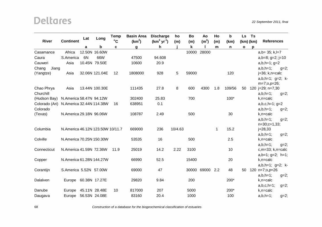
68
22 September 2011, final
Construction of a database for the biogeochemical classification of estuaries
Temp Basin Area Discharge ho Bo Ao Ho b Ls Ts Lat Long oC (km2) (km3 yr-1) (m) (m) (m2) (m) (km) (km) (km) River Continent a b c g h j k l m n o p
References
Casamance Africa 12.50N 16.60W 10000 28000 a,b= 35; k,l=7 Caura S.America 6N 66W 47500 94.608 a,b=8; g=2; j=10 Cauweri Asia 10.45N 79.50E 10600 20.9 a,b,h=1; g=2 Chang Jiang (Yangtze) Asia 32.06N 121.04E 12 1808000 928 5 59000 120
a,b,h=1; g=2; j=36; k,n=calc
Chao Phrya Asia 13.44N 100.30E 111435 27.8 8 600 4300 1.8 109/56 50 120
a,b,h=1; g=2; k-m=7;o,p=26; j=29; n=7,30
Churchill (Hudson Bay) N.America 58.47N 94.12W 302400 25.83 700 100*
a,b,h=1; g=2; k,n=calc
Colorado (Ari) N.America 32.44N 114.38W 16 638951 0.1 a,b,c,h=1; g=2 Colorado (Texas) N.America 29.18N 96.06W 108787 2.49 500 30
a,b,h=1; g=2; k,n=calc
Columbia N.America 46.12N 123.50W 10/11.7 669000 236 10/4.63 1 15.2
a,b,h=1; g=2; n=30;c=1,33; j=28,33
Colville N.America 70.25N 150.30W 53535 16 500 2.5 a,b,h=1; g=2; k,n=calc
Connecticut N.America 41.59N 72.36W 11.9 25019 14.2 2.22 3100 10 a,b,h=1; g=2; c,m=33; k,n=calc
Copper N.America 61.28N 144.27W 66990 52.5 15400 20 a,b=1; g=2; h=1; k,n=calc
Corantijn S.America 5.52N 57.00W 69000 47 30000 69000 2.2 48 50 120 a,b,h=1; g=2; k-n=7;o,p=26
Dalalven Europe 60.38N 17.27E 29820 9.84 200 200* a,b,h=1; g=2; k,n=calc
Danube Europe 45.11N 28.48E 10 817000 207 5000 200* a,b,c,h=1; g=2; k,n=calc
Daugava Europe 56.53N 24.08E 83160 20.4 1000 100 a,b,h=1; g=2;

22 September 2011, final
Construction of a database for the biogeochemical classification of estuaries
69
Temp Basin Area Discharge ho Bo Ao Ho b Ls Ts Lat Long oC (km2) (km3 yr-1) (m) (m) (m2) (m) (km) (km) (km) River Continent a b c g h j k l m n o p
References
k,n=calc
Delaware N.America 40.13N 74.47W 12.1 29500 15.3 5.8/6.12 37655 255000 1.5 42/54 140 200
a,b,h=1; c=33; g=2; k-m=7; o,p=26; j=28,33; n=7,30
Dnepr Europe 46.30N 32.18E 504000 53.4 5400 100* a,b,h=1; g=2; k,n=calc
Dnestr Europe 46.10N 30.19E 77000 10.7 7000 20 a,b,h=1; g=2; k,n=calc
Don Europe 47.15N 39.45E 422000 20.7 200 3.7 50 a,b,h=1; g=2; m=37; k,n=calc
Douro Europe 41.09N 8.37W 22.6 95000/115320 15.6 6 800 4800 2.8/ 1-3 29 30.3
a,b,h=1; c=38; g=1,5; j-o=3; m=3,5
Drammenselva Europe 59.44N 10.15E 17000 8.1 2800 30 a,b,h=1; g=2; k,n=calc
Ebro Europe 40.49N 0.31E 84000 9.24 6.8 1500 10200 0.6 29 46.6 a,b=1; g=2; h=4; j-o=3
Eems Europe 53.30N 9.00E 5100/9000 1.9 3.9 12000 46800 3.6/ 2-3 17 61
a,b,h=1; g=1,5; j-o=3, m=3,5; k,n=7
Elbe Europe 53.50N 7.00E 8.78 146000/145800 23.7 13.5 17250 232875 3.3/ 2-3 20/56 93.6
a,b,h=1; g=2,5; j-o=3; m=3,5; c=39; n=3,30
Evros Europe 40.53N 26.10E 55000 9.81 500 40 a,b,h=1; g=2; k,n=calc
Fraser N.America 49.23N 121.27W 4 220000 111.9528 9 4.6 a,b,c,h=1; g=2; ;j=28; n=30
Fuchun Jiang Asia 30.18N 120.07E 54349 37.3 27300 60 a,b,h=1; g=2; ; k,n=calc

70
22 September 2011, final
Construction of a database for the biogeochemical classification of estuaries
Temp Basin Area Discharge ho Bo Ao Ho b Ls Ts Lat Long oC (km2) (km3 yr-1) (m) (m) (m2) (m) (km) (km) (km) River Continent a b c g h j k l m n o p
References
Gambia Africa 13.31N 14.50W 42000 4.9 8.7 9687 84400 1.2 121/56/40 300 500
a,b,h=1; g=2; k-m,p=7,o=26; j=29; n=7,29,30
Ganges Asia 24.05N 89.02E 18 1050000 493 a,b,c,h=1; g=2
Garonne Europe 44.25N 0.14E 55000 17.2 23400 40 a,b,h=1; g=2; k,n=calc
Gironde Europe 45.6N -1.1E 23.44 71000 28.3824 10 14000 140000 4.5/ 2-5 33/87 100
a,b=6; g=5; j-l,o,p=3; m=3,5; c=40; n=3,30
Glama Europe 59.36N 11.07E 47310 19.9 800 80 a,b,h=1; g=2; k,n=calc
Godavari Asia 16.55N 81.47E 29 312000 105 3300 80* a,b,c,h=1; g=2; k,n=calc
Grijalva N.America
(MX) 18.36N 92.39W 36400 23 1600 30 a,b,h=1; g=2; k,n=calc
Guadiana Europe 37.13N 7.24W 72000 9 1.5 1450 2175 3.2 9 15.5 a,b,h=1; g=2; j-o=3
Gualdalquivir Europe 37.31N 5.59W 56000 7.29 2 6750 13500 3.2 16 37.9 a,b,h=1; g=1; j-o=3
Guaviare S.America 4N 69W 150000 274.3632 a,b=8; g=2; j=10
Huang He Asia 37.44N 118.36E 13 752000 41 2 1800 100* a,b,c,h=1; g=2; j=36; k,n=calc
Hudson N.America 40.42N 74.02W 12.4 34700 17.3 9.2/6.13 42
a,b,h=1; c=33; g=2; j=28,33; n=30
Humber Europe 53.60N 0.10E 24240 9.271584 19 12000 228000 8 20 109 a,b=41; j-o=3; g=42
Hunter Australia 32.55S 151.46E 21411 1.65 2 3.1 a,b,h=1; g=2; j,m=32

22 September 2011, final
Construction of a database for the biogeochemical classification of estuaries
71
Temp Basin Area Discharge ho Bo Ao Ho b Ls Ts Lat Long oC (km2) (km3 yr-1) (m) (m) (m2) (m) (km) (km) (km) River Continent a b c g h j k l m n o p
References
Incomati Africa 25.46S 32.43E 46200 2.3 3 4500 8100 2.7 42/5.5 50 100
a,b,h=1; g=1; k-m=7; o,p=26; j=29; n=7,30
Indigirka Asia 70.39N 147.50E -12 362000 61 6900 30 a,b,c,h=1; g=2; k,n=calc
Indus Asia 25.23N 68.24E 18.8 916000 57 4200 60 a,b,h=1; g=2; k,n=calc
Japura S.America 2S 68W 300000 567.648 a,b=8; g=2 Jurua S.America 5S 68W 220000 204.984 a,b=8; g=2
Kamchatka Asia 56.14N 162.28E 50370 33.1 2400 30 a,b,h=1; g=2; k,n=calc
Khatanga Asia 72.55N 106.00E 364000 85.3 23300 130 a,b,h=1; g=2; k,n=calc
Klamath N.America 41.31N 123.58W 12.2 31339 15.2 2.81 2700 8 a,b,h=1; g=2; c,j=33; k,n=calc
Kobuk N.America 66.45N 161.00W 24657 16 a,b,h=1; g=2
Kolyma Asia 68.34N 160.58E -9 663200 132 14200 100 a,b,h=1; g=2; k,n=calc
Kuban Europe 45.16N 162.27W 57900 13.4 a,b,h=1; g=2 Kuskowin N.America 60.17N 162.27W 80549 60 a,b,h=1; g=2 Kymjoki Europe 60.30N 26.52E 37200 9.68 a,b,h=1; g=2
Lalang Asia 2.38S 104.66E 10.6 350 2550 2.7 96/217/60 65 200
a,b=7; k-n=6; o,p=26; j=29; n=29,30
Lena Asia 70.42N 127.39E -9 2490000 525 21000 200* a,b,c,h=1; g=2; k,n=calc
Liao Asia 40.50N 121.48E 7 232000 16.2 10800 12 a,b,c,h=1; g=2; k,n=calc
Limpopo Africa 25.15S 33.30E 21 440000 26 7 371 2600 1.1 50/215 60 150 a,b,c,h=1; g=1; k-m=7; o,p=26;

72
22 September 2011, final
Construction of a database for the biogeochemical classification of estuaries
Temp Basin Area Discharge ho Bo Ao Ho b Ls Ts Lat Long oC (km2) (km3 yr-1) (m) (m) (m2) (m) (km) (km) (km) River Continent a b c g h j k l m n o p
References
j=29; n=7,30
Loire Europe 47.16N 2.11W 19.5 112000/115000 26 13 12750 165750 5.1/ 3-6 27 102
a,b,h=1; g=2,5; j-o=3; m=3,5; c=43
Luan Asia 39.20N 119.10E 54000 4.2 a,b,h=1; g=2 Maas (Meuse) Europe 65.50N 44.20E 29000 10.2 a,b,g,h=1
MacKenzie N.America 68.16N 133.40W -4 1787000 308 10700 50 a,b,c,h=1; g=2; k,n=calc
Madeira S.America 8 S 62W 1300000 946.08 a,b=8; g=2
Mae Klong Asia 13.21N 100.00E 27000 12.9 250 1400 2 155 20-30 120
a,b,g,h=1; k-o=7; p=26
Magdalena S.America 11.06N 74.51W 24 235000 237 1400 120* a,b,c,h=1; g=2; k,n=calc
Mahanadi Asia 20.26N 85.56E 24 132100 66 a,b,c,h=1; g=2 Manicoagan N.America 49.14N 68.20W 45800 a,b=1; g=2
Maputo Africa 26.11S 32.42E 29800 2.8 3.6 9000 40000 2.7 16/109 40 100
a,b,g,h=1; k-m=7; o,p=26; j=29; n=7,30
Mekong Asia 9.42N 106.18E 21 774000 467 a,b,c,h=1; g=2 Meta S.America 6N 69W 110000 176.6016 a,b=8; g=2
Mezen Europe 65.50N 44.20E 75430 20 12200 20 a,b,h=1; g=2; k,n=calc
Mississippi N.America 28.75N 89.24W 13/23.9 2926507 529 7.01 a,b,h=1; c=1,33; g=2; j=33
Moise (Moisie) N.America 50.21N 66.11W 19200 15.5 2400 100 a,b,h=1; g=2; k,n=calc
Moose N.America 50.49N 81.18W 109000 43.5 a,b,h=1; g=2
Murray Australia 35.22S 139.22E 18 1028000 7.9 1100 12 a,b,c,h=1; g=2; k,n=calc
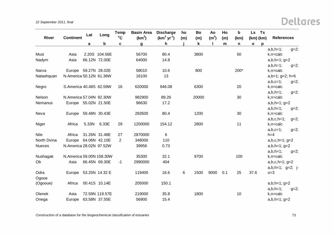
22 September 2011, final
Construction of a database for the biogeochemical classification of estuaries
73
Temp Basin Area Discharge ho Bo Ao Ho b Ls Ts Lat Long oC (km2) (km3 yr-1) (m) (m) (m2) (m) (km) (km) (km) River Continent a b c g h j k l m n o p
References
Musi Asia 2.20S 104.56E 56700 80.4 3800 50 a,b,h=1; g=2; k,n=calc
Nadym Asia 66.12N 72.00E 64000 14.8 a,b,h=1; g=2
Narva Europe 59.27N 28.02E 58010 10.6 800 200* a,b,h=1; g=2; k,n=calc
Natashquan N.America 50.12N 61.36W 16100 13 a,b=1; g=2; h=6
Negro S.America 40.48S 62.59W 16 620000 946.08 6300 20 a,b,c=1; g=2; k,n=calc
Nelson N.America 57.04N 92.30W 982900 89.26 20000 30 a,b,h=1; g=2; k,n=calc
Nemanus Europe 55.02N 21.50E 96630 17.2 a,b,h=1; g=2
Neva Europe 59.48N 30.43E 283500 80.4 1200 30 a,b,h=1; g=2; k,n=calc
Niger Africa 5.33N 6.33E 29 1200000 154.12 2800 11 a,b,c,h=1; g=2; k,n=calc
Nile Africa 31.26N 31.48E 27 2870000 6 a,b,c=1; g=2; h=4
North Dvina Europe 64.06N 42.10E 2 348000 110 a,b,c,h=1; g=2 Nueces N.America 28.02N 97.52W 39956 0.73 a,b,h=1; g=2
Nushagak N.America 59.00N 158.30W 35300 32.1 9700 100 a,b,h=1; g=2; k,n=calc
Ob Asia 66.45N 69.30E -1 2990000 404 a,b,c,h=1; g=2
Odra Europe 53.25N 14.32 E 119400 16.6 6 1500 9000 0.1 25 37.6 a,b,h=1; g=2; j-o=3
Ogooe (Ogooue) Africa 00.41S 10.14E 205000 150.1 a,b,h=1; g=2
Olenek Asia 72.59N 119.57E 219000 35.8 1800 10 a,b,h=1; g=2; k,n=calc
Onega Europe 63.58N 37.55E 56900 15.4 a,b,h=1; g=2

74
22 September 2011, final
Construction of a database for the biogeochemical classification of estuaries
Temp Basin Area Discharge ho Bo Ao Ho b Ls Ts Lat Long oC (km2) (km3 yr-1) (m) (m) (m2) (m) (km) (km) (km) River Continent a b c g h j k l m n o p
References
Orange Africa 28.41S 16.28E 16 1000000 11.36 700 20* a,b,c,h=1; g=2; k,n=calc
Orinoco S.America 8.37N 62.15W 24 1100000 1135 a,b,c,h=1; g=2
Panuco N.America
(MX) 21.59N 98.34W 66300 17.3 300 100* a,b,h=1; g=2; k,n=calc
Paraguay River S.America 19S 57W 363500 a,b=8; g=2 Paraibado Sul S.America 21.45S 41.20W 62760 30.6 a,b,h=1; g=2
Parana S.America 34.00S 58.17W 21 2783000 568 11300 50* a,b,c,h=1; g=2; k,n=calc
Pechora Europe 67.12N 52.03E 324000 131 8100 300* a,b,h=1; g=2; k,n=calc
Pee Dee N.America 34.12N 79.33W 22870 8.2 2200 8 a,b,h=1; g=2; k,n=calc
Peel N.America 67.37N 134.40W 71000 24.5 a,b,h=1; g=2
Penzhina Asia 62.28N 165.18E 85540 22.8 8200 25 a,b,h=1; g=2; k,n=calc
Petit (Mecatina) N.America 50.52N 59.36W 19600 16.2 a,b,h=1; g=2
Po Europe 44.53N 11.39E 13 70000 47.8 2 2100 4200 0.8 26 9.46 a,b,c=1; g=2; h=4; j-o=3
Potomac N.America 38.58N 77.09W 12.5 30000 9.654 6/5.13 230
a,b,h=1; c=33; g=2; j=28,33; n=30
Pungue (Pungoe) Africa 19.50S 34.48E 29000 3.1 4.3 6512 28000 6 20/34 70 120
a,b,h=1; g=2; k-m=7; o,p=26; j=29; n=7,30
Purari Oceania 7.25S 145.05E 33670 84.13 28300 18 a,b,h=1; g=2; k,n=calc

22 September 2011, final
Construction of a database for the biogeochemical classification of estuaries
75
Temp Basin Area Discharge ho Bo Ao Ho b Ls Ts Lat Long oC (km2) (km3 yr-1) (m) (m) (m2) (m) (km) (km) (km) River Continent a b c g h j k l m n o p
References
Rhine Europe 51.52N 6.02E 7.3 224000 69.4 15000 2-3 30
a,b,c=1; g=2,5; h=1,5; m=5; k,n=calc
Rhone Europe 43.55N 4.4E 13 95600 53.9 7 1000 7000 0.3 36 26 a,b,c=1; g=2; h=4 ; j-o=3
Rio Coatzacoalcos N.America 29497 a,b=1; g=2 Rio Grande (US) N.America 25.50N 97.31W 456700 0.72 a,b,h=1; g=2
Roanoake N.America 36.28N 77.38W 22458 7 22200 30 a,b,h=1; g=2; k,n=calc
Rufiji Africa 7.48S 37.55E 21 186100 35.2 2300 30 a,b,c,h=1; g=2; k,n=calc
Sabine N.America 30.18N 93.45W 23.4 18982 4.24 2.49 a,b,h=1; g=2; c,j=33
Sacramento N.America 38.35N 121.30W 60870 20.5 a,b,h=1; g=2
Sado Europe 38.5N -8.9E 22.9 7600 1.73448 1 2600 2600
2.9/ 1-
4/2.7 20 17.6 c=44; g=5; i=3,5 ; j-o=3; m=3,5,34
Saint John N.America 45.58N 67.14W 52850 35.6 a,b,h=1; g=2 Sakarya Asia 40.45N 30.23E 56830 5.87 a,b,h=1; g=2 Saloum Africa 3000 20000 k,l=7 San Joaquin N.America 37.41N 121.16W 35058 4 a,b,h=1; g=2 Sanaga Africa 3.36N 10.04E 119300 55 a,b,h=1; g=2
Savannah N.America 32.32N 81.16W 23.7 25511 10.6 3.08 3600 5.2* a,b,h=1; g=2; c,j=33; k,n=calc
Scheldt Europe 51.22N 4.15E 18.7 11400/21600 6 10 15000 150000 3.7/ 2-5 28 123 150
a,b=1; c=45; g=2,5; h=1,5; j-o=3; m=3,5; p=7
Sebou Africa 34.15N 6.40W 38492 63 a,b,h=1; g=2

76
22 September 2011, final
Construction of a database for the biogeochemical classification of estuaries
Temp Basin Area Discharge ho Bo Ao Ho b Ls Ts Lat Long oC (km2) (km3 yr-1) (m) (m) (m2) (m) (km) (km) (km) River Continent a b c g h j k l m n o p
References
Seine Europe 49.26N 00.26E 78600 15.8 6 13500 81000 7 9 44.2 a,b,h=1; g=2; j-o=3
Severn Europe 51.35N 2.40W 6800 2.58 10 19500 195000 12.3 25/20 118 a,b,g,h=1; j-o=3; n=3,30
Seyhan Europe 36.43N 34.53E 19300 4.8 200 3 a,b,h=1; g=2; k,n=calc
Skagit
N.America (in
Harrison, Europe!) 48.25N 122.20W 80000 14.6 a,b,g,h=1
Solimoes at Ica S.America 3S 70 W 1200000 1356.048 a,b=7; g=1
Solo Asia 6.47S 112.33E 16000 14.6 222 2070 0.5 226 a,b=1; g=2; h=6; k-n=7
St .Johns N.America 30.24N 81.24W 24.8 18373 16.12 2.21 3850 300* a,b=1; g=2; c,j=33; k,n=calc
St.Lawrence N.America 46.50N 71.15W 4 1020000 337 7/70 25 a,b,c,h=1; g=2; j=28,30; n=30
Stikine N.America 56.28N 132.23W 51593 50 12100 50 a,b,h=1; g=2; k,n=calc
Susitna N.America 61.16N 150.30W -1 50246 45.5 12500 18 a,b,c,h=1; g=2; k,n=calc
Susquehanna N.America 40.15N 76.52W 70189 34 2300 100 a,b,h=1; g=2; k,n=calc
Swan Canning Australia 38.23S 144.70E 126021 6 4110 a,b=1; g=2; k=31; j=46
Tamar Europe 50.4N -4.2E 1750 1.387584 10/2.9 4800 48000 4.7 7/25.5 46.4
a,b=6, k-m,o=3;g=27; j,n=3,30

22 September 2011, final
Construction of a database for the biogeochemical classification of estuaries
77
Temp Basin Area Discharge ho Bo Ao Ho b Ls Ts Lat Long oC (km2) (km3 yr-1) (m) (m) (m2) (m) (km) (km) (km) River Continent a b c g h j k l m n o p
References
Tana
Africa (not Tana in Norway) 2.32S 40.31E 42000 4.75 a,b,h=1; g=2
Tees Europe 76200 0.53 18/7.5 700 12600 4.4 17/217 84.5 a,b,h=1; g=2; k-m,o=3; j,n=3,30
Tejo Europe 38.44N 9.08W 73090 7 5800 40600 3.4 11 47 a,b,h=1; g=2; j-o=3
Tha Chin Asia 13.5N 100.3E 5.3 3600 3000 2.6 87/50 70 120
a,b,k-n=7;o,p=26;j=29; n=30
Thames Europe 51.28N 0.43E 16.98 15000/14000 3.17 8 7500 60000 6.5 / 3-6 23/42 86.8 110
a,b,h=1; c=47; g=1,5; j-l,o=3; m=3,5; p=26; n=3,30
Tiber (Tevere) Europe 41.54N 12.29E 16500 7.38 4 400 1600 0.8 19 20.1 a,b,g=1; h=4; j-o=3
Tocantins S.America 2.12S 49.30W 757000 372 66500 200 a,b=1; g=2; k,n=calc
Tornionjoki Europe 65.48N 24.08E 34510 11.86 2300 100* a,b,h=1; g=2; k,n=calc
Trinity N.America 30.26N 94.51W 47380 a,b=1; g=2 Trombetas S.America 0N 58W 130000 59.9184 a,b=8; g=2 Tugela Africa 30112 a,b=1; g=2 Tweed Europe 55.75N 2W 1500 2.459808 3 150 450 4.1 14 14.6 a,b=1; j-o=3 Tyne Europe 2200 0.094608 12 1200 14400 4.3 19 103 j-o=3; g=6 Ubangi Africa 356000 228 a,b,h=1; g=2 Uruguay S.America 33.55S 58.22W 240000 145 a,b,h=1; g=2
Usumacinta N.America
(MX) 17.25N 91.30W 67890 55.52 700 10 a,b,h=1; g=2; k,n=calc
Volga Europe 1350000

78
22 September 2011, final
Construction of a database for the biogeochemical classification of estuaries
Temp Basin Area Discharge ho Bo Ao Ho b Ls Ts Lat Long oC (km2) (km3 yr-1) (m) (m) (m2) (m) (km) (km) (km) River Continent a b c g h j k l m n o p
References
(Russia)
Waikato Oceania 37.17S 175.04E 13700 12.1 3000 100* a,b,h=1; g=2; k,n=calc
Weser Europe 53.32N 8.34E 45800 10.6 10 12000 120000 3.6 17 78.8 a,b,h=1; g=2; j-o=1
Wisla Europe 54.06N 18.47E 180000 32.5 4 2000 8000 0.1 23 25.3 a,b,h=1; g=2; j-o=3
Xijiang Asia 409000 270 a,b,h=1; g=2
Yana Asia 71.31N 136.32E -15 224200 34.3 6200 40 a,b,c,h=1; g=2; k,n=calc
Yenisei Asia 71.50N 82.40E -7 2590000 620 126300 150 a,b,c,h=1; g=2; k,n=calc
Yesil Asia
(Turkey) 41.24N 36.35E 35960 5.67 a,b,h=1; g=2
Yukon N.America 62.39N 164.48W -4 831387 200 7000 100* a,b,c,h=1; g=2; k,n=calc
Zaire (Congo River) Africa 6.04S 12.24e 23.6 3698000 1200 22800 70
a,b,c,h=1; g=2; k,n=calc
Zhujiang (Pearl River) Asia 22.40N 113.05E 21 407100 363 7 7100 100*
a,b,c,h=1; g=2; j=36; k,n=calc
Note: List of symbols and references at the end of the matrices. Where: ho= water depth at the mouth Bo= width at the mouth Ao= cross sectional area at the mouth Ho= tidal range

22 September 2011, final
Construction of a database for the biogeochemical classification of estuaries
79
b= width convergence length Ls= salt intrusion length Ts= tidal intrusion length
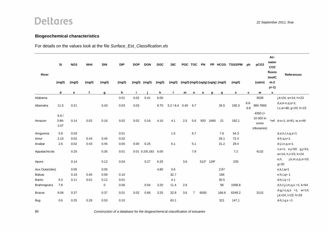
80
22 September 2011, final
Construction of a database for the biogeochemical classification of estuaries
Biogeochemical characteristics For details on the values look at the file Surface_Est_Classification.xls
Si NO3 NH4 DIN DIP DOP DON DOC DIC POC TOC PN PP HCO3- TSS/SPM ph pCO2
Air-water CO2
fluxes
(mg/l) (mg/l) (mg/l) (mg/l) (mg/l) (mg/l) (mg/l) (mg/l) (mg/l) (mg/l) (mg/l) (ug/g) (ug/g) (mg/l) (mg/l) (uatm) (molC m-2 yr-1)
River
d e f g h i j k l m n o p q s v w x
References
Alabama 0.01 0.02 0.41 6.00 3028 j,k=24; w=14; h=23
Altamaha 11.5 0.21 0.43 0.03 0.03 8.70 5.2 / 8.4 0.45 6.7 26.5 195.3 6.6-6.8
380-7800 d,e,k-n,q,s=1; l,v,w=48; g=20; h=23
Amazon 6.9 / 3.86- 2.07
0.14 0.02 0.16 0.02 0.02 0.16 4.10 4.1 2.5 5.6 920 1660 21 182.1
4350 (> 10 000 in
some tributaries)
*ref d-s=1; d=91; w,x=49
Amguema 5.9 0.03 0.01 1.5 6.7 7.6 54.3 d,e,h,l,n,q,s=1
Amur 2.15 0.02 0.43 0.45 0.02 29.1 72.4 d-h,q,s=1
Anabar 2.6 0.02 0.43 0.45 0.00 0.00 0.25 6.1 5.1 31.2 29.4 d-j,l,n,q,s=1
Appalachicola 0.25 0.35 0.01 0.01 0.2/0.183 6.00 7.9 7.2 4132 n,s=1; e,j=50; g,j=51; w=14; h,i=23; k=24
Apure 0.14 0.12 0.04 0.27 6.20 3.6 512* 128* 235 e,h, j,k,m,o,p,s=10; g=20
Aux Outar(des) 0.05 0.05 4.80 0.6 2.87 e,k,l,q=1
Balsas 0.19 0.40 0.59 0.10 32.7 166 e-h,l,q= 1
Barito 9.3 0.11 0.01 0.12 0.01 4.1 30.5 d-h,l,q =1
Brahmaputra 7.8 0 0.06 0.04 3.20 11.4 2.6 58 1058.8 d,h,f,j,l,m,q,s =1; k=64
Brazos 9.06 0.37 0.37 0.01 0.02 0.66 3.25 32.8 3.6 7 6500 166.6 6349.2 3115 d-g,l-o,q,s =1; w=14; j,k=24; i=23; h=33
Bug 0.6 0.25 0.28 0.53 0.10 63.1 321 147.1 d-h,l,q,s =1

22 September 2011, final
Construction of a database for the biogeochemical classification of estuaries
81
Si NO3 NH4 DIN DIP DOP DON DOC DIC POC TOC PN PP HCO3- TSS/SPM ph pCO2
Air-water CO2
fluxes
(mg/l) (mg/l) (mg/l) (mg/l) (mg/l) (mg/l) (mg/l) (mg/l) (mg/l) (mg/l) (mg/l) (ug/g) (ug/g) (mg/l) (mg/l) (uatm) (molC m-2 yr-1)
River
d e f g h i j k l m n o p q s v w x
References
Caroni 0.09 0.12 0.00 0.14 5.40 0.4 44* 5.6* 5 2957 e,h, j,k,m,o,p,s=10; w=14; g=20
Casamance 0.42 2.4-2.6 26.4 8.4 7.5 f,k,l,m,v=35
Caura 0.07 0.12 0.00 0.17 4.5 1 127* 9.9* 12 e,h, j,k,m,o,p,s=10; g=20
Cauweri 15.3 0.00 0.10 34.8 125 1.9 d,h,l,q,s =1
Chang Jiang (Yangtze)
6.5 0.32 0.32 0.64 0.02 2.1 27.7 1200 100 517 650-1440 15.5-34.2
d-h,k,l,q,s=1; l=52; l,w,x=53; k=24
Chao Phrya 15.8 0.14 0.1 0.24 0.03 15 76 395.7 d-h,l,q,s =1
Churchill (Hudson Bay)
1.4 0.01 0.01 0.02 0.01 12.1 8.8 32 d-h,l,n,q =1
Colorado (Ari) 8.75 0.35 0.35 0.10 0.02 0.56 7.1 40.4 3.3 540 135 6487 d,e,h,l,n,p-s=1; j,k=24; i=23
Colorado (Texas)
10.1 0.52 0.52 0.03 0.83 5.2 38.6 4.6 196.2 763.1 d,e,l,n,q,s=1; j,k=24; i=23
Columbia 9 /
3.25-0.69
0.2 0.01 0.21 0.01 0.01 2.7 0.26 2.34 63 63.6 6.63-8.68
560-950 d-h,l,q,s=1; d=91; w=13; m,n=54; v=55; i=23; k=24
Colville 0 1.21 7.6 10.5 53.5 317.5 l,q,s=1; j,k=24
Connecticut 5.06 / 3.36-0.87
0.03 0.03 0.02 0.25 3.8 5 7.1 25.6 d,l,n,q=1; d=91; j,k=24; h,i=23; e=33
Copper 0.41 0.02 0.28 6.3 1236.7 n,s=1; g=20; i=23; j=24
Corantijn 23.4 s=1
Dalalven 4.8 0.13 0.01 0.14 0.00 1.6 9.41 d-h,l,q=1
Danube 4.14 / 1.8 1.80 0.18 0.035 0.6 5.5 39.9 3.4 790 203 335 d,e,h-m,p-s=1; d=91

82
22 September 2011, final
Construction of a database for the biogeochemical classification of estuaries
Si NO3 NH4 DIN DIP DOP DON DOC DIC POC TOC PN PP HCO3- TSS/SPM ph pCO2
Air-water CO2
fluxes
(mg/l) (mg/l) (mg/l) (mg/l) (mg/l) (mg/l) (mg/l) (mg/l) (mg/l) (mg/l) (mg/l) (ug/g) (ug/g) (mg/l) (mg/l) (uatm) (molC m-2 yr-1)
River
d e f g h i j k l m n o p q s v w x
References
1.54-0.51
Daugava 2.8 0.19/0.98 0.1 1.08 0.04 26 13.1 132.4 23.4 d,e,h,l,n,q,s=1;e,f,g=56
Delaware 3.5 1 0.03 1.03 0.04/0.08 2.8 8.8 3 3100 39 39.3 2172 d-h,k,l,n,q,s=1; h,p=57; w=14
Dnepr 3.4 0.21 0.21 0.04 4.9 30 0.9 5.8 152.6 42.9 d,e,h,k-n,q,s=1
Dnestr 4.1 1 1 0.06 44.7 4.8 227.2 233.6 d,e,h,l,n,q,s=1
Don 0.28/4.8 0.23 0.08 0.31/ 3.7 0.042/ 0.13 4.2 39.4 1.7 5.9 201 76.9 7.56 *ref d-h,k-n,q,s=1; d,g,h=58; v,w=59
Douro 2 / 0.8-
1.12 0.05-1.3
0.003-0.11
0.0503-1.41
0.02-0.04 2.41 28.7 0.5 146 4/3.22 7.76 1330–2200
76 d,l,q=1; m,s,w=5; x=21, e-g=9; d,h=60; k,s,v=38
Drammenselva 0.28 0.02 0.30 0.00 2.9 177.7 e-h,n,s=1
Ebro 2.55 2.32 0.17 2.49 0.03 25.9 145 989 d,h,l,q,s=1; e-g=4
Eems 5.39 0.33 5.72 / 8.4 0.285 / 0.1 0.03 1.4 / 0.7 2.8 37 560–3755 67.3 e-h=1; m,s,w=5, x=21; g-j=61
Elbe 4.40 3.60 1.30 4.90 0.39 4 26 2.8 20.42 132 35.4/
43/15.03 8.01 580–1100 53
e-h,k,l,q,s=1; m,s,w=5; x=21; d,n,s=39; v=90
Evros 1.90 0.05 1.95 0.28 33.4 170 e-h=4; l,q=1
Fraser 5.46 0.10 0.10 0.05 3.7 10.1 6.3 51.3 175.4 7.84 d,e,h,k,l,n,q,s=1; v=62
Fuchun Jiang 4.72 1.43 0.03 1.46 0.05 1340 d-h,s=1
Gambia 10.8 0.00 0.02 2.28 4.5 1 2850 985 23 40.8 / 19.5 2072 d,h,k-m,o-s=1; w=14; s=16
Ganges 11.7 0.00 0.08 0.06 4.6 23.4 3.5 1150 500 88 1055 d,h,j-m,o-s=1
Garonne 4 0.23 2.43 0.10 26.2 1300 133 127.9 1675 d-h,l,p-s=1; w=14

22 September 2011, final
Construction of a database for the biogeochemical classification of estuaries
83
Si NO3 NH4 DIN DIP DOP DON DOC DIC POC TOC PN PP HCO3- TSS/SPM ph pCO2
Air-water CO2
fluxes
(mg/l) (mg/l) (mg/l) (mg/l) (mg/l) (mg/l) (mg/l) (mg/l) (mg/l) (mg/l) (mg/l) (ug/g) (ug/g) (mg/l) (mg/l) (uatm) (molC m-2 yr-1)
River
d e f g h i j k l m n o p q s v w x
References
Gironde 2.8-5 2-2.1 0.025-0.1 2.025-2.3 0.02-0.16 1.71 29.14 2.6 86/
650/1131.47 7.68 465–2860 30.8
m,s,w=5, x=21; d-h,s=92; k,l,s,v=40
Glama 0.42 0.04 0.46 0.01 2.6 4.17 13 665.2 h,l,n,q,s=1
Godavari 21.1 0.16 0.16 2 20.7/27 1-1.3 94 1619 8.75 293-500 *ref d,e,l,q,s=1; k,l,m,w =63; x=64
Grijalva 0.68 0.07 0.75 0.09 25.4 129 e-h,l,q=1
Guadiana 1.18 0.01 1.19 0.06 26 132 e-h,l,q=1
Gualdalquivir 15 0.00 36-59 233 7.8 1029-3605
d,q=1; l,v,w=65
Guaviare 0.05 0.07 4.8 2.9 31* 118 e,k,m,p,s=10; g=20
Huang He 9.5 2.20 0.01 2.21 0.02 1.75/2-
4 40.3 / 28-
29 132 1000 1100 163 26829 1137
d-h,k-s=1; k,l=52; w=14
Hudson 4.2 0.67 0.09 0.76 0.02 0.013 6.2 12.9 5 44 51 1125 / 1062
5.84-13
d-h,l,n,q,s=1; w,x=66; w=13; i=23; k=24
Humber 8.40 0.42 8.82 0.12 e,f,h=42
Hunter 0.00 0.06 h=23
Incomati 0.00
Indigirka 2.8 0.02 0.04 0.06 0.01 0.009 0.35 5.6 7.7 28.4 240.7 d-j,l,n,q,s=1
Indus 14 2.00 0.20 2.20 0.52 8.5 17.6 2.2 900 110 349 1748 d-h,l,m,p,q=1; w=14; s=18; k=24
Japura 0.10 0.11 0.01 0.204 3.4 1.7 122* 47* 55 e,h, j,k,m,o,p,s=10; g=20
Jurua 0.20 0.20 0.02 0.134 4.1 1.7 160* 146* 194 e,h, j,k,m,o,p,s=10; g=20
Kamchatka 12.6 0.10 0.05 0.15 0.08 9.6 48.6 81.6 d-h,l,q,s=1
Khatanga 3.2 0.03 0.04 0.07 0.01 0.006 0.41 9.4 6.3 47.9 16.8 d-j,l,n,q,s=1

84
22 September 2011, final
Construction of a database for the biogeochemical classification of estuaries
Si NO3 NH4 DIN DIP DOP DON DOC DIC POC TOC PN PP HCO3- TSS/SPM ph pCO2
Air-water CO2
fluxes
(mg/l) (mg/l) (mg/l) (mg/l) (mg/l) (mg/l) (mg/l) (mg/l) (mg/l) (mg/l) (mg/l) (ug/g) (ug/g) (mg/l) (mg/l) (uatm) (molC m-2 yr-1)
River
d e f g h i j k l m n o p q s v w x
References
Klamath 18 0.14 0.14 0.03 0.014 0.31 4.1 18.1 2.4 91.8 148.1 d,e,k,l,n,q,s=1; j=24; h,i=23
Kobuk 3.4 0.02 0.25 0.269 8.2 6.4 5.4 32.7 d,f,h,l,n,q=1; j=16; k=24
Kolyma 4 0.03 0.05 0.08 0.01 0.015 0.35 6.8 8.1 26 125.8 716-1779 d-j,l,n,q,s=1;w=67
Kuban 2.6 1.07 0.36 1.43 0.03 1.9 39.7 2.8 4.7 156.6 566.2 d-h,k-n,q,s=1
Kuskowin 7.6 0.27 0.026 0.74 4.6 17.6 4.1 89.6 116.9 d,k,l,n,q,s=1; g=20; i=23; j=24
Kymjoki 2.25 0.01 0.01 0.01 1.6 9.5 8 15.5 d,f,h,l,n,q,s=1
Lalang 0.00
Lena 4.2 / 2.01- 0.22
0.04 0.04 0.08 0.01 0.022 0.46 6.6 10.4 1.1 7.7 52 33 d-n,q,s=1; d=91
Liao 1.75 0.11 0.18 0.28 0.05 2531 d-h,s=1
Limpopo 17.7 0.00 28.3 144 1269 d,l,q,s=1
Loire 8 1.70 1.70 0.09 5.3 23.6/26.4-
32.4
2.7/ 2.9 / 2.7
8.1 120 37 / 35.5 8.3 630-2910 64.4 d,e,h,k,l,m,q=1; m,s=5; w,x=21; m,n,s=68; l,w=69; v=43
Luan 4.7 0.94 0.01 4762 d,e,h,s=1
Maas (Meuse)
6.85 2.78 0.23 6 68.6 d,e,h,n,s=1
MacKenzie 4 0.10 0.01 0.1 4.5 21.6 7.2 /3.2
12.5 / 22.6
2000 94 134.4 4663 d,e,h,j,k,l,m,n,o,q,s=1; w=14; m,n=18
Madeira 0.18 0.18 0.02 0.175 2.9 2.7 274* 304* 540 e,h, j,k,m,o,p,s=10; g=20

22 September 2011, final
Construction of a database for the biogeochemical classification of estuaries
85
Si NO3 NH4 DIN DIP DOP DON DOC DIC POC TOC PN PP HCO3- TSS/SPM ph pCO2
Air-water CO2
fluxes
(mg/l) (mg/l) (mg/l) (mg/l) (mg/l) (mg/l) (mg/l) (mg/l) (mg/l) (mg/l) (mg/l) (ug/g) (ug/g) (mg/l) (mg/l) (uatm) (molC m-2 yr-1)
River
d e f g h i j k l m n o p q s v w x
References
Mae Klong 0.00 627.9 s=1
Magdalena 12.6 0.22 0.22 0.12 9.7 49.3 928.3 d,e,h,l,q,s=1
Mahanadi 9 0.00 0.04 12 60.9 909.1 d,l,q,s=1; h=23
Manicoagan 0.03 0.03 5.2 0.7 3.48 e,k,l,q=1
Maputo 0.00
Mekong 8.9 / 0.14-1.4
0.00 11.4 2000 57.9 321.2 280-4110 d,l,p,q,s=1; d,w=70
Meta 0.11 0.13 0.204 3.1 7 75* 362 e,j,k,n,p,s=10; g=20
Mezen 2.4 0.01 0.06 0.07 0.03 12.3 62.3 32.5 d-h,l,q,s=1
Mississippi 6.7 / 2.74- 0.39
1.4 / 0.56 0.04 / 0.03 1.44 0.07 / 0.25 0.015 0.82 8/4.2 23.7 1.9 5.5 2800 98.5 862.1 7.98 2000,
4593/4752
d-h,k,l-o,q,s=1; e,f,h=71; d=91; v,w=72; w=14; k=15; j=24; i=23
Moise (Moisie)
3 0.06 0.06 4.4 1.6 8.29 d,e,k,l,q=1
Moose 0.00 20 17.2 0.8 87.5 8.8 k,l,m,q,s=1
Murray 5 0.11 0.04 0.15 0.02 19.5 9 69 1271.2 d-h,l,n,q,s=1
Musi 24.5 0.16 0.05 0.21 0.03 3 17 d-h,l,q=1
Nadym 9.3 0.14 0.83 0.15 5 20.8 d,e,n,s=1; h=23; f=73
Narva 0.40 g=20
Natashquan 0.00 5 0.7 3.48 k,l,q=1
Negro 16.3 0.04 0.04 0.00 0.155 8.5 13.9 0.4 8.36 1* 9* 70.8 454.2 d,l,q,s=1; e,h, j,k,m,o,p=10; n=11; g=20
Nelson 1.4 0.01 0.01 0.00 8 25.4 9 129 d,e,h,k,l,n,q=1

86
22 September 2011, final
Construction of a database for the biogeochemical classification of estuaries
Si NO3 NH4 DIN DIP DOP DON DOC DIC POC TOC PN PP HCO3- TSS/SPM ph pCO2
Air-water CO2
fluxes
(mg/l) (mg/l) (mg/l) (mg/l) (mg/l) (mg/l) (mg/l) (mg/l) (mg/l) (mg/l) (mg/l) (ug/g) (ug/g) (mg/l) (mg/l) (uatm) (molC m-2 yr-1)
River
d e f g h i j k l m n o p q s v w x
References
Nemanus 2.06 0.37 0.42 0.79 0.05 48.9 7.1 248.6 33.7 d-h,l,n,q,s=1
Neva 0.1 0.23 0.03 0.26 0.03 5.3 8.6 26.8 10.4 d-h,l,n,q,s=1
Niger 14 /
14.61 0.10 0.01 0.11 0.01 0.13
2.9 / 3.54
6.6 3.9 5.88 1600 33.5 259.5 /127 35617 d,j-l,o,q,s=1; e-h=11; w=14; d,k,m,n,s=16
Nile 12.8 3.00 3.00 0.01 3.5 34.2 4.4 900 135 1442 / 54 d,j-m,o,q,s=1; e=4; s=16
North Dvina 2.28 0.02 0.12 0.14 0.04 20.1 16.3 3.2 23.4 83 42.9 d-h,k-n,q,s=1
Nueces 13.4 2.04 2.04 0.04 0.75 7.2 39.9 21.2 202.8 710 d,e,l,n,q=1; s=6; j,k=24; i=23
Nushagak 0.12 0.011 0.44 3.2 g=20; i=23; j,k=24
Ob 2.85 0.06 0.60 0.66 0.07 9.1 29.5 0.9 10 78 40.8 30-140 d-h,k,l,m,n,q,s=1; k=24; w=67
Odra 2.42 0.21 2.63 / 2.7 0.370 / 0.09 29.5 150 7.1 e-h,l,q,s=1; g,h=74
Ogooe (Ogooue) 0.00 8.4 2.4 k,m=1
Olenek 2.7 0.03 0.05 0.08 0.00 0.006 0.41 14.3 7.2 72.6 32 d-j,l,n,q,s=1
Onega 7.5 0.15 *ref 0.02 15.8 20.7 72.3 19 d,e,h,l,n,q,s=1; f=73
Orange 16.9 0.72 0.72 0.01 0.15 2.33 21 0.85 107 7834.5 / 57 d,e,j-m,q,s=1; h=11; s=16
Orinoco 6.3 0.08 0.04 0.12 0.01 0.01 0.16 4.4 2 2.5 6 2200 550 9.99 132.2 d-s=1
Panuco 0.92 0.05 0.97 0.02 35 178 e-h,l,q=1
Paraguay River 0.00 g=20
Paraibado Sul
0.31 0.04 0.35 0.01 2.8 14 e-h,l,q=1
Parana 17.1 0.17 0.05 0.22 0.05 0.08 6.1 8.3 7.95 2.95 1400 598 21 139.1 3139 d-h,j-q,s=1; w=14
Pechora 1.6 0.01 0.22 0.23 0.01 12.7 7.7 0.3 13 38.9 50.4 8.05 d-h,k-n,q,s=1; v=75

22 September 2011, final
Construction of a database for the biogeochemical classification of estuaries
87
Si NO3 NH4 DIN DIP DOP DON DOC DIC POC TOC PN PP HCO3- TSS/SPM ph pCO2
Air-water CO2
fluxes
(mg/l) (mg/l) (mg/l) (mg/l) (mg/l) (mg/l) (mg/l) (mg/l) (mg/l) (mg/l) (mg/l) (ug/g) (ug/g) (mg/l) (mg/l) (uatm) (molC m-2 yr-1)
River
d e f g h i j k l m n o p q s v w x
References
Pee Dee 10.8 0.42 0.42 0.018 0.26 1.13 4.2 0.5 11 21.1 23 d,e,k,l,m,n,q,s=1; j=24; i=23
Peel 0.00 0.01 25.6 130 h,l,q=1
Penzhina 5.41 0.03 0.05 0.08 0.02 3.1 15.7 41 d-h,l,q,s=1
Petit (Mecatina) 0.01 0.01 6 0.8 3.84 e,k,l,q=1
Po 4 2.19 0.26 2.45 0.08 0.01 0.32 2.4 35 4.7 6500 1400 178 330.4 e-h=4; d,i-l,n-q,s=1
Potomac 6 1.20 0.03 1.23 0.03 0.03 0.44 3.1 14.6 5 74 65.5 646-878 d-h,k,l,n,q,s=1; w=13; j=24; i=23
Pungue (Pungoe) 0.00
Purari 13.8 0.04 0.04 0.08 0.00 15.9 81 950.9 d-h,l,q,s=1
Rhine 6.08 3.94 0.94 4.88 0.36 5.36 31.1 3/ 0.8 7 158 49.1/ 15 7.8 545–1990 39.7 d-h,k-n,q,s=1; m,s,w=5, x=21; v=76
Rhone 3.0 / 1.37-0.66
1.48 0.12 1.60 0.10 34.6 176 517.5 2015 e-h=4; d,l,q,s=1; d=91; w=14
Rio Coatzacoalcos 0.00 0.87 j=24
Rio Grande (US)
14 0.15 0.03 0.18 0.03 0.016 0.57 4.1 31.4 7 130 1111.1 1205 d-h,l,n,q,s=1, w=14; j,k=24; i=23
Roanoake 0.00 0.018 0.22 7.1 285.7 n,s=1; j=24; i=23
Rufiji 1.30 0.10 1.40 0.01 9.8 50 483 e-h,l,q,s=1
Sabine 8 0.08 0.08 0.01 0.017 0.52 6 4.0 / 7.2 8.3 20.5 176.9 d,e,l,n,q,s=1; k,l =77; j=24; i=23; h=33
Sacramento 17 0.10 0.03 0.13 0.03 0.018 0.41 3.6 11.7 2 59.5 112.2 1955 d-h,k,l,n,q,s=1; w=14; j=24; i=23
Sado 5 0.84 0.07 0.91 0.06 6.72 28.21 2.9 101 / 80-
250 7.62 575–5700 31.1
m,s,w=5,x=21; d-h,s=92; k,l,v=44

88
22 September 2011, final
Construction of a database for the biogeochemical classification of estuaries
Si NO3 NH4 DIN DIP DOP DON DOC DIC POC TOC PN PP HCO3- TSS/SPM ph pCO2
Air-water CO2
fluxes
(mg/l) (mg/l) (mg/l) (mg/l) (mg/l) (mg/l) (mg/l) (mg/l) (mg/l) (mg/l) (mg/l) (ug/g) (ug/g) (mg/l) (mg/l) (uatm) (molC m-2 yr-1)
River
d e f g h i j k l m n o p q s v w x
References
Saint John 2.7 0.08 0.01 0.09 7.42 4.3 11.3 21.9 d-g,l,n,q=1; j=20
Sakarya 11.8 1.11 0.35 1.46 0.16 39.3 206 1499.1 d-h,l,q,s=1
Saloum 0.00
San Joaquin 15.75 0.81 0.81 0.027 0.44 8.8 24.4 5.2 124 19.4 d,e,l,n,q,s=1; j,k=24; i=23
Sanaga 15.5 0.00 3.5 4.1 3.2 20.85 50.9 d,k,l,m,q,s=1
Savannah 8.9 0.23 0.23 0.01 0.025 0.27 5.5 4.9 0.9 4.6 25 241.4 d,e,k,l,m,n,q,s=1; j=24; i=23; h=33
Scheldt 7 / 2.8-
7.3 4.6 / 3.5
/4.5 7.7 / 1.4 12.30
0.81/0.5/0.25/ 0.16
0.031 7.9/10.8 54.9 / 66 / 39.6-85.2
18.3 / 10.8
7.05 5580 279 166.7/163 7-7.5 125–9425
/5000 63
/240
e-h,k,l,n,q,s=1, m,s,w=5; x=21; d,e,h,v=78; e,f,g,k,l=79; h,i,p=80; l,w,x=45; d=81; l=82
Sebou 10.6 0.00 0.9 960 412.7 d,p,s=1; j=24
Seine 6.33 4.38 2.41 6.79 0.70 0.5 3.65 49.6 2.65 6.3 252 44.3 826-5345 d-h,j-n,q,s=1; w=13
Severn 0.00 0.02 170.5 s=1; h=23
Seyhan 0.59 0.31 0.90 0.01 31.2 158.5 1083.3 e-h,l,q,s=1
Skagit 0.00 0.01 2.8 22 n,s=1; h=23
Solimoes at Ica 0.21 0.12 g,j=20
Solo 19.6 0.28 0.28 0.03 24 122 1266.7 d,e,h,l,q,s=1
St .Johns 0.0042 0.01 0.012 0.44 12.6 13.7 n=1; i=23; j,k=24; e,h=33
St.Lawrence 2.4 0.16 0.08 0.24 0.05 0.021 0.03 3.7 17.1 0.8 4.5 820 88.1 11.7 *ref d-g,i-n,p-s=1; i,h=23; w=83
Stikine 6 0.09 0.24 0.02 0.017 0.84 3.6 12.8 2.4 48.7 396 d,k,l,n,q,s=1; e=11;
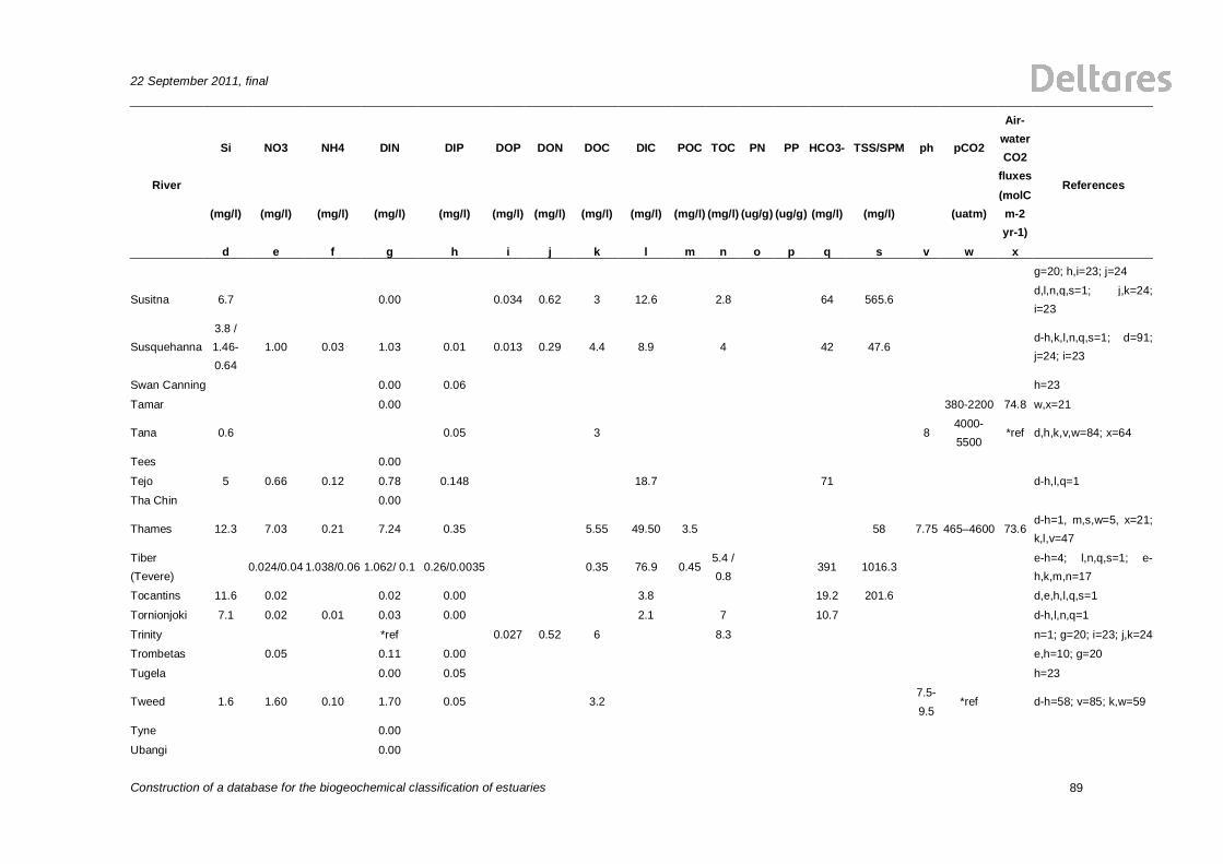
22 September 2011, final
Construction of a database for the biogeochemical classification of estuaries
89
Si NO3 NH4 DIN DIP DOP DON DOC DIC POC TOC PN PP HCO3- TSS/SPM ph pCO2
Air-water CO2
fluxes
(mg/l) (mg/l) (mg/l) (mg/l) (mg/l) (mg/l) (mg/l) (mg/l) (mg/l) (mg/l) (mg/l) (ug/g) (ug/g) (mg/l) (mg/l) (uatm) (molC m-2 yr-1)
River
d e f g h i j k l m n o p q s v w x
References
g=20; h,i=23; j=24
Susitna 6.7 0.00 0.034 0.62 3 12.6 2.8 64 565.6 d,l,n,q,s=1; j,k=24; i=23
Susquehanna 3.8 / 1.46-0.64
1.00 0.03 1.03 0.01 0.013 0.29 4.4 8.9 4 42 47.6 d-h,k,l,n,q,s=1; d=91; j=24; i=23
Swan Canning 0.00 0.06 h=23
Tamar 0.00 380-2200 74.8 w,x=21
Tana 0.6 0.05 3 8 4000-5500
*ref d,h,k,v,w=84; x=64
Tees 0.00
Tejo 5 0.66 0.12 0.78 0.148 18.7 71 d-h,l,q=1
Tha Chin 0.00
Thames 12.3 7.03 0.21 7.24 0.35 5.55 49.50 3.5 58 7.75 465–4600 73.6 d-h=1, m,s,w=5, x=21; k,l,v=47
Tiber (Tevere)
0.024/0.04 1.038/0.06 1.062/ 0.1 0.26/0.0035 0.35 76.9 0.45 5.4 / 0.8
391 1016.3 e-h=4; l,n,q,s=1; e-h,k,m,n=17
Tocantins 11.6 0.02 0.02 0.00 3.8 19.2 201.6 d,e,h,l,q,s=1
Tornionjoki 7.1 0.02 0.01 0.03 0.00 2.1 7 10.7 d-h,l,n,q=1
Trinity *ref 0.027 0.52 6 8.3 n=1; g=20; i=23; j,k=24
Trombetas 0.05 0.11 0.00 e,h=10; g=20
Tugela 0.00 0.05 h=23
Tweed 1.6 1.60 0.10 1.70 0.05 3.2 7.5-9.5
*ref d-h=58; v=85; k,w=59
Tyne 0.00
Ubangi 0.00

90
22 September 2011, final
Construction of a database for the biogeochemical classification of estuaries
Si NO3 NH4 DIN DIP DOP DON DOC DIC POC TOC PN PP HCO3- TSS/SPM ph pCO2
Air-water CO2
fluxes
(mg/l) (mg/l) (mg/l) (mg/l) (mg/l) (mg/l) (mg/l) (mg/l) (mg/l) (mg/l) (mg/l) (ug/g) (ug/g) (mg/l) (mg/l) (uatm) (molC m-2 yr-1)
River
d e f g h i j k l m n o p q s v w x
References
Uruguay 15 0.23 0.05 0.28 0.04 3.2 7.1 0.7 4 26 75.9 d-h,k-n,q,s=1
Usumacinta 0.44 0.05 0.48 0.09 27.7 141 e-h,l,q=1
Volga 0.00 0.01 h=11
Waikato 28.2 0.30 0.01 0.31 0.02 0.05 8.3 6.1 2300 35.3 132.2 d-h,j,l,n,p-s=1
Weser 4 5.08 0.13 5.21 0.37 33 168 26.11 4395 d-h,l,q,s=1; w=14
Wisla 1.83 0.44 2.27 0.21 37.4 190 73.3 d-h,l,q,s=1
Xijiang 0.00 600-7200 69-130
w,x=86
Yana 2.2 0.01 0.17 0.18 0.00 0.01 0.4 4.1 6.7 20.7 114.4 d-j,l,n,q,s=1
Yenisei 3 0.02 0.28 0.30 0.01 7.4 11.3 7.4 57.3 9.5 30-140 d-h,k,l,n,q,s=1; w=67
Yesil 0.53 0.27 0.80 0.08 3351 e-h,s=1
Yukon 6.9 /7.7 0.1/0.117 0.03/0.061 0.13/0.178 0.01/0.011 0.018 0.287 4.8 21.4 1.33 7 81/ 109
300 5205/2767 d-h,k-n,q,s=1; w=14; d-h,j=16; i=23
Zaire (Congo River)
9.4 / 5.2- 1.07
0.09 0.01 0.10 0.02 0.18 8.5 3.1 1 8.8 2060 15.7 19 d-h,j-m,p-s=1; d=91; n=11; s=16
Zhujiang (Pearl River)
8.5/ 3.5-4.0
0.62 0.01 0.63/1.05-
1.54 0.003/0.0062-
0.037 19.7 100 190.1
7.0-7.7
4000 d-h,l,q,s=1, l,v=87, d,g,h,l=88; w=89
* (columns: o & p) are in ug/l *ref = check reference

22 September 2011, final
Construction of a database for the biogeochemical classification of estuaries
1 of 90
References for the database: 1- Meybeck & Ragu, 1995 2- NEWS publications 3- GEMCO, 2003 4- UNEP/MAP, 2003 5- Abril et al 2002 6- Milliman et al 1995 (GLORI database) 7- Savenije, 1992 8- Lewis et al., 1999 9- Middelburg & Nieuwenhuize, 2000 10- Lewis et al., 1995 11- Meybeck 1982 13- Abril & Borges, 2004 14- Cole & Caraco, 2001 15- Dagg et al., 2004 16- Martins & Probst (SCOPE/UNEP Report 42) 17- SCOPE/UNEP Report 64 18- SCOPE/UNEP Report 58 20- Seitzinger & Harrison, 2008 21- Borges et al., 2006 23- Harrison et al_2005 24- Harrison et al_2005 (b) 26- Savenije, 2005 27- Williams et al, 2001 28-Lanzoni & Seminara (1998) 29- Savenije, 2001 30-Toffolon et al., 2006 31- OZ Coasts 32- CSIRO 33- NEEA Estuaries Database 35- Pages et al., 1995 36- Liu et al., 2009 37- The Estuary Guide, 2009 38- Frankignoulle et al., 2006 (a) 39- Frankignoulle et al., 2006 (b) 40- Frankignoulle et al., 2006 (c) 41- Uncles et al., 1998 42- Sanders et al., 1997 43- Frankignoulle et al., 2006 (d) 44- Frankignoulle et al., 2006 (e) 45- Frankignoulle et al., 2006 (f) 46- Robson et al., 2008 47- Frankignoulle et al., 2006 (g) 48- Cai & Wang, 1998 49- Richey et al., 2002 50- Mortazavi et al., 2001 51- Mortazavi et al., 2000 52- Cauwet & MacKenzie, 1993 53- Zhai et al., 2007

2 of 90
Construction of a database for the biogeochemical classification of estuaries
22 September 2011, final
54- Dahm et al., 1981 55- Park et al., 1970 56- Stalnacke et al., 2003 57- Lebo, 1991 58- Balls, 1994 59- Neal et al., 1998 60- Azevedo et al., 2008 61- Beusekom & de Jonge, 1998 62- De Mora S.J, 1983 63- Bouillon et al., 2003 64- Gupta et al., 2009 65- De la Paz et al., 2007 66- Raymond et al., 1997 67- Semiletov, 1999 68- Meybeck et al., 1988 69- Abril et al., 2003 70- Borges et al., 2005 71- Fox et al., 1987 72- Cai., 2003 73- Homes et al., 2002 74- Pastuszak et al., 2005 75- Nikiforov et al., 2008 76- Frankignoulle et al., 2006 (h) 77- Kaldy et al., 2005 78- Zwolsman, 1994 79- Soetaert et al., 2006 80- Van der Zee et al., 2007 81- Kronkamp et al., 1995 82- Hellings et al., 2001 83- Helie et al., 2002 84- Boullion et al., 2007 85- Howland et al., 2000 86- Yao et al., 2007 87- Guo et al., 2008 88- Cai et al., 2004 89- Zhai et al., 2005 90- Brasse et al., 2002 91- Conley, 1997 92- Cabecadas et al., 1999