construction, testing, and characterization of ... -...
TRANSCRIPT
Construction, Testing, and
Characterization of Vertical Drift
Chambers for Qweak
A thesis submitted in partial fulfillment of the requirementfor the degree of Bachelor of Science with Honors in
Physics from the College of William and Mary in Virginia,
by
Douglas C. Dean III
Accepted for Honors
Advisor: Prof. David S. Armstrong
Prof. Gina L. Hoatson
Prof. Todd D. Averett
Prof. Robert M. Lewis
Williamsburg, VirginiaMay 2009
Contents
Acknowledgments iii
List of Figures v
List of Tables vi
Abstract v
1 Introduction 1
2 The Qweak Experiment 3
2.1 Overview of Qweak . . . . . . . . . . . . . . . . . . . . . . . . . . . . 3
2.2 Physics of Qweak . . . . . . . . . . . . . . . . . . . . . . . . . . . . . . 4
2.2.1 Parity . . . . . . . . . . . . . . . . . . . . . . . . . . . . . . . 6
2.2.2 Asymmetry . . . . . . . . . . . . . . . . . . . . . . . . . . . . 7
2.3 Design of Qweak . . . . . . . . . . . . . . . . . . . . . . . . . . . . . . 7
2.4 Tracking System . . . . . . . . . . . . . . . . . . . . . . . . . . . . . 10
2.4.1 Drift Chambers . . . . . . . . . . . . . . . . . . . . . . . . . . 11
2.4.2 Vertical Drift Chambers . . . . . . . . . . . . . . . . . . . . . 13
3 Construction of Vertical Drift Chamber 16
4 Testing of the Vertical Drift Chamber 24
i

4.0.3 Overview . . . . . . . . . . . . . . . . . . . . . . . . . . . . . 24
4.0.4 Gas Handling System Testing . . . . . . . . . . . . . . . . . . 24
4.0.5 High Voltage Testing and Conditioning . . . . . . . . . . . . . 26
4.0.6 Chamber Efficiency Testing . . . . . . . . . . . . . . . . . . . 37
4.1 Conclusions and Future Plans . . . . . . . . . . . . . . . . . . . . . . 50
ii
Acknowledgments
I would like to thank Professor Armstrong his time and patience that he has
given me. This project would have been very difficult without his constant help.
Also, I would like to thank John Leckey for his explanations that helped me better
understand key concepts of this project.
iii
List of Figures
2.1 Running of sin2θW . . . . . . . . . . . . . . . . . . . . . . . . . . . . 5
2.2 Parity Transformation . . . . . . . . . . . . . . . . . . . . . . . . . . 6
2.3 Qweak Experimental Setup . . . . . . . . . . . . . . . . . . . . . . . . 8
2.4 Qweak Beamline Path through Setup . . . . . . . . . . . . . . . . . . . 9
2.5 Vertical Drift Chamber Mounting . . . . . . . . . . . . . . . . . . . . 11
2.6 Cross Section of Vertical Drift Chamber . . . . . . . . . . . . . . . . 14
2.7 Electric Field Lines of VDC . . . . . . . . . . . . . . . . . . . . . . . 15
3.1 Layers of VDC Chamber . . . . . . . . . . . . . . . . . . . . . . . . . 17
3.2 Layout of Chamber . . . . . . . . . . . . . . . . . . . . . . . . . . . . 17
3.3 Seperate Components of G10 Frame . . . . . . . . . . . . . . . . . . . 18
3.4 Completed G10 Frame . . . . . . . . . . . . . . . . . . . . . . . . . . 19
3.5 High Voltage Frame . . . . . . . . . . . . . . . . . . . . . . . . . . . . 19
3.6 Lab Table Used for Making G10 Frames . . . . . . . . . . . . . . . . 20
3.7 Tin Coated Copper Strips Around Outside of HV Frame . . . . . . . 21
3.8 Wire Frame . . . . . . . . . . . . . . . . . . . . . . . . . . . . . . . . 21
3.9 Sketch of the Gas Handling System Used for VDC . . . . . . . . . . . 22
3.10 Bubbler . . . . . . . . . . . . . . . . . . . . . . . . . . . . . . . . . . 23
4.1 Gas Handling System Connections . . . . . . . . . . . . . . . . . . . 27
4.2 Grounding Sense Wires for High Voltage Testing . . . . . . . . . . . . 28
iv
4.3 Plot of Initial Conditioning of Chamber . . . . . . . . . . . . . . . . . 31
4.4 Log Plot of Initial Conditioning of Chamber . . . . . . . . . . . . . . 32
4.5 Evidence of Arcing Within the Chamber . . . . . . . . . . . . . . . . 34
4.6 Garfield Simulation without Missing Wire . . . . . . . . . . . . . . . 35
4.7 Garfield Simulation with Missing Wire . . . . . . . . . . . . . . . . . 36
4.8 Different Current vs. Voltage Plots Made During Conditioning . . . . 37
4.9 Log Plot of Current vs. Voltage During Conditioning . . . . . . . . . 38
4.10 NIM Module Setup Used for Measuring Efficiency . . . . . . . . . . . 39
4.11 Plot of Initial Efficiency of Chamber . . . . . . . . . . . . . . . . . . 42
4.12 Logic Diagram for Electronics of Efficiency Testing . . . . . . . . . . 44
4.13 Timing Diagram for Electronics of Efficience Testing . . . . . . . . . 45
4.14 Efficiency Setup with MAD Card . . . . . . . . . . . . . . . . . . . . 46
4.15 Plot of Final Measurements of Efficiency . . . . . . . . . . . . . . . . 48
4.16 Copper Shielding Used on MAD card . . . . . . . . . . . . . . . . . . 49
4.17 Plot of Current Being Drawn From Indiviual Wire Cards . . . . . . . 51
v

List of Tables
4.1 Initial Conditioning of Chamber . . . . . . . . . . . . . . . . . . . . . 30
4.2 Conditioning of Chamber After Time . . . . . . . . . . . . . . . . . . 33
4.3 Initial Efficiency of Chamber using 90Sr Source Without 2nd Readout
Card . . . . . . . . . . . . . . . . . . . . . . . . . . . . . . . . . . . . 41
4.4 Initial Efficiency of Chamber using 90Sr Source With 2nd Readout Card 41
4.5 Efficency Testing with 90Sr Source . . . . . . . . . . . . . . . . . . . 47
4.6 Efficency Testing with Cosmic Rays . . . . . . . . . . . . . . . . . . . 47
vi

Abstract
Qweak is an experiment set to take place at Jefferson Lab that will put the
Standard Model to the test by measuring the weak charge of the proton by precisely
measuring the parity-violating asymmetry of elastic proton-electron scattering. Ver-
tical Drift Chambers, which will momentum analyze events that take place, will be
key to the tracking system of Qweak. A vertical drift chamber was constructed and
conditioned by applying high voltage to the chamber. After conditioning, the current
that the chamber would draw at 3.55kV began to spike to 10.3µA and therefore we
were cautious to go above this voltage level when testing the chamber. The efficiency
of the chamber was measured using cosmic rays and a 90Sr source. Using cosmic
rays, the efficiency of the chamber was (95.3 ± 1.3)% at 3.5kV, whereas when using
the 90Sr source, the efficiency of the chamber was (81.3 ± 1.9)% at 3.5kV. However,
it was discovered that these efficiencies were contaminated by background noise that
was being picked up by the electronic equipment used to measure the efficiency. After
eliminating this background noise, the efficiency of the chamber was again measured,
yet it was not at an operating efficiency, which is typically on the order of 99 - 100%.
It appeared that the chamber needed to be able to handle larger voltages, however,
this was not possible due to the amount of current that the chamber would draw at
these larger voltages. It was discovered that the bottom wire frame was the source
of the current at these large voltages, so we decided to disassemble the chamber and
replace this wire frame. The chamber was then reassembled and is currently being
conditioned.

Chapter 1
Introduction
The Standard Model of Particle Physics was developed in the 1970’s as a means
to connect the electromagnetic, strong and weak interactions, yet, the theory is viewed
as incomplete because it does not correctly account for the gravitational force. Al-
though the Standard Model has correctly predicted what has been observed by ex-
periments, there is reason to believe that the Standard Model is not “the” model for
particle physics. One of the major inconsistencies with the Standard Model is that
it contains many free parameters. Ideally, a unifying theory tries to minimize free
parameters, yet, the Standard Model contains as many as 17 free parameters. The
mysterious Higgs Boson, which is predicted by the Standard Model, has yet to be
discovered although many experiments have been designed to find it. (However, one
explanation why the Higgs may have not been discovered yet could be that the mass
of the Higgs is above the upper limit of mass for the designed experiments, preventing
the Higgs from being detected.) Experiments have also verified that the neutrino has
mass, which is inconsistent with the predictions of the Standard Model, which was
originally constructed with massless neutrinos. These inconsistencies have raised the
question whether there is a physics beyond the Standard Model, creating a need to
test the Standard Model. The Qweak experiment seeks to measure the weak charge of
the proton, which is firmly predicted by the Standard Model, and therefore will serve
1
as a test of the Standard Model.
The purpose of this research has been threefold. The first part of this project
has been to aid in the completion of a vertical drift chamber that will be used in
the Qweak experiment. Drift chambers, which are precision gas-filled wire chambers,
will be used in Qweak for the detection of elastically scattered electrons. Much work
on building a drift chamber, including the process of how the chamber will be built,
had been accomplished before the start of this project, yet, not all components of the
chamber had been finished. Also, a gas handling system to monitor the outflow and
leak rate of the gas used to pressurize the chamber was designed and built.
The two other components of the research project has consisted of testing the
completed drift chamber and analyzing the data collected. High voltage, which is
necessary for the operation of a drift chamber, was carefully applied to chamber using
a high voltage power supply. Once the chamber had been ”conditioned,” testing of
the efficiency of a single wire was started. For this, cosmic rays and a 90Sr radioactive
source was used.
2
Chapter 2
The Qweak Experiment
2.1 Overview of Qweak
The Qweak experiment will attempt to make an extremely precise measurement
of the weak charge of the proton as a means of testing the Standard Model. The weak
charge of the proton, QP
W, is a measure of the strength of the neutral weak coupling
of the proton, analogous to the electric charge for the electromagnetic interaction. In
the Standard Model, it is related to the weak mixing angle, θW , via
QP
W= 1 − 4sin2θW . (2.1)
The experiment will use Thomas Jefferson National Laboratory’s (JLab) leading
parity-violation facility to measure the parity-violating asymmetry in elastic proton-
electron scattering due to the weak interaction at a low momentum transfer. It is
required that the experiment be highly precise, with a combined statistical and sys-
tematical error of 4%.
The Standard Model predicts the weak charge of the proton based on the “run-
ning” of the weak mixing angle sin2θW . The weak mixing angle is a parameter in the
Standard Model that varies as a function of the momentum transfer at which it is
probed. In the Standard Model, the weak mixing angle is defined as the ratio of the
3
masses of the W± and Z0 bosons by
cos2θW =M2
W±
M2Z0
(2.2)
and connects the weak interaction to the electromagnetic interaction, i.e. the mixing
of these interactions. In any process that a photon can be exchanged, a Z0 can
also be exchanged [1]. At energies and momentum transfers larger than the mass
of the Z0, the Z0 exchange contributions are comparable to that of photons, and
therefore the process that takes place involves both the weak and electromagnetic
interactions. The mixing of these interactions is related to the parameter sin2θW .
Figure 2.1 illustrates both the Standard Model’s prediction of sin2θW as a function of
the momentum transfer, Q, and previous measurements of the “running” of sin2θW .
The first of these points, labeled APV , corresponds to an atomic parity violation
experiment using 137Cs [6, 9]. The second, Qw(e), corresponds to a measurement from
the parity violating Møller experiment [6, 10]. The third, ν−DIS, is a measurement
taken from the neutrino/antineutrino scattering from iron [6, 11]. Qweak differs from
these other measurements in that it will measure the “running” of sin2θW to a much
higher precision, which is indicated by the error bars in Figure 2.1. It is key to point
out when looking at Figure 2.1 that the measurements of the future experiments are
arbitrarily placed on the plot since it can not be sure what these measurements will
be.
2.2 Physics of Qweak
The asymmetry in parity-violating elastic proton-electron scattering that Qweak
will measure is a result of the weak interaction that takes place between the proton
and electron. The weak interaction, which is experienced by quarks and leptons, is
carried by three bosons, W+, W−, and the Z0, which all three act differently with
4
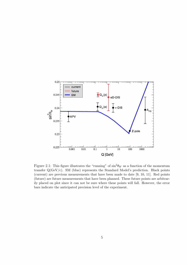
Figure 2.1: This figure illustrates the “running” of sin2θW as a function of the momentumtransfer Q(GeV/c). SM (blue) represents the Standard Model’s prediction. Black points(current) are previous measurements that have been made to date [9, 10, 11]. Red points(future) are future measurements that have been planned. These future points are arbitrar-ily placed on plot since it can not be sure where these points will fall. However, the errorbars indicate the anticipated precision level of the experiment.
5

Figure 2.2: This figure illustrates a parity operation acting upon a Cartesian CoordinateSystem. The parity operation inverts the spatial coordinates of the Cartesian CoordinateSystem. Notice that the system is transformed from a right handed system to a left handedsystem.
fermions [1]. Specifically, the W+ has a charge of +1 and only acts on a fermion that
has spin parallel to its velocity (right-handed fermions). The W− has a charge of
-1 and only acts on a fermion that has spin anti-parallel to its velocity (left-handed
fermions). The Z0 is neutral and acts on both right handed and left handed fermions,
however it acts on the two types with a different magnitude, creating an asymmetry
between the probability for scattering of right-handed and left-handed fermions.
2.2.1 Parity
A parity operation is a spatial inversion which inverts the coordinates of a vector
~r to −~r, and therefore a parity operation acting on a right-handed coordinate system
transforms the system into a left-handed coordinate system, as shown in Figure 2.2
[2, 3, 4]. It was originally believed that the laws of physics were invariant under a
parity operation, meaning that one could not tell the difference between right and
left-handed systems. However, in 1956, Lee and Yang predicted that parity might
be violated in weak interactions which was confirmed experimentally using the beta
decay of 60Co soon after by Wu et al. [2].
6
2.2.2 Asymmetry
The asymmetry that is created by the parity-violating elastic proton-electron
scattering is defined by
A ≡σ+ − σ+
σ+ + σ−, (2.3)
where σ+ is represents the the scattering cross section of the fermions that are right
handed and σ− represents the scattering cross section of the fermions that are left
handed. By applying Quantum Field Theory, one can also show that the asymmetry
is proportional to the weak charge of the proton [5], given by
A =1
P
−GF
4πα√
2[Q2QP
W+ Q4B(Q2)]. (2.4)
This equation is a low order approximation of the asymmetry, with P representing
the polarization of the electron beam, Q2 representing the 4-momentum transfer, GF
representing the Fermi coupling and α is the fine structure constant. Higher-order
terms, (arising from hadronic structure effects, such as gluons), are represented by
Q4B(Q2) and can be ignored at low momentum transfers. Thus, at a low momentum
transfer, by measuring the asymmetry in the elastic proton-electron scattering, the
measurement of the weak charge of the proton can be made, which is how Qweak will
measure the weak charge of the proton.
2.3 Design of Qweak
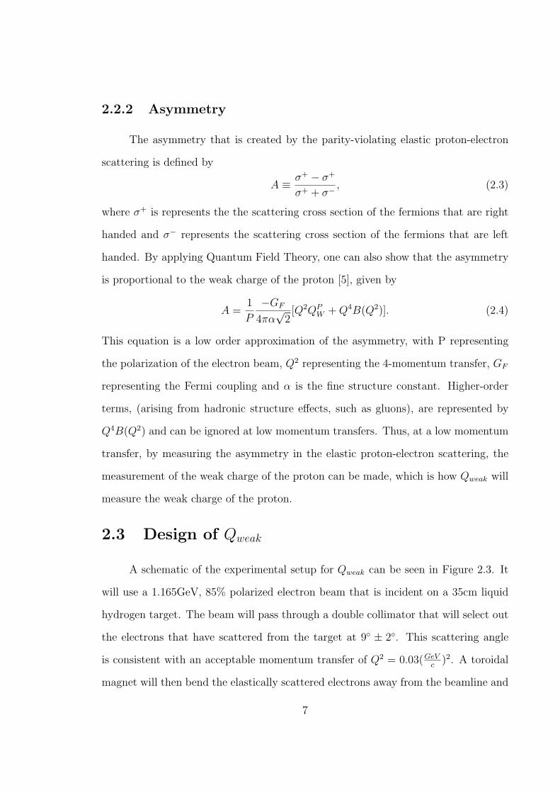
A schematic of the experimental setup for Qweak can be seen in Figure 2.3. It
will use a 1.165GeV, 85% polarized electron beam that is incident on a 35cm liquid
hydrogen target. The beam will pass through a double collimator that will select out
the electrons that have scattered from the target at 9 ± 2. This scattering angle
is consistent with an acceptable momentum transfer of Q2 = 0.03(GeV
c)2. A toroidal
magnet will then bend the elastically scattered electrons away from the beamline and
7
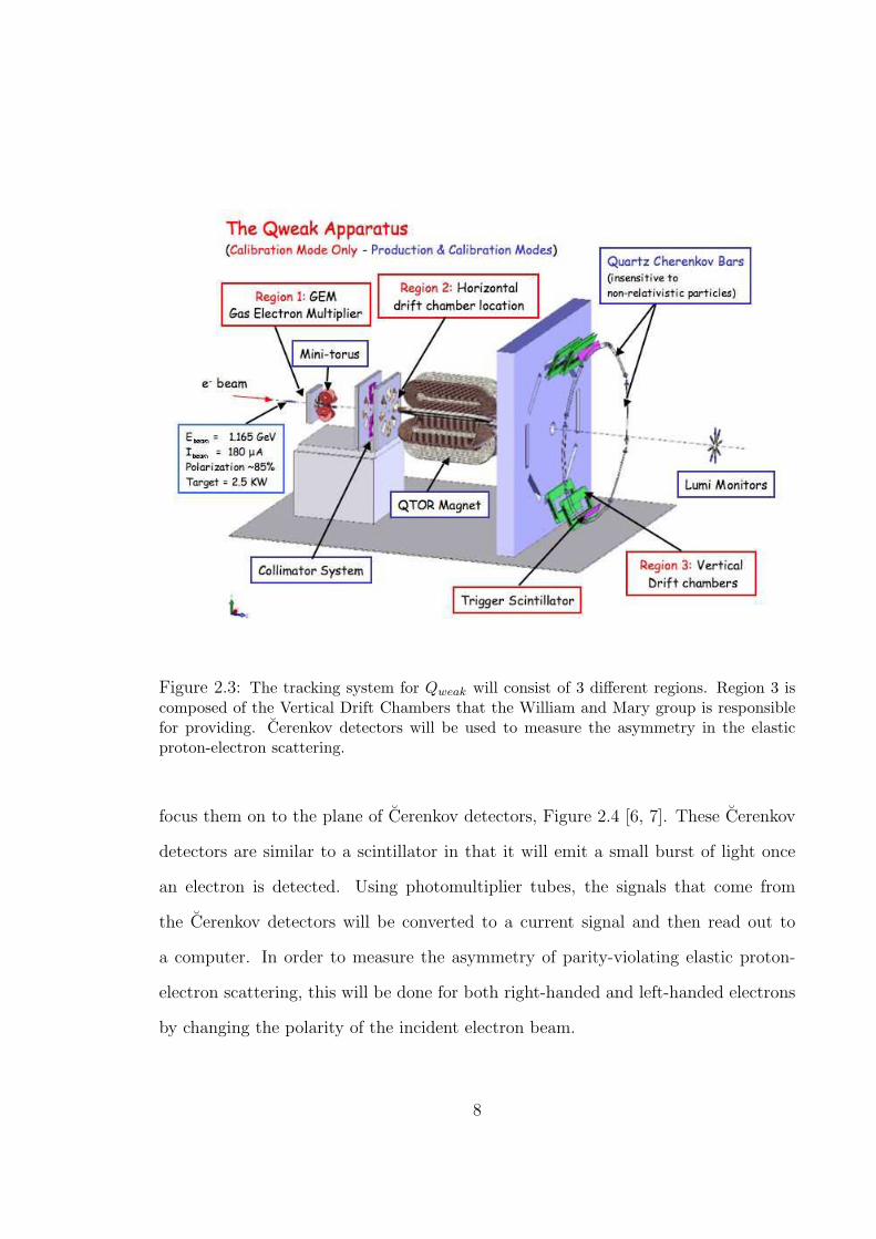
Figure 2.3: The tracking system for Qweak will consist of 3 different regions. Region 3 iscomposed of the Vertical Drift Chambers that the William and Mary group is responsiblefor providing. Cerenkov detectors will be used to measure the asymmetry in the elasticproton-electron scattering.
focus them on to the plane of Cerenkov detectors, Figure 2.4 [6, 7]. These Cerenkov
detectors are similar to a scintillator in that it will emit a small burst of light once
an electron is detected. Using photomultiplier tubes, the signals that come from
the Cerenkov detectors will be converted to a current signal and then read out to
a computer. In order to measure the asymmetry of parity-violating elastic proton-
electron scattering, this will be done for both right-handed and left-handed electrons
by changing the polarity of the incident electron beam.
8
Figure 2.4: This figure illustrates the path that the beamline takes as it passes throughthe experimental setup of Qweak. The beamline is incident on a liquid hydrogen target andthen passes through a precision collimator that selects out the electrons with a particularscattering angle. The toroidal magnet then bends the elastically scattered electrons awayfrom the beamline to the Cerenkov detectors.
9

2.4 Tracking System
A tracking system, consisting of three different regions, will be used periodically
to make subsidising measurements of the momentum transfer, Q2 [6]. For elastic
scattering, the momentum transfer is given by
Q2 =4E2sin2 θ
2
1 + 2 E
Msin2 θ
2
, (2.5)
where E is the incident electron energy, θ the scattering angle and M the proton
mass. Hence, knowing the incident electron energy and the scattering angle, the
measurement of the momentum transfer can be made. The incident electron energy
will be determined with ≤0.1% precision using the Hall C energy measurement system
[6]. The collimator that will be used will allow for a precision measurement of the
scattering angle of the elastically scattered electrons.
However, to ensure the electrons that were detected by the Cerenkov detectors
were indeed elastically scattered from the proton target, the tracking system will also
allow for the recreation of the electron’s path or track. The beam current will be
turned down from 180µA to approximately 10pA because the large beam current
would destroy the chambers used during the tracking. Region 1 will determine the
location of the elastically scattered electrons as they emerge from the collimator.
Region 2 will determine the position of the scattered electrons right before they enter
the toroidal magnet. Hence, the spatial distance between Region 1 and Region 2
will define the scattering angle that the elastically scattered electrons traverse before
entering the magnet [6]. Region 3 will consist of two Vertical Drift Chambers (VDC’s)
and will momentum-analyze events in order to ensure that the electrons that enter the
Cerenkov detectors were indeed elastically scattered. These chambers will determine
the trajectories, measuring position and angle, of events that take place, from which
10

Figure 2.5: Chambers are placed at opposing octants so that two measurements can bemade at a time. A total of 4 measurements will need to be made in order to cover the entiredetector system.
a measurement of the momentum can be made.
The William and Mary group has taken up the design and construction of the
Region 3 Vertical Drift Chambers. These chambers will be mounted to rotating wheel
(Ferris wheel design) that will allow for measurements in two opposing octants. See
Figure 2.5. Thus a total of four separate measurements will be needed in order to cover
the entire detector system. These types of measurements will be made approximately
every few weeks during a 2-year-long data-taking process.
2.4.1 Drift Chambers
Drift chambers are gas-filled devices that contain an array of wires and use
a high electric field to detect charged particles. For purposes of Qweak, the Region
3 vertical drift chambers will be used to determine the location and angle of the
11
primary electron after the magnetic field resulting from the elastic proton-electron
scattering. Wires are spaced approximately 5mm apart from one another and are
held at ground, while high voltage is applied to the chamber in order to generate a
large electric field within the chamber. The velocity of an electron as it traverses
through the chamber is determined by the type of gas mixture that is used. Previous
experiments that used vertical drift chambers have used an Argon/Ethane mixture
inside their chambers. This mixture has unique properties in that the drift velocity of
an electron is relatively constant. However, it has not been decided if this gas mixture
or another (such as Argon/CO2/Methane, which will be used in testing the vertical
drift chambers) will be used for Qweak. Although the electrons accelerate due to the
electric field, they collide with the gas molecules causing them to slow down. This
process of accelerating and colliding with gas molecules continues until the electron
reaches a wire within the chamber, and results in a constant drift velocity.
As an electron passes through the chamber and collides with the gas, it ionizes
the gas within the chamber (primary ionization), producing more electrons and ions
that are accelerated by the large electric field. As a result of the electric field, these
primary electrons drift towards the anode wires. However, the electric field, E, at the
wires is very large and so when the primary electron drifts near a wire, it undergoes
a large acceleration causing a build up of ionization around the wire; this is known
as the avalanche effect. The electrons trigger the sense wires upon which a signal is
sent out to the data collecting electronics that are attached to the chamber. The drift
time, the time that elapses for the first electron to trigger a wire, along with the drift
velocity is used to determine the distance travelled by the electron that triggered the
wire. Knowing several of these drift distances for several wires in the chamber can be
used to determine the track of the primary scattered electron.
12
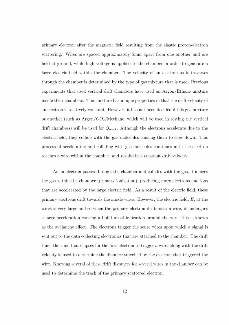
2.4.2 Vertical Drift Chambers
Vertical Drift Chambers (VDCs) are a type of drift chamber that tracks the
primary electron by triggering on ionization that has travelled in the vertical direction.
Figure 2.6 shows the operating principle of a Vertical Drift Chamber that will be used
for Qweak. As described, when the primary electron enters the chamber, it ionizes
the gas producing more electrons that drift in a vertical direction due to how the
electric field is applied to the chamber. Negative high voltage will be applied to
the chambers in order to generate the large electric fields needed to accelerate the
electrons. Therefore, ions that are created will drift to cathode planes while the
primary electrons will drift towards the anode-sense wires of the chamber, which are
held at ground. The drift time of these events is determined and since the drift
velocity of the particles is relatively constant (due to the acceleration and collisions
with the gas) the drift distances of the electrons can be computed. By knowing
this drift distance, since these electrons “drifted” in the vertical direction, one can
trace backwards to determine where the primary scattered electron was located in the
chamber. This process can be repeated for multiple primary electrons that resulted
from the scattered electron and a track of the scattered electron can be generated.
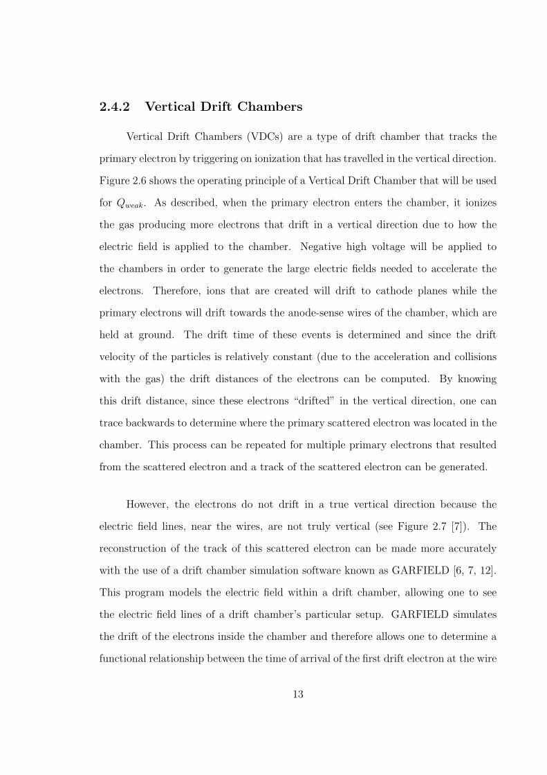
However, the electrons do not drift in a true vertical direction because the
electric field lines, near the wires, are not truly vertical (see Figure 2.7 [7]). The
reconstruction of the track of this scattered electron can be made more accurately
with the use of a drift chamber simulation software known as GARFIELD [6, 7, 12].
This program models the electric field within a drift chamber, allowing one to see
the electric field lines of a drift chamber’s particular setup. GARFIELD simulates
the drift of the electrons inside the chamber and therefore allows one to determine a
functional relationship between the time of arrival of the first drift electron at the wire
13
Figure 2.6: A cross section of a Vertical Drift Chamber that will be used in Qweak. Thetop and bottom lines are the high voltage planes that create the large electric fields withinthe chamber. The black dots through the center is a plane of the wires used to detect theionized electrons. The region highlighted in red is the region that could be triggered byionized electrons that result from the incoming track. L represents the the distance fromthe top of the plane to the wire plane, ℓ represents the length along the chamber from wherethe primary electron first enters the chamber and exits the chamber. β is the angle of theincoming electron.
and the perpendicular distance to the location of the primary electron. By knowing
this perpendicular distance, one can extrapolate from the sense wire to determine
the location at which the primary scattered electron. This process is repeated for
multiple wires in order to reconstruct a single track. With this reconstructed track
and the track information from Regions 1 and 2, and by studying the light output
of the Cerenkov detectors as a function of the location/angle of the incident track,
experimenters are able to determine if the scattered electron resulted from an elastic
or inelastic event.
14
Figure 2.7: This figure illustrates the electric field lines within a Vertical Drift Chamberas a result of a GARFIELD simulation. As one can see, the electric field lines near a wireare not vertical, and therefore the path of an electron near a wire is not going to be inthe vertical direction. Avalanche amplification is of the order 106 and occurs in the regionsnear the wires. With GARFIELD, one is able to better determine where the drift electronresulted from, causing the reconstructed track to be more accurate.
15
Chapter 3
Construction of Vertical Drift
Chamber
The William and Mary group has been working on the construction of these
vertical drift chambers, being extremely precise and careful in their steps to build the
chamber. Overall, the group will need to build a total of 5 of these drift chambers,
which 4 (2 in each octant) will be used at one time and the extra will serve as a
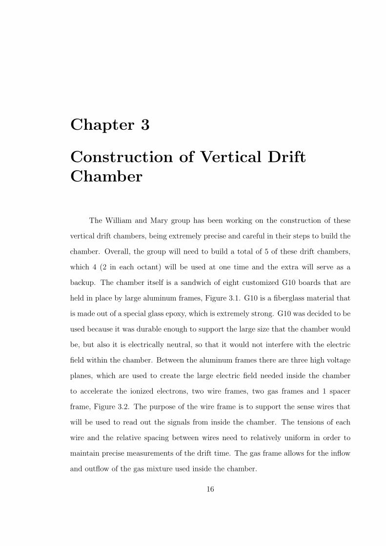
backup. The chamber itself is a sandwich of eight customized G10 boards that are
held in place by large aluminum frames, Figure 3.1. G10 is a fiberglass material that
is made out of a special glass epoxy, which is extremely strong. G10 was decided to be
used because it was durable enough to support the large size that the chamber would
be, but also it is electrically neutral, so that it would not interfere with the electric
field within the chamber. Between the aluminum frames there are three high voltage
planes, which are used to create the large electric field needed inside the chamber
to accelerate the ionized electrons, two wire frames, two gas frames and 1 spacer
frame, Figure 3.2. The purpose of the wire frame is to support the sense wires that
will be used to read out the signals from inside the chamber. The tensions of each
wire and the relative spacing between wires need to relatively uniform in order to
maintain precise measurements of the drift time. The gas frame allows for the inflow
and outflow of the gas mixture used inside the chamber.
16
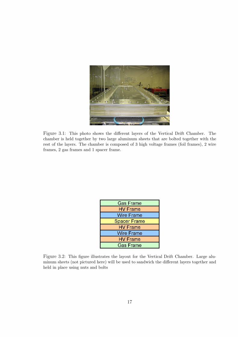
Figure 3.1: This photo shows the different layers of the Vertical Drift Chamber. Thechamber is held together by two large aluminum sheets that are bolted together with therest of the layers. The chamber is composed of 3 high voltage frames (foil frames), 2 wireframes, 2 gas frames and 1 spacer frame.
Figure 3.2: This figure illustrates the layout for the Vertical Drift Chamber. Large alu-minum sheets (not pictured here) will be used to sandwich the different layers together andheld in place using nuts and bolts
17

Figure 3.3: This photo illustrates the 4 different components that the G10 frames wereconstructed out of. These four components were epoxied and clamped together to createthe G10 frame.
The G10 frames were constructed from four separate pieces which were epoxied
together, Figure 3.3 and 3.4. In order to ensure this connection would hold, each
corner of the frames were clamped down until the epoxy set. The G10 frames also
needed to be cleaned very well using acetone in order to ensure that dirt or dust
particles would interfere with measurements inside the chamber. For the high voltage
and gas frames (Figure 3.5), a conductive aluminized mylar foil was stretched across
the G10 using a specifically designed lab table (Figure 3.6) and then epoxied in place.
The purpose of the mylar is to hold the high voltage potential to create the large
electric field needed inside the chamber. In order to ensure an electrical connection
between the mylar and high voltage potential that would generate the electric field,
a strip of tin-coated copper strips were placed inside a machined groove around the
perimeter of the frame and held in place using a conductive epoxy, Figure 3.7. The
wire frames (Figure 3.8) were carefully made using 25µm gold-plated tungston wire,
with each frame containing 280 wires. Each frame was then again cleaned and stored
away so that dust and other dirt particles would not penetrate the chamber.
18

Figure 3.4: This photo illustrates a typical completed G10 frame after the G10 componentshad been epoxied and clamped.
Figure 3.5: This photo shows the spacer frame positioned on top of a completed highvoltage (HV) frame that will be used in the Vertical Drift Chamber. High voltage will beapplied to the mylar in order to create a large electric field within the chamber that will beused to create ionization.
19
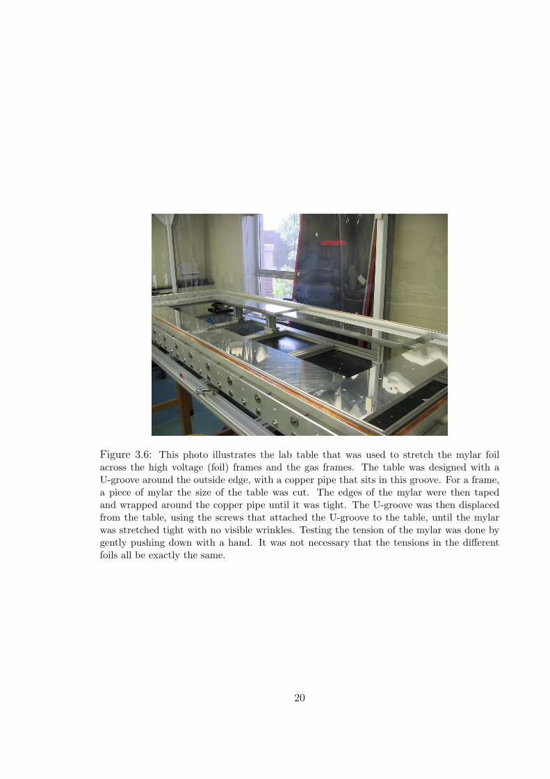
Figure 3.6: This photo illustrates the lab table that was used to stretch the mylar foilacross the high voltage (foil) frames and the gas frames. The table was designed with aU-groove around the outside edge, with a copper pipe that sits in this groove. For a frame,a piece of mylar the size of the table was cut. The edges of the mylar were then tapedand wrapped around the copper pipe until it was tight. The U-groove was then displacedfrom the table, using the screws that attached the U-groove to the table, until the mylarwas stretched tight with no visible wrinkles. Testing the tension of the mylar was done bygently pushing down with a hand. It was not necessary that the tensions in the differentfoils all be exactly the same.
20
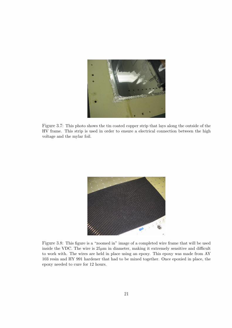
Figure 3.7: This photo shows the tin coated copper strip that lays along the outside of theHV frame. This strip is used in order to ensure a electrical connection between the highvoltage and the mylar foil.
Figure 3.8: This figure is a “zoomed in” image of a completed wire frame that will be usedinside the VDC. The wire is 25µm in diameter, making it extremely sensitive and difficultto work with. The wires are held in place using an epoxy. This epoxy was made from AY103 resin and HY 991 hardener that had to be mixed together. Once epoxied in place, theepoxy needed to cure for 12 hours.
21
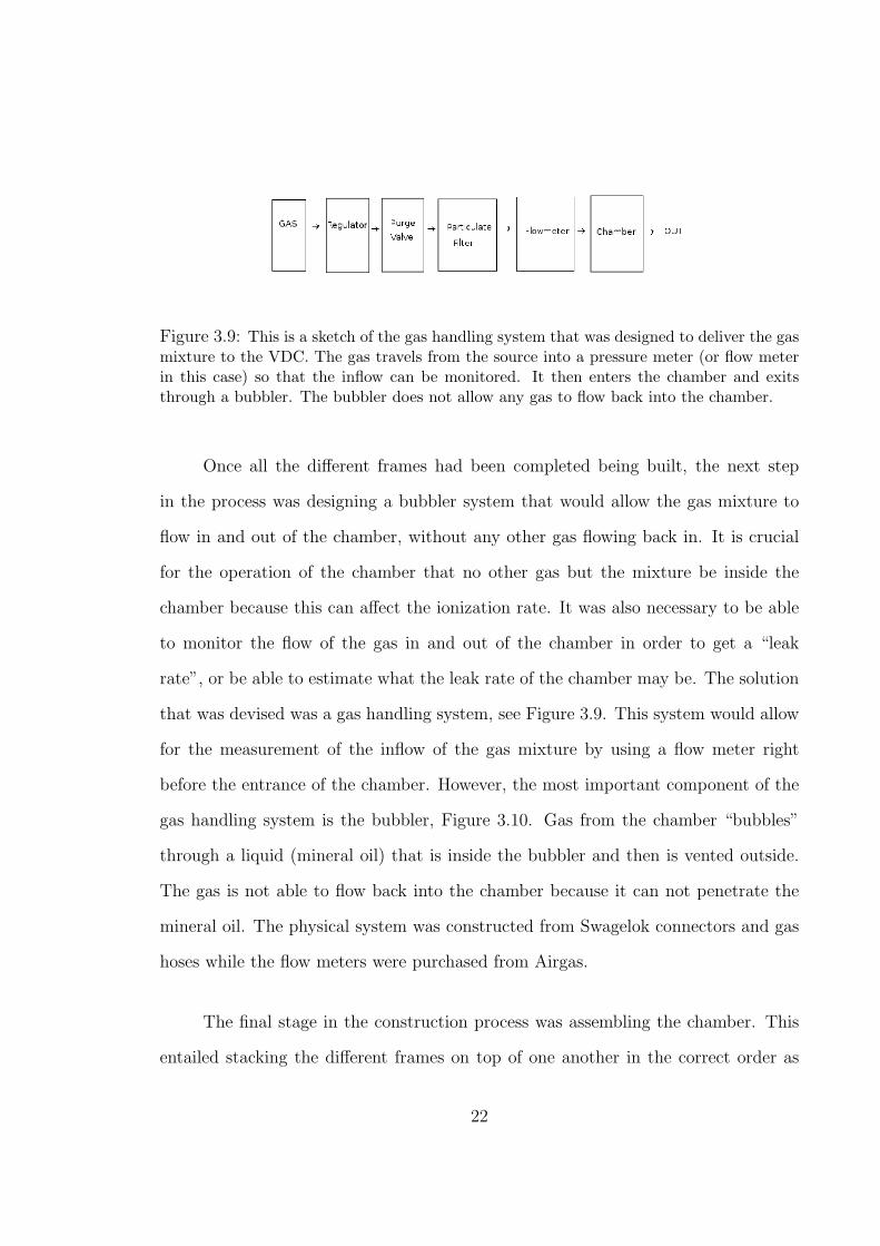
Figure 3.9: This is a sketch of the gas handling system that was designed to deliver the gasmixture to the VDC. The gas travels from the source into a pressure meter (or flow meterin this case) so that the inflow can be monitored. It then enters the chamber and exitsthrough a bubbler. The bubbler does not allow any gas to flow back into the chamber.
Once all the different frames had been completed being built, the next step
in the process was designing a bubbler system that would allow the gas mixture to
flow in and out of the chamber, without any other gas flowing back in. It is crucial
for the operation of the chamber that no other gas but the mixture be inside the
chamber because this can affect the ionization rate. It was also necessary to be able
to monitor the flow of the gas in and out of the chamber in order to get a “leak
rate”, or be able to estimate what the leak rate of the chamber may be. The solution
that was devised was a gas handling system, see Figure 3.9. This system would allow
for the measurement of the inflow of the gas mixture by using a flow meter right
before the entrance of the chamber. However, the most important component of the
gas handling system is the bubbler, Figure 3.10. Gas from the chamber “bubbles”
through a liquid (mineral oil) that is inside the bubbler and then is vented outside.
The gas is not able to flow back into the chamber because it can not penetrate the
mineral oil. The physical system was constructed from Swagelok connectors and gas
hoses while the flow meters were purchased from Airgas.
The final stage in the construction process was assembling the chamber. This
entailed stacking the different frames on top of one another in the correct order as
22
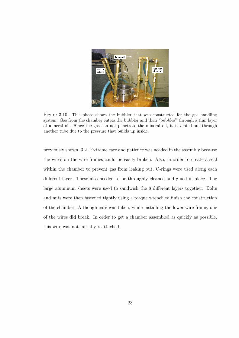
Figure 3.10: This photo shows the bubbler that was constructed for the gas handlingsystem. Gas from the chamber enters the bubbler and then “bubbles” through a thin layerof mineral oil. Since the gas can not penetrate the mineral oil, it is vented out throughanother tube due to the pressure that builds up inside.
previously shown, 3.2. Extreme care and patience was needed in the assembly because
the wires on the wire frames could be easily broken. Also, in order to create a seal
within the chamber to prevent gas from leaking out, O-rings were used along each
different layer. These also needed to be throughly cleaned and glued in place. The
large aluminum sheets were used to sandwich the 8 different layers together. Bolts
and nuts were then fastened tightly using a torque wrench to finish the construction
of the chamber. Although care was taken, while installing the lower wire frame, one
of the wires did break. In order to get a chamber assembled as quickly as possible,
this wire was not initially reattached.
23
Chapter 4
Testing of the Vertical Drift
Chamber
4.0.3 Overview
In order to see if the constructed chamber would operate properly, tests on the
chamber were next performed. Testing of the vertical drift chambers was done in
multiple steps, each step testing different components of the chamber. By testing
parts of the chamber, malfunctioning components could be pinpointed and repaired,
while operating parts could be verified that they were indeed functioning properly.
Testing was done in a three stage process as follows: First, the gas handling system
was tested to make sure that the gas would be effectively delivered to the chamber.
Next, high voltage was applied to the chamber in order to see if the chamber could
handle the voltage. Finally, using cosmic rays and a 90Sr beta source, detection of
tracks as well as the efficiencies of individual wires inside the chamber were tested.
4.0.4 Gas Handling System Testing
Overview
Testing of the gas handling system was important because it is vital that the
correct, pure gas mixture be inside the chamber during operation. Therefore, it
needed to verified that the bubbler was working properly and that no other gas
24
was getting inside the chamber. For example, O2 can “poison” the operation of the
chamber. Also, it was necessary to estimate a leak rate for the chamber to have
an idea about how much gas was escaping from the chamber. The leak rate will be
important for the main experiment because the gas mixture that will be used contains
ethane, and due to safety regulations at Jefferson Lab, a value (or estimate) of how
much gas escapes from the chamber should be known.
Testing Setup
To test the gas handling system as well as measure the leak rate of the chamber,
the chamber was connected to the gas handling system via the Swagelok connections
(Figure 4.1) which in return was connected to the Argon/Carbon Dioxide/Methane
(88%/10%/2%) mixture that would be used for testing. A regulator was connected to
the bottle containing the gas mixture so that the pressure of the bottle and the outflow
pressure could be monitored. Connected to the regulator was an (Y40-LF1728) Airgas
particle filter that filters out 100% of particles larger than 0.003µm that may be inside
the bottle of gas. An Airgas flowmeter was connected in series between the chamber
and the gas regulator and was used to monitor the gas flow into the chamber. Once the
system was connected, the gas was then turned on, upon which it filled the chamber.
It was observed that the gas from inside the chamber would bubble out through the
bubbler, however the bubbling rate was not at all constant. The cause for this, we
hypothesize, is due to a threshold pressure that the chamber must overcome to bubble
through the mineral oil that is inside the bubbler.
Results from Testing Bubbler
The leak rate for the chamber was determined to be approximately 0 ℓ
hr. This
was computed by observing the rate at which the bubbler would bubble as gas flowed
through the chamber. While gas is flowing through the chamber, it was noticed that
25

the aluminumized mylar that keeps the gas inside the chamber would expand and
contract. This was associated with a “breathing” effect that existed as a result of
the threshold pressure for the bubbler. Once the pressure inside the chamber met
this threshold, the chamber would “exhale” or expel the gas mixture through the
bubbler. Below this threshold, the bubbler would not bubble. It was observed that
with a flow rate of 21 ℓ
hr, the bubbler would bubble for 7 minutes and be off for 9
minutes. Repeating this with a flow rate of 29 ℓ
hrit was observed that the bubbler
would bubble for 14 minutes and then be off for 6 minutes. The difference in volume
due to the expansion and contraction of the aluminum mylar was determined to be
approximately 3 liters (out of a total volume of 111ℓ) by calculating the amount of
gas that flowed into the chamber during the time that the bubbler was not bubbling.
Once the bubbler stopped bubbling, the flow rate was then set to 2 ℓ
hrand it was
observed that the bubbler again bubbled in approximately 1.5 hours. Therefore, 3
liters of gas was delivered to the chamber (2 ℓ
hr* 1.5 hours) and since the difference
in volume due to the expansion and contraction of the mylar was 3 liters, very little
gas leaked from the chamber. A precise measurement of the leak rate of the chamber
was not necessary and so we concluded that the leak rate was approximately 0 ℓ
hr.
Similarily designed vertical drift chambers, used by Hall A at Jefferson Lab, had a
leak rate of 3 ℓ
hrfor 48ℓ chambers.
4.0.5 High Voltage Testing and Conditioning
Overview
The next part to testing the VDC was applying the high voltage that would
be used to generate the electric fields inside the chamber. The expected outcome of
these tests was to identify the voltage range that the drift chamber would require in
order to operate properly. This voltage would be determined by making a plot of the
26
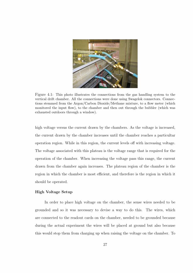
Figure 4.1: This photo illustrates the connections from the gas handling system to thevertical drift chamber. All the connections were done using Swagelok connectors. Connec-tions stemmed from the Argon/Carbon Dioxide/Methane mixture, to a flow meter (whichmonitored the input flow), to the chamber and then out through the bubbler (which wasexhausted outdoors through a window).
high voltage versus the current drawn by the chambers. As the voltage is increased,
the current drawn by the chamber increases until the chamber reaches a particultar
operation region. While in this region, the current levels off with increasing voltage.
The voltage associated with this plateau is the voltage range that is required for the
operation of the chamber. When increasing the voltage pass this range, the current
drawn from the chamber again increases. The plateau region of the chamber is the
region in which the chamber is most efficient, and therefore is the region in which it
should be operated.
High Voltage Setup
In order to place high voltage on the chamber, the sense wires needed to be
grounded and so it was necessary to devise a way to do this. The wires, which
are connected to the readout cards on the chamber, needed to be grounded because
during the actual experiment the wires will be placed at ground but also because
this would stop them from charging up when raising the voltage on the chamber. To
27

Figure 4.2: This figure illustrates how the readout cards and therefore the sense wires weregrounded while applying high voltage to the drift chamber. Small aluminum rods weresoldered to each DIN pin connector and then wires were soldered to each of the aluminumrods. The aluminum rods were connected to one another using a grounding wire. Theend of the grounding wire was then taped on to the aluminum frame to ensure a groundconnection.
ground the wires, 1
8” aluminum rods were soldered on to the DIN pin connectors that
attach to the readout cards. Wires were then soldered to each of the aluminum rods,
which were then connected to a grounding wire. This grounding wire connected all
the readout cards to one another, Figure 4.2. The end of the grounding wire was
then connected to the aluminum frame of the chamber via a piece of electrical tape,
creating a common ground.
A transition box that would take the safe high voltage (SHV) connection from
the high voltage (HV) power supply to the chamber also needed to be made. The high
voltage is generated from a single channel of a Bertan negative high voltage (model
377N) power supply. The output from the power supply was ran through an RC pro-
tection circuit that used a 1MΩ resistor and 330pF capacitor. This protection circuit
prevents any large spikes in current that could occur when increasing the voltage on
the chamber to large values. This output was then connected to 3 silicone-coated
28
high voltage wires, (called SIL-KOAT, 500 feet spool) each of which are connected to
the cathode planes of the drift chamber. The diameter of the wire is 2mm and was
chosen because it is rated to a maximum of 20kV with no corona discharge.
Results from Testing and Conditioning
Once the sense wires were grounded and the transition box in place, the voltage
was turned on. First, only 100 V was placed on the chamber so that a multimeter
could be used to check that the sense wires and outer aluminum frames of the chamber
were properly grounded. The voltage was then slowly increased. To ensure the safety
of the chamber, the trip setpoint was set to 100µA scale. This trip setpoint acts
similar to an adjustable breaker box in that the voltage is “tripped” when the current
exceeds 80% of the setpoint limit. (In this case, the trip setpoint was set at the 100µA
scale, the circuit would trip if the current being drawn reached 80µA.) The first trip
occurred at a voltage of 1.1kV. These trips are associated with “training” the drift
chamber. In training a chamber, dust particles and other dirt is burned off as the
voltage is ramped up and the chamber “learns” how to handle higher voltages. During
the beginning stages of training the chamber, the voltage and quiescent currents were
recorded, Tables 4.1 and 4.2.
It was observed that the current increased as the voltage on the chamber in-
creased. However, the difference between these two tables is that the data from Table
4.2 was observed after a longer period of time had elapsed with the voltage on the
chamber. During this time, the voltage did not trip off and remained steady. It
was observed that for the lower voltages (2.0kV - 2.7kV), the currents drawn by the
chamber had decreased with respect to the currents in Table 4.1. This decrease cor-
responds to the conditioning of the drift chamber. This data supports the idea that
as time elapsed with voltage applied to the chamber, more dust and other debris that
29

could cause corona discharge, sparking or arcing (and therefore current to be drawn)
inside the chamber were burned off causing the decrease in current. Since the current
levels were decreased by this conditioning, larger voltages were able to be applied to
the chamber. Again, this process of leaving the voltage on the chamber for a period
of time and allowing for conditioning was repeated for these larger voltages.
Voltage (kV) Current (µA)1.9 0.02 ± 0.0012.0 0.04 ± 0.0012.1 0.09 ± 0.0022.2 0.16 ± 0.0052.3 0.23 ± 0.0082.4 0.32 ± 0.012.5 0.42 ± 0.0152.6 0.50 ± 0.022.7 0.78 ± 0.023
Table 4.1: During the training of the drift chamber, voltages and the associated current atthat voltage were recorded. As the voltage is increased, the current on the drift chamberincreases, however, there should be a point at which the current begins to level off withincreasing voltage. This is known as the plateau and is also the operating region of the driftchamber. After the plateau region, the current again increases with increases in voltage.
Although conditioning had been observed, when raising the voltage on the cham-
ber to a value of 3.35kV the current drawn by the chamber was initially 14µA. The
chamber was left at this voltage for a period of 24 hours in the hope of lowering the
current. However, after the 24 hours, the current increased to 17µA, and therefore
the chamber did not seem to be conditioning any further. However, as one can see
from Figure 4.3 and Figure 4.4, the plateau region had not been reached and so the
chamber needed to be able to support larger voltages. In order to determine where on
the chamber the current was being drawn, an ammeter was used to read the current
passing through each of the readout cards. It was found that 95% of the current being
30

1 1.5 2 2.5 3 3.5 4Voltage (V)
0
5
10
15
20
Cur
rent
(µA
)
Initial Conditioning of Vertical Drift Chamber
Figure 4.3: This plot shows the initial conditioning of the drift chamber. The blue pointsare values that were first obtained before allowing time to elapse with voltage on the cham-ber. The red points are values that were later obtained after allowing the voltage to beapplied to the chamber for a period of time. Values were unable to be collected for largervoltages initially because the currents being drawn were much too high. However, there isevidence of some coniditioning since the currents seem to have decreased after allowing volt-age to be applied to the chamber. The error bars on the plot were determined by watchingthe current oscillate using an ammeter while a particular voltage was applied.
31
1 1.5 2 2.5 3 3.5 4Voltage (V)
1e-05
0.0001
0.001
0.01
0.1
1
10
Cur
rent
(µA
)
Initial Conditioning of Vertical Drift Chamber
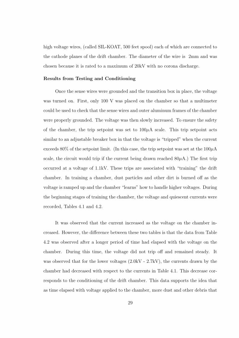
Figure 4.4: This log plot shows the initial conditioning of the drift chamber. The bluepoints are values that were first obtained before allowing time to elapse with voltage onthe chamber. The red points are values that were later obtained after allowing the voltageto be applied to the chamber for a period of time. There is evidence of a plateau in thecurrent (operating region) around 3.4kV.
32

Voltage (kV) Current (µA)2.0 0.00 ± 02.1 0.03 ± 0.0012.2 0.07 ± 0.0032.3 0.12 ± 0.0042.4 0.20 ± 0.0072.5 0.31 ± 0.0112.6 0.45 ± 0.0132.7 0.65 ± 0.0172.8 0.90 ± 0.0212.9 1.23 ± 0.0293.0 1.65 ± 0.0313.1 2.19 ± 0.0543.2 4.14 ± 0.0713.3 17.4 ± 2.23
Table 4.2: The voltage was left on the chamber for approximately 8 hours before thisdata was collected. The voltage did not trip off during this period of conditioning. Itwas observed that the currents associated with lower voltages decreased with respect to thevalues of current from Table 4.1. This supports the notion that the chamber was undergoinga conditioning process. Since the current decreased, higher voltages were able to be appliedto the chamber. These voltages corresponded with large currents being drawn.
drawn was coming from the adjacent wires on the right and left of the single wire
that had broken during assembly. In order to fix this, the chamber was disassembled
and the missing wire was replaced. With the chamber apart, spots were observed on
the aluminum mylar, Figure 4.5, which is evidence that arcing within the chamber
had occured when applying high voltage.
The chamber was reassembled and testing high voltage on the chamber resumed.
With the wire replaced, the current that the chamber was drawing when a voltage of
3.35 kV was applied was now at 0.52µA. This was a significant change in current that
was observed with the wire missing (17µA). In order to “see” what was happening
inside the chamber with a missing wire, a GARFIELD simulation was ran with and
33
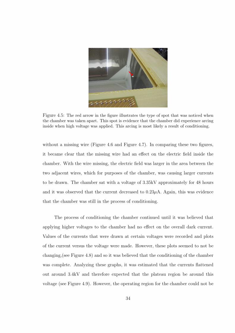
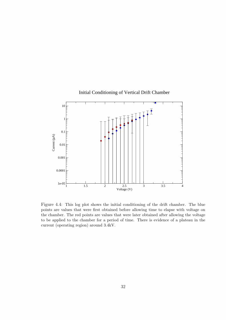
Figure 4.5: The red arrow in the figure illustrates the type of spot that was noticed whenthe chamber was taken apart. This spot is evidence that the chamber did experience arcinginside when high voltage was applied. This arcing is most likely a result of conditioning.
without a missing wire (Figure 4.6 and Figure 4.7). In comparing these two figures,
it became clear that the missing wire had an effect on the electric field inside the
chamber. With the wire missing, the electric field was larger in the area between the
two adjacent wires, which for purposes of the chamber, was causing larger currents
to be drawn. The chamber sat with a voltage of 3.35kV approximately for 48 hours
and it was observed that the current decreased to 0.23µA. Again, this was evidence
that the chamber was still in the process of conditioning.
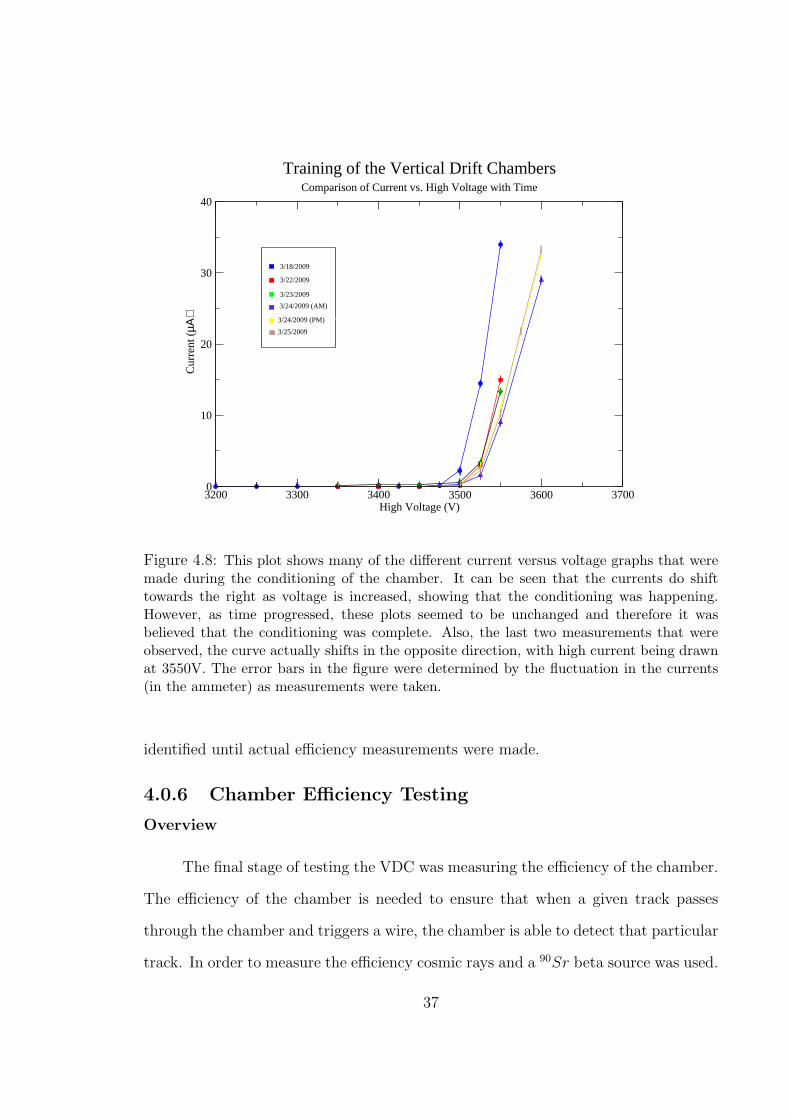
The process of conditioning the chamber continued until it was believed that
applying higher voltages to the chamber had no effect on the overall dark current.
Values of the currents that were drawn at certain voltages were recorded and plots
of the current versus the voltage were made. However, these plots seemed to not be
changing,(see Figure 4.8) and so it was believed that the conditioning of the chamber
was complete. Analyzing these graphs, it was estimated that the currents flattened
out around 3.4kV and therefore expected that the plateau region be around this
voltage (see Figure 4.9). However, the operating region for the chamber could not be
34
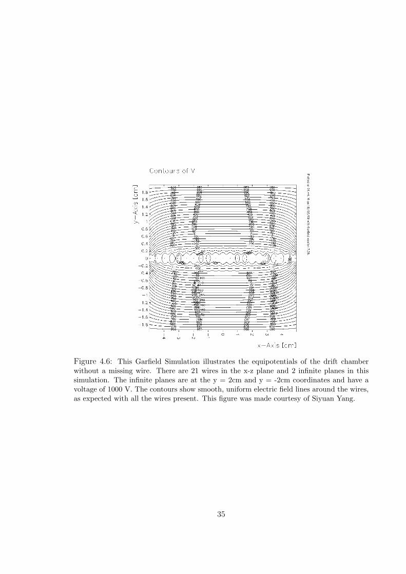
Figure 4.6: This Garfield Simulation illustrates the equipotentials of the drift chamberwithout a missing wire. There are 21 wires in the x-z plane and 2 infinite planes in thissimulation. The infinite planes are at the y = 2cm and y = -2cm coordinates and have avoltage of 1000 V. The contours show smooth, uniform electric field lines around the wires,as expected with all the wires present. This figure was made courtesy of Siyuan Yang.
35
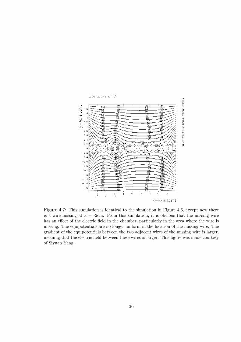
Figure 4.7: This simulation is identical to the simulation in Figure 4.6, except now thereis a wire missing at x = -2cm. From this simulation, it is obvious that the missing wirehas an effect of the electric field in the chamber, particularly in the area where the wire ismissing. The equipotentials are no longer uniform in the location of the missing wire. Thegradient of the equipotentials between the two adjacent wires of the missing wire is larger,meaning that the electric field between these wires is larger. This figure was made courtesyof Siyuan Yang.
36
3200 3300 3400 3500 3600 3700High Voltage (V)
0
10
20
30
40C
urre
nt (
µΑ)
Training of the Vertical Drift ChambersComparison of Current vs. High Voltage with Time
3/18/2009
3/22/2009
3/23/2009
3/24/2009 (AM)
3/24/2009 (PM)3/24/2009 (PM)
3/25/2009
Figure 4.8: This plot shows many of the different current versus voltage graphs that weremade during the conditioning of the chamber. It can be seen that the currents do shifttowards the right as voltage is increased, showing that the conditioning was happening.However, as time progressed, these plots seemed to be unchanged and therefore it wasbelieved that the conditioning was complete. Also, the last two measurements that wereobserved, the curve actually shifts in the opposite direction, with high current being drawnat 3550V. The error bars in the figure were determined by the fluctuation in the currents(in the ammeter) as measurements were taken.
identified until actual efficiency measurements were made.
4.0.6 Chamber Efficiency Testing
Overview
The final stage of testing the VDC was measuring the efficiency of the chamber.
The efficiency of the chamber is needed to ensure that when a given track passes
through the chamber and triggers a wire, the chamber is able to detect that particular
track. In order to measure the efficiency cosmic rays and a 90Sr beta source was used.
37
3200 3300 3400 3500 3600 3700High Voltage (V)
1e-06
1e-05
0.0001
0.001
0.01
0.1
1
10
Cur
rent
(µΑ
)
Training of the Vertical Drift ChambersComparison of Current vs. High Voltage with Time
3/18/2009
3/22/2009
3/23/2009
3/24/2009 (AM)
3/24/2009 (PM)3/24/2009 (PM)
3/25/2009
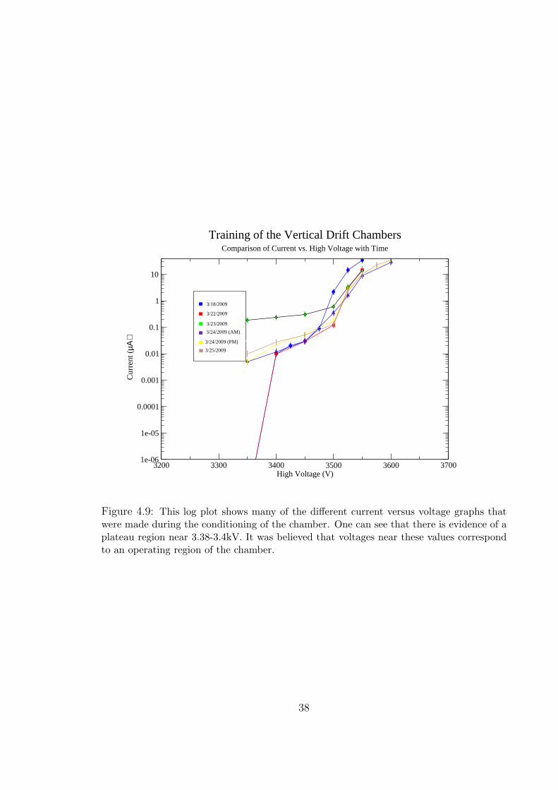
Figure 4.9: This log plot shows many of the different current versus voltage graphs thatwere made during the conditioning of the chamber. One can see that there is evidence of aplateau region near 3.38-3.4kV. It was believed that voltages near these values correspondto an operating region of the chamber.
38

Figure 4.10: This image shows the NIM modules that were used for measuring the efficiencyof the drift chamber.
It was expected that as the voltage on the chamber was increased, the efficiency would
improve. Also, after having defined a plateau region for the chamber, it was expected
that the efficiency of the chamber would be the greatest within this region. To
measure the efficiency Nuclear Instrumentation Modules (NIM) were used to analyze
the signals detected by the chamber, Figure 4.10.
Initial Testing and Results
A single readout card was selected from the bottom wire plane. The first three
wires from this card were selected using alligator clip to BNC cables, with the grounds
of the cable being connected to the ground of the frame. The rest of the sense wires
from the readout card were grounded. The BNC cable from the 3 wires were then sent
to separate channels of a Phillips amplifier module (Model 776) in which the signals
were amplified twice, with each stage amplifying by ×10, for a total amplification of
100. This amplification was done so that the electronics would be able to detect small
signals. The amplified signal was then sent to NIM (Model 711) discriminators and
then to a NIM (Model 754) coincidence module. The purpose of the discriminator
39
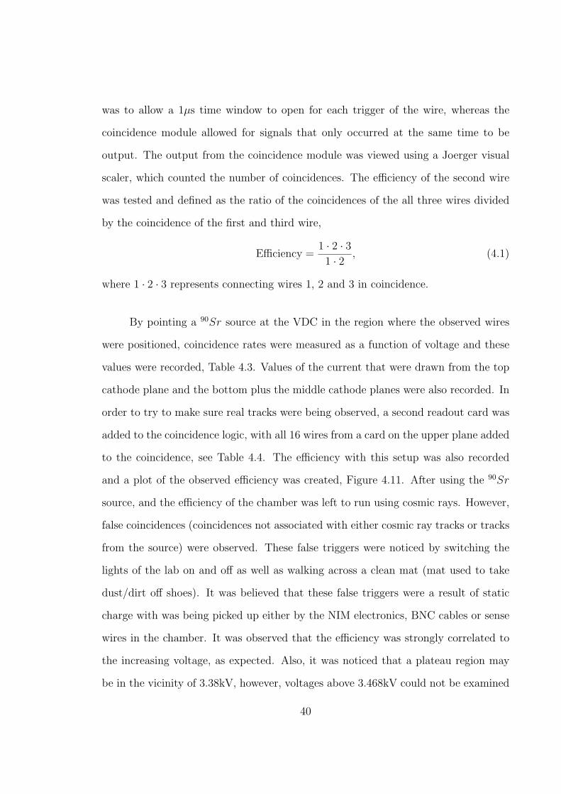
was to allow a 1µs time window to open for each trigger of the wire, whereas the
coincidence module allowed for signals that only occurred at the same time to be
output. The output from the coincidence module was viewed using a Joerger visual
scaler, which counted the number of coincidences. The efficiency of the second wire
was tested and defined as the ratio of the coincidences of the all three wires divided
by the coincidence of the first and third wire,
Efficiency =1 · 2 · 31 · 2
, (4.1)
where 1 · 2 · 3 represents connecting wires 1, 2 and 3 in coincidence.
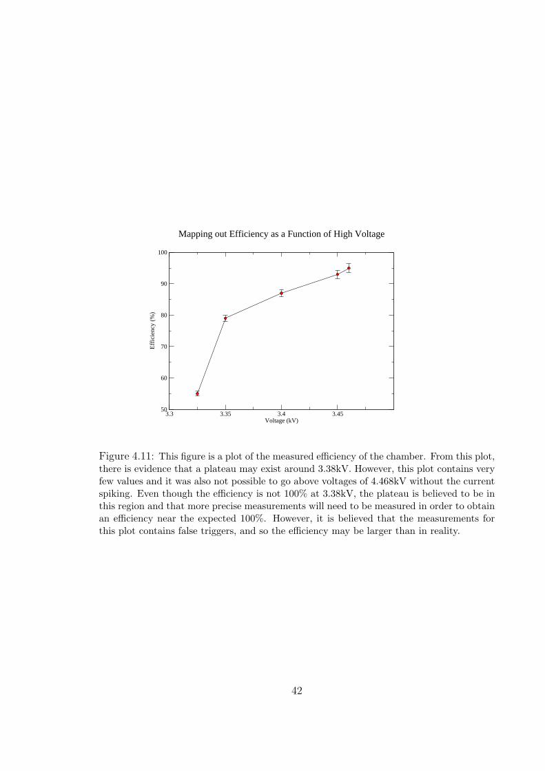
By pointing a 90Sr source at the VDC in the region where the observed wires
were positioned, coincidence rates were measured as a function of voltage and these
values were recorded, Table 4.3. Values of the current that were drawn from the top
cathode plane and the bottom plus the middle cathode planes were also recorded. In
order to try to make sure real tracks were being observed, a second readout card was
added to the coincidence logic, with all 16 wires from a card on the upper plane added
to the coincidence, see Table 4.4. The efficiency with this setup was also recorded
and a plot of the observed efficiency was created, Figure 4.11. After using the 90Sr
source, and the efficiency of the chamber was left to run using cosmic rays. However,
false coincidences (coincidences not associated with either cosmic ray tracks or tracks
from the source) were observed. These false triggers were noticed by switching the
lights of the lab on and off as well as walking across a clean mat (mat used to take
dust/dirt off shoes). It was believed that these false triggers were a result of static
charge with was being picked up either by the NIM electronics, BNC cables or sense
wires in the chamber. It was observed that the efficiency was strongly correlated to
the increasing voltage, as expected. Also, it was noticed that a plateau region may
be in the vicinity of 3.38kV, however, voltages above 3.468kV could not be examined
40

because the current being drawn from the chambers began to spike.
HV (kV) Threshold (mV) T Current (µA) M+B Current (µA) Efficiency
3.30 700 0.10 ± 0.01 0.27 ± 0.03 No Efficiency3.35 700 0.13 ± 0.03 0.33 ± 0.04 75 ± 0.043.38 700 0.18 ± 0.04 0.41 ± 0.05 92 ± 0.013.40 700 0.22 ± 0.04 0.5 ± 0.05 90 ± 0.023.40 900 0.23 ± 0.04 0.55 ± 0.05 94 ± 0.0083.45 500 0.55 ± 0.06 1.0 ± 0.08 88 ± 0.0083.45 700 0.70 ± 0.08 1.2 ± 0.08 95 ± 0.0073.45 900 0.58 ± 0.06 1.1 ± 0.08 98 ± 0.0063.468 700 5.2 ± 0.23 5.4 ± 0.24 96 ± 0.006
Table 4.3: This table shows the data that was collected while testing the efficiency ofthe chamber with the 90Sr source. “T Current” represents the current that was drawnfrom the upper foil frame. “M+B” represents the current that was drawn from the middleand bottom foil frames. The threshold in this data represents the threshold at which theNIM discriminator was set. This threshold sets the limit at which the discriminator willfire. One can see that there is a relationship between the voltage on the chamber and theefficiency, as expected. It was also observed that there was a relationship between adjustingthe threshold of allowed signals and the efficiency.
HV(V) Threshold (mV) T Current (µA) M+B Current (µA) Efficiency
3.30 500 0.10 ± 0.01 0.26 ± 0.04 No Efficiency3.325 500 0.12 ± 0.03 0.31 ± 0.06 55 ± 0.113.35 500 0.14 ± 0.03 0.35 ± 0.06 79 ± 0.043.40 500 0.23 ± 0.04 0.55 ± 0.07 87 ± 0.023.45 500 0.56 ± 0.07 1.1 ± 0.09 93 ± 0.013.460 500 2.6 ± 0.11 3.0 ± 0.12 95 ± 0.007
Table 4.4: This table shows the data that was collected while testing the efficiency of thechamber with the 90Sr source while including the coincidence of the top readout card. ‘TCurrent” represents the current that was drawn from the upper foil frame. “M+B” repre-sents the current that was drawn from the middle and bottom foil frames. The threshold inthis data represents the threshold at which the NIM discriminator was set. This thresholdsets the limit at which the discriminator will fire. One can see that there is a relationshipbetween the voltage on the chamber and the efficiency, as expected. It was also observedthat there was a relationship between adjusting the threshold of allowed signals and theefficiency.
41
3.3 3.35 3.4 3.45Voltage (kV)
50
60
70
80
90
100
Eff
icie
ncy
(%)
Mapping out Efficiency as a Function of High Voltage
Figure 4.11: This figure is a plot of the measured efficiency of the chamber. From this plot,there is evidence that a plateau may exist around 3.38kV. However, this plot contains veryfew values and it was also not possible to go above voltages of 4.468kV without the currentspiking. Even though the efficiency is not 100% at 3.38kV, the plateau is believed to be inthis region and that more precise measurements will need to be measured in order to obtainan efficiency near the expected 100%. However, it is believed that the measurements forthis plot contains false triggers, and so the efficiency may be larger than in reality.
42
Further Chamber Efficiency Testing, Problems and Results
Ideally, the chambers should only detect true cosmic ray tracks, i.e. tracks that
travel in a straight line, and propogate through the chamber. However, during the
initial phase of testing the efficiency of the chambers, there was concern that the
chambers were detecting background noise and cosmic ray events that may not be
associated with a single straight track. In order to account for these different events,
coincidences were added to the electronics. Scintillators were placed on top of and
below the drift chamber, with both signals placed in coincidence with each other.
This coincidence was then added to the previous circuit. An antenna was also added
as a veto to the coincidences in order to account for the background noise in the
lab. The antenna consisted of a BNC to alligator clips cable, with one alligator clip
hanging in mid air and the other alligator clip grounded to the frame of the chamber.
Figure 4.12 is a logic diagram of the electronics and Figure 4.13 is a timing diagram of
the circuit. With the new coincidences added, the measured efficiency was calculated
using equation
Efficiency =1 · 2 · 3 · SCINT
1 · 2 · SCINT. (4.2)
Measurements of the chamber efficiency were again measured at different volt-
ages, but it still remained unclear if the background noise was eliminated with the
addition of more inputs into the coincidence logic. It was decided that instead of
using BNC to alligator clip cables and NIM amplifier/discriminator for the electron-
ics that the switch to the MAD preamp/discriminator chip [6] be made, Figure 4.14.
This particular chip attaches directly to the readout card on the chamber and will be
used in the experiment at Jefferson Lab. The advantage of using this card, is that
the signals should be less noise-sensitive since the electronics is located right at the
readout card and also different wires on a readout card could be monitored at a time.
43
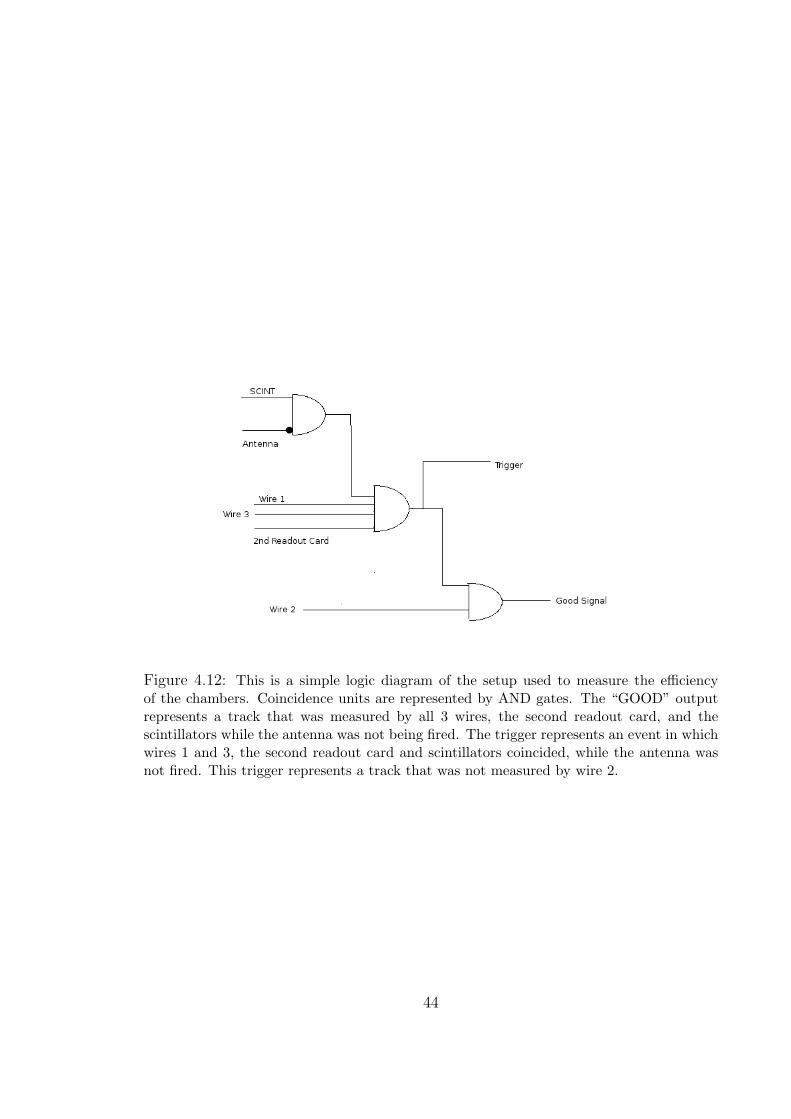
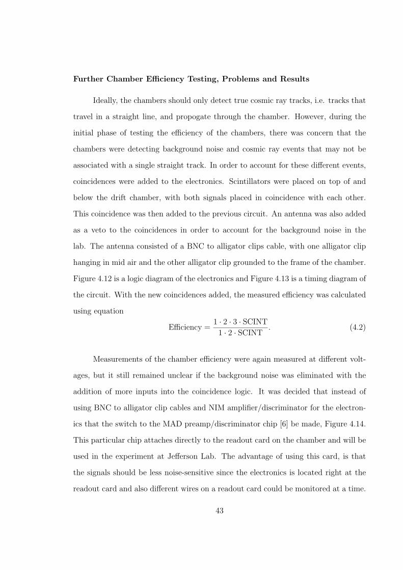
Figure 4.12: This is a simple logic diagram of the setup used to measure the efficiencyof the chambers. Coincidence units are represented by AND gates. The “GOOD” outputrepresents a track that was measured by all 3 wires, the second readout card, and thescintillators while the antenna was not being fired. The trigger represents an event in whichwires 1 and 3, the second readout card and scintillators coincided, while the antenna wasnot fired. This trigger represents a track that was not measured by wire 2.
44
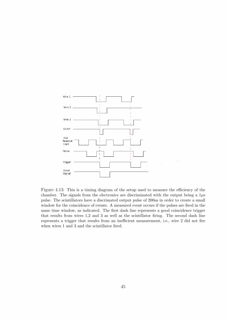
Figure 4.13: This is a timing diagram of the setup used to measure the efficiency of thechamber. The signals from the electronics are discriminated with the output being a 1µspulse. The scintillators have a discrimated output pulse of 200ns in order to create a smallwindow for the coincidence of events. A measured event occurs if the pulses are fired in thesame time window, as indicated. The first dash line represents a good coincidence triggerthat results from wires 1,2 and 3 as well as the scintillator firing. The second dash linerepresents a trigger that results from an inefficient measurement, i.e., wire 2 did not firewhen wires 1 and 3 and the scintillator fired.
45

Figure 4.14: This photo illustrates the testing setup including the use of the MAD card.Instead of signals being discriminated using NIM discriminators, the signals were discrimi-nated by the preamp/discriminator of the MAD card. This decreases the chance of pickingup noise in the signals and therefore decreases the uncertainty in our measurements.
Emitter coupled logic (ECL) signals from the MAD chip were sent to a Lecroy (Model
4616) ECL to NIM module which converted the signals to a useable NIM logic. The
same coincidence circuitry was used as before. In addition to the antenna to take
care of noise, a monitor wire, which consisted of a wire further away from the wires
that were being observed, was used. The idea behind this monitor wire is that only
the 3 sense wires should be fired as a track passes through the chamber. Therefore,
if this monitor wire fires in coincidence with the 3 sense wires, it is understood that
this event is not a true cosmic track and the signal should be ignored.
Preliminary measurements were made using the MAD preamp/discriminator
chip, (see Table 4.5 and Table 4.6) however, it was still unclear whether real events
were being observed. These efficiency measurements consisted of data from both
cosmic rays and the 90Sr source. The efficiencies were then plotted as a function of
46

high voltage; see Figure 4.15. In other attempts of trying to maximize the efficiency,
different variables were changed. The threshold on the MAD chip was constantly
adjusted because it was unsure what value this should be set at. The scintillators
were repositioned at different locations on the chamber in attempt to maximize the
efficiency. Copper plates were added above and below the MAD card in attempt
to shield the MAD chip from any noise that may affect measurements, Figure 4.16.
However, after several attempts, the efficiency seemed to fall below the desired and
expected value of 99%. Yet, the uncertainty that the chamber was still “picking” up
noise as well as the chamber was not at the operating voltage remained. However,
pushing the voltages higher was not possible since values of current were too dangerous
for the chamber.
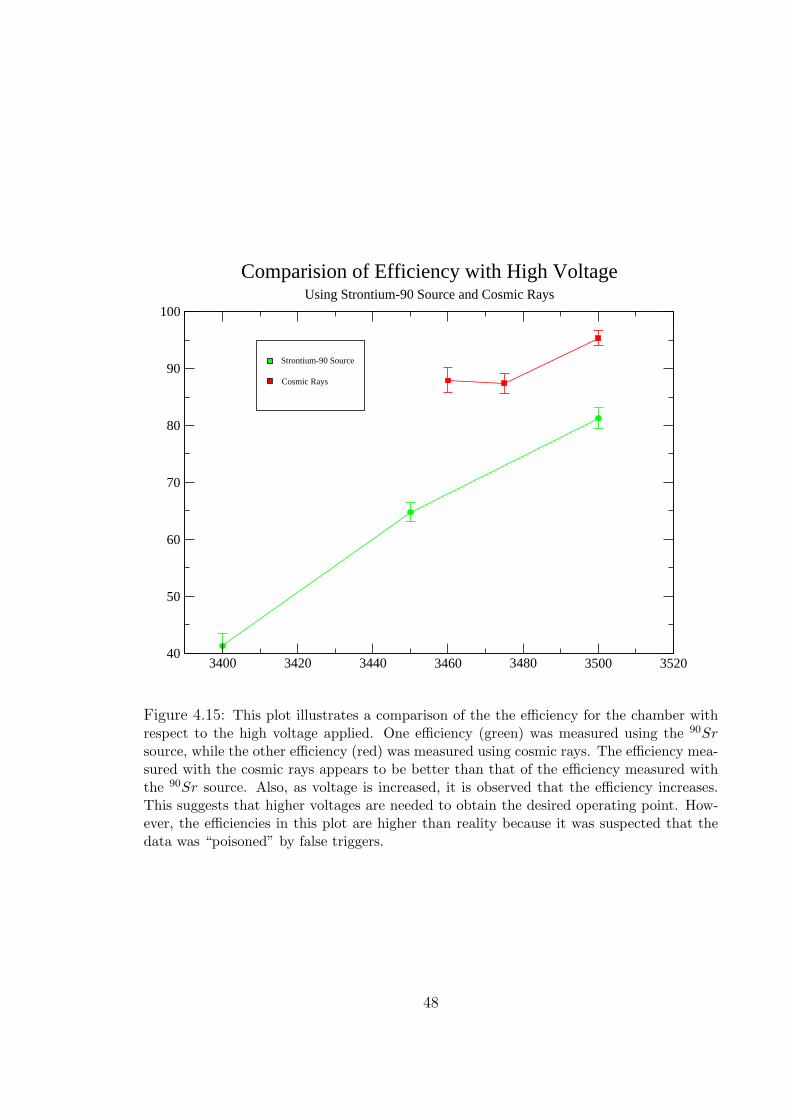
Voltage (kV) Wire Rate Efficiency3400 207/501 (41.3 ± 2.2)%3450 579/893 (64.8 ± 1.6)%3500 360/443 (81.3 ± 1.9)%
Table 4.5: This data table contains the measured wire rates and efficiency at a particularvoltage while using the 90Sr source. It was observed that the wire efficiency increased asthe voltage was increased.
Voltage (kV) Wire Rate Efficiency3460 189/215 (87.9 ± 2.2)%3475 244/279 (87.4 ± 1.8)%3500 243/255 (95.3 ± 1.3)%
Table 4.6: This data table contains the measured wire rates and efficiency at a particularvoltage while using cosmic rays. It was observed that the wire efficiency increased as thevoltage was increased.
47
3400 3420 3440 3460 3480 3500 352040
50
60
70
80
90
100
Comparision of Efficiency with High VoltageUsing Strontium-90 Source and Cosmic Rays
Strontium-90 Source
Cosmic Rays
Figure 4.15: This plot illustrates a comparison of the the efficiency for the chamber withrespect to the high voltage applied. One efficiency (green) was measured using the 90Sr
source, while the other efficiency (red) was measured using cosmic rays. The efficiency mea-sured with the cosmic rays appears to be better than that of the efficiency measured withthe 90Sr source. Also, as voltage is increased, it is observed that the efficiency increases.This suggests that higher voltages are needed to obtain the desired operating point. How-ever, the efficiencies in this plot are higher than reality because it was suspected that thedata was “poisoned” by false triggers.
48
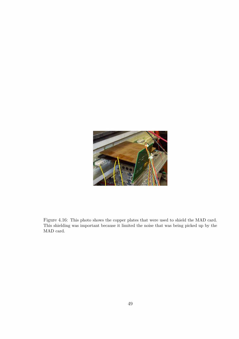
Figure 4.16: This photo shows the copper plates that were used to shield the MAD card.This shielding was important because it limited the noise that was being picked up by theMAD card.
49

It appeared that this first chamber would require more diagnostic work before
understanding the properties of the chamber. Since higher voltages could not be
applied to the chamber due to the spiking current, it was decided to pinpoint where
in the chamber the current was coming from. To do this, an ammeter was connected
to each individual readout card on the top and bottom wire frames and the current
was measured with a voltage of 3480V. The total current drawn by the chamber
at this voltage was 38µA, with 36.3µA being drawn from the bottom chamber and
0.4µA from the top. A plot of the currents drawn by each readout card was made
(Figure 4.17). Most of the current was being drawn from the bottom wire frame, with
11th readout card drawing the most current on this bottom frame. It was thought
that the cause for the bottom wire frame drawing the most current could be due
to height or separation distance variations in the individual wires along this frame.
However, instead of spending more time diagnosing the problem with this wire frame,
we decided to replace the wire frame with another, which required the chamber to be
disassembled. Testing of the chamber with this new wire frame in place will resume
after the chamber is reassembled.
4.1 Conclusions and Future Plans
Although many problems were encountered while trying to measure an efficiency
of the chamber, much had been learned. First, the bubbler effectively administers
the gas mixture to the chamber, without allowing any outside gas to enter. With a
broken or missing wire, the chamber is not able to reach the voltages that it should
because the chamber draws large amounts of current. It was confirmed with the
GARFIELD simulations that the cause of this resulted from large electric fields be-
tween the adjacent wires of the broken wire. For these Vertical Drift Chambers, it is
believed, when using the Argon/Ethane/CO2 gas mixture, that the operating voltage
50
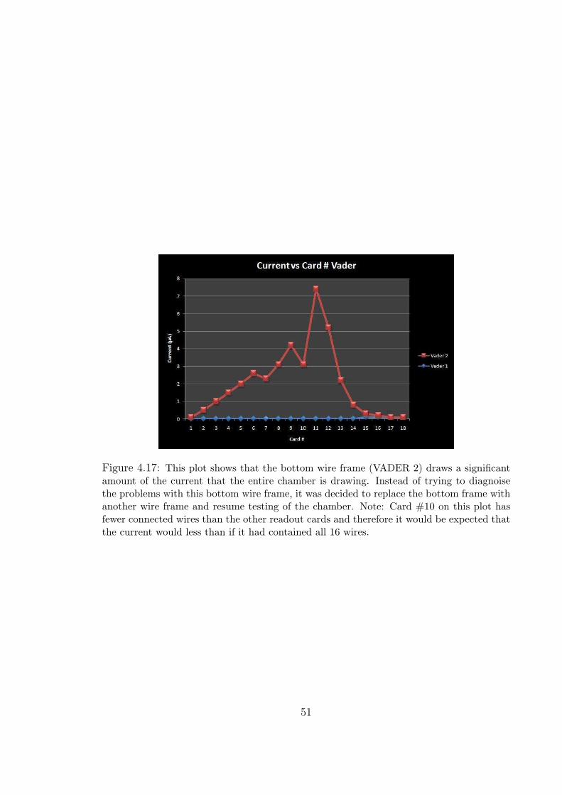
Figure 4.17: This plot shows that the bottom wire frame (VADER 2) draws a significantamount of the current that the entire chamber is drawing. Instead of trying to diagnoisethe problems with this bottom wire frame, it was decided to replace the bottom frame withanother wire frame and resume testing of the chamber. Note: Card #10 on this plot hasfewer connected wires than the other readout cards and therefore it would be expected thatthe current would less than if it had contained all 16 wires.
51
is near 3.4kV. Also, in order to properly condition the chamber, it takes roughly 24-48
hours of applying high voltages (in step increments). The chamber does see different
cosmic rays and events related to the 90Sr source. The MAD card works properly;
however, it is important to shield this card since it is sensitive to background noise in
the laboratory. An efficiency of the chamber was not able to be measured precisely
due to problems that were experienced with noise in the electronics and the currents
drawn by the chamber.
In terms of future work, there is still quite a bit of work left to complete. With
the wire frame replaced, the chamber will need to be reassembled and conditioned,
which should be completed within a week. During conditioning, higher voltages will
be tested in order to see if the current drawn by the chamber has decreased. It
is hoped that the current will decrease so that higher voltages can be used when
measuring the efficiency of the chamber. After conditioning, the efficiency of the
chamber will be tested in the same way, using cosmic rays and the 90Sr source. Once
the efficiency of the chamber has been measured and it is at or near 100% efficiency,
construction of the next chamber will take place and the process of conditioning and
measuring the efficiency will be repeated until all 5 vertical drift chambers have been
constructed, tested and characterized.
52

53
Bibliography
[1] B.R. Martin, G. Shaw. Particle Physics. John-Wiley and Sons Ltd, 1992. Ch.
8. pp 192-230.
[2] Rudolf Janoschek, Chirality- From Weak Bosons to the- Helix.
Springer-Verlag, 1991. pp 2-12.
[3] G.H. Wagniere. On Chirality and the Universal Asymmetry, Reflections on
Image and Mirror Image. VHCA, 2007. pp 24-27.
[4] L.H. Ryder. Elementary Particles and Symmetries. Gordon and Breach Science
Publishers, 1986. pp. 136-140.
[5] W.T.H. Van Oers, The Qweak Experiment: a Search for New Physics at the
TeV Scale. Nucl. Phys. 805. 2008. 329c-337c.
[6] Armstrong et al. The Qweak Experiment: A Search for New Physics at the
TeV Scale Via the Measurement of the Protons Weak Charge.
http://www.jlab.org/qweak/. 2001. (Unpublished; Proposal to Jefferson Lab
Program Advisory Committee).
[7] Brian P. Walsh. W&M Senior Thesis Project: “Development of a Flatness
Scanner and Simulation for Qweak Wire Chambers”. 2007. (Unpublished)
[8] W. Blum, L. Rolandi. Particle Detection with Drift Chambers.
Springer-Verlag. 1994. pp 1-8.
54
[9] S.C. Bennett and C.E. Wieman, Phys. Rev. Lett. 82, 2484 (1999); C.S.Wood,
et al., Science 275, 1759 (1997).
[10] P.L. Anthony, et al., (SLAC E158 Collaboration), Phys. Rev. Lett. 95, 081601
(2005).
[11] G.P. Zeller, et al., (NuTeV Collaboration), Phys. Rev. Lett. 88, 091802 (2002).
[12] Veenhof, Rob. “Garfield, a drift-chamber simulation program User’s Guide,
Version 4.29”.
http://www.slac.stanford.edu/comp/physics/cernlib/cerndoc/garfield.ps.gz.
Version 4.29. 30 Nov 1993.
55