Holger Kraft - Claus Munk - Frank Thomas Seifried - Sebastian Wagner

Consumption Habits and Humps SAFE Working Paper Series No. 15

Consumption Habits and Humps

Holger Krafta Claus Munkb Frank Thomas Seifriedc Sebastian Wagnerd

June 23, 2013

Abstract: We show that the optimal consumption of an individual over the life cycle

can have the hump shape (inverted U-shape) observed empirically if the preferences of

the individual exhibit internal habit formation. In the absence of habit formation, an

impatient individual would prefer a decreasing consumption path over life. However,

because of habit formation, a high initial consumption would lead to high required

consumption in the future. To cover the future required consumption, wealth is set aside,

but the necessary amount decreases with age which allows consumption to increase in

the early part of life. At some age, the impatience outweighs the habit concerns so

that consumption starts to decrease. We derive the optimal consumption strategy in

closed form, deduce sufficient conditions for the presence of a consumption hump, and

characterize the age at which the hump occurs. Numerical examples illustrate our

findings. We show that our model calibrates well to U.S. consumption data from the

Consumer Expenditure Survey.

Keywords: Consumption hump, life-cycle utility maximization, habit formation,

impatience

JEL subject codes: D91, D11, D14

a Department of Finance, Goethe University Frankfurt am Main, Faculty of Economics and Business Administra-tion, Germany. E-mail: holgerkraft@finance.uni-frankfurt.de

b Department of Finance, Copenhagen Business School, Denmark. E-mail: cm.fi@cbs.dkc Department of Mathematics, University of Kaiserslautern, Germany. E-mail: seifried@mathematik.uni-kl.ded Department of Finance, Goethe University Frankfurt am Main, Faculty of Economics and Business Administra-

tion, Germany. E-mail: Sebastian.Wagner@hof.uni-frankfurt.de

We appreciate comments from Nicola Fuchs-Schundeln, Michael Haliassos, and Mirko Wiederholt. Kraft andWagner gratefully acknowledge financial support by Deutsche Forschungsgemeinschaft (DFG).

Consumption Habits and Humps

Abstract: We show that the optimal consumption of an individual over the life cycle

can have the hump shape (inverted U-shape) observed empirically if the preferences of

the individual exhibit internal habit formation. In the absence of habit formation, an

impatient individual would prefer a decreasing consumption path over life. However,

because of habit formation, a high initial consumption would lead to high required

consumption in the future. To cover the future required consumption, wealth is set aside,

but the necessary amount decreases with age which allows consumption to increase in

the early part of life. At some age, the impatience outweighs the habit concerns so

that consumption starts to decrease. We derive the optimal consumption strategy in

closed form, deduce sufficient conditions for the presence of a consumption hump, and

characterize the age at which the hump occurs. Numerical examples illustrate our

findings. We show that our model calibrates well to U.S. consumption data from the

Consumer Expenditure Survey.

Keywords: Consumption hump, life-cycle utility maximization, habit formation,

impatience

JEL subject codes: D91, D11, D14

1 Introduction

Empirical studies have documented that the consumption expenditures of individuals typically have

an inverted U-shape over the life cycle by being increasing up to age 45-50 years and then decreasing

over the remaining life. Standard, frictionless consumption-savings model cannot generate such a

hump in consumption: if the subjective time preference rate of the individual is higher [lower] than

the (risk-adjusted expected) return on investments, consumption is expected to decrease [increase]

monotonically over the entire life time. Several plausible models that lead to a consumption hump

have been suggested (see below), but these models are relatively complex and can only be solved

with the help of numerical methods. This paper shows that, even in a very simple setting, the

consumption hump can naturally emerge when the preferences of the individual exhibit habit

formation instead of the time-additivity typically assumed.

The hump in life-cycle consumption emerges from a trade-off between impatience and the impli-

cations of habits. Suppose the individual has a high subjective time preference rate and thus, other

things equal, would prefer to have a decreasing consumption pattern over life. However, if the in-

dividual forms enduring habits for consumption, she knows that a high initial consumption would

lead to higher required consumption in the future. Consequently, she trades off the impatience

regarding current consumption with the concerns about the future required consumption levels

resulting from habit formation. The younger the individual, the more money has to be set aside to

cover future required consumption. A sufficiently strong habit formation dominates the impatience

in the early years, but as habit concerns decrease over life consumption gradually increases in the

early years. At some age, the impatience outweighs the habit concerns so that consumption starts

to decrease. Hence, the consumption pattern over the life cycle exhibits a hump.

The tradeoff between impatience and habit formation is fundamental, and we illustrate it in

the simplest possible model with full certainty and no frictions. The individual is equipped with

some initial wealth that can be invested at a constant risk-free rate. The individual can continu-

ously withdraw funds for consumption. We assume that the individual’s objective is to maximize

utility of consumption over the remaining life. The utility at a given point in time is a concave

power function of the difference between consumption and the habit level at that time, where the

habit level is a scaled, exponentially weighted average of past consumption rates of the individual.

This standard specification of habit-style preferences implies that the habit level is the minimum

feasible consumption and, therefore, the individual must ensure to have sufficient funds to cover

1

the minimum feasible consumption in the remaining life. This generates required savings which

are, other things equal, decreasing as the remaining life-time shrinks.

The optimal consumption profile and the possibility of a hump in consumption depend on the

values of various parameters of the model. We derive a set of sufficient conditions for the presence

of a consumption hump. For a reasonable parametrization of the model, we show that the optimal

consumption profile of the agent does exhibit a hump and that the consumption hump occurs at an

age consistent with the empirical evidence. We illustrate how the location of the hump is affected

by the various parameters in a way consistent with economic intuition. For example, we find that

the bigger the impact of current consumption on future habit levels (via a higher scaling parameter

and a lower decay rate of the habit level), the later the consumption hump occurs. Moreover,

consumers who are very impatient or very risk-tolerant (i.e., consumers having a high elasticity of

intertemporal substitution) have a consumption profile peaking at a relatively young age.

We calibrate our model to consumption data from the Consumer Expenditure Survey in the

United States over the period 1980-2003. We find that our model matches very well the observed

hump-shaped consumption pattern of both singles and couples.

The habit formation we model is sometimes referred to as internal habit formation to emphasize

that the habit level entering the utility function is a result of the past consumption choices of the

same individual. This can be contrasted with the case of subsistence consumption in which the

individual derives utility from consumption above some exogenously given subsistence level and also

to the case of external habit formation in which the individual’s utility of consumption depends on

some external factor, e.g., the consumption choices of peers (“keeping up with the Jones’es”) or

the per capita consumption in the economy.

The rest of the paper is organized as follows. Section 2 reviews the related literature. Section 3

presents the model and provides a closed-form solution for the optimal consumption plan. Analyt-

ical results on the existence and location of the consumption hump are demonstrated in Section 4.

Section 5 illustrates the optimal consumption profile for a set of benchmark parameter values and

discusses the sensitivity with respect to the values of key parameters. Section 7 concludes. Proofs

can be found in the appendices.

2

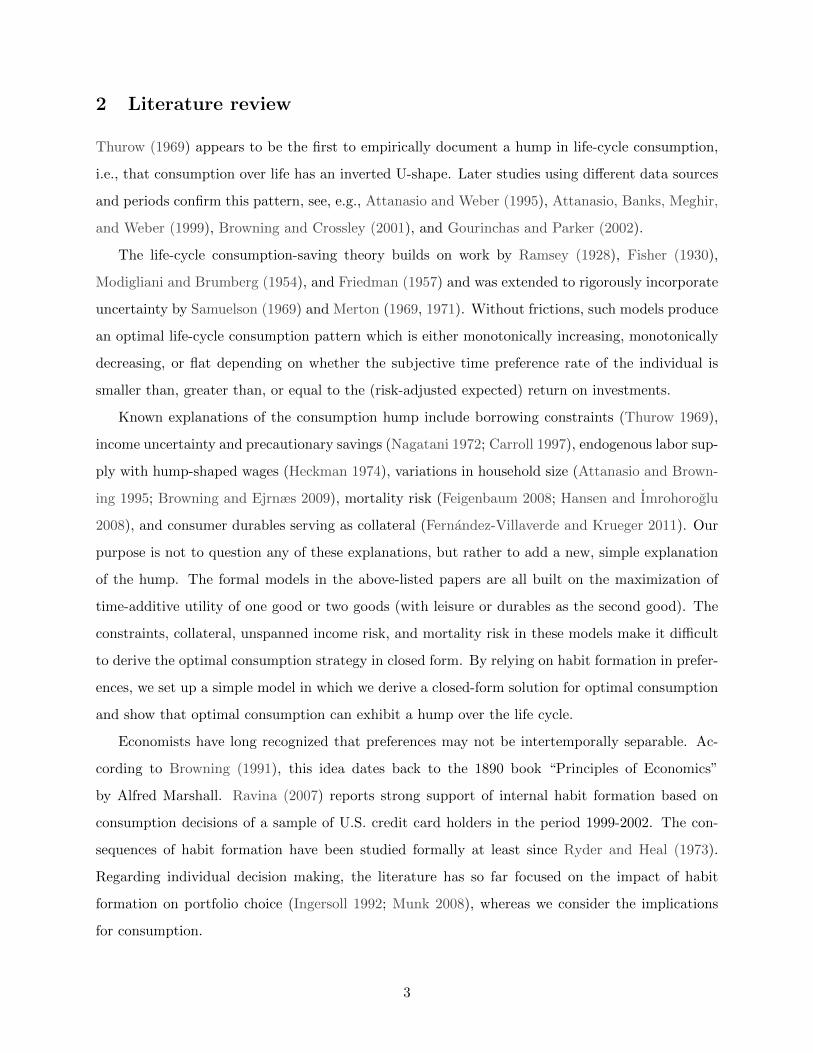
2 Literature review

Thurow (1969) appears to be the first to empirically document a hump in life-cycle consumption,

i.e., that consumption over life has an inverted U-shape. Later studies using different data sources

and periods confirm this pattern, see, e.g., Attanasio and Weber (1995), Attanasio, Banks, Meghir,

and Weber (1999), Browning and Crossley (2001), and Gourinchas and Parker (2002).

The life-cycle consumption-saving theory builds on work by Ramsey (1928), Fisher (1930),

Modigliani and Brumberg (1954), and Friedman (1957) and was extended to rigorously incorporate

uncertainty by Samuelson (1969) and Merton (1969, 1971). Without frictions, such models produce

an optimal life-cycle consumption pattern which is either monotonically increasing, monotonically

decreasing, or flat depending on whether the subjective time preference rate of the individual is

smaller than, greater than, or equal to the (risk-adjusted expected) return on investments.

Known explanations of the consumption hump include borrowing constraints (Thurow 1969),

income uncertainty and precautionary savings (Nagatani 1972; Carroll 1997), endogenous labor sup-

ply with hump-shaped wages (Heckman 1974), variations in household size (Attanasio and Brown-

ing 1995; Browning and Ejrnæs 2009), mortality risk (Feigenbaum 2008; Hansen and Imrohoroglu

2008), and consumer durables serving as collateral (Fernandez-Villaverde and Krueger 2011). Our

purpose is not to question any of these explanations, but rather to add a new, simple explanation

of the hump. The formal models in the above-listed papers are all built on the maximization of

time-additive utility of one good or two goods (with leisure or durables as the second good). The

constraints, collateral, unspanned income risk, and mortality risk in these models make it difficult

to derive the optimal consumption strategy in closed form. By relying on habit formation in prefer-

ences, we set up a simple model in which we derive a closed-form solution for optimal consumption

and show that optimal consumption can exhibit a hump over the life cycle.

Economists have long recognized that preferences may not be intertemporally separable. Ac-

cording to Browning (1991), this idea dates back to the 1890 book “Principles of Economics”

by Alfred Marshall. Ravina (2007) reports strong support of internal habit formation based on

consumption decisions of a sample of U.S. credit card holders in the period 1999-2002. The con-

sequences of habit formation have been studied formally at least since Ryder and Heal (1973).

Regarding individual decision making, the literature has so far focused on the impact of habit

formation on portfolio choice (Ingersoll 1992; Munk 2008), whereas we consider the implications

for consumption.

3

Habit features in preferences have proven helpful in explaining stylized asset pricing facts that

seem puzzling when agents are assumed to have time-separable power utility, see, e.g., Sundaresan

(1989), Abel (1990), Constantinides (1990), Campbell and Cochrane (1999), and Menzly, Santos,

and Veronesi (2004). Based on an endowment economy with identical agents, Grischenko (2010)

concludes that an internal habit specification provides a better match with asset pricing data than

an external habit specification. Heaton (1995) and Chen and Ludvigson (2009) report similar

results. Habit formation is also used in other areas of macroeconomics, see, e.g., Carroll, Overland,

and Weil (2000), Boldrin, Christiano, and Fisher (2001), and Del Negro, Schorfheide, Smets, and

Wouters (2007). Fuhrer (2000) and Christiano, Eichenbaum, and Evans (2005) show that habit

formation may explain the hump-shaped response over time of aggregate consumption to a monetary

policy shock. In contrast, we show that habit formation may lead to (expected) consumption being

hump-shaped over the life of an individual.

3 The model

We set up a deterministic, continuous-time model of an individual’s life-cycle consumption and

savings decisions. The individual enters the economy at time 0 with some initial wealth X0 and

lives until time T > 0, which we assume is a known constant. The individual consumes a single

consumption good with c(t) representing the consumption rate at time t, so that the number of

goods consumed over a short interval [t, t+ dt] is approximately c(t) dt. The good is the numeraire

in the economy. The wealth not spent on consumption is invested in a savings account that offers

a constant, risk-free rate of r, continuously compounded. The individual receives no other income

during life than the interest on savings. The dynamics of wealth X(t) is then simply

dX(t) = rX(t) dt− c(t) dt. (1)

The individual has to determine a consumption strategy (c(t))t∈[0,T ], which in our deterministic

setting is simply a function c : [0, T ] 7→ R.

We assume that the preferences of the individual exhibit (internal) habit formation. We define

the time t habit level to be

h(t) = h0e−βt + α

∫ t

0e−β(t−s)c(s) ds, (2)

4

where h0, α, and β are non-negative constants. The last term is proportional to a weighted average

of past consumption where we can interpret β as a persistence parameter and α as a scaling

parameter. Finally, h0 ≥ 0 is an initial habit level whose influence fades away over time provided

that β > 0. Note that the habit level evolves as

dh(t) = (αc(t)− βh(t)) dt. (3)

Given a wealth of x and a habit level of h at time t, the individual is assumed to evaluate a

given consumption strategy c = (c(s))s∈[t,T ] over the remaining life by

Jc(t, x, h) =

∫ T

te−δ(s−t)U (c(s)− h(s)) ds+ εe−δ(T−t)U (X(T )) , (4)

where δ is a constant subjective time preference rate, ε ≥ 0 is a constant indicating the preference

weight of the bequest XT relative to consumption, and

U(z) =1

1− γz1−γ (5)

where γ > 1 is a risk aversion parameter. The relative risk aversion with respect to consumption

gambles is −c∂2U(c−h)∂c2

/∂U(c−h)∂c = γc/(c−h) so that γ is the minimal relative risk aversion possible.

The indirect utility function is defined as

J(t, x, h) = maxcJc(t, x, h). (6)

As we want to illustrate in the simplest possible setting that habit formation can induce a consump-

tion habit, we deliberately assume full certainty in our model. Hence, the concept of risk aversion

may seem misplaced, but we can alternatively think in terms of the elasticity of intertemporal

substitution, which is the reciprocal of the relative risk aversion, i.e., (c− h)/(γc). A higher γ rep-

resents a lower elasticity of intertemporal substitution and 1/γ is the maximal level of the elasticity

of intertemporal substitution.1 For terminological convenience we will continue to refer to γ as a

risk aversion parameter in the remainder of the paper.

The setup requires that consumption stays above the habit level, otherwise the marginal utility

1An alternative measure of the elasticity of intertemporal substitution is the derivative of the consumption growthrate with respect to the interest rate. The two measures are identical in the setting without habit formation, but notin the setting with habit formation as explained by Constantinides (1990) in the case of an infinite time horizon.

5

would be infinite. This implies that wealth at any point in time has to be sufficient to finance

future minimum consumption. If the individual has a time t habit level of h(t) and consumes at

the minimum level (i.e., habit level) in all future so that c(s) = h(s), the habit level evolves as

dh(s) = −(β − α)h(s) ds which implies that

h(s) = e−(β−α)(s−t)h(t), s ∈ [t, T ].

The time t present value of this stream of minimum future consumption is

∫ T

te−r(s−t)h(s) ds = h(t)A(t),

where

A(t) =

T − t, if rA = 0,

1

rA

(1− e−rA(T−t)

), otherwise,

(7)

with

rA = r + β − α.

Remark 1. It seems natural to expect that β > α since then the habit level decreases whenever the

agent consumes at the minimum level as can be seen by applying c(t) = h(t) in (3). If, furthermore,

the interest rate is non-negative, the constant rA is definitely positive.

Intuitively, the individual can split up her time t wealth into tied-up wealth h(t)A(t), which

covers the minimum future consumption, and the free wealth X(t) − h(t)A(t) which can finance

excess consumption and thus generates utility. This explains the form of the solution to the utility

maximization problem. The following theorem gives the exact formulation. See Appendix A for a

proof.

Theorem 1. Assume x > hA(t). Then the indirect utility function is given by

J(t, x, h) =1

1− γg(t)γ(x− hA(t))1−γ , (8)

6

where A is given by (7) and

g(t) =

∫ T

te−rg(s−t)(1 + αA(s))

γ−1γ ds+ ε

1γ e−rg(T−t), (9)

rg =γ − 1

γr +

δ

γ.

The optimal consumption strategy is

c(t) = h(t) +X(t)− h(t)A(t)

g(t)(1 + αA(t))

− 1γ . (10)

In the following, we are mainly interested in the shape of the function t 7→ c(t).

Let us briefly consider some special cases. First, consider the case with constant relative risk

aversion which requires h0 = α = β = 0. In this case optimal consumption is simply c(t) =

X(t)/g(t) and, since X ′(t) = (r − g(t)−1)X(t) and g′(t) = rgg(t)− 1, we obtain

c′(t) =(r − rg)X(t)

g(t)=r − δγ

X(t)

g(t). (11)

Hence, we see that the consumption function is increasing if r > δ (the return on savings exceeds

the impatience), decreasing if r < δ, and flat if δ = r. Secondly, consider the case where the

consumption benchmark h(t) is an exogenously given function (an external habit or a subsistence

consumption level) and, in particular, α = 0 so that consumption does not affect future values

of h(t). In this case optimal consumption becomes

c(t) = h(t) +X(t)− F (t)

g(t), F (t) =

∫ T

te−r(s−t)h(s) ds, (12)

where g is given by (9) albeit with α = 0 and we must require X(t) > F (t). Then

c′(t) = h′(t) +r − δγ

X(t)− F (t)

g(t), (13)

which is decreasing if h is decreasing and δ > r, but can be increasing under other assumptions.

With a suitably specified benchmark function h(t), the optimal consumption path can even exhibit

a hump.

Now we return to the case with (internal) habit formation. Note that direct differentiation with

respect to time in (10) would involve the derivatives of both h(t) and X(t), but the latter can be

7

expressed in terms of X(t) and c(t) through (1) and then the X(t) can be expressed in terms of

c(t) and h(t) using (10). Hence, the derivative of c(t) can be expressed in terms of c(t) and h(t).

From (3), the derivative of h(t) can be expressed in terms of c(t) and h(t). In fact, it turns out to

be useful to rewrite the system of derivatives of c(t) and h(t) as a system of derivatives of c(t) and

the surplus consumption defined as

∆(t) = c(t)− h(t). (14)

Note that the optimal consumption strategy is such that the surplus consumption is a time-

dependent fraction of the free wealth. We summarize the derivatives in the following theorem,

which is proved in Appendix B.

Theorem 2. The dynamics of the optimal consumption and the associated surplus consumption is

given by the system

d∆(t) = φ(t)∆(t) dt, (15)

dc(t) = (β + φ(t)) ∆(t) dt− (β − α) c(t) dt, (16)

where

φ(t) =r − δ + αB(t)

γ, (17)

B(t) =1− rAA(t)

1 + αA(t)=

1

1 + α(T − t), if rA = 0,

rA(rA + α)erA(T−t) − α

, otherwise.(18)

In the next section we provide analytical results on the existence and location of a hump in the

consumption function t 7→ c(t). Section 5 illustrates the results by numerical examples.

4 Analytical results on the consumption hump

While the expression (10) for optimal consumption appears simple, note that it depends both on

h(t), which is determined by the entire consumption path up to time t via (2), and on wealth, which

also is determined by past consumption via (1). In general it seems very difficult to analytically

establish conditions under which consumption is hump-shaped.

8

For long horizons, however, we can obtain an analytical characterization of the consumption

pattern and establish sufficient conditions for the existence of a consumption hump. As explained

in the introduction, the hump emanates from a combination of habit formation and an impatience

exceeding returns on savings. In light of Remark 1, the following assumption is therefore natural.

Assumption 1. The parameters satisfy the conditions δ > r, α > 0, and rA = r + β − α > 0.

Recall that the condition δ > r requires the agent to be sufficiently impatient so that the

consumption in the absence of habit formation would be monotonically decreasing over life. The

condition α > 0 means that the habit level is increasing in past consumption so that preferences

exhibit genuine habit formation.

With α > 0, it is clear from (17) and (18) that both B(t) and φ(t) smoothly approach constants

as the terminal time T is increased. For T large enough, the graph of φ(t) is almost flat in the

early years. With rA > 0, the limit of φ(t) as T →∞ is (r − δ)/γ. Define the constant

κ =δ − rγ

,

which can be interpreted as the product of a net impatience rate δ − r and the maximal elasticity

of intertemporal substitution 1/γ. By Assumption 1, we have κ > 0. We now replace φ(t) in the

true dynamics (15) of the surplus consumption with its limit (r− δ)/γ = −κ and thus consider the

time-independent dynamics

d∆(t) = −κ∆(t) dt, (19)

dc(t) = (β − κ)∆(t) dt− (β − α)c(t) dt (20)

with initial values c0 > ∆0 > 0. We demonstrate in numerical examples in Section 5 that the

time-independent dynamics (19)–(20) is an accurate approximation of the true dynamics (15)–(16)

except possibly for the final years. See also Lemma 1 below.

The next theorem establishes conditions under which the approximating dynamics produce a

unique hump in the function c(t). Appendix C provides the proof.

Theorem 3. Suppose Assumption 1 is satisfied and that

β > α+ κ, (21)

(α− κ)c0 > (β − κ)h0, (22)

9

where h0 = c0 − ∆0. Then the solution to the dynamic system (19)–(20) is such that the function

c(t) has a unique hump at t = tH , where

tH =ln(β − α)− ln(κ) + ln

(1− c0

λ(c0−h0)

)β − α− κ

, (23)

and where

λ =β − κ

β − α− κ. (24)

We emphasize that the parameter conditions stated in Theorem 3 are sufficient, not necessary,

for the presence of a hump.

The condition (21) requires the decay rate β of the habit to be sufficiently high so that the habit

is not too persistent. Note that κ > 0 since δ > r, so the condition (21) sharpens the inequality

β > α which is natural, cf. Remark 1. If we assume α > κ and c0 = c0, the inequality (22) can be

rewritten, by applying (10) at t = 0, as

X0 >

(A(0) +

β − αα− κ

g(0)(1 + αA(0))1/γ)h0,

so that it is satisfied for a large enough initial wealth. Note that the parameter conditions stated

in the theorem ensure that the log-terms in (23) are well-defined.

The hump derived from the approximate dynamics occurs at age tH . Note that, for fixed initial

values c0 and h0, tH is independent of the horizon T of the agent. This observation highlights that

the above theorem is relevant for the hump in the truly optimal consumption path if the horizon

is sufficiently large and, in particular, larger than tH . We find that tH is increasing in c0. Holding

c0 fixed, we find that tH is increasing in r, γ, and α, but decreasing in h0, δ, and β.

The following lemma shows that we can bound the difference between the true consumption

function and the approximation over any interval [0, t] by any margin η > 0 if the planning horizon

T is long enough. The proof can be found in Appendix D.

Lemma 1. Suppose Assumption 1 and the conditions (21) and (22) hold. Let h0 = h0 and c0 = c0.

For any given t ≥ 0 and any given η > 0, we can find T > 0 such that if T > T then

|c(s)− c(s)| < η, s ∈ [0, t]. (25)

By applying the lemma for t > tH and a small η, we see that the true dynamics also give rise

10

to a consumption hump if the stated parameter conditions are satisfied and the horizon T is long

enough.

In Section 5 we show in numerical examples that the approximate dynamics is very close to the

true dynamics over most of life even for realistic horizons, and we therefore also see a consumption

hump in such cases.

5 Numerical examples

In the following numerical examples we use the benchmark parameter values listed in Table 1 unless

otherwise mentioned. We assume the agent has a remaining time horizon of 50 years, so the setting

could represent the problem faced by an agent who is initially 30 years old and who lives until an

age of 80. The agent has no utility of bequests.2 The initial wealth is set to X0 = 20 which is

motivated by the observation that the median wealth for individuals of age 30-40 in the 2007 Survey

of Consumer Finances is roughly USD 20,000. The benchmark values of the interest rate, the time

preference rate, and the risk aversion parameter fall in the range considered in the literature. The

initial value of the relative risk aversion γc0/(c0 − h0) turns out to be around 9. The initial habit

level is set at 0.25 which, compared to the initial consumption level that turns out to be 0.45,

represents a significant but not extremely strong habit; the initial consumption is approximately

44% above the minimum consumption level which is identical to the habit level. The values of

the habit parameters α and β are less clear given the limited literature. We consider values in the

range also studied by Constantinides (1990) and Munk (2008), which seem to generate reasonable

habit dynamics.

[Table 1 about here.]

Figure 1 illustrates the optimal consumption path with the benchmark parameter values. Con-

sumption exhibits a distinct hump with a maximum after 20.3 years, which could correspond to an

age of roughly 50 years, cf. the above discussion. This location of the hump matches well the em-

pirically observed hump. Based on the analytical approximation the hump time is tH ≈ 19.8 years,

very close to the actual time of the hump. We can see that the consumption pattern based on

the approximate, long-horizon dynamics (thin curve) is virtually indistinguishable from the actual

consumption pattern over the first 30 years. The consumption levels are unrealistically low as we

2This is in line with Hurd (1989) who shows empirically that bequest motives in various countries are close tozero.

11

do not take labor income into account, but a quick fix is to scale initial wealth appropriately to

incorporate human capital, which leads to a similar scaling of consumption levels (provided that

the initial habit level is scaled accordingly). This procedure does not affect the shape of the con-

sumption path, nor the presence and location of the hump. The habit level tracks the consumption

path closely.

Figure 1 further shows the monotonically decreasing consumption path of an agent not develop-

ing habits, but having a constant relative risk aversion (i.e., a constant elasticity of intertemporal

substitution). As explained below Theorem 1, this is a consequence of δ exceeding r so that im-

patience beats returns on savings. Note the dramatic impact habit formation has on the optimal

consumption path.

[Figure 1 about here.]

Next we investigate the sensitivity of the consumption path and the location of the consumption

hump with respect to the values of key parameters. Figure 2 shows the optimal consumption profile

for three different values of the habit scaling parameter α. Increasing α, current consumption has a

bigger effect on future habit levels, which leads the agent to lower consumption in the early years.

The increased savings are spent on higher consumption in the late years of life. Consequently, the

consumption hump occurs later in life. For very small values of α (in our case around 0.1 and

smaller), the consumption profile is monotonically decreasing over life (except for a small increase

in the final couple of years), as in the case without habits, since then the habit level does not have

a sufficient magnitude to subdue the impatience of the agent. Conversely, for very high values of α

(in our case around 0.35 and higher), the consumption profile is monotonically increasing.

[Figure 2 about here.]

Figure 3 illustrates the importance of the habit persistence parameter β. A higher β means

reduced influence of current consumption on future habit levels. Hence, the agent initially consumes

more, which is naturally offset by lower consumption late in life. A higher β therefore also leads

to an earlier consumption hump. If β is sufficiently high (around 0.85 and higher in our case), the

hump disappears and consumption monotonically decreases over life except for the few final years

where consumption increases. If β is sufficiently small (0.37 or lower), the optimal consumption is

monotonically increasing over life.

[Figure 3 about here.]

12

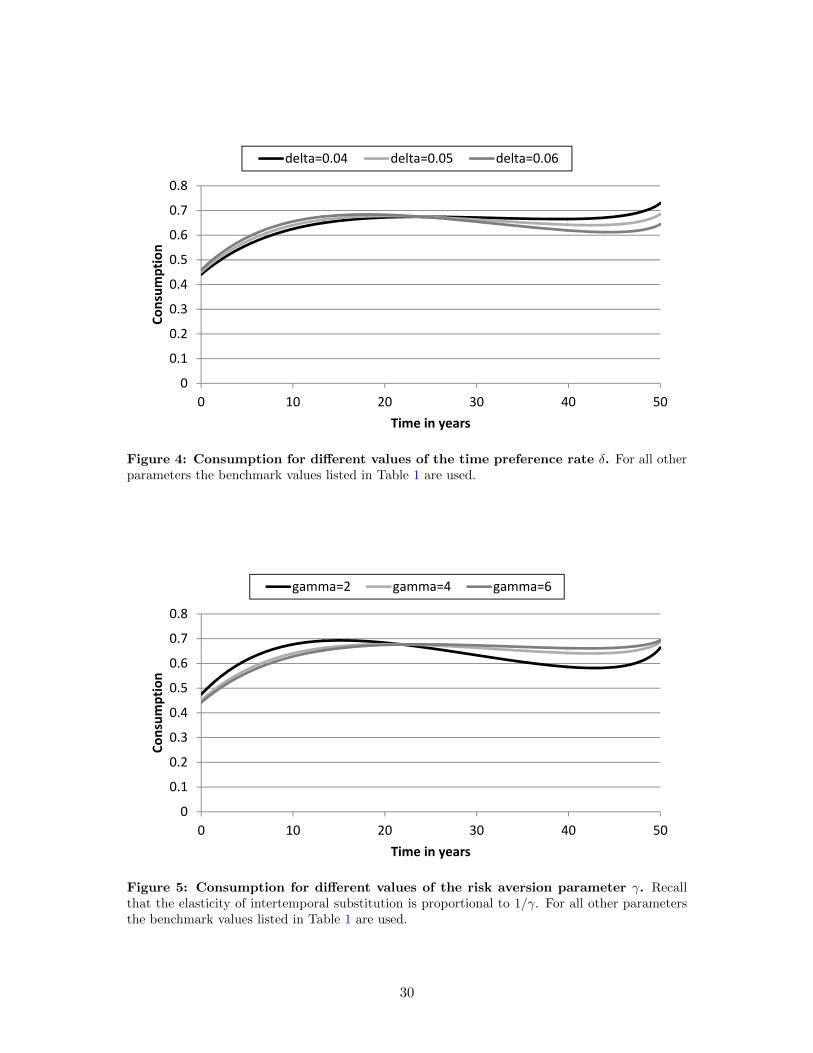
The role of the time preference rate δ can be seen in Figure 4. A higher δ means that the

agent is more impatient and therefore increases consumption early in life with the consequence of

reducing consumption late in life, which also causes the consumption hump to occur earlier in life.

Because a high early consumption raises the minimum consumption level in the following years,

it takes an extremely high value of δ (in our case 1.10 or higher) before the consumption path

becomes downward-sloping right from the beginning. For low values of δ (around 0.035 and lower),

the optimal consumption profile is monotonically increasing. Note that this happens also for cases

in which optimal consumption in the absence of habit formation is monotonically decreasing; in

our case this occurs for δ between 0.02 (the benchmark value of r) and 0.035.

[Figure 4 about here.]

Figure 5 shows that a higher value of the risk aversion parameter γ – or equivalently a lower

value of the elasticity of intertemporal substitution 1/γ – leads to lower consumption early in life

and higher consumption late in life with the consumption hump occurring later in life.

[Figure 5 about here.]

Figure 6 illustrates the optimal consumption profile for three different values of the time hori-

zon T . Since we fix the initial wealth and disregard labor income, the agent with a longer horizon

consumes at a lower level throughout life. The consumption hump occurs earlier for longer horizons.

For a sufficiently short horizon (about 42 years or shorter, given the other parameter values) the

consumption path is monotonically increasing over life.

[Figure 6 about here.]

Finally, we consider the relevance of the strength of the bequest motive as represented by the

parameter ε, cf. the preference specification in (4). We have used a benchmark value of ε = 0

corresponding to no utility of bequest, which obviously implies that the agent consumes everything

and ends up with zero wealth. In Figure 7 we compare the benchmark consumption profile with

the consumption profile when ε is either one thousand or one million. In the first of these two

cases, the agent leaves a bequest of 1.035 (compare with the initial wealth of 20) which corresponds

to roughly the consumption in the final 1.5 years. In the latter case, the agent leaves a bequest

of 5.294 corresponding to the consumption over the final 8-9 years. Naturally, we see that the

stronger the bequest weight ε, the lower the consumption throughout life as more savings need to

13

be generated. However, the shape of the consumption profile and the location of the consumption

hump are only affected slightly. The hump occurs after 20.3 years without bequest, after 20.1 years

when ε = 1000, and after 19.4 years when ε = 1000000.

[Figure 7 about here.]

An interesting observation from the figures presented above is that, after the mid-life hump and

subsequent decline, optimal consumption starts to increase again in the final years of life. However,

this behavior depends on the constellation of parameter values. Figure 8 shows an optimal con-

sumption path with no increase near the end, based on a set of reasonable parameter values. In this

particular case, the slope of the consumption path becomes less negative so that the consumption

path flattens out near the end. It appears to be impossible to provide a simple analytical charac-

terization of the shape of the optimal consumption path just before the terminal date. Intuitively,

as the terminal date approaches, the agent becomes less concerned about the impact of current

consumption on future habit levels as the future is becoming increasingly irrelevant. Therefore, the

dampening effect of internal habit formation on consumption weakens as the final date approaches.

Of course, even in the final years, the agent has to cope with the current minimum consumption

level caused by past consumption decisions. Therefore, the optimal consumption decision of the

agent with internal habit formation does not approach the optimal decision of an agent with con-

stant relative risk aversion, but rather the optimal consumption of an agent with an external habit

or subsistence consumption level. In the larger picture, the optimal consumption pattern (late) in

retirement is heavily influenced by the increase in mortality risk ignored by our simple model.

[Figure 8 about here.]

The key empirical papers documenting the hump consider consumption only up to about age 65,

and their graphs indicate that consumption flattens out in the years leading up to that age, cf., e.g.,

Figure 1 in Feigenbaum (2008). This appears consistent with the flattening of the consumption

path in the final years in our Figure 8 or with the relatively flat part of the consumption path in, say,

Figure 1 just before the final few years of increasing consumption. The limited existing empirical

evidence on consumption in retirement is inconclusive with respect to how consumption varies with

age late in retirement, cf., e.g., Fisher, Johnson, Marchand, Smeeding, and Torrey (2005).3

3In contrast, there is substantial empirical evidence that consumption typically falls at retirement, but this shouldbe seen in relation to frequently occurring contemporaneous changes in leisure, housing, health conditions, mortalityrisk, and household composition, cf., e.g., the discussion in Browning and Crossley (2001).

14

6 Calibrating the model to consumption data

In this section we investigate the extent to which our model can match the observed consumption

hump. We apply consumption data from the Consumer Expenditure Survey from the United States

over the period 1980-2003. The data was originally processed and used by Krueger and Perri (2006)

and it is made available online by the authors.4 The consumption is deflated back to represent

“1982-84 constant dollars.” We apply their so-called ND+ consumption measure; we refer the reader

to Krueger and Perri (2006) for details on the data. The consumption data is on a household basis,

whereas our model is better suited for individuals. We focus on the consumption of singles and

the per-person consumption of couples without children (household consumption divided by 1.7 as

recommended by the OECD equivalence scale). The uneven curves in Figure 9 show the average

consumption per year in thousands of US dollars for individuals at different ages who are living

either as singles (upper panel) or in childless couples (lower panel). The consumption of singles

is relatively flat over life, but still higher in mid-life than in the early and in the late years. The

consumption of couples exhibits a more pronounced hump-shape.

[Figure 9 about here.]

We calibrate our model so that the optimal consumption path from the model best matches

the observed age-profile of consumption of either singles or couples. Since the consumption data

covers ages from 25 to 65, we let t = 0 and T = 40. We fix the risk-free rate at r = 0.01 and

assume no utility from bequeathing wealth (ε = 0). We search for the remaining parameters with

the objective of minimizing the sum of the squared differences between the model consumption and

the observed average consumption at ages 25, 26, . . . , 65. Table 2 shows the parameter values from

the calibrations. The habit process parameters α and β have very reasonable values. We restrict

α to be at least 0.1, which is a binding constraint in the calibration to the consumption of singles.

As long as the difference β − α is fixed, we can also obtain an excellent fit to the data for higher

values of α and β. The time preference rate δ is restricted to be at most 0.25. A slightly better

fit can be obtained by increasing δ further (together with the risk aversion parameter γ). On the

other hand, we also obtain a good fit to the data if we lower both δ and γ (results are available on

request). When comparing the value of the initial wealth to real-life wealth levels, recall that the

model wealth includes any human capital.

4Web-link: http://www.fperri.net/research_data.htm

15

[Table 2 about here.]

The smooth curves in Figure 9 depict the life-cycle consumption pattern from our calibrated

model. The figure illustrates that our parsimonious model driven by impatience and habit for-

mation nicely matches the observed consumption pattern over the life-cycle including the mid-life

consumption hump. Our calibration is mostly challenged by the apparent substantial increase in

the consumption of persons of an age between, say, 30 and 45 years who live in a childless couple.

However, this pattern may be partially explained by a “survivorship” bias in the sample. Obvi-

ously, when the persons in a couple become parents, they leave this group of individuals and their

subsequent consumption is not reflected by the data we use. If the less wealthy and therefore low-

consuming couples are more inclined to become parents, the remaining sample of childless couples

is tilted towards the more wealthy and high-consuming individuals.

7 Conclusion

This paper proposes a new potential explanation of the empirically observed hump in the consump-

tion of individuals over their life cycle. If the preferences of the individual exhibit habit formation,

the hump can naturally materialize from a tradeoff between impatience and concerns about the

effects of current consumption on future habit levels and thus future minimum consumption. The

habit concerns cause a large reduction in the otherwise very high consumption early in life, but a

smaller reduction of the otherwise medium-sized consumption in mid life. In some circumstances,

a hump-shaped consumption path emerges.

We present a set of sufficient conditions for the presence of a hump and characterize the age at

which the hump occurs. Numerical examples illustrate the consumption hump and the sensitivity

of the optimal consumption path to the values of key parameters of our model. We show that our

parsimonious model provides a nice match with consumption patterns derived from the 1980-2003

Consumer Expenditure Surveys in the United States.

As the purpose of the paper is to demonstrate that habit formation can generate a consumption

hump, we deliberately keep our model simple and, in particular, disregard uncertainty, labor income,

portfolio constraints etc. However, the basic tradeoff identified in this paper carries over to more

elaborate settings.

16

A Proof of Theorem 1

The Hamilton-Jacobi-Bellman (HJB) equation associated with the utility maximization problem (6)

is

0 = maxc

{1

1− γ(c− h)1−γ + Jt + rxJx − cJx − δJ + (αc− βh)Jh

}, (26)

where we have suppressed the arguments of the functions and where subscripts on J indicate partial

derivatives. The terminal condition is

J(T, x, h) = εU(x) =ε

1− γx1−γ . (27)

The first-order condition is

−Jx + (c− h)−γ + αJh = 0 ⇔ c = h+ (Jx − αJh)− 1γ . (28)

The second-order condition is satisfied by concavity of the utility function. After substituting the

first-order condition back into the HJB equation and simplifying, we see that J should satisfy the

partial differential equation (PDE)

0 =γ

1− γ(Jx − αJh)

1− 1γ + Jt + rxJx − hJx − δJ + (α− β)hJh. (29)

We conjecture that

J(t, x, h) =1

1− γg(t)γ (x− hA(t))1−γ

for some deterministic functions g and A. The relevant derivatives are

Jt = −Ath(x− hA)−γgγ +γ

1− γ(x− hA)1−γgγ−1gt,

Jx = (x− hA)−γgγ , Jh = −A(x− hA)−γgγ .

By substituting the derivatives into the first-order condition (28), we obtain

c = h+((x− hA)−γgγ + αA(x− hA)−γgγ

)−1/γ= h+

x− hAg

(1 + αA)−1/γ . (30)

17

After substitution of the derivatives, the PDE (29) can be written as

0 = hgγ(x− hA)−γ [−At + (r + β − α)A− 1]

+γ

1− γgγ−1(x− hA)1−γ

[gt −

1

γ(δ + (γ − 1)r) g + (1 + αA)

1− 1γ

],

(31)

which is satisfied if A and g satisfy the ordinary differential equations (ODEs)

At = (r + β − α)A− 1, gt =1

γ(δ + (γ − 1)r) g − (1 + αA)

1− 1γ .

Because of the terminal condition (27), we also need A(T ) = 0 and g(T ) = ε1/γ . It is straightforward

to verify that these conditions and the above ODEs are indeed satisfied when the functions A and

g are given by (7) and (9), respectively.

B Proof of Theorem 2

From (10), we can write

∆(t) = (X(t)− h(t)A(t))H(t), H(t) =(1 + αA(t))

− 1γ

g(t).

Straightforward differentiation leads to

∆′(t) =(X ′(t)− h′(t)A(t)− h(t)A′(t)

)H(t) + (X(t)− h(t)A(t))H ′(t)

=(rX(t)− c(t)− [αc(t)− βh(t)]A(t)− h(t)[rAA(t)− 1]

)H(t) + ∆(t)

H ′(t)

H(t)

=(rX(t)− c(t)− αc(t)A(t)− h(t)[(r − α)A(t)− 1]

)H(t) + ∆(t)

H ′(t)

H(t)

= r(X(t)− h(t)A(t)

)H(t)− (c(t)− h(t)) (1 + αA(t))H(t) + ∆(t)

H ′(t)

H(t)

= ∆(t)

(r − (1 + αA(t))H(t) +

H ′(t)

H(t)

),

18

where we have used X ′(t) = rX(t)− c(t) and h′(t) = αc(t)− βh(t), as well as A′(t) = rAA(t)− 1.

By further applying that g′(t) = rgg(t)− (1 + αA(t))1− 1

γ , we obtain

H ′(t) = −αγ

(1 + αA(t))− 1γ−1A′(t)

g(t)− (1 + αA(t))

− 1γg′(t)

g(t)2

= −αγ

rAA(t)− 1

1 + αA(t)H(t)− rg

(1 + αA(t))− 1γ

g(t)+ (1 + αA(t))

((1 + αA(t))

− 1γ

g(t)

)2

=α

γB(t)H(t)− rgH(t) + (1 + αA(t))H(t)2,

where we have introduced

B(t) =1− rAA(t)

1 + αA(t).

Going back to the derivative of the surplus consumption, we get

∆′(t) = ∆(t)

(r − (1 + αA(t))H(t) +

α

γB(t)− rg + (1 + αA(t))H(t)

)= ∆(t)

(r − rg +

α

γB(t)

)= ∆(t)

1

γ(r − δ + αB(t))

= ∆(t)φ(t),

where

φ(t) =r − δ + αB(t)

γ.

Since c(t) = h(t) + ∆(t) by definition, we obtain

c′(t) = h′(t) + ∆′(t)

= (αc(t)− βh(t)) + ∆(t)φ(t)

= (β + φ(t)) ∆(t) + (α− β)c(t),

which completes the proof.

C Proof of Theorem 3

Note that when Assumption 1 and (21) hold, we have κ > 0 (since γ > 0), β > α, and λ > 1.

19

The solution to (19) is clearly

∆(t) = ∆0e−κt,

and the solution to (20) is

c(t) = (c0 − λ∆0)e−(β−α)t + λ∆0e

−κt

as can be verified by straightforward differentiation.

Observe that

c′(0) = (β − κ)∆0 + (α− β)c0 = (α− κ)c0 − (β − κ)h0,

which is positive because of the assumption in (22). On the other hand, we can write

c′(t) = e−κt(

(β − α)(λ∆0 − c0)e−(β−α−κ)t − κλ∆0

). (32)

Because of Assumption 1 and (21), the first term in the brackets approaches zero as t→∞, since

β − α− κ > 0, and the second term κλ∆0 is positive. Therefore, c′(t) < 0 for large enough t.

Because c′(t) is a smooth function with c′(0) > 0 and c′(t) < 0 for large enough t, there must

be at least one point tH for which c′(tH) = 0. The condition c′(tH) = 0 implies that

(β − α)(λ∆0 − c0)e−(β−α)tH = κλ∆0e−κtH ,

where both sides of the equality are positive due to the parameter conditions. Hence, the solution

is

tH =1

β − α− κln

((β − α)(λ∆0 − c0)

κλ∆0

)=

ln(β − α)− ln(κ) + ln(

1− c0λ(c0−h0)

)β − α− κ

.

This is the only solution to c′(tH) = 0 since the term in the brackets in (32) is a decreasing function

of t. Combining this with the above observation that c′(t) < 0 for large enough t, it becomes clear

that c(t) is hump-shaped, i.e., increasing from t = 0 up to t = tH where it attains its maximum

and then decreasing for t > tH .

20

D Proof of Lemma 1

Define f(t) = c(t)− c(t) and note that f(0) = 0. From (16) and (20), we get

df(t) = [(β + φ(t))∆(t)− (β − κ)∆(t)] dt+ [(α− β)c(t)− (α− β)c(t)] dt

= [(β + φ(t))(∆(t)− ∆(t)) + (φ(t) + κ)∆(t)] dt+ (α− β)f(t) dt.

Noting that ∆(s) = ∆0e−κs, we can write the solution as

f(t) =

∫ t

0e−(β−α)(t−s)

[(β + φ(s))(∆(s)− ∆(s)) + (φ(s) + κ)∆(s)

]ds

= ∆0

∫ t

0e−(β−α)(t−s)e−κs

[(β + φ(s))

(∆(s)

∆(s)− 1

)+ (φ(s) + κ)

]ds.

From (21) and Assumption 1, we know that β > α and κ > 0. Furthermore,

∆(s)

∆(s)=

∆0e∫ t0 φ(s) ds

∆0e−κs= e

∫ t0 (φ(s)+κ) ds,

where we apply ∆0 = ∆0 which follows from assuming h0 = h0 and c0 = c0. For any ν > 0 we can

find a T > 0 big enough that |φ(s) + κ| < ν for all s ∈ [0, t] if T > T . Moreover, since

β + φ(s) = β − κ+α

γB(s),

it follows from (21) and Assumption 1 that β + φ(s) > 0 and

β + φ(s) ≤ β − κ+α

γB(t), s ∈ [0, t].

Putting this together, we find that

|f(t)| ≤ ∆0

∫ t

0

[(β − κ+

α

γB(t))

(eνt − 1

)+ ν

]ds = t∆0

[(β − κ+

α

γB(t))

(eνt − 1

)+ ν

].

Note that the right-hand side is increasing in t, which implies that

|f(s)| ≤ t∆0

[(β − κ+

α

γB(t))

(eνt − 1

)+ ν

], s ∈ [0, T ].

21

If we decrease ν from positive values towards zero, the right-hand side in this inequality decreases

towards zero. Hence, for any given η > 0, we can find a small enough ν > 0 and therefore a

corresponding big enough T so that

|f(s)| < η, s ∈ [0, T ].

22

References

Abel, A. B. (1990). Asset Prices under Habit Formation and Catching up with the Joneses.

American Economic Review 80(2), 38–42.

Attanasio, O. P., J. Banks, C. Meghir, and G. Weber (1999). Humps and Bumps in Lifetime

Consumption. Journal of Business & Economic Statistics 17(1), 22–35.

Attanasio, O. P. and M. Browning (1995). Consumption over the Life Cycle and over the Business

Cycle. American Economic Review 85(5), 1118–1137.

Attanasio, O. P. and G. Weber (1995). Is Consumption Growth Consistent with Intertempo-

ral Optimization? Evidence from the Consumer Expenditure Survey. Journal of Political

Economy 103(6), 1121–1157.

Boldrin, M., L. J. Christiano, and J. D. M. Fisher (2001). Habit Persistence, Asset Returns, and

the Business Cycle. American Economic Review 91(1), 149–166.

Browning, M. (1991). A Simple Nonadditive Preference Structure for Models of Household Be-

havior over Time. Journal of Political Economy 99(3), 607–637.

Browning, M. and T. Crossley (2001). The Life-Cycle Model of Consumption and Saving. Journal

of Economic Perspectives 15(3), 3–22.

Browning, M. and M. Ejrnæs (2009). Consumption and Children. Review of Economics and

Statistics 91(1), 93–111.

Campbell, J. Y. and J. H. Cochrane (1999). By Force of Habit: A Consumption-Based Explana-

tion of Aggregate Stock Market Behavior. Journal of Political Economy 107(2), 205–251.

Carroll, C. D. (1997). Buffer-Stock Saving and the Life Cycle/Permanent Income Hypothesis.

Quarterly Journal of Economics 112(1), 1–55.

Carroll, C. D., J. Overland, and D. N. Weil (2000). Saving and Growth with Habit Formation.

American Economic Review 90(3), 341–355.

Chen, X. and S. C. Ludvigson (2009). Land of Addicts? An Empirical Investigation of Habit-

Based Asset Pricing Models. Journal of Applied Econometrics 24(7), 1057–1093.

Christiano, L., M. Eichenbaum, and C. Evans (2005). Nominal Rigidities and the Dynamic Effects

of a Shock to Monetary Policy. Journal of Political Economy 113(1), 1–45.

23

Constantinides, G. M. (1990). Habit Formation: A Resolution of the Equity Premium Puzzle.

Journal of Political Economy 98(3), 519–543.

Del Negro, M., F. Schorfheide, F. Smets, and R. Wouters (2007). On the Fit of New Keynesian

Models. Journal of Business & Economic Statistics 25(2), 123–162.

Feigenbaum, J. (2008). Can Mortality Risk Explain the Consumption Hump? Journal of Macro-

economics 30(3), 844–872.

Fernandez-Villaverde, J. and D. Krueger (2011). Consumption and Saving over the Life Cycle:

How Important are Consumer Durables? Macroeconomic Dynamics 15(5), 725–770.

Fisher, I. (1930). The Theory of Interest. Macmillan.

Fisher, J., D. S. Johnson, J. Marchand, T. M. Smeeding, and B. B. Torrey (2005). The Retirement

Consumption Conundrum: Evidence from a Consumption Survey. Working paper 14, Center

for Retirement Research at Boston College.

Friedman, M. (1957). A Theory of the Consumption Function. Princeton University Press for

NBER.

Fuhrer, J. C. (2000). Habit Formation in Consumption and Its Implications for Monetary-Policy

Models. American Economic Review 90(3), 367–390.

Gourinchas, P.-O. and J. A. Parker (2002). Consumption Over the Life Cycle. Economet-

rica 70(1), 47–89.

Grischenko, O. V. (2010). Internal vs. External Habit Formation: The Relative Importance for

Asset Pricing. Journal of Economics and Business 62(3), 176–194.

Hansen, G. D. and S. Imrohoroglu (2008). Consumption over the Life Cycle: The Role of Annu-

ities. Review of Economic Dynamics 11(3), 566–583.

Heaton, J. (1995). An Empirical Investigation of Asset Pricing with Temporally Dependent

Preference Specifications. Econometrica 63(3), 681–717.

Heckman, J. (1974). Life Cycle Consumption and Labor Supply: An Explanation of the Re-

lationship between Income and Consumption Over the Life Cycle. American Economic Re-

view 64(1), 188–194.

Hurd, M. D. (1989). Mortality Risk and Bequest. Econometrica 57(4), 779–813.

24

Ingersoll, Jr., J. E. (1992). Optimal Consumption and Portfolio Rules with Intertemporally

Dependent Utility of Consumption. Journal of Economic Dynamics and Control 16(3-4),

681–712.

Krueger, D. and F. Perri (2006). Does Income Inequality lead to Consumption Inequality? Evi-

dence and Theory. Review of Economic Studies 73(1), 163–193.

Menzly, L., T. Santos, and P. Veronesi (2004). Understanding Predictability. Journal of Political

Economy 112(1), 1–46.

Merton, R. C. (1969). Lifetime Portfolio Selection Under Uncertainty: The Continuous-Time

Case. Review of Economics and Statistics 51(3), 247–257.

Merton, R. C. (1971). Optimum Consumption and Portfolio Rules in a Continuous-Time Model.

Journal of Economic Theory 3(4), 373–413.

Modigliani, F. and R. Brumberg (1954). Utility Analysis and the Consumption Function: An

Interpretation of Cross-Section Data. In K. L. Kurihara (Ed.), Post Keynesian Economics.

Rutgers University Press. Reprinted in Vol. 6 of “The Collected Papers of Franco Modigliani”,

MIT Press, 2005.

Munk, C. (2008). Portfolio and Consumption Choice with Stochastic Investment Opportunities

and Habit Formation in Preferences. Journal of Economic Dynamics and Control 32(11),

3560–3589.

Nagatani, K. (1972). Life Cycle Saving: Theory and Fact. American Economic Review 62(3),

344–353.

Ramsey, F. P. (1928). A Mathematical Theory of Saving. Economic Journal 38(152), 543–559.

Ravina, E. (2007, November). Habit Formation and Keeping Up with the Joneses: Evidence

from Micro Data. Available at SSRN: http://ssrn.com/abstract=928248.

Ryder, Harl E., J. and G. M. Heal (1973). Optimal Growth with Intertemporally Dependent

Preferences. Review of Economic Studies 40(1), 1–31.

Samuelson, P. A. (1969). Lifetime Portfolio Selection by Dynamic Stochastic Programming. Re-

view of Economics and Statistics 51(3), 239–246.

Sundaresan, S. M. (1989). Intertemporally Dependent Preferences and the Volatility of Con-

sumption and Wealth. Review of Financial Studies 2(1), 73–89.

25

Thurow, L. (1969). The Optimum Lifetime Distribution of Consumption Expenditures. American

Economic Review 59(3), 324–330.

26

Parameter Description Value

δ time preference rate 0.05γ risk aversion parameter 4ε preference weight of bequest 0α habit scaling parameter 0.3β habit persistence parameter 0.4X0 financial wealth 20h0 initial habit level 0.25r risk-free rate 0.02T remaining life time 50

Table 1: Benchmark parameter values. The table lists the parameter values used in thenumerical examples unless otherwise noted.

Parameter Description Consumption data

Singles Couples

δ time preference rate 0.250 0.250γ risk aversion parameter 4.423 5.945α habit scaling parameter 0.100 0.124β habit persistence parameter 0.124 0.163X0 financial wealth (kUSD) 438.2 442.2h0 initial habit level (kUSD) 1.049 0.000

Table 2: Parameter values from calibration. The table shows the set of parameter valuesgiving the best fit to the consumption data considered, both for the consumption of singles and theper-person consumption of couples. The data is taken from the webpage http://www.fperri.

net/research_data.htm of Fabrizio Perri and generated by Krueger and Perri (2006) from theConsumer Expenditure Survey over the period 1980-2003. The calibration objective is to minimizethe sum of the squared differences between the model consumption and the observed averageconsumption at ages 25, 26, . . . , 65. We impose the restrictions δ ≤ 0.25 and α ≥ 0.1.

27

0

0.1

0.2

0.3

0.4

0.5

0.6

0.7

0.8

0 10 20 30 40 50

Consumption

Time in years

cons habit cons no habit cons‐approx

Figure 1: Consumption in the benchmark case. The dark, thick curve shows the optimalconsumption path. The pale, thick curve shows the corresponding path of the habit level. Thethin curve depicts the consumption path based on the approximate, long-horizon dynamics. Thesecurves are generated using the benchmark parameter values listed in Table 1. The downward-sloping curve shows the optimal consumption path for the case without habit formation. Thiscurve is drawn using the same parameters, except that h0 = α = β = 0.

28

0

0.1

0.2

0.3

0.4

0.5

0.6

0.7

0.8

0 10 20 30 40 50

Consumption

Time in years

alpha=0.28 alpha=0.3 alpha=0.32

Figure 2: Consumption for different values of the habit scaling parameter α. For allother parameters the benchmark values listed in Table 1 are used.

0

0.1

0.2

0.3

0.4

0.5

0.6

0.7

0.8

0 10 20 30 40 50

Consumption

Time in years

beta=0.38 beta=0.40 beta=0.44

Figure 3: Consumption for different values of the habit persistence parameter β. Forall other parameters the benchmark values listed in Table 1 are used.

29

0

0.1

0.2

0.3

0.4

0.5

0.6

0.7

0.8

0 10 20 30 40 50

Consumption

Time in years

delta=0.04 delta=0.05 delta=0.06

Figure 4: Consumption for different values of the time preference rate δ. For all otherparameters the benchmark values listed in Table 1 are used.

0

0.1

0.2

0.3

0.4

0.5

0.6

0.7

0.8

0 10 20 30 40 50

Consumption

Time in years

gamma=2 gamma=4 gamma=6

Figure 5: Consumption for different values of the risk aversion parameter γ. Recallthat the elasticity of intertemporal substitution is proportional to 1/γ. For all other parametersthe benchmark values listed in Table 1 are used.

30

0

0.1

0.2

0.3

0.4

0.5

0.6

0.7

0.8

0 10 20 30 40 50 60 70 80

Consumption

Time in years

T=50 T=65 T=80

Figure 6: Consumption for different values of the time horizon T . For all other param-eters the benchmark values listed in Table 1 are used.

0

0.1

0.2

0.3

0.4

0.5

0.6

0.7

0.8

0 10 20 30 40 50

Consumption

Time in years

epsilon=0 epsilon=1000 epsilon=1000000

Figure 7: Consumption for different values of the bequest parameter ε. For all otherparameters the benchmark values listed in Table 1 are used.

31

0

0.2

0.4

0.6

0.8

1

1.2

1.4

0 10 20 30 40 50

Consumption

Time in years

cons habit cons no habit cons‐approx

Figure 8: Consumption with no increase in the final years. The dark, thick curve showsthe optimal consumption path when δ = 0.1, γ = 2, α = 0.15, β = 0.2, whereas benchmark valuesare used for the remaining parameter values as listed in Table 1.

32

0

2

4

6

8

10

12

14

16

25 30 35 40 45 50 55 60 65

Consumption per year (kUSD

)

Age in years

Panel A: Consumption of singles

Model

Data

0

2

4

6

8

10

12

14

16

18

25 30 35 40 45 50 55 60 65

Consumption per year (kUSD

)

Age in years

Panel B: Consumption of couples

Model

Data

Figure 9: Consumption path from model calibrated to consumption data. The graphsshow annual consumption per person in thousands of dollars deflated to reflect 1982-84 constantdollars. The uneven curve in the upper panel reflects average consumption per year of singles atdifferent ages. The uneven curve in the lower panel shows the average per-person consumption peryear of childless couples at different ages. Data is taken from the webpage http://www.fperri.

net/research_data.htm of Fabrizio Perri and generated by Krueger and Perri (2006) from theConsumer Expenditure Survey over the period 1980-2003. The smooth curve in each panel is theconsumption pattern in our model calibrated to the data in the way explained in the text.

33

Recent Issues

No. 14 Dirk Bursian, Ester Faia Trust in the Monetary Authority No. 13 Laurent E. Calvet, Paolo Sodini Twin Picks: Disentangling the

Determinants of Risk-Taking in Household Portfolios

No. 12 Marcel Bluhm, Ester Faia, Jan

Pieter Krahnen Endogenous Banks’ Networks, Cascades and Systemic Risk

No. 11 Nicole Branger, Holger Kraft,

Christoph Meinerding How Does Contagion Affect General Equilibrium Asset Prices?

No. 10 Tim Eisert, Christian Eufinger Interbank network and bank bailouts:

Insurance mechanism for non-insured creditors?

No. 9 Christian Eufinger, Andrej Gill Basel III and CEO compensation in

banks: Pay structures as a regulatory signal

No. 8 Ignazio Angeloni, Ester Faia,

Marco Lo Duca Monetary Policy and Risk Taking

No. 7 Matthieu Darraq Paries, Ester

Faia, Diego Rodriguez Palenzuela

Bank and Sovereign Debt Risk Connection

No. 6 Holger Kraft, Eduardo Schwartz,

Farina Weiss Growth Options and Firm Valuation

No. 5 Grigory Vilkov, Yan Xiao Option-Implied Information and

Predictability of Extreme Returns No. 4 Markku Kaustia, Elias

Rantapuska Does Mood Affect Trading Behavior?