consumption taxes, income taxes, and revenue …...consumption taxes, income taxes, and revenue...
TRANSCRIPT

Consumption Taxes, Income Taxes, and Revenue
Stability: States and the Great Recession
Howard Chernick and Cordelia Reimers
Hunter College, City University of New York
February 2015
This paper was presented at the Society of Government Economists session on Taxes and
Transfers at the Allied Social Science Assocations annual meeting in Boston in January 2015.
We thank the Russell Sage Foundation for research support, and Rajashri Chakrabarti, Yolanda
Kodrzycki, Guy Gilbert, and seminar participants at Baruch College and ENS Cachan in Paris,
France, for helpful comments.

1
Consumption Taxes, Income Taxes, and Revenue Stability: States and the Great Recession
Abstract
This paper translates state reliance on income versus consumption taxes into tax burdens
by income slice and uses those burdens, together with changes in Adjusted Gross Income by
income slice, to explain state tax revenue changes during the Great Recession. We find that
more unequal income distributions increased tax base volatility, but greater base volatility did
not systematically translate into more volatile tax revenues. While regressivity is decreased in
states with higher income tax shares, and increased where there are higher consumption tax
shares, simulation results from imposing national average income and consumption tax shares
challenge the conventional wisdom that consumption taxes are more stable than income taxes.
Volatility would have been greater in high income tax share states, and lower in high
consumption share states, if they had more balanced tax structures. The interaction between tax
burdens and base volatility by income slice is key to these surprising results.

1
Consumption Taxes, Income Taxes, and Revenue Stability: States and the Great Recession
Introduction
Stability of tax revenues over the business cycle is an important feature of state and local
tax systems. With almost all states subject at least to some degree to balanced budget
requirements, sharp declines in revenue during recessions must be met by drawing down
reserves, cutting services, or raising taxes. While many expenditure needs are stable throughout
the business cycle, income maintenance and services for the poor and unemployed tend to be
countercyclical, with need rising during recessions. The more stable are revenues, the less the
need for adjustments that may worsen economic downturns.
The major sources of state tax revenue are personal income taxes and taxes on
consumption – general sales and gross receipts taxes and excise taxes on tobacco, alcohol, and
gasoline. Among the 48 contiguous states in 2007, the median share of tax revenue contributed
by the personal income tax was 36 percent, while the median share from consumption taxes was
46 percent. With little support in the literature, the conventional wisdom says that consumption
taxes are more stable than taxes on income, because the consumption tax base is less elastic than
the income tax base with respect to changes in aggregate income (Tax Foundation, 2013).
The Great Recession provides an important test case for investigating the role of state tax
structure in revenue volatility. The recession precipitated the sharpest decline in state tax
revenues in the post-war period. From peak to trough (Q4 2008 to Q2 2010), real per capita

2
income tax receipts fell by 19.4 percent. Sales tax receipts fell by 17.6 percent (Q4 2008 to Q3
2010). State tax revenues did not regain their prior nominal peak until 2011, and real receipts
did not reach their prior peak until the fourth quarter of 2013.1 However, despite the depth of the
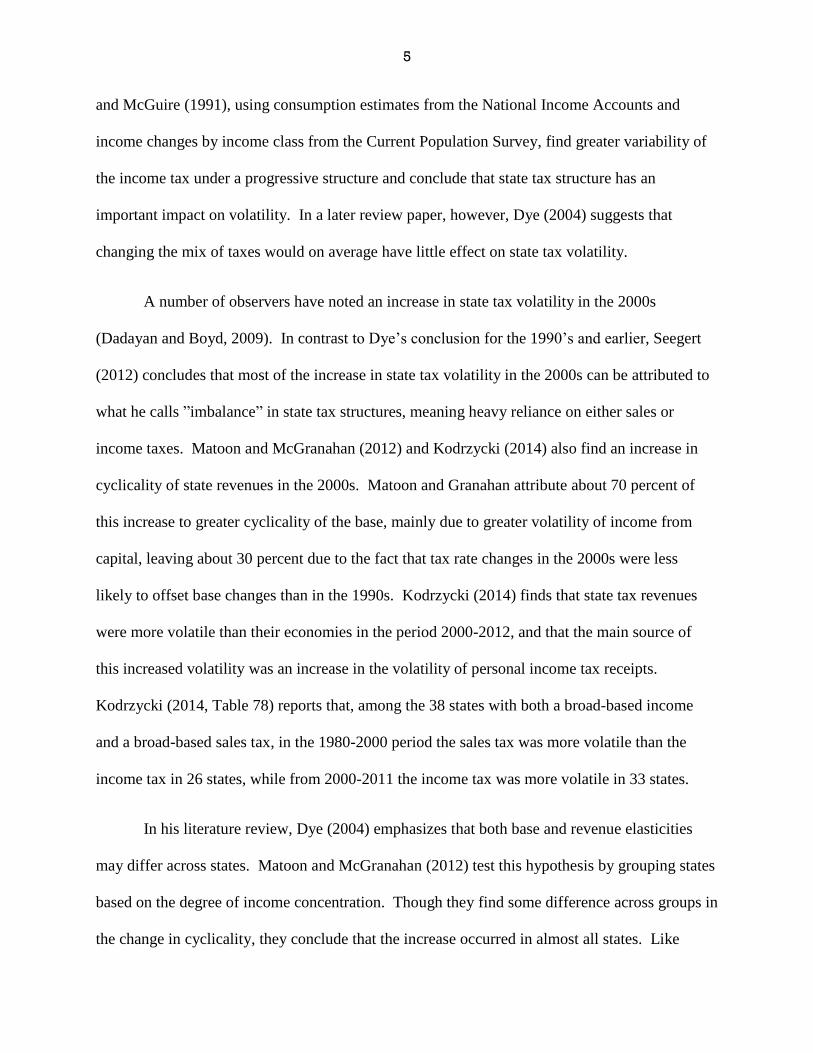
aggregate decline, there was considerable variation across states. As shown in Figure 1, of the
48 contiguous states, 36 had nominal declines in state tax revenue between 2007 and 2009, while
twelve had increases. Part of this variation was due to differences in the impact of the recession,
while part may also have been due to differences across states in tax structure.
While its scope was national, the Great Recession comprised a set of shocks with
differential impacts across income classes, states, and regions. The financial shock, reflected in
sharp drops in capital gains, dividends, and interest income, hit high income households the
hardest (Saez, 2012).2 Hence, the impact was likely to be greatest in states with the greatest
concentration of high income households and the greatest reliance on capital gains and other
income from capital. Among these states are New York, California, Florida, Connecticut, and
Wyoming.
The housing shock – a sharp decline in home values, an increase in mortgage
delinquencies and home foreclosures, and the collapse of the home construction sector – was
greatest in states with the greatest prior run-ups in housing prices; i.e., the largest housing
1 In real terms, state tax revenues in 2012 were 5 percent lower than in 2008. In the 2001 recession, nominal tax
revenues declined for only one year. By 2004, three years after the onset of the recession, nominal revenues were
5.7 percent higher than the previous peak in 2001. In the double-dip recession of 1980-1982, state tax revenues
continued to grow in nominal terms throughout the recession and its aftermath. By 1985, five years after the onset
of the first of the double-dip recessions (and three years after the official end of the second), state tax collections
were up 57.4 percent.
2 Between 2007 and 2009 average real family income fell by 17 percent while real income for the top percentile fell
by 36 percent (Saez, 2012). Aggregate capital gains realizations plummeted from $913 billion in 2007 to $48 billion
in 2009 (Lurie and Pierce, 2012). For filing units with adjusted gross income (AGI) of $200,000 or more,
representing a little less than 5 percent of all returns, capital gains fell by 73 percent between 2007 and 2009.
Interest payments fell by 44 percent, and dividends by 40 percent.

3
bubbles. For example, housing prices in the major metropolitan areas of Arizona, California,
Nevada, and Florida fell by 15 percent or more in both 2008 and 2009, compared with a
nationwide average among large cities of about 5 percent per year (Chernick, Langley and
Reschovsky, 2011). This list suggests substantial overlap between the financial shock and the
housing shock, and indeed California and Florida are among those states with the greatest
potential revenue shocks from the Great Recession (Chernick, Reimers, and Tennant, 2014).
Housing market declines affected the entire income distribution, so that losses were less
concentrated at the top than losses due to the financial shock. Construction and other housing-
related employment losses were also more likely to be concentrated among middle-income
earners.
Other industry-specific shocks also varied in their regional impacts. Declines in financial
services had particularly large impacts in New York, New Jersey, and Connecticut. Michigan
and Rhode Island, both of which had suffered from secular decline in manufacturing, were
among the states where the upper middle of the income distribution was hardest hit. In contrast
to these negative shocks, states such as Wyoming and North Dakota benefited from positive
shocks to the energy sector, while agricultural states such as Iowa benefited from price increases
for corn and wheat. Both the positive and negative shocks had differential impacts across the
income distribution.
This paper challenges the conventional wisdom that attributes revenue volatility to a
state’s dependence on income rather than consumption taxes. We show that this simplistic
model explains very little of the variation in the change in tax revenue across states during the
Great Recession. The variation across states in the relative magnitude of the shocks to different
income classes, together with differences across states in relative tax burdens by income,

4
suggests the desirability of an income distribution-based analysis of revenue volatility. We
introduce a more complex model that takes account of the amounts of income in different slices
of the income distribution and the shocks thereto, as they interact with the tax burden on each
slice. Our approach differs from the conventional analysis of revenue volatility in that we
estimate separate effects, not for each tax, but for changes in income at different points in the
income distribution, interacted with the relevant tax burdens. We find that differences across
states in their income distributions, the distribution of income shocks, and the income-class
incidence of their tax sources are important in explaining the different revenue impacts of the
Great Recession. The distribution of income shocks in turn depends on the state’s industrial
structure, the degree of concentration of income at the top, and the importance of capital gains in
top incomes; whereas the relative burdens depend on the state’s reliance on income vs.
consumption taxes.
The paper has five sections. The first section provides a short literature review. Section
II discusses the models of tax burden and tax revenue change. Section III presents the model
estimates, while Section IV discusses the simulation results. Conclusions are presented in
Section V.
I. Literature Review
Prior research on state tax volatility has used panel data to estimate separate revenue
elasticities for the major state taxes and attempted to distinguish between short and long run
elasticities. Holcombe and Sobel (1997) find similar short run elasticities with respect to
personal income for the sales tax (1.3) and the income tax (1.4) in the period 1972-1993. Dye
5
and McGuire (1991), using consumption estimates from the National Income Accounts and
income changes by income class from the Current Population Survey, find greater variability of
the income tax under a progressive structure and conclude that state tax structure has an
important impact on volatility. In a later review paper, however, Dye (2004) suggests that
changing the mix of taxes would on average have little effect on state tax volatility.
A number of observers have noted an increase in state tax volatility in the 2000s
(Dadayan and Boyd, 2009). In contrast to Dye’s conclusion for the 1990’s and earlier, Seegert
(2012) concludes that most of the increase in state tax volatility in the 2000s can be attributed to
what he calls ”imbalance” in state tax structures, meaning heavy reliance on either sales or
income taxes. Matoon and McGranahan (2012) and Kodrzycki (2014) also find an increase in
cyclicality of state revenues in the 2000s. Matoon and Granahan attribute about 70 percent of
this increase to greater cyclicality of the base, mainly due to greater volatility of income from
capital, leaving about 30 percent due to the fact that tax rate changes in the 2000s were less
likely to offset base changes than in the 1990s. Kodrzycki (2014) finds that state tax revenues
were more volatile than their economies in the period 2000-2012, and that the main source of
this increased volatility was an increase in the volatility of personal income tax receipts.
Kodrzycki (2014, Table 78) reports that, among the 38 states with both a broad-based income
and a broad-based sales tax, in the 1980-2000 period the sales tax was more volatile than the
income tax in 26 states, while from 2000-2011 the income tax was more volatile in 33 states.
In his literature review, Dye (2004) emphasizes that both base and revenue elasticities
may differ across states. Matoon and McGranahan (2012) test this hypothesis by grouping states
based on the degree of income concentration. Though they find some difference across groups in
the change in cyclicality, they conclude that the increase occurred in almost all states. Like

6
Matoon and Granahan, Kodrzycki (2014) finds that the principal source of increased income tax
volatility was an increase in the volatility of the federal tax base.
Though several of these papers note the role of increased volatility of investment
income in the 2000’s, none of them make the link between increased volatility by income source
and increased concentration of income. By contrast, our examination of revenue volatility
during the Great Recession focuses explicitly on the role of differences in the distribution of
income across states and the interaction of those differences with differences in tax structure.
II. Models and Data Sources
To take account of the differential impact of the recession on high income households,
we decompose the shock to each state by income level, using data from the Internal Revenue
Service to obtain changes in adjusted gross income (AGI) by income slice by state. Our analytic
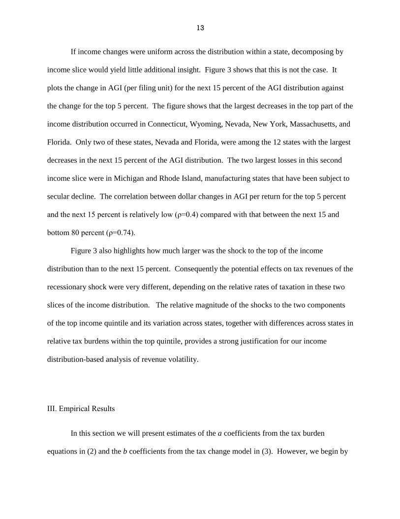
strategy is illustrated in Figure 2. We start with the share of state tax revenue that comes from
the personal income tax and from taxes on consumption. These tax shares are translated into tax
burdens by income slice after dividing the income distribution, as measured by AGI, into three
slices. Tax burdens and base changes for each slice are then used to predict changes in tax
revenue. As shown in the figure, the change in AGI for the top 5 percent depends on the
concentration of income in that group and the importance of capital gains in their income.
Based on available IRS data and our focus on the effect of income changes at the upper
end of the income distribution, families are divided into three income slices: the top 5 percent of
tax filers, the next 15 percent, and the bottom 80 percent. Changes in the tax base by income
level within a state are measured by the change in AGI for that income slice. The data source for

7
AGI by state and AGI bracket is the published Internal Revenue Service Statistics of Income
data (Internal Revenue Service, no date).
Effective tax burdens by income quintile are produced by the Institute for Taxation and
Economic Policy (ITEP, 2009). The Institute for Taxation and Economic Policy is an affiliate of
the better-known Citizens for Tax Justice, and henceforth we will refer to the incidence data as
the “CTJ data.” The CTJ 50-state tax incidence model assigns taxes to families based on
patterns of income and consumption. CTJ measures tax burdens by simulating taxes paid based
on the structure of state income taxes, the rates and coverage of general and specific sales taxes,
and rates of the corporation income tax. Income taxes are assumed to be borne by taxpayers,
while consumption taxes are mainly shifted forward to consumers. In estimating tax burdens, the
CTJ model excludes the portion of taxes that is exported to other states, but does not take
account of taxes imported from other states.3 Estimated tax burdens for the high end of the
state’s income distribution are largely a function of the structure of the personal income tax,
including the top marginal rate, bracket widths, and the tax treatment of capital gains.
Consumption tax burdens are assigned according to spending patterns by income class for taxed
items, using the Consumer Expenditure Survey.
In addition to the tax burden estimates, the CTJ data also provide estimates of average
family income by income slice by state for 2007. The income base used by CTJ for the calculation
of average tax burdens is average family income for a family of four by income slice. Family
income is measured by federal adjusted gross income, plus other items available from the tax
3 While for most states this exclusion makes little difference, for those few states with high revenues from mineral
taxation (severance taxes) or high levels of tourism, the disparity between average tax burdens as measured by the
CTJ and tax collections as a fraction of state personal income could be substantial.

8
returns, such as excluded capital gains and rental and partnership losses.4 The slices are the first
four quintiles, the next fifteen percent, the next four percent, and the top one percent. In contrast, the
published IRS data provide AGI, realized capital gains income, and number of returns by AGI bracket,
state, and year. The brackets are (in thousands): less than $50, $50-$75, $75-$100, $100-200, $200 and
above. To combine the IRS data on changes in income with the CTJ data on tax burdens, we need to
express the IRS data in terms of percentiles. Given the share of returns in each AGI bracket, we use
linear interpolation to assign a share of the AGI and capital gains amounts within each bracket to the
respective percentiles.5 We could not estimate AGI or capital gains amounts for the top one percent,
because the open-ended top AGI bracket ($200,000 or more) contains more than one percent of the
returns in every state. A disproportionate share of the income and capital gains in this bracket belong to
the top one percent, but we have no way of estimating that share, on a state-by-state basis. We therefore
collapse the CTJ data into three slices: the top 5 percent, the next 15 percent, and the bottom 80 percent.6
A. Tax Burdens and Tax Shares
States vary substantially not only in their overall tax burdens but also in their reliance on
different types of taxes and in the resultant distribution of tax burdens by income level. In 2007
on average, 32.2 percent of state tax revenue came from the personal income tax, while 46.7
4 Because the tax return data do not include non–filers, and because most transfer income is excluded from AGI, the
CTJ income measure is not a representative sample of the low-income population.
5 Linear interpolation implicitly assumes that the AGI and capital gains amounts are uniformly distributed within an
AGI bracket. However, national data on the shape of the AGI and capital gains distributions indicates that capital
gains are more concentrated than AGI at the upper end of each bracket. Therefore, linear interpolation understates
the capital-gains share of AGI in the top 5 percent of returns. Unfortunately, the published IRS data are in broad
income brackets, which do not permit a more refined interpolation.
6 In 2007 and 2009 fewer than 5 percent of returns were in the top AGI bracket ($200,000 or above) in every state
but one (New Jersey with 5.1 percent in 2007, and Connecticut with 5.1 percent in 2009). We treat the top AGI
bracket as equivalent to the top 5 percent in New Jersey in 2007 and Connecticut in 2009.

9
percent came from general and selective sales taxes. Table 1 shows the shares in total state tax
revenue of the personal income tax, taxes on consumption, and severance taxes, for the year
2007.
Of the 48 contiguous states, six (South Dakota, Nevada, Washington, Wyoming, Texas,
and Florida) have no income tax, while two (Tennessee and New Hampshire) have very limited
income taxation.7 Of the 40 states that use a broad-based income tax, the rate structure varies
widely. Nineteen tax most income at a single rate. For the rest of the income-tax states, there is
considerable variation in both the top rate and the degree of graduation (Dye, 2004). At the
beginning of the recession in 2007, the highest top marginal rate was in California, at 10.3
percent for taxable income above $1 million (Tax Foundation, 2014).
Differences in the structure of the income tax translate into substantial variation in the
progressivity of the income tax across states. The CTJ estimates indicate that the ratio of the
income tax burdens on the top 5 percent to the bottom 80 percent in a state ranges from 0.94 to
5.8, with an average of 1.84 and standard deviation of 0.95. While nominal rates for the general
sales and excise taxes are typically uniform within states (with some minor variation across
counties), effective consumption tax rates vary by income level because of differences in the
share of taxable consumption in income. Based on data from the Current Expenditure Survey,
the elasticity of consumption of taxable items with respect to annual income is substantially
below one (Poterba, 1989).8 For taxes on consumption, CTJ estimates an average ratio of
7 Tennessee levies a 6 percent tax on dividends, interest, and some capital gains income, while New Hampshire has
a 5 percent rate on interest and dividend income.
8 There has been some debate concerning the long run income class incidence of consumption taxes. A number of
economists argue that the ratio of taxable consumption to income varies much less when one measures income over
a time period longer than a year. For example, Poterba (1989) finds that the gasoline tax is substantially less
regressive when one uses annual consumption as a proxy for permanent or longer run income than when one uses
annual income. In constrast, Chernick and Reschovsky (1997), using 11 years of panel data on individual families,

10
effective tax burdens on the top to middle quintile equal to 0.53. Variation around this average
across states is small (standard deviation = .03), suggesting that variation across states in the
taxable base has relatively little effect on the incidence of consumption taxes, at least in the
upper part of the income distribution.
In this paper we model the level and distribution of state tax burdens as a function of the
relative reliance on the two major types of state taxes: personal income and consumption taxes
(both general sales and excise taxes). The share of total tax revenue from each of these taxes is
equal to the weighted average of the burdens of that tax by income slice (where the weights are
the share of each slice in the tax base for that tax), multiplied by the total tax base and divided by
total state tax revenue. For both income and consumption taxes, the tax base is measured by
AGI. Tax shares are equal to
𝑆𝐻𝑅𝑝𝑖𝑡,𝑐𝑜𝑛𝑠 = 𝐵𝑢𝑟𝑑𝑝𝑖𝑡,𝑐𝑜𝑛𝑠
𝐴𝐺𝐼
𝑇𝑜𝑡𝑡𝑎𝑥
= [(∑ 𝐵𝑢𝑟𝑑3
𝑖=1 {𝑝𝑖𝑡,𝑐𝑜𝑛𝑠},𝑖 𝑆ℎ𝑟𝐴𝐺𝐼𝑖)] ∙ 𝐴𝐺𝐼
𝑇𝑜𝑡𝑡𝑎𝑥 (1)
In (1), SHR is the share of total state tax revenue (Tottax) from each type of tax, pit refers
to the personal income tax, cons are taxes on consumption, including general and selective sales
taxes, Burd is the effective tax rate, ShrAGI is the share of total AGI, and i indexes slices of the
income distribution. Our estimation procedure essentially inverts equation (1), by regressing
burdens by income class on tax shares. With states indexed by s, we estimate equations of the
form
find that the gasoline tax is only slightly less regressive over the intermediate term than when one uses annual
income.

11
𝐵𝑢𝑟𝑑𝑖𝑠 =
𝑎0𝑖 + 𝑎1𝑖 𝑆𝐻𝑅𝑝𝑖𝑡,𝑠 + 𝑎2𝑖𝑆𝐻𝑅𝑐𝑜𝑛𝑠,𝑠 + 𝑎3𝑖𝑆𝐻𝑅𝑠𝑒𝑣,𝑠 + 𝑎4𝑖 (𝑇𝑜𝑡𝑡𝑎𝑥
𝐼𝑛𝑐𝑜𝑚𝑒)
𝑠+ 𝑒𝑟𝑟𝑜𝑟𝑖𝑠 (2)
The dependent variable 𝐵𝑢𝑟𝑑𝑖 is the effective tax burden on the 𝑖𝑡ℎ income slice. 𝑆𝐻𝑅𝑠𝑒𝑣 is the
share from severance taxes, and Tottax/Income is total state taxes relative to personal income.9
While in most states taxes on consumption and personal income contribute the preponderance of
state tax revenue, a few states are heavily dependent on severance taxes. Because tax shares are
correlated by construction, omitting severance taxes would bias the estimates of the income and
consumption tax effects. The total tax burden is included as a measure of the size of the state’s
public sector, with the expectation that a larger public sector is associated with higher tax
burdens on all income slices.
The coefficients in (2) represent the average relationship between the revenue share from
each tax and the burden on a particular income slice, holding constant the shares of other taxes.
For example, the coefficients of income tax share summarize the effects on the burden for each
income slice, for the state with the average degree of income tax progressivity and the average
income distribution. The equation may underestimate the burden on the top 5 percent in states
whose income tax is substantially more graduated than the average. By contrast, it may
overestimate the burden on the top 5 percent for states such as Connecticut, that have an average
degree of income tax progressivity but a very high proportion of total AGI in the top income
slice.
9 The major tax omitted from (2) is the corporation income tax (CIT), which in aggregate provided less than seven
percent of state tax revenues. A portion of each state’s CIT is borne by the owners of capital in other states and is
not captured in the CTJ methodology.

12
B. Tax Revenue Change Model
The model of tax revenue change is written as
𝑇𝐴𝑋𝑠 = 𝑏0 + ∑ 𝑏1𝑖31 𝐵𝑢𝑟𝑑𝑖𝑠 + ∑ 𝑏2𝑖
31 ∆𝐴𝐺𝐼𝑖𝑠 + ∑ 𝑏3𝑖
31 𝐵𝑢𝑟𝑑𝑖𝑠 ∗ ∆𝐴𝐺𝐼𝑖𝑠 + 𝑒𝑟𝑟𝑜𝑟𝑖𝑠 (3)
where TAX is the change in state tax revenue from 2007 to 2009, scaled by the number of
federal income tax returns in 2007. Tax rates t are the effective burdens on the three slices i of
the AGI distribution, the ∆𝐴𝐺𝐼′𝑠 are the changes in federal adjusted gross income between 2007
and 2009 for the three slices, each scaled by the number of 2007 federal tax returns from that
slice. The third set of terms are the interactions between the tax rate and the change in the tax
base.
If tax policy responses were systematically related to the magnitude of the base decline,
either in total or in particular slices of the income distribution, then the estimates of (3) would be
biased, thus undermining the validity of the estimate-based simulations which follow.10
In
Chernick, Reimers and Tennant (2014) we calculated the difference between actual tax changes
and potential revenue exposure, where the latter equals the weighted average of the initial tax
burden times the change in AGI per return for each income slice. We found that none of the
regressors in (3) was correlated with this difference at the 5 percent significance level.11
This
suggests that the potential bias from correlation of the error term with the regressors in (3) is
unlikely to be very severe.
10 Poterba (1994) found just such an offset in the 1988–1992 period, with state tax responses to unexpected negative
deficit shocks proportional to the magnitude of the shock. However, as noted above, Matoon and McGranahan
(2012) find that tax rate changes in the 2000s were less likely to offset base changes than in the 1990s.
11 At the ten percent level of significance, changes in top 5 percent AGI were negatively correlated (Pearson
correlation coefficient) with the difference, while changes in the next 15 percent were positively correlated with it.
13
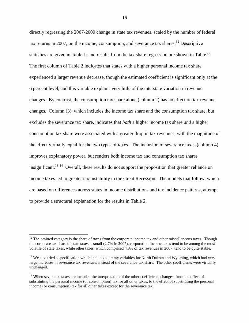
If income changes were uniform across the distribution within a state, decomposing by
income slice would yield little additional insight. Figure 3 shows that this is not the case. It
plots the change in AGI (per filing unit) for the next 15 percent of the AGI distribution against
the change for the top 5 percent. The figure shows that the largest decreases in the top part of the
income distribution occurred in Connecticut, Wyoming, Nevada, New York, Massachusetts, and
Florida. Only two of these states, Nevada and Florida, were among the 12 states with the largest
decreases in the next 15 percent of the AGI distribution. The two largest losses in this second
income slice were in Michigan and Rhode Island, manufacturing states that have been subject to
secular decline. The correlation between dollar changes in AGI per return for the top 5 percent
and the next 15 percent is relatively low (ρ=0.4) compared with that between the next 15 and
bottom 80 percent (ρ=0.74).
Figure 3 also highlights how much larger was the shock to the top of the income
distribution than to the next 15 percent. Consequently the potential effects on tax revenues of the
recessionary shock were very different, depending on the relative rates of taxation in these two
slices of the income distribution. The relative magnitude of the shocks to the two components
of the top income quintile and its variation across states, together with differences across states in
relative tax burdens within the top quintile, provides a strong justification for our income
distribution-based analysis of revenue volatility.
III. Empirical Results
In this section we will present estimates of the a coefficients from the tax burden
equations in (2) and the b coefficients from the tax change model in (3). However, we begin by
14
directly regressing the 2007-2009 change in state tax revenues, scaled by the number of federal
tax returns in 2007, on the income, consumption, and severance tax shares.12
Descriptive
statistics are given in Table 1, and results from the tax share regression are shown in Table 2.
The first column of Table 2 indicates that states with a higher personal income tax share
experienced a larger revenue decrease, though the estimated coefficient is significant only at the
6 percent level, and this variable explains very little of the interstate variation in revenue
changes. By contrast, the consumption tax share alone (column 2) has no effect on tax revenue
changes. Column (3), which includes the income tax share and the consumption tax share, but
excludes the severance tax share, indicates that both a higher income tax share and a higher
consumption tax share were associated with a greater drop in tax revenues, with the magnitude of
the effect virtually equal for the two types of taxes. The inclusion of severance taxes (column 4)
improves explanatory power, but renders both income tax and consumption tax shares
insignificant.13
14
Overall, these results do not support the proposition that greater reliance on
income taxes led to greater tax instability in the Great Recession. The models that follow, which
are based on differences across states in income distributions and tax incidence patterns, attempt
to provide a structural explanation for the results in Table 2.
12 The omitted category is the share of taxes from the corporate income tax and other miscellaneous taxes. Though
the corporate tax share of state taxes is small (2.7% in 2007), corporation income taxes tend to be among the most
volatile of state taxes, while other taxes, which comprised 4.3% of tax revenues in 2007, tend to be quite stable. 13
We also tried a specification which included dummy variables for North Dakota and Wyoming, which had very
large increases in severance tax revenues, instead of the severance-tax share. The other coefficients were virtually
unchanged.
14 When severance taxes are included the interpretation of the other coefficients changes, from the effect of
substituting the personal income (or consumption) tax for all other taxes, to the effect of substituting the personal
income (or consumption) tax for all other taxes except for the severance tax.

15
A. Tax Burdens
As shown in Figure 2 and equation (2), tax burdens are assumed to depend on the shares
of income, consumption, and severance taxes in total tax revenue, as well as the overall burden
of taxation. Estimates of the tax burden models are shown in Table 3. Tax shares are most
successful in explaining the variation in burden for the top quintile, with an adjusted R2 equal to
0.76 for the top 5 percent and 0.65 for the next 15 percent, but only 0.43 for the bottom 80
percent. The coefficient estimates show the effect on burdens of substituting each of the listed
taxes for the omitted category, which is “other” taxes, including the corporation income tax and
license taxes. Notably, the income tax share has a significantly positive effect on all burdens
across the income distribution, with the effects on the top-5 and next-15 burdens almost equal,
and only slightly larger than the effect on the next-80 burden. Thus, the main effect of a higher
personal income tax share is to increase state tax burdens across the board, with relatively small
differences across the income distribution.
Greater reliance on consumption taxes has a regressive impact, with an insignificant
effect on the top-5 burden, but increasing the bottom-80 burden 70 percent more than the next-15
burden. The contrast between the incidence effects of the income and consumption tax shares is
striking. Compared with the consumption-tax share, the personal income-tax share has four
times the effect on the top-5 burden, twice the effect on the next-15 burden, and about the same
effect on the bottom-80 burden.
As shown in row 3 of Table 3, a higher severance tax share is associated with lower
burdens on the top quintile of the AGI distribution, but has no significant effect on the burden on
the bottom 80 percent. Severance tax revenues are determined by mineral prices in world

16
markets and by the available supply, given the state of technology. The results in Table 3 suggest
that states use these revenues to reduce tax burdens on the top quintile of the income distribution.
The overall tax burden is a measure of preferences for public services.15
A higher overall tax
burden is associated with higher tax burdens across the income distribution (Table 3, row 4).
However, the effect of the overall burden is greater the higher the income slice, suggesting that a
more progressive tax structure accompanies, or is required for, a larger public sector.
We can use the results in Table 3 to answer the following question: What would be the
effect on tax burdens across the distribution of a marginal substitution of the income tax for taxes
on consumption, holding constant their combined share of total tax revenue? The net effect on
burdens of such a change, taking account of both the offsetting change in the consumption tax
share and of their combined share in total tax revenue, is shown in Table 4. This net effect is
smaller than the coefficient of the income tax share shown in Table 3, where a higher income tax
share or consumption tax share comes at the expense of lower shares of the omitted taxes. In
Table 4 an increase in the income tax share implies a lower consumption tax share, while the
share of omitted taxes is constant. Since we know from Table 3 that the consumption tax share
has a positive effect on tax burdens when it is substituted for the omitted taxes, the net effect of
increasing the income tax share is smaller when we reduce the consumption tax share instead of
the share of omitted taxes.
Whereas Table 3 showed that substituting the income tax for “other” taxes (keeping the
consumption tax share constant) raises burdens more or less equally across all income slices,
Table 4 shows that substituting the income tax for consumption taxes has a progressively smaller
15
This statement is subject to the caveat that higher states taxes may be at least partially offset by lower local taxes.

17
effect as we move down the income distribution. Evaluated at the mean share of income and
consumption taxes in total state taxes (0.79), a ten percentage point increase in the income tax
share of combined income and consumption taxes (e.g., from 40 percent to 50 percent) would
raise tax burdens on the top 5 percent by half a percentage point, and on the next 15 percent by a
third of a percentage point. There is no effect on the bottom 80 percent. Not surprisingly, the
expressions in Table 4 show that the effects of changing income and consumption tax shares will
be larger, the more states rely on these two types of taxes.
B. Change in Tax Revenues
Estimates of the model of change in total tax revenue per return (equation 3) are shown in
Table 5. When interpreting the results from Table 5, it should be kept in mind that these are
cross-state, not longitudinal within-state effects. The adjusted R2 is 0.58, indicating that our
distributional model captures factors that are important in explaining the variation in state tax
revenue changes.16
The model is discussed more fully in Chernick, Reimers, and Tennant
(2014). Here we emphasize the marginal impact of the tax burdens for each of the three income
slices. 17
Manipulating the estimated coefficients in Table 5, the marginal impact on the 2007-
2009 tax revenue change is equal to
𝜕(∆𝑇𝑎𝑥𝑠) = (16277 + . 296 ∗ ∆𝐴𝐺𝐼𝑡𝑜𝑝5,𝑠) ∗ 𝜕(𝐵𝑢𝑟𝑑𝑡𝑜𝑝5,𝑠 ) + (−9935 − 6.116 ∗
∆𝐴𝐺𝐼𝑛𝑥𝑡15,𝑠 ) ∗ 𝜕(𝐵𝑢𝑟𝑑𝑛𝑥𝑡15,𝑠) + (−16339 − 3.114 ∗ ∆𝐴𝐺𝐼𝑛𝑥𝑡80,𝑠) ∗ 𝜕(𝐵𝑢𝑟𝑑𝑛𝑥𝑡80,𝑠) (4)
16 In an alternative specification that includes dummy variables for North Dakota and Wyoming (outliers with huge
increases in revenue from severance taxes -- see Figure 1), the adjusted R2 increases to .87.
17 Because the dollar change in taxes and the percentage change are almost perfectly correlated (rho = .97), the
results, though estimated less precisely, are basically unaffected if we replace the dollar amount of tax change with
the percentage change. In terms of policy interpretation, we would argue that the dollar change is more relevant.

18
In (4), TAX is the 2007-2009 dollar change in tax revenue, AGI is the change in
adjusted gross income for the respective income slice (top 5, next 15 and bottom 80 percent), and
Burd is the tax burden for the income slice. To make states comparable, TAX and AGI are
divided by the number of federal income tax returns in the income slice in 2007. We expected
that, holding the change in AGI constant, a higher tax burden at any point in the income
distribution would be associated with a greater change in tax revenues. Similarly, the greater the
change in the tax base (i.e., AGI) at any income level, the greater the expected revenue response.
Table 5 shows that the burden and base-change effects are non-linear, depending on the
interaction between the two, and that the direction of effect differs across the income
distribution. For states where top-5 AGI fell by $55,000 or more, the higher the tax burden, the
greater the decrease in total tax revenues. At the mean change in adjusted gross income for the
top 5 percent (‒$84,000), a one percentage-point increase in the tax burden would increase the
revenue loss by $86 per return, nearly two thirds again as much as the average reduction of
$138. Despite the fact that, unlike the rest of the distribution, the average change in AGI was
positive for the bottom 80 percent, the effect of higher tax burdens on this slice, like the effect for
the top 5 percent, is to exacerbate the decline in total tax revenues. At the mean change in
bottom-80 AGI of +$1100, a one percentage-point increase in the tax burden is associated with a
$198 (per return) larger reduction in total tax revenues.
In contrast, states with higher tax burdens on the next 15 percent, all else equal,
experienced a smaller hit to tax revenues. The second term in equation (4) implies that for states
with reductions in next-15 AGI of $1625 per return or more (which was the case for all but three
states), the net effect of a higher next-15 burden is positive; that is, to reduce the tax loss. At the
mean change in next-15 AGI (-$5260), a one percentage-point increase in the next-15 burden

19
corresponds to a $222 (per return) smaller loss (or larger gain) of tax revenues. These results
reflect the pattern across states of total tax revenue changes combined with AGI changes and tax
burdens by income slice. It is possible that unobserved factors that are correlated with the
burden on the next 15 percent produce more tax revenue in states with a higher burden on that
income group.18
In any case, the result suggests that differences across states in tax burdens by
income level may have unpredictable effects on revenue volatility. The difference in burden
effects across income slices will turn out to be crucial for explaining the simulation results in the
next section.
IV. Using Predicted Tax Burdens to Simulate Revenue Changes
The goal in this section is to use the estimated coefficients from the tax burden and tax
change regressions (Tables 3 and 5) to predict how the recession-induced change in tax revenues
would have been affected under the counterfactual assumption of a more balanced (i.e., national
average) mix of income and consumption taxes in each state. The analysis proceeds in two
stages. First we use the predicted tax burdens from the tax share regressions in Table 3, given
actual 2007 tax shares, together with the coefficient estimates from Table 5, to generate baseline
simulations of the 2007-2009 change in tax revenue. We then simulate the burdens when we
replace actual income- and consumption-tax shares (of their combined total) with the 2007
averages for all states. We use these simulated burdens with the coefficients from the tax change
regression to simulate the state-by-state change in tax revenue under the hypothetical balanced
18 One possible explanation for the counterintuitive effect of next-15 tax burdens is that estimates of tax changes are
confounded by the cyclical behavior of state corporation income taxes. Though small as a share of total state tax
revenues, the corporation income tax is extremely volatile. However, when we excluded the corporation income tax
from our measure of the change in taxes, the results were unaffected.
20
system. While a nationally uniform, more balanced system of income and consumption taxes is
of course unrealistic, and actual adjustments in tax shares are likely to be incremental, we believe
there is considerable insight to be gained from an examination of this extreme case.
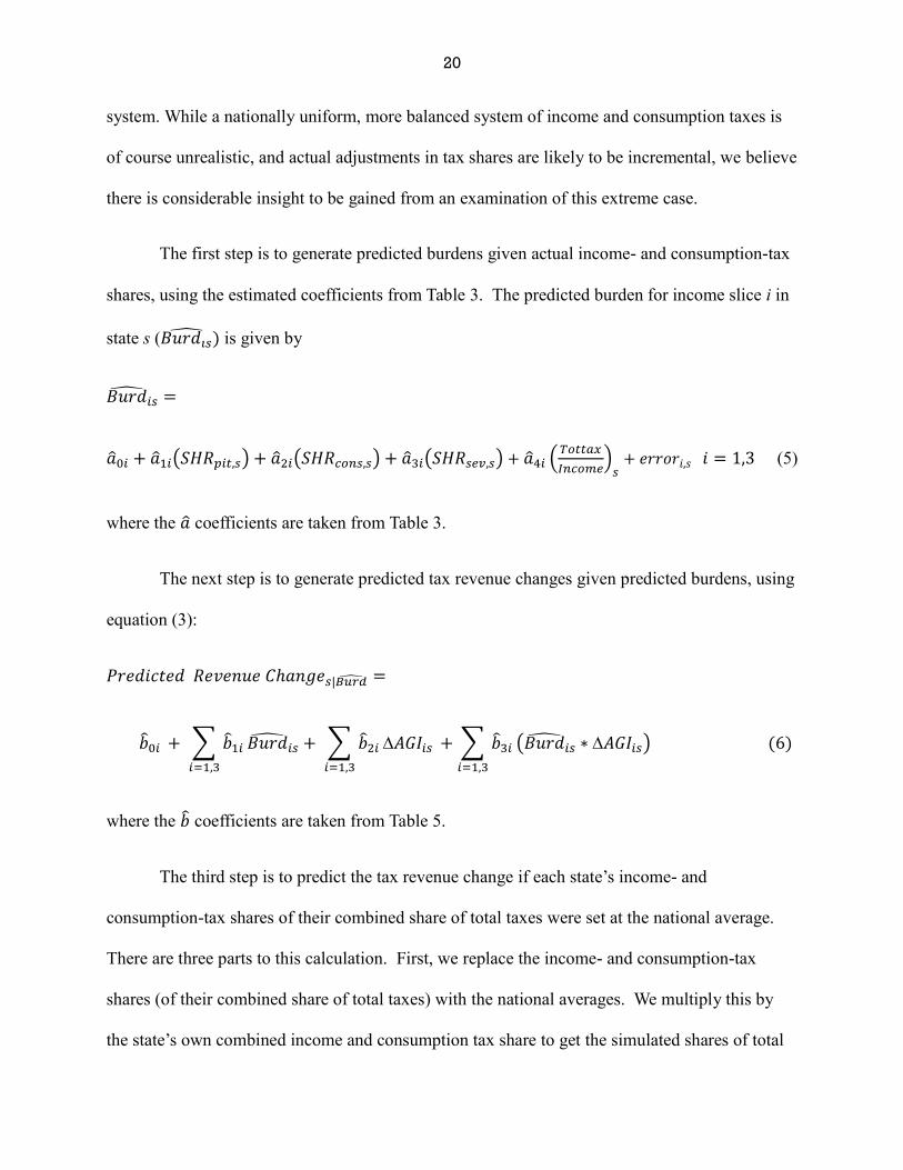
The first step is to generate predicted burdens given actual income- and consumption-tax
shares, using the estimated coefficients from Table 3. The predicted burden for income slice i in
state s (𝐵𝑢𝑟𝑑𝑖𝑠̂ ) is given by
𝐵𝑢𝑟�̂�𝑖𝑠 =
�̂�0𝑖 + �̂�1𝑖(𝑆𝐻𝑅𝑝𝑖𝑡,𝑠) + �̂�2𝑖(𝑆𝐻𝑅𝑐𝑜𝑛𝑠,𝑠) + �̂�3𝑖(𝑆𝐻𝑅𝑠𝑒𝑣,𝑠) + �̂�4𝑖 (𝑇𝑜𝑡𝑡𝑎𝑥
𝐼𝑛𝑐𝑜𝑚𝑒)
𝑠+ 𝑒𝑟𝑟𝑜𝑟𝑖,𝑠 𝑖 = 1,3 (5)
where the �̂� coefficients are taken from Table 3.
The next step is to generate predicted tax revenue changes given predicted burdens, using
equation (3):
𝑃𝑟𝑒𝑑𝑖𝑐𝑡𝑒𝑑 𝑅𝑒𝑣𝑒𝑛𝑢𝑒 𝐶ℎ𝑎𝑛𝑔𝑒𝑠|𝐵𝑢𝑟�̂� =
�̂�0𝑖 + ∑ �̂�1𝑖
𝑖=1,3
𝐵𝑢𝑟�̂�𝑖𝑠 + ∑ �̂�2𝑖
𝑖=1,3
𝐴𝐺𝐼𝑖𝑠 + ∑ �̂�3𝑖
𝑖=1,3
(𝐵𝑢𝑟�̂�𝑖𝑠 ∗ 𝐴𝐺𝐼𝑖𝑠) (6)
where the �̂� coefficients are taken from Table 5.
The third step is to predict the tax revenue change if each state’s income- and
consumption-tax shares of their combined share of total taxes were set at the national average.
There are three parts to this calculation. First, we replace the income- and consumption-tax
shares (of their combined share of total taxes) with the national averages. We multiply this by
the state’s own combined income and consumption tax share to get the simulated shares of total

21
taxes. Next, we calculate the predicted burdens using the �̂�s from Table 3 and these simulated
tax shares, while keeping the state’s own severance tax share and overall tax burden unchanged:
𝐵𝑢𝑟�̂�(𝑖𝑠| 𝑆𝐻𝑅𝑠) =
�̂�0𝑖 + �̂�1𝑖(𝑆𝐻𝑅̅̅ ̅̅ ̅̅𝑝𝑖𝑡/(𝑐𝑜𝑛𝑠+𝑝𝑖𝑡)) ∗ 𝑆𝐻𝑅(𝑐𝑜𝑛𝑠+𝑝𝑖𝑡)𝑠 + �̂�2𝑖(𝑆𝐻𝑅̅̅ ̅̅ ̅̅
𝑐𝑜𝑛𝑠/(𝑐𝑜𝑛𝑠+𝑝𝑖𝑡)) ∗ 𝑆𝐻𝑅(𝑐𝑜𝑛𝑠+𝑝𝑖𝑡)𝑠 +
�̂�3𝑖(𝑆𝐻𝑅)𝑠𝑒𝑣,𝑠 + �̂�4𝑖 (𝑇𝑜𝑡𝑡𝑎𝑥
𝐼𝑛𝑐𝑜𝑚𝑒)
𝑠+ 𝑒𝑟𝑟𝑜𝑟𝑖,𝑠 𝑖 = 1,3 (7)
We then calculate the predicted change in tax revenue using the predicted burdens from equation
(7). The prediction equation is given by
𝑃𝑟𝑒𝑑𝑖𝑐𝑡𝑒𝑑 𝑅𝑒𝑣𝑒𝑛𝑢𝑒 𝐶ℎ𝑎𝑛𝑔𝑒𝑠,(𝐵𝑢𝑟�̂�|𝑆𝐻𝑅̅̅ ̅̅ ̅̅ 𝑠) =
�̂�0𝑖 + ∑ �̂�1𝑖𝑖=1,3 𝐵𝑢𝑟�̂�𝑖,𝑠|𝑆𝐻𝑅𝑠 + ∑ �̂�2𝑖𝑖=1,3 𝐴𝐺𝐼𝑖,𝑠 + ∑ �̂�3𝑖𝑖=1,3 (𝐵𝑢𝑟�̂�𝑖,𝑠|𝑆𝐻𝑅𝑠 ∗ 𝐴𝐺𝐼𝑖,𝑠) (8)
Since the overall burden is a weighted average of the burdens by income slice, it will
change when any of these burdens change:
𝑆𝑖𝑚𝑢𝑙𝑎𝑡𝑒𝑑 𝑂𝑣𝑒𝑟𝑎𝑙𝑙 𝐵𝑢𝑟𝑑𝑠 = ∑ (𝐴𝐺𝐼𝑖𝑠/𝐴𝐺𝐼𝑠)𝑖=1,3 ∗ 𝐵𝑢𝑟�̂� (𝑖.𝑠|𝑆𝐻𝑅𝑠) (9)
The final exercise is to simulate the effect on tax changes under uniform personal income
tax and consumption tax shares, while maintaining the initial tax burden. The objective here is to
separate the tax incidence effect from the overall burden effect. To do this, we preserve the
simulated relative burdens across income slices, while adjusting the burden on each slice
proportionally:

22
𝐵𝑢𝑟�̂�𝑖,𝑠|(𝑆𝐻𝑅𝑠,𝑜𝑣𝑒𝑟𝑎𝑙𝑙 𝑏𝑢𝑟𝑑 𝑐𝑜𝑛𝑠𝑡𝑎𝑛𝑡) = [𝐵𝑢𝑟�̂�𝑖𝑠|𝑆𝐻𝑅𝑠)] ∗ (𝐴𝑐𝑡𝑢𝑎𝑙 𝑜𝑣𝑒𝑟𝑎𝑙𝑙 𝑏𝑢𝑟𝑑
𝑆𝑖𝑚𝑢𝑙𝑎𝑡𝑒𝑑 𝑜𝑣𝑒𝑟𝑎𝑙𝑙 𝑏𝑢𝑟𝑑)
𝑠 (10)
Finally, we calculate the predicted revenue change, using the predicted burdens from (10) and the
estimates of �̂� from Table 5:
𝑃𝑟𝑒𝑑𝑖𝑐𝑡𝑒𝑑 𝑅𝑒𝑣𝑒𝑛𝑢𝑒 𝐶ℎ𝑎𝑛𝑔𝑒𝑠,[(𝐵𝑢𝑟�̂�|(𝑆𝐻𝑅̅̅ ̅̅ ̅̅ 𝑠,𝑜𝑣𝑒𝑟𝑎𝑙𝑙 𝑏𝑢𝑟𝑑 𝑐𝑜𝑛𝑠𝑡𝑎𝑛𝑡)] =
�̂�0𝑖 + ∑ �̂�1𝑖𝑖=1,3 𝐵𝑢𝑟�̂�𝑖,𝑠 |(𝑆𝐻𝑅𝑠,𝑜𝑣𝑒𝑟𝑎𝑙𝑙 𝑏𝑢𝑟𝑑 𝑐𝑜𝑛𝑠𝑡𝑎𝑛𝑡) + ∑ �̂�2𝑖𝑖=1,3 𝐴𝐺𝐼𝑖,𝑠 +
∑ �̂�3𝑖𝑖=1,3 (𝐵𝑢𝑟�̂�(𝑖,𝑠 |(𝑆𝐻𝑅𝑠,𝑜𝑣𝑒𝑟𝑎𝑙𝑙 𝑏𝑢𝑟𝑑 𝑐𝑜𝑛𝑠𝑡𝑎𝑛𝑡) ∗ 𝐴𝐺𝐼𝑖,𝑠) (11)
The tax change simulations from (11), with constant overall burdens, can then be compared to
(8), where overall burdens are allowed to change
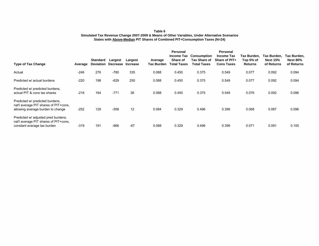
Tables 6 and 7 show the key results from our analysis. States are broken into two groups,
based on the personal income tax share of combined income and consumption taxes. Other taxes,
including severance, corporate, and inheritance taxes, are outside the scope of our analysis,
hence taken as exogenous. In Table 6 we consider states whose income tax share is above the
median. Table 7 includes states whose income tax share is below the median, excluding the two
states with the highest severance tax share of revenue, for the reason discussed below. The
simulation exercise assigns all states the national average income tax share of income plus
consumption taxes. Hence, states in Table 6 would get a smaller share of tax revenues from the
personal income tax, while states in Table 7 would get a larger share. According to the
conventional wisdom, one would expect the states in Table 6 to see a decrease in volatility under

23
the simulation (i.e., a smaller revenue hit), while states in Table 7 would see an increase in
volatility (i.e., a bigger hit).
The first row of Tables 6 and 7 shows the actual tax revenue change for the two groups of
states. It is noteworthy that the average changes, a decrease of $246 per return for the high
income-tax-share states and a decrease of $233 for the low income-tax states, are quite similar in
sign and magnitude. The exclusion of the two highest severance-tax states, Wyoming and North
Dakota, is key to the latter result.19
Both states experienced substantial increases in tax revenue
during the Great Recession, due mainly to large increases in severance tax revenues from
expanded oil, gas, and coal production. As shown in Table 3, states tend to use severance tax
revenues to reduce tax burdens, especially on the high income groups. Hence, in addition to the
severance tax windfall, low tax burdens in Wyoming and North Dakota, plus the fact that AGI
actually increased in North Dakota, tended to mute the effect of the recession on tax revenue.
Nevertheless, whether these two states are included or not, the predicted revenue hit at national
average shares is smaller than at the actual shares.
In Tables 6 and 7, row 3 summarizes predicted revenue changes using actual tax shares to
predict burdens by income class. Predicted tax changes under the simulation models (rows 4 and
5) are compared with row 3. Substituting national averages for actual income-tax shares affects
both the incidence of state tax systems and the overall tax burden. For high income-tax states,
increasing the consumption tax share makes the tax system more regressive while lowering the
overall burden. For low income-tax states, the opposite occurs when the national averages are
19 Including these states would reduce the average actual revenue cut for the below-median income tax states to ‒
$29 from ‒$233. In 2007 Wyoming got 40 percent of its tax revenue from severance taxes, and North Dakota got 22
percent. These two states, though small in terms of population and share of aggregate state tax revenues, also have
low income tax shares.

24
substituted – less regressivity and a higher overall burden. Row 4 shows both effects combined,
while row 5 takes account of the incidence effect alone, while keeping overall burdens constant.
Row 4 of Table 6 shows that increasing the regressivity of high income-tax-share systems by
increasing the consumption tax share, and allowing the state tax burden to decrease, would have
resulted in a greater average hit to tax revenues than is predicted by the actual mix of taxes, with
the simulated decrease going from ‒$218 to ‒$252. Row 5 shows that a more regressive tax
system by itself would have led to a substantially larger tax hit to these states than if the overall
burden were allowed to drop as well - ‒$319 instead of ‒$252. These results suggest that the
effect on the average tax burden partially offsets the regressivity effect, as a lower average
burden by itself reduces the tax hit, while a more regressive tax structure increases it.
Table 7 shows the opposite effect for the low income-tax states. Making them less
regressive, while allowing their overall tax burden to increase, reduces the average predicted tax
hit from the recession from ‒$228 to ‒$202. Keeping their smaller public sector size (i.e.,
holding the overall tax burden constant), but imposing a more progressive tax system, would
further reduce the average tax hit from ‒$202 all the way down to ‒$161. As in Table 6, the
effect on the overall burden partially offsets the progressivity effect, as a heavier overall tax
burden increases the tax hit, while a less regressive tax structure reduces it.
These results are quite remarkable. They suggest that, contrary to the conventional
wisdom, low income-tax states would have had better revenue performance during the Great
Recession with a more balanced tax structure, while high income-tax states would have had
worse performance had they had a more balanced tax structure. To explain these
counterintuitive results, it is useful to look more specifically at states at the extremes, with the
greatest and least reliance on the personal income tax. Table 8 compares simulated to predicted

25
revenue changes for the 5 states with the highest shares of the personal income tax in the
combined total of income plus consumption taxes, while Table 9 looks at the 5 states with no
personal income tax, other than Wyoming.20
In these states, the simulation exercise of setting
income and consumption tax shares to their national averages represents especially large changes
in tax structure.
The results in Table 8, for the states with the five highest income-tax shares, are
remarkably similar to those in Table 6. A lower income tax share would have resulted in a larger
revenue hit from the recession. The fourth row of Table 8 indicates that reducing the income tax
share to its national average would have lowered the income tax share from 70 to 40 percent of
income plus consumption taxes. After adjusting to keep the overall burden constant, this change
would have reduced the predicted top-5 burden from 8.2 to 6.9 percent, and the predicted next-15
burden from 9.5 to 8.9 percent. The predicted revenue hit would have been 63 percent greater
than the predicted hit under the actual tax shares, ‒$419 instead of ‒$224. Equally high but
much more regressive tax burdens would have increased the fiscal vulnerability of the high
income tax states.
Why would high income tax states have been hit harder on average had they been less
reliant on the income tax? Inspection of the individual states in this group shows that the results
vary by state. In line with conventional wisdom about the greater volatility of income taxes, if
the overall tax burden were held constant while the income-tax share is reduced to the national
average, a reduced revenue hit would be predicted for Massachusetts. However, this reduction is
20
The five states with the greatest reliance on the income tax relative to consumption taxes are Oregon, Delaware,
Massachusetts, New York, and Virginia. The six states with no personal income tax are Florida, Nevada, South
Dakota, Texas, Washington, and Wyoming. We exclude Wyoming from Table 9 because it got a huge windfall
increase in revenue from severance taxes, which contribute 40 percent of its tax revenues.

26
outweighed by an increased hit for Delaware, New York, Virginia, and especially Oregon. If the
overall tax burden were allowed to change along with the income-tax share, New York would
join Massachusetts in having a reduced revenue hit. Thus, New York’s result is also consistent
with the conventional wisdom.
However, for Delaware, Oregon, and Virginia the reduction in top quintile tax burdens
would have increased the hit to revenues. The reason is that in these three states the decline in
AGI for the top 5 percent was relatively small, muting the reduction in the revenue hit that
results from the (simulated) reduction in the top-5 tax burden. In Oregon, moreover, the
recession led to a particularly large decline in AGI for the next 15 percent of the income
distribution, fully 65 percent greater than the national average. Recalling from Table 5 that a
higher tax burden on the next 15 percent was associated with a smaller rather than a larger
revenue hit, the large decline in AGI magnified the negative effect of the simulated decrease in
the next-15 burden, leading to an increase in Oregon’s revenue hit. The Oregon result strikingly
illustrates that revenue volatility reflects a complicated interaction between tax structure and the
size and distribution of recession-induced changes in the tax base.21
Table 9 shows the results for states without an income tax, other than Wyoming.
Compared with the high income-tax share states in Table 8, these states have average tax burdens
21
New Jersey is another state with a relatively progressive tax structure, high concentration of income in the top 5
percent, and high overall tax burden. A shift to a smaller income tax share would therefore have lowered volatility.
A rough calculation is that if New Jersey were to substitute neighboring Pennsylvania's flat income tax for its
progressive income tax, but maintain the same overall income tax burden, the hit to New Jersey's income tax
revenue would have been about 40 percent lower. Overall, such a substitution would have reduced the recession-
induced total tax hit by about 30 percent. The cost of this policy is a dramatic increase in regressivity, with the top 5
percent realizing a permanent reduction in effective tax rates of more than two percentage points and the bottom 80
percent seeing a rate increase of two percentage points.

27
that are considerably lower, and much more regressive tax structures.22
Imposing average income
and consumption tax shares in the states without an income tax would have raised the overall tax
burden from 6.1 percent to 7.5 percent. The fifth row of Table 9 shows the predicted revenue
change when we impose the national average income and consumption tax shares, but adjust all
tax burdens proportionally to keep the overall tax burden constant. The predicted revenue
change would rise from ‒$43 to +$24. This result suggests that a more balanced tax structure
would have enabled states with no income tax to better weather the Great Recession.
The last three columns in the first row of Table 9 highlight the extremely regressive tax
structure in these states. Tax burdens on the bottom 80 percent (8.7 percent) were more than 2½
times as high as on the top 5 percent (3.4 percent). Nonetheless, during the Great Recession
these five states mirrored the national trend, realizing an actual revenue decrease of ‒$261.
However, their predicted revenue decrease of ‒$43 using actual tax shares (row 3) is much
smaller than that for the 5 highest income tax states (‒$224, according to Table 8). This would
seem to support the proposition that less reliance on the income tax is likely to reduce fiscal
vulnerability during recessions.
However, the fifth row of Table 9 suggests that in fact, no-income tax states paid a fiscal
penalty for the imbalance in their tax structures. If we alter the tax structure in those states to
make income and consumption tax shares equal to the national average, while keeping the
overall tax burden unchanged, the predicted revenue change would switch from a decrease to an
increase, going from ‒$43 to +$24. In contrast, the fourth row indicates that imposing the
national average tax shares, while also allowing the increase in overall tax burdens that would
22
The average tax burden in the no income tax states is a full 2.3 percentage points lower than in the high income
tax states.

28
result from this change in tax structure, would have increased the predicted reduction in tax
revenues by ‒$31 per return, from ‒$43 to ‒$74, as compared with the prediction based on
actual tax shares (row 3). Comparing rows 4 and 5, the effect of allowing overall burdens to rise
as we substitute income for consumption taxes is to reverse the predicted revenue increase, from
+$24 to ‒$74. Thus for the no-income tax states, a more balanced tax structure, and the higher
overall burdens that typically accompany such a tax structure, would have increased fiscal
vulnerability during the recession.
These results suggest that it is the higher overall burden that tends to go along with state
income taxation, rather than the division of taxes between income and consumption, that
primarily affects revenue resilience. Moreover, recall that Table 8 shows that the lower overall
burden makes revenue less volatile when we reduce the income tax share. Allowing the overall
burden to drop, the extra hit to revenue is smaller than when we keep the overall burden
constant. This too suggests that it is the lower overall burden that goes with reliance on
consumption taxes, rather than the shift in the tax burden from the top to the rest of the income
distribution, that reduces volatility.
Looking at the individual states in Table 9, again we see considerable variation in the
direction of effects. In Florida, imposing the average income tax share while allowing the
overall burden to increase would have reduced the revenue hit by $30, while in South Dakota,
the predicted revenue change would have gone from a decrease of ‒$65 to an increase of +$96.
In Nevada and Washington, where actual tax revenue declined, and Texas, where it increased, the
predicted tax loss would have been greater (or the predicted increase smaller), by an average of
$116. As is the case for the high income tax states, the combinations of differing changes in
predicted burdens with differing changes in AGI by income slice account for these differences.

29
V. Conclusion
State tax revenues took a major hit during the Great Recession, which began in December
2007. Though the recession was officially over by 2009, seven years later real tax revenues are
still below 2007 levels in many states. This paper investigates the role of state tax structure in
determining the magnitude of the revenue shock, in particular whether there is a systematic
relationship between the degree of reliance on the income tax and the decline in state revenues
during the Great Recession.
The two major sources of state tax revenue, generating 79 percent of all tax revenue in
2007, are personal income taxes (PIT) and taxes on consumption: general sales and excise taxes.
On average, about a third of state tax revenue comes from the PIT, while a little less than half
comes from consumption taxes. However, states vary widely in their relative reliance on each of
these taxes. Eight of the 48 contiguous states have zero or very low personal income taxes,
while 5 states generate more than half of their tax revenue from this tax.
The Great Recession was notable both for its overall severity and for its differential
impact across states and income groups. One important aspect was the very large shock to the
highest income group, reflecting a dramatic decline in income from capital. Given large
differences across states not only in average income but also in the degree of concentration of
income, the distribution of losses to the top 5 percent was very unequal, ranging from $237,000
per return in Connecticut to less than $30,000 in Arkansas and West Virginia.
A second Great Recession shock was associated with the bursting of the housing bubble.
Declines in housing values were particularly large in Arizona, California, Florida, and Nevada,

30
all of which experienced large drops in tax revenue. While financial sector losses were
concentrated in the top 5 percent, the decline in housing values affected the entire income
distribution. States that had exhibited longer-term economic weakness related to secular decline
in manufacturing were also at risk for large declines in incomes below the top 5 percent. On the
other hand, a few states benefited from sharp increases in oil and gas extraction activities, and
saw AGI go up for those below the top 5 percent.
To link the differential distributional effects of the recession and state tax structures, we
first estimated regressions of the tax burdens for three slices of the income distribution, as a
function of the shares of tax revenue from income, consumption, and severance taxes, and the
overall tax burden in the state. This analysis showed that a higher income-tax share is associated
with higher tax burdens throughout the income distribution, while a higher consumption-tax
share has no significant effect on the top-5 burden, but is associated with higher burdens for the
rest of the distribution.
Next we estimated the relationship between the revenue hit experienced by each state and
the tax burdens and changes in the AGI base by income slice. We expected that differential
shocks by income level (as measured by the change in federal AGI per return for the top 5, next
15, and bottom 80 percent of the income distribution) would be translated into tax revenue
shocks in proportion to the average tax burdens imposed on each income slice at the onset of the
recession. We found that the relationship is more complicated than this. The key factor in
determining revenue impact is the interaction between the change in the tax base and the tax rate.
As expected, for the top 5 percent and the bottom 80 percent, the higher the tax burden, the
greater the hit to tax revenues for a given reduction in AGI. However, for the 80th
to 95th
percentiles the effect of an increase in the tax burden went in the opposite direction. For most

31
states, a higher tax rate for this slice was associated with a smaller revenue hit or a larger
increase.
These offsetting effects of changing tax burdens translate into ambiguous effects of
income and consumption tax shares on revenue stability. We simulated the effect on tax
revenues of setting each state’s relative income and consumption tax shares equal to the national
average, while preserving the differential share of other types of state taxes. This simulation
affects both the income class incidence of state taxes and the overall tax burden. For states with
the highest income tax shares of combined income and consumption taxes (Oregon, Delaware,
Massachusetts, New York, and Virginia), predicted tax burdens for the top 5 percent are lowered
by 1.6 percentage points, and by 1 percentage point for the next 15 percent.23
In Oregon,
Delaware, New York, and Virginia, a more balanced tax structure with constant overall burdens,
rather than reducing revenue volatility, would have increased the predicted revenue hit by $271
per return on average, a very large percentage increase. In Massachusetts, however, it would
have reduced the predicted revenue hit from the Great Recession by 28 percent. If the overall
burden were allowed to fall, New York would also have had a smaller than predicted revenue
loss. The difference in the predicted effect for states with similarly extreme tax structures reflects
the very different distributional impacts of the Great Recession. States whose predicted revenue
hit would have decreased if their income tax share were reduced are states with high burdens and
very large decreases in AGI at the top. States whose predicted revenue hit would have increased
are states that were relatively insulated from the financial shock of the recession to high income
taxpayers, but were hard hit by the income losses lower down the distribution.
23
This is if the overall average burden is allowed to drop. The burdens on the top 5 and next 15 percent would be
lowered by 1.3 and 0.6 points, respectively, if the overall burden were kept constant.

32
Similarly counterintuitive simulation results are obtained for states with no income tax.
On average, moving to a more balanced tax structure, but with overall burdens constant, would
have helped these states to realize increases in revenue instead of losses. Imposing a more
balanced structure while allowing overall burdens to increase would, however, have reduced
revenue performance during the Great Recession. These results, as well as our results for high
income tax states, suggest that it was the heavier overall tax burden associated with higher
income-tax shares, not the relatively progressive tax structure, that had an adverse effect on tax
revenue during the Great Recession.
Our results imply that the extreme volatility of state taxes in the Great Recession was not
the result of heavy reliance on one form of taxation or another. States that shift their tax mix
away from income taxes and towards consumption taxes would be choosing a more regressive
tax structure and less revenue for the public sector. The increasing concentration of income
means that states which rely more heavily on consumption taxes will forego increasing amounts
of revenue over time. Offsetting benefits in terms of revenue stability are highly uncertain.
Given the variation across states in the distributional impact of national recessions, and the
inherent uncertainty about the impact of future recessions, shifting to a consumption-based tax
structure from one based on income lowers available public sector revenues, but does little to
insulate states from the risks of cyclical revenue variability.

33
References
Chernick, Howard and Andrew Reschovsky. 1997. "Who Pays the Gasoline Tax?" National Tax
Journal 50: 233-59.
Chernick, Howard, Adam Langley, and Andrew Reschovsky. 2011. “The Impact of the Great
Recession and the Housing Crisis on the Financing of America's Largest Cities.” Regional
Science and Urban Economics 41:372-381.
Chernick, Howard, Cordelia Reimers, and Jennifer Tennant. 2014. “Tax Structure and Revenue
Instability: The Great Recession and the States.” IZA Journal of Labor Policy 3(3), February 12.
Dadayan, Lucy and Donald Boyd. 2009. “State Tax Revenues Show Record Drop, For Second
Consecutive Quarter.” State Revenue Report, October.
Dye, Richard and Therese McGuire. 1991 “Growth and Variability of State Individual Income
and General Sales Taxes.” National Tax Journal 44:55-66
Dye, Richard. 2004. “State Revenue Cyclicality.” National Tax Journal 57, March:133-45.
Holcombe, Randall and Russell Sobel. 1997. Growth and Variability in State Tax Revenue: An
Anatomy of State Fiscal Crises. Westport, CT: Greenwood Press.
Internal Revenue Service, SOI Tax Statistics: Historic Table 2. Available at
http://www.irs.gov/uac/SOI-Tax-Stats-Historic-Table-2.
Institute for Taxation and Economic Policy, 2009. 3rd
Edition. “Who Pays? A Distributional
Analysis of the Tax Systems in All 50 States.” Available at
http://www.itepnet.org/state_reports/whopays.php.
Kodrzycki,Yolanda. 2014. “Smoothing State Tax Revenues over the Business Cycle: Gauging
Fiscal Needs and Opportunities.” Federal Reserve Bank of Boston, Working Paper No. 14-11.
Available at http://www.bostonfed.org/economic/wp/wp2014/wp1411.htm
Lurie, Ithai and James Pearce. 2012. “Are Capital Gains Realization Dynamics in the Great
Recession Different than the Early 2000’s Recession? A Markov Chain Analysis Using Tax
Data.” Office of Tax Analysis, U.S. Department of Treasury, October 24, mimeo.
Matoon, Richard and Leslie McGranahan. 2012. “Revenue Bubbles and Structural Deficits:
What’s a State To Do? Federal Reserve Bank of Chicago, Working Paper 2008-15, Revised
2012. Available at
http://www.chicagofed.org/digital_assets/publications/working_papers/2008/wp2008_15.pdf

34
Poterba, James M. 1989. "Lifetime Incidence and the Distributional Burden of Excise Taxes."
American Economic Review 79(2), May:325-330.
Poterba, James. M. 1994. “State Responses to Fiscal Crises: The Effects of Budgetary
Institutions and Politics.” Journal of Political Economy, 102(4):799-821.
Saez, Emmanuel. 2012. “Striking it Richer: The Evolution of Top Incomes in the United States
(Updated with 2008 estimates).” March. Available at elsa.berkeley.edu/~saez/saez-
UStopincomes-2010.pdf.
Seegert, Nathan. 2012. “Optimal Taxation with Volatility: A Theoretical and Empirical
Decomposition.” Unpublished, University of Michigan. Available at http://www-
personal.umich.edu/~seegert/papers/OptimalTaxationwithVolatility_Seegert.pdf
Tax Foundation. 2013. “Comments on Who Pays: A Distributional Analysis of the Tax Systems
in All 50 States.” Available at http://taxfoundation.org/article/comments-who-pays-
distributional-analysis-tax-systems-all-50-states. Accessed 13 Jan 2014
Tax Foundation. 2014. “State Individual Income Tax Rates.” Available at
http://taxfoundation.org/article/state-individual-income-tax-rates.
U.S. Census Bureau, various years. “State Government Tax Collections.” Available at
http://www.census.gov/govs/statetax/

35
Figure 1

36
Figure 2

37
Figure 3
AL
AZ
AR
CA
COCT
DE
FL
GA
IDIL
IN
IA
KS
KY
LA
ME
MD
MA
MI
MNMSMO MT
NE
NV
NH
NJ
NM
NYNC
ND
OH
OK
OR
PA
RI
SC
SD
TN
TX
UT
VT
VA
WA
WV
WI
WY
-100
00
-500
0
0
500
0
chg a
gi n
xt 1
5
-250000 -200000 -150000 -100000 -50000 0chg agi top 5
Next 15 percent of returns against top 5 percent of returns
Change in AGI per return, 2007-2009

Variable Mean Std Dev Min Max
Change in total state tax revenue 2007–2009, per 2007 return1,2 −138 582 −1,128 2,596
Total state tax burden on top 5%, 20073 0.066 0.019 0.023 0.101
Total state tax burden on next 15%, 20073 0.085 0.016 0.045 0.127
Total state tax burden on bottom 80%, 20073 0.093 0.014 0.06 0.116
Personal income tax share of total tax revenue, 2007 0.322 0.173 0 0.723
Consumption taxes share of total tax revenue, 2007 0.467 0.156 0.101 0.813 Selective sales (excise) taxes share of total tax revenue, 2007 0.164 0.056 0.063 0.337 General sales tax share of total tax revenue, 2007 0.303 0.144 0 0.610
Severance tax share of total tax revenue, 2007 0.029 0.071 0 0.397
Average state tax burden, 20073 0.082 0.015 0.042 0.112
Change in AGI per return in top 5% of returns, 2007-20092 −83,774 46,787 −237,197 −10,729
Change in AGI per return in next 15% of returns, 2007-20092 −5,257 2,857 −11,571 5,633
Change in AGI per return in bottom 80% of returns, 2007-20092 1,108 787 −821 2,938
Table 1Descriptive Statistics
Source notes:
1U.S. Census Bureau, 2007 & 2009.
2Internal Revenue Service, various years; and authors’ calculations.
3Institute for Taxation and Economic Policy, 2009.

Variable
Personal income tax share of tax revenue -919.9 * -2460.5 *** -436.0[-1.93] [-3.82] [-0.73]
Sales+excise taxes share of tax revenue -297.5 -2317.0 *** -490.2[-0.54] [-3.24] [-0.79]
Severance tax share of tax revenue 5738.4 ***[5.89]
Constant 158.8 1.499 1737.7 *** 66.95
*p<.10, **p<.05,***p<.01
(3) (4)Model Model
(1) (2)Model Model
Table 2Regression Models for Change in Total Tax Revenue per Return
as a Function of Shares of Tax Revenue in 2007
Dependent Variable: Change in State Tax Revenue, 2007-2009, per 2007 Return[t-statistics in brackets]
[0.91] [0.01] [3.39] [0.14]
No. of observations 48 48 48 48Adjusted R-squared 0.055 -0.015 0.216 0.552

Variable
Personal income tax share of tax revenue 0.0895 *** 0.0837 *** 0.0683 ***[6.30] [5.61] [4.34]
Sales+excise taxes share of tax revenue 0.0227 0.0428 *** 0.0732 ***[1.50] [2.69] [4.37]
Severance tax share of tax revenue -0.0562 ** -0.0501 ** -0.0296[-2.38] [-2.02] [-1.13]
Total tax revenue/personal income 0.6159 *** 0.4678 *** 0.3182 **[5.54] [4.01] [2.59]
Burden, Burden, Burden,top 5% next 15% bottom 80%
Table 3Regression Models for Tax Burdens by Segment of the AGI Distribution
[t-statistics in brackets]*p<.10, **p<.05, ***p<.01
(1) (2) (3)
as a Function of Shares of Tax Revenue in 2007
Constant -0.0136 0.0075 0.0162[-0.93] [0.49] [1.00]
No. of observations 48 48 48Adjusted R-squared 0.762 0.645 0.434

Table 4Predicted Net Effect of Change in Income-Tax Share of Revenue on Change in Burdens,
Taking Account of Change in Consumption Tax Share
Δ(burdtop5) = .067 * taxshrpit+cons * Δ(adj taxshrpit)
Δ(burdnxt15) = .041 * taxshrpit+cons * Δ(adj taxshrpit)
Δ(burdnxt80) = ‒.005 * taxshrpit+cons * Δ(adj taxshrpit)
where adj taxshrpit = PIT/(PIT + cons tax)

Variable Coeff Variable Coeff
Change in AGI per return, top 5% -0.020 *** Tax burden on bottom 80% -16339[-5.10] [-1.38]
Change in AGI per return, next 15% 0.575 *** Change in AGI * Burden, top 5% 0.296 ***[3.34] [5.00]
Change in AGI per return, bottom 80% 0.403 Change in AGI * Burden, next 15% -6.116 ***[0.43] [-3.11]
Tax burden on top 5% 16277 Change in AGI * Burden, bottom 80% -3.114[1.41] [-0.34]
Tax burden on next 15% -9935 Constant 1181[-0.50] [0.69]
No. of observations 48Adjusted R-squared 0.583
*p<.10, **p<.05, ***p<.01
as a Function of Changes in AGI & Tax Burdens by Income Segment
Dependent Variable: Change in State Tax Revenue, 2007-2009, per 2007 Return
Table 5Regression Model for Change in Total Tax Revenue per Return
[t-statistics in brackets]
Personal PersonalIncome Tax Consumption Income Tax Tax Burden, Tax Burden, Tax Burden,
Standard Largest Largest Average Share of Tax Share of Share of PIT+ Top 5% of Next 15% Next 80%Type of Tax Change Average Deviation Decrease Increase Tax Burden Total Taxes Total Taxes Cons Taxes Returns of Returns of Returns
Actual -246 276 -780 335 0.088 0.450 0.375 0.549 0.077 0.092 0.094
Predicted w/ actual burdens -220 198 -629 250 0.088 0.450 0.375 0.549 0.077 0.092 0.094
Predicted w/ predicted burdens,actual PIT & cons tax shares -218 164 -771 36 0.088 0.450 0.375 0.549 0.076 0.092 0.096
Predicted w/ predicted burdens,nat'l average PIT shares of PIT+cons,allowing average burden to change -252 129 -558 12 0.084 0.329 0.496 0.399 0.068 0.087 0.096
Predicted w/ adjusted pred burdens,nat'l average PIT shares of PIT+cons,constant average tax burden -319 191 -866 -67 0.088 0.329 0.496 0.399 0.071 0.091 0.100
Table 6Simulated Tax Revenue Change 2007-2009 & Means of Other Variables, Under Alternative Scenarios
States with Above-Median PIT Shares of Combined PIT+Consumption Taxes (N=24)

Personal PersonalIncome Tax Consumption Income Tax Tax Burden, Tax Burden, Tax Burden,
Standard Largest Largest Average Share of Tax Share of Share of PIT+ Top 5% of Next 15% Next 80%Type of Tax Change Average Deviation Decrease Increase Tax Burden Total Taxes Total Taxes Cons Taxes Returns of Returns of Returns
Actual -233 330 -1128 217 0.078 0.204 0.571 0.260 0.057 0.080 0.094
Predicted w/ actual burdens -217 332 -836 608 0.078 0.204 0.571 0.260 0.057 0.080 0.094
Predicted w/ predicted burdens,actual PIT & cons tax shares -228 333 -887 753 0.078 0.204 0.571 0.260 0.058 0.080 0.093
Predicted w/ predicted burdens,nat'l average PIT shares of PIT+cons,allowing average burden to change -202 298 -811 575 0.081 0.309 0.466 0.399 0.065 0.084 0.092
Predicted w/ adjusted pred burdens,nat'l average PIT shares of PIT+cons,constant average tax burden -161 325 -589 724 0.078 0.309 0.466 0.399 0.063 0.081 0.089
Table 7Simulated Tax Revenue Change 2007-2009 & Means of Other Variables, Under Alternative Scenarios
States with Below-Median PIT Shares of Combined PIT+Consumption Taxes, Excluding ND & WY (N=22)

Personal PersonalIncome Tax Consumption Income Tax Tax Burden, Tax Burden, Tax Burden,
Standard Largest Largest Average Share of Tax Share of Share of PIT+ Top 5% of Next 15% Next 80%Type of Tax Change Average Deviation Decrease Increase Tax Burden Total Taxes Total Taxes Cons Taxes Returns of Returns of Returns
Actual -237 248 -513 161 0.084 0.544 0.237 0.698 0.075 0.092 0.090
Predicted w/ actual burdens -251 202 -543 -9 0.084 0.544 0.237 0.698 0.075 0.092 0.090
Predicted w/ predicted burdens,actual PIT & cons tax shares -224 179 -433 -51 0.084 0.544 0.237 0.698 0.082 0.095 0.092
Predicted w/ predicted burdens,nat'l average PIT shares of PIT+cons,allowing average burden to change -302 151 -558 -158 0.081 0.312 0.469 0.399 0.066 0.085 0.093
Predicted w/ adjusted pred burdens,nat'l average PIT shares of PIT+cons,constant average tax burden -419 283 -866 -127 0.084 0.312 0.469 0.399 0.069 0.089 0.097
Table 8Simulated Tax Revenue Change 2007-2009 & Means of Other Variables, Under Alternative Scenarios
5 States with Largest Personal Income Tax Shares of Combined Personal Income + Consumption Taxes (OR,DE,MA,NY,VA)

Personal PersonalIncome Tax Consumption Income Tax Tax Burden, Tax Burden, Tax Burden,
Standard Largest Largest Average Share of Tax Share of Share of PIT+ Top 5% of Next 15% Next 80%Type of Tax Change Average Deviation Decrease Increase Tax Burden Total Taxes Total Taxes Cons Taxes Returns of Returns of Returns
Actual -261 388 -697 163 0.061 0 0.796 0 0.034 0.064 0.087
Predicted w/ actual burdens 6 386 -362 608 0.061 0 0.796 0 0.034 0.064 0.087
Predicted w/ predicted burdens,actual PIT & cons tax shares -43 465 -423 753 0.061 0 0.796 0 0.037 0.066 0.091
Predicted w/ predicted burdens,nat'l average PIT shares of PIT+cons,allowing average burden to change -74 418 -429 575 0.075 0.318 0.478 0.399 0.059 0.079 0.090
Predicted w/ adjusted pred burdens,nat'l average PIT shares of PIT+cons,constant average tax burden 24 528 -445 724 0.061 0.318 0.478 0.399 0.047 0.064 0.073
Table 9Simulated Tax Revenue Change 2007-2009 & Means of Other Variables, Under Alternative Scenarios
States with No Personal Income Tax, Excluding WY (FL,NV,SD,TX,WA)