Distributed-Parameter

Port-Hamiltonian

Systems

Hans ZwartDepartment of Applied Mathematics

University of Twente

P.O. Box 217

7500 AE Enschede

The Netherlands

and

Birgit JacobInstitut fur Mathematik

Universitat Paderborn

Warburger Straße 100

D-33098 Paderborn

Germany

DR.RUPN

ATHJI(

DR.R

UPAK

NATH )

2

DR.RUPN

ATHJI(

DR.R

UPAK

NATH )

Contents

1. Introduction 1

1.1. Motivating examples . . . . . . . . . . . . . . . . . . . . . . . . . . . . . . 11.2. Class of PDE’s . . . . . . . . . . . . . . . . . . . . . . . . . . . . . . . . . 6

1.3. Dirac structures and port-Hamiltonian systems . . . . . . . . . . . . . . . 91.4. Overview . . . . . . . . . . . . . . . . . . . . . . . . . . . . . . . . . . . . 171.5. Exercises . . . . . . . . . . . . . . . . . . . . . . . . . . . . . . . . . . . . 17

2. Homogeneous differential equation 19

2.1. Introduction . . . . . . . . . . . . . . . . . . . . . . . . . . . . . . . . . . . 192.2. Semigroup and infinitesimal generator . . . . . . . . . . . . . . . . . . . . 202.3. Homogeneous solutions to the port-Hamiltonian system . . . . . . . . . . 262.4. Technical lemma’s . . . . . . . . . . . . . . . . . . . . . . . . . . . . . . . 33

2.5. Properties of semigroups and their generators . . . . . . . . . . . . . . . . 342.6. Exercises . . . . . . . . . . . . . . . . . . . . . . . . . . . . . . . . . . . . 392.7. Notes and references . . . . . . . . . . . . . . . . . . . . . . . . . . . . . . 42

3. Boundary Control Systems 43

3.1. Inhomogeneous differential equations . . . . . . . . . . . . . . . . . . . . . 433.2. Boundary control systems . . . . . . . . . . . . . . . . . . . . . . . . . . . 463.3. Port-Hamiltonian systems as boundary control systems . . . . . . . . . . 503.4. Outputs . . . . . . . . . . . . . . . . . . . . . . . . . . . . . . . . . . . . . 52

3.5. Some proofs . . . . . . . . . . . . . . . . . . . . . . . . . . . . . . . . . . . 553.6. Exercises . . . . . . . . . . . . . . . . . . . . . . . . . . . . . . . . . . . . 57

4. Transfer Functions 61

4.1. Basic definition and properties . . . . . . . . . . . . . . . . . . . . . . . . 624.2. Transfer functions for port-Hamiltonian systems . . . . . . . . . . . . . . 664.3. Exercises . . . . . . . . . . . . . . . . . . . . . . . . . . . . . . . . . . . . 714.4. Notes and references . . . . . . . . . . . . . . . . . . . . . . . . . . . . . . 72

5. Well-posedness 73

5.1. Introduction . . . . . . . . . . . . . . . . . . . . . . . . . . . . . . . . . . . 735.2. Well-posedness for port-Hamiltonian systems . . . . . . . . . . . . . . . . 755.3. The operator P1H is diagonal. . . . . . . . . . . . . . . . . . . . . . . . . . 79

5.4. Proof of Theorem 5.2.6. . . . . . . . . . . . . . . . . . . . . . . . . . . . . 845.5. Well-posedness of the vibrating string. . . . . . . . . . . . . . . . . . . . . 865.6. Technical lemma’s . . . . . . . . . . . . . . . . . . . . . . . . . . . . . . . 89

i

DR.RUPN

ATHJI(

DR.R

UPAK

NATH )

Contents

5.7. Exercises . . . . . . . . . . . . . . . . . . . . . . . . . . . . . . . . . . . . 895.8. Notes and references . . . . . . . . . . . . . . . . . . . . . . . . . . . . . . 91

6. Stability and Stabilizability 93

6.1. Introduction . . . . . . . . . . . . . . . . . . . . . . . . . . . . . . . . . . . 936.2. Exponential stability of port-Hamiltonian systems . . . . . . . . . . . . . 956.3. Examples . . . . . . . . . . . . . . . . . . . . . . . . . . . . . . . . . . . . 1026.4. Exercises . . . . . . . . . . . . . . . . . . . . . . . . . . . . . . . . . . . . 1036.5. Notes and references . . . . . . . . . . . . . . . . . . . . . . . . . . . . . . 103

7. Systems with Dissipation 105

7.1. Introduction . . . . . . . . . . . . . . . . . . . . . . . . . . . . . . . . . . . 1057.2. General class of system with dissipation. . . . . . . . . . . . . . . . . . . . 1067.3. General result . . . . . . . . . . . . . . . . . . . . . . . . . . . . . . . . . . 1147.4. Exercises . . . . . . . . . . . . . . . . . . . . . . . . . . . . . . . . . . . . 1167.5. Notes and references . . . . . . . . . . . . . . . . . . . . . . . . . . . . . . 116

A. Mathematical Background 117

A.1. Complex analysis . . . . . . . . . . . . . . . . . . . . . . . . . . . . . . . . 117A.2. Normed linear spaces . . . . . . . . . . . . . . . . . . . . . . . . . . . . . . 122

A.2.1. General theory . . . . . . . . . . . . . . . . . . . . . . . . . . . . . 123A.2.2. Hilbert spaces . . . . . . . . . . . . . . . . . . . . . . . . . . . . . . 127

A.3. Operators on normed linear spaces . . . . . . . . . . . . . . . . . . . . . . 132A.3.1. General theory . . . . . . . . . . . . . . . . . . . . . . . . . . . . . 132A.3.2. Operators on Hilbert spaces . . . . . . . . . . . . . . . . . . . . . . 149

A.4. Spectral theory . . . . . . . . . . . . . . . . . . . . . . . . . . . . . . . . . 159A.4.1. General spectral theory . . . . . . . . . . . . . . . . . . . . . . . . 159A.4.2. Spectral theory for compact normal operators . . . . . . . . . . . . 166

A.5. Integration and differentiation theory . . . . . . . . . . . . . . . . . . . . 171A.5.1. Integration theory . . . . . . . . . . . . . . . . . . . . . . . . . . . 171A.5.2. Differentiation theory . . . . . . . . . . . . . . . . . . . . . . . . . 180

A.6. Frequency-domain spaces . . . . . . . . . . . . . . . . . . . . . . . . . . . 183A.6.1. Laplace and Fourier transforms . . . . . . . . . . . . . . . . . . . . 183A.6.2. Frequency-domain spaces . . . . . . . . . . . . . . . . . . . . . . . 187A.6.3. The Hardy spaces . . . . . . . . . . . . . . . . . . . . . . . . . . . 190

Bibliography 197

Index 198

ii

DR.RUPN

ATHJI(

DR.R

UPAK

NATH )

List of Figures

1.1. Transmission line . . . . . . . . . . . . . . . . . . . . . . . . . . . . . . . . 11.2. Dirac structure . . . . . . . . . . . . . . . . . . . . . . . . . . . . . . . . . 121.3. Composition of Dirac structures . . . . . . . . . . . . . . . . . . . . . . . . 15

2.1. Coupled vibrating strings . . . . . . . . . . . . . . . . . . . . . . . . . . . 412.2. Coupled transmission lines . . . . . . . . . . . . . . . . . . . . . . . . . . . 42

3.1. Coupled vibrating strings with external force . . . . . . . . . . . . . . . . 59

4.1. Nyquist plot of (4.44) for R = 10 . . . . . . . . . . . . . . . . . . . . . . . 70

5.1. The system (5.40) with input (5.43) and output (5.44) . . . . . . . . . . . 835.2. The wave equation with input and output (5.76) and (5.77) . . . . . . . . 885.3. The closed loop system . . . . . . . . . . . . . . . . . . . . . . . . . . . . . 89

7.1. Interconnection structure. . . . . . . . . . . . . . . . . . . . . . . . . . . . 110

A.1. The relationship between T ∗ and T ′ . . . . . . . . . . . . . . . . . . . . . 153

iii

DR.RUPN

ATHJI(

DR.R

UPAK

NATH )

List of Figures

iv

DR.RUPN

ATHJI(

DR.R

UPAK

NATH )

Chapter 1

Introduction

In the first part of this chapter we introduce some motivation examples and show thatthese possesses a common structure. Finally, we indicate what we do in more detail inthe chapters to follow.

1.1. Motivating examples

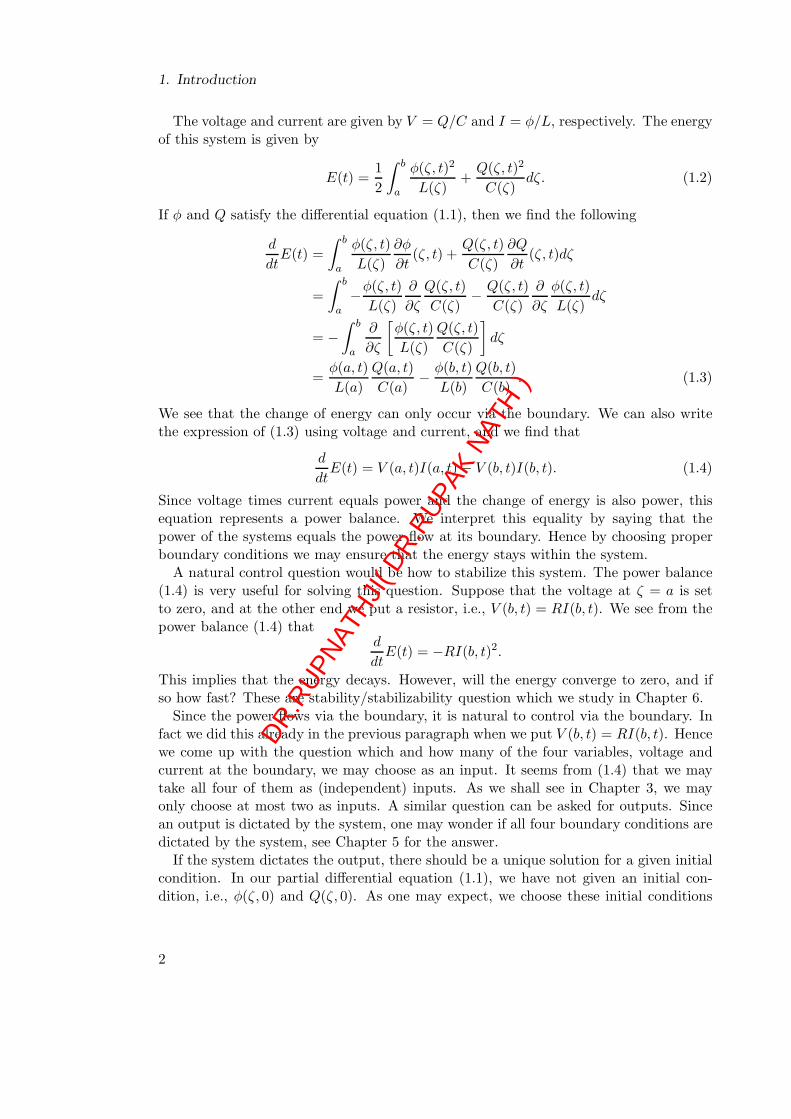
In this section we shall by using simple examples introduce our class and indicate whatare natural (control) questions for these systems. We begin with the example of thetransmission line. This model describes the charge density and magnetic flux in a cable,as is depictured below.

V (a)

I(a)

V (b)

I(b)a b

Figure 1.1.: Transmission line

Example 1.1.1 (Transmission line) Consider the transmission line on the spatialinterval [a, b]

∂Q

∂t(ζ, t) = − ∂

∂ζ

φ(ζ, t)

L(ζ)(1.1)

∂φ

∂t(ζ, t) = − ∂

∂ζ

Q(ζ, t)

C(ζ).

Here Q(ζ, t) is the charge at position ζ ∈ [a, b] and time t > 0, and φ(ζ, t) is the fluxat position ζ and time t. C is the (distributed) capacity and L is the (distributed)inductance.

1

DR.RUPN

ATHJI(

DR.R

UPAK

NATH )

1. Introduction

The voltage and current are given by V = Q/C and I = φ/L, respectively. The energyof this system is given by

E(t) =1

2

∫ b

a

φ(ζ, t)2

L(ζ)+Q(ζ, t)2

C(ζ)dζ. (1.2)

If φ and Q satisfy the differential equation (1.1), then we find the following

d

dtE(t) =

∫ b

a

φ(ζ, t)

L(ζ)

∂φ

∂t(ζ, t) +

Q(ζ, t)

C(ζ)

∂Q

∂t(ζ, t)dζ

=

∫ b

a−φ(ζ, t)

L(ζ)

∂

∂ζ

Q(ζ, t)

C(ζ)− Q(ζ, t)

C(ζ)

∂

∂ζ

φ(ζ, t)

L(ζ)dζ

= −∫ b

a

∂

∂ζ

[φ(ζ, t)

L(ζ)

Q(ζ, t)

C(ζ)

]dζ

=φ(a, t)

L(a)

Q(a, t)

C(a)− φ(b, t)

L(b)

Q(b, t)

C(b). (1.3)

We see that the change of energy can only occur via the boundary. We can also writethe expression of (1.3) using voltage and current, and we find that

d

dtE(t) = V (a, t)I(a, t) − V (b, t)I(b, t). (1.4)

Since voltage times current equals power and the change of energy is also power, thisequation represents a power balance. We interpret this equality by saying that thepower of the systems equals the power flow at its boundary. Hence by choosing properboundary conditions we may ensure that the energy stays within the system.

A natural control question would be how to stabilize this system. The power balance(1.4) is very useful for solving this question. Suppose that the voltage at ζ = a is setto zero, and at the other end we put a resistor, i.e., V (b, t) = RI(b, t). We see from thepower balance (1.4) that

d

dtE(t) = −RI(b, t)2.

This implies that the energy decays. However, will the energy converge to zero, and ifso how fast? These are stability/stabilizability question which we study in Chapter 6.

Since the power flows via the boundary, it is natural to control via the boundary. Infact we did this already in the previous paragraph when we put V (b, t) = RI(b, t). Hencewe come up with the question which and how many of the four variables, voltage andcurrent at the boundary, we may choose as an input. It seems from (1.4) that we maytake all four of them as (independent) inputs. As we shall see in Chapter 3, we mayonly choose at most two as inputs. A similar question can be asked for outputs. Sincean output is dictated by the system, one may wonder if all four boundary conditions aredictated by the system, see Chapter 5 for the answer.

If the system dictates the output, there should be a unique solution for a given initialcondition. In our partial differential equation (1.1), we have not given an initial con-dition, i.e., φ(ζ, 0) and Q(ζ, 0). As one may expect, we choose these initial conditions

2

DR.RUPN

ATHJI(

DR.R

UPAK

NATH )

1.1. Motivating examples

in the energy space, meaning that the initial energy, E(0), is finite. Giving only aninitial condition is not sufficient for a partial differential equation (p.d.e.) to have a(unique) solution, one also has to impose boundary conditions. In Chapter 2 we answerthe technical question for which boundary conditions the p.d.e. possesses a (unique)solution.

The previous example is standard for the class of systems we are studying. Thereis an energy function (Hamiltonian), a power balance giving that the change of energy(power) goes via the boundary of the spatial domain. The example of the (undamped)vibrating string is very similar.

Example 1.1.2 (Wave equation) Consider a vibrating string of length L = b − a,held stationary at both ends and free to vibrate transversely subject to the restoringforces due to tension in the string. The vibrations on the system can be modeled by

∂2w

∂t2(ζ, t) = c

∂2w

∂ζ2(ζ, t), c =

T

ρ, t ≥ 0, (1.5)

where ζ ∈ [a, b] is the spatial variable, w(ζ, t) is the vertical position of the string, Tis the Young’s modulus of the string, and ρ is the mass density, which are assumedto be constant along the string. This model is a simplified version of other systemswhere vibrations occur, as in the case of large structures, and it is also used in acoustics.Although the wave equation is normally presented in the form (1.5), it is not the formwe will be using. However, more importantly, it is not the right model when Young’smodulus or the mass density are depending on the spatial coordinate. When the laterhappens, the correct model is given by

∂2w

∂t2(ζ, t) =

1

ρ(ζ)

∂

∂ζ

[T (ζ)

∂w

∂ζ(ζ, t)

]. (1.6)

It is easy to see that this equals (1.5) when the physical parameter are not spatiallydependent. This system has the energy/Hamiltonian

E(t) =1

2

∫ b

aρ(ζ)

(∂w

∂t(ζ, t)

)2

+ T (ζ)

(∂w

∂ζ(ζ, t)

)2

dζ. (1.7)

As we did in the previous example we can calculate the change of energy, i.e., power.This gives (see also Exercise 1.1)

d

dtE(t) =

∂w

∂t(b, t)T (b)

∂w

∂ζ(b, t) − ∂w

∂t(a, t)T (a)

∂w

∂ζ(a, t). (1.8)

Again we see that the change of energy goes via the boundary of the spatial domain.One may notice that the position is not the (actual) variable used in the energy and thepower expression. The variables are velocity (∂w∂t ) and strain (∂w∂ζ ).

For this model one can pose similar questions as for the model from Example 1.1.1.In particular, a control problem could be to damp out the vibrations on the string.One approach to do this is to add damping along the spatial domain. This can also bedone by interacting with the forces and velocities at the end of the string, i.e., at theboundary.

3

DR.RUPN

ATHJI(

DR.R

UPAK

NATH )

1. Introduction

Example 1.1.3 (Beam equations) In recent years the boundary control of flexiblestructures has attracted much attention with the increase of high technology applicationssuch as space science and robotics. In these applications the control of vibrations iscrucial. These vibrations can be modeled by beam equations. For instance, the Euler-Bernoulli beam equation models the transversal vibration of an elastic beam if the cross-section dimension of the beam is negligible in comparison with its length. If the cross-section dimension is not negligible, then it is necessary to consider the effect of the rotaryinertia. In that case, the transversal vibration is better described by the Rayleigh beamequation. An improvement over these models is given by the Timoshenko beam, since itincorporates shear and rotational inertia effects, which makes it a more precise model.These equations are given, respectively, by

• Euler-Bernoulli beam:

ρ(ζ)∂2w

∂t2(ζ, t) +

∂2

∂ζ2

(EI(ζ)

∂2w

∂ζ2(ζ, t)

)= 0, ζ ∈ (a, b), t ≥ 0,

where w(ζ, t) is the transverse displacement of the beam, ρ(ζ) is the mass per unitlength, E(ζ) is the Young’s modulus of the beam, and I(ζ) is the area moment ofinertia of the beam’s cross section.

• Rayleigh beam:

ρ(ζ)∂2w

∂t2(ζ, t) − Iρ(ζ)

∂2

∂t2

(∂2w

∂ζ2(ζ, t)

)+

∂2

∂ζ2

(EI(ζ)

∂2w

∂z2(ζ, t)

)= 0,

where ζ ∈ (a, b), t ≥ 0, w(ζ, t) is the transverse displacement of the beam, ρ(ζ)is the mass per unit length, Iρ is the rotary moment of inertia of a cross section,E(ζ) is the Young’s modulus of the beam, and I(ζ) is the area moment of inertia.

• Timoshenko beam:

ρ(ζ)∂2w

∂t2(ζ, t) =

∂

∂ζ

[K(ζ)

(∂w

∂ζ(ζ, t) − φ(ζ, t)

)], ζ ∈ (a, b), t ≥ 0,

(1.9)

Iρ(ζ)∂2φ

∂t2(ζ, t) =

∂

∂ζ

(EI(ζ)

∂φ

∂ζ(ζ, t)

)+K(ζ)

(∂w

∂ζ(ζ, t) − φ(ζ, t)

),

where w(ζ, t) is the transverse displacement of the beam and φ(ζ, t) is the rotationangle of a filament of the beam. The coefficients ρ(ζ), Iρ(ζ), E(ζ), I(ζ), and K(ζ)are the mass per unit length, the rotary moment of inertia of a cross section,Young’s modulus of elasticity, the moment of inertia of a cross section, and theshear modulus respectively.

For the last model we show that it has similar properties as found in the previousexamples. The energy/Hamiltonian for this system is given by

E(t) =1

2

∫ b

a

[K(ζ)

(∂w

∂ζ(ζ, t) − φ(ζ, t)

)2

+ ρ(ζ)

(∂w

∂t(ζ, t)

)2

+

E(ζ)I(ζ)

(∂φ

∂ζ(ζ, t)

)2

+ Iρ

(∂φ

∂t(ζ, t)

)2]dζ. (1.10)

4

DR.RUPN

ATHJI(

DR.R

UPAK

NATH )

1.1. Motivating examples

Next we want to calculate the power. For this it is better to introduce some (physical)notation first.

x1(ζ, t) =∂w

∂ζ(ζ, t) − φ(ζ, t) shear displacement

x2(ζ, t) = ρ(ζ)∂w

∂t(ζ, t) momentum

x3(ζ, t) =∂φ

∂ζ(ζ, t) angular displacement

x4(ζ, t) = Iρ(ζ)∂φ

∂t(ζ, t) angular momentum

Using this notation and the model (1.9), we find that the power equals (Exercise 1.2)

dE

dt(t) =

[K(ζ)x1(ζ, t)

x2(ζ, t)

ρ(ζ)+ E(ζ)I(ζ)x3(ζ, t)

x4(ζ, t)

Iρ(ζ)

]b

a

. (1.11)

Again we see that the power goes via the boundary of the spatial domain.

In the previous three examples we see that by imposing the right-boundary conditionsno energy will be lost. In other words, these system cannot loose energy internally.However, there are many systems in which there is (internal) loss of energy. This maybe caused by internal friction by internal friction, as is the case in the following example.

Example 1.1.4 (Damped wave equation) Consider the one-dimensional wave equa-tion of Example 1.1.2. One cause of damping is known as structural damping. Struc-tural damping arises from internal friction in a material converting vibrational energyinto heat. In this case the vibrating string is modeled by

∂2w

∂t2(ζ, t) =

1

ρ(ζ)

∂

∂ζ

[T (ζ)

∂w

∂ζ(ζ, t)

]+

ksρ(ζ)

∂2

∂ζ2

[∂w

∂t(ζ, t)

], ζ ∈ [a, b], t ≥ 0, (1.12)

where ks is a positive constant.

To see that the energy decays, we calculate the power, i.e., dEdt , where the energy is

given by (1.7).

d

dtE(t) =

∂w

∂t(b, t)T (b)

∂w

∂ζ(b, t) − ∂w

∂t(a, t)T (a)

∂w

∂ζ(a, t) + (1.13)

∂w

∂t(b, t)ks

∂2w

∂ζ∂t(b, t) − ∂w

∂t(a, t)ks

∂2w

∂ζ∂t(a, t) − ks

∫ b

a

[∂2w

∂ζ∂t(ζ, t)

]2

dζ.

From this equality, we see that if there is no energy flow through the boundary, theenergy will still decay.

Although this system looses energy internally, questions like is the system decaying tozero, when no force is applied at the boundary are still valid for this model as well.

The most standard example of a model with diffusion, is the model of heat distribution.

5

DR.RUPN

ATHJI(

DR.R

UPAK

NATH )

1. Introduction

Example 1.1.5 (Heat conduction) The model of heat conduction consists of onlyone conservation law, that is the conservation of energy. It is given by the followingconservation law:

∂u

∂t= − ∂

∂ζJQ, (1.14)

where u(ζ, t) is the energy density and JQ(ζ, t) is the heat flux. This conservation law iscompleted by two closure equations. The first one expresses the calorimetric propertiesof the material:

∂u

∂T= cV (T ), (1.15)

where T (ζ, t) is the temperature distribution and cV is the heat capacity. The secondclosure equation defines heat conduction property of the material (Fourier’s conductionlaw):

JQ = −λ(T, ζ)∂T

∂ζ, (1.16)

where λ(T, ζ) denotes the heat conduction coefficient. Assuming that the variations ofthe temperature are not too large, one may assume that the heat capacity and the heatconduction coefficient are independent of the temperature, one obtains the followingpartial differential equation:

∂T

∂t=

1

cV

∂

∂ζ

(λ(ζ)

∂T

∂ζ

). (1.17)

If we look at the (positive) quantity E(t) = 12

∫ ba cV T (ζ, t)2dζ, then it is not hard to see

thatdE

dt(t) =

[T (ζ, t)λ(ζ)

∂T

∂ζ(ζ, t)

]b

a

−∫ b

aλ(ζ)

(∂T

∂ζ(ζ, t)

)2

dζ.

Hence even when there is no heat flow through the boundary of the spatial domain, thequantity E(t) will decrease. It will decrease as long as the heat flux is non-zero.

This later two examples are in nature completely different to the first examples. In thenext section we show that the first three examples have a common format. We returnto the example of the structural damped wave and the heat conduction only in Chapter7 of these notes.

1.2. Class of PDE’s

In this section we revisit the first examples of the previous section and show that theyall lie in the same class of systems.

If we introduce the variable x1 = Q and x2 = φ in the first example, see equation(1.1), then the p.d.e. can be written as

∂

∂t

(x1(ζ, t)x2(ζ, t)

)=

(0 −1−1 0

)∂

∂ζ

[(1

C(ζ) 0

0 1L(ζ)

)(x1(ζ, t)x2(ζ, t)

)]. (1.18)

6

DR.RUPN

ATHJI(

DR.R

UPAK

NATH )

1.2. Class of PDE’s

The Hamiltonian is written as, see (1.2)

E(t) =1

2

∫ b

a

x1(ζ, t)2

C(ζ)+x2(ζ, t)

2

L(ζ)dζ

=1

2

∫ b

a

(x1(ζ, t) x2(ζ, t)

)(

1C(ζ) 0

0 1L(ζ)

)(x1(ζ, t)x2(ζ, t)

)dζ. (1.19)

For the wave equation we can write down a similar form. We define x1 = ρ∂w∂t (momen-

tum) and x2 = ∂w∂ζ (strain). The p.d.e. (1.6) can equivalently be written as

∂

∂t

(x1(ζ, t)x2(ζ, t)

)=

(0 11 0

)∂

∂ζ

[( 1ρ(ζ) 0

0 T (ζ)

)(x1(ζ, t)x2(ζ, t)

)]. (1.20)

The energy/Hamiltonian becomes in the new variables, see (1.7),

E(t) =1

2

∫ b

a

x1(ζ, t)2

ρ(ζ)+ T (ζ)x2(ζ, t)

2dζ

=1

2

∫ b

a

(x1(ζ, t) x2(ζ, t)

)( 1ρ(ζ) 0

0 T (ζ)

)(x1(ζ, t)x2(ζ, t)

)dζ. (1.21)

For the model of Timoshenko beam, we have already introduced our variables in Example1.1.3. We write the model and the energy using these new variables. Calculating thetime derivative of the variables x1, . . . , x4, we find by using (1.9)

∂

∂t

x1(ζ, t)x2(ζ, t)x3(ζ, t)x4(ζ, t)

=

∂∂ζ

(x2(ζ,t)ρ(ζ)

)− x4(ζ,t)

Iρ(ζ)∂∂z (K(ζ)x1(ζ, t))∂∂z

(x4(ζ,t)Iρ(ζ)

)

∂∂z (E(ζ)I(ζ)x3(ζ, t)) +K(ζ)x1(ζ, t)

(1.22)

We can write this in a form similar to those presented in (1.18) and (1.20). However, aswe shall see, we also need a “constant” term. Since this is a long expression, we will notwrite down the coordinates ζ and t.

∂

∂t

x1

x2

x3

x4

=

0 1 0 01 0 0 00 0 0 10 0 1 0

∂

∂ζ

K 0 0 00 1

ρ 0 0

0 0 EI 00 0 0 1

Iρ

x1

x2

x3

x4

+

0 0 0 −10 0 0 00 0 0 01 0 0 0

K 0 0 00 1

ρ 0 0

0 0 EI 00 0 0 1

Iρ

x1

x2

x3

x4

. (1.23)

7

DR.RUPN

ATHJI(

DR.R

UPAK

NATH )

1. Introduction

Formulating the energy/Hamiltonian in the variables x1, . . . , x4 is easier, see (1.10)

E(t) =1

2

∫ b

aK(ζ)x1(ζ, t)

2 +1

ρ(ζ)x2(ζ, t)

2 +E(ζ)I(ζ)x3(ζ, t)2 +

1

Iρ(ζ)x4(ζ, t)

2dζ

=1

2

∫ b

a

x1(ζ, t)x2(ζ, t)x3(ζ, t)x4(ζ, t)

T

K(ζ) 0 0 00 1

ρ(ζ) 0 0

0 0 E(ζ)I(ζ) 00 0 0 1

Iρ(ζ)

x1(ζ, t)x2(ζ, t)x3(ζ, t)x4(ζ, t)

dζ.

(1.24)

We see that in the new formulation these examples have a common structure. There isonly one spatial and one time derivative, and the relation between these two derivativesis of the form

∂x

∂t(ζ, t) = P1

∂

∂ζ[H(ζ)x(ζ, t)] + P0 [H(ζ)x(ζ, t)] . (1.25)

Furthermore, we have that P1 is symmetric, i.e., P T1 = P1, P0 is anti-symmetric, i.e.,P T0 = −P0. Furthermore, they are both independent of ζ. Finally, H is a (strictly)positive symmetric multiplication operator, independent of t. The energy or Hamiltoniancan be expressed by using x and H. That is

E(t) =1

2

∫ b

ax(ζ, t)TH(ζ)x(ζ, t)dζ. (1.26)

As we have seen in the examples, the change of energy (power) of these systems was onlypossible via the boundary of its spatial domain. In the following theorem we show thatthis is a general property for any system which is of the form (1.25) with Hamiltonian(1.26).

Theorem 1.2.1. Consider the partial differential equation (1.25) in which P0, P1 areconstant matrices satisfying P T1 = P1 and P T0 = −P0. Furthermore, H is independenton t and is symmetric, i.e. for all ζ’s we have that H(ζ)T = H(ζ). For the Hamil-tonian/energy given by (1.26) the following balance equation holds for all solutions of(1.25)

dE

dt(t) =

1

2

[(Hx)T (ζ, t)P1 (Hx) (ζ, t)

]ba. (1.27)

Proof: By using the partial differential equation, we find that

dE

dt(t) =

1

2

∫ b

a

∂x

∂t(ζ, t)TH(ζ)x(ζ, t)dζ +

1

2

∫ b

ax(ζ, t)TH(ζ)

∂x

∂t(ζ, t)dζ

=1

2

∫ b

a

[P1

∂

∂ζ(Hx) (ζ, t) + P0 (Hx) (ζ, t)

]TH(ζ)x(ζ, t)dζ+

1

2

∫ b

ax(ζ, t)TH(ζ, t)

[P1

∂

∂ζ(Hx) (ζ, t) + P0 (Lx) (ζ, t)

]dζ.

8

DR.RUPN

ATHJI(

DR.R

UPAK

NATH )

1.3. Dirac structures and port-Hamiltonian systems

Using now the fact that P1,H(ζ) are symmetric, and P0 is anti-symmetric, we write thelast expression as

1

2

∫ b

a

[∂

∂ζ(Hx) (ζ, t)

]TP1H(ζ)x(ζ, t) + [H(ζ)x(ζ, t)]T

[P1

∂

∂ζ(Hx) (ζ, t)

]dζ+

1

2

∫ b

a− [H(ζ)x(ζ, t)]T P0H(ζ)x(ζ, t) + [H(ζ)x(ζ, t)]T [P0H(ζ)x(ζ, t)] dζ

=1

2

∫ b

a

∂

∂ζ

[(Hx)T (ζ, t)P1 (Hx) (ζ, t)

]dζ

=1

2

[(Hx)T (ζ, t)P1 (Hx) (ζ, t)

]ba.

Hence we have proved the theorem.

The balance equation will turn out to be very important, and will guide us in manyproblems. An overview of the (control) problems which we study in the coming chaptersis given in Section 1.4. First we concentrate a little bit more on the class of systemsgiven by (1.25). We show that we have to see it as a combination of two structure.One given by P1 and P0, and the other given by H. This is the subject of the followingsection, in which we also explain the name Port-Hamiltonian.

1.3. Dirac structures and port-Hamiltonian systems

In this section we show that we can identify a deeper underlying structure to the p.d.e.(1.25) and the balance equation (1.27). Therefore we look once more at the first displayedequation in the proof of Theorem 1.2.1. For a = −∞ and b = ∞ this equation becomes

dE

dt(t) =

1

2

∫ ∞

−∞

∂x

∂t(ζ, t)TH(ζ)x(ζ, t)dζ +

1

2

∫ ∞

−∞x(ζ, t)TH(ζ)

∂x

∂t(ζ, t)dζ. (1.28)

In the expression on the right-hand side we have ∂x∂t and Hx. These are the same variables

used to describe the p.d.e. (1.25). Let us rename these variables f = ∂x∂t and e = Hx.

Furthermore, we “forget” the time, i.e., we see e and f only as functions of the spatialvariable. By doing so the p.d.e. becomes

f(ζ) = P1∂e

∂ζ(ζ) + P0e(ζ) (1.29)

and the right-hand side of (1.28) becomes

1

2

∫ ∞

−∞f(ζ)T e(ζ)dζ +

1

2

∫ ∞

−∞e(ζ)T f(ζ)dζ. (1.30)

9

DR.RUPN

ATHJI(

DR.R

UPAK

NATH )

1. Introduction

Using the equation (1.29), we can rewrite the integrals in (1.30).

1

2

∫ ∞

−∞f(ζ)T e(ζ)dζ +

1

2

∫ ∞

−∞e(ζ)T f(ζ)dζ

=1

2

∫ ∞

−∞

[P1∂e

∂ζ(ζ) + P0e(ζ)

]Te(ζ)dζ+

1

2

∫ ∞

−∞e(ζ)T

[P1∂e

∂ζ(ζ) + P0e(ζ)

]dζ

=1

2

∫ ∞

−∞

∂e

∂ζ(ζ)TP1e(ζ) + e(ζ)TP1

∂e

∂ζ(ζ)dζ

=1

2

∫ ∞

−∞−e(ζ)TP0e(ζ) + e(ζ)TP0e(ζ)dζ

=1

2

∫ ∞

−∞

∂

∂ζ

[e(ζ)TP1e(ζ)

]dζ,

where we have used that P T1 = P1 and P T0 = −P0. We remark that the above derivationis exactly the same as the one in the proof of Theorem 1.2.1. Now under the mildassumption that e(ζ) is zero in plus and minus infinity, we conclude that

1

2

∫ ∞

−∞f(ζ)T e(ζ)dζ +

1

2

∫ ∞

−∞e(ζ)T f(ζ)dζ = 0. (1.31)

for all e and f satisfying (1.29).Based on (1.28) we call the expressions

∫fT edζ,

∫eT fdζ, the power. Remember that

the change of energy is by definition the power. Hence we see from (1.31) that the poweris zero. This was already clear from the proof of Theorem 1.2.1, but we received it nowfor any pair of variables which satisfies (1.29).

To illustrate this observation we consider three systems which have the same P1 andP0, but are totally different in their time behavior.

Example 1.3.1 We consider the following simple p.d.e.

∂x

∂t(ζ, t) =

∂x

∂ζ(ζ, t), ζ ∈ R. (1.32)

We regard this equation as the equation (1.29) with P1 = 1 and P0 = 0 and f = ∂x∂t ,

e = x. Hence if we define the energy E(t) = 12

∫∞−∞ x(ζ, t)2dζ and we assume that

x(±∞, t) = 0, then we know that E(t) is zero along solutions.

Example 1.3.2 Consider the following p.d.e.

∂x

∂t(ζ, t) = x(ζ, t)

∂x

∂ζ(ζ, t), ζ ∈ R. (1.33)

This equation is known as the inviscid Burgers’s equation. If we define f = ∂x∂t and

e = 12x

2, then we see that this equation equals (1.29) for the same P1 and P0 as in the

10

DR.RUPN

ATHJI(

DR.R

UPAK

NATH )

1.3. Dirac structures and port-Hamiltonian systems

previous example. Furthermore, we know that

0 = 2

∫ ∞

−∞f(ζ, t)e(ζ, t)dζ =

∫ ∞

−∞

∂x

∂t(ζ, t)x(ζ, t)2dζ

provided x(∞, t) = x(−∞, t) = 0 for all t. The later integral can see as the timederivative of H(t) = 1

3

∫∞−∞ x(ζ, t)3dζ. Hence we find that this H is a conserved quantity,

i.e.,dH

dt(t) = −

∫ ∞

−∞

∂x

∂t(ζ, t)x(ζ, t)2dζ =

∫ ∞

−∞f(ζ, t)e(ζ, t)dζ = 0. (1.34)

The above holds for every x satisfying (1.33) with x(∞, t) = x(−∞, t) = 0. Sincethe p.d.e. (1.33) is non-linear, proving existence of solutions is much harder than inthe previous example. However, as in the linear example we have found a conservedquantity.

In the previous example we have chosen a different e, but the same f . We can alsochoose a different f .

Example 1.3.3 Consider the discrete-time implicit equation

x(ζ, n+ 1) − x(ζ, n) =∂

∂ζ[x(ζ, n+ 1) + x(ζ, n)] , ζ ∈ R, n ∈ Z. (1.35)

In this equation, we choose f(ζ, n) = x(ζ, n+1)−x(ζ, n) and e(ζ, n) = x(ζ, n+1)+x(ζ, n).For this choice, we see that (1.35) is the same as (1.29) with P1 = 1 and P0 = 0.

If we choose the energy to be same as in Example 1.3.1, i.e., E(n) =∫∞−∞ x(ζ, n)2dζ,

then we find that

E(n+ 1) − E(n) =

∫ ∞

−∞x(ζ, n+ 1)2 − x(ζ, n)2dζ =

∫ ∞

−∞f(ζ, n)e(ζ, n)dζ = 0, (1.36)

provided x(±∞, n) = 0 for all n ∈ Z. So for the implicit difference equation (1.35) wehave once more a conserved quantity without knowing the solutions, or even knowingexistence.

As is become clear in the previous examples we may distinguish between an underlyingstructure and the actual system. This underlying structure is named a Dirac structureand is defined next.

Definition 1.3.4. Let E and F be two Hilbert spaces with inner product 〈·, ·〉E and〈·, ·〉F , respectively. Assume moreover that they are isometrically isomorphic, that isthere exists a linear mapping rF ,E : F 7→ E such that

〈rF ,Ef1, rF ,Ef2〉E = 〈f1, f2〉F (1.37)

for all f1, f2 ∈ F . The bond space B is defined as F × E . On B we define the followingsymmetric pairing

⟨(f1

e1

),

(f2

e2

)⟩

+

= 〈f1, rE,Fe2〉F + 〈e1, rF ,Ef2〉E , (1.38)

11

DR.RUPN

ATHJI(

DR.R

UPAK

NATH )

1. Introduction

where rE,F = r−1F ,E .

Let V be a linear subspace of B, then the orthogonal subspace with respect to thesymmetric pairing (1.38) is defined as

V⊥ = b ∈ B | 〈b, v〉+ = 0 for all v ∈ V. (1.39)

A Dirac structure is a linear subspace of the bond space D satisfying

D⊥ = D. (1.40)

♣The variables e and f are called the effort and flow , respectively, and their spaces E

and F are called the effort and flow space. The bilinear product 〈f, rE,Fe〉F is called thepower or power product . Note that 〈f, rE,Fe〉F = 〈rF ,Ef, e〉E .

Dirac structures are depictured in Figure 1.2. Finally, we mention that by (1.39), we

f

e

D

Figure 1.2.: Dirac structure

have that for any element of the Dirac structure

2〈f, rE,Fe〉F = 〈b, b〉+ = 0. (1.41)

This we interpret by saying that for any element of a Dirac structure the power is zero.A Dirac structure can been seen as the largest subspace which this holds i.e., if V is asubspace of B satisfying (1.41), then V is a Dirac structure if there does not exists asubspace W such that V ⊂ W, V 6= W, and the power of every element in W is zero.

Next we identify the Dirac structure associated to Examples 1.3.1–1.3.3.

Example 1.3.5 Choose the effort and flow space as L2(−∞,∞), and let rF ,E = I.Define the following subspace of B = F × E

D =

(fe

)∈ B | e is absolutely continuous and

de

dζ∈ L2(−∞,∞), (1.42)

e(−∞) = e(∞) = 0, and f =de

dζ

.

We claim that this subspace is a Dirac structure. Let b = ( fe ) ∈ B and let 〈b, d〉+ = 0for all d =

(fded

)∈ D. Using our power product this implies that

0 = 〈f, ed〉 + 〈fd, e〉 = 〈f, ed〉 + 〈deddζ

, e〉.

12

DR.RUPN

ATHJI(

DR.R

UPAK

NATH )

1.3. Dirac structures and port-Hamiltonian systems

In other words

〈deddζ

, e〉 = −〈ed, f〉. (1.43)

This is equivalent to saying that e lies in the domain of the dual of the differentialoperator, d

dζ . Similar to Example A.3.64 and A.3.66 we conclude from this equationthat e is absolutely continuous and e(−∞) = e(∞) = 0. Furthermore, by integration byparts we see that

〈deddζ

, e〉 =

∫ ∞

−∞

deddζ

(ζ)e(ζ)dζ = −∫ ∞

−∞ed(ζ)

de

dζ(ζ)dζ = −〈ed,

de

dζ〉.

Combining this with (1.43), we conclude that

−〈ed,de

dζ〉 = −〈ed, f〉.

Since this holds for a dense set of ed, we conclude that f = dedζ . Concluding, we see that

( fe ) ∈ D, and so D is a Dirac structure.

Now we have formally defined what is a Dirac structure, we can define our class ofsystems.

Let H be a real-valued function of x, and let D be a Dirac structure. We furthermoreassume that we have a mapping H from F to R which is Frechet differentiable for anyx, i.e., see Definition A.5.25.

H(x+ ∆x) −H(x) = (dH(x)) (∆x) +R(x,∆x), (1.44)

with ‖R(x,∆x)‖‖∆x‖ converges to zero when ∆x → 0. Since H takes values in R, we can by

Riesz representation theorem write the term (dH(x)) (∆x) as 〈∆x, f〉F for some f . Notethat f still depends on x. Since F is isomorphically isomorf to E , we can find an e suchthat 〈∆x, f〉F = 〈∆x, rE,F e〉F . We denote this e by ∂H

∂x (x). Combining this notationwith equation (1.44), we find

H(x+ ε∆x) −H(x) = ε〈∆x, rE,F∂H

∂x(x)〉F + εo(ε). (1.45)

The system associated with H and D is defined as

x(·, t) |(

∂x∂t (·, t)∂H

∂x (·, t)

)∈ D for all t. (1.46)

Before we write our examples in this format, we show that the system defined above hasH as a conserved quantity along its trajectory.

H(x(t+ ε)) −H(x(t)) = H (x(t) + εx(t) + εr(x(t), ε)) −H(x(t)),

13

DR.RUPN

ATHJI(

DR.R

UPAK

NATH )

1. Introduction

where ‖r(x(t), ε)‖ → 0 when ε → 0. Since ε is small, we may ignore this term. Doingso, and using (1.45) we find

H(x(t+ ε)) −H(x(t))

ε= 〈x(t), rE,F

∂H

∂x(x(t))〉F + o(ε).

By the definition of our system, we have that the power product is zero, see (1.41) andso, we find that

dH(x(t))

dt= 0.

Note that we normally write H(t) instead of H(x(t)). Thus along trajectories, H is aconserved quantity. This conserved quantity is called the Hamiltonian. Equation (1.46)clearly indicates that the system is defined by two objects. Namely, the Dirac structureand the Hamiltonian.

We illustrate the above by looking once more to the Examples 1.3.1 and 1.3.2.

Example 1.3.6 From Example 1.3.5 we know which Dirac structure lies under thep.d.e.’s of Examples 1.3.1 and 1.3.2. Hence it remains to identify the Hamiltonians.

For Example 1.3.1 we easily see that H = 12

∫∞−∞ x2dζ. If we define H = 1

2x2, then it

by combining (1.46) with (1.42) gives the p.d.e. (1.32).For Example 1.3.2 we find H = 1

3

∫∞−∞ x3dζ and H = 1

3x3.

In contrast to our examples in Section 1.1, the examples 1.3.1–1.3.3 do not have aboundary. However, as seen in e.g. Example 1.1.1 the boundary is very useful for controlpurposes. So we have to re-think and adjust the theory as developed until now. Toillustrate this, we consider Example 1.3.3 on a compact spatial interval.

Example 1.3.7 Consider the p.d.e.

∂x

∂t(ζ, t) =

∂x

∂ζ(ζ, t), ζ ∈ (a, b). (1.47)

As in Theorem 1.2.1,we take the energy equal to E(t) = 12

∫ ba x(ζ, t)

2dζ. We find that

dE

dt(t) =

∫ b

a

∂x

∂t(ζ, t)x(ζ, t)dζ =

1

2

[x(b, t)2 − x(a, t)2

]. (1.48)

Or equivalently,

dE

dt(t) =

∫ b

a

∂x

∂t(ζ, t)x(ζ, t)dζ − 1

2

[x(b, t)2 − x(a, t)2

]= 0. (1.49)

As before, we want to see the middle expression as a power product. Hence if weintroduce f = ∂x

∂t and e = x, then the integral induces a power product between f ande. However, we still have the boundary terms. We introduce the boundary port variablesf∂ = 1√

2[x(b) − x(a)], and e∂ = 1√

2[x(b) + x(a)]. With these variables, we see that we

may write (1.49) asdE

dt=

∫ b

af(ζ)e(ζ)dζ − f∂e∂ = 0. (1.50)

14

DR.RUPN

ATHJI(

DR.R

UPAK

NATH )

1.3. Dirac structures and port-Hamiltonian systems

We can see this as a system like (1.46) by defining

E = F = L2(a, b) ⊕ R

and

rF ,E =

(I 00 −1

).

The Dirac structure is given by

D =

ff∂ee∂

∈ B | e is absolutely continuous and

de

dζ∈ L2(a, b), (1.51)

f =de

dζ, f∂ =

1√2[e(b) − e(a)] and e∂ =

1√2[e(b) + e(a)].

Again we have a Dirac structure, but now it contains boundary variables. We canformulate our system on this Dirac structure as

x(·, t) |

∂x∂tf∂∂H

∂xe∂

∈ D. (1.52)

where D is given by (1.51) and H = 12x

2.

From (1.52) we see that our system is defined via a Dirac structure, an Hamiltonianand port variables. This motivated the name “Port-Hamiltonian Systems”.

One of the advantages of considering a system as a Dirac structure with a Hamiltonianis that coupling of systems is now very easy. Suppose we have two Dirac structures, D1

and D2 as depictured in Figure 1.3. We couple the structures by f2 = −f2 (the flow out

f1

e1

f2

e2

f1

e1

f2

e2

D1 D2

Figure 1.3.: Composition of Dirac structures

of the first system equals the incoming flow of the other system) and e2 = e2. Then thestructure defined by

D =

f1

f1

e1e1

| there exist f2, e2 s.t.

f1

f2

e1e2

∈ D1 and

f1

−f2

e1e2

∈ D2

. (1.53)

15

DR.RUPN

ATHJI(

DR.R

UPAK

NATH )

1. Introduction

has zero power. To see this, we assume that for both systems 〈f, e〉 + 〈e, f〉 denotes thepower. We take as power for D

〈f1, e1〉 + 〈e1, f1〉 + 〈f1, e1〉 + 〈e1, f1〉

We find for this power product

〈f1, e1〉 + 〈e1, f1〉+〈f1, e1〉 + 〈e1, f1〉= 〈f1, e1〉 + 〈e1, f1〉 + 〈f2, e2〉 + 〈e2, f2〉

− 〈f2, e2〉 − 〈e2, f2〉 + 〈f1, e1〉 + 〈e1, f1〉

=

⟨(f1

f2

),

(e1e2

)⟩+

⟨(e1e2

),

(f1

f2

)⟩+

⟨(f1

−f2

),

(e1e2

)⟩+

⟨(e1e2

),

(f1

−f2

)⟩.

The last expressions are zero since

(f1f2e1e2

)∈ D1 and

(f1−f2e1e2

)∈ D2, respectively. Thus

we see that the total power of the interconnected Dirac structure is zero. Although thisis not sufficient to show that D defined by (1.53) is a Dirac structure, it indicates thepromising direction. It only remains to show that D is maximal. For many coupledDirac structures this holds. If the systems has the Hamiltonian H1 and H2 respectively,then the Hamiltonian of the coupled system is H1 +H2. Of course we can extend thisto the coupling of more than two systems. We show a physical example next.

Example 1.3.8 (Suspension system) Consider a simplified version of a suspensionsystem described by two strings connected in parallel through a distributed spring. Thissystem can be modeled by

∂2u

∂t2=c2

∂2u

∂ζ2+ α(v − u) (1.54)

∂2v

∂t2=c2

∂2v

∂ζ2+ α(u− v) ζ ∈ (−∞, ∞), t ≥ 0,

where c and α are positive constants and u(ζ, t) and v(ζ, t) describe the displacement,respectively, of both strings. The use of this model has potential applications in isola-tion of objects from outside disturbances. As an example in engineering, rubber andrubber-like materials are used to absorb vibration or shield structures from vibration.As an approximation, these materials can be modeled as a distributed spring. We showthat this system can be described as the interconnection of three subsystems, i.e., twovibrating strings and one distributed spring. Seeing the system as an interconnection ofsubsystems allows us to have some modularity in the modeling process, and because ofthis modularity, the modeling process can be performed in an iterative manner, graduallyrefining the model by adding other subsystems.

16

DR.RUPN

ATHJI(

DR.R

UPAK

NATH )

1.4. Overview

1.4. Overview

Now we know the class of systems we will be working with we can give more details onthe content of the coming chapters.

In Chapter 2 we study for which homogenous boundary conditions the p.d.e. (1.25)possesses a unique solution which has non-increasing energy. This we do by applyingthe general theory of infinite-dimensional systems. If these boundary conditions are non-zero, then in Chapter 3 we show that this p.d.e. still has well-defined solutions. Hencethis enable us to apply a control (input) at the boundary to the system described by(1.25). Under this same conditions, we show that boundary output is also possible. Themapping between the input and the output can be described by the transfer function.This is the subject of Chapter 4. Till Chapter 5 we have only considered systems whichare non-increasing in energy if no control is applied. Furthermore, the control has beenrestricted to smooth functions. In Chapter 5, we extend our class of systems in bothdirections. We show that many more boundary conditions are possible, and furthermore,we show that if the homogenous system is well-posed, then the same hold for the systemwhen L2-input are applied. Chapter 6 we can solve our first control problem. We canidentify a large class of boundary feedback which stabilize the system. The stability isexponential, meaning that the energy decays exponentially fast to zero. In 7 we cantreat a larger class of system. There we return to the examples 1.1.4 and 1.1.5. In thissection, we really need the underlying Dirac structure. Hence till Chapter 7, the Diracstructure is underlying our system, and apart for using to define boundary port, we shallnot use it very prominently. This changes in Chapter 7.

1.5. Exercises

1.1. In this exercise we check some integrals which appeared in our examples.

a) Check equation (1.8).

b) Check the equality (1.13).

1.2. Prove equation (1.11).

1.3. Show that equation (1.51) in Example 1.3.7 defines a Dirac structure.

17

DR.RUPN

ATHJI(

DR.R

UPAK

NATH )

1. Introduction

18

DR.RUPN

ATHJI(

DR.R

UPAK

NATH )

Chapter 2

Homogeneous differential equation

2.1. Introduction

In this chapter we study the partial differential equation (1.25). In particular, we char-acterize boundary conditions such that this p.d.e. has a unique solution, and such thatthe energy decays along the solutions. In order to clarify the approach we take, let usconsider the most simplified version of (1.25)

∂x

∂t(ζ, t) = α

∂x

∂ζ(ζ, t), ζ ∈ [0, 1], t ≥ 0, (2.1)

where α is a positive constant. As initial condition we take x0(ζ).If x0 is continuously differentiable, then it is easy to see that a solution is given by,

see Exercise 2.1.

x(ζ, t) =

x0(ζ + αt) ζ ∈ [0, 1], ζ + αt < 1

x0(1) ζ ∈ [0, 1], ζ + αt > 1(2.2)

However, this is not the only solution of (2.1). Another solution is given by

x(ζ, t) =

x0(ζ + αt) ζ ∈ [0, 1], ζ + αt < 1

g(ζ + αt) ζ ∈ [0, 1], ζ + αt > 1(2.3)

where g is an arbitrary continuous differentiable function on (1,∞) satisfying g(1) =x0(1).

Hence we have that the p.d.e. does not possess a unique solution. The reason for thisis that we did not impose a boundary condition. If we impose the boundary conditionx(1, t) = 0 for all t, then the unique solution is given by, see also (2.2),

x(ζ, t) =

x0(ζ + αt) ζ ∈ [0, 1], ζ + αt < 1

0 ζ ∈ [0, 1], ζ + αt > 1(2.4)

Note that we assume that x0(1) satisfies the boundary condition as well. The rule ofthumb is that for a first order p.d.e. one need one boundary condition. However, this is

19

DR.RUPN

ATHJI(

DR.R

UPAK

NATH )

2. Homogeneous differential equation

only a rule of thumb. If we impose to the p.d.e. (2.1) the boundary condition x(0, t) = 0,then this p.d.e. does not possess any solution if x0 6= 0, see Exercise 2.2.

We return to the p.d.e. (2.1) with boundary condition x(1, t) = 0. The solution isgiven by (2.4). We see that for any initial condition, even the ones which are onlyintegrable, the function x(ζ, t) of (2.4) is well-defined. This function depends on x0. Inparticular, we can define mappings

x0 7→ x(·, t), t ≥ 0. (2.5)

This mapping has the following properties

• It is linear, i.e., if x0 is written as c1f0 + c2g0, then x can be written as c1f + c2g,where f0, g0 are mapped to f and g, respectively.

• If we take x1 equal to x(·, τ), then the (composed) mapping

x0 7→ x(·, τ) = x1 7→ x(·, t)

equals the mappingx0 7→ x(·, t+ τ).

The reason for these properties lies in the linearity and time-invariance of the p.d.e.Next we choose a (particular) class of initial conditions. It is easy to see that (2.1) is of

the form (1.25), and so the energy associated to it equals 12

∫ 10 |x(ζ)|2dζ, or 1

2

∫ 10 α|x(ζ)|2dζ.

We take the class of functions with finite energy to be our class of initial conditions.Thus we have defined for our simple example the space of initial conditions, and

we have seen some nice properties of the solution. In the sequel we omit the spatialargument, when we write down an initial condition, or a solution, and we see (2.5) as amapping in the energy space.

In the following section we first have to consider some abstract theory. The generalresult obtained there enables us to show that for certain boundary conditions the p.d.e.(1.25) possesses a unique solution.

2.2. Semigroup and infinitesimal generator

In this section, we recap some abstract differential theory. We denote by X an abstractHilbert space, with inner product 〈·, ·〉X and norm ‖ · ‖X =

√〈·, ·〉X . For the simple

p.d.e. considered in the previous section, we saw some nice properties of the mappingfrom the initial condition to the solution at time t. These properties are formalized inthe following definition.

Definition 2.2.1. Let X be a Hilbert space. The operator valued function t 7→ T (t),t ≥ 0 is a strongly continuous semigroup if the following holds

1. For all t ≥ 0, T (t) is a bounded linear operator on X, i.e., T (t) ∈ L(X);

2. T (0) = I;

20

DR.RUPN

ATHJI(

DR.R

UPAK

NATH )

2.2. Semigroup and infinitesimal generator

3. T (t+ τ) = T (t)T (τ) for all t, τ ≥ 0.

4. For all x0 ∈ X, we have that ‖T (t)x0 − x0‖X converges to zero, when t ↓ 0.

We sometimes abbreviate strongly continuous semigroup to C0-semigroup and mosttimes it will be denoted by (T (t))t≥0. ♣

We call X the state space, and its elements states. To obtain a feeling for these definingproperties assume that T (t) denotes the mapping of initial condition to solution at timet of some linear, time-invariant, differential equation. We remark that this will alwayshold for any semigroup, see Lemma 2.2.6. Under this assumption, we can understandthese defining properties of a strongly continuous semigroup much better.

1. That T (t) is a bounded operator means that the solution at time t has not leftthe space of initial conditions, i.e., the state space. The linearity implies that thesolution corresponding to the initial condition x0 + x0 equals x(t) + x(t), wherex(t) and x(t) are the solution corresponding to x0 and x0, respectively. This islogical, because we assumed that the underlying differential equation is linear.

2. This is trivial; the solution at time zero must be equal to the initial condition.

3. Let x(τ) be the state at time τ . If we take this as our new initial condition andproceed for t seconds, then by the time-invariance this must equal x(t+τ). Since weassume that T (s) is the mapping from x0 to x(s), we see that the time-invarianceof the underlying differential equation implies property 3. of Definition 2.2.1.

Property 3. is known as a group property, and since it only holds for positive time,it motivates the name “semigroup”.

4. This property tells you that if you go backward in time to zero, then x(t) ap-proaches the initial condition. This sounds very logical, but need not to hold forall operators satisfying 1.–3.

Property 4. is known as strong continuity.

The easiest example of a strongly continuous semigroup is the exponential of a matrix.That is, let A be an n × n matrix, the matrix-valued function T (t) = eAt satisfies theproperties of Definition 2.2.1 on the Hilbert space Rn, see Exercise 2.3. Clearly theexponential of a matrix is also defined for t < 0. If the semigroup can be extended toall t ∈ R, then we say that T (t) is a group. We present the formal definition next.

Definition 2.2.2. Let X be a Hilbert space. The operator valued function t 7→ T (t),t ∈ R is a strongly continuous group, or C0-group, if the following holds

1. For all t ∈ R, T (t) is a bounded linear operator on X;

2. T (0) = I;

3. T (t+ τ) = T (t)T (τ) for all t, τ ∈ R.

21

DR.RUPN

ATHJI(

DR.R

UPAK

NATH )

2. Homogeneous differential equation

4. For all x0 ∈ X, we have that ‖T (t)x0 − x0‖X converges to zero, when t→ 0. ♣

It is easy to see that the exponential of a matrix is a group. However, only a fewsemigroups are actually a group. In the study of p.d.e.’s you encounter semigroups moreoften than groups. The reason for that is that if you have a group, you may go fromthe initial condition backward in time. For our simple p.d.e. of Section 2.1 this is notpossible, as it is shown at the end of the following example.

Example 2.2.3 In this example we show that the mapping defined by (2.5) defines astrongly continuous semigroup. As state space we choose L2(0, 1). We see that its normcorresponds with the energy associated to this system.

Based on (2.4) and (2.5) we define the following (candidate) semigroup on L2(0, 1)

(T (t)x0) (ζ) =

x0(ζ + αt) ζ ∈ [0, 1], ζ + αt < 1

0 ζ ∈ [0, 1], ζ + αt > 1(2.6)

This is clearly a linear mapping. It is also bounded since

‖T (t)x0‖2 =

∫ 1

0| (T (t)x0) (ζ)|2dζ

=

∫ max1−αt,0

0|x0(ζ + αt)|2dζ

=

∫ max1,αt

αt|x0(η)|2dη

≤∫ 1

0|x0(η)|2dη = ‖x0‖2. (2.7)

From this we conclude that T (t) is bounded with bound less or equal to one.Using (2.6), we see that for all x0 there holds T (0)x0 = x0. Thus Property 2. of

Definition 2.2.1 holds.

We take an arbitrary function x0 ∈ L2(0, 1) and call T (τ)x0 = x1, then for ζ ∈ [0, 1],we have

(T (t)x1) (ζ) =

x1(ζ + αt) ζ + αt < 1

0 ζ + αt > 1

=

x0(ζ + αt+ ατ) z + αt+ ατ < 1

0 ζ + αt+ ατ > 1

0 ζ + αt > 1

Since the third case is already covered by the second one, we have that

(T (t)x1) (ζ) =

x0(ζ + αt+ ατ) ζ + αt+ ατ < 1

0 ζ + αt+ ατ > 1

22

DR.RUPN

ATHJI(

DR.R

UPAK

NATH )

2.2. Semigroup and infinitesimal generator

By (2.6) this equals (T (t+ τ)x0) (ζ), and so we have proved the third property of Defi-nition 2.2.1. It remains to show the fourth property, that is the strong continuity. Sincewe have to take the limit for t ↓ 0, we may assume that αt < 1. Then

‖T (t)x0 − x0‖2 =

∫ 1−αt

0|x0(ζ + αt) − x0(ζ)|2dζ +

∫ 1

1−αt|x0(ζ)|2dζ.

Since x0 ∈ L2(0, 1), the last term converges to zero when t ↓ 0. For the first term somemore work is required.

First we assume that x0 is a continuous function. Then for every ζ ∈ (0, 1), thefunction x0(ζ + αt) converges to x0(ζ) if t ↓ 0. Furthermore, we have that |x(ζ + αt)| ≤maxζ∈[0,1] |x0(ζ)|. Using Lebesgue dominated convergence theorem, we conclude that

limt↓0

∫ 1−αt

0|x0(ζ + αt) − x0(ζ)|2dζ = 0.

Hence for continuous functions we have proved that property 4. of Definition 2.2.1 holds.This property remains to be shown for an arbitrary function in L2(0, 1).

Let x0 ∈ L2(0, 1), and let ε > 0. We can find a continuous function xε ∈ L2(0, 1) suchthat ‖x0 − xε‖ ≤ ε. Next we choose tε > 0 such that ‖T (t)xε − xε‖ ≤ ε for all t ∈ [0, tε].By the previous paragraph this is possible. Combining this we find for that t ∈ [0, tε]

‖T (t)x0 − x0‖ = ‖T (t)x0 − T (t)xε + T (t)xε − xε + xε − x0‖≤ ‖T (t)(x0 − xε)‖ + ‖T (t)xε − xε‖ + ‖xε − x0‖≤ ‖xε − x0‖ + ‖T (t)xε − xε‖ + ‖xε − x0‖≤ 3ε,

where we used (2.7). Since this holds for all ε > 0, we have that Property 4. holds.Having checked all defining properties for a C0-semigroup, we conclude that (T (t))t≥0

given by (2.6) is a strongly continuous semigroup.It is now easy to see that (T (t))t≥0 cannot be extended to a group. If there would be a

possibility to define T (t) for negative t, then we must have that T (−t)T (t) = T (−t+t) =T (0) = I for all t > 0. However, from (2.6) it is clear that T (2/α) = 0, and so thereexists no operator Q such that QT (2/α) = I, and thus (T (t))t≥0 cannot be extended toa group.

So we have seen some examples of strongly continuous semigroups. It is easily shownthat the semigroup defined by (2.6) is strongly continuous for every t. This holds for anysemigroup, as is shown in Theorem 2.5.1. In that theorem more properties of stronglycontinuous semigroups are listed.

Given the semigroup(eAt)t≥0

with A being a square matrix, one may wonder how

to obtain A. The easiest way to do this is by differentiating eAt and evaluating this att = 0. We could try to do this with any semigroup. However, we only have that anarbitrary semigroup is continuous, see property 4, and so it may be hard (impossible)to differentiate at zero. The trivial solution is that we only differentiate T (t)x0 when itis possible, as is shown next.

23

DR.RUPN

ATHJI(

DR.R

UPAK

NATH )

2. Homogeneous differential equation

Definition 2.2.4. Let (T (t))t≥0 be a C0-semigroup on the Hilbert space X. If thefollowing limit exists

limt↓0

T (t)x0 − x0

t, (2.8)

then we say that x0 is an element of the domain of A, shortly x0 ∈ D(A), and we defineAx0 as

Ax0 = limt↓0

T (t)x0 − x0

t. (2.9)

We call A infinitesimal generator of the strongly continuous semigroup (T (t))t≥0. ♣

We may wonder what is the operator A for the semigroup of Example 2.2.3. We derivethis next.

Example 2.2.5 Consider the C0-semigroup defined by (2.6). For this semigroup, wewould like to obtain A, and see how it is related to the original p.d.e. which we startedwith (2.1).

For the semigroup of Example 2.2.3, we want to calculate (2.8). We consider first thelimit for a fixed ζ ∈ [0, 1). Since ζ < 1, there exists a small time interval [0, t0) such thatζ + αt < 1 for all t in this interval. Evaluating (2.8) at ζ and assuming that t is in theprescribed interval, we have

limt↓0

(T (t)x0) (ζ) − x0(ζ)

t= lim

t↓0x0(ζ + αt) − x0(ζ)

t.

The later limit exists, when x0 is differentiable, and for these functions the limit equalsαdx0dζ (ζ). So we find an answer for ζ < 1. For ζ = 1, the limit (2.8) becomes

limt↓0

0 − x0(1)

t.

We see that this limit will never exist, except if x0(1) = 0.Hence we find that the domain of A will consists of all functions which are differentiable

and which are zero at ζ = 1. Furthermore,

Ax0 = αdx0

dζ. (2.10)

Since A has to map into L2(0, 1), we see that the domain consists of functions in L2(0, 1)which are differentiable and whose derivative lies in L2(0, 1). This space is known as theSobolev space H1(0, 1). With this notation, we can write down the domain of A

D(A) = x0 ∈ L2(0, 1) | x0 ∈ H1(0, 1) and x0(1) = 0. (2.11)

As in our example of Section 2.1, it turns out that every semigroup is related to adifferential equation. This we state next. The proof of this lemma can be found inTheorem 2.5.2.

24

DR.RUPN

ATHJI(

DR.R

UPAK

NATH )

2.2. Semigroup and infinitesimal generator

Lemma 2.2.6. Let A be the infinitesimal generator of the strongly continuous semi-group (T (t))t≥0. Then for every x0 ∈ D(A), we have that T (t)x0 ∈ D(A) and

d

dtT (t)x0 = AT (t)x0. (2.12)

So combining this with property 2. of Definition 2.2.1, we see that for x0 ∈ D(A),x(t) := T (t)x0 is a solution of the (abstract) differential equation

x(t) = Ax(t), x(0) = x0. (2.13)

Although T (t)x0 only satisfies (2.13) if x0 ∈ D(A), we call T (t)x0 the solution for anyx0.

It remains to formulate the abstract differential equation for our semigroup of Exam-ples 2.2.3 and 2.2.5.

Example 2.2.7 We have calculated A in (2.10), and so we can now easily write downthe abstract differential equation (2.13). Since we have time and spatial dependence, weuse the partial derivatives. Doing so (2.13) becomes

∂x

∂t= α

∂x

∂ζ,

which is our p.d.e. of Section 2.1. Note that the boundary condition at ζ = 1 is notexplicitly visible. It is hidden in the domain of A.

We know now how to get an infinitesimal generator for a semigroup, but normally, wewant to go into the other direction. Given a differential equation, we want to find thesolution, i.e., the semigroup. There exists a general theorem for showing this, but sincewe shall not use it in the sequel, we don’t include it here. We concentrate on a specialclass of semigroups and groups, and hence generators.

Definition 2.2.8. A strongly continuous semigroup (T (t))t≥0 is called a contractionsemigroup if ‖T (t)x0‖X ≤ ‖x0‖X for all x0 ∈ X and all t ≥ 0.

A strongly continuous group is called a unitary group if ‖T (t)x0‖X = ‖x0‖X for allx0 ∈ X and all t ∈ R. ♣

If (T (t))t≥0 is a contraction semigroup, then the function f(t) := ‖T (t)x0‖2X must

have a non-positive derivative at t = 0, provided this derivative exists. Using the factthat f(t) = 〈T (t)x0, T (t)x0〉X , and that (2.13) holds for x0 ∈ D(A), it is easy to showthat the derivative of f equals for x0 ∈ D(A)

f(t) = 〈AT (t)x0, T (t)x0〉X + 〈T (t)x0, AT (t)x0〉X .

Hence if A is the infinitesimal generator of a contraction semigroup, then

〈Ax0, x0〉X + 〈x0, Ax0〉X = f(0) ≤ 0.

It is not hard to show that if (T (t))t≥0 is a contraction semigroup, then the same holdsfor (T (t)∗)t≥0. Hence a similar inequality as derived above holds for A∗ as well. Bothconditions are sufficient as well.

25

DR.RUPN

ATHJI(

DR.R

UPAK

NATH )

2. Homogeneous differential equation

Theorem 2.2.9. An operator A defined on the Hilbert space X is the infinitesimalgenerator of a contraction semigroup on X if and only if the following conditions hold

1. for all x0 ∈ D(A) we have that 〈Ax0, x0〉 + 〈x0, Ax0〉 ≤ 0;

2. for all x0 ∈ D(A∗) we have that 〈A∗x0, x0〉 + 〈x0, A∗x0〉 ≤ 0.

For unitary groups there is a similar theorem.

Theorem 2.2.10. An operator A defined on the Hilbert space X is the infinitesimalgenerator of a unitary group on X if and only if A = −A∗.

2.3. Homogeneous solutions to the port-Hamiltonian system

In this section, we apply the general result presented in the previous section to our p.d.e.,i.e., we consider

∂x

∂t(ζ, t) = P1

∂

∂ζ[H(ζ)x(ζ, t)] + P0 [H(ζ)x(ζ, t)] . (2.14)

with the boundary condition

WB

(H(b)x(b, t)H(a)x(a, t)

)= 0. (2.15)

In order to apply the theory of the previous section, we do not regard x(·, ·) as a functionof place and time, but as a function of time, which takes values in a function space, i.e.,we see x(ζ, t) as the function x(t, ·) evaluated at ζ. With a little bit of misuse of notation,we write x(t, ·) = (x(t)) (·). Hence we “forget” the spatial dependence, and we write thep.d.e. as the (abstract) ordinary differential equation

dx

dt(t) = P1

∂

∂ζ[Hx(t)] + P0 [Hx(t)] . (2.16)

Hence we consider the operator

Ax := P1d

dζ[Hx] + P0 [Hx] (2.17)

on a domain which includes the boundary conditions. The domain should be a part of thestate space X, which we identify next. For our class of p.d.e.’s we have a natural energyfunction, see (1.26). Hence it is quite natural to consider only states which have a finite

energy. That is we take as our state space all functions for which∫ ba x(ζ)

TH(ζ)x(ζ)dζis finite. We assume that for every ζ ∈ [a, b], H(ζ) a symmetric matrix and there existm,M , independent of ζ, with 0 < m ≤ M < ∞ and mI ≤ H(ζ) ≤ MI. Under these

assumptions it is easy to see that the integral∫ ba x(ζ)

TH(ζ)x(ζ)dζ is finite if only if x issquare integrable over [a, b]. We take as our state space

X = L2((a, b); Rn) (2.18)

26

DR.RUPN

ATHJI(

DR.R

UPAK

NATH )

2.3. Homogeneous solutions to the port-Hamiltonian system

with inner product

〈f, g〉X =1

2

∫ b

af(ζ)TH(ζ)g(ζ)dζ. (2.19)

This implies that the squared norm of a state x equals the energy of this state.So we have found our operator A and our state space. As mentioned above, the domain

of A will include the boundary conditions.It turns out that formulating the boundary conditions directly in x at ζ = a and ζ = b

is not the best choice. It is better to formulate them in the boundary effort and boundaryflow , which are defined as

e∂ =1√2

[H(b)x(b) + H(a)x(a)] and f∂ =1√2

[P1H(b)x(b) − P1H(a)x(a)] , (2.20)

respectively.We show some properties of this transformation.

Lemma 2.3.1. Let P1 be symmetric and invertible, then the matrix R0 defined as

R0 =1√2

(P1 −P1

I I

)(2.21)

is invertible, and satisfies (P1 00 −P1

)= RT0 ΣR0, (2.22)

where

Σ =

(0 II 0

). (2.23)

All possible matrices R which satisfies (2.22) are given by the formula

R = UR0,

with U satisfying UTΣU = Σ.

Proof: We have that

1√2

(P1 I−P1 I

)(0 II 0

)(P1 −P1

I I

)1√2

=

(P1 00 −P1

).

Thus using the fact that P1 is symmetric, we have that R0 := 1√2

(P1 −P1I I

)satisfies

(2.22). Since P1 is invertible, the invertibility of R0 follows from equation (2.22).Let R be another solution of (2.22). Hence

RTΣR =

(P1 00 −P1

)= RT0 ΣR0.

This can be written in the equivalent form

R−T0 RTΣRR−1

0 = Σ.

Calling RR−10 = U , we have that UTΣU = Σ and R = UR0, which proves the assertion.

27

DR.RUPN

ATHJI(

DR.R

UPAK

NATH )

2. Homogeneous differential equation

Combining (2.20) and (2.21) we see that

(f∂e∂

)= R0

((Hx) (b)(Hx) (a)

). (2.24)

Since the matrix R0 is invertible, we can write any condition which is formulated in(Hx)(b) and (Hx)(a) into an equivalent condition which is formulated in f∂ and e∂ .Furthermore, we see from (2.20) that the following holds

(Hx) (b)TP1 (Hx) (b) − (Hx) (a)TP1 (Hx) (a) = fT∂ e∂ + eT∂ f∂ . (2.25)

Using (2.24), we write the boundary condition (2.15) (equivalently) as

WB

(f∂e∂

)= 0, (2.26)

where WB = WBR−10 .

Thus we have formulated our state space X, see (2.18) and (2.19), and our operator,A, see (2.17). The domain of this operator is given by, see (2.15) and (2.26),

D(A) = x ∈ L2((a, b); Rn) | Hx ∈ H1((a, b); Rn), WB

(f∂e∂

)= 0. (2.27)

Here H1((a, b); Rn) are all functions from (a, b) to Rn which are square integrable andhave a derivative which is again square integrable.

The following theorem shows that this operator generates a contraction semigroupprecisely when the power (2.25) is negative, see (1.27).

Theorem 2.3.2. Consider the operator A defined in (2.17) and (2.27), where we assumethe following

• P1 is an invertible, symmetric real n× n matrix;

• P0 is an anti-symmetric real n× n matrix;

• For all ζ ∈ [a, b] the n× n matrix H(ζ) is real, symmetric, and mI ≤ H(ζ) ≤MI,for some M,m > 0 independent of ζ;

• WB is a full rank real matrix of size n× 2n.

Then A is the infinitesimal generator of a contraction semigroup on X if and only ifWBΣW T

B ≥ 0.Furthermore, A is the infinitesimal generator of a unitary group on X if and only if

WB satisfies WBΣW TB = 0.

Proof: The proof is divided in several steps. In the first step we simplify the expression〈Ax, x〉 + 〈x,Ax〉X . We shall give the proof for the contraction semigroup in full detail.The proof for the unitary group follows easily from it, see also Exercise 2.4. We writeWB = S(I + V, I − V ), see Lemma 2.4.1.

28

DR.RUPN

ATHJI(

DR.R

UPAK

NATH )

2.3. Homogeneous solutions to the port-Hamiltonian system

Step 1. For the differential operator (2.17) we have

〈Ax, x〉X + 〈x,Ax〉X =1

2

∫ b

a

[P1

∂

∂ζ(Hx) (ζ) + P0 (Lx) (ζ)

]TH(ζ)x(ζ)dζ+

1

2

∫ b

ax(ζ)TH(ζ)

[P1

∂

∂ζ(Hx) (ζ) + P0 (Hx) (ζ)

]dζ.

Using now the fact that P1,H(ζ) are symmetric, and P0 is anti-symmetric, we write thelast expression as

1

2

∫ b

a

[d

dζ(Hx) (ζ)

]TP1H(ζ)x(ζ) + [H(ζ)x(ζ)]T

[P1

d

dζ(Hx) (ζ)

]dζ+

1

2

∫ b

a− [H(ζ)x(ζ)]T P0H(ζ)x(ζ) + [H(ζ)x(ζ, t)]T [P0H(ζ)x(ζ)] dζ

=1

2

∫ b

a

d

dζ

[(Hx)T (ζ)P1 (Hx) (ζ)

]dζ

=1

2

[(Hx)T (b)P1 (Hx) (b) − (Hx)T (a)P1 (Hx) (a)

].

Combining this with (2.25), we see that

〈Ax, x〉X + 〈x,Ax〉X =1

2

[fT∂ e∂ + eT∂ f∂

]. (2.28)

By assumption, the vector[f∂e∂

]lies in the kernel of WB. Hence by using Lemma 2.4.2

we know that[f∂e∂

]equals

[I−V−I−V

]ℓ for some ℓ ∈ Rn. Substituting this in the above, we

find

〈Ax, x〉X + 〈x,Ax〉X =1

2

[fT∂ e∂ + eT∂ f∂

]

=1

2

[ℓT (I − V T )(−I − V )ℓ+ ℓT (−I − V T )(I − V )ℓ

]

=ℓT (−I + V TV )ℓ. (2.29)

By the assumption and Lemma 2.4.1, we have that this is less or equal to zero. Hencewe have proved the first condition in Theorem 2.2.9.

Step 2. Let g ∈ L2((a, b),Rn) be given. If for every f ∈ H1((a, b); Rn) which is zero atζ = a and ζ = b, the following equality hold for some g ∈ L2((a, b); Rn)

∫ b

ag(ζ)T

df

dζ(ζ)dζ =

∫ b

ag(ζ)T f(ζ)dζ,

then g ∈ H1((a, b); Rn) and dgdζ = −g.

Step 3. In this step we determine the adjoint operator of A. By definition, y ∈ X lies inthe domain of A∗ if there exists a y ∈ X, such that

〈y,Ax〉X = 〈y, x〉X (2.30)

29

DR.RUPN

ATHJI(

DR.R

UPAK

NATH )

2. Homogeneous differential equation

for all x ∈ D(A).Let x ∈ D(A), then (2.30) becomes

1

2

∫ b

ay(ζ)TH(ζ)

[P1

d

dζ[Hx](ζ) + P0Hx(ζ)

]dζ =

1

2

∫ b

ay(ζ)TH(ζ)x(ζ)dζ. (2.31)

Since the half is on both sides, we neglect it and write the the left-hand side of thisequation as

∫ b

ay(ζ)TH(ζ)

[P1

d

dζ[Hx](ζ) + P0Hx(ζ)

]dζ

=

∫ b

ay(ζ)TH(ζ)P1

d

dζ[Hx](ζ)dζ +

∫ b

ay(ζ)TH(ζ)P0Hx(ζ)dζ

=

∫ b

a[P1H(ζ)y(ζ)]T

d

dζ[Hx](ζ)dζ −

∫ b

a[P0H(ζ)y(ζ)]T Hx(ζ)dζ, (2.32)

where we have used that H and P1 are symmetric, and that P0 is anti-symmetric. Thelast integral is already of the form 〈y2, x〉X . Hence it remains to write the second lastintegral in a similar form. Since we are assuming that y ∈ D(A∗) this is possible. Inparticular, there exists a y1 ∈ X such that

∫ b

a[P1H(ζ)y(ζ)]T

d

dζ[Hx](ζ)dζ =

∫ b

ay1(ζ)

TH(ζ)x(ζ)dζ (2.33)

for all x ∈ D(A). The set of functions x ∈ H1((a, b); Rn) which are zero at ζ = a andζ = b forms a subset of D(A), and so by step 2, and (2.33) we conclude that

P1(Hy)(·) ∈ H1((a, b); R)n and y1 = − d

dζ[P1Hy] .

Since P1 is constant and invertible, we have that Hy ∈ H1((a, b); R)n. Integrating bypart we find that for x ∈ D(A),

∫ b

a[P1(Hy)(ζ)]T

d

dζ[Hx](ζ)dζ = −

∫ b

a

d

dζ[P1H(ζ)y(ζ)]T [Hx](ζ)dζ

+[[P1(Hy)(ζ)]T (Hx)(ζ)

]ba. (2.34)

The boundary term can be written as

[[P1(Hy)(ζ)]T (Hx)(ζ)

]ba

=

((Hy)(b)(Hy)(a)

)T (P1 00 −P1

)((Hx)(b)(Hx)(a)

)

=

((Hy)(b)(Hy)(a)

)TRT0 ΣR0

((Hx)(b)(Hx)(a)

)

=

((Hy)(b)(Hy)(a)

)TRT0 Σ

(f∂e∂

), (2.35)

30

DR.RUPN

ATHJI(

DR.R

UPAK

NATH )

2.3. Homogeneous solutions to the port-Hamiltonian system

where we used (2.22) and (2.24).Combining (2.32), (2.34), and (2.35) we find that

∫ b

ay(ζ)TH(ζ)

[P1

d

dζ[Hx](ζ) + P0Hx(ζ)

]dζ = −

∫ b

a

d

dζ[P1H(ζ)y(ζ)]T (Hx)(ζ)dζ

−∫ b

a[P0H(ζ)y(ζ)]T (Hx)(ζ)dζ

+

((Hy)(b)(Hy)(a)

)TRT0 Σ

(f∂e∂

). (2.36)

The right-hand side of this equation must equal the inner product of x with some functiony. The first two terms on the right-hand side are already in this form, and hence itremains to write the last term in the requested form. However, since this last termonly depends on the boundary variables, this is not possible. Hence this term has todisappear, i.e., has to be zero for all x ∈ D(A). Combining (2.27) and Lemma 2.4.2 wesee that

(f∂e∂

)can be written as

(I−VI+V

)l, l ∈ Rn. We define

(f∂e∂

)= R0

((Hy)(b)(Hy)(a)

). (2.37)

Using this notation, the last term of (2.36) equals

((Hy)(b)(Hy)(a)

)TRT0 Σ

(f∂e∂

)=

(f∂e∂

)TΣ

(I − V−I − V

)l.

The first expression is zero for all x ∈ D(A), i.e., all(f∂e∂

)in the kernel of WB if and

only if the second expression is zero for all l ∈ Rn. By taking the transpose of this last

expression, we see that this holds if and only if(f∂

e∂

)∈ ker(−I − V T , I − V T ).

Combining this with equation (2.36) we see that

A∗y = − d

dζ[P1Hy] − P0Hy = −P1

d

dζ[Hy] − P0Hy (2.38)

and its domain equals

D(A∗) = y ∈ L2((a, b); Rn) | Hy ∈ H1((a, b); Rn),

(−I − V T , I − V T )(f∂

e∂

)= 0, (2.39)

where(f∂

e∂

)is given by (2.37).

Step 4. In this step we show that 〈A∗y, y〉X + 〈y,A∗y〉 ≤ 0 for all y ∈ D(A∗). Since theexpression of A∗, see Step 3, is minus the expression for A, we can proceed as in Step 1.By doing so, we find

〈A∗y, y〉X + 〈y,A∗y〉 = −1

2

[(Hy)T (b)P1 (Hy) (b) − (Hy)T (a)P1 (Hy) (a)

]. (2.40)

31

DR.RUPN

ATHJI(

DR.R

UPAK

NATH )

2. Homogeneous differential equation

Using (2.37), we can rewrite this as

〈A∗y, y〉X + 〈y,A∗y〉 = −1

2

[fT∂ e∂ − eT∂ f∂

]. (2.41)

Since(f∂

e∂

)∈ ker(−I −V T , I −V T ), or equivalently,

(−f∂

e∂

)∈ ker(I +V T , I −V T ), we

conclude by Lemma 2.4.2 that

(−f∂e∂

)=

(I − V T

−I − V T

)ℓ

for some ℓ ∈ Rn. Substituting this in (2.41) gives

〈A∗y, y〉X + 〈y,A∗y〉 =1

2

[ℓT (I − V )(−I − V T )ℓ+ ℓT (−I − V )(I − V T )ℓ

]

=ℓT [−I + V V T ]ℓ.

From our condition on V , see the beginning of this proof, we see that the above expressionis negative. Hence using Theorem 2.2.9 we conclude that A generates a contractionsemigroup.

Step 5. It remains to show that A generates a unitary group when WBΣWB = 0. ByLemma 2.4.1 we see that this condition on WB is equivalent to V being unitary. Nowwe show that the domain of A∗ equals the domain of A. Comparing (2.27) and (2.39)we have that the domain are equal if and only if the kernel of WB equals the kernel of(−I − V T , I − V T ). Since V is unitary, we have

ker(−I − V T I − V T

)= ker(−V T

(I + V I − V

)) = ker(−V TS−1WB) = kerWB,

where in the last equality we used that S is invertible. Comparing (2.17), (2.27) with(2.38), (2.39), and using the above equality, we conclude that A = −A∗. ApplyingTheorem 2.2.10 we see that A generates a unitary group.

We apply this Theorem to our standard example from the introduction, see also Ex-ample 2.2.5 and 2.2.7.

Example 2.3.3 Consider the homogeneous p.d.e. on the spatial interval [0, 1].

∂x

∂t(ζ, t) =

∂x

∂ζ(ζ, t), ζ ∈ [0, 1], t ≥ 0

x(ζ, 0) = x0(ζ), ζ ∈ [0, 1]

0 = x(1, t), t ≥ 0.

We see that the first equation can be written in the from (2.14) by choosing P1 = 1,H = 1 and P0 = 0. Using this and equation (2.20) the boundary variables are given by

f∂ =1√2[x(1) − x(0)], e∂ =

1√2[x(1) + x(0)]. (2.42)

32

DR.RUPN

ATHJI(

DR.R

UPAK

NATH )

2.4. Technical lemma’s

The boundary condition becomes in these variables

0 = x(1, t) =1√2[f∂(t) + e∂(t)] = WB

[f∂(t)e∂(t)

], (2.43)

with WB = ( 1√2

1√2 ).

Since WBΣW TB = 1, we conclude from Theorem 2.3.2 that the operator associated

to the p.d.e. generates a contraction semigroup on L2(0, 1). The expression for thiscontraction semigroup is given in Example 2.2.3.

2.4. Technical lemma’s

This section contains two technical lemma’s on representation of matrices. They areimportant for the proof, but not for the understanding of the examples.

Lemma 2.4.1. Let W be a n × 2n matrix and let Σ =(

0 II 0

). Then W has rank n

and WΣW T ≥ 0 if and only if there exist a matrix V ∈ Rn×n and an invertible matrixS ∈ Rn×n such that

W = S(I + V I − V

)(2.44)

with V V T ≤ I, or equivalently V TV ≤ I.Furthermore, WΣW T > 0 if and only if V V T < I and WΣW T = 0 if and only if

V V T = I, i.e., V is unitary.

Proof: If W is of the form (2.44), then we find

WΣW T = S(I + V I − V

)Σ

(I + V T

I − V T

)ST = S[2I − 2V V T ]ST ,

which is non-negative, since V V T ≤ I.Now we prove that if W is of full rank and is such that WΣW T ≥ 0, then relation

(2.44) holds. Writing W as W =(W1 W2

), we see that WΣW T ≥ 0 is equivalent to

W1WT2 +W2W

T1 ≥ 0. Hence

(W1 +W2)(W1 +W2)T ≥ (W1 −W2)(W1 −W2)

T ≥ 0. (2.45)

If x ∈ ker((W1 +W2)T ), then the above inequality implies that x ∈ ker((W1 −W2)

T ).Thus x ∈ ker(W T

1 ) ∩ ker(W T2 ). Since W has full rank, this implies that x = 0. Hence

W1 +W2 is invertible.Using (2.45) once more, we see that

(W1 +W2)−1(W1 −W2)(W1 −W2)

T (W1 +W2)−T ≤ I

and thus V := (W1 +W2)−1(W1 −W2) satisfies V V T ≤ I. Summarizing, we have

(W1 W2

)=

1

2

(W1 +W2 +W1 −W2 W1 +W2 −W1 +W2

)

=1

2(W1 +W2)

(I + V I − V

).

33

DR.RUPN

ATHJI(

DR.R

UPAK

NATH )

2. Homogeneous differential equation

Defining S := 12(W1 +W2), we have shown the representation (2.44).

If instead of inequality, we have equality for W , then it is easy to show that we haveequality in the equation for V as well. Thus V is unitary.

Lemma 2.4.2. Suppose that the n × 2n matrix W can be written in the format ofequation (2.44), i.e., W = S(I + V, I − V ) with S and V square matrices, and Sinvertible. Then the kernel of W equals the range of

(I−V−I−V

).

If V is unitary, then the kernel of W equals the range of ΣW T .

Proof: Let ( x1x2 ) be in the range of

(I−V−I−V

). By the equality (2.44), we have that

W

(x1

x2

)= S

(I + V I − V

)( x1

x2

)

= S(I + V I − V

)( I − V−I − V

)l = 0.

Hence we see that the range of(I−V−I−V

)lies in the kernel of W . It is easy to show that

W has rank n, and so the kernel of W has dimension n. Thus if we can show that the2n × n matrix

(I−V−I−V

)has full rank, then we have proved the first assertion. If this

matrix would not have full rank, then there should be a non-trivial element in its kernel.It is easy to see that the kernel consists of zero only, and so we have proved the the firstpart of the lemma.

Suppose now that V is unitary, then

(I − V−I − V

)=

(−I + V T

−I − V T

)V = −ΣW TS−TV.

Since the range of ΣW T equals the range of −ΣW TS−TV , we have proved the secondassertion.

2.5. Properties of semigroups and their generators

This section contains some nice properties of semigroup and generators. Since the proofsare rather long, we decided to put them separately. However, form time to time we shallrefer to one of these properties.

Theorem 2.5.1. A strongly continuous semigroup (T (t))t≥0 on the Hilbert space Xhas the following properties:

a. ‖T (t)‖ is bounded on every finite subinterval of [0,∞);

b. T (t) is strongly continuous for all t ∈ [0,∞);

c. For all x ∈ X we have that 1t

∫ t0 T (s)xds→ x as t→ 0+;

d. If ω0 = inft>0

(1t log ‖T (t)‖), then ω0 = lim

t→∞(1t log ‖T (t)‖) <∞;

34

DR.RUPN

ATHJI(

DR.R

UPAK

NATH )

2.5. Properties of semigroups and their generators

e. ∀ω > ω0, there exists a constant Mω such that ∀t ≥ 0, ‖T (t)‖ ≤Mωeωt.

This constant ω0 is called the growth bound of the semigroup.

Proof: a. First we show that ‖T (t)‖ is bounded on some neighborhood of the origin,that is, there exist δ > 0 and M > 1 depending on δ such that

‖T (t)‖ ≤M for t ∈ [0, δ].

If this does not hold, then there exists a sequence tn, tn → 0+ such that ‖T (tn)‖ ≥n. Hence, by the Uniform Boundedness Theorem A.3.19, there exists one x such that‖T (tn)x‖ is unbounded; but this contradicts the strong continuity at the origin. If weset t = mδ + τ with 0 ≤ τ ≤ δ, then

‖T (t)‖ ≤ ‖T (δ)‖m‖T (τ)‖ ≤M1+m ≤MM t/δ = Meωt,

where ω = δ−1 logM .

b. For fixed t > 0, s ≥ 0 we have

‖T (t+ s)x− T (t)x‖ ≤ ‖T (t)‖‖T (s)x− x‖ ≤Meωt‖T (s)x− x‖.

Hence we may conclude that

lims→0+

‖T (t+ s)x− T (t)x‖ = 0.

Moreover, for t > 0 and s ≥ 0 sufficiently small, we have

‖T (t− s)x− T (t)x‖ ≤ ‖T (t− s)‖‖x− T (s)x‖.

Thus lims→0−

‖T (t+ s)z − T (t)x‖ = 0, and T (t)x is continuous.

c. Let x ∈ X and ε > 0. By the strong continuity of (T (t))t≥0 we can choose a τ > 0such that ‖T (s)x− x‖ ≤ ε for all s ∈ [0, τ ]. For t ∈ [0, τ ] we have that

‖1

t

∫ t

0T (s)xds− x‖ = ‖1

t

∫ t

0[T (s)x− x]ds‖

≤ 1

t

∫ t

0‖T (s)x− x‖ds ≤ 1

t

∫ t

0εds = ε.

d. Let t0 > 0 be a fixed number and M = supt∈[0,t0]

‖T (t)‖; then for every t ≥ t0 there exists

n ∈ N such that nt0 ≤ t < (n+ 1)t0. Consequently,

log ‖T (t)‖t

=log ‖T n(t0)T (t− nt0)‖

t

≤ n log ‖T (t0)‖t

+logM

t

=log ‖T (t0)‖

t0· nt0t

+logM

t.

35

DR.RUPN

ATHJI(

DR.R

UPAK

NATH )

2. Homogeneous differential equation

The latter is smaller than or equal to log ‖T (t0)‖t0

+ logMt if log ‖T (t0)‖ is positive, and it

is smaller than or equal to log ‖T (t0)‖t0

t−t0t + logM

t if log ‖T (t0)‖ is negative. Thus

lim supt→∞

log ‖T (t)‖t

≤ log ‖T (t0)‖t0

<∞,

and since t0 is arbitrary, we have that

lim supt→∞

log ‖T (t)‖t

≤ inft>0

log ‖T (t)‖t

≤ lim inft→∞

log ‖T (t)‖t

.

Thus

ω0 = inft>0

log ‖T (t)‖t

= limt→∞

log ‖T (t)‖t

<∞.

e. If ω > ω0, there exists a t0 such that

log ‖T (t)‖t

< ω for t ≥ t0;

that is,‖T (t)‖ ≤ eωt for t ≥ t0.

But‖T (t)‖ ≤M0 for 0 ≤ t ≤ t0,

and so withMω = M0, for the case that ω > 0,

andMω = e−ωt0M0 for the case that ω < 0,

we obtain the stated result.

Theorem 2.5.2. Let (T (t))t≥0 be a strongly continuous semigroup on a Hilbert spaceX with infinitesimal generator A. Then the following results hold:

a. For x0 ∈ D(A), T (t)x0 ∈ D(A) ∀t ≥ 0;

b.d

dt(T (t)x0) = AT (t)x0 = T (t)Ax0 for x0 ∈ D(A), t > 0;

c.dn

dtn(T (t)x0) = AnT (t)x0 = T (t)Anx0 for x0 ∈ D(An), t > 0;

d. T (t)x0 − x0 =∫ t0 T (s)Ax0ds for x0 ∈ D(A);

e.∫ t0 T (s)xds ∈ D(A) and A

∫ t0 T (s)xds = T (t)x − x for all x ∈ X, and D(A) is

dense in X;

f. A is a closed linear operator;

36

DR.RUPN

ATHJI(

DR.R

UPAK

NATH )

2.5. Properties of semigroups and their generators

g.∞⋂n=1

D(An) is dense in Z.

Proof: a,b,c. First we prove a and b. Let s > 0 and consider

T (t+ s)x0 − T (t)x0

s= T (t)

(T (s) − I)x0

s=T (s) − I

sT (t)x0.

If x0 ∈ D(A), the middle limit exists as s → 0+, and hence the other limits alsoexist. In particular, T (t)x0 ∈ D(A) and the strong right derivative of T (t)x0 equalsAT (t)x0 = T (t)Ax0.

For t > 0 and s sufficiently small, we have

T (t− s)x0 − T (t)x0

−s = T (t− s)(T (s) − I)x0

s.

Hence the strong left derivative exists and equals T (t)Ax0. Part c follows by inductionon this result.

d. Take any x∗ ∈ X and x0 ∈ D(A). Then

〈x∗, T (t)x0 − x0〉 =

t∫

0

d

du〈x∗, T (u)x0〉du,

and hence

〈z∗, T (t)x0 − x0〉 =

∫ t

0〈z∗, T (u)Ax0〉du for x0 ∈ D(A)

= 〈x∗,∫ t

0T (u)Ax0du〉.

x∗ was arbitrary and so this proves d.

e. We first show that D(A) is dense in Z. Consider the following for any x ∈ XT (s) − I

s

∫ t

0T (u)xdu =

1

s

∫ t

0T (s+ u)xdu− 1

s

∫ t

0T (u)xdu.

These integrals are well defined, since T (t) is strongly continuous (Lemma A.5.5 andExample A.5.15). Letting ρ = s+ u in the second integral, we have

T (s) − I

s

∫ t

0T (u)xdu =

1

s

∫ t+s

sT (ρ)xdρ− 1

s

∫ t

0T (u)xdu

=1

s

[∫ t+s

tT (ρ)xdρ+

∫ t

sT (ρ)xdρ−

∫ t

sT (u)xdu−

∫ s

0T (u)xdu

]

=1

s

[∫ s

0(T (t+ u) − T (u))xdu

]

=1

s

∫ s

0T (u)(T (t) − I)xdu.

37

DR.RUPN

ATHJI(

DR.R

UPAK

NATH )

2. Homogeneous differential equation

Now, as s→ 0+, the right-hand side tends to (T (t) − I)x (see Theorem 2.5.1.c). Hence

∫ t

0T (u)xdu ∈ D(A) and A

∫ t

0T (u)xdu = (T (t) − I)x.

Furthermore, 1t

∫ t0 T (u)xdu → x as t → 0+, and hence for any x ∈ X, there exists a

sequence in D(A) that tends to x. This shows that D(A) = X.

f. To prove that A is closed, we let nnn∈N be a sequence in D(A) converging to xsuch that Axn converges to y. Then ‖T (s)Axn − T (s)y‖ ≤ Meωs‖Axn − y‖ and soT (s)Axn → T (s)y uniformly on [0, t]. Now, since xn ∈ D(A), we have that

T (t)xn − xn =

∫ t

0T (s)Axnds.

Using the Lebesgue dominated convergence Theorem A.5.21, we see that

T (t)x− x =

∫ t

0T (s)yds,

and so

limt↓0

T (t)x− x

t= lim

t↓01

t

∫ t

0T (s)yds = y.

Hence x ∈ D(A) and Ax = y, which proves that A is closed.

g. Let C∞0 ([0,∞)) be the class of all real-valued functions on [0,∞) having continuous

derivatives of all orders and having compact support contained in the open right half-line(0,∞). If ψ ∈ C∞

0 ([0,∞)), then so does ψ(r), the rth derivative of ψ, and ψ(u)T (u)x isa continuous vector-valued function from [0,∞) to X. Let X0 be the set of all elementsof the form

g =

∫ ∞

0ψ(u)T (u)xdu x ∈ X, ψ ∈ C∞

0 ([0,∞)).

These are well defined by Lemma A.5.5. We shall show that X0 ⊂ D(Ar) for r ≥ 1 andthat X0 is dense in X. For sufficiently small s, we have

T (s) − I

sg =

1

s

∫ ∞

0ψ(u)[T (u+ s)z − T (u)x]du

=1

s

∫ ∞

s[ψ(u− s) − ψ(u)]T (u)xdu − 1

s

∫ s

0ψ(u)T (u)xdu.

But ψ(u−s)−ψ(u)s → −ψ(u) as s→ 0+, uniformly with respect to u, and the last expression

is zero for sufficiently small s, since the support ψ is contained in (0,∞). Thus g ∈ D(A)and Ag = −

∫∞0 ψ(u)T (u)xdu. Repeating this argument, we see that g ∈ D(Ar) for all

r > 0, and

Arg = (−1)r∫ ∞

0ψ(r)(u)T (u)xdu

38

DR.RUPN

ATHJI(

DR.R

UPAK

NATH )

2.6. Exercises

which shows that X0 ⊂∞⋂r=1

D(Ar). Suppose now that the closure of X0 is not X. Then

there must exist a x0 ∈ X such that

〈x0, g〉 = 0 ∀g ∈ X0 and ‖x0‖ = 1.

Thus

〈x0,

∞∫

0

ψ(u)T (u)xdu〉 =

∞∫

0

ψ(u)〈x0, T (u)x〉du = 0

∀ψ ∈ C∞0 ([0,∞)) and x ∈ X. But 〈x0, T (u)x0〉 is continuous with ‖x0‖ = 1. Hence there

exists a ψ ∈ C∞0 ([0,∞)) such that

∫∞0 ψ(u)〈x0, T (u)x0〉du 6= 0. This is a contradiction,

and so X0 = X.

2.6. Exercises

2.1. Check equation (2.2).

2.2. In this exercise you will prove that the partial differential equation

∂x

∂t(ζ, t) =

∂x

∂ζ(ζ, t), ζ ∈ [0, 1], t ≥ 0,

with non-zero initial condition x(ζ, 0) = x0(ζ) and boundary condition

x(0, t) = 0

does not possess a solution.

a) Assume that the p.d.e. possesses a solution, show that for any continuouslydifferentiable f satisfying f(η) = 0 for η ≥ 1 the function q(t) =

∫ 10 f(ζ +

t)x(ζ, t)dζ has derivative zero for t ≥ 0.

b) For the function defined in the previous item, show that q(1) = 0, indepen-dently of the value of f in the interval [0, 1).

c) Conclude from the previous two items that∫ 10 f(ζ)x0(ζ)dζ is zero for all

continuously differentiable functions f .

d) Prove that for any non-zero initial condition the p.d.e. with the chosen bound-ary condition doe not possess a solution in positive time.

2.3. Let A be a real n× n matrix, and define T (t) as eAt.

a) Show that (T (t))t≥0 is a strongly continuous semigroup on Rn.

b) Show that (T (t))t∈Ris a strongly continuous group on Rn.

2.4. In this exercise we show that A generates a unitary group if and only if A and −Agenerate a contraction semigroup.

39

DR.RUPN

ATHJI(

DR.R

UPAK

NATH )

2. Homogeneous differential equation

a) Prove that if (T (t))t∈Ris a strongly continuous group satisfying ‖T (t)‖ ≤ 1

for all t ∈ R, then (T (t))t∈Ris a unitary group.

b) Prove Theorem 2.2.10.

2.5. Consider differential operator associated to the p.d.e.

∂x

∂t(ζ, t) = α

∂x

∂ζ(ζ, t), ζ ∈ [0, 1], t ≥ 0, (2.46)

with α > 0 generates a strongly continuous semigroup on L2(0, 1) for any of thefollowing boundary conditions.

a) The state at the right-hand side is set to zero, i.e., x(1, t) = 0.

b) The states at both ends are equal, i.e., x(1, t) = x(0, t).

c) Determine for α = 1, the boundary conditions for the semigroup associatedto the p.d.e. (2.46) is a unitary group.

2.6. Consider differential operator associated to the p.d.e.

∂x

∂t(ζ, t) = −∂x

∂ζ(ζ, t), ζ ∈ [0, 1], t ≥ 0, (2.47)

generates a strongly continuous semigroup on L2(0, 1) for any of the followingboundary conditions.

a) The state at the left-hand side is set to zero, i.e., x(0, t) = 0.

b) The states at both ends are equal, i.e., x(1, t) = x(0, t).

c) Determine the boundary conditions for the semigroup associated to the p.d.e.(2.47) is a unitary group.

2.7. Consider the transmission line of Example 1.1.1. To this transmission line we puta resistor at the right-end, i.e., V (b, t) = RI(b, t), and at the left-end we put thevoltage equal to zero. Show that the operator associated to this p.d.e. generates acontraction semigroup on the energy space.

2.8. Consider the vibrating string of Example 1.1.2.

a) Formulate this in our general form (2.14). Determine P1, P0 and H.

b) Reformulate the condition on H, see Theorem 2.3.2 in conditions on T andρ. Are these conditions restrictive from a physical point of view?

c) Show that by imposing the no-force boundary conditions, i.e., ∂w∂η (b, t) =

∂w∂η (a, t) = 0 the system generates a unitary group on the energy space.

d) If the endpoints of string are hold at a constant position, i.e., w(a, t) =w(b, t) = p, p ∈ R independent of time, does the operator associated tothe p.d.e. generate a strongly continuous semigroup on the energy space?

40

DR.RUPN

ATHJI(

DR.R

UPAK

NATH )

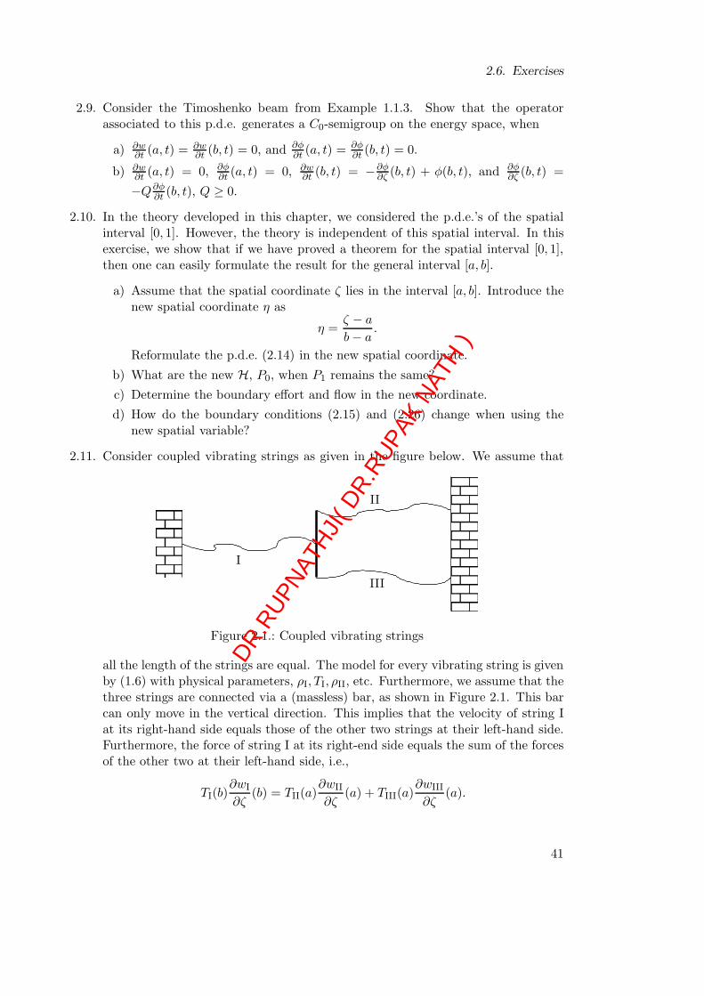
2.6. Exercises

2.9. Consider the Timoshenko beam from Example 1.1.3. Show that the operatorassociated to this p.d.e. generates a C0-semigroup on the energy space, when

a) ∂w∂t (a, t) = ∂w

∂t (b, t) = 0, and ∂φ∂t (a, t) = ∂φ

∂t (b, t) = 0.

b) ∂w∂t (a, t) = 0, ∂φ

∂t (a, t) = 0, ∂w∂t (b, t) = −∂φ

∂ζ (b, t) + φ(b, t), and ∂φ∂ζ (b, t) =

−Q∂φ∂t (b, t), Q ≥ 0.

2.10. In the theory developed in this chapter, we considered the p.d.e.’s of the spatialinterval [0, 1]. However, the theory is independent of this spatial interval. In thisexercise, we show that if we have proved a theorem for the spatial interval [0, 1],then one can easily formulate the result for the general interval [a, b].

a) Assume that the spatial coordinate ζ lies in the interval [a, b]. Introduce thenew spatial coordinate η as

η =ζ − a

b− a.

Reformulate the p.d.e. (2.14) in the new spatial coordinate.

b) What are the new H, P0, when P1 remains the same?

c) Determine the boundary effort and flow in the new coordinate.

d) How do the boundary conditions (2.15) and (2.26) change when using thenew spatial variable?

2.11. Consider coupled vibrating strings as given in the figure below. We assume that

I

II

III

Figure 2.1.: Coupled vibrating strings

all the length of the strings are equal. The model for every vibrating string is givenby (1.6) with physical parameters, ρI, TI, ρII, etc. Furthermore, we assume that thethree strings are connected via a (massless) bar, as shown in Figure 2.1. This barcan only move in the vertical direction. This implies that the velocity of string Iat its right-hand side equals those of the other two strings at their left-hand side.Furthermore, the force of string I at its right-end side equals the sum of the forcesof the other two at their left-hand side, i.e.,

TI(b)∂wI

∂ζ(b) = TII(a)

∂wII

∂ζ(a) + TIII(a)

∂wIII

∂ζ(a).

41

DR.RUPN

ATHJI(

DR.R

UPAK

NATH )

2. Homogeneous differential equation

As depictured, the strings are attached to a wall.

a) Identify the boundary conditions for the system given in Figure 2.1.

b) Formulate the coupled strings as depictured in Figure 2.1 as a Port-Hamiltoniansystem (2.14) and (2.15). Furthermore, determine the energy space X.

c) Show that the differential operator associated to the above system generatesa contraction semigroup on the energy space X.

2.12. Consider transmission lines in a network as depictured in Figure 2.2. In the cou-

VV

II

Trans. line I

Trans. line II

Trans. line III

Trans. line IVKK

Figure 2.2.: Coupled transmission lines

pling parts K, we have that Kirchhoff laws holds. Hence charge flowing out of thetransmission line I, enters II and III, etc. Thus for the coupling between I and IIand III, there holds

VI(b) = VII(a) = VIII(a)

andII(b) = III(a) + IIII(a).

a) Identify the boundary conditions for the system induced by the second cou-pling in Figure 2.2.

b) Formulate the coupled transmission lines as depictured in Figure 2.2 as aPort-Hamiltonian system (2.14). Furthermore, identify the boundary effortand flow, and the energy space X.

c) If the voltage at both ends is set to zero, i.e., VI(a) = 0, VIV(b) = 0, thenshow that the differential operator associated to the above system generatesa contraction semigroup on the energy space X.

d) If left end side is coupled to the right-hand side, i.e., the voltage and currentat both ends are equal, then show that the differential operator associated tothe above system generates a unitary group on the energy space X.

2.7. Notes and references

More on semigroups can be found in [5]. The result of Section 2.3 are taken from [9].

42

DR.RUPN

ATHJI(

DR.R

UPAK

NATH )

Chapter 3

Boundary Control Systems

In this chapter we add a control function to the partial differential equation (1.25), seealso (2.14). In particular, we are interested in boundary controls and we will show thatthese systems have well-defined solutions. We explain our ideas by means of an example,the controlled transport equation, which is given by

∂x

∂t(ζ, t) =

∂x

∂ζ(ζ, t), ζ ∈ [0, 1], t ≥ 0

x(ζ, 0) = x0(ζ), ζ ∈ [0, 1] (3.1)

x(1, t) = u(t), t ≥ 0

for a control function u. In Chapter 2 we have solved the partial differential equationfor the specific choice u = 0. In this chapter we show that the solution of (3.1) is givenby

x(ζ, t) =

x0(ζ + t) ζ + t ≤ 1

u(ζ + t− 1) ζ + t > 1

and that in a similar manner the partial differential equation (1.25) with a boundarycontrol can be treated.

In Section 3.1 we first have to study some abstract theory, which enables us to showthat for certain boundary controls the partial differential equation (1.25) possesses aunique solution.

3.1. Inhomogeneous differential equations

In Chapter 2 we have studied homogeneous (abstract) ordinary differential equations ofthe form

x(t) = Ax(t), x(0) = x0. (3.2)

Under the assumption that A generates a strongly continuous semigroup (T (t))t≥0 weshowed that the solution of (3.2) is given by

x(t) = T (t)x0.

43

DR.RUPN

ATHJI(

DR.R

UPAK

NATH )

3. Boundary Control Systems

In order to be able to add control operators to equation (3.2) we have to study in-homogeneous (abstract) ordinary differential equations first. Such an inhomogeneousequation is given by

x(t) = Ax(t) + f(t), x(0) = x0. (3.3)

We assume that f is a continuous function with values in the Hilbert space X. Later,when we deal with input and control functions f(t) has usually the form Bu(t).

First we have to define what we mean by a solution of (3.3), and we begin with thenotion of a classical solution. The function x(t) is called a classical solution of (3.3)on an interval [0, τ ] if x(t) is a continuous function on [0, τ ] whose derivative is againcontinuous on [0, τ ], x(t) ∈ D(A) for all t ∈ [0, τ ] and x(t) satisfies (3.3) for all t ∈ [0, τ ].

Assume that f ∈ C([0, τ ];X) and that x is a classical solution of (3.3) on [0, τ ]. Thenformally we have

d

ds[T (t− s)x(s)] = T (t− s)x(s) −AT (t− s)x(s)

= T (t− s)[Ax(s) + f(s)] −AT (t− s)x(s)

= T (t− s)f(s),

which implies

∫ t

0T (t− s)f(s) ds =

∫ t

0

d

ds[T (t− s)x(s)] ds = T (t− t)x(t) − T (t− 0)x(0)

= x(t) − T (t)x0.

Equivalently,

x(t) = T (t)x0 +

∫ t

0T (t− s)f(s)ds.

This equation is known as the variation of constant formula. The next lemma showsthat the formal argument which we used to derive this formula can be made precise. Forthe proof we refer to Section 3.5.

Lemma 3.1.1. Assume that f ∈ C([0, τ ];X) and that x is a classical solution of (3.3)on [0, τ ]. Then Ax(·) is an element of C([0, τ ];X), and

x(t) = T (t)x0 +

∫ t

0T (t− s)f(s)ds. (3.4)

This lemma tells us how a classical solution will look like, but does not tells us anythingabout existence and uniqueness of solutions. This is the subject of the following theorem,whose proof is given in Section 3.5

Theorem 3.1.2. If A is the infinitesimal generator of a C0-semigroup (T (t))t≥0 on a

Hilbert space X, f ∈ C1([0, τ ];X) and x0 ∈ D(A), then (3.4) is continuously differen-tiable on [0, τ ] and it is the unique classical solution of (3.3).

44

DR.RUPN

ATHJI(

DR.R

UPAK

NATH )

3.1. Inhomogeneous differential equations

By taking f = 0 and x0 6∈ D(A), it is clear that (3.4) will not be the classical solutionof (3.3) in general. Although (3.4) is only a classical solution for special initial statesx0 and smooth functions f , we see that this equation is well-defined for every t ≥ 0and every x0 ∈ X and f ∈ L2([0, τ ];X). Furthermore, for x1 ∈ D(A∗), one can showthat 〈x1, x(t)〉 is continuous differentiable, and satisfies (3.4) weakly. Therefore, for anyx0 ∈ X and every f ∈ L2([0, τ ];X) we call (3.4) the solution of (3.3). Since we sometimeswant to distinguish between this solution and the classical solution, we use the namemild solution for the variation of constant formula (3.4).

Most times the inhomogeneous differential equation (3.3) is of the form

x(t) = Ax(t) +Bu(t), x(0) = x0, (3.5)

where B is a linear bounded operator from the input space U to the state space X. Thespaces U and X are Hilbert spaces. u is considered as the (control) input and B is thecontrol operator. This is a special case of (3.3) via f(t) = Bu(t). Hence the (mild)solution of (3.5) is given by

x(t) = T (t)x0 +

∫ t

0T (t− s)Bu(s) ds (3.6)

for every x0 ∈ X and every u ∈ L2([0, τ ];X). We apply this to our simple example ofthe transport equation.

Example 3.1.3 We study the following controlled partial differential equation

∂x

∂t(ζ, t) =

∂x

∂ζ(ζ, t) + u(t)

x(1, t) = 0.

We can write this partial differential equation as

x(t) = Ax(t) +Bu(t)

with, see also Examples 2.2.7 and 2.3.3,

Ax =dx

dζ,

D(A) =x ∈ L2(0, 1) | x ∈ H1(0, 1) and x(1) = 0

,

Bu = 1 · u.

In Chapter 2 we have shown that A generates a C0-semigroup on L2(0, 1). Using theformula for the semigroup generated by A, see Examples 2.2.3 and 2.2.5 we get

x(ζ, t) = x0(ζ + t)1[0,1](ζ + t) +

∫ t

01[0,1](ζ + t− τ)u(τ) dτ,

where 1[0,1](ζ) = 1 if ζ ∈ [0, 1] and 1[0,1](ζ) = 0 otherwise.

45

DR.RUPN

ATHJI(

DR.R

UPAK

NATH )

3. Boundary Control Systems

In this example we applied a control within the spatial domain. More logical forthis example is to apply a control at the boundary. However, when doing so, we cannotrewrite this system in our standard form (3.5), see Example 3.2.3. This is general the casewhen controlling a p.d.e. via its boundary. Thus systems with control at the boundaryform a new class of systems, and are introduced next.

3.2. Boundary control systems

We first explain the idea by means of the controlled transport equation (3.1). Considerthe following system

∂x

∂t(ζ, t) =

∂x

∂ζ(ζ, t), ζ ∈ [0, 1], t ≥ 0

x(ζ, 0) = x0(ζ), ζ ∈ [0, 1] (3.7)

x(1, t) = u(t), t ≥ 0.

for an input u ∈ L2(0, τ).Boundary control problems like the one above occur frequently in our applications,

but unfortunately they do not fit into our standard formulation (3.5). However, forsufficiently smooth inputs it is possible to reformulate such problems so that they dolead to an associated system in the standard form (3.5). In order to find the associatedsystem for the controlled transport equation we use the following trick. Assume that x isa classical solution of the p.d.e. (3.7) and that u is continuously differentiable. Defining

v(ζ, t) = x(ζ, t) − u(t),

we obtain the following partial differential equation for v

∂v

∂t(ζ, t) =

∂v

∂ζ(ζ, t) − u(t), ζ ∈ [0, 1], t ≥ 0

v(1, t) = 0, t ≥ 0.

This partial differential equation for v can be written in the standard form as

v(t) = Av(t) +Bu(t)

for u = u. Hence by applying a simple trick, we can reformulate a p.d.e. with boundarycontrol into a p.d.e. with internal control. The price we have to pay is that u has to besmooth.

The trick applied to (3.7) can be extended to abstract boundary control systems:

x(t) = Ax(t), x(0) = x0,

Bx(t) = u(t),(3.8)

where A : D(A) ⊂ X 7→ X, u(t) ∈ U , U is a Hilbert space, and the boundary operatorB : D(B) ⊂ X 7→ U satisfies D(A) ⊂ D(B).

In order to reformulate equation (3.8) into an abstract form (3.5), we need to imposeextra conditions on the system.

46

DR.RUPN

ATHJI(

DR.R

UPAK

NATH )

3.2. Boundary control systems

Definition 3.2.1. The control system (3.8) is a boundary control system if the followinghold:

a. The operator A : D(A) 7→ X with D(A) = D(A) ∩ ker(B) and

Ax = Ax for x ∈ D(A) (3.9)

is the infinitesimal generator of a C0-semigroup on X;

b. There exists a B ∈ L(U,X) such that for all u ∈ U , Bu ∈ D(A), the operator ABis an element of L(U,X) and

BBu = u, u ∈ U. (3.10)

♣

Part b. of the definition is equivalent to the fact that the range of the operator B

equals U . Note that Part a. of the definition guarantees that the system possesses aunique solution for the choice u(t) = 0, i.e., the homogeneous equation is well-posed.Part b. allows us to choose every value in U for u(t). In other words, the values of inputsare not restricted, which is a logical condition for inputs.

We say that the function x(t) is a classical solution of the boundary control systemof Definition 3.2.1 if x(t) is a continuously differentiable function, x(t) ∈ D(A) for all t,and x(t) satisfies (3.8) for all t.

For a boundary control system, we can apply a similar trick as the one applied in thebeginning of this section. This is the subject of the following theorem. It turns out thatv(t) = x(t) −Bu(t) is a solution of the abstract differential equation

v(t) = Av(t) −Bu(t) + ABu(t),

v(0) = v0.(3.11)

Since A is the infinitesimal generator of a C0-semigroup and B and AB are boundedlinear operators, we have from Theorem 3.1.2 that equation (3.11) has a unique classicalsolution for v0 ∈ D(A). Furthermore, we can prove the following relation between the(classical) solutions of (3.8) and (3.11).

Theorem 3.2.2. Consider the boundary control system (3.8) and the abstract Cauchyequation (3.11). Assume that u ∈ C2([0, τ ];U) for all τ > 0. Then, if v0 = x0 −Bu(0) ∈D(A), the classical solutions of (3.8) and (3.11) are related by

v(t) = x(t) −Bu(t). (3.12)

Furthermore, the classical solution of (3.8) is unique.

Proof: Suppose that v(t) is a classical solution of (3.11). Then v(t) ∈ D(A) ⊂ D(A) ⊂D(B), Bu(t) ∈ D(B), and so

Bx(t) = B[v(t) +Bu(t)] = Bv(t) + BBu(t) = u(t),

47

DR.RUPN

ATHJI(

DR.R

UPAK

NATH )

3. Boundary Control Systems

where we have used that v(t) ∈ D(A) ⊂ ker B and equation (3.10). Furthermore, from(3.12) we have

x(t) = v(t) +Bu(t)

= Av(t) −Bu(t) + ABu(t) +Bu(t) by (3.11)

= Av(t) + ABu(t)

= A(v(t) +Bu(t)) by (3.9)

= Ax(t) by (3.12).

Thus, if v(t) is a classical solution of (3.11), then x(t) defined by (3.12) is a classicalsolution of (3.8).

The other implication is proved similarly. The uniqueness of the classical solutions of(3.8) follows from the uniqueness of the classical solutions of (3.11).

The (mild) solution of (3.11) is given by

v(t) = T (t)v(0) +

∫ t

0T (t− τ)[ABu(τ) −Bu(τ)] dτ (3.13)

for every v(0) ∈ X and every u ∈ H1(0,∞);U). Therefore, the function

x(t) = T (t)(x0 −Bu(0)) +

∫ t

0T (t− τ)[ABu(τ) −Bu(τ)] dτ +Bu(t) (3.14)

is called the mild solution of the abstract boundary control system (3.8) for every x0 ∈ Xand every u ∈ H1((0,∞);U).

As an example we study again the controlled transport equation from the beginningof this section.

Example 3.2.3 We consider the following system

∂x

∂t(ζ, t) =

∂x

∂ζ(ζ, t), ζ ∈ [0, 1], t ≥ 0

x(ζ, 0) = x0(ζ), ζ ∈ [0, 1]

x(1, t) = u(t), t ≥ 0.

for an input u ∈ H1(0, τ). In order to write this example in the form (3.8) we chooseX = L2(0, 1) and

Ax =dx

dζ, D(A) =

x ∈ L2(0, 1) | x ∈ H1(0, 1)

,

Bx = x(1), D(B) = D(A).

These two operators satisfy the assumption of a boundary control system. More pre-cisely: the operators A and B are linear, A restricted to the domain D(A) ∩ ker B

generates a C0-semigroup, see Example 2.2.7. Furthermore, the range of B is C = U

48

DR.RUPN

ATHJI(

DR.R

UPAK

NATH )

3.2. Boundary control systems

and the choice B = 1 implies BBu = u. Using AB = 0, we conclude from equation(3.14) that the solution is given by

x(t) = v(t) +Bu(t)

= T (t)v(0) +

∫ t

0T (t− τ)[ABu(τ) −Bu(τ)] dτ +Bu(t)

= T (t)v(0) −∫ t

0T (t− τ)u(τ) dτ + u(t).

Using the precise form of the shift-semigroup, see Example 2.2.3, we can write thesolution of the boundary controlled partial differential equation as

x(ζ, t) = v0(ζ + t)1[0,1](ζ + t) −∫ t

01[0,1](ζ + t− τ)u(τ) dτ + u(t).

If ζ + t > 1, we have

x(ζ, t) = −[u(τ)]|tζ+t−1 + u(t) = u(ζ + t− 1),

and if ζ + t ≤ 1, then

x(ζ, t) = v0(ζ + t) − [u(τ)]|t0 + u(t) = v0(ζ + t) + u(0) = x0(ζ + t).

Or equivalently,

x(ζ, t) =

x0(ζ + t) ζ + t ≤ 1

u(ζ + t− 1) ζ + t > 1(3.15)

which proves our claim made on the first page of this chapter.

Now it is not hard to show that the controlled p.d.e. form this example cannot bewritten as the abstract control system

x(t) = Ax(t) +Bu(t), (3.16)

with B a bounded operator. Since for u = 0, we have that the p.d.e. becomes thehomogeneous equation of Examples 2.2.5 and 2.2.7, we have that A can only be A

restricted to D(A) ∩ ker B. Hence the semigroup is the shift semigroup.

If our controlled p.d.e. would be of the form (3.16), then by Theorem 3.1.2, we wouldhave that x(t) ∈ D(A), whenever x0 ∈ D(A) and f ∈ C1((0, τ ;X). Choosing x0 ∈ D(A)and u = 1, we see by (3.15), that x(1, t) = u(t). Since this is unequal to zero, wehave that x(t) 6∈ D(A). Concluding we find that the boundary controlled p.d e. of thisexample cannot be written in the form (3.16).

The controlled transport equation is a simple example of our general class of port-Hamiltonian systems. This example could be written as a boundary control system. Inthe following section, we show that this holds in general for a port-Hamiltonian system.

49

DR.RUPN

ATHJI(

DR.R

UPAK

NATH )

3. Boundary Control Systems

3.3. Port-Hamiltonian systems as boundary control systems

In this section we add a boundary control to our Hamiltonian system and we showthat the assumptions of a boundary control system are satisfied. The port-Hamiltoniansystem with control is given by

∂x

∂t(ζ, t) = P1

∂

∂ζ[Hx(t)] + P0[Hx(t)] (3.17)

u(t) = WB,1

(f∂(t)e∂(t)

)(3.18)

0 = WB,2

(f∂(t)e∂(t)

). (3.19)

We first recall the defining operators of the port-Hamiltonian system. As in Section 2.3we assume that

• P1 is an invertible, symmetric real n× n-matrix;

• P0 is an anti-symmetric real n× n-matrix;

• H(ζ) is a symmetric, invertible n× n-matrix for every ζ ∈ [a, b] and mI ≤ H(ζ) ≤MI for some m,M > 0 independent of ζ;

• WB :=(WB,1

WB,2

)is a full rank real matrix of size n× 2n.

We recall that the boundary effort and flow are given by, see (2.24)

(f∂(t)e∂(t)

)= R0

(H(b)x(b, t)H(a)x(a, t)

)

where R0 is the invertible n× n-matrix defined in (2.21).

We can write the Hamiltonian system as a boundary control system

x(t) = Ax(t), x(0) = x0,

Bx(t) = u(t),

by defining

Ax = P1∂

∂ζ[Hx] + P0[Hx], (3.20)

D(A) =

x ∈ L2((a, b); Rn) | Hx ∈ H1((a, b); Rn),WB,2

(f∂e∂

)= 0

, (3.21)

Bx = WB,1

(f∂e∂

), (3.22)

D(B) = D(A). (3.23)

50

DR.RUPN

ATHJI(

DR.R

UPAK

NATH )

3.3. Port-Hamiltonian systems as boundary control systems

As in Section 2.3 we have chosen the Hilbert space X = L2((a, b); Rn) equipped withthe inner product

〈f, g〉X :=1

2

∫ b

af(ζ)TH(ζ)g(ζ) dζ

as our state space. The input space U equals Rk, where k is the number of rows of WB,1.We are now in a position to show that the controlled port-Hamiltonian system is indeeda boundary control system.

Theorem 3.3.1. If (WB,1

WB,2

)(0 II 0

)(W TB,1 W T

B,2

)≥ 0, (3.24)

then the system (3.17)–(3.19) is a boundary control system on X. Furthermore, theoperator

Ax = P1∂

∂ζ[Hx] + P0[Hx] (3.25)

with the domain

D(A) =

Hx ∈ H1((a, b); Rn |

(f∂e∂

)∈ ker

(WB,1

WB,2

)(3.26)

generates a contraction semigroup on X.

Proof: We begin with the simple observation that

(f∂e∂

)∈ ker

(WB,1

WB,2

)

is equivalent to

WB

(f∂e∂

)=

(WB,1

WB,2

)(f∂e∂

)= 0.

From Theorem 2.3.2 follows that the operator A defined in (3.25) and (3.26) is theinfinitesimal generator of a contraction semigroup on X. Moreover, by (3.21) and (3.22)we have that D(A) = D(A) ∩ ker B. Hence part a. of Definition 3.2.1 is satisfied.

The n × 2n-matrix WB is of full rank n and R0 is an invertible matrix. Thus thereexists a 2n× n-matrix S such that

WBR0S =

(WB,1

WB,2

)R0S =

(Ik 00 0

), (3.27)

where Ik is the identity matrix on Rk. We write S =(S11 S12S21 S22

)and we define the

operator B ∈ L(U,X) by

(Bu)(ζ) := H(ζ)−1

(S11

ζ − a

b− a+ S21

b− ζ

b− a

)u.

51

DR.RUPN

ATHJI(

DR.R

UPAK

NATH )

3. Boundary Control Systems

The definition of B implies that Bu is a square integrable function and that Hx ∈H1((a, b); Rn). Furthermore, from (3.27) it follows that WB,2R0

(S11S21

)= 0. Combining

this with the definition of the boundary effort and flow, we obtain that Bu ∈ D(A).Furthermore, B and AB are linear bounded operators from U to X and using (3.27)once more we see that

BBu = WB,1R0

(S1

S2

)u = u.

Thus the Hamiltonian system is indeed a boundary control system.

As an example we once more study the controlled transport equation.

Example 3.3.2 We consider the system

∂x

∂t(ζ, t) =

∂x

∂ζ(ζ, t), ζ ∈ [0, 1], t ≥ 0 (3.28)

x(ζ, 0) = x0(ζ), ζ ∈ [0, 1].

This system can be written in form (3.17) by choosing n = 1, P0 = 0, P1 = 1 and H = 1.Therefore, we have

R0 =1√2

(1 −11 1

)and

(f∂(t)e∂(t)

)=

1√2

(x(1, t) − x(0, t)x(1, t) + x(0, t)

).

Since n = 1, we can either apply one control or no control at all. The control free casehas been treated in Chapter 2, and so we choose one control. By using the boundaryvariables, the control is written as, see (3.18)

u(t) =(a b

) 1√2

(x(1, t) − x(0, t)x(1, t) + x(0, t)

)=

1√2

[(a+ b)x(1, t) + (b− a)x(0, t)] . (3.29)

Note that WB = (a, b) has full rank if and only if a2 + b2 6= 0.By Theorem 3.3.1 gives that the p.d.e. (3.28) together with (3.29) is a boundary

control system if a2 + b2 6= 0 and 2ab ≥ 0, see (3.24). Thus possible boundary controlsare for example

u(t) = x(1, t), (a = b =

√2

2),

u(t) = 3x(1, t) − x(0, t), (a =√

2, b = 2√

2).

For the control u(t) = −x(1, t) + 3x(0, t) we don’t know the answer.

3.4. Outputs

In the previous sections we have added a control function to our systems. In this sectionadditionally an output is added. We follow the line laid out in the previous sections. We

52

DR.RUPN

ATHJI(

DR.R

UPAK

NATH )

3.4. Outputs

start by assuming that the output equation can be represented via a bounded operator.Since this is normally not the case for observations at the boundary, we have to considerboundary observation separately. For this we directly formulate the result for our port-Hamiltonian systems.

We start with the control system 3.5 to which we add a output equation.

x(t) = Ax(t) +Bu(t), x(0) = x0, (3.30)

y(t) = Cx(t) +Du(t), (3.31)

where B is a linear bounded operator from the input space U to the state space X, Cis a linear bounded operator from X to the output space Y , and D is a linear operatorfrom U to Y . All Spaces U , X and Y are Hilbert spaces.

In Section 3.1 we showed that the solution of (3.30) is given by

x(t) = T (t)x0 +

∫ t

0T (t− s)Bu(s) ds.

This function is well-defined for every x0 ∈ X and every u ∈ L2([0, τ ];U). The outputequation (3.31) only contains bounded operators. Hence there is no difficulty in “solving”this equation. We summarize the answer in the following theorem

Theorem 3.4.1. Consider the abstract equation (3.30)–(3.31), with A the infinitesimalgenerator of the C0-semigroup (T (t))t≥0, and B,C, and D bounded.

The solution of (3.30)–(3.31) is given by the variation of constant formula (3.6)

x(t) = T (t)x0 +

∫ t

0T (t− s)Bu(s) ds,

y(t) = CT (t)x0 + C

∫ t

0T (t− s)Bu(s) ds+Du(t)

for every x0 ∈ X and every u ∈ L2([0, τ ];U).

As said in the beginning of this section, our main focus lies on boundary observa-tion for port-Hamiltonian systems. We develop conditions on the boundary observationguaranteeing that a certain balance equation is satisfied, which are important for Chap-ter 4 and 5. The standard Hamiltonian system with boundary control and boundaryobservation is given by

x(t) = P1∂

∂ζ[Hx(t)] + P0[Hx(t)] (3.32)

u(t) = WB

(f∂(t)e∂(t)

)(3.33)

y(t) = WC

(f∂(t)e∂(t)

). (3.34)

It is assumed that (3.32)–(3.33) satisfy the assumption of a port-Hamiltonian system, seeSection 3.3. Further we assume that WBΣW T

B ≥ 0, where Σ =(

0 II 0

). This guarantees

53

DR.RUPN

ATHJI(

DR.R

UPAK

NATH )

3. Boundary Control Systems

that (3.32)–(3.33) is a boundary control system, see Theorem 3.3.1. Note that we havetaken WB = WB,1 or equivalently WB,2 = 0. In other words, we are using the maximalnumber of control.

The output equation is formulated very similar to the input equation. As for the inputwe assume that we use full measurements, i.e., WC be a full rank matrix of size n× 2n.Since we do not want to measure quantities that we already have chosen as inputs, see

(3.33), we assume that(WB

WC

)is of full rank, or equivalently this matrix is invertible.

Combining this assumption with the fact that Σ is invertible, we see that the product(WB

WC

)Σ (WT

B WTC ) is invertible as well. Its inverse is defined as

PWB,WC=

((WB

WC

)Σ(W TB W T

C

))−1

=

(WBΣW T

B WBΣW TC

WCΣW TB WCΣW T

C

)−1

. (3.35)

Theorem 3.4.2. Consider the system (3.32)–(3.34) with WB a full rank n× 2n matrix

satisfying WBΣW TB ≥ 0, and WC a full rank n×2n matrix such that

(WB

WC

)is invertible.

For every u ∈ C2(0,∞; Rn), Hx(0) ∈ H1((a, b); Rn), and u(0) = WB

(f∂(0)e∂(0)

), the

system (3.32)–(3.34) has a unique (classical) solution, with Hx(t) ∈ H1((a, b); Rn). Theoutput y(·) is continuous, and the following balance equation is satisfied:

d

dt‖x(t)‖2

X =1

2

(uT (t) yT (t)

)PWB,WC

(u(t)y(t)

). (3.36)

Proof: See Exercise 3.1.

As an example we return to the controlled transport equation of Example 3.3.2.

Example 3.4.3 We consider the system

∂x

∂t(ζ, t) =

∂x

∂ζ(ζ, t), ζ ∈ [0, 1], t ≥ 0 (3.37)

x(ζ, 0) = x0(ζ), ζ ∈ [0, 1]

u(t) = x(1, t), t ≥ 0.

In Example 3.3.2 we have already seen that this system can be written in form (3.32)–(3.33) by choosing n = 1, P0 = 0, P1 = 1, H = 1 and WB = (

√2

2

√2

2).

Now we add the output equation

y(t) =(c d

) 1√2

(x(1, t) − x(0, t)x(1, t) + x(0, t)

)=

1√2(c+ d)x(1, t) + (c− d)x(0, t)). (3.38)

Since WC = (c d ) must have full rank, we find that c2 + d2 6= 0. Furthermore, since(WB

WC

)must be invertible, we find that c 6= d.

Hence all conditions of Theorem 3.4.2 are satisfying for this system whenever c 6= d.

For the particular choice c = −d =√

22 , that is y(t) = x(0, t), we find PWB ,WC

=(1 00 −1

), or equivalently

d

dt‖x(t)‖2

X =1

2

(|u(t)|2 − |y(t)|2

).

54

DR.RUPN

ATHJI(

DR.R

UPAK

NATH )

3.5. Some proofs

3.5. Some proofs

This section contains the proofs of Lemma 3.1.1 and Theorem 3.1.2.

Proof: (of Lemma 3.1.1) From (3.3), we have that Ax(t) = x(t) − f(t) and x ∈C([0, τ ];X) shows that Ax(·) ∈ C([0, τ ];X).

We now prove (3.4). Let t be an arbitrary, but fixed, element of (0, τ ] and considerthe function T (t− s)x(s) for s ∈ [0, t). We shall show that this function is differentiablein s. Let h be sufficiently small and consider

T (t− s− h)x(s + h) − T (t− s)x(s)

h

=T (t− s− h)x(s + h) − T (t− s− h)x(s)

h+

T (t− s− h)x(s) − T (t− s)x(s)

h.

If h converges to zero, then the last term converges to −AT (t−s)x(s), since x(s) ∈ D(A).Thus it remains to show that the first term converges. We have the following equality

T (t− s− h)x(s + h) − T (t− s− h)x(s)

h− T (t− s)x(s)

= T (t− s− h)x(s+ h) − x(s)

h− T (t− s− h)x(s) +

T (t− s− h)x(s) − T (t− s)x(s).

The uniform boundedness of T (t) on any compact interval and the strong continuityallow us to conclude from the last equality that

limh→0

‖T (t− s− h)x(s + h) − x(s)

h− T (t− s)x(s)‖ = 0.

So we have proved that

d

ds[T (t− s)x(s)] = T (t− s)x(s) −AT (t− s)x(s)

= T (t− s)[Ax(s) + f(s)] −AT (t− s)x(s)

= T (t− s)f(s).

This implies

∫ t

0T (t− s)f(s) ds =

∫ t

0

d

ds[T (t− s)x(s)] ds = T (t− t)x(t) − T (t− 0)x(0)

= x(t) − T (t)x0.

Thus a classical solution to (3.3) necessarily has the form (3.4).

55

DR.RUPN

ATHJI(

DR.R

UPAK

NATH )

3. Boundary Control Systems

Proof: (of Theorem 3.1.2) Uniqueness: If z1 and z2 are two different solutions, thentheir difference ∆(t) = z1(t) − z2(t) satisfies the differential equation

d∆

dt= A∆, ∆(0) = 0

and so we need to show that its only solution is ∆(t) ≡ 0. To do this, define y(s) =

T (t − s)∆(s) for a fixed t and 0 ≤ s ≤ t. Clearly,dy

ds= 0 and so y(s) = constant

= T (t)∆(0) = 0. However, y(t) = ∆(t) shows that ∆(t) = 0.

Existence: Clearly, all we need to show now is that v(t) =∫ t0 T (t−s)f(s)ds is an element

of C1([0, τ ];X) ∩D(A) and satisfies differential equation (3.3). Now

v(t) =

∫ t

0T (t− s)[f(0) +

∫ s

0f(α)dα]ds

=

∫ t

0T (t− s)f(0)ds+

∫ t

0

∫ t

αT (t− s)f(α)dsdα,

where we have used Fubini’s Theorem A.5.22. From Theorem 2.5.2.e, it follows that

T (t− α)z − z = A

∫ t

αT (t− s)zds for all z ∈ Z.

Hence v(t) ∈ D(A), and∫ t0 ‖A

∫ tα T (t−s)f(α)ds‖dα =

∫ t0 ‖T (t−α)f (α)− f(α)‖dα <∞.

Thus, since A is closed, by Theorem A.5.23 we have that

Av(t) = [T (t) − I]f(0) +

∫ t

0[T (t− α) − I]f(α)dα

= T (t)f(0) +

∫ t

0T (t− α)f(α)dα − f(t).

Now, since the convolution product is commutative, i.e.,∫ t0 g(t−s)h(s)ds =

∫ t0 g(s)h(t−

s)ds, we have that

v(t) =

∫ t

0T (s)f(t− s)ds

and so

dv

dt(t) = T (t)f(0) +

∫ t

0T (s)f(t− s)ds

= T (t)f(0) +

∫ t

0T (t− s)f(s)ds,

once again using commutativity of the convolution product. It follows that dvdt is contin-

uous anddv

dt(t) = Av(t) + f(t).

56

DR.RUPN

ATHJI(

DR.R

UPAK

NATH )

3.6. Exercises

3.6. Exercises

3.1. Prove Theorem 3.4.2. Hint: Use the calculations of the proof of Theorem 2.3.2.

3.2. Consider the transmission line of Example 1.1.1 for any of the following boundarycondition:

a) At the left-end the voltage equal u1(t) and at the right-end the voltage equalsthe input u2(t).

b) At the left-end we put the voltage equal to zero and at the right-end thevoltage equals the input u(t).

c) At the left-end we put the voltage equal to u(t) and at the right-end thevoltage equals R times the current, for some R > 0.

Show that these systems can be written as a boundary control system.

3.3. Consider the vibrating string of Example 1.1.2 with the boundary conditions

∂x

∂ζ(0, t) = 0 and

∂x

∂ζ(1, t) = u(t) t ≥ 0.

Reformulate this system as a boundary control system.

3.4. Consider the Timonshenko beam from Example 1.1.3 for any of the followingboundary condition:

a) ∂w∂t (a, t) = u1(t),

∂w∂t (b, t) = u2(t), and ∂φ

∂t (a, t) = ∂φ∂t (b, t) = 0.

b) ∂w∂t (a, t) = u(t), ∂φ

∂t (a, t) = 0, ∂w∂t (b, t) = −∂φ

∂ζ (b, t) + φ(b, t), and ∂φ∂ζ (b, t) =

−Q∂φ∂t (b, t), Q ≥ 0.

Reformulate these systems as boundary control systems.

3.5. We consider again the transmission line of Exercise 3.2 with boundary conditionsa). Define an output to the system such that

d

dt‖x(t)‖2

X = u(t)T y(t).

3.6. In the formulation of port-Hamiltonian systems as boundary control systems, wehave the possibility that some boundary conditions are set to zero, see (3.19).However, when we add an output, this possibility was excluded, see (3.32)–(3.34).Furthermore, we assumed that we had n outputs. In this exercise we show thatthis did not pose a restriction to the theory.

a) Show that if WB,2 = 0, i.e., WB = WB,1, and WBΣW TB ≥ 0, then (3.17) with

control (3.18) is a well-defined boundary control system. Given the expressionfor the domain of the infinitesimal generator A.

57

DR.RUPN

ATHJI(

DR.R

UPAK

NATH )

3. Boundary Control Systems

b) LetWB be a n×2nmatrix of full rank satisfyingWBΣW TB ≥ 0. We decompose

u = WB

(f∂e∂

)as

u =

(u1

u2

)=

(WB,1

WB,2

)(f∂e∂

).

By using the previous item, show that putting u2 = 0 is allowed. Furthermore,show that it leads to the same boundary control system as in (3.17)–(3.19).

Consider the following system

∂x

∂t(ζ, t) = P1

∂

∂ζ[Hx(t)] + P0[Hx(t)]

u(t) = WB,1

(f∂(t)e∂(t)

)

0 = WB,2

(f∂(t)e∂(t)

)

y(t) = WC

(f∂(t)e∂(t)

)

where we assume that WB =(WB,1

WB,2

)is a full rank matrix of size n× 2n satisfying

WBΣW TB ≥ 0. Furthermore, WC is a full-rank matrix of size k × 2n satisfying

rank

(WB

WC

)= n+ k.

c) Explain why the above rank conditions are logical.

d) Show that the above system is well-defined. In particular show that forsmooth inputs and initial conditions, we have a unique solution, with thestate and output trajectory continuous.

3.7. Consider the vibrating string of Exercise 3.3 with the boundary conditions

∂x

∂ζ(0, t) = 0 and

∂x

∂ζ(1, t) = u(t) t ≥ 0.

and we measure the velocity at ζ = 0.

a) Prove that this is a well-defined input-output system.

Hint: Use the previous exercise.

b) Does a balance equation like (3.36) hold?

c) Repeat the above two questions for the measurement y(t) = ∂w∂t (1, t).

3.8. Consider the coupled strings of Exercise 2.11. Now we apply a force u(t), to thebar in the middle, see Figure 3.1. This implies that the force balance in the middlebecomes

TI(b)∂wI

∂ζ(b) = TII(a)

∂wII

∂ζ(a) + TIII(a)

∂wIII

∂ζ(a) + u(t).

58

DR.RUPN

ATHJI(

DR.R

UPAK

NATH )

3.6. Exercises

I

II

III

u(t)

Figure 3.1.: Coupled vibrating strings with external force

a) Formulate the coupled vibrating strings with external force as a boundarycontrol system.

b) Additionally, we measure the velocity of the bar in the middle. Reformatethe system with this output as (3.32)–(3.34).

c) For the input and output defined above, determine the power balance in termsof the input and output, see (3.36).

59

DR.RUPN

ATHJI(

DR.R

UPAK

NATH )

3. Boundary Control Systems

60

DR.RUPN

ATHJI(

DR.R

UPAK

NATH )

Chapter 4

Transfer Functions

In this chapter we discuss the concept of transfer functions. Let us first recapitulate theconcept for finite-dimensional systems. Consider the ordinary differential equation

y(t) + 3y(t) − 7y(t) = −u(t) + 2u(t), (4.1)

where the dot denotes the derivative with respect to time. In many textbooks one derivesthe transfer function by taking the Laplace transform of this differential equation underthe assumption that the initial conditions are zero. Since the following rules hold for theLaplace transform

f(t) → F (s) − f(0)

f(t) → s2F (s) − sf(0) − f(0),

we have that after Laplace transformation the differential equation becomes the algebraicequation:

s2Y (s) + 3sY (s) − 7Y (s) = −sU(s) + 2U(s). (4.2)

This implies that

Y (s) =−s+ 2

s2 + 3s− 7U(s). (4.3)

The rational function in front of U(s) is called the transfer function associated with thedifferential equation (4.1).

This is a standard technique, but there are some difficulties with it if we want to extendit to partial differential equations. One of the difficulties is that one has to assume that uand y are Laplace transformable. Since u is chosen, this is not a strong assumption, butonce u is chosen, y is dictated by the differential equation, and it is not known a priorywhether it is Laplace transformable. Furthermore, the Laplace transform only existsin some right half-plane of the complex plane. This implies that we have the equality(4.3) for those s in the right-half plane for which the Laplace transform of u and y bothexist. The right-half plane in which the Laplace transform exists is named the region ofconvergence. Even for the simple differential equation (4.1) equality (4.3) does not hold

61

DR.RUPN

ATHJI(

DR.R

UPAK

NATH )

4. Transfer Functions

everywhere. Taking into account the region of convergence of both u and y, we find that(4.3) only holds for those s which lies right of the poles, i.e., the zeros of s2 + 3s − 7.

To overcome all these difficulties we define the transfer function in a different way.We shall look for solutions of the differential equation which are exponentials. Let usillustrate this for the simple differential equation of (4.1). Given s ∈ C, we look for asolution pair of the form (u(t), y(t)) = (est, yse

st). If for an s such a solution exists, andit is unique, then we call ys the transfer function of (4.1) in the point s. Substitutingthis pair into our differential equation, we have

s2ysest + 3syse

st − ysest = −sest + 2est. (4.4)

We recognize the common term est which is never zero, and so we may divide by it.After this division, we obtain

s2ys + 3sys − ys = −s+ 2. (4.5)

This is uniquely solvable for ys if and only if s2 + 3s− 7 6= 0.

We see that we have obtained, without running into mathematical difficulties, thetransfer function. Since for p.d.e.’s or for abstract differential equations the concept ofa solution is well-defined, we may define transfer function via exponential functions.

4.1. Basic definition and properties

In this section we start with a very general definition of a transfer function, which evenapplies to systems not described by a p.d.e, but via e.g. a difference differential equationor an integral equation. To formulate this definition, we first have to introduce a generalsystem. In a general system, we have a time axis, T, which is assumed to be a subset ofR. Furthermore, we distinguish three spaces, U , Y , and R. U and Y are the input- andoutput space, respectively, whereas R contains the rest of the variables. In our examples,R will become the state space. A system S is a subset of (U ×R× Y )T, i.e., a subsetof all functions from T to U ×R× Y .

Definition 4.1.1. Let S be a system, let s be an element of C, and let u0 ∈ U . We saythat (u0e

st, r(t), y(t)) is an exponential solution in S if there exist r0 ∈ R, y0 ∈ Y , suchthat (u0e

st, r0est, y0e

st) = (u0est, r(t), y(t)), t ∈ T.

If for every u0 ∈ U the output trajectory, y0est, corresponding to an exponential

solution is unique, then we call the mapping u0 7→ y0 the transfer function at s. Wedenote this mapping by G(s). Let Ω ⊂ C be the set consisting of all s for which thetransfer function at s exists. The mapping s ∈ Ω 7→ G(s) is defined as the transferfunction of the system S. ♣

Recall that a system is said to be linear if U , R, and Y are linear spaces, and if(αu1 + βu2, αr1 + βr2, αy1 + βy2) ∈ S whenever (u1, r1, y1) and (u2, r2, y2) are in S.The system is time-invariant , when T is an interval of the form (t0,∞), t0 ≥ −∞, and(u(· + τ), r(· + τ), y(· + τ)) is in S for all τ > 0, whenever (u, r, y) ∈ S.

62

DR.RUPN

ATHJI(

DR.R

UPAK

NATH )

4.1. Basic definition and properties

Lemma 4.1.2. Consider the abstract system S which is linear and time-invariant onthe time axis [0,∞). If S is such that (0, 0, y(t)) ∈ S implies that y(t) is the zerofunction, then exponential u and r implies exponential y, i.e., if (u0e

st, r0est, y(t)) ∈ S,

then y(t) = y0est for some y0 ∈ Y .

Additionally, assume that for a given s ∈ C there exists an exponential solution forall u0 ∈ U , and assume that (0, r0e

st, y(t)) ∈ S implies that r0 = 0. Then the transferfunction at s exists, and is a linear mapping.

Proof: Let (u0estr0e

st, y(t)) be an element of S, and let τ ≥ 0. Combining the linearityand time-invariance, we see that

(0, 0, y(t + τ) − esτy(t)) = (u0es(t+τ), r0e

s(t+τ), y(t+ τ)) − (u0esτest, r0e

sτest, esτy(t))

is an element of S. By assumption, this implies that y(t+τ) = esτy(t) for all τ . Choosingt = 0, gives the desired result.

Now assume that for a given s ∈ C there exists an exponential solution for all u0 ∈ U .First we show that the exponential solution is unique. When (u0e

st, r0est, y0e

st) and(u0e

st, r0est, y0e

st) are both in S, then by the linearity (0, (r0 − r0)est, (y0 − y0)e

st) ∈ S.By our assumption this implies that r0 = r0 and y0 = y0.

From this we see that we can define a mapping u0 7→ y0. It remains to show that thismapping is linear. Let (u10e

st, r10est, y10e

st) and (u20est, r20e

st, y20est) be two exponen-

tial solutions. By the linearity, it is easy to see that

((αu10 + βu20)est, (αr10 + βr20)e

st, (αy10 + βy20)est) ∈ S

Hence this implies that αu10 + βu20 is mapped to αy10 + βy20. In other words, themapping is linear.

In our applications r will be the state x. It turns out that for the class of systemswe are considering, the conditions in the above lemma are very weak, see Exercise 4.1.Thus the transfer function exists, and is a linear operator.

We begin by showing that the transfer function for the system

x(t) = Ax(t) +Bu(t) (4.6)

y(t) = Cx(t) +Du(t), (4.7)

where B, C and D are bounded operators and A generates a strongly continuous semi-group, is given by the familiar formula G(s) = C(sI −A)−1B+D, for s in the resolventset, ρ(A), of A.

Theorem 4.1.3. Consider the state linear system (4.6)–(4.7), withB, C, andD boundedoperators. As solutions of this system we take the mild solutions, see Theorem 3.4.1.

If (u(t), x(t), y(t)) is an exponential solution, then it is a classical solution as well.Furthermore, for s ∈ ρ(A), the transfer function exists and is given by

G(s) = C(sI −A)−1B +D. (4.8)

63

DR.RUPN

ATHJI(

DR.R

UPAK

NATH )

4. Transfer Functions

Proof: The mild solution of (4.6) is given by

x(t) = T (t)x0 +

∫ t

0T (t− τ)Bu(τ)dτ (4.9)

For an exponential solution this becomes

x0est = T (t)x0 +

∫ t

0T (t− τ)Bu0e

sτdτ. (4.10)

By taking Laplace transforms, this equality becomes

x0

λ− s= (λI −A)−1x0 + (λI −A)−1Bu0

1

λ− s(4.11)

for λ ∈ C with Re(λ) > maxRe(s), ω0, where ω0 is the growth bound of (T (t))t≥0.Since for fixed λ the right-hand side of (4.11) is an element of D(A), the same holds

for the left-hand side. In other words, x0 ∈ D(A). By Theorem 3.1.2, we conclude thatx(t) is a classical solution.

Equation (4.11) can be rewritten as

x0 − (λ− s)(λI −A)−1x0 = (λI −A)−1Bu0. (4.12)

Multiplying this by (λI −A), we obtain (sI −A)x0 = Bu0. Thus for s ∈ ρ(A),

x0 = (sI −A)−1Bu0. (4.13)

Using the output equation of our system, we have that

y0est = y(t) = Cx(t) +Du(t) = Cx0e

st +Du0est = C(sI −A)−1Bu0e

st +Du0est.

Hence y0 = C(sI −A)−1Bu0 +Du0 which proves (4.8).

The above theorem shows that for state-space systems of the form (4.6)–(4.7) thetransfer function exists, and is given by the formula well-known from finite-dimensionalsystem theory. Our main class of systems, the port-Hamiltonian systems have theircontrol and observation at the boundary, and are not of the form (4.6)–(4.7). As provedin Theorem 3.3.1, they form a subclass of the boundary control systems. In the follow-ing theorem, we formulate transfer functions for boundary control systems. As in theprevious theorem, exponential solutions are always classical solutions.

Theorem 4.1.4. Consider the system

x(t) = Ax(t), x(0) = x0

u(t) = Bx(t) (4.14)

y(t) = Cx(t)

where (A,B) satisfies the conditions for boundary control system, see Definition 3.2.1and C is a bounded linear operator from D(A) to Y , with Y a Hilbert space.

64

DR.RUPN

ATHJI(

DR.R

UPAK

NATH )

4.1. Basic definition and properties

As the class of solutions we take the mild solutions, see equation (3.14).If (u(t), x(t), y(t)) is an exponential solution, then it is a classical solution as well.

Furthermore, for s ∈ ρ(A), the transfer function exists and is given by

G(s) = C(sI −A)−1 [AB − sB] + CB (4.15)

for s ∈ ρ(A).For s ∈ ρ(A) and u0 ∈ U , G(s) can also be found as the (unique) solution of

sx0 = Ax0

u0 = Bx0 (4.16)

G(s)u0 = Cx0,

with x0 ∈ D(A).

Proof: The proof is very similar to that of Theorem 4.1.3. By (3.14) we know that themild solution is given by

x(t) = T (t)(x0 −Bu(0)) +

∫ t

0T (t− τ) [ABu(τ) −Bu(τ)] dτ +Bu(t).

Assuming that (u(t), x(t), y(t)) is an exponential solution, the above equation becomes

estx0 = T (t)(x0 −Bu0) +

∫ t

0T (t− τ) [ABesτu0 −Bsesτu0] dτ +Bestu0.

Taking Laplace transforms, we find for λ ∈ C with Re(λ) > maxRe(s), ω0, where ω0

is the growth bound of the semigroup (T (t))t≥0,

x0

λ− s= (λI −A)−1(x0 −Bu0) + (λI −A)−1

[AB

u0

λ− s−B

su0

λ− s

]+B

u0

λ− s.

Or equivalently,

x0 −Bu0

λ− s= (λI −A)−1(x0 −Bu0) + (λI −A)−1

[AB

u0

λ− s−B

su0

λ− s

].

This implies that x0 −Bu0 ∈ D(A), and

(λI −A)[x0 −Bu0] = [x0 −Bu0](λ− s) + ABu0 −Bsu0.

Subtracting the term λ[x0 −Bu0] from both sides, this becomes

(sI −A)[x0 −Bu0] = ABu0 −Bsu0. (4.17)

For s ∈ ρ(A), this gives

x0 = (sI −A)−1 [AB − sB]u0 +Bu0. (4.18)

65

DR.RUPN

ATHJI(

DR.R

UPAK

NATH )

4. Transfer Functions

Since x0 −Bu0 ∈ D(A) and since u ∈ C2([0,∞);U) we have by Theorem 3.2.2 that x(t)is a classical solution of (4.14). In particular, for all t ≥ 0, x(t) ∈ D(A). By assumptionthe domain of C contains the domain of A. Hence y0e

st = y(t) = Cx(t), holds point-wisein t. Taking t = 0, gives y0 = Cx0. Combining this equality with (4.18), we obtain(4.15).

Since x(t) = x0est is a classical solution for u(t) = u0e

st, we can substitute this in thedifferential equation (4.14). By doing so we find

sx0est = Ax0e

st

u0est = Bx0e

st

y0est = Cx0e

st

Removing the exponential term, we find equation (4.16). The uniqueness of x0 followsby (4.18).

We close this section by calculating the transfer function for the simple Example 3.4.3.

Example 4.1.5 Consider the system

∂x

∂t(ζ, t) =

∂x

∂ζ(ζ, t), ζ ∈ [0, 1], t ≥ 0 (4.19)

x(ζ, 0) = x0(ζ), ζ ∈ [0, 1]

u(t) = x(1, t), t ≥ 0.

y(t) = x(0, t), t ≥ 0.

If we define Cx = x(0), then it is easy to see that all assumptions in Theorem 4.1.4 aresatisfied, see Theorem 3.3.1. Hence we can calculate the transfer function, we do thisvia the equation (4.16). For the system (4.19) this becomes

sx0(ζ) =∂x0

∂ζ(ζ) =

dx0

dζ(ζ)

u0 = x0(1)

G(s)u0 = x0(0).

The above differential equation has the solution x0(ζ) = αesζ . Using the other twoequations, we see that G(s) = e−s.

4.2. Transfer functions for port-Hamiltonian systems

In this section we apply the results found in the previous section to our class of port-Hamiltonian systems. Since we have obtained Theorem 4.1.4 describing transfer func-tions for general boundary control system, the application to port-Hamiltonian system is

66

DR.RUPN

ATHJI(

DR.R

UPAK

NATH )

4.2. Transfer functions for port-Hamiltonian systems

straightforward. We obtain the transfer function for the system defined in (3.32)–(3.34).That is, the system is given by

x(t) = P1∂

∂ζ[Hx(t)] + P0[Hx(t)] (4.20)

u(t) = WB

(f∂(t)e∂(t)

)(4.21)

y(t) = WC

(f∂(t)e∂(t)

). (4.22)

It is assumed that (4.20)–(4.21) satisfy the assumption of a port-Hamiltonian system, seeSection 3.3. Further we assume that WBΣW T

B ≥ 0, where Σ =(

0 II 0

). This guarantees

that (4.20)–(4.21) is a boundary control system, see Theorem 3.3.1.

As for the input we assume that we use full measurements, i.e., WC be a full rank

matrix of size n× 2n and(WB

WC

)is of full rank, or equivalently this matrix is invertible.

Theorem 4.2.1. Consider the system (4.20)–(4.22). This system has the transfer func-tion G(s), which is determined by

sx0 = P1d

dζ[Hx0] + P0[Hx0] (4.23)

u0 = WB

(f∂,0e∂,0

)(4.24)

G(s)u0 = WC

(f∂,0e∂,0

), (4.25)

where (f∂,0e∂,0

)= R0

((Hx0) (b)(Hx0) (a)

). (4.26)

Furthermore, the transfer function satisfies the following equality

Re (s)‖x0‖2 =1

2

(uT0 uT0G(s)∗

)PWB ,WC

(u0

G(s)u0

). (4.27)

with PWB ,WCthe inverse of

(WB

WC

)Σ (WT

B WTC ).

Proof: The proof is a direct combination of Theorems 3.4.2 and 4.1.4. By the firsttheorem, we know that the system (4.20)–(4.22) is a well-defined boundary control sys-tem and that the output equation is well-defined in the domain of the system operatorA. Hence all conditions of Theorem 4.1.4 are satisfied, and the defining relation for thetransfer function, equation (4.15), becomes (4.23)–(4.25).

The transfer function is by definition related to the exponential solution (u0est, x0e

st,G(s)u0e

st). Substituting this solution in (3.36) gives (4.27).

67

DR.RUPN

ATHJI(

DR.R

UPAK

NATH )

4. Transfer Functions

Looking at (4.23)–(4.25) we see that the calculation of the transfer function is equiv-alent to solving an ordinary differential equation. If H is constant, i.e., independent ofζ, this is easy. However, in general it can be very hard to solve this ordinary differentialequation by hand, see Exercise 4.4.

In the above theorem we assumed that we had n controls and n measurements. How-ever, this needs not to hold. If the system has some of its boundary conditions set tozero, and/or less than n measurements, then one can take two approaches for obtainingthe transfer function. As is shown in Exercise 3.6 this system satisfies all the conditionsof Theorem 4.1.4, and hence one can use that theorem to obtain the differential equa-tion determining the transfer function. Another approach is to regard the zero boundaryconditions as inputs set to zero, and to add extra measurements such that we have ncontrols and n measurements. The transfer function one is looking for is now a sub-blockof the n× n transfer function. We explain this in more detail by means of an example.However, before we do this we remark that (4.27) equals the balance equation (1.27)which lies at the hart of our class of systems.

Example 4.2.2 Consider the transmission line of Example 1.1.1 for which we assumethat we control the voltages at both ends, and measure the currents at the same points.Furthermore, we assume that the spatial interval equals [0, 1]. Hence the model becomes

∂Q

∂t(ζ, t) = − ∂

∂ζ

φ(ζ, t)

L(ζ)(4.28)

∂φ

∂t(ζ, t) = − ∂

∂ζ

Q(ζ, t)

C(ζ)

u(t) =

(Q(1,t)C(1)Q(0,t)C(0)

)(4.29)

y(t) =

(φ(1,t)L(1)φ(0,t)L(0)

). (4.30)

For the transfer function, this p.d.e. is replaced by the ordinary differential equation

sQ0(ζ) = − d

dζ

φ0(ζ)

L(ζ)(4.31)

sφ0(ζ) = − d

dζ

Q0(ζ)

C(ζ)

u0 =

(u10

u20

)=

(Q0(1)C(1)Q0(0)C(0)

)(4.32)

y0 =

(y10

y20

)=

(φ0(1)L(1)φ0(0)L(0)

). (4.33)

Since we want to illustrate transfer functions, and their properties, we make the simpli-fying assumption that C(ζ) = L(ζ) = 1 for all ζ ∈ [0, 1]. With this assumption, it is

68

DR.RUPN

ATHJI(

DR.R

UPAK

NATH )

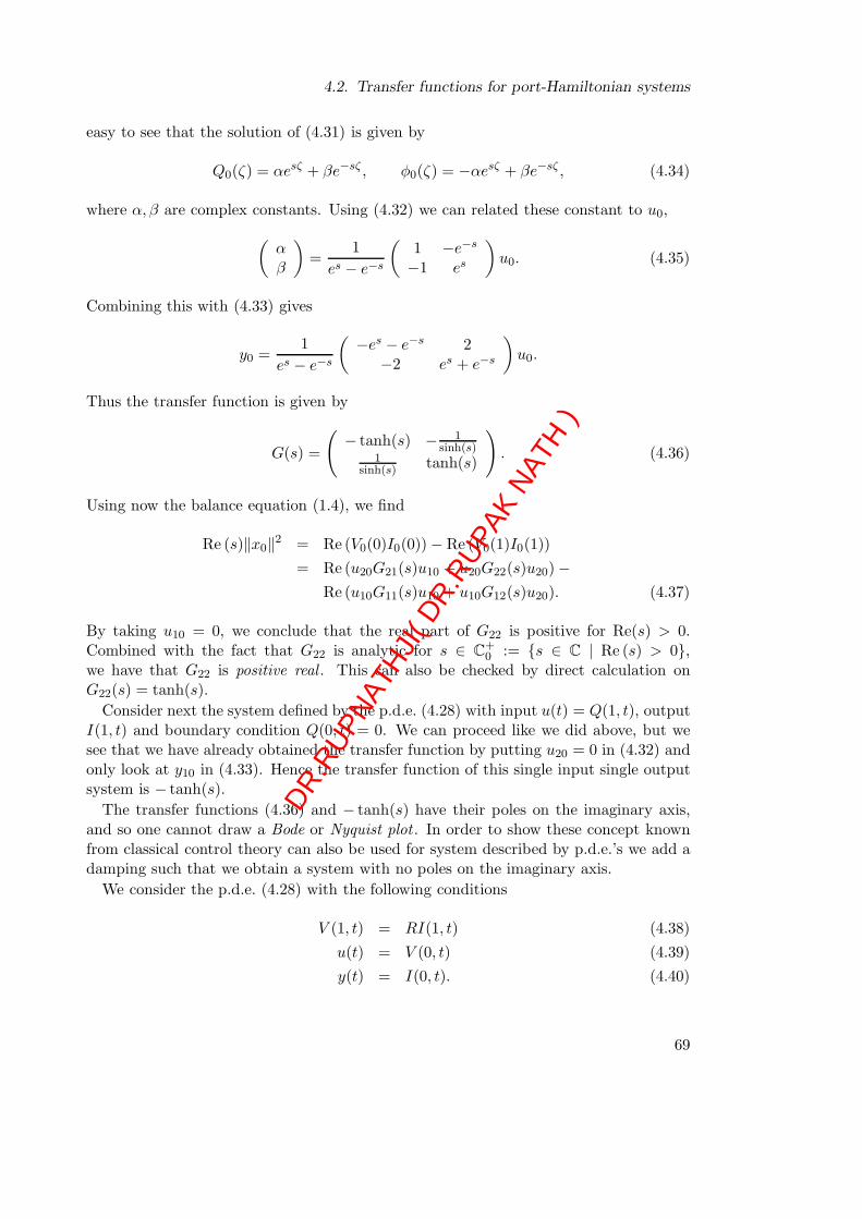
4.2. Transfer functions for port-Hamiltonian systems

easy to see that the solution of (4.31) is given by

Q0(ζ) = αesζ + βe−sζ , φ0(ζ) = −αesζ + βe−sζ , (4.34)

where α, β are complex constants. Using (4.32) we can related these constant to u0,

(αβ

)=

1

es − e−s

(1 −e−s−1 es

)u0. (4.35)

Combining this with (4.33) gives

y0 =1

es − e−s

(−es − e−s 2

−2 es + e−s

)u0.

Thus the transfer function is given by

G(s) =

(− tanh(s) − 1

sinh(s)1

sinh(s) tanh(s)

). (4.36)

Using now the balance equation (1.4), we find

Re (s)‖x0‖2 = Re (V0(0)I0(0)) − Re (V0(1)I0(1))

= Re (u20G21(s)u10 + u20G22(s)u20) −Re (u10G11(s)u10 + u10G12(s)u20). (4.37)

By taking u10 = 0, we conclude that the real part of G22 is positive for Re(s) > 0.Combined with the fact that G22 is analytic for s ∈ C+

0 := s ∈ C | Re (s) > 0,we have that G22 is positive real . This can also be checked by direct calculation onG22(s) = tanh(s).

Consider next the system defined by the p.d.e. (4.28) with input u(t) = Q(1, t), outputI(1, t) and boundary condition Q(0, t) = 0. We can proceed like we did above, but wesee that we have already obtained the transfer function by putting u20 = 0 in (4.32) andonly look at y10 in (4.33). Hence the transfer function of this single input single outputsystem is − tanh(s).

The transfer functions (4.36) and − tanh(s) have their poles on the imaginary axis,and so one cannot draw a Bode or Nyquist plot . In order to show these concept knownfrom classical control theory can also be used for system described by p.d.e.’s we add adamping such that we obtain a system with no poles on the imaginary axis.

We consider the p.d.e. (4.28) with the following conditions

V (1, t) = RI(1, t) (4.38)

u(t) = V (0, t) (4.39)

y(t) = I(0, t). (4.40)

69

DR.RUPN

ATHJI(

DR.R

UPAK

NATH )

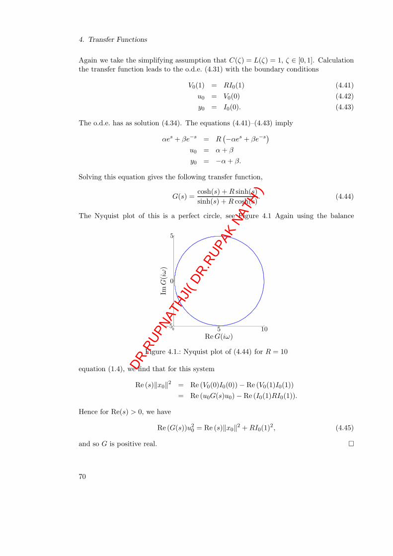
4. Transfer Functions

Again we take the simplifying assumption that C(ζ) = L(ζ) = 1, ζ ∈ [0, 1]. Calculationthe transfer function leads to the o.d.e. (4.31) with the boundary conditions

V0(1) = RI0(1) (4.41)

u0 = V0(0) (4.42)

y0 = I0(0). (4.43)

The o.d.e. has as solution (4.34). The equations (4.41)–(4.43) imply

αes + βe−s = R(−αes + βe−s

)

u0 = α+ β

y0 = −α+ β.

Solving this equation gives the following transfer function,

G(s) =cosh(s) +R sinh(s)

sinh(s) +R cosh(s). (4.44)

The Nyquist plot of this is a perfect circle, see Figure 4.1 Again using the balance

0

ReG(iω)

ImG

(iω)

0

5

5 10−5

Figure 4.1.: Nyquist plot of (4.44) for R = 10

equation (1.4), we find that for this system

Re (s)‖x0‖2 = Re (V0(0)I0(0)) − Re (V0(1)I0(1))

= Re (u0G(s)u0) − Re (I0(1)RI0(1)).

Hence for Re(s) > 0, we have

Re (G(s))u20 = Re (s)‖x0‖2 +RI0(1)

2, (4.45)

and so G is positive real.

70

DR.RUPN

ATHJI(

DR.R

UPAK

NATH )

4.3. Exercises

4.3. Exercises

4.1. Show that the assumption of Lemma 4.1.2 holds for the system (4.6)–(4.7), when-ever s ∈ ρ(A).

4.2. Show that the assumption of Lemma 4.1.2 holds for the system (4.14), whenevers ∈ ρ(A).

4.3. Determine the transfer function of the system

∂x

∂t(ζ, t) =

∂λx

∂ζ(ζ, t), ζ ∈ [a, b], t ≥ 0 (4.46)

x(ζ, 0) = x0(ζ), ζ ∈ [0, 1]

u(t) = λ(b)x(b, t), t ≥ 0.

y(t) = λ(a)x(a, t), t ≥ 0,

where λ is a (strictly) positive continuous function not depending on t.

4.4. Consider the system of the transmission line given by (4.28)–(4.30).

a) Show that even when the physical parameter C and L are spatial dependent,the equality (4.37) still holds.

b) Choose L(ζ) = eζ , and C(ζ) = 1, and determine the transfer function.

Hint: You may use a computer package like Maple or Mathematica.

4.5. Our standard port-Hamiltonian system is defined on the spatial interval [a, b].In Exercise 2.10 we have shown that it can easily be transformed to a port-Hamiltonian system on the spatial interval [0, 1]. How does the transfer functionchange?

4.6. Show that the boundary control system (4.14) defines a linear and time-invariantsystem, see below Definition 4.1.1.

4.7. Show that the Nyquist plot of transfer function (4.44) is a circle. Furthermore,show that G restricted to the imaginary axis is periodic, and determine the period.

4.8. Consider the vibrating string of Example 1.1.2. We assume that the mass densityand Young’s modulus are constant. We control this system by controlling the

velocity at ζ = b and the strain at ζ = a, i.e., u(t) =

(∂w∂t

(t,b)∂w∂ζ

(t,a)

). We observe the

same quantities, but at the opposite ends, i.e., y(t) =

(∂w∂t

(t,a)∂w∂ζ

(t,b)

).

Determine the transfer function of this system.

4.9. Since we have defined transfer functions via a different way, it may be good tocheck some well-known property of it. Let S1 and S2 be two linear and time-invariant systems, with input-output pair u1, y1 and u2, y2, respectively. Assumethat for a given s ∈ C both systems have a transfer function.

71

DR.RUPN

ATHJI(

DR.R

UPAK

NATH )

4. Transfer Functions

a) Show that the series connection, i.e., u2 = y2 has the transfer function G(s) =G2(s)G1(s).

b) Show that the parallel connection, i.e., u1 = u2 = u, and y = y1 + y2 has thetransfer function G1(s) +G2(s).

c) Show that the feedback connection, i.e., u1 = u− y2, y = y1 has the transferfunction G1(s) [I +G2(s)]

−1 provided I +G2(s) is invertible.

4.10. Consider the coupled strings of Exercise 3.8. As input we apply a force to the barin the middle, and as output we measure the velocity of this bar. Assuming thatall physical parameters are not depending on ζ, determine the transfer function.

4.4. Notes and references

The ideas for defining the transfer function in the way we did is old, but has hardlybeen investigated for distributed parameter system. [32] was the first paper where thisapproach has been used for infinite-dimensional systems. In that paper the concept wenamed transfer function was called a characteristic function.

One may find the exponential solution in Polderman and Willems [20], where allsolutions of this type are called the exponential behavior.

72

DR.RUPN

ATHJI(

DR.R

UPAK

NATH )

Chapter 5

Well-posedness

5.1. Introduction

Consider the abstract linear differential equation

x(t) = Ax(t) +Bu(t), x(0) = x0 (5.1)

y(t) = Cx(t) +Du(t). (5.2)

where x is assumed to take values in the Hilbert space X, u in the Hilbert space U , andy is the Hilbert space Y . The operator A is assumed to be the infinitesimal generatorof a C0-semigroup, and B,C, and D are bounded linear operators. Under these as-sumptions we know that the abstract differential equation (5.1)–(5.2) possesses for everyu ∈ L2((0, tf );U) a unique (mild) solution, see Theorem 3.4.1. Existence of solutionsfor an arbitrary initial condition x0 ∈ X and input u ∈ L2((0, tf );U), such that x iscontinuous and y ∈ L2((0, tf );Y ) will be called well-posedness. Hence if B,C, and Dare bounded linear operators, then the system (5.1)–(5.2) is well-posed if and only if Ais the infinitesimal generator of a C0-semigroup.

As we have seen in Chapter 3 our class of port-Hamiltonian systems cannot be writtenin the format (5.1)–(5.2) with B,C and D bounded. However, we know that for everyinitial condition and every smooth input function we have a mild solution of the statedifferential equation, see (3.14). Furthermore, for smooth initial conditions and smoothinputs, the output equation is well-defined, see Theorem 3.4.2. Note that this was onlyobtained under the condition WBΣW T

B ≥ 0. This inequality is equivalent to the factthat we have a contraction semigroup, see Theorem 2.3.2. That a larger class of inputsmight be possible, can be seen in the following example.

Consider the controlled transport equation on the interval [0, 1] with scalar controland observation on the boundary

∂x

∂t(ζ, t) =

∂x

∂ζ(ζ, t), x(ζ, 0) = x0(ζ), ζ ∈ [0, 1] (5.3)

u(t) = x(1, t), (5.4)

y(t) = x(0, t). (5.5)

73

DR.RUPN

ATHJI(

DR.R

UPAK

NATH )

5. Well-posedness

From Example 3.2.3 we know that the mild solution of (5.3)–(5.4) is given by

x(ζ, t) =

x0(ζ + t) ζ + t ≤ 1

u(ζ + t− 1) ζ + t > 1.(5.6)

We see that for every t ≥ 0 the function x(·, t) ∈ X = L2(0, 1), whenever u ∈ L2(0, tf ).Furthermore, x(·, t) is a continuous function in t, i.e., ‖x(·, t) − x((·, t + h) converges tozero when h converges to zero, see Exercise 5.1. Hence the mild solution (5.6) can beextended from controls in H1(0, tf ) to L2(0, tf ). If x0 and u are smooth, then we clearlysee that y(t) is well-defined for every t ≥ 0 and it is given by

y(t) =

x0(t) 0 ≤ t ≤ 1

u(t− 1) t > 1.(5.7)

However, when x0 ∈ L2(0, 1) and u ∈ L2(0, tf ), the expression (5.7) still gives that y iswell-defined as an L2-function.

Summarizing, we see that we can define a (mild) solution for (5.3)–(5.5) for all x0 ∈ Xand all u ∈ L2(0, tf ). This solution gives a state trajectory in the state space which iscontinuous, and an output trajectory which is square integrable on every compact timeinterval. Hence this system is well-posed.

Suppose next that we are applying a feedback of the form u(t) = 2y(t), this leads tothe new p.d.e.

∂x

∂t(ζ, t) =

∂x

∂ζ(ζ, t), x(ζ, 0) = x0(ζ), ζ ∈ [0, 1] (5.8)

x(1, t) = 2x(0, t). (5.9)

We would like to know whether the system has a unique (mild) solution, and so we tryto apply Theorem 2.3.2. From Example 2.3.3 we have that the boundary effort and floware given by

f∂ =1√2[x(1) + x(0)], e∂ =

1√2[x(1) − x(0)].

Hence the boundary condition (5.9) can be written as f∂ − 3e∂ = 0, i.e., WB = (1,−3).Calculation WBΣW T

B gives −6. Since this is negative, we know by Theorem 2.3.2)that the operator associated to the p.d.e. (5.8)–(5.9) does not generate a contractionsemigroup. However, it does generate a C0-semigroup. It is not hard to see that thesolution of (5.8)–(5.9) is given by

x(ζ, t) = 2n+1x0(τ), (5.10)

where ζ + t = n+ τ , τ ∈ [0, 1], n ∈ N, see Exercise 5.2.Concluding, we see from this very simple port-Hamiltonian system that the class of

controls can be extended, and that it is possible to have a semigroup, even when thecondition WBΣW T

B ≥ 0 is not satisfied. The aim of this chapter is to show that theseresults hold for any port-Hamiltonian system in our class.

74

DR.RUPN

ATHJI(

DR.R

UPAK

NATH )

5.2. Well-posedness for port-Hamiltonian systems

5.2. Well-posedness for port-Hamiltonian systems

In this section we define formally what we mean by well-posedness. Although well-posedness can be defined very generally, see the Notes and reference section, we do itfor our class of systems introduced in Sections 3.3 and 3.4.

∂x

∂t(ζ, t) = P1

∂

∂ζ[Hx(t)] + P0[Hx(t)] (5.11)

u(t) = WB,1

(f∂(t)e∂(t)

)(5.12)

0 = WB,2

(f∂(t)e∂(t)

)(5.13)

y(t) = WC

(f∂(t)e∂(t)

). (5.14)

The precise assumptions on this system will be given in Theorem 5.2.6. However, asbefore, we assume that H is a symmetric n×n matrix satisfying 0 < mI ≤ H(ζ) ≤MI.

Furthermore, WB :=(WB,1

WB,2

)is a full rank matrix of size n× 2n. We assume that WB,1

is a k × 2n matrix. Our state space is the Hilbert space X = L2((a, b); Rn) with theinner product

〈f, g〉X =1

2

∫ b

af(ζ)TH(ζ)g(ζ)d ζ. (5.15)

The following lemma follows easily from Theorems 3.3.1 and 3.4.2. The proof is leftas an exercise, see Exercise 5.3.

Lemma 5.2.1. Let tf be a positive real number. Assume that the operator A definedas P1

∂∂ζH + P0H with domain,

D(A) = x0 ∈ X | Hx0 ∈ H1((a, b); Rn),WB

(f∂,0e∂,0

)= 0

is the infinitesimal generator of a C0-semigroup on X. Then the system (5.11)–(5.13) isa boundary control system.

In particular, for every Hx0 ∈ H1((a, b); Rn) and every u(·) ∈ C2([0, tf ); Rk) with

u(0) = WB,1

(f∂,0e∂,0

), and 0 = WB,2

(f∂,0e∂,0

), there exists a unique classical solution of

(5.11)–(5.13) on [0, tf ]. Furthermore, the output (5.14) is well-defined and y(·) is con-tinuous on [0, tf ].

This lemma tells us that under the existence assumption of a semigroup, we have asolution for smooth inputs and initial conditions. The concept of well-posedness impliesthat we have solutions for every initial condition and every square integrable input.

Definition 5.2.2. Consider the system (5.11)–(5.14) and let k be the dimension of u.This system is well-posed if there exists a tf > 0 and mf ≥ 0 such that the followingholds:

75

DR.RUPN

ATHJI(

DR.R

UPAK

NATH )

5. Well-posedness

1. The operator A defined as P1∂∂ζH + P0H with domain,

D(A) = x0 ∈ X | Hx0 ∈ H1((a, b); Rn),WB

(f∂,0e∂,0

)= 0 (5.16)

is the infinitesimal generator of a C0-semigroup on X.

2. The following inequality holds for all Hx0 ∈ H1((a, b); Rn) and u ∈ C2([0, tf ); Rk)

with u(0) = WB,1

(f∂,0e∂,0

), and 0 = WB,2

(f∂,0e∂,0

)

‖x(tf )‖2X +

∫ tf

0‖y(t)‖2dt ≤ mf

[‖x0‖2

X +

∫ tf

0‖u(t)‖2dt

]. (5.17)

♣If the system is well-posed, then we can define a (mild) solution of (5.11)–(5.14) for

all x0 ∈ X and u ∈ L2((0, tf ),Rk) such that x(t) is a continuous function in X and y is

square integrable.

Theorem 5.2.3. If the system (5.11)–(5.14) is well-posed, then the mild solution (3.14)can be extended to hold for all u ∈ L2((0, tf ); R

k). Furthermore, the state trajectoryremains continuous, and the output is square integrable.

For the (extended) solution, the inequality (5.17) holds.Furthermore, if the system is well-posed for some tf > 0, then it is well-posed for all

tf > 0.

Proof: See Section 5.6.

As we have seen in Chapter 4, the system (5.11)–(5.14) has a transfer function. FromTheorem 4.1.4 we conclude that this function exists in the resolvent set of A. Since Agenerates a C0-semigroup, this resolvent set contains a right half-plane. So the transferfunction exists on some right-half plane. Furthermore, the transfer function is boundedfor Re(s) → ∞.

Lemma 5.2.4. Let G be the transfer function of a well-posed system, then

lim supRe(s)→∞

‖G(s)‖ ≤ √mf , (5.18)

where mf is the constant from equation (5.17).

Proof: If (5.18) does not hold, then we can find an s such that |e2stf | > mf and‖G(s)‖ > √

mf . Next choose u0 ∈ U such that ‖u0‖ = 1 and ‖G(s)u0‖ = ‖G(s)‖. Theexponential solution (u0e

st, x0est, G(s)u0e

st) satisfies

‖x(tf )‖2X +

∫ tf

0‖y(t)‖2dt = ‖x(tf )‖2

X +

∫ tf

0‖G(s)u0e

st‖2dt

= |e2stf |‖x0‖2X + ‖G(s)‖2

∫ tf

0‖estu0‖2dt

> mf

[‖x0‖2

X +

∫ tf

0‖u(t)‖2dt

].

This contradicts (5.17), and so (5.18) must hold.

76

DR.RUPN

ATHJI(

DR.R

UPAK

NATH )

5.2. Well-posedness for port-Hamiltonian systems

Although the transfer function is bounded on some right half-plane, this does notimply that it will converge along the real axis. If this happens, we call the transferfunction regular.

Definition 5.2.5. Let G(s) be the transfer function of (5.11)–(5.14). The system(5.11)–(5.14) is regular when lims∈R,s→∞G(s) exists. If the system (5.11)–(5.14) isregular, then the feed-through term D is defined as D = lims∈R,s→∞G(s). ♣

Now we have all the ingredients to formulate the main result of this chapter.

Theorem 5.2.6. Consider the partial differential equation (5.11)–(5.14) on the spatialinterval [a, b], with x(ζ, t) taking values in Rn. Let X be the Hilbert space L2((a, b); Rn)with inner product (5.15). Furthermore, assume that

• P1 is real-valued, invertible, and symmetric, i.e., P T1 = P1,

• H(ζ) is a (real) symmetric matrix satisfying 0 < mI ≤ H(ζ) ≤MI, ζ ∈ [a, b].

• The multiplication operator P1H can be written as

P1H(ζ) = S−1(ζ)∆(ζ)S(ζ), (5.19)

with ∆(·) a diagonal multiplication operator, and both ∆(·) and S(·) are continu-ously differentiable,

• WB :=(WB,1

WB,2

)is a n× 2n matrix with rank n,

• rank

(WB,1

WB,2

WC

)= n+ rank (WC).

If the homogeneous p.d.e., i.e., u ≡ 0, generates a C0-semigroup on X, then the sys-tem (5.11)–(5.14) is well-posed, and the corresponding transfer function G is regular.Furthermore, we have that limRe(s)→∞G(s) = lims→∞,s∈RG(s).

This theorem tells us that if A defined in Lemma 5.2.1 generates a C0-semigroup, thenthe system is well-posed. In particular, we have a mild solution for all square integrableinputs. From Chapter 2 we know that if WBΣW T

B ≥ 0, then A generates a (contraction)semigroup, and so in this situation the system is well-posed.

In the coming sections we prove this result. Here we comment on the conditions.

• The first two conditions are very standard, and are assumed to be satisfied for allour port-Hamiltonian systems until now.

• Note that we do not have a condition on P0. In fact the term P0H may be replacedby any bounded operator on X, see Lemma 5.4.1.

• The third condition is not very strong, and will almost always be satisfied if H(·) iscontinuously differentiable. Note that ∆ contains the eigenvalues of P1H, whereasS−1 contains the eigenvectors.

77

DR.RUPN

ATHJI(

DR.R

UPAK

NATH )

5. Well-posedness

• The fourth condition tells us that we have n boundary conditions, when we putthe input to zero. This very logical, since we have an n’th order p.d.e.

• The last condition tells that we are not measuring quantities that are set to zero,or set to be an input. This condition is not important for the proof, and willnormally follow from correct modeling.

As mentioned, the third condition is not very strong. We prove some properties of ∆next.

Lemma 5.2.7. Let P1 and H satisfy the conditions of Theorem 5.2.6. Then ∆ can bewritten as

∆(ζ) =

(Λ(ζ) 0

0 Θ(ζ)

), (5.20)

where Λ(·) is a diagonal (real) matrix, with (strictly) positive functions on the diagonal,and Θ(·) is a diagonal (real) matrix, with (strictly) negative functions on the diagonal.

Proof: Let ζ ∈ [a, b] be fixed. Since H(ζ) > mI, we can take the square root of it. By

the law of inertia, we know that the inertia of H(ζ)12P1H(ζ)

12 equals the inertia of P1.

This implies that the inertia of H(z)12P1H(ζ)

12 is independent of ζ. Furthermore, since

P1 is invertible, we conclude that the number of negative eigenvalues of H(z)12P1H(ζ)

12

equals the number of negative eigenvalues of P1. A similar statement holds for thepositive eigenvalues.

A simple calculation gives that the eigenvalues of H(ζ)12P1H(ζ)

12 are equal to the

eigenvalues of P1H(ζ). Concluding, we see that for all ζ ∈ [a, b] zero is not an eigenvalueof P1H(ζ), and that the number of negative and positive eigenvalues of P1H(ζ) is inde-pendent of ζ. We can regroup the eigenvalues such that first are positive. By doing so,we obtain (5.20).

We illustrate the conditions in the theorem by proving that they are easily satisfiedfor the example of the wave equation. From Example 1.1.2 together with (1.20) we knowthat the model of the wave equation written in the port-Hamiltonian form is given by

∂

∂t

(x1(ζ, t)x2(ζ, t)

)=

(0 11 0

)∂

∂ζ

[( 1ρ(ζ) 0

0 T (ζ)

)(x1(ζ, t)x2(ζ, t)

)], (5.21)

where x1 = ρ∂w∂t is the momentum and x2 = ∂w∂ζ is the strain.

Hence we have that

P1 =

(0 11 0

), H(ζ) =

( 1ρ(ζ) 0

0 T (ζ)

).

Being physical constants, the Young’s modulus T and the mass density ρ are positive.Hence it is clear that P1 and H satisfy the first two conditions of Theorem 5.2.6. Weshall show that (5.19) holds.

P1H(ζ) =

(0 T (ζ)1ρ(ζ) 0

). (5.22)

78

DR.RUPN

ATHJI(

DR.R

UPAK

NATH )

5.3. The operator P1H is diagonal.

satisfies the third condition, i.e., relation (5.19). The eigenvalues of this matrix are ±γwith γ(ζ) = T (ζ)

ρ(ζ) . The corresponding eigenvectors are

(γ(ζ)

1ρ(ζ)

)and

( −γ(ζ)1ρ(ζ)

). (5.23)

Hence

P1H = S−1∆S =

(γ −γ1ρ

1ρ

)(γ 00 −γ

)( 12γ

ρ2

−12γ

ρ2

), (5.24)

where we have omitted the dependence on ζ. The idea of the proof is the following.Since S is invertible, well-posedness will not change if we perform a basis transformation,x = Sx. After this basis transformation, the p.d.e. becomes

∂x

∂t(ζ, t) =

∂

∂ζ(∆x) (ζ, t) + S(ζ)

dS−1(ζ)

dζ∆(ζ)x(ζ, t)

=∂

∂ζ

(γ(ζ)x1(ζ, t)−γ(ζ)x2(ζ, t)

)+ S(ζ)

dS−1(ζ)

dζ∆(ζ)x(ζ, t). (5.25)

We see that we have a very nice set of simple p.d.e.’s, just two simple delay line, but

they are corrupted by the term S(ζ)dS−1(ζ)dζ ∆(ζ)x(ζ, t). We first assume that this term

is not present, and so we study the well-posedness of the collection of delay lines

∂

∂t

(x1(ζ, t)x2(ζ, t)

)=

∂

∂ζ

(γ(ζ)x1(ζ, t)−γ(ζ)x2(ζ, t)

)(5.26)

Although it seems that these p.d.e.’s are uncoupled, they are coupled via the boundaryconditions. In Section 5.3 we investigate when a p.d.e. like the one given in (5.26) withcontrol and observation at the boundary is well-posed. In Section 5.4 we return to theoriginal p.d.e., and show that ignoring bonded terms, like we did in (5.25) and (5.26)does not influence the well-posedness of the system. Since a basis transformation doesnot effect it either, we have proved Theorem 5.2.6.

5.3. The operator P1H is diagonal.

In this section, we prove Theorem 5.2.6 if P1H is diagonal, i.e., when S = I. For thiswe need the following two lemma’s.

Lemma 5.3.1. Let λ(ζ) be a positive continuous differentiable function on the interval[a, b]. With this function we define the scalar system

∂w

∂t(ζ, t) =

∂

∂ζ(λ(ζ)w(ζ, t)) , w(ζ, 0) = w0(ζ) ζ ∈ [a, b] (5.27)

The value at b we choose as input

u(t) = λ(b)w(b, t) (5.28)

79

DR.RUPN

ATHJI(

DR.R

UPAK

NATH )

5. Well-posedness

and as output we choose the value on the other end

y(t) = λ(a)w(a, t). (5.29)

The system (5.27)–(5.29) is a well-posed system on the state space L2(a, b). Its transferfunction is given by

G(s) = e−p(b)s, (5.30)

where p is defined as

p(ζ) =

∫ ζ

aλ(ζ)−1dζ ζ ∈ [a, b]. (5.31)

This transfer function satisfies

limRe(s)→∞

G(s) = 0. (5.32)

Proof: It is easy to see that the system (5.27)–(5.29) is a very simple version of the

general Port-Hamiltonian system (3.32)–(3.34) with P1 = 1, H = λ, WB = (√

22 ,

√2

2 ) and

WC = (√

22 ,−

√2

2 ), see Exercise 5.4. Since WBΣW TB = 1 > 0, we conclude by Theorem

3.4.2 that (5.27)–(5.29) has a well-defined solution provided the initial condition and theinput are smooth. For this class, the balance equation (3.36) holds. However, this is thesame as (1.27). Using that form of the power balance, we obtain

d

dt

∫ b

aw(ζ, t)λ(ζ)w(ζ, t)dζ = [[λ(ζ)w(ζ, t)] λ(ζ)w(ζ, t)]ba

= |u(t)|2 − |y(t)|2,

where we used (5.28) and (5.29). Thus for all tf > 0 we have that

∫ b

aw(ζ, tf )λ(ζ)w(ζ, tf )dζ−

∫ b

aw(ζ, 0)λ(ζ)w(ζ, 0)dζ

=

∫ tf

0|u(τ)|2dτ −

∫ tf

0|y(τ)|2dτ. (5.33)

Since λ is strictly positive, we have that the energy norm∫ ba w(ζ, t)λ(ζ)w(ζ, t)dζ is

equivalent to the L2(a, b)-norm, and so on a dense set an inequality like (5.17) is satisfied.Thus the system is well-posed.

As we have seen in Chapter 4, the transfer function G(s) is constructed by findingfor s ∈ C and for all u0 a triple (us(t), ws(ζ, t), y(t)) = (u0e

st, w0(ζ)est, y0e

st) satisfying(5.27)–(5.29). Substituting a triple of this form in the p.d.e., gives

sw0(ζ) =∂

∂ζ(λ(ζ)w0(ζ)) , u0 = λ(b)w0(b), y0 = λ(a)w0(a).

Thus w0(ζ) = u0λ(ζ)−1 exp(s(p(ζ)−p(b))), and y0 = u0 exp(−sp(b)). This proves (5.30).The property (5.32) follows directly from (5.30) and the fact that p(b) > 0.

80

DR.RUPN

ATHJI(

DR.R

UPAK

NATH )

5.3. The operator P1H is diagonal.

For a p.d.e. with negative coefficient, we obtain a similar result.

Lemma 5.3.2. Let θ(ζ) be a negative continuous function on the interval [a, b]. Withthis function we define the scalar system

∂w

∂t(ζ, t) =

∂

∂z(θ(ζ)w(ζ, t)) , w(ζ, 0) = w0(ζ) ζ ∈ [a, b] (5.34)

The value at a we choose as input

u(t) = θ(a)w(a, t) (5.35)

and as output we choose the value on the other end

y(t) = θ(b)w(b, t). (5.36)

The system (5.34)–(5.36) is a well-posed system on the state space L2(a, b). Its transferfunction is given by

G(s) = en(b)s, (5.37)

where

n(ζ) =

∫ ζ

aθ(ζ)−1dζ, ζ ∈ [a, b]. (5.38)

This transfer function satisfies

limRe(s)→∞

G(s) = 0. (5.39)

We use these two lemmas to prove Theorem 5.2.6 when P1H is diagonal and the inputspace has dimension n.

Consider the following diagonal hyperbolic system on the spatial interval ζ ∈ [a, b]

∂

∂t

(x+(ζ, t)x−(ζ, t)

)=

∂

∂ζ

[(Λ(ζ) 0

0 Θ(ζ)

)(x+(ζ, t)x−(ζ, t)

)](5.40)

where Λ(ζ) is a diagonal (real) matrix, with positive functions on the diagonal, and Θ(ζ)is a diagonal (real) matrix, with negative functions on the diagonal. Furthermore, weassume that Λ and Θ are continuously differentiable.

With this p.d.e. we associate the following boundary control and observation

us(t) :=

(Λ(b)x+(b, t)Θ(a)x−(a, t)

), (5.41)

ys(t) :=

(Λ(a)x+(a, t)Θ(b)x−(b, t)

). (5.42)

Theorem 5.3.3. Consider the p.d.e. (5.40) with us and ys as defined in (5.41) and(5.42), respectively.

81

DR.RUPN

ATHJI(

DR.R

UPAK

NATH )

5. Well-posedness

• The system defined by (5.40)–(5.42) is well-posed and regular. Furthermore, itstransfer function converges to zero for Re(s) → ∞.

• To the p.d.e. (5.40) we define a new set of inputs and outputs. The new input u(t)is written as

u(t) = Kus(t) +Qys(t), (5.43)

where K and Q are two square matrices, with [K,Q] of rank n. The new outputis written as

y(t) = O1us(t) +O2ys(t). (5.44)

where O1 and O2 are some matrices. For the system (5.40) with input u(t) andoutput y(t), we have the following possibilities:

1. If K is invertible, then the system (5.40), (5.43), and (5.44) is well-posed andregular. Furthermore, its transfer function converges to O1K

−1 for Re(s) →∞

2. If K is not invertible, then the operator AK defined as

AK

(g+(ζ)g−(ζ)

)=

∂

∂ζ

[(Λ(ζ) 0

0 Θ(ζ)

)(g+(ζ)g−(ζ)

)](5.45)

with domain

D(AK) =

(g+(ζ)g−(ζ)

)∈ H1((a, b),Rn) |

K

(Λ(b)g+(b)Θ(a)g−(a)

)+ Q

(Λ(a)g+(a)Θ(b)g−(b)

)= 0

(5.46)

does not generate a C0-semigroup on L2((a, b); Rn).

Note that the last item implies that the homogeneous p.d.e. does not have a well-definedsolution, when K is not invertible.

Proof: The first item is a direct consequence of Lemma 5.3.1 and 5.3.2 by noticingthat the system (5.40)–(5.42) is built out of copies of the system (5.27)–(5.29) and thesystem (5.34)–(5.36). Furthermore, these sub-systems do not interact with each other.

For the proof of the first part of the second assertion, with K invertible, we rewritethe new input, as us(t) = K−1u(t) − K−1Qys(t). This can be seen as a feedbackinterconnection on the system (5.40)–(5.42), as is depicted in Figure 5.1. The systemcontains one feedback loop with gain matrix K−1Q. By Theorem 5.6.1, we have that ifI +Gs(s)K

−1Q is invertible on some right half-plane and if this inverse is bounded on aright-half plane, then the closed loop system is well-posed. Since limRe(s)→∞Gs(s) = 0,we see that this holds for everyK−1 andQ. So under the assumption thatK is invertible,we find that (5.40) with input and output given by (5.43) and (5.44) is well-posed. Theregularity follows easily. By regarding the loops in Figure 5.1, we see that the feed-thoughterm is O1K

−1.

82

DR.RUPN

ATHJI(

DR.R

UPAK

NATH )

5.3. The operator P1H is diagonal.

−u(t)

us(t)

y(t)

ys(t)Gs(s)

Q

K−1 O2

O1

Figure 5.1.: The system (5.40) with input (5.43) and output (5.44)

So it remains to show that there is no C0-semigroup when K is non-invertible. SinceK is singular, there exists a non-zero v ∈ Rn such that vTK = 0. Since [K,Q] has fullrank, we know that qT := vTQ 6= 0. So at least one of the components of q is unequalto zero. For the sake of the argument, we assume that this holds for the first one.

If AK would be the infinitesimal generator of a C0-semigroup, then for all x0 ∈ D(AK)the abstract differential equation

x(t) = AKx(t), x(0) = x0 (5.47)

would have classical solution, i.e., for all t > 0, x(t) is differentiable, it is an element ofD(AK), and it satisfies (5.47). Hence by (5.46), we have that x(t) is an element of H1.Since we are working in a one dimensional spatial domain, we have that functions in H1

are continuous. So we have that for every t, x(t) is a continuous function of ζ satisfyingthe boundary conditions in (5.46).

So if AK would generate a C0-semigroup, then for every x0 ∈ D(AK) there would be a

function x(ζ, t) :=(x+(ζ,t)x−(ζ,t)

)which is a (mild) solution to the p.d.e. (5.40), and satisfies

for all t > 0 the boundary condition

K

(Λ(b)x+(b, t)Θ(a)x−(a, t)

)+Q

(Λ(a)x+(a, t)Θ(b)x−(b, t)

)= 0.

Using the vectors v and q, we see that this x(ζ, t) must satisfy

0 = qT(

Λ(a)x+(a, t)Θ(b)x−(b, t)

), t > 0. (5.48)

Now we construct an initial condition in D(AK), for which this equality does not hold.Note that we have chosen the first component of q unequal to zero.

The initial condition x0 is chosen to have all components zero except for the first one.For this first component we choose an arbitrary function in H1(a, b) which is zero at aand b, but nonzero everywhere else on the open set (a, b). It is clear that this initialcondition is in the domain of AK . Now we solve (5.40).

Standard p.d.e. theory gives that the solution of (5.40) can be written as

x+,m(ζ, t) = f+,m(pm(ζ) + t)λm(ζ)−1, (5.49)

x−,ℓ(ζ, t) = f−,ℓ(nℓ(ζ) + t)θℓ(ζ)−1, (5.50)

83

DR.RUPN

ATHJI(

DR.R

UPAK

NATH )

5. Well-posedness

where λm and θℓ are the m-th and the ℓ-th diagonal element of Λ and Θ, respectively.Furthermore, pm(ζ) =

∫ ζa λm(ζ)−1dζ, nl(ζ) =

∫ ζa θl(ζ)

−1dζ, see also Exercises 5.4 and5.5. The functions f+, f− need to be determined from the boundary and initial condi-tions.

Using the initial condition we have that f+,m(pm(ζ)) = λm(ζ)x0,+,m(ζ) and f−,ℓ(nℓ(ζ)) =θℓ(ζ)x0,−,ℓ(ζ). Since pm > 0, and nℓ < 0, we see that the initial condition determines f+

on a (small) positive interval, and f− on a small negative interval. By our choice of theinitial condition, we find that

f+,1(ξ) = λ1(ξ)x0,+,1(ξ) ξ ∈ [0, p1(b)),

f+,m(ξ) = 0 ξ ∈ [0, pm(b)), m ≥ 2, (5.51)

f−,ℓ(ξ) = 0 ξ ∈ [nℓ(b), 0), ℓ ≥ 1.

The solution x(ζ, t) must also satisfy (5.48), thus for all t > 0 we have that

0 = qT(

f+(t)f−(n(b) + t)

)(5.52)

Combining this with (5.51), we find

0 = q1f+,1(p1(ζ)) = q1x0,+,1(ζ)λ−11 (ζ)

on some interval [a, β]. Since q1 and λ1 are unequal to zero, we find that x0 must bezero on some interval. This is in contradiction with our choice of the initial condition.Thus AK cannot be the infinitesimal generator of a C0-semigroup.

5.4. Proof of Theorem 5.2.6.

In this section we use the results of the previous section to prove Theorem 5.2.6. Webegin with a useful lemma, which proof can be found in Section 5.6.

Lemma 5.4.1. The system (5.11)–(5.14) is well-posed if and only if the system

∂x

∂t(ζ, t) = P1

∂

∂ζ(Hx) (ζ, t), (5.53)

with inputs, outputs given by (5.12)–(5.14) is well-posed.

Let G(s) denote the transfer function of (5.11)–(5.14) and G0(s) the transfer functionof (5.53) with (5.12)–(5.14). Then

lims→∞

G(s) = lims→∞

G0(s), (5.54)

and

limRe(s)→∞

G(s) = limRe(s)→∞

G0(s), (5.55)

84

DR.RUPN

ATHJI(

DR.R

UPAK

NATH )

5.4. Proof of Theorem 5.2.6.

This lemma tells us that we may ignore any bounded linear term involving x.Now we have all the results needed to prove Theorem 5.2.6.By the third assumption of Theorem 5.2.6, the matrices P1 and H satisfy the equation

(5.19):P1H(ζ) = S−1(ζ)∆(ζ)S(ζ).

With this we introduce the new state vector

x(ζ, t) = S(ζ)x(ζ, t), ζ ∈ [a, b] (5.56)

Under this basis transformation, the p.d.e. (5.11) becomes

∂x

∂t(ζ, t) =

∂

∂ζ(∆x) (ζ, t) + S(ζ)

dS−1(ζ)

dζ∆(ζ)x(ζ, t)+

S(ζ)P0(ζ)S(ζ)−1x(ζ, t), x(ζ, 0) = S(ζ)x0(ζ) = x0(ζ). (5.57)

The relations (5.12)–(5.14) become

0 =M11P−11 S−1(b)∆(b)x(b, t) +M12P

−11 S−1(a)∆(a)x(a, t)

=M11∆(b)x(b, t) + M12∆(a)x(a, t) (5.58)

u(t) =M21P−11 S−1(b)∆(b)x(b, t) +M22P

−11 S−1(a)∆(a)x(a, t)

=M21∆(b)x(b, t) + M22∆(a)x(a, t) (5.59)

y(t) =C1P−11 S−1(b)∆(b)x(b, t) + C2P

−11 S−1(a)∆(a)x(a, t)

=C1∆(b)x(b, t) + C2∆(a)x(a, t). (5.60)

We introduce M =(M11 M12

M21 M22

)with

(Mj1 Mj2

)=(Mj1 Mj2

)( P−11 S(b)−1 0

0 P−11 S(a)−1

), j = 1, 2.

and

C =(C1 C2

)=(C1 C2

)( P−11 S(b)−1 0

0 P−11 S(a)−1

).

Since the matrix(P−1

1 S(b)−1 0

0 P−11 S(a)−1

)has full rank, we see that the rank conditions in

Theorem 5.2.6 imply similar rank conditions for M and C.Using Lemma 5.4.1 we see that we only have to prove the result for the p.d.e.

∂x

∂t(ζ, t) =

∂

∂ζ(∆x) (ζ, t). (5.61)

with boundary conditions, inputs, and outputs as described in (5.58)–(5.60).It is clear that if condition (5.58) is not present, then Theorem 5.3.3 gives that the

above system is well-posed and regular if and only if the homogeneous p.d.e. generates aC0-semigroup on L2((a, b); Rn). Since the state transformation (5.56) defines a bounded

85

DR.RUPN

ATHJI(

DR.R

UPAK

NATH )

5. Well-posedness

mapping on L2((a, b); Rn), we have proved Theorem 5.2.6 provided there is no condition(5.12).

Thus it remains to prove Theorem 5.2.6 if we have put part of the boundary conditionsto zero. Or equivalently, to prove that the system (5.58)–(5.61) is well-posed and regularif and only if the homogeneous p.d.e. generates a C0-semigroup.

We replace (5.58) by

v(t) = M11∆(b)x(b, t) + M12∆(a)x(a, t), (5.62)

where we regard v as a new input. Hence we have the system (5.61) with the newextended input

(v(t)u(t)

)=

(M11

M21

)∆(b)x(t, b) +

(M12

M22

)∆(a)x(t, a). (5.63)

and the output (5.60). By doing so, we have obtained a system without a condition(5.58). For this system we know that it is well-posed and regular if and only if thehomogeneous equation generates a C0-semigroup.

Assume that the system (5.61), (5.63) and (5.60) is well-posed, then we may chooseany (locally) square input. In particular, we may choose v ≡ 0. Thus the system(5.57)–(5.61) is well-posed and regular as well.

Assume next that the p.d.e. with the extended input in (5.63) set to zero, does notgenerate a C0-semigroup. Since this gives the same homogeneous p.d.e. as (5.61) with(5.58) and u in (5.59) set to zero, we know that this p.d.e. does not generate a C0-semigroup. This finally proves Theorem 5.2.6.

5.5. Well-posedness of the vibrating string.

In this section we illustrate the usefulness of Theorem 5.2.6 by applying it to the vibratingstring of Example 1.1.2.

By equation (1.20) we know that for the vibrating string there holds

P1 =

(0 11 0

), H(ζ) =

( 1ρ(ζ) 0

0 T (ζ)

).

Since we want to illustrate the theory and proofs derived in the previous sections, wedo not directly check if for a (to-be-given) set of boundary conditions the semigroupcondition is satisfied. Instead of that, we rewrite the system in its diagonal form, andcheck the conditions using Theorem 5.3.3. As we have seen in Section 5.4, the proof ofTheorem 5.2.6 follows after a basis transformation directly from Theorem 5.3.3. Hencewe start by diagonalizing P1H. Although all the results hardly change, we assume forsimplicity of notation that Young’s modulus T and the mass density ρ are constant.Being physical constants, they are naturally positive.

From equation (5.24 we know that the operator P1H is diagonalizable:

P1H = S−1∆S =

(γ −γ1ρ

1ρ

)(γ 00 −γ

)( 12γ

ρ2

−12γ

ρ2

), (5.64)

86

DR.RUPN

ATHJI(

DR.R

UPAK

NATH )

5.5. Well-posedness of the vibrating string.

where γ is positive and satisfies γ2 = c = Tρ .

Hence the state transformation under which the p.d.e. becomes diagonal is

x =1

2

(1γ ρ−1γ ρ

)x.

Since we assumed that γ > 0, we see that x1, x2 correspond to x+, and x− in equation(5.40), respectively and Λ,Θ to γ and −γ, respectively. Hence we have that the input andoutput us and ys defined for the diagonal system (5.40) by the equations (5.41)–(5.42)are expressed in the original coordinates by

us(t) =1

2

(x1(b, t) + γρx2(b, t)x1(a, t) − γρx2(a, t)

), (5.65)

ys(t) =1

2

(x1(a, t) + γρx2(a, t)x1(b, t) − γρx2(b, t)

). (5.66)

This pair of boundary input and output variables consists in complementary linear com-binations of the momentum x1 and the strain x2 at the boundaries: however they lackan obvious physical interpretation. One could consider another choice of boundary inputand outputs, for instance the velocity and the strain at the boundary points and chooseas input

u1(t) =

( x1ρ (b, t)

x2(a, t)

)(5.67)

and as output

y1(t) =

( x1ρ (a, t)

x2(b, t)

). (5.68)

We may apply Theorem 5.3.3 to check whether this system is well-posed, and to findthe feed-through. Expressing the input-output pair (u1, y1) in (us, ys) gives

u1(t) =

(1ρ 0

0 −1√Tρ

)us(t) +

(0 1

ρ1√Tρ

0

)ys(t), (5.69)

y1(t) =

(0 1

ρ1√Tρ

0

)us(t) +

(1ρ 0

0 −1√Tρ

)ys(t). (5.70)

Hence

K =

(1ρ 0

0 −1√Tρ

)Q =

(0 1

ρ1√Tρ

0

), (5.71)

O1 =

(0 1

ρ1√Tρ

0

), O2 =

(1ρ 0

0 −1√Tρ

). (5.72)

Since K is invertible, the system with the input-output pair (u1, y1) is well-posed and

regular, and the feed-through term is given by O1K−1 =

(0 −γ1γ

0

).

87

DR.RUPN

ATHJI(

DR.R

UPAK

NATH )

5. Well-posedness

Since the states are defined as x1 = ρ∂w∂t and x2 = ∂w∂ζ , the control and observation

are easily formulated using w. Namely, u1(t) =

(∂w∂t

(t,b)∂w∂ζ

(t,a)

)and y1(t) =

(∂w∂t

(t,a)∂w∂z

(t,b)

),

respectively. Hence we observe the velocity and strain at opposite ends.

Next we show that if we would control the velocity and strain at the same end, thisdoes not give a well-posed system. The control and observation are given by

u2(t) =

( ∂w∂t (b, t)∂w∂ζ (b, t)

)=

( x1ρ (b, t)

x2(b, t)

)(5.73)

and as output

y2(t) =

( ∂w∂t (a, t)∂w∂ζ (a, t)

)=

( x1ρ (a, t)

x2(a, t)

). (5.74)

It is easy to see that

u2(t) =

(1ρ 01γρ 0

)us(t) +

(0 1

ρ

0 − 1γρ

)ys(t). (5.75)

Clearly the matrix in front of us is not invertible, and hence we conclude by Theorem5.3.3 that the wave equation with the homogeneous boundary conditions u2 = 0 doesnot generate a C0-semigroup. Hence this system is not well-posed.

Until now we have been controlling velocity and strain at the end points. However,for the wave equation, it seems very naturally to control the position, i.e., w(·, t). So weconsider the wave equation (1.5) with the following control and observation.

u3(t) =

(w(b, t)∂w∂ζ (a, t)

)(5.76)

y3(t) =

(w(a, t)∂w∂z (b, t)

). (5.77)

Since the first control and first observation cannot be written as linear combination ofour boundary effort and flow, we find that this system is not of the form (5.11)–(5.14).However, we still can investigate the well-posedness of the system. For this we realizethat the first element in u3 is the time derivative of the first element of u1. So we cansee the wave equation with the input (5.76) and output (5.77) as the following seriesconnection.

u1(t)u3(t) y1(t) y3(t)G1(s)( s 0

0 1 )(s−1 00 1

)

Figure 5.2.: The wave equation with input and output (5.76) and (5.77)

88

DR.RUPN

ATHJI(

DR.R

UPAK

NATH )

5.6. Technical lemma’s

From this it is clear that the transfer function, G3(s) of the system with input u3 andoutput y3 is given by

G3(s) =

(s−1 00 1

)G1(s)

(s 00 1

).

Since for large real s the transfer function G1(s) is approximately equal to(

0 −γγ−1 0

),

we see that G3(s) grows like s for large s. By Lemma 5.2.4 we know that any well-posedsystem has a transfer function which is bounded in some right half-plane. Thus the waveequation with input (5.76) and output (5.77) is not well-posed.

The reason for the well-posedness of this system is different than for the choice u2

and y2. Since if we put u3 to zero, then this implies that u1 is zero as well, and so weknow that this homogeneous equation is well-defined and has a unique solution. So ifthe controls and/or observations are not formulated in the boundary effort and flow,then we may loose well-posedness even if there is a semigroup.

5.6. Technical lemma’s

In this section we present the proofs for the technical results which we needed. We beginby considering the boundary control system

The following result is essential in our proof, and it has been proved by G. Weiss in[30].

u(t)v(t) y(t)S

F

Figure 5.3.: The closed loop system

Theorem 5.6.1. Let S be a well-posed system with input space U and output space Y ,both being Hilbert spaces. Denote the transfer function by G(s). Let F be a boundedlinear operator from Y to U such that I −G(s)F is invertible in some right half-plane.If the inverse is bounded in a right half-plane, then the closed loop system as depictedin Figure 5.3 is again well-posed. If G is regular, then so is the closed loop transferfunction.

5.7. Exercises

5.1. Prove that the function defined by (5.6) is a continuous function in t with valuesin L2(0, 1) for any x0 ∈ L2(0, 1) and any u ∈ L2(0,∞). That is prove that

∫ 1

0|x(ζ, t) − x(ζ, t+ h)|2dζ → 0

89

DR.RUPN

ATHJI(

DR.R

UPAK

NATH )

5. Well-posedness

for h→ 0.

5.2. In this exercise we study the p.d.e. (5.8) with boundary condition (5.9).

a) Show that for an initial condition x0 which is continuously differentiable andsatisfies x0(1) = 2x0(0) the (classical) solution of (5.8)–(5.9) is given by (5.10).

b) Show that the mapping x0 7→ x(·, t) with x(ζ, t) given by (5.10) defines aC0-semigroup on L2(0, 1).

c) Conclude that (5.10) is the mild solution of (5.8)–(5.9) for any initial conditionx0 ∈ L2(0, 1).

5.3. Prove Lemma 5.2.1.

5.4. In this exercise, we show some more results for the system defined by (5.27)–(5.29).

a) Show that the system (5.27)–(5.29) is a port-Hamiltonian system of the form(3.32)–(3.34).

b) Show that the solution of (5.27)–(5.28) is given by

w(ζ, t) = f(p(ζ) + t)λ(ζ)−1, (5.78)

where

p(ζ) =

∫ ζ

aλ(ζ)−1dζ ζ ∈ [a, b] (5.79)

f(p(ζ)) = λ(ζ)w0(ζ), ζ ∈ [a, b] (5.80)

f(p(b) + t) = u(t), t > 0. (5.81)

5.5. Lemma 5.3.2: its solution is given as

w(ζ, t) = f(n(ζ) + t)θ(ζ)−1, (5.82)

where

n(ζ) =

∫ z

aθ(ζ)−1dζ (5.83)

f(n(ζ)) = θ(ζ)w0(ζ), z ∈ [a, b] (5.84)

f(t) = u(t), t > 0. (5.85)

5.6. Show that the transfer function is regular with feed-though term zero if the con-stant mf in equation (5.17) can be chosen such that mf → 0 if tf ↓ 0 for x0 = 0.

90

DR.RUPN

ATHJI(

DR.R

UPAK

NATH )

5.8. Notes and references

5.8. Notes and references

The third condition tells us that P1L is diagonalizable via a continuously differentiablebasis transformation. In Kato [14, chapter II], one can find conditions on P1L(ζ) suchthat this is possible. For simplicity, we have assumed that ∆(ζ) is continuously differ-entiable.

From the proof of Theorem 5.2.6, we see that we obtain an equivalent matrix conditionfor condition 1., i.e., item 1. of Theorem 5.2.6 holds if and only if K is invertible, seeTheorem 5.3.3. Since the matrix K is obtained after a basis transformation, and dependson the negative and positive eigenvalues of P1H, it is not easy to rewrite this conditionin a condition for Mij .

A semigroup can be extended to a group, if the homogeneous p.d.e. has for everyinitial condition a solution for negative time. Using once more the proof of Theorem5.3.3, we see that A in item 1. of Theorem 5.2.6 generates a group if and only if K andQ are invertible matrices.

That the system remains well-posed after feedback was proved by Weiss [30].This chapter is completely based on the paper by Zwart et al, [33].

91

DR.RUPN

ATHJI(

DR.R

UPAK

NATH )

5. Well-posedness

92

DR.RUPN

ATHJI(

DR.R

UPAK

NATH )

Chapter 6

Stability and Stabilizability

6.1. Introduction

In this chapter we study the stability of our systems. We study the stability of thestate, i.e., we only look at the solutions of the homogeneous differential equation. As fornon-linear systems there are two different notions of stability. Namely strong stabilityand exponential stability, which are defined next. Let A be the infinitesimal generatorof the C0-semigroup (T (t))t≥0 on the Hilbert space X. We know that x(t) := T (t)x0 isthe (unique) mild solution of the differential equation

x(t) = Ax(t), x(0) = x0. (6.1)

For the solutions we define two concepts of stability.

Definition 6.1.1. The system (6.1) is strongly stable if for every x0 ∈ X the statetrajectory x(t) converges to zero for t going to infinity. ♣

Definition 6.1.2. The system (6.1) is exponentially stable, if there exists a M > 0,ω < 0 such that

‖T (t)‖ ≤Meωt, t ≥ 0. (6.2)

♣

Since x(t) = T (t)x0, it is easy to see that exponential stability implies strong stability.The converse does not hold as is shown in the following example.

Example 6.1.3 Let X be the Hilbert space L2(0,∞) and let the C0-semigroup be givenas

(T (t)f) (ζ) = f(t+ ζ). (6.3)

As in Example 2.2.3 it is not hard to show that this is a strongly continuous semigroup.Furthermore, for all t ≥ 0 we have ‖T (t)‖ = 1, see Exercise 6.1. The later implies thatthis semigroup is not exponentially stable. It remains to show that it is strongly stable.

93

DR.RUPN

ATHJI(

DR.R

UPAK

NATH )

6. Stability and Stabilizability

Let ε > 0 and let f ∈ X = L2(0,∞). There exists a function fε such that ‖f −fε‖ ≤ εand fε(ζ) is zero for ζ sufficiently large. Let denote ζf the point from which fε(ζ) equalszero. For t > ζf , we have that T (t)fε = 0 and so

‖T (t)f‖ ≤‖T (t)f − T (t)fε‖ + ‖T (t)fε‖

=

√∫ ∞

0|f(t+ ζ) − fε(t+ ζ)|2dζ

≤√∫ ∞

0|f(z) − fε(z)|2dz ≤ ε.

Since this holds for any ε, we conclude that (T (t))t≥0 is strongly stable.

In this book we study systems in strong connection with their energy. This energyserves as our norm. In the following section we show that if the energy is decaying wehave (under mild conditions) exponential stability. We urge to say that this holds forour nice class of port-Hamiltonian system, and does not hold generally as the followingexample shows.

Example 6.1.4 In this example we construct a contraction semigroup whose norm isstrictly decreasing, but the semigroup is not strongly stable.

We take the Hilbert space L2(0,∞). However, not with its standard inner product,but we choose as inner product

〈f, g〉 =

∫ ∞

0f(ζ)g(ζ)

[e−ζ + 1

]dζ. (6.4)

As semigroup, we choose the right shift semigroup:

(T (t)f) (ζ) =

f(ζ − t) ζ > t

0 ζ ∈ [0, t)

= f(ζ − t)1[0,∞)(ζ − t).

Using the formula for the norm and the formula of the semigroup, we see that

‖T (t)f‖2 =

∫ ∞

0|f(ζ − t)1[0,∞])(ζ − t)|2

[e−ζ + 1

]dζ

=

∫ ∞

0|f(ξ)|2

[e−(ξ+t) + 1

]dξ (6.5)

≥∫ ∞

0|f(ξ)|2dξ

≥ 1

2

∫ ∞

0|f(ξ)|2

[e−ξ + 1

]dξ

=1

2‖f‖2.

94

DR.RUPN

ATHJI(

DR.R

UPAK

NATH )

6.2. Exponential stability of port-Hamiltonian systems

Hence (T (t))t≥0 cannot be strongly stable. Even more importantly, with the exceptionof f = 0, there is no initial condition for which T (t)f → 0 as t→ ∞.

Next we show that the norm of the trajectory is always decreasing. Let t2 > t1 andlet f 6= 0. From (6.5) we know that

‖T (t2)f‖2 =

∫ ∞

0|f(ξ)|2

[e−(ξ+t2) + 1

]dξ

<

∫ ∞

0|f(ξ)|2

[e−(ξ+t1) + 1

]dξ

= ‖T (t1)f‖2,

where we have used that the negative exponential is strictly decreasing. Hence the normof any trajectory is decaying, but the system is not strongly stable.

Note that the above example shows that the second method of Lyapunov1 is notdirectly applicable for p.d.e.’s2.

We end with a small technical lemma, which will be useful later on.

Lemma 6.1.5. Let (T (t))≥0 be a strongly continuous semigroup on the Hilbert spaceX. If for some t1 > 0 we have that ‖T (t1)‖ < 1, then the C0-semigroup is exponentiallystable.

Proof: If there exists a t1 > 0 such that ‖T (t1)‖ < 1, then we have that 1t1

log ‖T (t1)‖ <0. Hence ω0 = inft>0

1t log ‖T (t)‖ < 0. By Theorem 2.5.1.e, we can find a negative ω

such that ‖T (t)‖ ≤Mωeωt. Hence we have exponential stability.

In the following section we consider our class of port-Hamiltonian system, and weshow that a simple condition is guaranteeing exponential stability.

6.2. Exponential stability of port-Hamiltonian systems

We return to our homogeneous port-Hamiltonian system of Section 2.3. That is weconsider the p.d.e.

∂x

∂t(ζ, t) = P1

∂

∂ζ[H(ζ)x(ζ, t)] + P0 [H(ζ)x(ζ, t)] . (6.6)

with the boundary condition

WB

(f∂(t)e∂(t)

)= 0, (6.7)

where (f∂(t)e∂(t)

)=

1√2

(P1 −P1

I I

)((Hx) (b, t)(Hx) (a, t)

). (6.8)

As in Theorem 2.3.2 we assume that the following holds

1Given a Lyapunov function V such that V < 0, implies (asymptotic) stability2One additionally needs pre-compactness of the trajectories

95

DR.RUPN

ATHJI(

DR.R

UPAK

NATH )

6. Stability and Stabilizability

Assumption 6.2.1:

• P1 is an invertible, symmetric real n× n matrix;

• P0 is an anti-symmetric real n× n matrix;

• For all ζ ∈ [a, b] the n× n matrix H(ζ) is real, symmetric, and mI ≤ H(ζ) ≤MI,for some M,m > 0 independent of ζ;

• H is continuously differentiable on the interval [a, b];

• WB be a full rank real matrix of size n× 2n;

• WBΣW TB ≥ 0, where Σ =

(0 II 0

). ♥

The above, with the exception of the differentiability of H, have been our standardassumptions in many previous chapters. However, we would like to remark that ourmain theorem 6.2.3 also holds if P0 satisfies P0 +P T0 ≤ 0. Under the conditions as listedin Assumption 6.2.1 we know that the operator A given by

Ax := P1d

dζ[Hx] + P0 [Hx] (6.9)

with domain

D(A) = x ∈ L2((a, b); Rn) | Hx ∈ H1((a, b); Rn), WB

(f∂e∂

)= 0 (6.10)

generates a contraction semigroup on the state space

X = L2((a, b); Rn) (6.11)

with inner product

〈f, g〉X =1

2

∫ b

af(ζ)TH(ζ)g(ζ)dζ. (6.12)

In the following lemma, we show that the norm/energy of a state trajectory can bebounded by the energy at one of the boundaries. The proof is based on an idea of Coxand Zuazua in [4].

Lemma 6.2.2. Consider the generator A of the contraction semigroup (T (t))t≥0 givenby (6.9) and (6.10). Let x0 ∈ X be any initial condition, then for sufficiently large τ > 0the state trajectory x(t) := T (t)x0 satisfies

‖x(τ)‖2X ≤ c

∫ τ

0‖(Hx)(b, t)‖2 dt and (6.13)

‖x(τ)‖2X ≤ c

∫ τ

0‖(Hx)(a, t)‖2 dt, (6.14)

where c > 0 is a constant that only depends on τ and not on x0.

96

DR.RUPN

ATHJI(

DR.R

UPAK

NATH )

6.2. Exponential stability of port-Hamiltonian systems

Proof: Let x0 be an element in the domain of A and let x(t) := T (t)x0. Since x0 ∈D(A), we know that x(t) ∈ D(A) for all t. Furthermore, x(t) is the classical solution of(6.6).

For this trajectory, we define the (positive) function for ζ ∈ [a, b]

F (ζ) =

∫ τ−γ(b−ζ)

γ(b−ζ)xT (ζ, t)H(ζ)x(ζ, t) dt, (6.15)

where we assume that γ > 0 and τ > 2γ(b− a). This last condition implies that we arenot integrating over a negative time interval.

Differentiating this function with respect to ζ gives

dF

dζ(ζ) =

∫ τ−γ(b−ζ)

γ(b−ζ)xT (ζ, t)

∂

∂ζ(H(ζ)x(ζ, t)) dt+

∫ τ−γ(b−ζ)

γ(b−ζ)

(∂

∂ζx(ζ, t)

)TH(ζ)x(ζ, t) dt+

γxT (ζ, γ(b− ζ))H(ζ)x(ζ, γ(b− ζ))+

γxT (ζ, τ − γ(b− ζ))H(ζ)x(ζ, τ − γ(b− ζ)).

Since P1 is non-singular and since x satisfies (6.6), we obtain (for simplicity we omit thedependence on ζ and t)

dF

dζ(ζ) =

∫ τ−γ(b−ζ)

γ(b−ζ)xTP−1

1

(∂x

∂t− P0Hx

)dt

+ γxT (ζ, τ − γ(b− ζ))H(ζ)x(ζ, τ − γ(b− ζ))

+

∫ τ−γ(b−ζ)

γ(b−ζ)

(P−1

1

∂x

∂t− dHdζ

x− P−11 P0Hx

)Tx dt

+ γxT (ζ, γ(b− ζ))H(ζ)x(ζ, γ(b− ζ))

=

∫ τ−γ(b−ζ)

γ(b−ζ)xTP−1

1

∂x

∂t+∂x

∂t

T

P−11 x dt

−∫ τ−γ(b−ζ)

γ(b−ζ)xTdHdζ

x dt

−∫ τ−γ(b−ζ)

γ(b−ζ)xT(HP T0 P−1

1 + P−11 P0H

)x dt

+ γxT (ζ, τ − γ(b− ζ))H(ζ)x(ζ, τ − γ(b− ζ))

+ γxT (ζ, γ(b− ζ))H(ζ)x(ζ, γ(b− ζ))

where we have used that P T1 = P1, HT = H. The first integral can be solved, and so we

97

DR.RUPN

ATHJI(

DR.R

UPAK

NATH )

6. Stability and Stabilizability

find

dF

dζ(ζ) = xT (ζ, t)P−1

1 x(ζ, t)∣∣t=τ−γ(b−ζ)t=γ(b−ζ)

−∫ τ−γ(b−ζ)

γ(b−ζ)xTdHdζ

x dt

−∫ τ−γ(b−ζ)

γ(b−ζ)xT(HP T0 P−1

1 + P−11 P0H

)x dt

+ γxT (ζ, τ − γ(b− ζ))H(ζ)x(ζ, τ − γ(b− ζ))

+ γxT (ζ, γ(b− ζ))H(ζ)x(ζ, γ(b− ζ)).

By simplifying the equation above one obtains

dF

dζ(ζ) = −

∫ τ−γ(b−ζ)

γ(b−ζ)xT(HP T0 P−1

1 + P−11 P0H +

dHdζ

)x dt

+ xT (ζ, τ − γ(b− ζ))[P−1

1 + γH(ζ)]x(ζ, τ − γ(b− ζ))

+ xT (ζ, γ(b− ζ))[−P−1

1 + γH(ζ)]x(ζ, γ(b− ζ)).

By choosing γ large enough, i.e., by choosing τ large, we get that P−11 +γH and −P−1

1 +γH are coercive (positive definite). This in turn implies that (for τ large enough)

dF

dζ(ζ) ≥ −

∫ τ−γ(b−ζ)

γ(b−ζ)xT(HP T0 P−1

1 + P−11 P0H +

dHdζ

)x dt.

Since P1 and P0 are constant matrices and, by assumption, dHdζ (ζ) is bounded, we can

find a κ > 0 such that for all ζ ∈ [a, b] there holds

H(ζ)P T0 P−11 + P−1

1 P0H(ζ) +dHdζ

≤ κH(ζ).

Thus we find that

dF

dζ(ζ) ≥ −κ

∫ τ−γ(b−ζ)

γ(b−ζ)xT (ζ, t)H(ζ)x(ζ, t) dt = −κF (ζ), (6.16)

where we used (6.15).

This inequality implies an inequality for F at different points. To prove this, we denote(for simplicity) the derivative of F by F ′. From (6.16) we have that for all ζ1, ζ2 ∈ [a, b]with ζ1 ≤ ζ2 ∫ ζ2

ζ1

F ′(ζ)F (ζ)

dζ ≥ −κ∫ ζ2

ζ1

dζ (6.17)

Or, equivalently,

ln(F (ζ2)

)− ln

(F (ζ1)

)≥ −κ (ζ2 − ζ1). (6.18)

98

DR.RUPN

ATHJI(

DR.R

UPAK

NATH )

6.2. Exponential stability of port-Hamiltonian systems

Taking the exponential of this expression, and choosing ζ2 = b, gives:

F (b) ≥ F (ζ1) e−κ (b−ζ1) ≥ F (ζ1) e

−κ (b−a) for ζ1 ∈ [a, b]. (6.19)

On the other hand, since ‖x(t2)‖X ≤ ‖x(t1)‖X for any t2 ≥ t1 (by the contractionproperty of the semigroup), we deduce that

∫ τ−γ(b−a)

γ(b−a)‖x(t)‖2

X dt ≥ ‖x(τ − γ(b− a))‖2X

∫ τ−γ(b−a)

γ(b−a)dt

= (τ − 2γ(b − a))‖x(τ − γ(b− a))‖2X .

Using the definition of F (ζ) and ‖x(t)‖2X , see (6.15) and (6.12), together with the equa-

tion above, the estimate (6.19), and the coercivity of H we obtain

2(τ − 2γ(b− a))‖x(τ)‖2X ≤ 2(τ − 2γ(b − a))‖x(τ − γ(b− a))‖2

X

≤∫ b

a

∫ τ−γ(b−a)

γ(b−a)xT (ζ, t)H(ζ)x(ζ, t) dt dζ

≤∫ b

a

∫ τ−γ(b−ζ)

γ(b−ζ)xT (ζ, t)H(ζ)x(ζ, t) dt dζ

=

∫ b

aF (ζ) dζ ≤ (b− a)F (b) eκ (b−a)

= (b− a) eκ (b−a)∫ τ

0xT (b, t)H(b)x(b, t) dt

≤ Mm−1(b− a) eκ (b−a)∫ τ

0‖(Hx)(b, t)‖2 dt.

Hence for our choice of τ we have that

‖x(τ)‖2X ≤ c

∫ τ

0‖(Hx)(b, t)‖2 dt, (6.20)

where c = M(b−a) eκ (b−a)

2(τ−2γ(b−a))m . This proves estimate (6.13) for x0 ∈ D(A). Although, in

Theorem 6.2.3 we only need inequality (6.13) for x0 ∈ D(A), with the help of theprevious chapter we can obtain it for all x0 ∈ X.

We replace (6.7) by the relation WB

(f∂(t)e∂(t)

)= u(t). Furthermore, we define the

output as y(t) = (Hx)(b, t). Since the homogeneous equation, i.e., u=0, generates a(contraction) semigroup, we have by Theorem 5.2.6 that this system is well-posed. Inparticular, this means that if u = 0 small changes in the initial condition, gives smallchanges in the state at time τ and the L2-norm of the output. More specifically, see(5.17),

‖x(τ)‖2X +

∫ τ

0‖y(t)‖2dt ≤ mf‖x0‖2

X .

Since the domain of A is dense in X, and since c was not depending on the initialcondition, we conclude that (6.13) holds for all initial conditions.

99

DR.RUPN

ATHJI(

DR.R

UPAK

NATH )

6. Stability and Stabilizability

The second estimate follows by replacing F (ζ) in the argument above by

F (ζ) =

∫ τ−γ(ζ−a)

γ(ζ−a)xT (ζ, t)H(ζ)x(ζ, t) dt.

With this technical lemma, the proof of exponential stability is easy.

Theorem 6.2.3. Consider the operator A defined in (6.9) and (6.10). Furthermore,we assume that the conditions in Assumption 6.2.1 are satisfied. If some some positiveconstant k one of the following conditions is satisfied for all x0 ∈ D(A)

〈Ax0, x0〉X + 〈x0, Ax0〉X ≤ −k‖(Hx0)(b)‖2 (6.21)

〈Ax0, x0〉X + 〈x0, Ax0〉X ≤ −k‖(Hx0)(a)‖2, (6.22)

then the system is exponentially stable.

Proof: Without loss of generality we assume that the first inequality (6.21) holds. Letx0 ∈ D(A), and let τ be the same as in Lemma 6.2.2. We denote T (t)x0 by x(t), andsince x0 ∈ D(A) we know that x(t) ∈ D(A) and x(t) = Ax(t). Using this differentialequation, it is easy to see that

d‖x(t)‖2X

dt=d〈x(t), x(t)〉

dt= 〈Ax(t), x(t)〉 + 〈x(t)Ax(t)〉. (6.23)

Using this and equation (6.21), we have that

‖x(τ)‖2X − ‖x(0)‖2

X =

∫ τ

0

d‖x(t)‖2X

dt(t) dt

≤ −k∫ τ

0‖(Hx)(b, t)‖2dt.

Combining this with (6.13), we find that

‖x(τ)‖2X − ‖x(0)‖2

X ≤ −kc‖x(τ)‖2

X .

Thus ‖x(τ)‖2X ≤ c

c+k‖x(0)‖2X . From this we see that the semigroup (T (t))t≥0 generated

by A satisfies ‖T (τ)‖ < 1, from which we obtain exponential stability, see Lemma 6.1.5.

Estimate (6.21) provides a simple way to prove the exponential stability property. Wenote that Theorem 1.2.1 implies

〈Ax, x〉X + 〈x,Ax〉X = (Hx)T (b)P1(Hx)(b) − (Hx)T (a)P1(Hx)(a). (6.24)

This equality can be used on a case by case to show exponential stability. However,when WBΣW T

B > 0, then the system is exponentially stable.

100

DR.RUPN

ATHJI(

DR.R

UPAK

NATH )

6.2. Exponential stability of port-Hamiltonian systems

Lemma 6.2.4. Consider the system (6.6)–(6.7). If WBΣW TB > 0 and the conditions of

Assumption 6.2.1 hold, then the system is exponentially stable.

Proof: By Lemma 2.4.1 we know that WB can be written as WB = S (I + V, I − V ).Since WBΣW T

B > 0 we have that V V T < I.We define WC =

(I + V T ,−I + V T

). It is easy to see that with this choice, WC is a

n× 2n matrix with rank n. Furthermore, since V V T < I, the matrix(

I+V I−VI+V T −I+V T

)is

invertible. This implies that(WB

WC

)is invertible.

With the matrices WB and WC we define a system. Namely, we take the p.d.e. (6.6)with input and output

u(t) = WB

(f∂(t)e∂(t)

), y(t) = WC

(f∂(t)e∂(t)

).

Applying Theorem 3.4.2 to this system, we see that

d

dt‖x(t)‖2

X =1

2

(uT (t) yT (t)

)PWB ,WC

(u(t)y(t)

).

Choosing u = 0, x ∈ D(A), and t = 0 is the above equation, we find that

〈Ax, x〉X + 〈x,Ax〉X =1

2

(0 yT

)PWB,WC

(0y

). (6.25)

The matrix PWB ,WCis the inverse of the matrix

(WB

WC

)Σ (WT

B WTC ). By the choice of

WC we find that(WB

WC

)Σ(W TB W T

C

)=

(S[2I − 2V V T ]ST 0

0 −2I + 2V TV

).

Combining this with (6.25) we find that

〈Ax, x〉X + 〈x,Ax〉X =1

4yT [−I + V TV ]−1y ≤ −m1‖y‖2 (6.26)

for some m1 > 0. Here we have used that V V T < I, and hence V TV − I < 0.The relation between u, y and x is given by

(0y

)=

1√2

(WB

WC

)(P1 −P1

I I

)((Hx)(b)(Hx)(a)

):= W

((Hx)(b)(Hx)(a)

),

where we have used that u = 0. Since P1 and(WB

WC

)are non-singular, it follows that

the matrix W is invertible and, in particular, ‖W w‖2 ≥ m2‖w‖2 for some real m2 > 0.Taking norms on both sides yields

‖y‖2 = ‖W(

(Hx)(b)(Hx)(a)

)‖2 ≥ m2

∥∥∥∥(

(Hx)(b)(Hx)(a)

)∥∥∥∥2

≥ m2‖(Hx)(b)‖2. (6.27)

101

DR.RUPN

ATHJI(

DR.R

UPAK

NATH )

6. Stability and Stabilizability

Combining the estimates (6.26) with (6.27) gives

〈Ax, x〉X + 〈x,Ax〉X ≤ −m1‖y‖2 ≤ −m1m2‖(Hx)(b)‖2.

Similarly, we find

〈Ax, x〉X + 〈x,Ax〉X ≤ −m1m2‖(Hx)(a)‖2.

Concluding we see that (6.21) holds, and so by Theorem 6.2.3) we conclude exponentialstability.

The situation as described in this lemma will not happen often. It implies that youhave as many dampers as boundary controls. In practice less dampers are necessary asis shown in the example of the following section.

6.3. Examples

In this section we show how to apply the results of the previous section. We showthat once the input (boundary conditions) and the output are selected, a simple matrixcondition allows to conclude on the exponential stability.

Example 6.3.1 Consider the transmission line on the spatial interval [a, b]

∂Q

∂t(ζ, t) = − ∂

∂ζ

φ(ζ, t)

L(ζ)(6.28)

∂φ

∂t(ζ, t) = − ∂

∂ζ

Q(ζ, t)

C(ζ).

Here Q(ζ, t) is the charge at position ζ ∈ [a, b] and time t > 0, and φ(ζ, t) is the fluxat position ζ and time t. C is the (distributed) capacity and L is the (distributed)inductance. This example we studied in Example 1.1.1 and 4.2.2. To the p.d.e. we addthe following input and output, see also Example E:4.2.2

u(t) =

(Q(b,t)C(b)Q(a,t)C(a)

)=

(V (b, t)V (a, t)

)(6.29)

y(t) =

(φ(b,t)L(b)φ(a,t)L(a)

)=

(I(b, t)I(a, t)

). (6.30)

First we want to know whether the homogeneous system is (exponentially) stable. Therefor the determine the WB associated to (6.29). The boundary effort and flow are givenby

(f∂e∂

)=

1√2

−I(b) + I(a)−V (b) + V (a)V (b) + V (a)I(b) + I(a)

102

DR.RUPN

ATHJI(

DR.R

UPAK

NATH )

6.4. Exercises

Hence WB is given as

WB =1√2

(0 −1 1 00 1 1 0

).

A simple calculation gives that WBΣW TB = 0. Hence the homogeneous p.d.e. generates

a unitary group, and cannot be (strongly) stable, see Exercise ??Now we apply an output feedback. If we apply a full output feedback, then it is not

hard to show that we have obtained an exponentially stable system, see Exercise ??We want to consider a more interesting example, in which we only apply a feedback

on one of the boundaries. This is, we set the first input to zero, and put a resistor atthe other end. This implies that we have the p.d.e. (6.28) with boundary conditions

V (a, t) = 0, V (b, t) = RI(b, t), (6.31)

with R > 0. This leads to the following (new) WB;

WB =1√2

(R −1 1 −R0 1 1 0

). (6.32)

Hence we have that WBΣW TB =

(2R 00 0

). Since this is not positive definite, we may not

apply Lemma 6.2.4. Hence we must check whether one of the condition of Theorem 6.2.3is satisfied. For this we return to the original balance equation, equation (6.24).

Using (6.24), we get

〈Ax, x〉X + 〈x,Ax〉X = V (a)I(a) − V (b)I(b) = −RI(b)2. (6.33)

Furthermore, we have that (Hx)(b) =(V (b)I(b)

). Thus

‖(Hx)(b)‖2 = V (b)2 + I(b)2 = (R2 + 1)I(b)2. (6.34)

Combining the two previous equations, we find that

〈Ax, x〉X + 〈x,Ax〉X ≤ − R

1 +R2‖(Hx)(b)‖2. (6.35)

Hence by Theorem 6.2.3 we conclude that putting a resistor at one end of the transmis-sion line stabilizes the system exponentially.

6.4. Exercises

6.1. Prove that the expression given in (6.3) defines a strongly continuous semigroupon L2(0,∞).

6.2. Show that a unitary group cannot be strongly stable.

6.5. Notes and references

The results in this chapter can be found in [29].

103

DR.RUPN

ATHJI(

DR.R

UPAK

NATH )

6. Stability and Stabilizability

104

DR.RUPN

ATHJI(

DR.R

UPAK

NATH )

Chapter 7

Systems with Dissipation

7.1. Introduction

As the title indicates, in this chapter we study systems with dissipation. These systemsappear naturally in many physical situations. For instance, by internal damping in avibrating string, or by diffusion of heat in a metal bar. The behavior of these modelswill be different in nature than the model we have seen until now. For instance, sinceenergy/heat dissipates, and hence cannot be recovered, we will not have a group, i.e.,cannot go backward in time. Although the behavior is different, the results as obtainedin the previous chapters can be used to prove existence and uniqueness for our class ofdissipative systems. We begin by recapitulating two examples from Chapter 1.

Example 7.1.1 (Damped wave equation) Consider the one-dimensional wave equa-tion of Example 1.1.2. One cause of damping is known as structural damping. Struc-tural damping arises from internal friction in a material converting vibrational energyinto heat. In this case the vibrating string is modeled by

∂2w

∂t2(ζ, t) =

1

ρ(ζ)

∂

∂ζ

[T (ζ)

∂w

∂ζ(ζ, t)

]+

ksρ(ζ)

∂2

∂ζ2

[∂w

∂t(ζ, t)

], ζ ∈ [a, b], t ≥ 0, (7.1)

where ks is a positive constant and the other variables have the same meaning as inExample 1.1.2.

In the previous example, we can still recognize a system which we have studied before,namely the (undamped) wave equation. In the model of the heat conduction the relationwith our class of port-Hamiltonian systems seems completely lost.

Example 7.1.2 (Heat conduction) The model of heat conduction is given by

∂T

∂t(ζ, t) =

1

cV

∂

∂ζ

(λ(ζ)

∂T (ζ, t)

∂ζ

). (7.2)

where T (ζ, t) denotes the temperature at position ζ ∈ [a, b] and time t, cV is the heatcapacity, and λ(ζ) denotes the heat conduction coefficient.

105

DR.RUPN

ATHJI(

DR.R

UPAK

NATH )

7. Systems with Dissipation

As we did for the undamped system, we see these models as examples of a general classof models. For this new model class, we investigate existence of solutions, boundary con-trol, etc. We begin by showing that this new model class is the class of port-Hamiltoniansystem with an extra closure relation. Based on the underlying port-Hamiltonian system,proving existence of solutions, etc. will be easy.

7.2. General class of system with dissipation.

The general equation describing our class of port-Hamiltonian system was given by

∂x

∂t(ζ, t) = P1

∂Hx∂ζ

(ζ, t) + P0 (Hx) (ζ, t) (7.3)

Now we add a dissipation term, and we obtain the following p.d.e.

∂x

∂t(ζ, t) = (J − GRSG∗

R) (Hx) (ζ, t), x(ζ, 0) = x0(ζ), ζ ∈ [a, b], (7.4)

where

J x = P1∂x

∂ζ+ P0 x, GRf = G1

∂f

∂ζ+G0 f, G∗

Rx = −GT1∂x

∂ζ+GT0 x, (7.5)

G∗R is known as the formal adjoint of GR. As before, we assume

Assumption 7.2.1:

• P1 is a symmetric real n× n matrix;

• P0 is an anti-symmetric real n× n matrix;

• For all ζ ∈ [a, b] the n× n matrix H(ζ) is real, symmetric, and mI ≤ H(ζ) ≤MI,for some M,m > 0 independent of ζ.

On the new term we assume

• G1 and G0 are real n× r matrices;

• For all ζ ∈ [a, b] the r× r matrix S(ζ) is real, symmetric, and m1I ≤ S(ζ) ≤M1I,for some M1,m1 > 0 independent of ζ. ♥

Note that we have removed the invertibility assumption on P1. This assumption will bereplaced by another assumption, see Assumption 7.2.7.

First we check whether the two examples from the introduction are in the class definedby (7.4) and (7.5).

Example 7.2.2 For the damped wave equation of Example 7.1.1 we have that the state

is given by x =

(ρ ∂w

∂t∂w∂ζ

). The matrices H, P1 and P0 are the ones found in (1.20), i.e.,

H(ζ) =

( 1ρ(ζ) 0

0 T (ζ)

), P1 =

(0 11 0

), P0 = 0.

106

DR.RUPN

ATHJI(

DR.R

UPAK

NATH )

7.2. General class of system with dissipation.

Using this and the formula for the state we find that (here omit ζ and t)

∂

∂t

(x1

x2

)=

(0 11 0

)∂

∂ζ

[( 1ρ 0

0 T

)(x1

x2

)]+

(ks

∂2ρ−1x1

∂ζ2

0

)

=

(0 11 0

)∂

∂ζ

[( 1ρ 0

0 T

)(x1

x2

)]+ ks

(∂2

∂ζ20

0 0

)[( 1ρ 0

0 T

)(x1

x2

)]

=

(0 11 0

)∂

∂ζ

[( 1ρ 0

0 T

)(x1

x2

)]+

−( ∂

∂ζ

0

)ks

(− ∂∂ζ 0

)[( 1ρ 0

0 T

)(x1

x2

)]

Hence

G1 =

(10

), G0 = 0 and S = ks.

Concluding, we see that the damped wave equation can be written in the form (7.4)–(7.5).Furthermore, it is easy to see that the conditions in Assumption 7.2.1 are satisfied.

Example 7.2.3 The equation for heat condition can also be written in the format (7.4)–(7.5). We choose as state x(ζ, t) the temperature T (ζ, t) and furthermore, we choose

P1 = P0 = G0 = 0, G1 = 1, H(ζ) =1

cVand S(ζ) = λ(ζ).

Then we easily see that (7.4) becomes (7.2). The conditions of Assumption 7.2.1 aretrivially satisfied.

Similar to Theorem 1.2.1, there holds a balance equation for the system (7.4)–(7.5)for the ”energy”

E(t) =1

2

∫ b

ax(ζ, t)TH(ζ)x(ζ, t)dζ. (7.6)

Lemma 7.2.4. Under the assumptions 7.2.1 the following balance equation holds forclassical solution to the p.d.e. (7.4) and (7.5)

dE

dt(t) =

1

2

[(Hx)T (ζ, t)P1 (Hx) (ζ, t)

]ba− (7.7)

1

2

[(Hx)T (ζ, t)G1 (SG∗

RHx) (ζ, t) + (SG∗RHx)T (ζ, t)GT1 (Hx) (ζ, t)

]ba−

∫ b

a(G∗RHx)T (ζ, t)S(ζ) (G∗

RHx) (ζ, t)dζ,

where E(t) is given by (7.6).

107

DR.RUPN

ATHJI(

DR.R

UPAK

NATH )

7. Systems with Dissipation

Proof: The proof is very similar to that of Theorem 1.2.1. From that proof we easilysee that

2dE

dt(t) =

[(Hx)T (ζ, t)P1 (Hx) (ζ, t)

]ba− (7.8)

∫ b

a[(GRSG∗

R) (Hx) (ζ, t)]T (Hx) (ζ, t) + x(ζ, t)TH(ζ) [(GRSG∗R) (Hx) (ζ, t)] dζ.

We concentrate on the second term, and we introduce some notation to simplify theformula. We write z = Hx, q = G∗

Rz. Furthermore, we omit the t. Using this combinedwith the fact that H(ζ) is symmetric, we find that the second term of (7.8) becomes

∫ b

a[GRSq(ζ)]T z(ζ) + z(ζ)T [GRSq(ζ)] dζ. (7.9)

Using integration by parts, we have that

∫ b

az(ζ)T [GRSq(ζ)] dζ =

∫ b

az(ζ)T

[G1

∂

∂ζ(Sq) (ζ) +G0q(ζ)

]dζ

=

∫ b

a−∂z∂ζ

(ζ)T [G1 (Sq) (ζ) +G0 (Sq) (ζ)] dζ +[z(ζ)TG1 (Sq) (ζ)

]ba

=

∫ b

a

[−GT1

∂z

∂ζ(ζ) +GT0 z(ζ)

]T(Sq) (ζ)dζ +

[z(ζ)TG1 (Sq) (ζ)

]ba

=

∫ b

a(G∗Rz)

T (ζ) (Sq) (ζ)dζ +[z(ζ)TG1 (Sq) (ζ)

]ba

=

∫ b

a(G∗Rz)

T (ζ)S(ζ) (G∗Rz) (ζ)dζ +

[z(ζ)TG1 (SG∗

Rz) (ζ)]ba.

Using this and its transpose in (7.9) we find that (7.8) becomes

2dE

dt(t) =

[(Hx)T (ζ, t)P1 (Hx) (ζ, t)

]ba− (7.10)

2

∫ b

a(G∗RHx)T (ζ)S(ζ) (G∗

RHx) (ζ)dζ−[(Hx)T (ζ)G1 (SG∗

RHx) (ζ) + (SG∗RHx)T (ζ)GT1 (Hx) (ζ).

]ba

From (7.7) we clearly see that if the boundary conditions are such that the term

[(Hx)T (ζ, t)P1 (Hx) (ζ, t)−

(Hx)T (ζ, t)G1 (SG∗RHx) (ζ, t) + (SG∗

RHx)T (ζ, t)GT1 (Hx) (ζ, t)]ba≤ 0,

then the energy is decaying. However, this is under the assumption of the existence ofa solution.

108

DR.RUPN

ATHJI(

DR.R

UPAK

NATH )

7.2. General class of system with dissipation.

As said in the introduction, we want to use the results form the previous chaptersfor proving existence and uniqueness of solutions. However, the nature of the systemwith dissipation seems completely different to that of the system we studied till now.The following example indicates how we may use an extended port-Hamiltonian systemtogether with a closure relation for obtaining a system with dissipation.

Example 7.2.5 (General idea) Consider the following model. This could be themodel of the transmission line, equation (1.1), in which we have taken all physicalparameters equal to one,

∂x1

∂t(ζ, t) = −∂x2

∂ζ(ζ, t) (7.11)

∂x2

∂t(ζ, t) = −∂x1

∂ζ(ζ, t). (7.12)

Instead of looking at it as a differential equation, we regard this as an relation betweenthe variables e and f , given by

(f1

fp

)=

(0 − ∂

∂ζ

− ∂∂ζ 0

)(e1ep

):= Jee (7.13)

in which we substituted f = x and e = x. The power balance for the p.d.e. came directlyfrom the following relation, see Section 1.3

∫fT (ζ)e(ζ) + eT (ζ)f(ζ)dζ = 0. (7.14)

Or equivalently, ∫f1(ζ)e1(ζ) + fp(ζ)ep(ζ)dζ = 0. (7.15)

If we add the closure relationep = Sfp (7.16)

with S = S(ζ) a bounded and strictly positive function, to the equation (7.13), then wesee that for a pair (f, e) satisfying both equations

∫f1(ζ)e1(ζ)dζ =

∫f1(ζ)e1(ζ) + fp(ζ)ep(ζ)dζ −

∫fp(ζ)ep(ζ)dζ

= 0 −∫fp(ζ)S(ζ)fp(ζ)dζ ≤ 0, (7.17)

where we used (7.15).Next we defined a new system using (7.13) and (7.16). We take f1 = ∂x

∂t and e1 = x.Using equations (7.13) and (7.16), we find that

∂x

∂t= f1 =

∂ep∂ζ

=∂Sfp∂ζ

=∂

∂ζ

(S∂e1∂ζ

)=

∂

∂ζ

(S∂x

∂ζ

). (7.18)

109

DR.RUPN

ATHJI(

DR.R

UPAK

NATH )

7. Systems with Dissipation

Hence we have obtained the diffusion equation. Furthermore, from (7.17) we find that

d

dt

∫x(ζ, t)2dζ = 2

∫∂x

∂t(ζ, t)x(ζ, t)dζ = 2

∫f1e1dζ ≤ 0.

Hence the ”energy”∫x(ζ, t)2dζ is dissipating.

e1 f1

ep fp

S

Je

Figure 7.1.: Interconnection structure.

In the example we see that we can obtain a system with dissipation by adding a closurerelation to a larger port-Hamiltonian system. Our system (7.4)–(7.5) can be seen in thesame way.

Lemma 7.2.6. The operator J − GRSG∗R defined (7.5) can be seen as the mapping Je

together with the closure relation ep = Sfp, where Je is defined by

Je(e1ep

)=

(P1 G1

GT1 0

)∂

∂ζ

(e1ep

)+

(P0 G0

−GT0 0

)(eep

)(7.19)

Proof: Define the image of Je ( e1ep ) as(f1fp

), see also Figure 7.1. Then

f1 = P1∂e

∂ζ+G1

∂ep∂ζ

+ P0e1 +G0ep = J e1 +

(G1

∂

∂ζ+G0

)ep

= J e1 + GRep = J e1 + GRSfp

= J e1 + GRS(GT1

∂e1∂ζ

−GT0 e1

)

= J e1 − GRSG∗Re1.

This proves the assertion.

From equation (7.19) we see that it is natural to introduce a new P1 and P0 as

P1,ext =

(P1 G1

GT1 0

), P0,ext =

(P0 G0

−GT0 0

). (7.20)

By the conditions on P1 and P0, see Assumption 7.2.1, we have that P1,ext is symmetric,and P0,ext is anti-symmetric. To the conditions listed in Assumption 7.2.1 we add thefollowing.

110

DR.RUPN

ATHJI(

DR.R

UPAK

NATH )

7.2. General class of system with dissipation.

Assumption 7.2.7: The matrix P1,ext as defined in (7.20) is invertible. ♥

Under this assumption, we see that our operator (7.19) fits perfectly in the theoryas developed in Section 2.3. The following theorem is a direct consequence of Theorem2.3.2. By the Hilbert space Xext we denote the space L2((a, b); Rn+r) with inner product

⟨(xxp

),

(zzp

)⟩

Xext

=

∫ b

ax(ζ)TH(ζ)z(ζ)dζ +

∫ b

axp(ζ)

T zp(ζ)dζ. (7.21)

Hence Xext = X ⊕ L2((a, b); Rr). Furthermore, we define

(f∂,Hx,xp

e∂,Hx,xp

)=

1√2

(P1,ext −P1,ext

In+r In+r

)

((Hx)(b)xp(b)

)

((Hx)(a)xp(a)

)

. (7.22)

The matrix WB is a full rank, real matrix of size (n+ r)× 2(n+ r). With this notation,we can formulate the following theorem, which is an adaptation of Theorem 2.3.2 to ourextended setting.

Theorem 7.2.8. Under the conditions of Assumptions 7.2.1 and 7.2.7 we have that theoperator Aext defined as

Aext

(xxp

)= P1,ext

∂

∂ζ

((Hx)xp

)+ P0,ext

((Hx)xp

)(7.23)

with domain given by

D(Aext) =( xxp ) ∈ Xext |

(Hxxp

)∈ H1((a, b); Rn+r) with WB

(f∂,Hx,xpe∂,Hx,xp

)= 0

(7.24)

generates a contraction semigroup on Xext if and only if WBΣW TB ≥ 0.

Based on this theorem and the fact S dissipates energy, we can prove that the operatorassociated to p.d.e. (7.4) generates a contraction semigroup provided that one uses thecorrect boundary conditions. The proof of this result is an application of the generalresult Theorem 7.3.3 combined with the previous theorem.

Theorem 7.2.9. Denote by J , GR and G∗R the operators as defined in (7.7). Further-

more, let the Assumptions 7.2.1 and 7.2.7 be satisfied and let WB be a (n+ r)×2(n+ r)matrix of full rank such that WBΣW T

B ≥ 0. Then the operator AS defined as

ASx = (J − GRSG∗R) (Hx) (7.25)

with domain

D(AS) = x ∈ X | Hx ∈ H1((a, b); Rn) with WB

(f∂,Hx,SGR∗(Hx)e∂,Hx,−SGR∗(Hx)

)= 0 (7.26)

generates a contraction semigroup on X.

111

DR.RUPN

ATHJI(

DR.R

UPAK

NATH )

7. Systems with Dissipation

Proof: If we can show that the operator AS with its domain can be written as (7.39)–(7.40), and if the other conditions of Theorem 7.3.3 holds, then the proof becomes astraightforward application of this general theorem.

We take Aext to be the operator defined by (7.23) with domain given by (7.24). Usingthe notation J , GR and G∗

R we see that this operator can be written as

Aext =

(J GR

−G∗R 0

)(H 00 I

). (7.27)

This is easy formulated into the set-up of Theorem 7.3.3 be defining

A2 = −G∗RH, D(A2) = x ∈ L2((a, b); Rn) | Hx ∈ H1((a, b); Rn) (7.28)

andA1 =

(JH GR

), D(A1) = D(Aext). (7.29)

Hence A1 has the domain given by (7.24). Note the domain of A2 imposes no extrarestriction the domain of A1.

Next we define S to be the multiplication operator

(Sf)(ζ) = S(ζ)f(ζ). (7.30)

Using the assumption on S it is easy to see that S ∈ L(L2((a, b); Rr)) and it satisfies(7.37).

By Theorem 7.3.3 we have that A1

[h

S(A2h)

]with domain D(AS) = h ∈ H1 |

[h

S(A2h)

]∈ D(Aext) generates a contraction semigroup on X. From (7.26) and (7.27)

we see that this AS is also given by (7.25) with domain (7.26). This concludes the proof.

We begin by applying the theorem to the example of the heat conduction, see Example7.1.2.

Example 7.2.10 In this example we want to investigate for which boundary conditionsthe p.d.e. (7.2) describing the heat conductivity generates a contraction semigroup. Webegin by identifying the extended state. Using Example 7.5 and equation (7.20) we seethat

P1,ext =

(0 11 0

), P0,ext =

(0 00 0

).

This implies that

(f∂,g,xp

e∂,g,xp

)=

1√2

0 1 0 −11 0 −1 01 0 1 00 1 0 1

g(b)xp(b)g(a)xp(a)

=

1√2

xp(b) − xp(a)g(b) − g(a)g(b) + g(a)xp(b) + xp(a)

. (7.31)

For the matrix WB describing the boundary condition, we observe the following. Itshould be full rank, and WBΣW T

B ≥ 0, and we describe the boundary conditions as

112

DR.RUPN

ATHJI(

DR.R

UPAK

NATH )

7.2. General class of system with dissipation.

being in its kernel. By Lemma 2.4.1 we see that without loss of generality, we mayassume that

WB = (I + V I − V )

with V V T ≤ I. Using (7.31) we see that WB

(f∂,g,xpe∂,g,xp

)= 0 is equivalent to

(I + V )

(xp(b) − xp(a)g(b) − g(a)

)= (V − I)

(g(b) + g(a)xp(b) + xp(a)

). (7.32)

From the theory of Chapter 2 we know that with the above boundary conditions the ex-tended operator generates a contraction semigroup, provided V V T ≤ I. Using Theorem7.2.9, we see that under the same conditions on V the operator

AS :=1

cV

d

dζ

(λ(ζ)

d

dζ

)(7.33)

with domain

D(AS) = x ∈ L2((a, b); R) | x ∈ H1((a, b); R), λdx

dζ∈ H1((a, b); R) and (7.34)

(I + V )

(λ(b)cv

dxdζ (b) −

λ(a)cv

dxdζ (a)

1cvx(b) − 1

cvx(a)

)= (V − I)

(λ(b)cv

dxdζ (b) + λ(a)

cvdxdζ (a)

1cvx(b) + 1

cvx(a)

)

generates a contraction semigroup on L2((a, b); R). This implies that the homogeneousp.d.e. (7.2) with boundary conditions

(I + V )

(λ(b)dxdζ (b) − λ(a)dxdζ (a)

x(b) − x(a)

)= (V − I)

(λ(b)dxdζ (b) + λ(a)dxdζ (a)

x(b) + x(a)

)(7.35)

has a mild solution for every initial condition in L2((a, b); R). Choosing V = 0, we findas boundary conditions

λ(b)dx

dζ(b) = 0 x(b) = 0,

whereas V = I gives

λ(b)dx

dζ(b) = λ(a)

dx

dζ(a) x(b) = x(a).

We end by saying that Theorem 7.2.9 cannot be used for the damped wave equationof Example 7.1.1. The reason this lies in the fact that the extended P1 matrix is non-invertible. Namely, using Example 7.2.2 we find that

P1,ext =

0 1 11 0 01 0 0

which is clearly no invertible. We remark that Theorem 7.2.8 and hence Theorem 2.3.2can be extended such that non-invertible P1’s are possible, see [28].

113

DR.RUPN

ATHJI(

DR.R

UPAK

NATH )

7. Systems with Dissipation

7.3. General result

In this section we prove a general result, which is very useful in proving existence of the(homogeneous) differential equation. For the proof of this theorem we need the followingtwo lemma’s

Lemma 7.3.1. Let A be a linear operator from D(A) ⊂ X to X, where X is a Hilbertspace, then A generates a contraction semigroup if and only if the following two condi-tions are satisfied:

1. For all x0 ∈ D(A)

2Re (〈Ax0, x0〉X) = 〈Ax0, x0〉X + 〈x0, Ax0〉X ≤ 0, (7.36)

2. The range of λI −A equals X for some λ > 0.

Lemma 7.3.2. Let A be the generator of a contraction semigroup on the Hilbert spaceX, and let P ∈ L(X) satisfy Re (〈Px, x〉) ≤ 0 for all x ∈ X, then A + P generates acontraction semigroup.

Theorem 7.3.3. Let H1 and H2 be two Hilbert spaces. Furthermore, Let A1 be a linearoperator from D(A1) ⊂ H1 ×H2 to H1 and A2 is a linear operator from D(A2) ⊂ H1 toH2, and let S ∈ L(H2) such that it is invertible and satisfies

Re (〈Sx2, x2〉) ≥ m2‖x2‖2, x2 ∈ H2 (7.37)

for some m2 > 0 independent of x2.If the operator

Aext :=

[A1

A2 0

](7.38)

with the domain D(Aext) = (h1, h2) ∈ H1 × H2 | h1 ∈ D(A2) and (h1, h2) ∈ D(A1)generates a contraction semigroup on H1 ×H2, then

ASh = A1

[h

S (A2h)

](7.39)

with domain

D(AS) = h ∈ H1 |[

hS (A2h)

]∈ D(Aext) (7.40)

generates a contraction semigroup on H1.

Proof: By Lemma 7.3.1 we have to check two conditions for AS ; that is

Re (〈ASx1, x1〉) ≤ 0 for all x1 ∈ D(AS) (7.41)

andran(λI −AS) = H1 for some λ > 0. (7.42)

114

DR.RUPN

ATHJI(

DR.R

UPAK

NATH )

7.3. General result

We start by showing (7.41). Let x1 ∈ D(AS)

〈ASx1, x1〉 = 〈A1

[x1

S(A2x1)

], x1〉

= 〈Aext

[x1

S(A2x1)

],

[x1

0

]〉

= 〈Aext

[x1

S(A2x1)

],

[x1

S(A2x1)

]〉

−〈Aext

[x1

S(A2x1)

],

[0

S(A2x1)

]〉

= 〈Aext

[x1

S(A2x1)

],

[x1

S(A2x1)

]〉 − 〈A2x1, S(A2x1)〉.

Using the fact that Aext generates a contraction semigroup, we find

Re (〈ASx1, x1〉) = Re

(〈Aext

[x1

S(A2x1)

],

[x1

S(A2x1)

]〉)− Re (〈A2x1, S(A2x1)〉)

≤ 0 − Re (〈A2x1, S(A2x1)〉) ≤ 0,

where in the last step we used that S satisfies (7.37).Next we prove the range condition (7.42) on AS . That is, for a λ > 0 we have to show

that for any given f ∈ X we can find an x ∈ D(AS) such that

f = (λI −AS)x.

From (7.37) we find that

Re(〈S−1z2, z2〉

)≥ m2‖S−1z2‖2 ≥ m2

‖S‖2‖z2‖2. (7.43)

Choose λ such that 0 < λ < m2‖S‖2 , and define the following mapping from H1 ×H2 to

H1 ×H2

P =

[0 00 −S−1 + λI

].

By our assumption we have that Re (〈Px, x〉) ≤ 0 for all x ∈ H1×H2. Hence by Lemma7.3.2, we conclude that Aext +P is generates a contraction semigroup. In particular, therange of λI −Aext −P is the whole space. This implies that for all

(f0

)∈ H1 ×H2 there

exists an(h1h2

)∈ D(Aext) such that

[f0

]= (λI −Aext − P )

[h1

h2

]. (7.44)

This is equivalent to

f = λh1 −A1

[h1

h2

]

115

DR.RUPN

ATHJI(

DR.R

UPAK

NATH )

7. Systems with Dissipation

and0 = λh2 −A2h1 + (S−1 − λ)h2.

This last relation, implies that h2 = S(A2h1). Hence h1 ∈ D(AS), and f = (λI−AS)h1.Concluding, we see that the range of λI −AS is full, and so it generates a contraction

semigroup on H1.

7.4. Exercises

7.5. Notes and references

This chapter is based on Chapter 6 of [28]. Theorem 7.2.9 can be extended to allow fornon-linear dissipation terms.

116

DR.RUPN

ATHJI(

DR.R

UPAK

NATH )

Chapter A

Mathematical Background

A.1. Complex analysis

In this section, we present important facts from complex function theory that are used in thisbook. As main references, we have used Levison and Redheffer [17] and Rudin [24].

By a domain we shall mean a nonempty, open, and connected subset of C; in some books thename region is used.

Definition A.1.1. Let Υ be a domain in C, and let f be a function defined on Υ with valuesin C. The function f is holomorphic on Υ if df

ds(s0) exists for every s0 in Υ.The function is said to be entire if it is holomorphic on C.The function g is meromorphic on Υ if g can be expressed as g = f1

f2, where f1 and f2 are

holomorphic on Υ. ♣

We remark that some texts use the the term analytic instead of holomorphic. Examples ofholomorphic functions are all polynomials and exponential powers; the latter are entire functions.Rational functions are meromorphic on C and holomorphic on every domain not containing thezeros of the denominator. It is easily verified that these classes of holomorphic functions have theproperty that the derivative is again a holomorphic function. In fact, this is a general propertyof holomorphic functions.

Proposition A.1.2. A function f that is holomorphic on the domain Υ possesses the followingproperties:

a. The derivative dfds is holomorphic on the same domain;

b. If f 6= 0 in Υ, then f−1 is holomorphic on Υ;

c. f is uniformly bounded on every compact subset of C contained in Υ. ♥

Proof a. See theorem 5.2 in Levison and Redheffer [17] or the corollary of theorem 10.16 inRudin [24].

b. This follows easily from the fact that

df−1

ds= −f−2 df

ds.

c. This follows directly from the fact that f is continuous on Υ.

117

DR.RUPN

ATHJI(

DR.R

UPAK

NATH )

A. Mathematical Background

The last property shows that holomorphic functions have similar properties to real-valuedfunctions. However, in contrast to functions on R, it cannot be bounded on the whole complexplane, unless it is a constant.

Theorem A.1.3. Liouville’s Theorem. If f is an entire function that is bounded on thewhole complex plane, then it is a constant.

Proof See theorem 5.5 of chapter 3 in Levison and Redheffer [17] or theorem 10.23 of Rudin[24].

The zeros of a holomorphic function have very nice properties, as can be seen in the nexttheorem.

Theorem A.1.4. The zeros of a function f that is holomorphic on the domain Υ have thefollowing properties:

a. If s0 is a zero of f , then f(s) is either identically zero on Υ or the order of the zero isfinite, that is, there exists an m such that f(s) = (s − s0)

mg(s), where g is holomorphicon Υ and g(s0) 6= 0;

b. If f is not identically zero on Υ, then the zeros of f are isolated; that is, for every zero s0of f there exists a δ > 0 such that f(s) 6= 0 for all s satisfying 0 < |s− s0| < δ;

c. If the zeros of f have a limit point in Υ, then f is identically zero;

d. In every compact subset V of C with V ⊂ Υ, there are only finitely many zeros, providedthat f is not identically zero.

Proof This result can be found in theorem 10.18 of Rudin [24] and in theorems 7.2–7.4 of Levisonand Redheffer [17].

A corollary of Theorem A.1.4.c is that two functions f1, f2, that are holomorphic on thedomains Υ1 and Υ2, respectively, and are equal on a set containing a limit point in Υ1 ∩Υ2, arein fact equal on Υ1 ∩ Υ2. Furthermore, there exists a unique function f that is holomorphic onΥ1∪Υ2 such that f = f1 on Υ1 and f = f2 on Υ2. This f is called the holomorphic continuation.

Definition A.1.5. A curve Γ in the complex plane is called a rectifiable curve if there existsan interval [a, b] ⊂ R and a continuously differentiable mapping γ from [a, b] to C such that theimage of γ equals Γ, that is, Γ = γ([a, b]). The rectifiable curve Γ is called simple if γ(x) 6= γ(y)for all x and y in (a, b) such that x 6= y. It is called closed if γ(a) = γ(b). By a contour Γ weshall mean a finite collection of rectifiable curves Γj, j = 1, . . . , n, such that the final point of Γj

is the initial point of Γj+1 for 1 ≤ j ≤ n− 1. The notions of simple and closed are the same forthese curves. ♣

Theorem A.1.6. Rouche’s Theorem. Let f1 and f2 be functions that are holomorphic onthe domain Υ, and suppose that Υ contains a simple, closed contour Γ. If |f1(s)| > |f2(s)| fors ∈ Γ, then f1 and f1 + f2 have the same number of zeros inside Γ. (A zero of order p counts forp zeros.)

Proof See theorem 6.2 in Levison and Redheffer [17] or theorem 10.43 in Rudin [24].

118

DR.RUPN

ATHJI(

DR.R

UPAK

NATH )

A.1. Complex analysis

Definition A.1.7. For a function f that is continuous on the domain Υ we define its integralalong the rectifiable curve Γ ⊂ Υ by

∫

Γ

f(s)ds :=

b∫

a

f(γ(x))dγ

dx(x)dx. (A.1)

Its integral over a contour Γ is defined by

∫

Γ

f(s)ds =

n∑

j=1

∫

Γj

f(s)ds, (A.2)

where Γj , 1 ≤ j ≤ n, are the curves that form the contour Γ. ♣Before we can state one of the most important theorems of complex analysis, we need the

concept of the orientation of a rectifiable, simple, closed contour. Let the contour be composed ofthe rectifiable curves Γj = γj([aj , bj]), and choose a point x0 from (aj , bj) such that

dγj

dx (x0) 6= 0.

If the vector obtained by rotating the tangent vectordγj

dx (x0) in a counterclockwise sense throughan angle of π

2 points inside the interior bounded by the contour Γ, then the rectifiable, closed,simple contour is said to be positively oriented. For a circle it is easily seen that it is positivelyoriented if one transverses the circle in a counterclockwise sense going from a to b.

Theorem A.1.8. Cauchy’s Theorem. Consider the simply connected domain Υ that containsthe positively oriented, closed, simple contour Γ. If f is holomorphic on Υ, then

∫

Γ

f(s)ds = 0,

and for any point s0 inside Γ1

2π

∫

Γ

f(s)

s− s0ds = f(s0).

Proof See Levison and Redheffer [17, pp. 180 and 183] or theorem 10.35 in Rudin [24].

Definition A.1.9. Let g be a function that is meromorphic on the domain Υ. A point s0 in Υis defined to be a pole of g if lim

s→s0

|g(s)| = ∞. The order of the pole is defined to be the smallest

positive integer m such that lims→s0

|(s− s0)mg(s)| <∞. ♣

It is easily seen that if g can be expressed as g = f1

f2, where f1 and f2 are holomorphic on Υ,

then s0 is a pole of g only if s0 is a zero of f2. Since the zeros have finite order (see TheoremA.1.4), so do the poles.

If g is a meromorphic function on the domain Υ with no poles on Γ, then it is continuous onΓ and hence (A.2) is well defined.

Theorem A.1.10. Cauchy’s Residue Theorem. Let g be a function that is meromorphicon the simply connected domain Υ with s0 as its only pole inside the positively oriented, simple,closed contour Γ. Assume further that there are no poles on the contour Γ. Then

1

2π

∫

Γ

g(s)ds =1

(m− 1)!

[dm−1

dsm−1(s− s0)

mg(s)

]

s=s0

, (A.3)

where m is the order of the pole s0.

119

DR.RUPN

ATHJI(

DR.R

UPAK

NATH )

A. Mathematical Background

Proof See theorem 2.1 in Levison and Redheffer [17] or theorem 10.42 in Rudin [24].

The value on the right-hand side of equation (A.3) is called the residue of g at s0. If themeromorphic function f contains finitely many poles inside the contour Γ, then the integral inequation (A.3) equals the sum over all the residues.

In the next theorem, we see that it is possible to express a meromorphic function with a poleat s0 as an infinite series of positive and negative powers of s− s0.

Theorem A.1.11. Let f be a holomorphic function on the punctured disc s ∈ C | 0 < |s−s0| <R and let C be the circle s ∈ C | |s− s0| = r for any r satisfying 0 < r < R. If we define

ak :=1

2π

∫

C

f(s)

(s− s0)k+1ds

for k ∈ Z, where C is transversed in a counterclockwise sense, then the Laurent series given by

f(s) =

∞∑

k=−∞

ak(s− s0)k

converges uniformly to f(s) in any closed annulus contained in the punctured disc s ∈ C | 0 <|s− s0| < R.

Proof See Levison and Redheffer [17, theorem 9.2].

We remark that if the function is holomorphic on the disc s ∈ C | |s − s0| < R, thenaj = 0 for negative values of j. Hence for every holomorphic function there exists a sequence ofpolynomials that approximate it on an open disc. In the next theorem, we shall see how goodthis approximation is on the closed disc.

Theorem A.1.12. We define the disc D(z0, R) := z ∈ C | |z− z0| ≤ R. If f is a holomorphicfunction on the interior of D(z0, R) and continuous on the boundary, then for every ε > 0 thereexists a polynomial Pε such that

supz∈D(z0,R)

|f(z) − Pε(z)| < ε. (A.4)

Proof See theorem 20.5 in Rudin [24].

We remark that if a sequence of polynomials converges to a function in the norm in equation(A.4), then this limit function is continuous on the boundary.

For the special case that the meromorphic function in Theorem A.1.10 is given by f−1 dfds , we

have the following result.

Theorem A.1.13. Principle of the Argument. Let Υ be a simply connected domain andlet Γ be a positively oriented, simple, closed contour contained in Υ. Let g be a function that ismeromorphic on Υ with no zeros or poles on Γ, and let N(Γ) and P (Γ) denote the number ofzeros and the number of poles, respectively, inside Γ. The following equalities hold

1

2π

∫

Γ

dgds (s)

g(s)ds =

1

2πarg(g(s))|Γ = N(Γ) − P (Γ). (A.5)

Furthermore, N(Γ) − P (Γ) equals the number of times that g(s) | s ∈ Γ winds around theorigin as s transverses Γ once in a counterclockwise sense.

120

DR.RUPN

ATHJI(

DR.R

UPAK

NATH )

A.1. Complex analysis

Proof See theorem 6.1 in Levison and Redheffer [17] or theorem 10.43 in Rudin [24].

We would like to apply this theorem to the imaginary axis, but this is not a closed curve. Toovercome this, we introduce an extra assumption on the functions.

Theorem A.1.14. Nyquist Theorem. Let g be a function that is meromorphic on an open

set containing C+0 and suppose that g has no poles or zeros on the imaginary axis. Furthermore,

we assume that g has a nonzero limit at ∞ in C+0 ; that is, there exists a g(∞) ∈ C, g(∞) 6= 0

such that

limρ→∞

sups∈C

+

0||s|>ρ

|g(s) − g(∞)|

= 0. (A.6)

Then g has at most finitely many poles and zeros in C+0 and

1

2π

−∞∫

∞

dgds (ω)

g(ω)dω =

1

2πlim

ω→∞[arg(g(−jω)) − arg(g(jω))]

= N0 − P0, (A.7)

where N0 and P0 are the number of zeros and poles, respectively, in C+0 . Furthermore, N0 − P0

equals the number of times that g(ω) | ω ∈ R winds around the origin as ω decreases from+∞ to −∞.

Proof This follows from Theorem A.1.13 by a limiting argument.

This theorem can be extended to allow for isolated poles or zeros on the imaginary axis in thefollowing manner.

If g has a pole or a zero at ω0, then we integrate around this point via the half-circle in C−0 :

Cω0= s ∈ C | s = ω0 − εeθ; −π

2 < θ < π2 , ε > 0, and the principle of the argument also

applies for this indented imaginary axis. Notice that the crucial requirement in Theorem A.1.14

has been the limit behavior of g as |s| → ∞ in C+0 .

This last version of the principle of the argument (A.7) motivates the following concept ofthe Nyquist index of a meromorphic, scalar, complex-valued function. As we have alreadynoted, meromorphic functions have isolated poles and zeros (see Definitions A.1.1 and A.1.9 andTheorem A.1.4.b).

Definition A.1.15. Let g be a function that is meromorphic on C+−ε for some ε > 0 and suppose

that g has a nonzero limit at ∞ in C+0 (see (A.6)). This implies that the graph of g(s) traces

out a closed curve in the complex plane, as s follows the indented imaginary axis. We define thenumber of times the plot of g(s) encircles the origin in a counterclockwise sense as s decreasesfrom ∞ to −∞ over the indented imaginary axis to be its Nyquist index, which we denote byind(g). Thus, by Theorem A.1.14 we have that

ind(g) =1

2πlim

ω→∞[arg(g(−jω)) − arg(g(jω))] = N0 − P0. (A.8)

♣

If g has no poles or zeros on the imaginary axis, then the Nyquist index is just the number oftimes the plot of g(ω) encircles the origin in a counterclockwise sense as ω decreases from ∞ to−∞.

121

DR.RUPN

ATHJI(

DR.R

UPAK

NATH )

A. Mathematical Background

In complex analysis books, the index for a curve is normally define as a winding number. Notethat our Nyquist index is the winding number of the curve g(s) with s on the indented imaginaryaxis.

From the properties of the argument, it follows that the Nyquist index has a similar property:

ind(g1 × g2) = ind(g1) + ind(g2). (A.9)

The Nyquist index is a homotopic invariant, which basically means that deforming the closedcurve g(R) does not change the index, provided that the curve remains closed and does not passthrough the origin. We recall the definition of homotopic maps.

Definition A.1.16. Let X be a topological space and let Γ1 = γ1([0, 1]),Γ2 = γ2([0, 1]) be twoclosed curves inX . Γ1 and Γ2 areX-homotopic if there exists a continuous map ψ : [0, 1]×[0, 1] →X such that

ψ(y, 0) = γ1(y), ψ(y, 1) = γ2(y), ψ(0, t) = ψ(1, t) (A.10)

for all y, t ∈ [0, 1]. ♣

Theorem A.1.17. If Γ1 and Γ2 are C \ 0-homotopic closed contours in the domain C \ 0,then the number of times that Γ1 and Γ2 wind around 0 is the same.

Proof This follows from theorem 10.40 in Rudin [24].

We apply this theorem to show that the indices of two functions that can be continuouslytransformed from the first into the second have the same Nyquist index.

Lemma A.1.18. Let g1 and g2 be meromorphic functions on an open set containing C+0 , with

nonzero limits g1(∞) and g2(∞) at infinity in C+0 . If there exists a continuous function h(s, t) :

(−∞, ∞) × [0, 1] → C such that h(ω, 0) = g1(ω), h(ω, 1) = g2(ω) and h(ω, t) and h(∞, t)are nonzero for all t ∈ [0, 1] and ω ∈ R, then the Nyquist indices of g1 and g2 are the same.

Proof First we suppose that neither g1 nor g2 has poles or zeros on the imaginary axis. Fort ∈ [0, 1] and y ∈ (0, 1) we define ψ(y, t) := h( tan(πy − π

2 ), t), γ1(y) := g1( tan(πy − π2 )) and

γ2(y) := g2( tan(πy− π2 )). Furthermore, we define the end point of ψ(·, t) by ψ(0, t) = ψ(1, t) =

h(∞, t) and the end points of γ1, γ2 by γ1(0) = γ1(1) = g1(∞) and γ2(0) = γ2(1) = g2(∞).By Definition A.1.16 we easily see that the closed curves γ1([0, 1]) and γ2([0, 1]) are C \ 0-homotopic, and so by Theorem A.1.17 the number of encirclements of 0 are the same. Sincethese curves are the same as g1(ω) and g2(ω), respectively, we have by Definition A.1.15 thattheir Nyquist indices are the same.

The proof for the case that g1 or g2 has poles and zeros on the imaginary axis is similar,replacing the imaginary axis with the indented version.

A.2. Normed linear spaces

The results in this section are well known in functional analysis and may be found in almost anybook on this subject. The basic source is Kreyszig [16]; secondary sources are Kato [14], Naylorand Sell [19], Taylor [25], and Yosida [31].

122

DR.RUPN

ATHJI(

DR.R

UPAK

NATH )

A.2. Normed linear spaces

A.2.1. General theory

The concept of normed linear spaces is fundamental to functional analysis and is most easilythought of as a generalization of the n-dimensional Euclidean vector space Rn with the euclideanlength function ‖ · ‖ : Rn → R+ = [0,∞) given by

‖x‖2 =n∑

i=1

|xi|2.

In fact, it is just a linear vector space with a length function (norm) defined on it. First, wedefine a linear vector space; other terms are vector space or linear space.

Definition A.2.1. A linear vector space W over a scalar field F is a nonempty set W witha mapping: (x1, x2) → x1 + x2 from W ×W to W , which we call addition, and a mapping:(α, x) → αx from F ×W to W , which we call scalar multiplication. These mappings satisfy thefollowing conditions for all x, y, z in W and all α, β ∈ F :

a. x+ y = y + x (the commutative property);

b. (x + y) + z = x+ (y + z) (the associative property);

c. There exists a unique element 0 in W such that x+ 0 = x

(the existence of the zero element);

d. For each x ∈W , there exists a unique element −x ∈ W such that x+ −x = 0

(the existence of an inverse);

e. α(βx) = (αβ)x;

f. (α+ β)x = αx + βx;

g. α(x + y) = αx+ αy;

h. 1x = x, where 1 is the unit element of the scalar field F . ♣In this book, F will be either the real number field R or the complex number field C; W over

R is called a real vector space, and W over C is called a complex vector space.

Definition A.2.2. If W is a linear vector space over the field F , then a subset S of W is alinear subspace if x, y ∈ S ⇒ αx+βy ∈ S for all scalars α, β ∈ F (i.e., S is closed under additionand scalar multiplication and so is itself a linear vector space over F). ♣Definition A.2.3. A linear combination of vectors x1, . . . , xn of a linear vector space W is anexpression of the form α1x1 + α2x2 + . . . αnxn, where the coefficients α1, . . . , αn are scalars. ♣

Definition A.2.4. For any nonempty subset M of the linear vector space W , the set of alllinear combinations of vectors of M is called span of M and is denoted by

spanM. ♣

Obviously, this is a linear subspace Y of W , and one can easily show that it is the smallest(with respect to inclusion) linear subspace that contains M . We say that Y is spanned by M .

Definition A.2.5. If x1, . . . , xn are elements of W , a linear vector space over F , and there existscalars α1, . . . , αn, not all zero, such that the linear combination α1x1 + . . .+α2xn = 0, then wesay that x1, . . . , xn is a linearly dependent set. If no such set of scalars exist, then we say thatx1, . . . , xn are linearly independent. ♣

123

DR.RUPN

ATHJI(

DR.R

UPAK

NATH )

A. Mathematical Background

Definition A.2.6. If the linear vector space W is the span of a finite set of linearly independentvectors x1, . . . , xn, then we say that W has dimension n. If there exists no finite set M of vectors,such that W =spanM, W is said to be infinite-dimensional. ♣

Definition A.2.7. A norm is a nonnegative set function on a linear vector space, ‖ · ‖: W →R+ = [0,∞), such that:

a. ‖x‖ = 0 if and only if x = 0;

b. ‖x+ y‖ ≤ ‖x‖ + ‖y‖ for all x, y ∈W (the triangular inequality);

c. ‖αx‖ = |α|‖x‖ for all x ∈W and α ∈ F . ♣

Definition A.2.8. A normed linear space is a linear vector space X with a norm ‖ · ‖X on itand it is denoted by (X, ‖ ·‖X). If the meaning is clear from the context, we usually write simplyX and use ‖ · ‖ for the norm. ♣

Example A.2.9 Let p ≥ 1 be a fixed real number. By definition, each element in the space ℓpis a sequence x = (ξj) = (ξ1, ξ2, . . .) of numbers in C such that

∞∑

j=1

|ξj |p <∞.

This is a linear vector space over C with componentwise addition and scalar multiplication.It is also a normed linear space with the norm

‖x‖ =

∞∑

j=1

|ξi|p

1/p

.

The triangular inequality for the space ℓp is commonly know as the Minkowski inequality forsums.

Example A.2.10 The space ℓ∞ consists of all sequences x = (ξ1, ξ2, . . .), where ξi ∈ C andsupi≥1

|ξi| < ∞. This is a linear vector space over C with componentwise addition and scalar

multiplication. Furthermore, it is a normed linear space with the norm

‖x‖ = supi≥1

|ξi|.

Example A.2.11 Let p ≥ 1 be a fixed real number and let −∞ ≤ a < b ≤ ∞. Consider the set

of measurable functions x(t) withb∫

a

|x(t)|pdt finite, and with the norm

‖x‖ =

b∫

a

|x(t)|pdt

1/p

.

This is a linear vector space with addition and scalar multiplication defined by:

(x+ y)(t) = x(t) + y(t);

124

DR.RUPN

ATHJI(

DR.R

UPAK

NATH )

A.2. Normed linear spaces

(αx)(t) = αx(t).

However, it is not a normed linear space, since ‖x‖ = 0 only implies that x(t) = 0 almosteverywhere. To make it into a normed linear space we have to consider (equivalence) classes offunctions, [x], where [x] is the class of all functions that equal x almost everywhere. Clearly,these equivalence classes form a linear space and ‖[x]‖ := ‖x1‖ for any x1 ∈ [x] defines a norm;we call this normed linear space Lp(a, b). Following usual practice, we write x1 instead of [x],where x1 is any element of the equivalence class [x].

The triangular inequality for Lp(a, b) is called the Minkowski inequality for functions.

Example A.2.12 Let −∞ ≤ a < b ≤ ∞ and consider all measurable functions x from (a, b) toC with the property that esssupt∈(a,b)|x(t)| < ∞. As in Example A.2.11, we form equivalenceclasses [x] that contain functions that equal x almost everywhere on (a, b). With the norm

‖[x]‖∞ := ess supt∈(a,b) |x1(t)| for any x1 ∈ [x],

this space is a normed linear space, which we denote by L∞(a, b). As in Example A.2.11, weusually write x1 instead of [x], where x1 is any element of [x].

Definition A.2.13. Let (X, ‖ · ‖X) and (Y, ‖ · ‖Y ) be two normed linear spaces. Then X andY are topologically isomorphic if there exists a linear, bijective map T : X → Y and positiveconstants a, b such that

a‖x‖X ≤ ‖Tx‖Y ≤ b‖x‖X for all x ∈ X.

The norms ‖ · ‖X and ‖ · ‖Y are then called equivalent norms.The normed linear spaces are isometrically isomorphic if there exists a linear, bijective map

T : X → Y such that‖Tx‖Y = ‖x‖X . ♣

Definition A.2.14. A sequence xn in a normed linear space (X, ‖ · ‖X) converges to x if

limn→∞

‖xn − x‖X = 0. ♣

The series∞∑

i=0

xi is said to converge to x, if the sequencen∑

i=0

xi converges to x as n→ ∞.

Definition A.2.15. A set V in a normed linear space X is closed if every convergent sequencein V has its limit point in V . A set V is open if its complement is closed. Alternatively, a setV is open if for any point x ∈ V , there exists an ε > 0 such that the sphere with centre x andradius ε, B(x, ε) := y ∈ X | ‖y − x‖ < ε is contained entirely in V .

If we add to a set V all the limit points of sequences in V , we obtain the smallest closed setthat contains V . This closed set is called the closure of V , which we write as V .

A set V in a normed linear space (X, ‖ ·‖X) is bounded if supx∈V

‖x‖X <∞. A set V in a normed

linear space is compact if every sequence in V contains a convergent subsequence with its limitpoint in V ; V is relatively compact if its closure is compact.

Definition A.2.16. A subset V of a normed linear space is dense in X if its closure is equal toX . ♣

125

DR.RUPN

ATHJI(

DR.R

UPAK

NATH )

A. Mathematical Background

This important property means that every element x of X may be approximated as closely aswe like by some element v of V , i.e., for any x in X and ε > 0 there exists a v ∈ V such that‖v − x‖ < ε.

All normed linear spaces have dense subsets, but they need not be countable. Normed lin-ear spaces that do have countable dense subsets have special properties that are important inapplications.

Definition A.2.17. A normed linear space (X, ‖ · ‖X) is separable if it contains a dense subsetthat is countable. ♣

The concept of Cauchy sequence in R is very important, since even without evaluating thelimit one can determine whether a sequence is convergent or not. We shall start by generalizingthe concept of Cauchy sequences to general normed linear spaces.

Definition A.2.18. A sequence xn of elements in a normed linear space (X, ‖·‖X) is a Cauchysequence if

‖xn − xm‖X → 0, as n,m→ ∞.

♣As stated above, every Cauchy sequence in R is convergent. Unfortunately, this does not hold

for general normed linear spaces, as can be seen from the next example.

Example A.2.19 Let X = C[0, 1], the space of continuous functions on [0, 1] and as a norm we

take ‖x‖ = (1∫0

|x(t)|2dt)1/2. Now consider the sequence of functions xn ⊂ X given by

xn(t) =

0 for 0 ≤ t ≤ 12 − 1

nnt2 − n

4 + 12 for 1

2 − 1n ≤ t ≤ 1

2 + 1n

1 for 12 + 1

n ≤ t ≤ 1.

xn is Cauchy, since for n > m we have that

‖xm − xn‖2 =

1∫

0

|xm(t) − xn(t)|2dt

=

12− 1

n∫

12− 1

m

(mt

2− m

4+

1

2)2dt+

12+ 1

n∫

12− 1

n

(mt

2− m

4− nt

2+n

4)2dt+

12+ 1

m∫

12+ 1

n

(mt

2− m

4− 1

2)2dt

=1

6[m

n2− 2

1

n+

1

m] ≤ 1

6m− 1

6n,

since n > m.Thus ‖xm − xn‖2 → 0 as m,n→ ∞. Clearly, the pointwise limit of xn is

x(t) =

0 for 0 ≤ t < 1

2

1 for 12 < t ≤ 1.

However, this function is not in C[0, 1], because of the discontinuity at t = 12 .

126

DR.RUPN

ATHJI(

DR.R

UPAK

NATH )

A.2. Normed linear spaces

This situation is clearly unsatisfactory and we prefer to work with spaces where Cauchy se-quences always have limits in the same space. A normed linear space X is complete if everyCauchy sequence has a limit in X .

Definition A.2.20. A Banach space is a complete, normed linear space. ♣The spaces ℓp, ℓ∞, Lp(a, b), and L∞(a, b) introduced in Examples A.2.9 to A.2.12 are all

Banach spaces.Example A.2.19 was an example of a normed linear space that was not complete. Under a

different norm it is complete.

Example A.2.21 Consider the space C[0, 1] of continuous functions on [0, 1] and define the supnorm

‖x‖∞ := supt∈[0,1]

|x(t)|.

Clearly, with ‖ · ‖∞ C[0, 1] defines a normed linear space. It is complete, since it is known thatuniformly convergent sequences of continuous functions converge to a continuous function. HenceC[0, 1] is a Banach space under this norm.

Another way of producing a complete normed linear space is given in the next theorem.

Theorem A.2.22. Let X be a normed linear space. Then there exists a Banach space X anda linear, injective map T : X → X such that T(X) is dense in X and ‖Tx‖X = ‖x‖X for all

x ∈ X . The space X is called the completion of X .

Proof See Kreyszig [16, theorem 2.3-2] or Yosida [31, section I.10] or Taylor [25, theorem 2.41-A].

It is not hard to show that the completion of C[0, 1] with the norm as in Example A.2.19 isL2(0, 1).

A.2.2. Hilbert spaces

A Banach space generalizes the notion of Rn as a linear space with a length function, but inorder to generalize the useful geometric property of orthogonality we need some extra structure.

Definition A.2.23. An inner product on a linear vector space Z defined over the complex orreal field F is a map

〈·, ·〉 : Z × Z → F ♣such that for all x, y ∈ Z and α, β ∈ F it holds that

a. 〈αx + βy, z〉 = α〈x, z〉 + β〈y, z〉;b. 〈x, y〉 = 〈y, x〉;c. 〈x, x〉 ≥ 0 and 〈x, x〉 = 0 if and only if x = 0.

Properties a and b imply that 〈x, αz+ βy〉 = α〈x, z〉+ β〈x, y〉; we say that 〈x, z〉 is semilinearin z. A linear space Z with an inner product 〈·, ·〉 is called an inner product space.

Using the inner product we can make an inner product space into a normed linear space(Z, ‖ · ‖Z) by defining the induced norm by

‖z‖Z :=√

〈z, z〉.In general, Z will not be a Banach space, since it need not be complete. Complete inner

product spaces have a special name.

127

DR.RUPN

ATHJI(

DR.R

UPAK

NATH )

A. Mathematical Background

Definition A.2.24. A Hilbert space is an inner product space that is complete as a normedlinear space under the induced norm. ♣

Before we look at some examples of Hilbert spaces, we list some properties of inner productsand their induced norms:

a. 〈x, y〉 = 0 for all x ∈ Z implies y = 0;

b. |〈x, y〉| ≤ ‖x‖‖y‖, (Cauchy-Schwarz inequality);

c. ‖x+ y‖2 + ‖x− y‖2 = 2‖x‖2 + 2‖y‖2, (parallelogram law);

d. If the norm in a normed linear space satisfies the parallelogram law, then the followingdefines an inner product

〈x, y〉 =1

4

[‖x+ y‖2 − ‖x− y‖2 + ‖x+ y‖2 − ‖x− y‖2

],

and the norm is induced by this inner product.

Example A.2.25 The spaces ℓ2 and L2(a, b) defined in Examples A.2.9 and A.2.11, respectively,are Hilbert spaces under the inner products

〈x, y〉ℓ2 :=

∞∑

n=1

xnyn and 〈x, y〉L2:=

b∫

a

x(t)y(t)dt,

respectively. As in Example A.2.11, by x we really mean the equivalence class [x]. We remarkthat the much used Cauchy-Schwarz inequality on L2(a, b) becomes

|b∫

a

x(t)y(t)dt|2 ≤b∫

a

|x(t)|2dtb∫

a

|y(t)|2dt. (A.1)

Using the Cauchy-Schwarz inequality one can show that functions in L2(0,∞) with theirderivative in L2(0,∞) have zero limit at infinity.

Example A.2.26 Let f be an element of L2(0,∞), and assume that f is differentiable with itsderivative in L2(0,∞). Then for all t > s we have that

|f(t)|2 − |f(s)|2 =

t∫

s

d

dt|f(τ)|2dτ =

t∫

s

f(τ)f (τ)dτ +

t∫

s

f(τ)f(τ)dτ

≤ 2

√√√√√t∫

s

|f(τ)|2dτt∫

s

|f(τ)|2dτ .

Since f, f are elements of L2(0,∞) we see that |f(t)| converges for t → ∞. Using the fact thatf is square integrable, we see that its limit can only be zero.

We now illustrate how it is possible to define several inner products on the same linear vectorspace.

128

DR.RUPN

ATHJI(

DR.R

UPAK

NATH )

A.2. Normed linear spaces

Example A.2.27 Consider L2(a, b) defined above with −∞ < a < b < ∞ and define thesubspace

Z := u ∈ L2(a, b) | u is absolutely continuous on (a, b)with du

dt ∈ L2(a, b) and u(a) = 0.We remark that an element in L2(a, b) is said to be absolutely continuous if there is an absolutelycontinuous function in the equivalence class (see Example A.2.11). One can easily show that therecan at most be one absolutely continuous function in every equivalence class.Z can be regarded as a subspace of L2(a, b) and it is in fact a dense subspace. On the other

hand, we can introduce a different norm that is well defined for all u, v ∈ Z

〈u, v〉2 = 〈dudt,dv

dt〉L2(a,b).

With the above inner product we obtain the new Hilbert space Z2.

The above example brings us naturally to the following class of Hilbert spaces (see Yosida [31,sections I.9 and I.10] or Naylor and Sell [19, section 5.13]).

Definition A.2.28. For −∞ < a < b <∞ we define the following subspace of L2(a, b)

Sm2 (a, b) := u ∈ L2(a, b) | u, . . . , dm−1u

dtm−1 are absolutely

continuous on (a, b) with dmudtm ∈ L2(a, b).

This is a Hilbert space with respect to the inner product

〈z1, z2〉Sm2

(a,b) =m∑

n=0

〈dnz1dtn

,dnz2dtn

〉L2. (A.2)

These Hilbert spaces are called Sobolev spaces1. ♣

One can show that Sm2 (a, b) is the completion of Cm[a, b] or C∞[a, b] with respect to the norm

induced by (A.2) (see Yosida [31, sections I.9 and I.10] or Naylor and Sell [19, section 5.13]). Itis not difficult to show that Sm

2 (a, b) is topologically isomorphic to

u ∈ L2(a, b) | u, . . . , dm−1udtm−1 are absolutely continuous on (a, b)

with dmudtm ∈ L2(a, b)

under the inner product

〈z1, z2〉 = 〈z1, z2〉L2+ 〈d

mz1dtm

,dmz2dtm

〉L2. (A.3)

The inner product structure allows a simple generalization of the concept of orthogonality.

Definition A.2.29. We say that two vectors x and y in a Hilbert space Z are orthogonal if

〈x, y〉 = 0,

in which case we write x ⊥ y. ♣1Another notation for S

m is Hm. However, in this book we use H

m for the Hardy spaces.

129

DR.RUPN

ATHJI(

DR.R

UPAK

NATH )

A. Mathematical Background

If x ⊥ y, then the parallelogram law reduces to a generalized statement of Pythagoras’ theorem,namely,

‖x+ y‖2 = ‖x‖2 + ‖y‖2.

Definition A.2.30. If V is a subspace of a Hilbert space Z, then the orthogonal complementV ⊥ is defined by

V ⊥ = x ∈ Z | 〈x, y〉 = 0 for all y ∈ V . ♣

It can be shown that V ⊥ is a closed linear subspace of Z and that Z can be uniquely decom-posed as the direct sum

Z = V ⊕ V ⊥, (A.4)

where V is the closure of V . This means that any z ∈ Z has the unique representation

z = zV + zV ⊥ ,

where zV ∈ V , zV ⊥ ∈ V ⊥, and ‖z‖2 = ‖zV ‖2 + ‖zV ⊥‖2.Furthermore, we see that a subspace V is dense in the Hilbert space Z if and only if V ⊥ = 0.

Definition A.2.31. An orthonormal set in a Hilbert space Z is a nonempty subset φn, n ≥ 1of Z such that

〈φn, φm〉 = δnm :=

1 if n = m0 if n 6= m. ♣

In other words, φn, n ≥ 1 are mutually orthogonal unit vectors. Of course, any mutuallyorthogonal set xn, n ≥ 1 may be normalized by defining new vectors

φn =xn

‖xn‖.

Definition A.2.32. Let en, n ≥ 1 be a subset of Z. We say that it is maximal if

spann≥1en = Z. ♣

In Rn any element can be expressed as a linear combination of any set of n mutually orthonor-mal elements; such an orthonormal set is called a basis. For infinite-dimensional Hilbert spaceswe have a similar property.

Definition A.2.33. We say that an orthonormal sequence of a separable Hilbert space Z is anorthonormal basis if it is maximal. Then for any x ∈ Z, we have the Fourier expansion

x =

∞∑

n=1

〈x, φn〉φn.

The terms 〈x, φn〉 are called the Fourier coefficients of x with respect to φn. Furthermore, wehave the important Parseval equality. Any two vectors x, y in Z satisfy

〈x, y〉 =∞∑

n=1

〈x, φn〉〈y, φn〉.

In particular, for x = y we have

‖x‖2 =

∞∑

n=1

|〈x, φn〉|2.♣

130

DR.RUPN

ATHJI(

DR.R

UPAK

NATH )

A.2. Normed linear spaces

Example A.2.34 Consider the Hilbert space L2(0, 1) introduced in Examples A.2.11 and A.2.25.This space has several different orthonormal bases. The best known one is the following:

1,√

2 sin(2πnt),√

2 cos(2πnt), n ≥ 1. (A.5)

This is an orthonormal basis, so any x ∈ L2(0, 1) may be represented in the form

x(t) = a0 +√

2

∞∑

n=1

an cos(2πnt) +√

2

∞∑

n=1

bn sin(2πnt),

where

a0 =

1∫

0

x(t)dt,

an =

1∫

0

x(t)√

2 cos(2πnt)dt for n ≥ 1,

bn =

1∫

0

x(t)√

2 sin(2πnt)dt for n ≥ 1.

This is the classical Fourier expansion, and an and bn are the Fourier coefficients.Other orthonormal bases are given by the sequences

1,√

2 cos(πnt), n ≥ 1, (A.6)

see Example A.4.22, and√

2 sin(πnt), n ≥ 1, (A.7)

see Example A.4.21. A fourth orthonormal basis is given by the Legendre polynomials

Pn(t) =8n

2 · n!

dn

dtn(t2 − t)n, n ≥ 1.

We remark that the expansions in Example A.2.34 are not valid pointwise, but only in thesense of the L2(0, 1) norm. For example, equality in the Fourier expansion means that

‖x−N∑

i=1

〈x, φi〉φi‖ → 0 as N → ∞.

Example A.2.35 Let φn, n ≥ 1 be an orthonormal basis of the Hilbert space Z, and letαn, n ≥ 1 be a positive sequence with αn ≥ 1. Now we define the following linear subspace ofZ.

Zα := z ∈ Z | z =

∞∑

n=1

znφn, with

∞∑

n=1

αn|zn|2 <∞. (A.8)

It is clear that Zα is a dense, linear subspace of Z. On this linear vector space we define thefollowing inner product

〈z1, z2〉α :=∞∑

n=1

αn〈z1, φn〉〈z2, φn〉. (A.9)

Under this inner product, the space Zα is a Hilbert space.

131

DR.RUPN

ATHJI(

DR.R

UPAK

NATH )

A. Mathematical Background

A recurring problem in infinite dimensions is the question of approximation. For example, we

may ask how good an approximationN∑

n=1〈x, φn〉φn is to x and how one should improve upon

this approximation by introducing extra terms. It turns out that there is a simple answer tothis question if φn, n ≥ 1 is an orthonormal basis in the Hilbert space Z. It is based on thefollowing generalization of ”dropping a perpendicular” in the three-dimensional Euclidean space.

Theorem A.2.36. Let Z be a Hilbert space and V a closed subspace of Z. Then, given x ∈ Z,there exists a unique v0 ∈ V such that

‖x− v0‖ = minv∈V

‖x− v‖.

Furthermore, a necessary and sufficient condition for v0 ∈ V to be the minimizing vector is that(x− v0) ⊥ V .

Proof See Kreyszig [16, theorem 3.3-1 and lemma 3.3-2] or Naylor and Sell [19, theorem 5.14.4].

Notice that in the above theorem the vector x−v0 is to be seen as that obtained by ”droppinga perpendicular” onto V . We now apply this theorem to the approximation problem. Letφ1, φ2, . . . , φN be an orthonormal sequence of vectors that span a finite-dimensional subspace V .For any given x ∈ Z we seek the vector x in V such that ‖x − x‖ is minimized. By TheoremA.2.36, we see that

〈x− x, φn〉 = 0, n = 1, 2, . . . , N.

Supposing that x =N∑

n=1αnφn, the above equality implies that

〈x, φn〉 = αn.

So the best estimate of any vector x ∈ Z using N orthonormal vectors φn, n = 1, . . . , N is xgiven by

x =N∑

n=1

〈x, φn〉φn.

To improve this estimate, all that is necessary is to add an extra term 〈x,φN+1〉φN+1. We remarkthat this would not be the case if the sequence φn were not orthonormal; then it would benecessary to recalculate all of the coefficients every time a better approximation were required.

A.3. Operators on normed linear spaces

The theory of operators on normed linear spaces is treated in any introductory book on functionalanalysis and most of the definitions, lemmas, theorems, and examples in this section are standard;useful references are Kato [14], Kreyszig [16], Rudin [23], and Naylor and Sell [19].

A.3.1. General theory

In this section we shall be concerned with transformations T from one normed linear space X toanother Y . Usually, X and Y will be either Banach or Hilbert spaces and T will be linear. Laterin this section we treat the special case where Y is the scalar field F ; there the transformationsare called functionals. We start with the following fixed-point theorem.

132

DR.RUPN

ATHJI(

DR.R

UPAK

NATH )

A.3. Operators on normed linear spaces

Theorem A.3.1. Contraction Mapping Theorem. Let X be a Banach space, T a mappingfrom X to X , m ∈ N, and α < 1. Suppose that T satisfies ‖Tm(x1)−Tm(x2)‖ ≤ α‖x1 − x2‖ forall x1, x2 ∈ X . Then there exists an unique x∗ ∈ X such that T (x∗) = x∗; x∗ is the fixed pointof T .

Furthermore, for any x0 ∈ X the sequence xn, n ≥ 1 defined by xn := T n(x0) converges tox∗ as n→ ∞.

Proof See Kreyszig [16, theorem 5.4-3] or Naylor and Sell [19, theorem 3.15.2 and corollary3.15.3].

In above theorem the mapping T does not need to be linear. However, in the rest of thissection we only consider linear transformations.

Definition A.3.2. A linear operator, or simply an operator, T from a linear space X to a linearspace Y over the same field F is a map T : D(T ) ⊂ X → Y , such that D(T ) is a subspace of X ,and for all x1, x2 ∈ D(T ) and scalars α, it holds that

T (x1 + x2) = Tx1 + Tx2,

T (αx1) = αTx1. ♣

It follows immediately from this definition that if αi ∈ F and xi ∈ D(T ) for i = 1, . . . , n, then

T (

n∑

i=1

αixi) =

n∑

i=1

αiTxi.

The set D(T ) is called the domain of T . In fact, changing the domain changes the operator; forexample, the operator T1 : D(T1) = x ∈ L2(0, 1) | x continuous → L2(0, 1), T1x = 2x differsfrom the operator T2 : L2(0, 1) → L2(0, 1), T2x = 2x.

Example A.3.3 It is easy to see that the following mappings are all linear operators:the shift operator defined by

σ : ℓ2 → ℓ2,

where(σ(x))n = xn+1;

the integral operatorTg : L2(0, 1) → L2(0, 1)

defined by

Tgf =

1∫

0

f(t)g(t)dt for a g ∈ L2(0, 1);

the differentiation operator

T : D(T ) = C1(0, 1) ⊂ L2(0, 1) → L2(0, 1)

defined by

Tf =df

dx.

133

DR.RUPN

ATHJI(

DR.R

UPAK

NATH )

A. Mathematical Background

Definition A.3.4. The set of all possible images of the operator T : D(T ) → Y is a subspace ofY , in general. It is called the range of T and we denote this by ranT . If the range of an operatoris finite-dimensional, then we say that the operator has finite rank. ♣

Operators for which the domain and the range are in one-to-one correspondences are calledinvertible.

Definition A.3.5. A operator T : D(T ) ⊂ X → Y between two linear spaces X and Y isinvertible if there exists a map S : D(S) := ranT ⊂ Y → X such that

STx = x, x ∈ D(T ),TSy = y, y ∈ ranT. ♣

S is called the algebraic inverse of T and we write T−1 = S.

Lemma A.3.6. Linear operators T from X to Y , where X and Y are linear vector spaces, havethe following properties:

a. T is invertible if and only if T is injective, that is, Tx = 0 implies x = 0;

b. If T is an operator and it is invertible, then its algebraic inverse is also linear.

Proof See Kreyszig [16, theorem 2.6-10] or Kato [14, section III.2].

The set of all elements in the domain of T such that Tx = 0 is called the kernel of T andis denoted by kerT . If T is a linear operator, then kerT is a linear subspace. From the abovelemma we see that the linear operator T has an inverse if kerT = 0.

The continuity of a map from one normed linear space to another is another very importantproperty, since it says that a small change in the original vectors gives rise to a correspondingsmall change in their images.

Definition A.3.7. A map F : D(F ) ⊂ X → Y between two normed linear spaces (X, ‖ · ‖X)and (Y, ‖ · ‖Y ) is said to be continuous at x0 ∈ X if, given ε > 0, there exists a δ > 0 such that‖F (x) − F (x0)‖Y < ε, whenever ‖x− x0‖X < δ. F is continuous on D(F ) if it is continuous atevery point in D(F ). ♣

Definition A.3.8. Let T be a linear operator from D(T ) ⊂ X → Y , whereX and Y are normedlinear spaces. T is a bounded linear operator or T is bounded if there exists a real number c suchthat for all x ∈ D(T )

‖Tx‖Y ≤ c‖x‖X . ♣

The above formula shows that a bounded linear operator maps bounded sets in D(T ) intobounded sets in Y , and it leads naturally to the following definition of a norm.

Definition A.3.9. Let T be a bounded linear operator from D(T ) ⊂ X to Y . We define itsnorm, ‖T ‖, by

‖T ‖ = supx∈D(T ),

x 6=0

‖Tx‖Y

‖x‖X.

♣

134

DR.RUPN

ATHJI(

DR.R

UPAK

NATH )

A.3. Operators on normed linear spaces

If D(T ) = 0, we define ‖T ‖ = 0, since in this uninteresting case from definition A.3.2 wehave that T 0 = 0.

An equivalent definition of ‖T ‖ is

‖T ‖ = supx∈D(T )‖x‖X=1

‖Tx‖Y .

This norm satisfies the conditions for a norm (see definition A.2.7). An automatic consequenceof definition A.3.9 is that

‖Tx‖Y ≤ ‖T ‖‖x‖X; (A.1)

this result will be used frequently.

Continuity and boundedefinitioness are equivalent concepts for linear operators.

Theorem A.3.10. If T : D(T ) ⊂ X → Y is a linear operator, where X and Y are normedlinear spaces, then:

a. T is continuous if and only if T is bounded;

b. If T is continuous at a single point, it is continuous on D(T ).

Proof See Kato [14, section III.2], Kreyszig [16, theorem 2.7-9], Naylor and Sell [19, theorem5.6.4 and lemma 5.6.5], or Rudin [23, theorem 1.32].

Bounded linear operators that map into a Banach space always have a unique extension tothe closure of their domain.

Theorem A.3.11. Let T : D(T ) ⊂ X → Y be a bounded linear operator, where X is a normedlinear space and Y is a Banach space. Then T has a unique bounded extension T : D(T ) → Y .Furthermore, ‖T‖ = ‖T ‖.

Proof See Kato [14, theorem 1.16] or Kreyszig [16, theorem 2.7-11].

Of special interest are bounded linear operators whose domain is a normed linear space.

Definition A.3.12. If X and Y are normed linear spaces, we define the normed linear spaceL(X,Y ) to be the space of bounded linear operators from X to Y with D(T ) = X and withnorm given by definition A.3.9.

If it is necessary to distinguish between various norms, we shall write the norm as ‖ · ‖L(X,Y ).For the special case that X = Y we denote L(X,X) by L(X). First we consider L(X,Y ), whereX and Y are finite-dimensional spaces.

Example A.3.13 Recall that matrices with k rows and m columns are linear mapping fromCm to Ck. If we take the norm on Ck and Cm to be the Euclidian norm, then it is easy to seethat this mapping is also bounded. We shall calculate the exact norm. Let T be a k×m-matrix.Since the matrix T ∗T is symmetric and nonnegative, we have that

T ∗Tx =m∑

i=1

σ2i 〈x, φi〉φi, (A.2)

135

DR.RUPN

ATHJI(

DR.R

UPAK

NATH )

A. Mathematical Background

where φi, 1 ≤ i ≤ m is an orthonormal basis of Cm and σ2i are the eigenvalues of T ∗T . σi are

the singular values of T . Without loss of generality, we assume that σ1 ≥ σ2 ≥ . . . ≥ σm ≥ 0.Since φi, 1 ≤ i ≤ m is an orthonormal basis, we have that

‖x‖2 =

m∑

i=1

|〈x, φi〉|2. (A.3)

Now from (A.2), we deduce

‖Tx‖2 = 〈Tx, Tx〉 = 〈T ∗Tx, x〉 =

m∑

i=1

σ2i 〈x, φi〉〈φi, x〉

≤ σ21‖x‖2 using equation (A.3).

But ‖Tφ1‖2 = 〈T ∗Tφ1, φ1〉 = σ21 , and so ‖T ‖ = σ1.

In the next lemma, we summarize some properties of the space of linear bounded operators,L(X,Y ).

Lemma A.3.14. Let L(X,Y ) denote the space of bounded linear operators from X to Y . Thenthe following properties hold:

a. If Y is a Banach space, then so is L(X,Y );

b. If X,Y , and Z are normed linear spaces, T1 ∈ L(X,Y ) and T2 ∈ L(Y, Z), then T3, definedby T3x = T2(T1x), is an element of L(X,Z) and ‖T3‖ ≤ ‖T2‖‖T1‖;

c. For the special case that X = Y , L(X) is an algebra; that is, αT1, T1 + T2 and T1T2 arein L(X) for every T1, T2 in L(X); furthermore, ‖T1T2‖ ≤ ‖T1‖‖T2‖.

Proof a. Proofs are given in the following texts: Kato [14, section III.3.1], where the notationB(X,Y ) is used instead of L(X,Y ); Kreyszig [16, theorem 2:10-2]; Naylor and Sell [19, theorem5.8.6], where Blt[X,Y ] is used instead of L(X,Y ); Rudin [23, theorem 4.1], where the notationB(X,Y ) is used instead of L(X,Y ); Taylor [25, theorem 4.1-A], where [X,Y ] is used for L(X,Y ).

b. See Kreyszig [16, section 2.7, equation (7)], Yosida [31, proposition I.6.2], or Naylor and Sell[19, theorem 5.8.4], where the last reference uses Blt[X,Y ] instead of L(X,Y ).

c. See Kreyszig [16, section 2.10] or Taylor [25, theorem 4.1-B], where [X ] is used instead ofL(X).

Example A.3.15 Consider the Banach space Z with norm ‖·‖Z and let W be a linear subspaceof Z. Suppose that another norm, ‖ · ‖W , is also defined on W and that W is a Banach spaceunder this norm.

Consider the linear operator from W to Z defined by

iw = w,

where on the left-hand side w is seen as an element of W and on the right-hand side as an elementof Z. This mapping is called a continuous embedding if the operator i is an element of L(W,Z).In this case, we have that

‖w‖Z ≤ c‖w‖W (A.4)

136

DR.RUPN

ATHJI(

DR.R

UPAK

NATH )

A.3. Operators on normed linear spaces

for some positive constant c. If W is a dense subspace of Z (with respect to the norm ‖ · ‖Z), wecall i a dense injection. In the case that i is a continuous dense injection, we use the notation

W → Z. (A.5)

Let us now take W to be the Hilbert space Zα with the norm induced by 〈·, ·〉α given by (A.9).It is easy to show that W is contained in Z with continuous, dense injection

Zα → Z. (A.6)

It is possible to introduce several different notions of convergence in the space of boundedlinear operators. The natural one based on the norm in L(X,Y ) is called uniform convergence,but this is a very strong property. Consequently, we find the following weaker concept veryuseful.

Definition A.3.16. Let Tn, n ≥ 1 be a sequence of bounded linear operators in L(X,Y ),where X and Y are normed linear spaces. If

‖Tnx− Tx‖Y → 0 as n→ ∞ for all x ∈ X, ♣

then we say that Tn converges strongly to T .

Frequently, the bounded linear operator will depend on a parameter t, where t is usually fromsome interval in R. We can define strong continuity and uniform continuity with respect to t inan analogous manner.

Definition A.3.17. If T (t) is in L(X,Y ) for every t ∈ [a, b], where X and Y are normed linearspaces, then

a. T (t) is uniformly continuous at t0, if

‖T (t) − T (t0)‖L(X,Y ) → 0 as t→ t0;

b. T (t) is strongly continuous at t0, if

‖T (t)x− T (t0)x‖Y → 0 for all x ∈ X as t→ t0. ♣

Using this notion of continuity, we can define the following linear space.

Definition A.3.18. Let X be a normed linear space, and suppose that −∞ ≤ a < b ≤ ∞. Letf be a function from [a, b] to X that satisfies

‖f(s) − f(s0)‖X → 0, as s→ s0 ♣

for all s0 ∈ [a, b]. This function is called continuous and we denote by C([a, b];X) the space ofcontinuous functions from [a, b] to X . It is easy to show that C([a, b];X) is a linear space.

Combining definitions A.3.17 and A.3.18 we see that T (t) ∈ L(X) is strongly continuous ifand only if T (t)x ∈ C([a, b];X) for every x ∈ X .

There are two very important theorems on linear operators that are used frequently in appli-cations.

137

DR.RUPN

ATHJI(

DR.R

UPAK

NATH )

A. Mathematical Background

Theorem A.3.19. The Uniform Boundedefinitioness Theorem (Banach Steinhaus The-orem). Let Tn be a family of bounded linear operators in L(X,Y ), where X is a Banach spaceand Y a normed linear space. If the family Tnx is bounded for each x (that is,

‖Tnx‖Y ≤Mx,

where Mx depends on x, but is independent of n), then ‖Tn‖ is uniformly bounded in n.

Proof See Kato [14, theorem III.1.26], Kreyszig [16, theorem 4.7-3], Rudin [23, theorem 2.5],Taylor [25, theorem 4.4-E], or Yosida [31, corollary II.1.1].

Theorem A.3.20. The Open Mapping Theorem. Let T ∈ L(X,Y ), where both X and Yare Banach spaces and T maps X onto Y . Then T maps every open set of X onto an open setof Y .

Proof See Kreyszig [16, theorem 4.12-3], Rudin [23, corollary 2.12(a)], or Yosida [31, theoremin section II.5].

A special subclass of bounded linear operators with useful properties is the following.

Definition A.3.21. Let X and Y be normed linear spaces. An operator T ∈ L(X,Y ) is saidto be a compact operator if T maps bounded sets of X onto relatively compact sets of Y . Anequivalent definition is that T is linear and for any bounded sequence xk in X , Txk has aconvergent subsequence in Y .

Compact operators have properties rather similar to those enjoyed by operators on finite-dimensional spaces.

Lemma A.3.22. Let X and Y be normed linear spaces and let T : X → Y be a linear operator.Then the following assertions hold:

a. If T is bounded and dim(T (X)) <∞, then the operator T is compact;

b. If dim(X) <∞, then the operator T is compact;

c. The range of T is separable if T is compact;

d. If S,U are elements of L(X1, X) and L(Y, Y1), respectively, and T ∈ L(X,Y ) is compact,then so is UTS;

e. If Tn is a sequence of compact operators from X to the Banach space Y , that convergeuniformly to T , then T is a compact operator;

f. The identity operator, I, on the Banach space X is compact if and only if dim(X)<∞;

g. If T is a compact operator in L(X,Y ) whose range is a closed subspace of Y , then therange of T is finite-dimensional.

Proof a. See Kreyszig [16, theorem 8.1-4(a)], Naylor and Sell [19, theorem 5.24.3], or Rudin[23, theorem 4.18(a)].

b. See Kreyszig [16, theorem 8.1-4(b)].

c. See Kato [14, theorem III.4.10], Kreyszig [16, theorem 8.2-3], or Taylor [25, theorem 5.5-A].

d. See Kato [14, theorem III.4.8], Naylor and Sell [19, theorem 5.24.7], Rudin [23, theorem4.18(f)], or Yosida [31, part (ii) of the theorem in section X.2].

138

DR.RUPN

ATHJI(

DR.R

UPAK

NATH )

A.3. Operators on normed linear spaces

e. See Kato [14, theorem III.4.7], Kreyszig [16, theorem 8.1-5], Naylor and Sell [19, theorem5.24.8], Rudin [23, theorem 4.18(c)], or Yosida [31, part (iii) of the theorem in section X.2].

f. See Kreyszig [16, lemma 8.1-2(b)].

g. See Rudin [23, theorem 4.18(b)].

Parts a and e of this lemma are extremely useful in proving the compactness of operators, asseen in the next example.

Example A.3.23 Let X = ℓ2 and consider T : ℓ2 → ℓ2 defined by

Tx = (x1,x2

2,x3

3, . . .).

Clearly, T is linear. Now define Tn by

Tnx = (x1,x2

2, . . . ,

xn

n, 0, 0 . . .).

For every n, this operator is clearly linear and bounded and it has finite-dimensional range. Sofrom Lemma A.3.22.a. we see that Tn is a compact operator. Now we prove that Tn convergesuniformly to T

‖Tx− Tnx‖2 =

∞∑

i=n+1

1

i2|xi|2 ≤ 1

(n+ 1)2

∞∑

i=n+1

|xi|2 ≤ 1

(n+ 1)2‖x‖2.

So we have that

‖Tn − T ‖ ≤ 1

n+ 1,

and Tn converges uniformly to T . Lemma A.3.22.e shows that T is compact.

An important class of compact operators on the space L2(a, b) are the integral operators.

Theorem A.3.24. Let k(t, s) be an element of L2([a, b] × [a, b]). Then the operator K fromL2(a, b) to L2(a, b) defined by

(Ku)(t) =

b∫

a

k(t, s)u(s)ds

is a compact operator.

Proof See Naylor and Sell [19, example 6 of section 5.24], Taylor [25, example 2 of §5.5], orYosida [31, example 2 of section X.2].

We now consider linear operators from a normed linear space X to F , the scalar field of X .

Definition A.3.25. A linear functional f is a linear operator from D(f) ⊂ X , a normed linearspace, to F , the scalar field of X . Thus

f : D(f) ⊂ X → F ,

where F = R if X is real and F is C if X is complex. ♣

Definition A.3.26. A bounded linear functional, f , is a bounded linear operator from D(f) ⊂X , a normed linear space, to F , the scalar field of X .

139

DR.RUPN

ATHJI(

DR.R

UPAK

NATH )

A. Mathematical Background

Example A.3.27 Consider the following special case of the Hilbert space from Example A.2.25:Z = z ∈ L2(0, 1) | z is absolutely continuous on (0, 1) with dz

dt ∈ L2(0, 1) and z(0) = 0 withthe inner product

〈z1, z2〉Z = 〈dz1dt,dz2dt

〉L2(0,1).

Define the following functional on Z

f(z) = z(1

2).

Since z is absolutely continuous, this functional is well defined. We prove that it is also bounded.

|f(z)| = |z(12 )| = |z(1

2 ) − z(0)| = |12∫0

z(s)ds| ≤12∫0

|z(s)|ds

≤1∫0

|z(s)|ds ≤[

1∫0

|z(s)|2ds]1/2

= ‖z‖Z,

where in the last inequality we have used the Cauchy-Schwarz inequality, (A.1). So f is a boundedlinear functional.

From Theorem A.3.11, we know that any bounded linear functional can be extended to theclosure of its domain without increasing its norm. The following important theorem says thatany bounded linear functional can be extended to the whole space without increasing its norm.A consequence of this theorem is the existence of nontrivial bounded linear functionals on anynormed linear space.

Theorem A.3.28. The Hahn-Banach Theorem. Every bounded linear functional f : D(f) →F defined on a linear subspace D(f) of a normed linear space X can be extended to a boundedlinear functional F on all X with preservation of norm.

Proof See Kato [14, theorem III.1.21], Kreyszig [16, theorem 4.3-2], Rudin [23, theorem 3.6] orTaylor [25, theorem 4.3-A], or Yosida [31, theorem IV.5.1].

To see that this guarantees the existence of nontrivial continuous linear functionals, considerthe subspaceD(f) =spanx0, where x0 is an arbitrary nonzero element ofX . A linear functionalf defined on D(f) is given by

f(y) = α‖x0‖ for y = αx0.

We have

|f(y)| = ‖y‖,

and so ‖f‖ = 1. Thus the Hahn-Banach Theorem A.3.28 says there exists an F defined on Xwith F (x0) = ‖x0‖ and norm one.

Following our previous notation we can denote all bounded linear functionals by L(X,F), butit is customary to use the following notation.

Definition A.3.29. The (topological) dual space of a normed linear space X is the space of allbounded linear functionals on X with domain all of X . This space will be denoted by X ′. ♣

140

DR.RUPN

ATHJI(

DR.R

UPAK

NATH )

A.3. Operators on normed linear spaces

Lemma A.3.30. X ′ is a Banach space with norm

‖f‖X′ = supx∈X

‖x‖X=1

|f(x)|.

Furthermore, we have the following duality between ‖ · ‖X and ‖ · ‖X′

‖x‖X = supf∈X′

‖f‖X′=1

|f(x)|.

Proof See Kato [14, section III.1.4], Kreyszig [16, theorem 2.10-4 and corollary 4.3-4], Rudin[23, theorem 4.3], Taylor [25, theorem 4.3-B], or theorem 1 in section IV.7 of Yosida [31].

Example A.3.31 In this example, we shall show that the dual of ℓp is ℓq, where 1q = 1− 1

p . Let

f be any element of (ℓp)′; then since f is linear and bounded we have

f(x) =

∞∑

k=1

xkγk,

where γk = f(ek), ek = (δkj); i.e., all components are zero except that in position k, whichequals one. Let q be p

p−1 and consider the following sequence in ℓp

(xn)(k) =

|γk|

q

γkif k ≤ n and γk 6= 0

0 if k > n or γk = 0.

So

f(xn) =

n∑

k=1

|γk|q.

Now we show that γk is a sequence in ℓq

f(xn) = |f(xn)| ≤ ‖f‖‖xn‖ℓp

= ‖f‖[

n∑

k=1

( |γk|q|γk|

)p]1/p

= ‖f‖[

n∑

k=1

(|γk|q−1)p

]1/p

= ‖f‖[

n∑

k=1

|γk|q]1/p

.

Hencen∑

k=1

|γk|q = f(xn) ≤ ‖f‖[

n∑

k=1

|γk|q]1/p

.

Dividing by the last factor and using 1 − 1p = 1

q , we obtain

[n∑

k=1

|γk|q]1/q

=

[n∑

k=1

|γk|q]1− 1

p

≤ ‖f‖.

141

DR.RUPN

ATHJI(

DR.R

UPAK

NATH )

A. Mathematical Background

Since n is arbitrary, we have

‖γk‖ℓq=

[∞∑

k=1

|γk|q]1/q

≤ ‖f‖.

Thus (γk) ∈ ℓq.Conversely, for any y = (yn) ∈ ℓq we get a bounded linear functional on ℓp, if we define

g(x) =

∞∑

k=1

xkyk.

Then g is linear, and the boundedefinitioness follows from the Holder inequality

|∞∑

k=1

xkyk| ≤[

∞∑

k=1

|xk|p]1/p [ ∞∑

k=1

|yk|q]1/q

. (A.7)

So, finally, (ℓp)′ = ℓq.

The above results can be extended to the Lebesgue spaces to obtain

(Lp(a, b))′ = Lq(a, b),

where 1p + 1

q = 1 and 1 < p <∞.

Example A.3.32 Consider the Hilbert space Zα as defined in A.2.35. We want to calculate thedual space of Zα.

Define βn, n ≥ 1 by βn = 1αn

, and consider the sequences zn, n ≥ 1 with∞∑

n=1|zn|2βn <∞.

With respect to these sequences we define the following linear space:

Zβ = z | z =∞∑

n=1

znφn with∞∑

n=1

|zn|2βn <∞. (A.8)

If we define on this (formal) space the inner product

〈x, y〉Zβ:=

∞∑

n=1

xnynβn,

then Zβ is a Hilbert space. We shall show that Zβ can be identified with Z ′α. Let f be any

element of Z ′α. Since f is linear and bounded, we have

f(z) =

∞∑

n=1

znfn,

where fn = f(φn). Let βn be 1αn

and consider the following sequence of elements in Zα.

(zN )(n) =

fnβn if n ≤ N

0 if n > N.

142

DR.RUPN

ATHJI(

DR.R

UPAK

NATH )

A.3. Operators on normed linear spaces

So

f(zN) =

N∑

n=1

|fn|2βn.

Now we shall show that y =∞∑

n=1fnφn is an element of Zβ.

f(zN) = |f(zN)| ≤ ‖f‖‖zN‖Zα= ‖f‖

[N∑

n=1

αn|fn|2β2n

]1/2

= ‖f‖[

N∑

n=1

|fn|2βn

]1/2

.

We have shown thatN∑

n=1

|fn|2βn = f(zN) = ‖f‖[

N∑

n=1

|fn|2βn

]1/2

,

and dividing by the last factor, we obtain

[N∑

n=1

|fn|2βn

]1/2

≤ ‖f‖.

Since N is arbitrary, we conclude that

[∞∑

n=1

|fn|2βn

]1/2

≤ ‖f‖.

So y :=∞∑

n=1fnφn is an element of Zβ.

Conversely, for any y =∞∑

n=1ynφn ∈ Zβ we obtain a bounded linear functional on Zα, by

defining

g(z) =

∞∑

n=1

znyn. (A.9)

This g is linear, and the boundedefinitioness follows from the Cauchy-Schwarz inequality

|∞∑

n=1

znyn| = |∞∑

n=1

√αnzn

√βnyn| ≤

[∞∑

n=1

αn|zn|2]1/2 [ ∞∑

n=1

βn|yn|2]1/2

.

So Zβ can be identified with the space Z ′α.

In the previous example it is easily seen that Z → Zβ; this holds more generally.

Lemma A.3.33. Let X and Y be Hilbert spaces, such that X → Y . Then Y ′ → X ′.

Proof See proposition 3 in Aubin [1, chapter 3, section 5].

143

DR.RUPN

ATHJI(

DR.R

UPAK

NATH )

A. Mathematical Background

Since the dual of a normed linear space X is a Banach space, we may consider the boundedlinear functionals on X ′, which we shall denote by X ′′. Moreover, each element x in X gives riseto a bounded linear functional fx in X ′, by

f ′x(f) = f(x), f ∈ X ′.

It can be shown that the map x 7→ f ′x is an isometric isomorphism of X into X ′′, and it is called

the natural embedding of X in X ′′. Sometimes it happens that X ”equals” X ′′; these spaces havea special name.

Definition A.3.34. A space is reflexive if its second dual X ′′ is isometrically isomorphic to Xunder the natural embedding.

Examples of reflexive spaces are ℓp and Lp(a, b) for 1 < p <∞ and Hilbert spaces; see TheoremA.3.52.

The introduction of the space X ′ leads to a new concept of convergence of a sequence.

Definition A.3.35. A sequence xn in the normed linear space X converges weakly to x iff(xn) → f(x) as n→ ∞ for all f ∈ X ′. ♣

Lemma A.3.36. If xn is a weakly convergent sequence in a normed linear space with weaklimit x, then xn is uniformly bounded in norm and

‖x‖ ≤ lim inf ‖xn‖ <∞.

Proof See Kato [14, section III.1, equation (1.26)] or Yosida [31, section V.1, theorem 1].

The next example will show that weak convergence is indeed weaker than strong convergence.

Example A.3.37 Consider X = ℓp, p > 1 and the sequence xn, where xn = (δnk). Then forf ∈ X ′ = ℓq and f = (f1, f2, . . .) we see that

f(xn) = fn,

and since f ∈ ℓq, we have that fn → 0 as n→ ∞. Therefore xn converges weakly to 0. However,‖xn − 0‖ℓq

= 1, so we see that xn does not converge strongly.

From Lemma A.3.36 we see that every weakly converging sequence is bounded. The followingtheorem shows that the converse is (almost) true for reflexive Banach spaces.

Theorem A.3.38. A Banach space X is reflexive if and only if every bounded sequence in Xcontains a weakly convergent subsequence.

Proof See Yosida [31, Eberlein-Shmulyan theorem].

A consequence of this result is the following theorem.

Theorem A.3.39. Let X1 be a separable Banach space and let X2 be a reflexive Banach space.Assume further that Tn ⊂ L(X1, X2) is a sequence of uniformly bounded operators. Thenthere exists a T ∈ L(X1, X2) and a subsequence α(n) ⊂ N such that

limn→∞

f(Tα(n)x

)→ f(Tx)

for every x ∈ X1 and f ∈ X ′2.

144

DR.RUPN

ATHJI(

DR.R

UPAK

NATH )

A.3. Operators on normed linear spaces

Proof Let en, n ∈ N be a basis for X1. Without loss of generality, we assume that forevery n, ‖en‖ = 1. Since Tn are uniformly bounded, the sequence Tne1 is also uniformlybounded. Hence by Theorem A.3.38 there exists a subsequence α(1, n) such that Tα(1,n)e1converges weakly to some y1 ∈ X2. Next we consider the sequence Tα(1,n)e2. This is againbounded; hence there exists a subsequence α(2, ·) ⊂ α(1, ·) such that Tα(2,n)e2 converges weaklyto some y2 ∈ X2. Repeating this argument, we obtain subsequences α(i, ·) and elements yi suchthat α(i+ 1, ·) ⊂ α(i, ·) and Tα(i,n)ei converges weakly to yi.

If we define α(n) := α(n, n), that is, the nth element of the nth subsequence, then α(n) ∈ α(i, ·)for n > i. Hence Tα(n)ei converges weakly to yi. Defining the linear operator T by Tei = yi

gives

Tα(n)

N∑

i=1

γiei → T

N∑

i=1

γiei, (A.10)

where the convergence is in the weak sense. Combining (A.10) with Lemma A.3.36 gives

‖TN∑

i=1

γiei‖ ≤ lim infn→∞

‖Tα(n)

N∑

i=1

γiei‖ ≤M‖N∑

i=1

γiei‖,

since Tn is uniformly bounded. Hence T is an element of L(X1, X2) and ‖T ‖ ≤M .Choose an f ∈ X ′

2 and an x ∈ X1. For this x there exist an N and γ1, . . . , γN such that

‖x−N∑

i=1

γiei‖ ≤ ε

3M‖f‖ .

Thus we obtain that

|f(Tα(n)x

)− f(Tx)|

≤ |f(Tα(n)x

)− f

(Tα(n)

N∑

i=1

γiei

)| +

∣∣∣∣∣f(Tα(n)

N∑

i=1

γiei

)− f

(T

N∑

i=1

γiei

)∣∣∣∣∣+

|f(T

N∑

i=1

γiei

)− f(Tx)|

≤ ε/3 +

∣∣∣∣∣f(Tα(n)

N∑

i=1

γiei

)− f

(T

N∑

i=1

γiei

)∣∣∣∣∣+ ε/3.

From (A.10) it follows that the last expression is smaller than ε for n sufficiently large. ε isarbitrary, and so we have proved the theorem.

On the dual spaces there exists a natural operator dual to a given operator.

Definition A.3.40. Let Q be an operator in L(X,Y ), where X and Y are Banach spaces. Theoperator Q′ from Y ′ to X ′, defined by

(Q′y′) (x) = y′(Qx), (A.11)

♣is the dual operator of Q.

145

DR.RUPN

ATHJI(

DR.R

UPAK

NATH )

A. Mathematical Background

Lemma A.3.41. Let Q ∈ L(X,Y ), where X and Y are Banach spaces. The dual operator Q′

of Q has the following properties:

a. Q′ ∈ L(Y ′, X ′) with ‖Q′‖ = ‖Q‖;b. (αQ)′ = αQ′.

Proof a. See Aubin [1, chapter 3, section 3, proposition 1], Kato [14, section III.3.3], Kreyszig[16, theorem 4.5-2], Rudin [23, theorem 4.10], Taylor [25, §4.5], or Yosida [31, theorem 2’ insection VII.1].

b. See §4.5 in Taylor [25].

Until now we have concentrated mainly on bounded linear operators. However, in applicationsone often comes across unbounded (not bounded) linear operators. Before we can introduce animportant class of these operators, we need the concept of the graph of a linear operator.

Definition A.3.42. Let X and Y be normed linear spaces and T : D(T ) ⊂ X → Y a linearoperator. The graph G(T ) is the set

G(T ) = (x, Tx) | x ∈ D(T )

in the product space X × Y . ♣

Definition A.3.43. A linear operator T is said to be closed if its graph G(T ) is a closed linearsubspace of X × Y . Alternatively, T is closed if whenever

xn ∈ D(T ), n ∈ N and limn→∞

xn = x, limn→∞

Txn = y,

it follows that x ∈ D(T ) and Tx = y. ♣

From this definition, we see that the domain of definition is important for an operator to beclosed. We shall illustrate this by the following example.

Example A.3.44 Let X be an infinite-dimensional normed linear space, and let V be a linearsubspace of X that is not closed. If we consider the operator I on V , defined by

Ix = x for x ∈ V,

then I is trivially bounded, but it is not closed. If we take any x in V and not in V , there existsa sequence xn in V converging to x. So we have a sequence in V that converges and so doesIxn. However, x is not in D(I) = V so I : V ⊂ X → X is not closed.

This example is rather special, since one can easily show that any bounded linear operator ona closed domain is closed. However, there are many unbounded linear operators that are closed,as in the following example.

Example A.3.45 Let Z be the Hilbert space L2(0, 1) and consider the following operator onL2(0, 1)

T =d

dx

withD(T ) = z(x) ∈ Z | z is absolutely continuous with

z(0) = 0 and dzdx ∈ L2(0, 1).

146

DR.RUPN

ATHJI(

DR.R

UPAK

NATH )

A.3. Operators on normed linear spaces

We show that T with this domain is closed.Let zn ⊂ D(T ) be a sequence such that zn → z and dzn

dx → y; we must show that z ∈ D(T )

and dzdx = y. Define f by

f(ξ) =

ξ∫

0

y(x)dx.

f is an element of D(T ) and dfdx = y. We show that f = z by considering

‖f − z‖L2(0,1) = ‖f − zn + zn − z‖ ≤ ‖f − zn‖ + ‖zn − z‖

≤ ‖zn − z‖ +

1∫

0

|ξ∫

0

y(x)dx − zn(ξ)|2dξ

1/2

≤ ‖zn − z‖ +

1∫

0

|ξ∫

0

y(x) − dzn

dx(x)dx|2dξ

1/2

≤ ‖zn − z‖ +

1∫

0

‖1[0,ξ]‖2L2‖y − dzn

dx‖2

L2dξ

1/2

≤ ‖zn − z‖ +1

3‖y − dzn

dx‖.

Since zn → z and dzn

dx → y, this last expression can be made arbitrarily small, and so z = f .

In many examples, it is rather difficult to prove that an operator is closed. The next theoremstates that if the operator is the algebraic inverse of a bounded linear operator, then it is closed.With this theorem we can more easily prove the result in Example A.3.45 (see Example A.3.47).

Theorem A.3.46. Assume that X and Y are Banach spaces and let T be a linear operatorwith domain D(T ) ⊂ X and range Y . If, in addition, T is invertible with T−1 ∈ L(Y,X), thenT is a closed linear operator.

Proof This follows from theorem 4.2-C of Taylor [25] with f = T−1.

Example A.3.47 Let Z be the Hilbert space L2(0, 1) and consider the operator of ExampleA.3.45 again, i.e.,

T =d

dx

withD(T ) = z(x) ∈ Z | z is absolutely continuous with

z(0) = 0 and dzdx ∈ L2(0, 1).

We show that T with this domain is closed.Define the following operator on Z:

(Sz)(x) =

x∫

0

z(s)ds.

It is easy to see that S ∈ L(Z) and that ST = ID(T ) and TS = IZ . So S = T−1 and fromTheorem A.3.46 we conclude that T is a closed operator.

147

DR.RUPN

ATHJI(

DR.R

UPAK

NATH )

A. Mathematical Background

Example A.3.48 Let Z be the Hilbert space L2(0, 1) and consider the following operator onZ:

T =d2

dx2

with domainD(T ) = z ∈ L2(0, 1) | z, dz

dx are absolutely continuous

with dzdx(0) = dz

dx(1) = 0 and d2zdx2 ∈ L2(0, 1).

Using Theorem A.3.46, we show that T with this domain is closed. Since T 1 = 0, we have thatT is not injective and thus is not invertible. Instead, we shall consider the operator T + I.

Define the following operator on Z:

(Sh)(x) =

x∫

0

g(x, ξ)h(ξ)dξ +

1∫

x

g(ξ, x)h(ξ)dξ,

whereg(ξ, x) = cot(1) cos(x) cos(ξ) + sin(ξ) cos(x).

This operator is clearly in L(Z), and by Theorem A.3.24 it is even compact. If we set f(x) =(Sh)(x), then f is absolutely continuous and

df

dx(x) =

x∫

0

[− cot(1) cos(ξ) sin(x) + cos(ξ) cos(x)] h(ξ)dξ +

1∫

x

[− cot(1) cos(ξ) sin(x) − sin(ξ) sin(x)] h(ξ)dξ.

From this we see that dfdx(0) = df

dx(1) = 0 and dfdx is absolutely continuous. Differentiating df

dxonce more, we obtain

d2f

dx2(x) = h(x) − f(x).

Thus S is the bounded inverse of T + I. Thus, by Theorem A.3.46 T + I is closed, and hence Tis also closed.

Theorem A.3.46 gives an easy condition to check the closedefinitioness of an operator. Thefollowing theorem gives a similar result for the boundedefinitioness of a linear operator.

Theorem A.3.49. Closed Graph Theorem. A closed linear operator defined on all of aBanach space X into a Banach space Y is bounded.

Proof See Kato [14, theorem III.5.20], Kreyszig [16, theorem 4.13-2], Rudin [23, theorem 2.15],Taylor [25, theorem 4.2-I], or Yosida [31, theorem II.6.1].

Corollary A.3.50. If T is a closed linear operator from a Banach space X to a Banach space Yand T has an algebraic inverse T−1, then T−1 is an element of L(Y,X) if and only if D(T−1) =ranT = Y . ♠

Proof See theorem 4.7-A in Taylor [25].

Many of the definitions that we gave for bounded linear operators have extensions to closedoperators. One of these notions is that of the dual operator.

148

DR.RUPN

ATHJI(

DR.R

UPAK

NATH )

A.3. Operators on normed linear spaces

Definition A.3.51. Let A be a closed, densely defined operator from D(A) ⊂ X to Y , whereX and Y are Banach spaces. A′ is constructed in the following way. D(A′) consists of all g ∈ Y ′

such that there exists an f ∈ X ′ with the property

g(Ax) = f(x) for all x ∈ D(A).

The dual operator A′g is defined by

A′g = f for g ∈ D(A′). ♣

A.3.2. Operators on Hilbert spaces

In the last subsection, we introduced linear operators on a normed linear space. A Hilbert spaceis a special normed linear space and so all the definitions made in that subsection are validfor Hilbert spaces. However, since we have additional structure on Hilbert spaces (the innerproduct), we can deduce extra properties of operators that exploit this structure.

One of the most important properties of a Hilbert space is that there is a particularly simplerepresentation for its dual space.

Theorem A.3.52. Riesz Representation Theorem. If Z is a Hilbert space, then everyelement in Z induces a bounded linear functional f defined by

f(x) = 〈x, z〉Z .

On the other hand, for every bounded linear functional f on Z, there exists a unique vectorz0 ∈ Z, such that

f(x) = 〈x, z0〉Z for all x ∈ Z,

and furthermore, ‖f‖ = ‖z0‖.

Proof See Kato [14, p. 252 and 253], Kreyszig [16, theorem 3.8-1], Naylor and Sell [19, theorem5.21.1], Taylor [25, theorem 4.81-C], or Yosida [31, section III.6].

Using this theorem, one can easily give a representation of finite-rank bounded operators. Inthe next example, we do this for an operator of rank one.

Example A.3.53 Let Z be a Hilbert space and T ∈ L(Z) be an operator with one-dimensionalrange. This means that there exists a v ∈ Z such that Tz ∈ spanv for all z ∈ Z. Hence,Tz = f(z)v for some mapping f . Since T is a linear and bounded operator, it follows directlythat f is bounded linear functional. Thus by the Riesz Representation Theorem A.3.52 thereexists a z0 ∈ Z such that f(z) = 〈z, z0〉, and so Tz = 〈z, z0〉v.

The Riesz representation theorem gives an isometry between Z and Z ′. Usually, we identifyZ with its dual Z ′.

Example A.3.54 In Example A.3.27, we showed that

f : Z → C; f(z) = z(1

2)

defines a bounded linear functional on the Hilbert space Z := z ∈ L2(0, 1) | z is absolutelycontinuous on (0, 1) with dz

dx ∈ L2(0, 1) and z(0) = 0. The Riesz representation theorem gives

149

DR.RUPN

ATHJI(

DR.R

UPAK

NATH )

A. Mathematical Background

that there exists an element y of Z such that 〈z, y〉Z = f(z) for every z in Z. To determine thisy, we consider

z(1

2) =

12∫

0

z(x)dx

and choose y(x) = 1[0, 12](x), for then

1∫

0

z(x)y(x)dx =

12∫

0

z(x)dx = z(1

2).

So, if we define

y(x) =

x 0 ≤ x ≤ 1

212

12 ≤ x ≤ 1,

then y is an element of Z and 〈z, y〉Z = z(12 ).

It is important to realize that a Hilbert space may be identified with several spaces, as can beseen in the next example.

Example A.3.55 Consider the Hilbert space Zα as defined in Example A.2.35

Zα := z = (zn) |∞∑

n=1

αn|zn|2 <∞,

with inner product

〈z, w〉α :=

∞∑

n=1

αnznwn.

In Example A.3.32, we showed that the dual space can be identified with the Hilbert space

Zβ = z = (zn) |∞∑

n=1

βn|zn|2 <∞,

with inner product

〈z, w〉β =

∞∑

n=1

βnznwn,

where βn = 1αn

. However, from the Riesz Representation Theorem A.3.52 we see that Z ′α can

also be identified with itself. For every element of Zβ, we calculate the element of Zα such thatthey define the same linear functional. For (yn) in Zβ the corresponding functional is defined by

g(z) =

∞∑

n=1

znyn see (A.9).

An easy calculation shows that

g(z) =∞∑

n=1

αnzn1

αnyn = 〈z, w〉Zα

,

150

DR.RUPN

ATHJI(

DR.R

UPAK

NATH )

A.3. Operators on normed linear spaces

where w = (wn) = ( 1αnyn). This is an element of Zα, since

∞∑

n=1

αn|wn|2 =∞∑

n=1

αn|1

αnyn|2 =

∞∑

n=1

1

αn|yn|2 =

∞∑

n=1

βn|yn|2 <∞.

Similarly, for every element of Zα we can construct an element of Zβ such that their correspondinglinear functionals are the same.

In the previous example, we saw that there is some freedom in identifying the dual of a Hilbertspace. However, in the situation that there are two Hilbert spaces W and Z such that W → Z,then we have from Lemma A.3.33 that Z ′ → W ′. If we could identify W with W ′ and Z withZ ′, then W would equal Z, but this is not true in general. For Hilbert spaces identified withtheir dual we use the term pivot space. So, if in the previous discussion Z is the pivot space,then

W → Z = Z ′ →W ′. (A.12)

This identification implies that if w′ ∈W ′ is also an element of Z, then

w′(w) = 〈w,w′〉Z . (A.13)

It is usual to represent the action of the bounded linear functional w′ ∈ W ′ on w ∈ W as aduality pairing

w′(w) := 〈w,w′〉W,W ′ . (A.14)

For more details about this we refer the reader to Aubin [1, chapter 3].

Example A.3.56 Consider the Hilbert space Z = ℓ2 and Zα defined in Example A.2.35. Sinceαn ≥ 1, we have

Zα → Z

and if we choose Z as the pivot space, we obtain

Zα → Z → Z ′α.

Consider the operator T : Z → Zα defined by

(Tz)n =1

nzn.

Clearly, T is linear and bounded, and its dual T ′ : Z ′α → Z. Since we have identified Z with

its dual, by the Riesz Representation Theorem A.3.52, there exists a bounded bijective operatorJ : Z ′

α → Zα such that z′(z) = 〈z, Jz′〉α for any z′ ∈ Z ′α and any z ∈ Zα. Taking an arbitrary

z ∈ Z, we have that

〈z, T ′z′〉Z = (T ′z′)(z)

= z′(Tz) by definition A.3.40

= 〈Tz, Jz′〉α

=

∞∑

n=1

αn1

nzn(Jz′)n = 〈z, w〉Z ,

where wn = αn

n (Jz′)n. So we have shown that

(T ′z′)n =αn

n(Jz′)n.

151

DR.RUPN

ATHJI(

DR.R

UPAK

NATH )

A. Mathematical Background

Another consequence of the Riesz Representation Theorem A.3.52 is the existence of theadjoint operator.

Definition A.3.57. Let T ∈L(Z1, Z2), where Z1 and Z2 are Hilbert spaces. Then there existsa unique operator T ∗∈ L(Z2, Z1) that satisfies

〈Tz1, z2〉Z2= 〈z1, T ∗z2〉Z1

for all z1 ∈ Z1, z2 ∈ Z2.

This operator is called the adjoint operator of T . ♣

Example A.3.58 Let Z be a complex Hilbert space and define Tz = 〈z, zT 〉 for some zT ∈ Z.It is easily seen that T ∈ L(Z,C). To calculate the adjoint of T , let z ∈ Z and γ ∈ C be arbitrary,and consider 〈Tz, γ〉C = 〈z, zT 〉Zγ = 〈z, γzT 〉Z . Thus T ∗γ = zTγ.

Example A.3.59 Let Z = L2(a, b) and define K : Z → Z by Kz(·) =b∫

a

k(·, s)z(s)ds, where

k ∈ L2([a, b] × [a, b]). Then from Theorem A.3.24, K ∈ L(Z), and for z, w ∈ Z the followingholds:

〈Kz,w〉 =

∫ b

a

∫ b

a

k(t, s)z(s)dsw(t)dt

=

∫ b

a

z(s)

∫ b

a

k(t, s)w(t)dtds

=

∫ b

a

z(s)

∫ b

a

k(t, s)w(t)dtds.

Hence K∗w(·) =∫ b

a k(t, ·)w(t)dt.

Since for Hilbert spaces we may identify the dual space with the space itself, there is a re-lationship between the adjoint and the dual operator. We shall show that such a relationshipexists for bounded linear operators (see also [16, section 4.5]). Let Z1 and Z2 be Hilbert spacesand suppose that T ∈ L(Z1, Z2). From definitions A.3.40 and A.3.57, we have

T ′ : Z ′2 → Z ′

1 with (T ′z′2)(z1) = z′2(Tz1),

andT ∗ : Z2 → Z1 with 〈z1, T ∗z2〉Z1

= 〈Tz1, z2〉Z2.

From the Riesz Representation Theorem A.3.52, we have that Z1 is isometrically isomorphic toZ ′

1. Thus there exists a bounded, bijective operator J1 from Z ′1 to Z1 such that

z′1(z) = 〈z, J1z′1〉.

A similar relationship holds for the Hilbert space Z2. All these operators between the spacesare given in Figure A.1. We remark that, for complex Hilbert spaces, J1 and J2 are not linearoperators, since

〈z, J1(αz1 + βz2)〉 = (αz1 + βz2)(z) = αz1(z) + βz2(z)

= 〈z, αJ1z1〉 + 〈z, βJ1z2〉.

Thus J1(αz1 + βz2) = αJ1z1 + βJ1z2.

152

DR.RUPN

ATHJI(

DR.R

UPAK

NATH )

A.3. Operators on normed linear spaces

6J16J2

T ′

T ∗T -

Z ′1 Z ′

2

Z1 Z2

Figure A.1.: The relationship between T ∗ and T ′

Using the definitions of T ′, T ∗, J1, and J2, we see that for every z1 ∈ Z1 and z2 ∈ Z2 thereholds

〈z1, T ∗z2〉Z1= 〈Tz1, z2〉Z2

= (J−12 (z2))(Tz1)

= (T ′(J−12 (z2)))(z1) = 〈z1, J1T

′J−12 z2〉Z1

.

So T ∗ has the following representation:

T ∗ = J1T′J−1

2 . (A.15)

Usually, we identify Hilbert spaces with their dual, and in this case we use the adjoint andthe notation T ∗, as in Example A.3.59. Only in situations where we choose not to identify theHilbert spaces do we use the dual notation T ′, as in Example A.3.56.

Many of the results presented in the next lemma can be proved using this relationship. Com-pare property a of Lemma A.3.41 with c of Lemma A.3.60.

Lemma A.3.60. Let T1, T2 ∈ L(Z1, Z2) and S ∈ L(Z2, Z3), where Z1, Z2, and Z3 are Hilbertspaces. The adjoint has the following properties:

a. I∗ = I;

b. (αT1)∗ = αT ∗

1 ;

c. ‖T ∗1 ‖ = ‖T1‖;

d. (T1 + T2)∗ = T ∗

1 + T ∗2 ;

e. (ST1)∗ = T ∗

1 S∗;

f. ‖T ∗1 T1‖ = ‖T1‖2.

Proof See Kreyszig [16, theorem 3.9-4], Naylor and Sell [19, theorem 5.22.2 and corollary 5.22.3],Rudin [23, section 12.9], Taylor [25, section 4.9], or Yosida [31, section VII.2].

Theorem A.3.61. If T ∈ L(Z1, Z2), where Z1 and Z2 are Hilbert spaces, then we have thefollowing equalities:

a. ran (T )⊥ = ker(T ∗);

b. ran (T ) = ker(T ∗)⊥;

153

DR.RUPN

ATHJI(

DR.R

UPAK

NATH )

A. Mathematical Background

c. ran (T ∗)⊥ = kerT ;

d. ran (T ∗) = ker(T )⊥.

Proof See proposition 1 and corollary 2 in Aubin [1, chapter 3, section 4], Naylor and Sell [19,theorem 5.22.6], or Rudin [23, theorem 12.10].

Definition A.3.62. A bounded linear operator T on a Hilbert space Z is:

a. normal if TT ∗ = T ∗T ;

b. unitary if TT ∗ = T ∗T = I.

In the theory of this book we also need the adjoint of an unbounded linear operator.

Definition A.3.63. Let A be a linear operator on a Hilbert space Z. Assume that the domainof A, D(A), is dense in Z. Then the adjoint operator A∗ : D(A∗) ⊂ Z → Z of A is defined asfollows. The domain D(A∗) of A∗ consists of all y ∈ Z such that there exists a y∗ ∈ Z satisfying

〈Ax, y〉 = 〈x, y∗〉 for all x ∈ D(A).

For each such y ∈ D(A∗) the adjoint operator A∗ is then defined in terms of y∗ by

A∗y = y∗.

♣

In addition, it can be shown that if A is a closed, densely defined operator, then D(A∗) isdense in Z and A∗ is closed. Furthermore, one can show the same relationship exists betweenA∗ and A′ as in (A.15). In the following example we shall calculate the adjoint of an unboundedoperator heuristically.

Example A.3.64 Let Z = L2(0, 1) and consider the operator A given by

(Az)(x) =dz

dx(x),

where D(A) = z ∈ L2(0, 1) | z is absolutely continuous with dzdx ∈ L2(0, 1), z(0) = 0.

In Example A.3.45 we have shown that A is a closed linear operator. Now we calculate itsadjoint heuristically as follows:

〈Az, y〉 =

1∫

0

dz

dx(x)y(x)dx =

[z(x)y(x)

]10−

1∫

0

z(x)dy

dx(x)dx

= z(1)y(1) −1∫

0

z(x)dy

dx(x)dx.

This can be written in the form 〈z, y∗〉 if and only if y(1) = 0 and dydx ∈ Z. So the logical choice

is D(A∗) = y ∈ Z | y is absolutely continuous with dydx ∈ Z and y(1) = 0 and A∗y = − dy

dx .

In order to justify the above we need the following results.

Lemma A.3.65. Let A be an arbitrary, densely defined operator and let T be a bounded linearoperator defined on the whole of the Hilbert space Z. The following holds:

154

DR.RUPN

ATHJI(

DR.R

UPAK

NATH )

A.3. Operators on normed linear spaces

a. (αA)∗ = αA∗; D((αA)∗) = D(A∗) if α 6= 0 and Z if α = 0;

b. (A+ T )∗ = A∗ + T ∗, with domain D((A+ T )∗) = D(A∗);

c. If A has a bounded inverse, i.e., there exists an A−1 ∈ L(Z) such that AA−1 = IZ ; A−1A =ID(A), then A∗ also has a bounded inverse and (A∗)−1 = (A−1)∗.

Proof a. This is shown in Rudin [23, theorem 13.2].

b. Suppose that there exist y, y∗ such that 〈(A + T )x, y〉 = 〈x, y∗〉 for all x ∈ D(A + T ). Thisimplies that

〈Ax, y〉 = 〈x, y∗ − T ∗y〉 for all x ∈ D(A+ T ) = D(A).

Hence y ∈ D(A∗) and A∗y = y∗ − T ∗y, and so we conclude that D((A + T )∗) ⊂ D(A∗) and(A+ T )∗ = A∗ + T ∗ on D((A + T )∗). The inclusion D(A∗) ⊂ D((A + T )∗) follows similarly.

c. See Kato [14, theorem III.5.30] or Kreyszig [16, theorem 10.2-2].

Example A.3.66 Let Z be the Hilbert space L2(0, 1) and consider the operator of ExampleA.3.64 again, i.e.,

A =d

dx

withD(A) = z ∈ Z | z is absolutely continuous

with z(0) = 0 and dzdx ∈ L2(0, 1).

From Example A.3.47, we have that the algebraic inverse is bounded and given by

(A−1z)(x) =

x∫

0

z(s)ds.

We calculate A∗ via (A−1)∗; so we consider

〈A−1z1, z2〉 =

1∫

0

x∫

0

z1(s)dsz2(x)dx

=

1∫

0

1∫

s

z1(s)z2(x)dxds by Fubini’s Theorem A.5.22

=

1∫

0

z1(s)

1∫

s

z2(x)dxds = 〈z1, (A−1)∗z2〉,

where [(A−1)∗z2](s) =1∫s

z2(x)dx. From this it is easy to see that

A∗z = − dz

dx

with domain

D(A) = z ∈ Z | z is absolutely continuous with z(1) = 0 and dzdx ∈ L2(0, 1).

Thus we see that this is the same as in Example A.3.64. The difference here is that we haveproven it rigorously.

155

DR.RUPN

ATHJI(

DR.R

UPAK

NATH )

A. Mathematical Background

Example A.3.67 Let Z be the Hilbert space L2(0, 1) and consider the operator of ExampleA.3.48 on L2(0, 1)

A =d2

dx2

with domainD(A) = z ∈ L2(0, 1) | z, dz

dx are absolutely continuous

with dzdx(0) = dz

dx(1) = 0 and d2zdx2 ∈ L2(0, 1).

From Example A.3.48, we have that A+ I has a bounded, algebraic inverse given by

((I +A)−1h)(x) =

x∫

0

g(x, ξ)h(ξ)dξ +

1∫

x

g(ξ, x)h(ξ)dξ,

whereg(ξ, x) = cot(1) cos(x) cos(ξ) + sin(ξ) cos(x).

If we calculate the adjoint of (I +A)−1, then we have that

〈(I +A)−1h, z〉

=

1∫

0

x∫

0

g(x, ξ)h(ξ)dξz(x)dx+

1∫

0

1∫

x

g(ξ, x)h(ξ)dξz(x)dx

=

1∫

0

1∫

ξ

g(x, ξ)h(ξ)z(x)dxdξ +

1∫

0

ξ∫

0

g(ξ, x)h(ξ)z(x)dxdξ

=

1∫

0

h(ξ)

1∫

ξ

g(x, ξ)z(x)dxdξ +

1∫

0

h(ξ)

ξ∫

0

g(ξ, x)z(x)dxdξ

= 〈h, (I +A)−1z〉.

So we see that ((I +A)−1)∗ = (I +A)−1. Thus from Lemma A.3.65.c it follows that (I +A)∗ =I +A, and from Lemma A.3.65.b we conclude that A∗ = A.

Example A.3.67 belongs to a special class of operators.

Definition A.3.68. We say that a densely defined, linear operator A is symmetric if for allx, y ∈ D(A)

〈Ax, y〉 = 〈x,Ay〉.A symmetric operator is self-adjoint if D(A∗) = D(A). ♣

All bounded, symmetric operators are self-adjoint. It can be shown that the adjoint of anoperator is always closed, so, in particular, every self-adjoint operator is closed. Furthermore,we have from Lemma A.3.65 that an invertible operator is self-adjoint if and only if its inverse is(see Example A.3.67). For a self-adjoint operator, we always have that 〈Az, z〉 = 〈z,Az〉. Thusfrom property b of definition A.2.23 we conclude that 〈Az, z〉 must be real for all z ∈ D(A). Theconverse is also true.

Lemma A.3.69. Let T be an element of L(Z), with Z a complex Hilbert space. T is self-adjointif and only if 〈Tz, z〉 is real for all z ∈ Z.

156

DR.RUPN

ATHJI(

DR.R

UPAK

NATH )

A.3. Operators on normed linear spaces

Proof See Kreyszig [16, theorem 3.10-3] or Naylor and Sell [19, theorem 5.23.6].

Lemma A.3.70. Let T be a self-adjoint operator in L(Z), where Z is a Hilbert space. We havethe following relation between the norm and the inner product:

‖T ‖ = sup‖z‖=1

|〈Tz, z〉|.

Proof See Kreyszig [16, theorem 9.2-2], Naylor and Sell [19, theorem 5.23.8], or theorem 3 inYosida [31, section VII.3].

So for every self-adjoint operator A the range of 〈Az, z〉 is real. Operators for which this rangeis nonnegative have a special name.

Definition A.3.71. A self-adjoint operator A on the Hilbert space Z is nonnegative if

〈Az, z〉 ≥ 0 for all z ∈ D(A);

A is positive if〈Az, z〉 > 0 for all nonzero z ∈ D(A);

and A is coercive if there exists an ε > 0 such that

〈Az, z〉 ≥ ε‖z‖2 for all z ∈ D(A). ♣

We shall use the notation A ≥ 0 for nonnegativity of the self-adjoint operator A, and A > 0 forpositivity. Furthermore, If T, S are self-adjoint operators in L(Z), then we shall write T ≥ S forT − S ≥ 0.

With this new notation, it is easy to see that A is coercive if and only if A ≥ εI, for someε > 0. Some of the special properties of self-adjoint, nonnegative operators are collected in thefollowing theorem and lemmas.

Theorem A.3.72. Let Z be a complex Hilbert space, and let Tn be a sequence of bounded,nonnegative, self-adjoint operators on Z such that Tn+1 ≥ Tn and αI ≥ Tn, for some positiveα ∈ R. Then the sequence Tn is strongly convergent; that is, there exists a T ∈ L(Z) suchthat Tnz → Tz for every z ∈ Z. Furthermore, T is nonnegative, self-adjoint, and αI ≥ T ≥ Tn

for all n.

Proof See Kreyszig [16, theorem 9.3-3].

Lemma A.3.73. If A is self-adjoint and nonnegative, then A has a unique nonnegative squareroot A

12 , so that D(A

12 ) ⊃ D(A), A

12 z ∈ D(A

12 ) for all z ∈ D(A), and A

12A

12 z = Az for

z ∈ D(A). Furthermore, if A is positive, then A12 is positive too.

Proof See Kato [14, theorem V-3.35] for a general proof. Kreyszig [16, theorem 9.4-2] and Rudin[23, theorem 12.33] only prove the bounded case.

Lemma A.3.74. Let T be a nonnegative, self-adjoint operator in L(Z), where Z is a Hilbertspace. It has the following properties:

a. ‖T 12 ‖ = ‖T ‖ 1

2 ;

b. |〈Tz1, z2〉|2 ≤ 〈Tz1, z1〉〈Tz2, z2〉 for all z1, z2 ∈ Z;

157

DR.RUPN

ATHJI(

DR.R

UPAK

NATH )

A. Mathematical Background

c. ‖Tz‖2 ≤ ‖T ‖〈z, T z〉 for all z ∈ Z.

Note that b is a generalization of the Cauchy-Schwarz inequality.

Proof a. This follows from Lemma A.3.60.f with T1 = T12 .

b. For z1, z2 ∈ Z we have

|〈Tz1, z2〉|2 = |〈T 12 z1, T

12 z2〉|2

≤ ‖T 12 z1‖2‖T 1

2 z2‖2 by the Cauchy-Schwarz inequality

= 〈Tz1, z1〉〈Tz2, z2〉.

c. It is easy to see that ‖Tz‖ = sup‖y‖=1〈Tz, y〉, and thus using part b we obtain

‖Tz‖2 = sup‖y‖=1

|〈Tz, y〉|2 ≤ sup‖y‖=1

〈Ty, y〉〈Tz, z〉 = ‖T ‖〈Tz, z〉,

where we used Lemma A.3.70 and the fact that T is nonnegative.

One of the most important classes of nonnegative operators is the orthogonal projections.

Definition A.3.75. An operator P ∈ L(Z) is a projection if P 2 := PP = P , and a projectionoperator is called orthogonal if P ∗ = P .

In Appendix A.2, we have seen that given a closed linear subspace V we can decompose theHilbert space Z into Z = V ⊕ V ⊥. Let z be any element of Z, then there exist zV ∈ V andzV ⊥ ∈ V ⊥ such that z = zV + zV ⊥ .

Define the operator P : Z → Z by Pz = zV . Then, since ‖z‖2 = ‖zV ‖2 + ‖zV ⊥‖2, we havethat P ∈ L(Z), kerP = V ⊥, and P is an orthogonal projection. We call P the orthogonalprojection on V . On the other hand, if P is an orthogonal projection, then Z = ranP ⊕ kerPwith ranP ⊥ kerP . So an orthogonal projection is naturally associated with an orthogonaldecomposition of the Hilbert space.

We close this section with an important lemma concerning minimalization problems thatcomplements Theorem A.2.36.

Lemma A.3.76. Orthogonal Projection Lemma. Let Z be a Hilbert space and V a closedsubspace of Z. Then, given z0 ∈ Z, there exists a unique v0 in V such that

‖z0 − v0‖ = minv∈V

‖z0 − v‖.

Furthermore, the element v0 is given by v0 = PV z, where PV is the orthogonal projection on V .We see that z0 − v0 = PV ⊥z0.

Proof See Kato [14, page 252], Kreyszig [16, theorem 3.3-1 and lemma 3.3-2], or Naylor andSell [19, theorem 5.14.4].

Corollary A.3.77. Let Z be a Hilbert space, V a closed subspace of Z, z0 ∈ Z, and define theaffine set

Vz0:= z ∈ Z | z = z0 + v for some v ∈ V .

There exists a unique element zV in Vz0such that

‖zV ‖ = minz∈Vz0

‖z‖.

This element is given by zV := PV ⊥z, where z is an arbitrary element of Vz0. ♠

158

DR.RUPN

ATHJI(

DR.R

UPAK

NATH )

A.4. Spectral theory

Proof This follows from Lemma A.3.76, since

minz∈Vz0

‖z‖ = minv∈V

‖z0 + v‖ = minv∈V

‖z0 − v‖.

A.4. Spectral theory

A.4.1. General spectral theory

In this section, we consider abstract equations of the form

(λI −A)x = y, (A.1)

where A is a closed linear operator on a complex Banach space X with D(A) ⊂ X , x, y ∈ X ,and λ ∈ C. As an example of this formulation, which will be considered in more detail later inthis appendix, we consider the boundary value problem

d2z

dx2(x) + λz(x) = v(x) on L2(0, 1),

z(0) = 0 = z(1),

where v is a given function in L2(0, 1).

The solutions of these problems are reduced to asking under what conditions (λI − A) hasa bounded inverse on the particular Banach space X . When X is finite-dimensional, it is wellknown that this depends on whether λ is an eigenvalue of A. For the infinite-dimensional case, weneed to generalize the concept of eigenvalues. We shall generalize this to the class of closed linearoperators, and a study of these will give useful information about the existence and uniquenessof solutions to (A.1). This abstract approach to studying linear equations on a Banach spaceis what is known as spectral theory. This theory can be found in almost any book on operatortheory. In the finite-dimensional case, not every matrix on a real space has eigenvalues andeigenvectors. To overcome this situation, one has to consider the matrix on a complex space. Inthis section, we shall therefore only consider complex normed spaces.

As our motivation is the study of linear equations of the form

y = (λI −A)x

on a complex normed linear space X , where A : D(A) ⊂ X → X is a closed linear operator,we are interested in those λ ∈ C for which (A.1) has a unique solution for all y ∈ X , which,following definition A.3.5, we may write as

x = (λI −A)−1y, (A.2)

where (λI − A)−1 is the algebraic inverse of λI − A. Here we also require that this inverse isbounded.

Definition A.4.1. Let A be a closed linear operator on a (complex) normed linear space X. Wesay that λ is in the resolvent set ρ(A) of A, if (λI −A)−1 exists and is a bounded linear operatoron a dense domain of X . ♣

159

DR.RUPN

ATHJI(

DR.R

UPAK

NATH )

A. Mathematical Background

Now, from the fact that (λI − A) is closed and invertible, (λI − A)−1 must be a closedoperator. Since it is also a bounded linear operator, its domain must be a closed subspace. Soits domain is both closed and dense, which by the Closed Graph Theorem A.3.49 means that(λI −A)−1 ∈ L(Z). So λ ∈ ρ(A) if and only if (λI −A)−1 ∈ L(Z). We shall call (λI −A)−1 theresolvent operator of A. Other names that are used are: bounded algebraic inverse or boundedinverse.

Example A.4.2 Let Z be a Hilbert space. Consider the positive, self-adjoint operator A on Zthat is coercive, i.e., 〈Az, z〉 ≥ α‖z‖2 for all z ∈ D(A) and a given α > 0. From this it is clearthat A is injective, and so from Lemma A.3.6.a we obtain that the algebraic inverse exists. Forz ∈ ranA we have

‖A−1z‖2 ≤ 1

α〈AA−1z,A−1z〉 ≤ 1

α‖z‖‖A−1z‖,

where we have used the Cauchy-Schwarz inequality. This implies that

‖A−1z‖ ≤ 1

α‖z‖,

and A−1 is bounded on its range. If ranA is dense in Z, then 0 is in the resolvent set of A andA−1 ∈ L(Z).

Let x be in the orthogonal complement to the range of A, i.e., for all z ∈ D(A) the followingholds:

〈Az, x〉 = 0.

By definition A.3.63, this implies that x ∈ D(A∗) and A∗x = 0. Since A is self-adjoint, weconclude that Ax = A∗x = 0. The positivity of A shows that this can only happen if x = 0, andso ranA is dense in Z.

Example A.4.3 Let Z be a Hilbert space and consider the positive, self-adjoint operator A onZ that is coercive. In the previous example, we saw that A is boundedly invertible. This inverseis positive, since for every nonzero z ∈ Z

〈A−1z, z〉 = 〈y,Ay〉 > 0, where y = A−1z.

Since A and A−1 are positive operators, they have a positive square root (see Lemma A.3.73).

We show that(A

12

)−1

=(A−1

) 12 .

Define the operator Q = A12A−1. Since ranA−1 = D(A) and D(A

12 ) ⊃ D(A) (see Lemma

A.3.73), we have that Q is a well defined linear operator. If Q is closed, then by the ClosedGraph Theorem A.3.49 Q ∈ L(Z). Let zn → z and Qzn → y. Then xn := A−1zn → A−1z and

A12 xn → y. From the fact that A

12 is closed (see the remark after definition A.3.68), we conclude

that A12A−1z = y. So Q is closed and hence bounded. It is easy to see that ranQ ⊂ D(A

12 ) and

A12Q = IZ . (A.3)

Define x = QA12 z, for z ∈ D(A

12 ). Then

A12x = A

12QA

12 z = A

12 z by (A.3).

The operatorA12 is positive, and so z = x. In other words, QA

12 = I

D(A12 )

. Thus A12 is invertible,

and (A

12

)−1

= Q = A12A−1. (A.4)

160

DR.RUPN

ATHJI(

DR.R

UPAK

NATH )

A.4. Spectral theory

To see that(A

12

)−1

is positive, consider the following for z ∈ Z

〈(A

12

)−1

z, z〉 = 〈y,A 12 y〉 > 0, where y =

(A

12

)−1

z.

Multiplying both sides of (A.4) by(A

12

)−1

gives

(A

12

)−1 (A

12

)−1

= A−1.

Thus(A

12

)−1

is a positive square root of A−1. Since the positive square root is unique,(A

12

)−1

=(A−1

) 12 . We shall denote this operator by A− 1

2 .

Definition A.4.4. Let A be a closed linear operator on a (complex) normed linear space X .The spectrum of A is defined to be

σ(A) = C\ρ(A).

The point spectrum is

σp(A) = λ ∈ C | (λI −A) is not injective.The continuous spectrum is

σc(A) = λ ∈ C | (λI −A) is injective, ran (λI −A) = X, but

(λI −A)−1 is unbounded= λ ∈ C | (λI −A) is injective, ran (λI −A) = X, but

ran (λI −A) 6= X.The residual spectrum is

σr(A) = λ ∈ C | (λI −A) is injective, but ran (λI −A) is not dense in X.So σ(A) = σp(A) ∪ σc(A) ∪ σr(A).

A point λ ∈ σp(A) is an eigenvalue, and x 6= 0 such that (λI −A)x = 0, an eigenvector. ♣For eigenvalues, we have natural generalizations of the finite-dimensional concepts.

Definition A.4.5. Let λ0 be an eigenvalue of the closed linear operator A on the Banach spaceX. Suppose further that this eigenvalue is isolated ; that is, there exists an open neighbourhoodO of λ0 such that σ(A) ∩O = λ0. We say that λ0 has order ν0 if for every x ∈ X

limλ→λ0

(λ− λ0)ν0(λI −A)−1x

exists, but there exists an x0 such that the following limit does not

limλ→λ0

(λ− λ0)ν0−1(λI −A)−1x0.

If for every ν ∈ N there exists an xν ∈ X such that the limit

limλ→λ0

(λ − λ0)ν(λI −A)−1xν ♣

does not exist, then the order of λ0 is infinity.For the isolated eigenvalue λ0 of finite order ν0, its (algebraic) multiplicity is defined as

dim(ker(λ0I − A)ν0). The elements of ker(λ0 − A)ν0 are called the generalized eigenvectorscorresponding to λ0.

161

DR.RUPN

ATHJI(

DR.R

UPAK

NATH )

A. Mathematical Background

We remark that if the kernel of (λ0I−A) is finite-dimensional, then so is the kernel of (λ0I−A)ν

for any ν ≥ 1.In finite-dimensional spaces, we always have that σc(A) and σr(A) are empty, but this is not

the case if X is infinite-dimensional, as can be seen from the following example.

Example A.4.6 Let X = ℓ1 and let T : X → X be given by

Tx = (x1,x2

2, . . . ,

xn

n, . . .).

Consider(λI − T )x = y.

Now

(λI − T )x = ((λ − 1)x1, . . . , (λ− 1

n)xn, . . .).

So λ = 1n , n = 1, 2, . . ., are the eigenvalues of the operator T with associated eigenvectors

en := (0, . . . , 0, 1, 0 . . .). Let λ 6= 1n , n = 1, 2, . . ., and λ 6= 0; then

x=(λI − T )−1y=((λ− 1)−1y1, (λ− 1

2)−1y2, . . . , (λ− 1

n)−1yn, . . .).

This defines a bounded linear operator. Thus ρ(T ) ⊃ C \ 0, 1, 12 ,

13 , . . ..

So we only have to investigate in which part of the spectrum the point 0 lies. If λ = 0, then

x = (−y1,−2y2, . . . ,−nyn, . . .), and for y = ( 1n2 ) we have that ‖x‖1 =

∞∑i=1

1n is not finite, and so

0 6∈ ρ(T ). We know that T is one-one, so we must determine the range of T to decide whether0 ∈ σc(T ) or σr(T ). Now T (nen) = en, and so en ∈ ranT . Since spanen is X , we haveranT = X and so 0 ∈ σc(T ).

Summarizing, we have shown that

σc(T ) = 0; σr(T ) = ∅,

σp(T ) = 1, 12, . . . ,

1

n, . . ..

One of the most important relations for the resolvent operator is the resolvent equation

(µI −A)−1 = (λI −A)−1 + (λ− µ)(λI −A)−1(µI −A)−1, (A.5)

for µ, λ ∈ ρ(A).Repeatedly applying the resolvent equation gives

(µI −A)−1 =n∑

k=0

(λ− µ)k(λI −A)−k−1 +

(λ − µ)n+1(λI −A)−n−1(µI −A)−1.

If ‖(λ−µ)(λI −A)−1‖ < 1, then the term (λ− µ)n+1(λI −A)−n−1 converges uniformly to zero,and we obtain the following result.

Lemma A.4.7. Suppose that µ, λ ∈ ρ(A), and ‖(λ− µ)(λI −A)−1‖ < 1. Then

(µI −A)−1 =

∞∑

k=0

(λ − µ)k(λI −A)−k−1. (A.6)

162

DR.RUPN

ATHJI(

DR.R

UPAK

NATH )

A.4. Spectral theory

Proof See Kreyszig [16, theorem 7.3-3] or Taylor [25, theorem 5.1-C].

A direct consequence of this lemma is the following result.

Lemma A.4.8. For a closed linear operator, A, on a Banach space X the following hold:

a. If λ ∈ ρ(A) and µ ∈ C are such that ‖(λ − µ)(λI − A)−1‖ < 1, then µ ∈ ρ(A), and(µI −A)−1 is given by (A.6);

b. The resolvent set of A is open;

c. The resolvent operator is a holomorphic function on ρ(A), and the derivative is given byd

dλ(λI −A)−1 = −(λI −A)−2; see definition A.5.32.

Proof a. See Kreyszig [16, theorem 7.3-3], Naylor and Sell [19, theorem 6.7.3], or Taylor [25,theorem 5.1-A].

b. See Kato [14, theorem III.6.7], Kreyszig [16, theorem 7.3-2], Naylor and Sell [19, theorem6.7.3], Taylor [25, theorem 5.1-B], or theorem 1 in Yosida [31, section VIII.2].

c. See Kato [14, theorem III.6.7], Kreyszig [16, theorem 7.5-2], or Example A.5.33, or Taylor [25,theorem 5.1-C].

The order of the isolated eigenvalue as defined in definition A.4.5 is the same as the order ofthe pole that (λI −A)−1 has as a holomorphic function.

So for closed linear operators we have information about the resolvent set and the resolventoperator. For bounded linear operators we can prove even stronger results. A useful tool is thefollowing theorem.

Theorem A.4.9. Let X be a Banach space and T ∈ L(X) such that ‖T ‖ < 1. Then (I − T )−1

exists and is in L(X) with

(I − T )−1 = I + T + T 2 + . . .+ T n + . . . ,

where the convergence is in the uniform topology on L(X) and

‖(I − T )−1‖ ≤ (1 − ‖T ‖)−1.

Proof See Kreyszig [16, theorem 7.3-1], Naylor and Sell [19, theorem 6.7.2], Rudin [23, theorem10.7], or Taylor [25, theorem 5.2-A].

If we rewrite (λI − T ) = λ(I − 1λT ), then we have the following corollary of Theorem A.4.9.

Corollary A.4.10. Let T ∈ L(X), where X is a Banach space. If |λ| > ‖T ‖, then λ ∈ ρ(T ).Moreover, we have

(λI − T )−1 =

∞∑

n=0

λ−n−1T n

and‖(λI − T )−1‖ ≤ (|λ| − ‖T ‖)−1. ♠

A consequence of this corollary and Lemma A.4.8.c is the following lemma.

Lemma A.4.11. If T ∈ L(X), where X is a Banach space, then σ(T ) is nonempty.

163

DR.RUPN

ATHJI(

DR.R

UPAK

NATH )

A. Mathematical Background

Proof See Kato [14, section III.6.2], Kreyszig [16, theorem 7.5-4], Rudin [23, theorem 10.13], orTaylor [25, theorem 5.2-B].

We summarize results concerning the spectrum of a bounded linear operator in the followingtheorem.

Theorem A.4.12. If X is a complex Banach space and T ∈ L(X), then the spectrum of T isa nonempty compact subset of the complex plane lying in the closed ball λ ∈ C | |λ| ≤ ‖T ‖.

Proof See Kato [14, section III.6.2], Kreyszig [16, theorem 7.3-4], Naylor and Sell [19, theorem6.7.4], or Rudin [23, theorem 10.13].

Example A.4.13 Let Z denote the Hilbert space ℓ2(Z) and let A be the right shift operatorgiven by

(Az)k = zk−1 for k ∈ Z,

where z = (. . . , z−1, z0, z1, . . .).It is easy to see that ‖A‖ = 1, and so by Theorem A.4.12 we may conclude that σ(A) ⊂ s ∈

C | |s| ≤ 1. Furthermore, we have that A−1 exists and, it is given by the left shift operator

(A−1z)k = zk+1 for k ∈ Z.

From this it follows that ‖A−1‖ = 1, and so by Theorem A.4.12 we deduce that σ(A−1) ⊂ s ∈C | |s| ≤ 1.

For 0 6= s ∈ C the following equality holds

(sI −A) = sA(A−1 − 1

sI).

For 0 < |s| < 1 the inverse of the right-hand side exists in L(Z), and so the inverse of theleft-hand side is in L(Z) too. Hence we see that σ(A) ⊂ s ∈ C | |s| = 1. We show that, infact, equality holds.

Suppose that λ is an eigenvalue with |λ| = 1. Then there exists a z ∈ Z satisfying Az = λz.From the definition of A, we obtain

zk−1 = λzk for k ∈ Z.

The unique solution of this equation is given by zk = λ−kz0. However, since |λ| = 1, we havethat this is in Z = ℓ2(Z) if and only if z0 = 0, and this implies that z = 0. Thus a λ withmodulus one cannot be an eigenvalue. Next we shall show that every λ on the unit circle is inthe spectrum of A. Let en denote the element of Z, which is defined as follows

en = (enk ) = δn,k =

1 for k = n0 for k 6= n.

Consider the equation (A− λI)z = e0, or equivalently,

zk−1 − λzk = e0k for k ∈ Z.

This has the unique solution zk = 0 for k < 0 and zk = λ−1−k for k ≥ 0. Again, since |λ| = 1,this is not an element of Z, and thus we have shown that ran (λI − A) 6= Z. The remark afterdefinition A.4.1 shows that λ 6∈ ρ(A). Combining these results and using Theorem A.4.12, weconclude that σ(A) = s ∈ C | |s| = 1. For completeness we shall show that σ(A) = σc(A). Let

164

DR.RUPN

ATHJI(

DR.R

UPAK

NATH )

A.4. Spectral theory

z ∈ Z be any element in the orthogonal complement of ran (A−λI). This implies that for everyn ∈ Z we have that

〈z, (A− λI)en〉 = 0 for all n ∈ Z ⇔〈z, en+1 − λen〉 = 0 for all n ∈ Z ⇔

zn+1 − λzn = 0 for all n ∈ Z,

where z = (zn). This equation has the unique solution zn = λnz0. However, since |λ| = 1, thisis in Z if and only if z0 = 0. Hence z = 0 is the only element in the orthogonal complement ofran (A− λI), and thus ran (A− λI) = Z. From definition A.4.4 it follows that σc(A) = s ∈ C ||s| = 1 = σ(A).

In the following lemma, we characterize the exact radius of the smallest ball containing thespectrum of T . The spectral radius rσ(T ) of the operator T ∈ L(X) on a complex Banach spaceX is defined by

rσ(T ) := supλ∈σ(T )

|λ|.

We have the following result.

Lemma A.4.14. For T ∈ L(X) on the complex Banach space X , we have

rσ(T ) = limn→∞

n√‖T n‖.

Proof See Kato [14, section III.6.2, equation (6.13)], Kreyszig [16, theorem 7.5-5], Rudin [23,theorem 10.13], Taylor [25, theorem 5.2-E], or Yosida [31, theorems 3 and 4 in section VIII.2].

With this lemma we can easily prove the following result.

Lemma A.4.15. Let T, S be bounded operators on the Banach space X . The following relationholds:

rσ(TS) = rσ(ST ).

Proof If S or T is the zero operator, then the result is trivial. Suppose that they are nonzero.We have that

rσ(TS) = limn→∞

n√‖[TS]n‖

≤ limn→∞

n√‖T ‖‖[ST ]n−1‖‖S‖ by Lemma A.3.14

= limn→∞

n√‖T ‖ lim

n→∞

n√‖[ST ]n−1‖ lim

n→∞

n√‖S‖

= 1 · rσ(ST ) · 1.

Hence we have shown that rσ(TS) ≤ rσ(ST ). Similarly, one can show that the reverse inequalityholds, and so we have proved the assertion.

Lemma A.4.14 gives information about the size of the spectrum of an operator. For self-adjointoperators, we have more information.

Lemma A.4.16. If A is a self-adjoint operator on the Hilbert space Z, then σ(A) ⊂ R. Fur-thermore, if A ∈ L(Z), then we have the following additional properties:

165

DR.RUPN

ATHJI(

DR.R

UPAK

NATH )

A. Mathematical Background

a. σ(A) ⊂ [m,M ], where m = inf‖z‖=1

〈Az, z〉 and M = sup‖z‖=1

〈Az, z〉;

b. m,M ∈ σ(A);

c. ‖A‖ = max|m|, |M |;d. rσ(A) = ‖A‖.

Proof a. See Kreyszig [16, theorem 9.2-1] or Taylor [25, theorem 6.2-B].

b. See Kreyszig [16, theorem 9.2-3] or Taylor [25, theorem 6.2-B].

c. See Kreyszig [16, theorem 9.2-2], Taylor [25, theorem 6.11-C], or Yosida [31, theorem 3 insection VII.3].

d. This follows from parts a, b, and c.

Lemma A.4.17. Consider the densely defined, closed, linear operator A on the Banach spaceX . The following relation holds between the spectrum of A and of its adjoint

σ(A∗) = σ(A), (A.7)

where the bar denotes the complex conjugate.

Proof See Kato [14, theorem III.6.22].

A.4.2. Spectral theory for compact normal operators

From the previous subsection it is clear that the spectral properties of infinite-dimensional oper-ators are much more complicated than those for finite-dimensional operators. However, compactoperators have a simple spectrum, and the following theorem shows that we can expect thetheory for solutions of linear equations with compact operators to be similar to that for (finite-dimensional) operators on Cn.

Theorem A.4.18. If T is a compact operator on a Banach space X , then λ 6= 0 is in either thepoint spectrum or the resolvent set of T . The point spectrum of T is, at most, countably infinitewith λ = 0 the only possible point of accumulation. Furthermore, the order of every nonzeroeigenvalue is finite, and so is its multiplicity.

Proof See Kato [14, theorem III.6.26], Kreyszig [16, theorems 8.3-1 and 8.3-3], Naylor and Sell[19, corollary 6.10.5 and theorem 6.10.1], Rudin [23, theorem 4.25], Taylor [25, theorems 5.5-Cand 5.5-G], or Yosida [31, theorem 2, section X.5].

In Section A.3 we have seen that if the Banach space is infinite-dimensional and the compactoperator T is injective, then 0 is an element of the spectrum of T ; see Lemma A.3.22.

The following general result is very useful in the applications.

Lemma A.4.19. Let A be a closed linear operator with 0 ∈ ρ(A) and A−1 compact. Thespectrum of A consists of only isolated eigenvalues with finite multiplicity.

Proof See Kato [14, theorem III.6.29].

Compact, normal operators on a Hilbert space do not have generalized eigenvectors but theyhave a spectral decomposition analogous to normal matrices.

166

DR.RUPN

ATHJI(

DR.R

UPAK

NATH )

A.4. Spectral theory

Theorem A.4.20. If T ∈ L(Z) is a compact, normal operator on a Hilbert space Z, thenthere exists an orthonormal basis of eigenvectors φi, i ≥ 1 corresponding to the eigenvaluesλi, i ≥ 1 such that

Tz =∞∑

i=1

λi〈z, φi〉φi for all z ∈ Z.

Proof See Kato [14, theorem V.2.10] or Naylor and Sell [19, theorem 6.11.2].

A consequence of this theorem is that every compact, normal operator induces an orthonormalbasis for the Hilbert space. We shall illustrate this by the next classical examples.

Example A.4.21 Let Z = L2(0, 1) and let T be given by

(Tv)(x) =

1∫

0

g(x, τ)v(τ)dτ, (A.8)

where

g(x, τ) =

(1 − τ)x for 0 ≤ x ≤ τ ≤ 1,(1 − x)τ for 0 ≤ τ ≤ x ≤ 1.

Since g(x, τ) = g(τ, x), we see from Example A.3.59 that T is self-adjoint. Furthermore, T is acompact operator, by Theorem A.3.24. So we may calculate the eigenvalues and eigenvectors.We can rewrite (A.8) as

(Tv)(x) =

x∫

0

(1 − x)τv(τ)dτ +

1∫

x

(1 − τ)xv(τ)dτ.

So (Tv) is absolutely continuous and (Tv)(0) = 0 = (Tv)(1). Let λ ∈ C be such that Tv = λv.Then

x∫

0

τv(τ)dτ +

1∫

x

xv(τ)dτ −1∫

0

xτv(τ)dτ = λv(x) for x ∈ [0, 1]. (A.9)

Since the left-hand side is absolutely continuous, we may differentiate (A.9) to obtain

xv(x) − xv(x) +

1∫

x

v(τ)dτ −1∫

0

τv(τ)dτ = λv(x) for x ∈ [0, 1]. (A.10)

The left-hand side is again absolutely continuous and so we may differentiate (A.10) to obtain

−v(x) = λv(x). (A.11)

So λ = 0 is not an eigenvalue. The general solution of (A.11) is given by

v(x) = a sin(λ−12 x) + b cos(λ−

12 x). (A.12)

Using the fact that v(0) = 1λ(Tv)(0) = 0 and v(1) = 1

λ(Tv)(1) = 0 gives λ = 1n2π2 and v(x) =

a sin(nπx). So the eigenvalues are 1n2π2 , n ≥ 1 and the eigenvectors are sin(nπx), n ≥ 1. By

Theorem A.4.20, we now have that √

2 sin(nπx), n ≥ 1 is an orthonormal basis for L2(0, 1).

167

DR.RUPN

ATHJI(

DR.R

UPAK

NATH )

A. Mathematical Background

Example A.4.22 Let Z = L2(0, 1)and let S be the operator defined in Example A.3.48

(Sh)(x) =

x∫

0

g(x, ξ)h(ξ)dξ +

1∫

x

g(ξ, x)h(ξ)dξ,

whereg(ξ, x) = cot(1) cos(x) cos(ξ) + sin(ξ) cos(x).

This operator is clearly in L(Z); by Theorem A.3.24 it is even compact. From Example A.3.67we have that S is self-adjoint, and so it is certainly normal. From Example A.3.48, we have thatS is the bounded inverse of I +A, where

A =d2

dx2,

with domainD(A) = z ∈ L2(0, 1) | z, dz

dx are absolutely continuous

with dzdx(0) = dz

dx(1) = 0 and d2zdx2 ∈ L2(0, 1).

We shall calculate the eigenvalues and eigenvectors of S. If Sz = λz, then by applying the inversewe obtain that z = λ(I +A)z. So we have to solve

d2z

dx2=

1 − λ

λz. (A.13)

Using the boundary conditions (z ∈ D(A)), this has a nonzero solution if 1−λλ = −n2π2 for

some n ≥ 0, and then z is given by cos(nπ·). So the eigenvalues are given by 11−n2π2 , n ≥ 0 and

the eigenvectors are cos(nπ·), n ≥ 0. From Theorem A.4.20, we obtain that 1,√

2 cos(nπ·), n ≥1 is an orthonormal basis of Z.

From Theorem A.4.20, we see that every compact, normal operator has a nice representation.In the next theorem we shall show that every compact operator has a similar representation.

Theorem A.4.23. If T ∈ L(Z1, Z2) is a compact operator, where Z1 and Z2 are Hilbert spaces,then it has the following representation:

Tz1 =

∞∑

i=1

σi〈z1, ψi〉φi, (A.14)

where ψi, φi are the eigenvectors of T ∗T and TT ∗, respectively, and σi ≥ 0 are the squareroots of the eigenvalues. ψi form an orthonormal basis for Z1 and φi form an orthonormalbasis for Z2. (ψi, φi) are the Schmidt pairs of T , σi the singular values and (A.14) is its Schmidtdecomposition.

Furthermore, the norm of T equals its largest singular value.

Proof a. T ∗T is clearly a self-adjoint, nonnegative operator and by Lemma A.3.22 it is compact.By Theorem A.4.20 T ∗T has the following representation in terms of its eigenvalues σ2

i , (σi ≥ 0)and its eigenvectors ψi, which form an orthonormal basis for Z1

T ∗Tz =

∞∑

i=1

σ2i 〈z, ψi〉ψi =

∑

i∈J

σ2i 〈z, ψi〉ψi,

168

DR.RUPN

ATHJI(

DR.R

UPAK

NATH )

A.4. Spectral theory

where J is the index set that contains all indices for which σi > 0. For i ∈ J we define

φi =1

σiTψi,

and we easily obtain

T ∗φi =1

σiT ∗Tψi = σiψi for i ∈ J.

Notice that

TT ∗φi = σiTψi = σ2i φi for i ∈ J, (A.15)

which shows that φi is the eigenvector of TT ∗ corresponding to σ2i . They form an orthonormal

set, since

〈φi, φj〉 =1

σiσj〈Tψi, Tψj〉 =

1

σiσj〈T ∗Tψi, ψj〉 =

σi

σj〈ψi, ψj〉 = δi,j .

We shall show that we can extend the set φi; i ∈ J to an orthonormal basis for Z2 by addingan orthonormal basis for the kernel of T ∗. For this we need the following observation. If ψi isan eigenvector of T ∗T corresponding to the eigenvalue zero, then

‖Tψi‖2 = 〈Tψi, Tψi〉 = 〈T ∗Tψi, ψi〉 = 0. (A.16)

Let z2 be orthogonal to every φi with i ∈ J. For i ∈ J we have that

〈ψi, T∗z2〉 = 〈Tψi, z2〉 = σi〈φi, z2〉 = 0.

For i not an element of J it follows directly from (A.16) that 〈ψi, T∗z2〉 = 0. Since ψi forms an

orthonormal basis, we have that T ∗z2 = 0. So we have shown that the orthogonal complementof φi; i ∈ J equals the kernel of T ∗. This implies that we can decompose the Hilbert space Z2

into the direct sum of the closure of the span of φi; i ∈ J and the kernel of T ∗ (A.4). Choosingan orthonormal basis for the kernel of T ∗ produces an orthonormal basis for Z2. We shall denotethis basis by φi; i ∈ N. For i ∈ J we have seen that φi is an eigenvector for TT ∗. However, fori not an element of J we have that TT ∗φi = 0, and so φi is also an eigenvector for all i ∈ N.

b. We now show that T has the Schmidt decomposition

Tz =∑

i∈J

σi〈z, ψi〉φi.

From Theorem A.4.20 ψi is an orthonormal basis in Z1, and so

z =

∞∑

i=1

〈z, ψi〉ψi for all z ∈ Z1.

Since T is bounded, the following holds:

Tz =∞∑

i=1

〈z, ψi〉Tψi =∑

i∈J

〈z, ψi〉Tψi by (A.16)

=∑i∈J

σi〈z, ψi〉φi. by (A.15)

169

DR.RUPN

ATHJI(

DR.R

UPAK

NATH )

A. Mathematical Background

c. Let us number the singular values so that σ1 ≥ σ2 ≥ · · · . Since φi is a orthonormal set inZ2, from (A.14), it follows that

‖Tz‖2 =∞∑

i=1

σ2i |〈z, ψi〉|2 ≤ σ2

1‖z‖2.

But ‖Tψ1‖ = ‖σ1φ1‖ = σ1 and so ‖T ‖ = σ1.

So the class of compact operators has very special properties. Another class of operators withuseful properties is the following.

Definition A.4.24. Let A be a linear operator on a Hilbert space Z. We say that A hascompact, normal resolvent if there exists a λ0 ∈ ρ(A) for which (λ0I − A)−1 is compact andnormal. ♣

With the resolvent equation one can easily prove that definition A.4.24 is independent of theparticular λ0, i.e., if (λ0I−A)−1 is compact and normal, then (λI−A)−1 is compact and normalfor all λ ∈ ρ(A).

Theorem A.4.25. Let A be a linear operator on the Hilbert space Z with domain D(A) andlet 0 ∈ ρ(A) with A−1 compact and normal. From Theorem A.4.20, it follows that for z ∈ Z wehave the representation

A−1z =

∞∑

i=1

λ−1i 〈z, φi〉φi,

where λ−1i and φi are the eigenvalues and the eigenvectors of A−1, respectively, and φi, i ≥ 1

is an orthonormal basis. Moreover, for z ∈ D(A), A has the decomposition

Az =∞∑

i=1

λi〈z, φi〉φi,

with D(A) = z ∈ Z |∞∑

i=1

|λi|2|〈z, φi〉|2 <∞, and A is a closed linear operator.

Proof Define

A1z =

∞∑

i=1

λi〈z, φi〉φi,

with domain D(A1) = z ∈ Z |∞∑

i=1

|λi|2|〈z, φi〉|2 < ∞. We shall show that A1 is a closed

operator, and that A1 equals A.

Since φi, i ≥ 1 is an orthonormal basis, we have that z ∈ Z if and only if∞∑

i=1

|〈z, φi〉|2 <∞.

Next we prove that A1 is a closed linear operator.Assume that zn → z and A1zn → y as n → ∞. Since zn → z, we have that 〈zn, φi〉 → 〈z, φi〉

for all i ∈ N. Furthermore, since A1zn → y we have that λi〈zn, φi〉 → 〈y, φi〉. So λi〈z, φi〉 =〈y, φi〉, and since y ∈ Z, this implies that z ∈ D(A1) and A1z = y. Thus A1 is closed. Forz ∈ D(A1) it is easy to show that A−1A1z = z, and since ran (A−1) = D(A), this implies that

D(A1) ⊂ D(A). Now we prove that A1A−1z = z for all z in Z. If z is in Z, then xn :=

n∑i=1

〈z, φi〉φi

converges to z as n → ∞, and A−1zn =n∑

i=1

λ−1i 〈z, φi〉φi converges to A−1z as n → ∞ (A−1 is

170

DR.RUPN

ATHJI(

DR.R

UPAK

NATH )

A.5. Integration and differentiation theory

continuous). So A−1zn converges and so does zn = A1A−1zn. Thus by the closedefinitioness of

A1 we have that A−1z ∈ D(A1) and A1A−1z = z for all z ∈ Z. Since ran (A−1) = D(A), we

have D(A) ⊂ D(A1). So D(A) = D(A1) and A1z = AA−1A1z = Az for z ∈ D(A1) = D(A).

We conclude with an illustration of this result.

Example A.4.26 Let Z = L2(0, 1) and let A be given by

Az = − d2z

dx2for z ∈ D(A),

where D(A) = z ∈ Z | z, dzdx absolutely continuous and d2z

dx2 ∈ L2(0, 1) with z(0) = 0 = z(1). Itis easy to verify that the inverse of A may be expressed by

(A−1z)(x) =

1∫

0

g(x, τ)z(τ)dτ,

where

g(x, τ) =

(1 − τ)x for 0 ≤ x ≤ τ ≤ 1

(1 − x)τ for 0 ≤ τ ≤ x ≤ 1.

So A−1 equals the operator from Example A.4.21. In that example, we showed that A−1 wasself-adjoint and compact with eigenvalues 1

n2π2 , n ≥ 1 and eigenvectors sin(nπx), n ≥ 1.Now, applying Theorem A.4.25 we see that A is closed and has the representation

Az =

∞∑

n=1

n2π2〈z,√

2 sin(nπ·)〉√

2 sin(nπ·), with

D(A) = z ∈ L2(0, 1) |∞∑

n=1

n4π4|〈z,√

2 sin(nπ·)〉|2 <∞.

A.5. Integration and differentiation theory

A.5.1. Integration theory

In this section, we wish to extend the ideas of Lebesgue integration of complex-valued functionsto vector-valued and operator-valued functions, which take their values in a separable Hilbertspace Z or in the Banach space L(Z1, Z2), where Z1, Z2 are separable Hilbert spaces. As mainreferences, we have used Diestel and Uhl [6], Dunford and Schwartz [8], and Hille and Phillips[12].

Throughout this section, we use the notation Ω for a closed subset of R, and (Ω,B, dt) for themeasure space with measurable subsets B and the Lebesgue measure dt. It is possible to developa Lebesgue integration theory based on various measurability concepts.

Definition A.5.1. Let X be a Banach space. A function f : Ω → X is called simple if thereexist x1, x2, . . . , xn ∈ X and E1, E2, . . . , En ∈ B such that f =

∑ni=1 xi1Ei

, where 1Ei(t) = 1 if

t ∈ Ei and 0 otherwise.Let Z1, Z2 be two separable Hilbert spaces, and let F :Ω→L(Z1, Z2) and f :Ω →Z1.

171

DR.RUPN

ATHJI(

DR.R

UPAK

NATH )

A. Mathematical Background

a. F is uniformly (Lebesgue) measurable if there exists a sequence of simple functions Fn :Ω → L(Z1, Z2) such that

limn→∞

‖F − Fn‖L(Z1,Z2) = 0 almost everywhere.

b. f is strongly (Lebesgue) measurable if there exists a sequence of simple functions fn : Ω →Z1 such that

limn→∞

‖f − fn‖Z1= 0 almost everywhere.

F is strongly measurable if Fz1 is strongly measurable for every z1 ∈ Z1.

c. f is weakly (Lebesgue) measurable if 〈f, z1〉 is measurable for every z1 ∈ Z1.

F is weakly measurable if Fz1 is weakly measurable for every z1 ∈ Z1. ♣

It is easy to see that uniform measurability implies strong measurability, which implies weakmeasurability. For the case that Z is a separable Hilbert space, the concepts weak and strongmeasurability coalesce.

Lemma A.5.2. For the case that Z is a separable Hilbert space the concepts of weak and strongmeasurability in definition A.5.1 coincide.

Proof See Hille and Phillips [12, theorem 3.5.3] or Yosida [31, theorem in Section V.4].

We often consider the inner product of two weakly measurable functions.

Lemma A.5.3. Let Z be a separable Hilbert space, and let f1, f2 : Ω → Z be two weaklymeasurable functions. The complex-valued function 〈f1(t), f2(t)〉 defined by the inner productof these functions is a measurable function.

Proof This follows directly from Lemma A.5.2 and definition A.5.1.

The notion of the Lebesgue integral follows naturally from the measurability concepts givenin definition A.5.1.

Definition A.5.4. Suppose that (Ω,B, dt) is the Lebesgue measure space and that E ∈ B.

a. Let X be a Banach space and let f : Ω → X be a simple function given by f =∑n

i=1 xi1Ei,

where the Ei are disjoint. We define f to be Lebesgue integrable over E if ‖f‖ is Lebesgueintegrable over E, that is,

∑ni=1 ‖xi‖λ(Ei ∩ E) < ∞, where λ(·) denotes the Lebesgue

measure of the set and we follow the usual convention that 0 · ∞ = 0. The Lebesgueintegral of f over E is given by

∑ni=1 xiλ(Ei ∩E) and will be denoted by

∫E f(t)dt.

b. Let Z1 and Z2 be two separable Hilbert spaces. The uniformly measurable function F :Ω → L(Z1, Z2) is Lebesgue integrable over E if there exists a sequence of simple integrablefunctions Fn converging almost everywhere to F and such that

limn→∞

∫

E

‖F (t) − Fn(t)‖L(Z1,Z2)dt = 0.

We define the Lebesgue integral by

∫

E

F (t)dt = limn→∞

∫

E

Fn(t)dt.

172

DR.RUPN

ATHJI(

DR.R

UPAK

NATH )

A.5. Integration and differentiation theory

c. Let Z be a separable Hilbert space. The strongly measurable function f : Ω → Z isLebesgue integrable over E if there exists a sequence of simple integrable functions fn

converging almost everywhere to f and such that

limn→∞

∫

E

‖f(t) − fn(t)‖Zdt = 0.

We define the Lebesgue integral by∫

E

f(t)dt = limn→∞

∫

E

fn(t)dt. ♣

These integrals in the above definition are also called Bochner integrals in the literature. Forfunctions from R to a separable Hilbert space Z, there is a simple criterion to test whether afunction is Lebesgue integrable.

Lemma A.5.5. Let f(t) : Ω → Z, where Z is a separable Hilbert space Z.∫

E f(t)dt is welldefined as a Lebesgue integral for E ∈ B if and only if the function 〈z, f(t)〉 is measurable forevery z ∈ Z and

∫E ‖f(t)‖dt <∞.

Proof See Hille and Phillips [12, theorem 3.7.4], noting that weak and strong measurability arethe same for separable Hilbert spaces (Lemma A.5.2).

In the case of operator-valued functions F (t) : Ω → L(Z1, Z2), where Z1 and Z2 are separableHilbert spaces, we need to distinguish between the Lebesgue integral

∫E F (t)dt for the case that

F (t) is uniformly (Lebesgue) measurable and the Lebesgue integral∫

E F (t)zdt for the case thatF (t) is only strongly (Lebesgue) measurable.

Example A.5.6 Let T (t) be a C0-semigroup on a separable Hilbert space Z. Since T (t) isstrongly continuous, it is strongly measurable. In fact, Hille and Phillips [12, theorem 10.2.1]show that the C0-semigroup is uniformly measurable if and only if it is uniformly continuous. Nowthe only uniformly continuous semigroups are those whose infinitesimal generator is a boundedoperator, Hille and Phillips [12, theorem 9.4.2], and so T (t) will only be strongly measurable

in general. Thus∫ 1

0T (t)zdt is a well defined Lebesgue integral for any z ∈ Z, but

∫ 1

0T (t)dt is

not.

Example A.5.7 Next consider∫ τ

0 T (τ−s)F (s)ds, where T (t) is a C0-semigroup on a separableHilbert space Z, F (·) ∈ L(U,Z), U is a Hilbert space, F is weakly measurable, and ‖F‖ ∈L1(0, τ). Since T ∗(t) is also a C0-semigroup, T ∗(t)z is continuous and so strongly measurable.Furthermore, by definition, we have that F (s)u is weakly measurable. Hence Lemma A.5.3 showsthat 〈z, T (τ − s)F (s)u〉 = 〈T ∗(τ − s)z, F (s)u〉 is measurable in s for all z ∈ Z, u ∈ U . So fromLemma A.5.5 we have that for each u ∈ U

∫ τ

0 T (τ−s)F (s)uds is a well defined Lebesgue integral.

However,∫ τ

0T (τ − s)F (s)ds need not be a well defined Lebesgue integral, since the integrand

will not to be uniformly measurable in general.

This example motivates the need for a weaker concept of integration based on weak measura-bility. We now introduce the Pettis integral, which satisfies this requirement.

Lemma A.5.8. Let Z1 and Z2 be separable Hilbert spaces, and let F (t) : Ω → L(Z1, Z2).Assume furthermore, that for every z1 ∈ Z1 and z2 ∈ Z2 the function 〈z2, F (t)z1〉 is an elementof L1(Ω). Then for each E ∈ B, there exists a unique zF,E(z1) ∈ Z2 satisfying

〈z2, zF,E(z1)〉 =

∫

E

〈z2, F (t)z1〉dt.

173

DR.RUPN

ATHJI(

DR.R

UPAK

NATH )

A. Mathematical Background

Proof Set

G(z2) =

∫

E

〈z2, F (t)z1〉dt.

It is clear that G is well defined for every z2 ∈ Z2, and that it is linear on Z2. It remains to showthat G is bounded. To do this, we define the following operator from Z2 to L1(E) : Q(z2) =〈z2, F (t)z1〉 and we show that it is closed. This follows since if zn

2 → z2 and 〈zn2 , F (t)z1〉 → h(t)

in L1(E), we have 〈zn2 , F (t)z1〉 → 〈z2, F (t)z1〉 everywhere on E, and so 〈z2, F (t)z1〉 = h(t). Thus

Q is a closed linear operator with domain Z2; so with the Closed Graph Theorem A.3.49, weconclude that Q is a bounded linear operator. Thus

| G(z2) |≤∫

E

| 〈z2, F (t)z1〉 | dt ≤ ‖Q‖‖z2‖,

and G is bounded. Applying the Riesz Representation Theorem A.3.52, we obtain the existenceof a zF,E(z1) such that

〈z2, zF,E(z1)〉 = G(z2) =

∫

E

〈z2, F (t)z1〉dt. (A.1)

In the next lemma, we shall show that zF,E(z1) defines a bounded linear operator from Z1 toZ2.

Lemma A.5.9. The mapping zF,E(z1) in (A.1) is a linear function of z1, and zF,E defines abounded linear operator from Z1 to Z2.

Proof The linearity of zF,E(z1) in z1 follows easily from the uniqueness of zF,E(z1). The bound-edefinitioness will follow from the closedefinitioness of the operator

z1 7→ zF,E(z1).

If zn1 → z1 in Z1 and zF,E(zn

1 ) → zE, then for all z2 ∈ Z2 we have

〈z2, zF,E(zn1 )〉 → 〈z2, zE

2 〉,

and

〈z2, zF,E(zn1 )〉 =

∫

E

〈z2, F (t)zn1 〉dt =

∫

E

〈zn1 , F

∗(t)z2〉dt

= 〈zn1 , zF∗,E(z2)〉

→ 〈z1, zF∗,E(z2)〉 as n→ ∞

=

∫

E

〈z2, F (t)z1〉dt = 〈z2, zF,E(z1)〉,

where we have used Lemma A.5.8. Thus zE = zF,E(z1).

In fact, we have established the following result.

Theorem A.5.10. Let Z1 and Z2 be separable Hilbert spaces, and let F (t) : Ω → L(Z1, Z2).Assume further that for all z1 ∈ Z1 and z2 ∈ Z2, the function 〈z2, F (t)z1〉 is an element of L1(Ω).Then for each E ∈ B, there exists a bounded linear operator, denoted by zF,E, satisfying

〈z2, zF,Ez1〉 =

∫

E

〈z2, F (t)z1〉dt.

174

DR.RUPN

ATHJI(

DR.R

UPAK

NATH )

A.5. Integration and differentiation theory

This last result leads naturally to the definition of the Pettis integral.

Definition A.5.11. Let Z1 and Z2 be separable Hilbert spaces and let F : Ω → L(Z1, Z2). Iffor all z1 ∈ Z1 and z2 ∈ Z2 the function 〈z2, F (t)z1〉 ∈ L1(Ω), then we say that F (·) is Pettisintegrable. Furthermore, for all E ∈ B, we call

∫E F (t)dt defined by

〈z2,∫

E

F (t)dtz1〉 := 〈z2, zF,Ez1〉 =

∫

E

〈z2, F (t)z1〉dt. (A.2)

the Pettis integral of F (t) over E and∫

E F (t)z1dt the Pettis integral of F (t)z1 over E. ♣

One can easily prove the usual properties such as linearity of the integral

∫

E

(αF1(t) + βF2(t)) dt = α

∫

E

F1(t)dt+ β

∫

E

F2(t)dt. (A.3)

From the definition of the Pettis integral, we always have that

∫

E

|〈z2, F (t)z1〉|dt <∞. (A.4)

In particular, if∫

E ‖F (t)‖dt < ∞, then the condition (A.4) is satisfied. Furthermore, it is easyto see that if F is an integrable simple function, then the Pettis integral equals the Lebesgueintegral. From the definition of the Lebesgue integral, it follows easily that if the Lebesgueintegral of a function exists, then the Pettis integral also exists, and they are equal.

In the next example we shall show that a function may be Pettis integrable, but not Lebesgueintegrable.

Example A.5.12 Let Z be ℓ2 from Example A.2.9 and define en to be the nth-basis vector.Define the function

f(t) =1

nen for n− 1 ≤ t < n.

It is easy to show that∞∫

0

‖f(t)‖dt =

∞∑

n=1

1

n= ∞.

So by Lemma A.5.5 we see that f is not Lebesgue integrable. On the other hand, we have thatfor any z ∈ ℓ2,

∞∫

0

|〈z, f(t)〉|dt =

∞∑

n=1

1

n|〈z, en〉| ≤

√√√√∞∑

n=1

1

n2

∞∑

n=1

|〈z, en〉|2 = c‖z‖.

So 〈z, f(t)〉 ∈ L1(0,∞), and we conclude that the Pettis integral exists.

In the following example, we re-examine Examples A.5.6 and A.5.7, which we considered asLebesgue integrals.

Example A.5.13 We recall from Example A.5.6 that the C0-semigroup T (t) on the separable

Hilbert space Z is in general only strongly measurable and so while∫ 1

0 T (t)zdt exists as a Lebesgue

integral∫ 1

0T (t)dt does not. We show that it does exist as a Pettis integral. Since T (t) is strongly

continuous, we have that 〈z1, T (t)z2〉 is measurable for every z1, z2 ∈ Z. From Theorem 2.5.1

175

DR.RUPN

ATHJI(

DR.R

UPAK

NATH )

A. Mathematical Background

we have that∫ 1

0 ‖T (t)‖dt < ∞. Thus by definition A.5.11 the Pettis integral∫ 1

0 T (t)dt is welldefined. If the infinitesimal generator A of T (t) is invertible, then using Theorem 2.5.2 we caneven calculate this Pettis integral to obtain

1∫

0

T (t)dt = A−1T (1)−A−1.

Example A.5.14 From Example A.5.7 we recall that∫ τ

0T (τ − s)F (s)ds was not a well defined

Lebesgue integral. There we already showed that 〈z, T (τ − s)F (s)u〉 is Lebesgue measurable forall z ∈ Z, u ∈ U . Furthermore, we see that

∫ τ

0

‖T (τ − s)F (s)‖ds ≤Mωeωτ

∫ τ

0

‖F (s)‖ds <∞.

So by definition A.5.11 the integrals∫ τ

0 T (τ − s)F (s)ds and∫ τ

0 T (τ − s)F (s)uds are well definedas Pettis integrals.

Most of the integrals we use in this text satisfy the conditions in Lemma A.5.5, and so we mayspeak about the integral, as in the following example.

Example A.5.15 Consider∫ τ

0T (τ − s)Bu(s)ds, where T (t) is a C0-semigroup on a separable

Hilbert space Z, B ∈ L(U,Z), U is a separable Hilbert space and u ∈ L1([0, τ ];U) (see definitionA.5.16). Then, as in Example A.5.14, 〈z, T (τ − s)Bu(s)〉 is measurable in s for all z ∈ Z and∫ τ

0‖T (τ − s)Bu(s)‖ds ≤ Mωe

ωτ‖B‖∫ τ

0‖u(s)‖ds < ∞. So by Lemma A.5.5, the integral is well

defined as a Pettis or as a Lebesgue integral.

To avoid confusion between the Pettis and Lebesgue integrals we introduce the followingnotation.

Definition A.5.16. Let Z1, Z2, and Z be separable Hilbert spaces, and let Ω be a closed subsetof R. We define the following spaces:

P (Ω;L(Z1, Z2)) := F : Ω → L(Z1, Z2) | 〈z2, F (·)z1〉 is mea-

surable for every z1 ∈ Z1 and z2 ∈ Z2.Pp(Ω;L(Z1, Z2)) := F ∈ P (Ω;L(Z1, Z2)) | ‖F‖p :=

(∫

Ω

‖F (t)‖pL(Z1,Z2)

)1/p

<∞; 1 ≤ p <∞.

P∞(Ω;L(Z1, Z2)) := F ∈ P (Ω;L(Z1, Z2)) | ‖F‖∞ :=

ess supΩ ‖F (t)‖L(Z1,Z2) <∞.

L(Ω;Z) := f : Ω → Z | 〈z, f(·)〉 is measurable for all z ∈ Z.

Lp(Ω;Z) := f ∈ L(Ω;Z) | ‖f‖p :=

(∫

Ω

‖f(t)‖pZdt

)1/p

<∞;

1 ≤ p <∞.

L∞(Ω;Z) := f ∈ L(Ω;Z) | ‖f‖∞ := ess supΩ ‖f(t)‖Z <∞. ♣

176

DR.RUPN

ATHJI(

DR.R

UPAK

NATH )

A.5. Integration and differentiation theory

The reason for using the ”L” notation is that these integrals are also defined in the Lebesguesense. For example, if T (t) is a strongly continuous semigroup, then T (t)z ∈ Lp([0, τ ];Z) for allz ∈ Z, but we only have that T (t) ∈ Pp([0, τ ];L(Z)) instead of the Lebesgue space Lp([0, τ ];L(Z))(see Example A.5.13).

We remark that if Z1 and Z2 are finite-dimensional, then L(Z1, Z2) is also finite-dimension-al, and so L∞(Ω;L(Z1, Z2)) is well defined as a Lebesgue space (see Lemma A.5.5) and equalsP∞(Ω;L(Z1, Z2)).

Lemma A.5.17. If we do not distinguish between two functions that differ on a set of measurezero, then the spaces Pp(Ω;L(Z1, Z2)), P∞(Ω;L(Z1, Z2)), Lp(Ω;Z), and L∞(Ω;Z) are Banachspaces.

Furthermore, L2(Ω;Z) is a Hilbert space with inner product

〈h, f〉 =

∫

Ω

〈h(t), f(t)〉Zdt. (A.5)

Proof See Thomas [26] or [27].The completeness property of Lp is also shown in theorem III.6.6 of Dunford and Schwartz

[8].In Section 3.5 of Balakrishnan [2] it is shown that L2(Ω, Z) is a Hilbert space.

It is interesting to remark that Pp is not a Banach space under the norm

‖F‖p :=

(sup

‖z1‖=1,‖z2‖=1

∫

Ω

|〈F (t)z1, z2〉|dt)1/p

;

see Thomas [27].From Lemmas A.5.8 and A.5.9 it should be clear that the integrals share the usual properties

of their finite-dimensional Lebesgue counterparts.

Theorem A.5.18. If f ∈ P1(Ω;L(Z1, Z2)), where Z1 and Z2 are separable Hilbert spaces, thenthe following hold:

a. ‖∫Ωf(t)dt‖ ≤

∫Ω‖f(t)‖dt;

b. limλ(E)→0

∫Ef(t)dt = 0, where λ(E) denotes the Lebesgue measure of E ∈ B.

Proof a. This follows easily from definitions A.5.16 and A.3.9 and Lemma A.3.30, since fromthese last results, it follows that

‖∫

Ω

f(t)dt‖ = supz1∈Z1,z2∈Z2

|〈z2,∫Ωf(t)dtz1〉|

‖z1‖‖z2‖

= supz1∈Z1,z2∈Z2

∣∣∣∣∫

Ω

〈z2, f(t)z1〉‖z1‖‖z2‖

dt

∣∣∣∣

≤ supz1∈Z1,z2∈Z2

∫

Ω

|〈z2, f(t)z1〉|‖z1‖‖z2‖

dt

≤∫

Ω

supz1∈Z1,z2∈Z2

|〈z2, f(t)z1〉|‖z1‖‖z2‖

dt =

∫

Ω

‖f(t)‖dt.

b. This follows directly from part a and the standard Lebesgue theory.

177

DR.RUPN

ATHJI(

DR.R

UPAK

NATH )

A. Mathematical Background

Lemma A.5.19. Let Z be a separable Hilbert space and let a and b be real numbers such that−∞ < a < b <∞. Lp([a, b];Z) has the following dense subspaces:

a. The space of all continuous functions on [a, b], C([a, b];Z);

b. The space of all piecewise constant functions that are functions of the form f(x) =n∑

i=0

zi1[ai,bi](x) with a = a0 < b0 ≤ a1 . . . bn = b and zi ∈ Z.

Proof See page 86 of Hille and Phillips [12].

Lemma A.5.20. Let Z be a separable Hilbert space and let 1 ≤ p < ∞. Lp((−∞,∞);Z) hasthe following dense subspaces:

a. The functions in Lp((−∞,∞);Z) that are zero outside some finite interval;

b. Lp((−∞,∞);Z) ∩ Lq((−∞,∞);Z) for every q ≥ 1.

Proof a. Let f be an arbitrary function in Lp((−∞,∞);Z). For sufficiently large N we havethat fN (t) := f(t)1[−N,N ](t) is arbitrarily close to f in the Lp-norm, since

‖f − fN‖p =

[∫ −N

∞

‖f(t)‖pdt+

∫ ∞

N

‖f(t)‖pdt

]1/p

converges to zero as N approaches ∞.

b. Let ε > 0 and let N be chosen such that ‖f − fN‖p < ε, where f and fN be the same asin part a. Now we have that fN ∈ Lp([−N,N ];Z), so by Lemma A.5.19 there exists a functiongN ∈ C([−N,N ];Z) such that ‖fN − gN‖Lp([−N,N ],Z) < ε. Since gN is continuous, it is easy tosee that it is an element of Lq((−N,N);Z). Now we define

g(t) =

gN(t) for t ∈ [−N,N ]0 for t 6∈ [−N,N ]

and so g ∈ Lp((−∞,∞);Z) ∩ Lq((−∞,∞);Z). Furthermore,

‖g − f‖p ≤ ‖g − fN‖p + ‖fN − f‖p < 2ε.

ε was arbitrary, so we have proved the result.

We remark that part a of this lemma is false for L∞.

Theorem A.5.21. Lebesgue-Dominated Convergence Theorem. Let Z be a separableHilbert space and let fn be a sequence in L1(Ω;Z). Suppose that fn converges almost everywhereto f , i.e., lim

n→∞‖fn(t) − f(t)‖ = 0 except for t in a set of measure zero. Assume further that

there exists a fixed function g ∈ L1(Ω) such that ‖fn(t)‖ ≤ g(t) for all n and almost all t ∈ Ω.Then f ∈ L1(Ω;Z) and

limn→∞

∫

E

fn(t)dt =

∫

E

f(t)dt

for all E ∈ B.

Proof See theorem 3 on page 45 of Diestel and Uhl [6] or theorem III.3.7 in Dunford andSchwartz [8].

178

DR.RUPN

ATHJI(

DR.R

UPAK

NATH )

A.5. Integration and differentiation theory

Theorem A.5.22. Fubini’s Theorem. Let (Ω1,B1, dt), (Ω2,B2, dt) be two Lebesgue measurespaces with λ(Ω1) <∞ and λ(Ω2) <∞. We denote by B1×B2 the σ-algebra of subsets of Ω1×Ω2

generated by the class of all rectangular sets of the form E × F , where E ∈ B1, F ∈ B2 and theproduct measure is denoted by dt× ds.

For f(·, ·) ∈ L1(Ω1 × Ω2, Z) the functions∫

Ω1

f(t, ·)dt and

∫

Ω2

f(·, s)ds

are in L1(Ω2;Z) and L1(Ω1;Z), respectively, and∫

Ω1×Ω2

f(t, s)dt× ds =

∫

Ω1

(

∫

Ω2

f(t, s)dt)ds =

∫

Ω2

(

∫

Ω1

f(t, s)dt)ds.

Proof See Hille and Phillips [12, theorem 3.7.13].

Theorem A.5.23. Let Z1 and Z2 be separable Hilbert spaces, and let A be a closed linearoperator from D(A) ⊂ Z1 to Z2. If f ∈ L1(Ω;Z1) with f ∈ D(A) almost everywhere andAf ∈ L1(Ω;Z2), then

A

∫

E

f(t)dt =

∫

E

Af(t)dt

for all E ∈ B.

Proof See Hille and Phillips [12, theorem 3.7.12].

Example A.5.24 Let −∞ ≤ a < b ≤ ∞ and let Z be a separable Hilbert space. Assumefurther that fn, n ≥ 1 and em,m ≥ 1 are orthonormal bases for L2(a, b) and Z, respectively.We show that φn,m, n,m ≥ 1 with φn,m := fnem is an orthonormal basis for L2([a, b];Z).From the definition of the inner product on L2([a, b];Z), (A.5), we have that

〈φn,m, φi,j〉 =

b∫

a

〈fn(t)em, fi(t)ej〉Zdt =

b∫

a

fn(t)fi(t)〈em, ej〉Zdt

=

b∫

a

fn(t)fi(t)δmjdt = δmj〈fn, fi〉L2(a,b) = δmjδni.

Thus φn,m, n,m ≥ 1 is an orthonormal set. Next we show that it is maximal. If z is orthogonalto every φn,m, then

b∫

a

〈fn(t)em, z(t)〉Zdt = 0 for all n,m ≥ 1.

If we fix m, then we see that for all n ≥ 1,

b∫

a

fn(t)〈em, z(t)〉Zdt = 0.

But fn is maximal in L2(a, b), and so 〈em, z(t)〉Z = 0 almost everywhere. This holds for allm ≥ 1. Now using the fact that em is maximal in Z, we obtain that z(t) = 0 almost everywhere.Thus z = 0 in L2([a, b];Z), which concludes the proof.

179

DR.RUPN

ATHJI(

DR.R

UPAK

NATH )

A. Mathematical Background

A.5.2. Differentiation theory

In the previous subsection, we concentrated on the integration of Hilbert-space-valued functions.However, as is known from standard calculus, integration is naturally related to differentiation,and in this subsection we summarize standard results on differential calculus for Hilbert-space-valued functions. We start with the concept of the Frechet derivative.

Definition A.5.25. Consider the mapping U from the Banach space X to the Banach spaceY . Given x ∈ X , if a linear bounded operator dU(x) exists such that

lim‖h‖X→0

‖U(x+ h) − U(x) − dU(x)h‖Y

‖h‖X= 0, ♣

then U is Frechet differentiable at x, and dU(x) is said to be the Frechet differential at x.

It is easy to see that if U is identical to a bounded linear operator, then dU(x) = 0 for everyx ∈ X .

One of the most important applications of the derivative is the determination of the maximaand minima of functionals.

Theorem A.5.26. Let O be an open subset of the Banach space X . If the mapping f : O → R

has a minimum or a maximum at x ∈ O, and df(x) exists, then df(x) = 0.

Proof We shall only give the proof for the case that f has a minimum. The proof for the othercase follows easily by replacing f by −f .

For sufficiently small h we have that x+ h and x− h are in O. Furthermore, we have that

f(x+ h) − f(x) ≈ df(x)h

and

f(x− h) − f(x) ≈ −df(x)h.

Since x is a minimum, the left-hand side of both equations is nonnegative. Looking at the right-hand side of these equations we conclude that df(x) must be zero.

Most of the applications of differential calculus in this book are to functions from R or C tothe Banach space X . Since this is frequently used we shall give a special definition for functionsof this class

Definition A.5.27. A function f : R → X is differentiable if f is Frechet differentiable

limh→0

‖f(t+ h) − f(t) − df(t)h‖|h| = 0. (A.6)

We shall denote the derivative of f at t0 by dfdt (t0) or f(t0). ♣

In applications, we apply definition A.5.27 to a function f(x, t) of two variables by consideringit to be a function of t taking its values in an appropriate function space, corresponding to theBanach space X . However, this Frechet derivative may exist, whereas the usual partial derivativedoes not, as the following example shows.

180

DR.RUPN

ATHJI(

DR.R

UPAK

NATH )

A.5. Integration and differentiation theory

Example A.5.28 Consider the function f(x, t) : [0, 1]× [−1, 1] → R defined by

f(x, 0) = 0

f(x, t) =

t for |x+ [1t ] − 1

t | < 12 |t|

0 elsewhere,

where [ 1t ] denotes the integer part of 1t , that is, the largest integer smaller than or equal to 1

t .We have that f(·, t) ∈ L2(0, 1) for every t ∈ [−1, 1] and

1∫

0

|f(x, h) − f(x, 0)|2dx =

1∫

0

|f(x, h)|2dx =

min1, 12|h|−[ 1

h]+ 1

h∫

max0,− 12|h|−[ 1

h]+ 1

h

|h|2dx ≤ |h|3,

since the length of the integration interval is smaller than |h|. From this it is easy to see that theFrechet derivative at t = 0 exists and equals 0. Now we shall show that the partial derivative off with respect to t at t = 0 does not exist for any x ∈ [0, 1]. Let x be an element of [0, 1] andconsider the sequences tn, n ≥ 1 with tn = 1

n+x and τn, n ≥ 1 with τn = 1n . Both sequences

converge to zero, and for sufficiently large n f(x, tn) = tn and f(x, τn) = 0. So we have that

limn→∞

f(x, tn) − f(x, 0)

tn= 1,

and

limn→∞

f(x, τn) − f(x, 0)

τn= 0.

Hence the partial derivative with respect to t does not exist at t = 0.

The next theorem concerns differentiation of integrals.

Theorem A.5.29. Let u : [0,∞) → Z be such that u ∈ L([0,∞), Z), where Z is a separable

Hilbert space. If v(t) =∫ t

0 u(s)ds, then v is differentiable for almost all t, and

dv

dt(t) = u(t) almost everywhere.

Proof See corollary 2 on page 88 in Hille and Phillips [12].

For operator-valued functions we can define three types of differentiability.

Definition A.5.30. Let U(·) be functions from C or R to L(Z1, Z2), where Z1 and Z2 areHilbert spaces. Then

a. U(·) is uniformly differentiable at t0 if there exists a dUdt (t0)∈L(Z1, Z2) such that

limh→0

‖U(t0 + h) − U(t0) − hdU

dt(t0)‖L(Z1,Z2)

|h| = 0.

b. U(·) is strongly differentiable at t0 if there exists a dUdt (t0) ∈ L(Z1, Z2) such that

limh→0

‖U(t0 + h)z1 − U(t0)z1 − hdU

dt(t0)z1‖Z2

|h| = 0,

for every z1 ∈ Z1

181

DR.RUPN

ATHJI(

DR.R

UPAK

NATH )

A. Mathematical Background

c. U(·) is weakly differentiable at t0 if there exists a dUdt (t0) ∈ L(Z1, Z2) such that

limh→0

|〈z2, U(t0 + h)z1〉 − 〈z2, U(t0)z1〉 − h〈z2,dU

dt(t0)z1〉|C

|h| = 0, ♣

for every z1 ∈ Z1 and z2 ∈ Z2

One can easily show that uniform implies strong, which implies weak differentiability, withthe same derivative. Furthermore, by the Riesz representation Theorem A.3.52 one can easilyshow that U(·) is weakly differentiable at t0 if and only if the complex-valued functions f(t) =〈z2, U(t)z1〉 are differentiable at t0, for every z1 ∈ Z1 and z2 ∈ Z2.

The next example shows that strong differentiability does not imply uniform differentiability.

Example A.5.31 Let Z be a Hilbert space with orthonormal basis en, n ≥ 1, and let Vn

denote the orthogonal complement of spane1, . . . , en. Define the operator-valued function U(·)by

U(t) =

0 if t ≤ 0 or t ≥ 1

tPVnif

1

n+ 1≤ t ≤ 1

n,

where PVndenotes the orthogonal projection on Vn. Then for 1

1+n ≤ h < 1n we have

U(h)z = h

∞∑

i=n+1

〈z, ei〉ei.

Thus

‖U(h)z − U(0)z‖|h| = ‖

∞∑

i=n+1

〈z, ei〉ei‖ =

[∞∑

i=n+1

|〈z, ei〉|2]1/2

,

and so U(·) is strongly differentiable at 0, with derivative 0. However,

‖U(h) − U(0) − dU

dt(0)‖

|h| =‖U(h)‖

|h| = ‖PVn‖ = 1.

So U(·) is not uniformly differentiable at zero.

The situation is different for operator-valued functions of a complex variable. As in finitedimensions, we define holomorphicity of a complex-valued function as differentiability.

Definition A.5.32. Let Z1 and Z2 be Hilbert spaces, and let U : Υ → L(Z1, Z2), where Υ is adomain in C. Then U is holomorphic on Υ if U is weakly differentiable on Υ. ♣

Example A.5.33 Let A be a closed linear operator on the Hilbert space Z. Define U(λ) :ρ(A) → L(Z) by U(λ) = (λI −A)−1. We shall prove that this is holomorphic on ρ(A). We havefrom the resolvent equation (A.5) that

〈z1, ((λ+ h)I −A)−1z2〉 − 〈z1, (λI −A)−1z2〉= 〈z1,−h(λI −A)−1((λ+ h)I −A)−1z2〉.

This implies that U(λ) is weakly differentiable with dUdλ (λ) = −(λI − A)−2. Thus the resolvent

operator is holomorphic, and this proves Lemma A.4.8.c.

182

DR.RUPN

ATHJI(

DR.R

UPAK

NATH )

A.6. Frequency-domain spaces

The following important theorem shows the equivalence of uniform and weak holomorphicity.

Theorem A.5.34. Let Z1 and Z2 be separable Hilbert spaces and let U(·) : Υ → L(Z1, Z2),where Υ is a domain of C. If U is holomorphic, then U(·) is uniformly differentiable in Υ andfurthermore,

d

dt〈z2, U(t)z1〉 = 〈z2,

dU

dtz1〉,

for every z1 ∈ Z1, z2 ∈ Z2.

Proof See Hille and Phillips [12, theorem 3.10.1].

We remark that the above result is also valid in a general Banach space; for more detailssee Hille and Phillips [12]. With this result is easy to extend results that hold for holomorphicfunctions f : C → C to Hilbert-space-valued holomorphic functions f : C → Z.

Example A.5.35 Let Υ be a domain in C, and let Γ be a positively oriented, closed, simplecontour in Υ. Consider a holomorphic function f on Υ with values in a separable Hilbert spaceZ. Then we have the following relation

1

2π

∫

Γ

f(s)

s− λds = f(λ),

where λ is any point inside Γ.First, we have to say what we mean by the integral on the left-hand side. Since Γ is a

rectifiable, closed, simple curve there exists a differentiable mapping k from [0, 1] onto Γ. Theintegral is then defined to be

1

2π

1∫

0

f(k(t))

k(t) − λk(t)dt.

This is well defined as a Pettis or Lebesgue integral by Lemma A.5.5.From Theorem A.5.10, for every z ∈ Z the following holds:

〈 1

2π

∫

Γ

f(s)

s− λds, z1〉 =

1

2π

∫

Γ

〈 f(s)

s− λ, z1〉ds

=1

2π

∫

Γ

1

s− λ〈f(s), z1〉ds = 〈f(λ), z1〉,

since 〈f(s), z1〉 is a holomorphic function. This proves the assertion. This result is known asCauchy’s theorem.

A.6. Frequency-domain spaces

A.6.1. Laplace and Fourier transforms

In this book, we consider both state- and frequency-domain representations. The relation be-tween these two representations is provided by the Laplace or Fourier transform. In this section,we take Z to be a separable Hilbert space.

183

DR.RUPN

ATHJI(

DR.R

UPAK

NATH )

A. Mathematical Background

Definition A.6.1. Let h : [0,∞) → Z have the property that e−βth(t) ∈ L1([0,∞);Z) for some

real β. We call these Laplace-transformable functions and we define their Laplace transform hby

h(s) =

∞∫

0

e−sth(t)dt (A.1)

for s ∈ C+β := s ∈ C | Re(s) ≥ β. ♣

A good reference for Laplace transforms of scalar functions is Doetsch [7], and for vector-valued

functions a good reference is Hille and Phillips [12], where it is shown that h has the followingproperties.

Proposition A.6.2. Laplace transformable functions h : [0,∞) → Z have the following prop-erties:

a. If e−βth(t) ∈ L1([0,∞);Z) for some real β, then h is holomorphic and bounded on C+β :=

s ∈ C | Re(s) > β and so h(· + β) ∈ H∞(Z) (see definition A.6.14); furthermore, thefollowing inequality holds:

supRe(s)≥0

‖h(s+ β)‖ ≤ ‖e−β·h(·)‖L1([0,∞);Z); (A.2)

b. Uniqueness of the Laplace transform: if h1 and h2 are Laplace transformable functionssuch that h1(s) = h2(s) in C+

β , for some β ∈ R, then h1 = h2;

c. If e−βth(t) ∈ L1([0,∞);Z) for some real β, then h(β + ω) is continuous in ω for ω ∈ R

and ‖h(β + ω)‖ → 0 as |ω| → ∞;

d. If h is differentiable for t > 0 and dhdt is Laplace-transformable, then

[dh

dt

](s) = sh(s) − h(0+); (A.3)

e. For α ∈ R it holds that[ e−αth(t)](s) = h(s+ α); (A.4)

f. If e−βth(t) ∈ L1([0,∞);Z) for some real β, then the derivative of h in C+β equals the

Laplace transform of −th(t);

g. If e−βth(t) ∈ L1([0,∞);Z) for some real β, then h(s) → 0 as |s| → ∞ in C+β , i.e.,

limρ→∞

sups∈C

+

β||s|>ρ

‖h(s)‖

= 0.

♥

Proof a. See Doetsch [7] for the scalar case. For the general case, consider the scalar functions

hz(t) := 〈h(t), z〉. It is easy to see that hz(s) = 〈h(s), z〉. This function is holomorphic for everyz ∈ Z and so by definition A.5.32, h is holomorphic. Furthermore, for Re(s) > 0,

‖h(s+ β)‖ ≤∞∫

0

‖e−(s+β)th(t)‖dt ≤∞∫

0

‖e−βth(t)‖dt,

184

DR.RUPN

ATHJI(

DR.R

UPAK

NATH )

A.6. Frequency-domain spaces

where we have used Theorem A.5.18.

b. See Hille and Phillips [12, theorem 6.2.3].

c. For the scalar case see Bochner and Chandrasekharan [3, theorem 1]. This proof is based onthe denseness of the simple functions that are zero outside some interval. However, this fact alsoholds for L1([0,∞);Z) (see Lemma A.5.20) and so a similar proof is valid for the vector-valuedcase.

This property is known as the Riemann-Lebesgue lemma.

d and e. The proof of these properties is similar in the scalar and nonscalar cases; see Doetsch[7] theorems 9.1 and 7.7, respectively.

f. For the scalar case see theorem 6.1 of Doetsch [7]. The general case is proven again by

introducing the functions hz(t) := 〈h(t), z〉 with Laplace transform hz(s) = 〈h, z〉. From the

scalar case we know that the derivative of hz equals the Laplace transform of −thz(t). Since h

is holomorphic we know by Theorem A.5.34 that the derivative of hz equals 〈 dds h(s), z〉. Hence

〈 dds h(s), z〉 is the Laplace transform of 〈−th(t), z〉. Since this holds for any z ∈ Z, the assertion

is proved.

g. This follows essentially from part c, see Doetsch [7, theorem 23.7].

The Laplace transform can be seen as a special case of the Fourier transform.

Definition A.6.3. For h ∈ L1((−∞,∞);Z) we define the Fourier transform of h by

h(ω) :=

∞∫

−∞

e−ωth(t)dt. (A.5)

♣In fact, the Fourier transform can be extended to functions in L2(R;Z); see Theorem A.6.13.If h has support on R+ and its Fourier transform exists, then it is equal to its Laplace transform

h(ω) = h(ω). (A.6)

Sometimes it is convenient to introduce the two-sided Laplace transform for functions h defined

on all of R, that is, h(s) :=∞∫

−∞

e−sth(t)dt. This then coincides with the Fourier transform

using (A.6). This connection with the Fourier transform makes it easy to deduce some furtherproperties of the Laplace transform.

The reason for using Laplace transforms in linear differential equations lies in Property A.6.2.dand in the simple property for the convolution product. In this book we shall only need the scalarversion.

Definition A.6.4. For two functions h, g in L1(−∞,∞), we define the convolution product

(h ∗ g)(t) :=

∞∫

−∞

h(t− s)g(s)ds. (A.7)

♣Note that if h and g have their support on [0,∞), then h ∗ g also has its support on [0,∞),

and for t ≥ 0 the convolution product is given by

(h ∗ g)(t) :=

t∫

0

h(t− s)g(s)ds. (A.8)

The following are very useful properties of the convolution product.

185

DR.RUPN

ATHJI(

DR.R

UPAK

NATH )

A. Mathematical Background

Lemma A.6.5. For two functions h, g from R to C the following hold:

a. If h ∈ L1(−∞,∞), g ∈ Lp(−∞,∞), then h ∗ g ∈ Lp(−∞,∞) and

‖h ∗ g‖p ≤ ‖h‖1‖g‖p (A.9)

for 1 ≤ p ≤ ∞;

b. If h ∈ L1([0,∞)) and g ∈ Lp([0,∞)), then h ∗ g ∈ Lp([0,∞)) and

‖h ∗ g‖p ≤ ‖h‖1‖g‖p (A.10)

for 1 ≤ p ≤ ∞;

c. If h and g are zero on (−∞, 0) and are Laplace transformable, then h ∗ g is Laplacetransformable and

h ∗ g = hg; (A.11)

d. If h and g are in L1(−∞,∞) ∩ L2(−∞,∞), then

∨

h ∗ g= hg. (A.12)

Proof a. See theorem 53 of Bochner and Chandrasekharan [3].

b. This follows from part a by defining extended functions on (−∞,∞)

he(t) =

h(t) t ≥ 0,0 t < 0

and ge similarly. See also the remark made after definition A.6.4.

c and d. See theorems 10.2 and 31.3 of Doetsch [7].

The definition of the convolution product for real- or complex-valued functions as given indefinition A.6.4 can easily be extended to vector-valued functions, and similar results to thosegiven in Lemma A.6.5 hold.

Lemma A.6.6. Let Z1 and Z2 be separable Hilbert spaces, H ∈P1((−∞,∞);L(Z1, Z2)), andg ∈ Lp((−∞,∞);Z1) for a p, 1 ≤ p ≤ ∞. The convolution product of H and g is defined by

(H ∗ g)(t) :=

∞∫

−∞

H(t− s)g(s)ds. (A.13)

Furthermore, H ∗ g ∈ Lp((−∞,∞);Z2) and

‖H ∗ g‖p ≤ ‖H‖1‖g‖p. (A.14)

Proof Let z ∈ Z2. Consider the function in s defined by 〈z,H(t − s)g(s)〉. This functionis the same as 〈H∗(t − s)z, g(s)〉, which is measurable by Lemma A.5.3. Furthermore, since‖H(t − s)g(s)‖ ≤ ‖H(t − s)‖‖g(s)‖, we have that integral (A.13) is well defined; see LemmaA.5.5. Now inequality (A.14) follows directly from Lemma A.6.5.

Inequalities (A.9) and (A.10), together with the Cauchy-Schwarz inequality, are used fre-quently in this book. Another useful inequality is given in the next lemma.

186

DR.RUPN

ATHJI(

DR.R

UPAK

NATH )

A.6. Frequency-domain spaces

Lemma A.6.7. Gronwall’s Lemma. Let a ∈ L1(0, τ), a(t) ≥ 0. If for some β ≥ 0 thefunction z ∈ L∞(0, τ) satisfies

z(t) ≤ β +

t∫

0

a(s)z(s)ds,

then

z(t) ≤ β exp(

t∫

0

a(s)ds).

Proof See the lemma on page 169 and problem 8 on page 178 of Hirsch and Smale [13].

A.6.2. Frequency-domain spaces

In the text we frequently make use of the following Lebesgue frequency-domain spaces (seeAppendix A.5).

Definition A.6.8. Let Z, U , and Y be separable Hilbert spaces. We define the followingfrequency-domain spaces:

P∞((−∞, ∞);L(U, Y )):= G : (−∞, ∞) → L(U, Y ) | 〈y,Gu〉 is

measurable for every u ∈ Uand y ∈ Y and G is bounded almosteverywhere on (−∞, ∞);

(A.15)

L2((−∞, ∞);Z) := z : (−∞, ∞) → Z | 〈z, x〉 ismeasurable for all x ∈ Z and∞∫

−∞

‖z(ω)‖2Zdω <∞.

(A.16)

♣

We remark that in the case that U and Y are finite-dimensional spaces, we may writeL∞((−∞, ∞);L(U, Y )) instead of P∞((−∞, ∞);L(U, Y )); see also the remark after defi-

nition A.5.16.From Lemma A.5.17 we deduce the following results.

Lemma A.6.9. If Z, U , and Y are separable Hilbert spaces, P∞((−∞, ∞);L(U, Y )) is aBanach space under the P∞-norm defined by

‖G‖∞ = ess sup−∞<ω<∞ ‖G(ω)‖L(U,Y ) (A.17)

and L2((−∞, ∞);Z) is a Hilbert space under the inner product

〈z1, z2〉2 :=1

2π

∞∫

−∞

〈z1(ω), z2(ω)〉Zdω. (A.18)

We remark that the inner product on L2((−∞, ∞);Z) differs by a constant from the innerproduct defined in Lemma A.5.17. This is important in the theory of Fourier transforms, as canbe seen from equation (A.24).

If U and Y are finite-dimensional, then we have a more explicit expression for the P∞-norm.

187

DR.RUPN

ATHJI(

DR.R

UPAK

NATH )

A. Mathematical Background

Lemma A.6.10. Let U and Y be finite-dimensional Hilbert spaces. The P∞-norm for the spaceP∞((−∞, ∞);L(U, Y )) is given by

‖G‖∞ = ess sup−∞<ω<∞ σmax(G(ω)) = ess sup−∞<ω<∞λ1/2max(G(ω)∗G(ω)), (A.19)

where σmax and λmax denote the maximum singular value and eigenvalue, respectively (seeExample A.3.13).

Continuous functions in L∞((−∞, ∞);L(U, Y )) can be approximated by strictly proper ra-tional ones. By a strictly proper rational matrix we mean a quotient of polynomials such that ithas the limit zero at infinity.

Lemma A.6.11. Let U and Y be finite-dimensional Hilbert spaces. If F ∈ L∞((−∞, ∞);L(U, Y )) is continuous and

limω→∞

F (ω) = limω→−∞

F (ω) = 0,

then F can be approximated in the L∞-norm by strictly proper rational matrices with no poleson the imaginary axis.

Proof We reduce this to an equivalent problem on the unit circle, by introducing the bilineartransformation θ: C → C defined by

θ(z) :=1 + z

1 − zfor z ∈ C\1.

It is easy to see that it maps the unit circle excluding the point 1 onto the imaginary axis.Furthermore, it is easy to see that Fd(z) := F (θ(z)) is bounded and continuous on the unit

circle except for the point 1. For the point 1, we have

lim|z|=1,z→1

Fd(z) = limω∈R,|ω|→∞

F (ω) = 0.

Hence Fd is continuous on the unit circle.From the Weierstrass Theorem [22, theorem 7.26], we have that for every ε > 0 there exists a

polynomial Qε such thatsup|z|=1

|Fd(z) −Qε(z)| < ε.

Since Fd(1) = 0, |Qε(1)| < ε. Defining Pε := Qε −Qε(1) gives Pε(1) = 0 and

sup|z|=1

|Fd(z) − Pε(z)| < 2ε.

Now using the bilinear transformation again, we see that

supω∈R

|F (ω) − Pε(θ−1(ω))| = sup

|z|=1

|Fd(z) − Pε(z)| < 2ε.

The function Pε(θ−1(·)) is a rational function with no poles on the imaginary axis. Furthermore,

we have thatlim

ω∈R,|ω|→∞Pε(θ

−1(ω)) = lim|z|=1,z→1

Pε(z) = 0,

and so Pε(θ−1(·)) is strictly proper.

The following lemma enables us to reduce many properties of the vector-valued function spaceL2(Ω;Z) to analogous ones of the scalar function space L2(Ω).

188

DR.RUPN

ATHJI(

DR.R

UPAK

NATH )

A.6. Frequency-domain spaces

Lemma A.6.12. Let Z be a separable Hilbert space with an orthonormal basis en, n ≥ 1.For every f ∈ L2(Ω, Z) there exists a sequence of functions fn ∈ L2(Ω) such that

f(t) =

∞∑

n=1

fn(t)en (A.20)

and

‖f‖2L2(Ω,Z) =

∞∑

n=1

‖fn‖2L2(Ω). (A.21)

On the other hand, if fn, n ≥ 1 is a sequence of functions in L2(Ω) such that∞∑

n=1‖fn‖2

L2(Ω)

<∞, then f defined by (A.20) is in L2(Ω, Z) and (A.21) holds.

Proof For f ∈ L2(Ω, Z), it is easy to see that the function fn defined by fn(t) := 〈fn(t), en〉is in L2(Ω). Furthermore, (A.20) holds, since en, n ≥ 1 is an orthonormal basis for Z (seedefinition A.2.33). The norm equality follows from this because

‖f‖2L2(Ω,Z) =

∫

Ω

‖f(t)‖2Zdt =

∫

Ω

∞∑

n=1

‖fn(t)‖2dt

since the summant is positive

=∞∑

n=1

∫

Ω

‖fn(t)‖2dt =∞∑

n=1

‖fn‖2L2(Ω).

For the other assertion, define the sequence of functions gn :=∑n

k=1 fkek. It is easy to seethat gn ∈ L2(Ω, Z), and furthermore, for N > n,

‖gN − gn‖2L2(Ω,Z) =

N∑

k=n+1

‖fk‖2L2(Ω).

Since∑∞

k=1 ‖fk‖2L2(Ω) < ∞, this implies that gn is a Cauchy sequence in L2(Ω, Z). Thus gn

converges, and now it is easy to show that (A.21) holds.

We are interested in the relationships between the frequency-domain spaces L2((−∞, ∞);Z)and P∞((−∞, ∞);L(U, Y )) defined in definition A.6.8 and their time-domain counterpartsL2((−∞,∞);Z) and P∞((−∞,∞);L(U, Y )), respectively (see Appendix A.5).

Theorem A.6.13. The frequency-domain space L2((−∞, ∞);Z) is isomorphic to the time-domain space L2((−∞,∞);Z) via the Fourier transform. So the Fourier transform gives anisometry from L2((−∞,∞);Z) to L2((−∞, ∞);Z). If h is the Fourier transform of h, then hcan be recovered via the inversion formula

h(t) =1

2π

∞∫

−∞

eωth(ω)dω. (A.22)

From the isometry we know that the norms are equivalent, and this equivalence is usually knownas Parseval’s equality

∞∫

−∞

‖h(t)‖2Zdt =

1

2π

∞∫

−∞

‖h(ω)‖2Zdω. (A.23)

189

DR.RUPN

ATHJI(

DR.R

UPAK

NATH )

A. Mathematical Background

In addition, for h, g ∈ L2((−∞,∞);Z),

∞∫

−∞

〈h(t), g(t)〉Zdt =1

2π

∞∫

−∞

〈h(ω), g(ω)〉Zdω. (A.24)

So 〈h, g〉 = 〈h, g〉2, where the first inner product is defined in Lemma A.5.17 and the second inLemma A.6.9.

Proof a. First we have to show that we can extend the Fourier transform to functions inL2(−∞,∞);Z). Let h ∈ L1((−∞,∞);Z)∩L2((−∞,∞);Z) and let en, n ≥ 1 be an orthonor-mal basis of Z. From (A.5) it is easy to see that

hn(ω) := 〈h(ω), en〉 =∨

〈h, en〉 (ω).

Furthermore, we know from Rudin [24, theorem 9.13] that

∞∫

−∞

|〈h, en〉(t)|2dt =1

2π

∞∫

−∞

|hn(ω)|2dω.

So with Lemma A.6.12 we see that h ∈ L2((−∞, ∞);Z) and (A.23) holds. This implies thatwe can extend the definition of the Fourier transform to functions in L2((−∞,∞);Z) and thatequality (A.23) still holds.

So we have established that the Fourier transform maps the time-domain spaceL2((−∞,∞);Z) isometrically into the frequency-domain space L2((−∞, ∞);Z). It remainsto show that this mapping is onto, and that inversion formula (A.22) holds.

b. As in part a, one can show that for h ∈ L1((−∞, ∞);Z) ∩ L2((−∞, ∞);Z) the mapping

Φh 7→ 1

2π

∞∫

−∞

eωth(ω)dω

is well defined and that

∞∫

−∞

‖(Φh)(t)‖2

Zdt =1

2π

∞∫

−∞

‖h(ω)‖2Zdω.

So this mapping can be extended to hold for all h ∈ L2((−∞, ∞);Z). Furthermore, we knowfrom Rudin [24, theorem 913] that Φ is the inverse Fourier transform for functions of the formhnen. Since, Φ is linear this implies that Φ is the inverse of the Fourier transform for all h. Thusthe Fourier transform is an isometry between the time- and frequency-domain L2 spaces.

Equality (A.24) follows from (A.23) and property d. after definition A.2.24.

A.6.3. The Hardy spaces

In this subsection, we consider some special classes of frequency-domain functions that are holo-morphic on the open half-plane.

Good general references for this section are Kawata [15] and Helson [11] for the scalar caseand Thomas [26] and Rosenblum and Rovnyak [21] for the vector-valued case.

190

DR.RUPN

ATHJI(

DR.R

UPAK

NATH )

A.6. Frequency-domain spaces

Definition A.6.14. For a Banach space X and a separable Hilbert space Z we define thefollowing Hardy spaces:

H∞(X) :=

G : C+

0 → X | G is holomorphic, and supRe(s)>0

‖G(s)‖ <∞

;

H2(Z) :=

f : C+0 → Z | f is holomorphic; and

‖f‖22 = sup

ζ>0(

1

2π

∞∫

−∞

‖f(ζ + ω)‖2dω) <∞

. (A.25)

♣When the Banach space X or the Hilbert space Z equals C, we shall use the notation H∞

and H2 for H∞(C) and H2(C), respectively. In most of the literature, Hardy spaces on the discare usually treated; see, for example, Rosenblum and Rovnyak [21]. The following lemma showsthis is equivalent to considering Hardy spaces on the open right half-plane.

Lemma A.6.15. Denote by θ the bilinear transformation θ(z) = 1+z1−z . A function G is an

element ofH∞(X) if and only if fθ is holomorphic and bounded on the unit disc D. Furthermore,sup

s∈C+

0

‖G(s)‖ = supz∈D

‖G(θ(z))‖.

Lemma A.6.16. If X is a Banach space, then H∞(X) from definition A.6.14 is a Banach spaceunder the H∞-norm

‖G‖∞ := supRe(s)>0

‖G(s)‖X . (A.26)

Proof Combine Lemma A.6.16 with theorem D of Rosenblum and Rovnyak [21, section 4.7].

We now collect several important results in the following lemma.

Lemma A.6.17. The following are important properties of H∞(L(U, Y )), where U, Y are sep-arable Hilbert spaces:

a. For every F ∈ H∞(L(U, Y )) there exists a unique function F ∈ P∞((−∞, ∞);L(U, Y ))such that

limx↓0

F (x+ ω)u = F (ω)u for all u ∈ U and almost all ω ∈ R

(i.e., F ∈ H∞(L(U, Y )) has a well defined extension to the boundary);

b. The mapping F 7→ F is linear, injective and norm preserving, i.e.,

supRe(s)>0

‖F (s)‖L(U,Y ) = ess supω∈R ‖F (ω)‖L(U,Y )

(we identify F ∈ H∞(L(U, Y ) with its boundary function F ∈ P∞((−∞, ∞);L(U, Y ))and we can regard H∞(L(U, Y )) as a closed subspace of P∞((−∞, ∞);L(U, Y )));

c. Identifying F with F , the following holds:

supRe(s)≥0

‖F (s)‖L(U,Y ) = ess supω∈R ‖F (ω)‖L(U,Y ) <∞.

191

DR.RUPN

ATHJI(

DR.R

UPAK

NATH )

A. Mathematical Background

Proof Combine Lemma A.6.15 with theorems A of sections 4.6 and 4.7 of Rosenblum andRovnyak [21].

We remark that Rosenblum and Rovnyak [21] use L∞ for P∞. In general, the boundaryfunction F will not have the property that F is uniformly measurable in the L(U, Y ) topology;see Rosenblum and Rovnyak [21, exercise 1 of chapter 4] or Thomas [26].

Lemma A.6.18. H2(Z) is a Banach space under the H2-norm defined by (A.25), and the fol-lowing important properties hold:

a. For each f ∈ H2(Z) there exists a unique function f ∈ L2((−∞, ∞);Z) such that

limx↓0

f(x+ ω) = f(ω) for almost all ω ∈ R

andlimx↓0

‖f(x+ ·) − f(·)‖L2((−∞,∞);Z) = 0;

b. The mapping f → f is linear, injective, and norm preserving.

(we identify the function f ∈ H2(Z) with its boundary function f ∈ L2((−∞, ∞);Z) andregard H2(Z) as a closed subspace of L2((−∞, ∞);Z));

c. For any f ∈ H2(Z) and any α > 0 we have that

limρ→∞

sups∈C

+α ; |s|>ρ

|f(s)|

= 0 (A.27)

(sometimes the terminology f(s) → 0 as |s| → ∞ in C+α is used).

Proof a and b. The proof for the scalar case as given by Kawata [15, theorem 6.5.1] is based onTheorem A.6.13. Since this theorem holds for vector-valued function as well, the proof of partsa and b is similar to that for the scalar case.

c. See Hille and Phillips [12, theorem 6.4.2].

We remark that in general part c is not true for α = 0. From this lemma we deduce thefollowing result.

Corollary A.6.19. If Z is a separable Hilbert space, then H2(Z) is a Hilbert space under theinner product

〈f, g〉 :=1

2π

∞∫

−∞

〈f(ω), g(ω)〉dω.♠

H2(Z) is a very special Hilbert space, as is apparent from the following lemma and the Paley-Wiener theorem.

Lemma A.6.20. Let Z be a separable Hilbert space and let f ∈ H2(Z) be different from thezero function. Then f is nonzero almost everywhere on the imaginary axis.

Proof Suppose that there is a subset V of the imaginary axis with positive measure such thatf is zero on this set. Then for every z ∈ Z, we have that 〈f, z〉 ∈ H2 and it is zero on V . Thisimplies that ∫ ∞

∞

| log(〈f(ω), z〉)|1 + ω2

dω = ∞.

192

DR.RUPN

ATHJI(

DR.R

UPAK

NATH )

A.6. Frequency-domain spaces

By Theorem 6.6.1 of Kawata [15] this can only happen if 〈f, z〉 is the zero function. Since z ∈ Zwas arbitrary, this would imply that f = 0. This is in contradiction to our assumption, and sothe set V cannot have positive measure.

Theorem A.6.21. Paley-Wiener Theorem. If Z is a separable Hilbert space, then underthe Laplace transform L2([0,∞);Z) is isomorphic to H2(Z) and it preserves the inner products.

Proof See Thomas [26].

An important consequence is the orthogonal decomposition of L2((−∞, ∞);Z).

Theorem A.6.22. The following holds:

L2((−∞, ∞);Z) = H2(Z) ⊕H2(Z)⊥,

where H2(Z)⊥ is the orthogonal complement in L2((−∞, ∞);Z) of H2(Z) as in definitionA.2.30. H2(Z)⊥ is given by

H2(Z)⊥ =

f : C−0 → Z | f is holomorphic, and

‖f‖22 = sup

ζ<0(

1

2π

∞∫

−∞

‖f(ζ + ω)‖2dω) <∞

. (A.28)

Proof It is easy to see that

L2((−∞,∞);Z) = L2((0,∞);Z) ⊕ L2((−∞, 0);Z) (A.29)

and that L2((0,∞);Z)⊥ = L2((−∞, 0);Z). Applying the Fourier transform to (A.29) and ap-pealing to Theorems A.6.13 and A.6.21, we obtain that

L2((−∞, ∞);Z) = H2(Z) ⊕F(L2((0,∞);Z)⊥

).

By Parseval’s equality (A.24) we have that F(L2((0,∞);Z)⊥

)= H2(Z)⊥. So it remains to show

equality (A.25).For h ∈ L2((0,∞);Z)⊥ = L2((−∞, 0);Z) it is easy to see that the two-sided Laplace transform

of h satisfiesh(s) = h−(−s) for s ∈ C−

0 ,

where h−(t) := h(−t) and h− denotes the one-sided Laplace transform of h−. Now h− is an

element of L2((0,∞);Z) and thus by the Paley-Wiener Theorem A.6.21 h−(−s) is an element ofthe space defined in (A.28). On the other hand, if f is an element of the reflected H2(Z) space

defined in (A.28), then f(−s) is an element of H2(Z). Thus by Theorem A.6.21 f(−s) = h−(s)

for some h− ∈ L2((0,∞);Z). Defining h(t) := h−(−t), it is easy to see that h ∈ L((−∞, 0);Z)

and that h(s) = f(s) for s ∈ C−0 .

Another consequence of the Paley-Wiener Theorem is the following corollary.

Corollary A.6.23. If f(·+β) is in H2(Z) for some real β, then there exists a function h : R+ →Z such that e−β·h(·) ∈ L2([0,∞);Z) and h(s) = f(s) almost everywhere. ♠

193

DR.RUPN

ATHJI(

DR.R

UPAK

NATH )

A. Mathematical Background

Proof By Theorem A.6.21 fβ(·) := f(· + β) ∈ H2(Z) is the image under the Laplace transformof a z ∈ L2([0,∞);Z), z(s) = fβ(s). Thus from (A.4) we have that h(t) = eβtz(t) satisfies

h(s) = f(s).

It is often important to know when a function inH∞(Z) corresponds to a Laplace-transformablefunction. In general, it will only correspond to a distribution; for example, e−αs corresponds tothe delta distribution centred at α, δ(t− α). In this direction we have the following result fromMossaheb [18]; it is a direct consequence of Theorem A.6.21.

Lemma A.6.24. Let g be a holomorphic function on C+α such that sg(s) is bounded on C+

α .

Then for any ε > 0 there exists an h such that g = h on C+α+ε, and

∞∫0

e−(α+ε)t|h(t)|dt <∞.

Other sufficient conditions for a holomorphic function to be the Laplace transform of a functionin L1(0,∞) can be found in Gripenberg, Londen, and Staffans [10].

The Paley-Wiener Theorem A.6.21 gives a complete characterization of all functions withLaplace transforms in H2(Z). The following theorem gives a complete characterization in thefrequency domain of all L2([0,∞);Z) functions with compact support. This result is also calledthe Paley-Wiener Theorem.

Theorem A.6.25. Paley-Wiener Theorem. If h ∈ L2([0,∞);Z) has the Laplace transform

h, then necessary and sufficient conditions for h to be zero almost everywhere on (t0,∞) are

a. h is an entire function,

b. h ∈ H2(Z), and

c. ‖h(−x+ y)‖ ≤ Cet0x for x ≥ 0.

Proof Necessity: By the Cauchy-Schwarz inequality (A.1) we see that

‖∞∫

0

e−sth(t)dt‖ ≤t0∫

0

‖e−sth(t)‖dt ≤

√√√√√t0∫

0

e−2Re(s)tdt

t0∫

0

‖h(t)‖2dt

=

√e−2Re(s)t0 − 1

−2Re(s)‖h‖L2((0,∞);Z).

So e−βth(t) ∈ L1([0,∞);Z) for all β ∈ R, and by Property A.6.2.a, h is holomorphic on every

C+β . In other words, h is entire. Furthermore, we see that for Re(s) < 0, the inequality as stated

in c holds. Part b follows directly from Theorem A.6.21.

Sufficiency: From part b and Theorem A.6.21 we know that h is the Laplace transform of anL2([0,∞);Z) function. Thus it remains to prove that it is zero on (t0,∞). For z ∈ Z consider

the scalar function hz := 〈h, z〉. This clearly satisfies a, b, and c with H2(Z) replaced by H2.Now by Theorem 19.3 of Rudin [24] it follows that hz is zero almost everywhere on (t0,∞). Sincehz = 〈h, z〉 and Z is separable, we obtain that h is zero almost everywhere on (t0,∞).

The following theorem gives a characterization of bounded operators between frequency-domain spaces.

Theorem A.6.26. Suppose that U and Y are separable Hilbert spaces.

194

DR.RUPN

ATHJI(

DR.R

UPAK

NATH )

A.6. Frequency-domain spaces

a. If F ∈ P∞((−∞, ∞);L(U, Y )) and u ∈ L2((−∞, ∞);U), then Fu ∈ L2((−∞, ∞);Y ). Moreover, the multiplication map ΛF : u 7→ Fu defines a bounded linear operatorfrom L2((−∞, ∞);U) to L2((−∞, ∞);Y ), and

‖ΛFu‖L2((−∞,∞);Y ) ≤ ‖F‖∞‖u‖L2((−∞,∞);U),

where ‖ · ‖∞ denotes the norm on P∞((−∞, ∞);L(U, Y )). In fact,

‖ΛF‖ = supu6=0

‖ΛFu‖L2((−∞,∞);Y )

‖u‖L2((−∞,∞);U)= ‖F‖∞.

b. If F ∈ H∞(L(U, Y )) and u ∈ H2(U), then Fu ∈ H2(Y ). Moreover, the multiplication mapΛF : u 7→ Fu defines a bounded linear operator from H2(U) to H2(Y ), and

‖ΛFu‖H2(Y ) ≤ ‖F‖∞‖u‖H2(U),

where ‖ · ‖∞ denotes the norm on H∞(L(U, Y )). In fact,

‖ΛF ‖ = supu6=0

‖ΛFu‖H2(Y )

‖u‖H2(U)= ‖F‖∞.

c. F ∈ P∞((−∞, ∞);L(U, Y )) is in H∞(L(U, Y )) if and only if ΛFH2(U) ⊂ H2(Y ).

Proof a. See Thomas [26].

b. It is easy to show that for F ∈ H∞(L(U, Y )) the first inequality holds. So ‖ΛF‖ ≤ ‖F‖∞. Toprove the other inequality, let λ ∈ C+

0 , y0 ∈ Y and f ∈ H2. Consider

〈f,Λ∗F

y0s+ λ

〉H2= 〈ΛF f,

y0s+ λ

〉H2

=1

2π

∞∫

−∞

〈F (ω)f(ω),y0

ω + λ〉Y dω

=1

2π

∞∫

−∞

〈F (ω)f(ω), y0〉Y−1

ω − λdω

= −〈F (λ)f(λ), y0〉Y by Cauchy’s Theorem A.1.8

= −〈f(λ), F (λ)∗y0〉Y

=1

2π

∞∫

−∞

〈f(ω), F (λ)∗y0〉Y−1

ω − λdω

using Cauchy’s Theorem A.1.8 again

= 〈f, F (λ)∗y0

s+ λ〉H2

.

Since the above equality holds for every f ∈ H2, we have that

Λ∗F

y0s+ λ

= F (λ)∗y0

s+ λ.

This implies that ‖Λ∗F ‖ ≥ ‖F ∗‖, and Lemma A.3.60 concludes the proof.

c. See Thomas [26].

The proof of part b was communicated by George Weiss.These frequency-domain operators have time-domain counterparts that are isometrically iso-

morphic under the Fourier or Laplace transform; see, for example, Thomas [26, section 5].

195

DR.RUPN

ATHJI(

DR.R

UPAK

NATH )

A. Mathematical Background

Theorem A.6.27. Suppose that U and Y are separable Hilbert spaces.

a. To every F ∈ P∞((−∞, ∞);L(U, Y )) there corresponds a unique shift-invariant, boundedlinear operator F from L2((−∞,∞);U) to L2((−∞,∞);U). Moreover, F and F are iso-metrically isomorphic via the Fourier transform

y(ω) = ˇ(Fu)(ω) = F (ω)u(ω),

which holds for every u ∈ L2((−∞,∞);U).

b. Moreover, we have in part a that F ∈ H∞(L(U, Y )) if and only if

F ∈ L(L2([0,∞);U), L2([0,∞);Y )).

Theorem A.6.28. Suppose thatQ is a bounded, shift-invariant, linear operator from L2(−∞, ∞)to itself; i.e.,

Q(eθ·f(·)

)= eθ·Qf(·).

Then there exists a function q ∈ L∞(−∞, ∞) such that (Qf) (ω) = q(ω)f(ω).

Proof See theorem 72 of Bochner and Chandrasekharan [3].

196

DR.RUPN

ATHJI(

DR.R

UPAK

NATH )

Bibliography

[1] J-P. Aubin. Applied Functional Analysis. John Wiley and Sons, 1979.

[2] A. V. Balakrishnan. Applied functional analysis. Springer-Verlag, New York, 1976. Appli-cations of Mathematics, No. 3.

[3] S. Bochner and K. Chandrasekharan. Fourier transforms. Number 19 in Annals of mathe-matics studies. University Press, Princeton, 1949.

[4] H. Cox and E. Zuazua. The rate at which energy decays in a string damped at one end.Indiana Univ. Math. J., 44(2):545–573, 1995.

[5] R.F. Curtain and H.J. Zwart. An Introduction to Infinite-Dimensional Linear SystemsTheory. Springer-Verlag, New York, 1995.

[6] J. Diestel and J. J. Uhl, Jr. Vector measures. American Mathematical Society, Providence,R.I., 1977. With a foreword by B. J. Pettis, Mathematical Surveys, No. 15.

[7] Gustav Doetsch. Introduction to the theory and application of the Laplace transformation.Springer-Verlag, New York, 1974. Translated from the second German edition by WalterNader.

[8] N. Dunford and J.T. Schwartz. Linear Operators, volume 1. John Wiley and Sons, 1959.

[9] Y. Le Gorrec, H. Zwart, and B. Maschke. Dirac structures and boundary control systemsassociatesd with skew-symmetric differential operators. SIAM J. Control Optim., 44:1864–1892, 2005.

[10] G. Gripenberg, S.-O. Londen, and O. Staffans. Volterra integral and functional equations,volume 34 of Encyclopedia of Mathematics and its Applications. Cambridge UniversityPress, Cambridge, 1990.

[11] H. Helson. Harmonic Analysis. Addison Wesley, 1983.

[12] E. Hille and R.S. Phillips. Functional Analysis and Semigroups, volume 31. AmericanMathematical Society Colloquium Publications, Providence, R.I., 1957.

[13] Morris W. Hirsch and Stephen Smale. Differential equations, dynamical systems, and linearalgebra. Academic Press [A subsidiary of Harcourt Brace Jovanovich, Publishers], NewYork-London, 1974. Pure and Applied Mathematics, Vol. 60.

[14] T. Kato. Perturbation Theory of Linear Operators. Springer Verlag, New York, 1966.

[15] Tatsuo Kawata. Fourier analysis in probability theory. Academic Press, New York, 1972.Probability and Mathematical Statistics, No. 15.

[16] E. Kreyszig. Introductory Functional Analysis with Applications. John Wiley and Sons,1978.

[17] Norman Levinson and Raymond M. Redheffer. Complex variables. Holden-Day Inc., SanFrancisco, Calif., 1970.

197

DR.RUPN

ATHJI(

DR.R

UPAK

NATH )

Bibliography

[18] S. Mossaheb. On the existence of right-coprime factorization for functions meromorphic ina half-plane. IEEE Trans. Automat. Control, 25(3):550–551, 1980.

[19] Arch W. Naylor and George R. Sell. Linear operator theory in engineering and science.Holt, Rinehart and Winston, Inc., New York, 1971.

[20] J.W. Polderman and J.C. Willems. Introduction to Mathematical Systems Theory. Texts inApplied Mathematics. Springer-Verlag, 1998.

[21] M. Rosenblum and J. Rovnyak. Hardy Classes and Operator Theory. Oxford UniversityPress, New York, 1985.

[22] W. Rudin. Principles of Mathematical Analysis. International Series in Pure and AppliedMathematics. McGraw-Hill Book Co., New York, 1976.

[23] Walter Rudin. Functional analysis. McGraw-Hill Book Co., New York, 1973. McGraw-HillSeries in Higher Mathematics.

[24] Walter Rudin. Real and complex analysis. McGraw-Hill Book Co., New York, second edition,1974. McGraw-Hill Series in Higher Mathematics.

[25] Angus E. Taylor. Introduction to functional analysis. John Wiley & Sons Inc., New York,1958.

[26] E.G.F. Thomas. Vector-valued integration with applications to the operator valued H∞

space. Journal of Mathematical Control and Information, 14:109–136, 1997.

[27] G. Erik F. Thomas. Totally summable functions with values in locally convex spaces. InMeasure theory (Proc. Conf., Oberwolfach, 1975), pages 117–131. Lecture Notes in Math.,Vol. 541. Springer, Berlin, 1976.

[28] J.A. Villegas. A Port-Hamiltonian Approach to Distributed Parameter Systems. PhD thesis,Department of Applied Mathematics, Enschede, The Netherlands, May 2007. Availible athttp://doc.utwente.nl.

[29] J.A. Villegas, H. Zwart, Y. Le Gorrec, and B. Maschke. Exponential stability of a class ofboundary control systems. IEEE Trans. AC, 2009. to appear.

[30] G. Weiss. Regular linear systems with feedback. Mathematics of Control, Signals andSystems, 7:23–57, 1994.

[31] K. Yosida. Functional Analysis. Springer Verlag, 5th edition, 1978.

[32] H. Zwart. Transfer functions for infinite-dimensional systems. Systems & Control Letters,52:247–255, 2004.

[33] H. Zwart, Y. Le Gorrec, B. Maschke, and J. Villegas. Well-posedness and regularity ofhyperbolic boundary control systems on a one-dimensional spatial domain. ESAIM, 2009.to appear.

198

DR.RUPN

ATHJI(

DR.R

UPAK

NATH )

Index

H2(Z), 191H∞, 191H∞(X), 191>, for operators, 157C[0, 1], 126C([a, b];X), 137C0-group, 21C0-semigroup, 21D(T ), 133H1((a, b); Rn), 28L(Ω;Z), 176L2((−∞, ∞);Z), 187Lp(a, b), 125Lp(Ω;Z), 176L∞(Ω;Z), 176L∞(a, b), 125P (Ω;L(Z1, Z2)), 176Pp(Ω;L(Z1, Z2)), 176P∞((−∞, ∞);L(U, Y )), 187P∞(Ω;L(Z1, Z2)), 176Q′, 145V ⊥, 130X ′, 140X ′′, 144Zα, 131∗, 185, 186h, 185ℓp, 124ℓ∞, 124≥, for operators, 157h, 184→, 137kerT , 134〈·, ·〉, 127C+

β , 184H2, 191V , 125

C+β , 184

‖ · ‖, 124⊥, 129ranT , 134

ρ(A), 159σc(A), 161σr(A), 161σ(A), 161σp(A), 161rσ(T ), 165L(X), 135L(X,Y ), 135

anti-symmetric, 8approximation

in L∞, 188of holomorphic functions, 120

Banach Steinhaus theorem, 138beam

Euler-Bernoulli, 4Rayleigh, 4Timoshenko, 4

Bode plot, 69bond space, 11boundary control system, 47boundary effort, 27boundary flow, 27boundary operator, 46boundary port variables, 14bounded

operator, 134set, 125

Burger’s equation, 10

Cauchy’s residue theorem, 119Cauchy’s theorem, 119classical solution, 44

boundary control system, 47closed

operator, 146set, 125

closed curve, 118closed graph theorem, 148compact

operator, 138

199

DR.RUPN

ATHJI(

DR.R

UPAK

NATH )

Index

set, 125continuous

strongly, 137uniformly, 137

continuous on D(F ), 134contour

closed, 118positively oriented, 119simple, 118

contraction mapping theorem, 133contraction semigroup, 25convergence

strong, 137uniform, 137weak, 144

curveclosed, 118rectifiable, 118simple, 118

C0-semigroup, 21growth bound, 35measurable, 173

derivativeFrechet, 180

differentiablestrongly, 181uniformly, 181weakly, 182

differential, see Frechet differentialDirac structure, 12domain, 24

complex, 117of an operator, 133

effort, 12effort space, 12eigenfunction, see eigenvectoreigenvalue

isolated, 161multiplicity, 161order, 161

eigenvectorgeneralized, 161

Euler-Bernoulli beam, 4exponential solution, 62exponentially stable, 93

feed-through, 77flow, 12

flow space, 12formal adjoint, 106Fourier transform

inverse, 189Frechet derivative, 180Fubini’s theorem, 179functional, 132

Gronwall’s lemma, 187group

C0, 21strongly continuous, 21unitary, 25

growth bound, 35

Hahn-Banach theorem, 140Hamiltonian, 14Hardy space, 191heat conduction, 6, 105Holder inequality, 142homotopic, 122

ind(g), 121index, see Nyquist indexinfinitesimal generator, 24integral

Bochner, 173complex, 119Lebesgue, 172Pettis, 175

invariantshift, 196

inversealgebraic, 134bounded, 160

inverse Fourier transform, 189inviscid Burgers’s equation, 10isolated eigenvalue, 161isomorphic

isometrically, 125topologically, 125

ker, 134

Laplace transformtwo-sided, 185

Lebesgue-dominated convergence theorem, 178linear, 62linear functional

bounded, 139

200

DR.RUPN

ATHJI(

DR.R

UPAK

NATH )

Index

linear space, see linear vector spacenormed, 124

Liouville’s theorem, 118

measurableof semigroups, 173strong, 172uniform, 172weak, 172

mild solution, 45boundary control system, 48

multiplicityalgebraic, 161

nonzero limit at ∞ in C+0 , 121

normequivalent, 125induced by inner product, 127operator, 134

Nyquist plot, 69Nyquist theorem, 121

open mapping theorem, 138operator

adjointbounded, 152unbounded, 154

algebraic inverse, 134bounded, 134closed, 146coercive, 157compact, 138dual

bounded, 145unbounded, 149

finite rank, 134inverse, 134, 160linear, 133nonnegative, 157norm, 134positive, 157self-adjoint, 156square root, 157symmetric, 156unbounded, 146

orderof a pole, 119of a zero, 118

orthogonal projection, 158orthogonal projection lemma, 158

Paley-Wiener theorem, 193, 194poles, 119positive real, 69power, 12power product, 12principle of the argument, 120

ran , 134Rayleigh beam equation, 4regular, 77Riemann-Lebesgue lemma, 185Riesz representation theorem, 149Rouche’s theorem, 118

self-adjointspectrum, 165

semigroupC0, 21contraction, 25strongly continuous, 20

setbounded, 125closed, 125compact, 125dense, 125maximal, 130open, 125orthogonal, 130relatively compact, 125

Sobolev space, 24solution, 25, 45

classical, 44boundary control system, 47

exponential, 62mild, 45

boundary control systems, 48spectrum

continuous, 161point, 161residual, 161

stableexponentially, 93strongly, 93

state, 21state space, 21, 26strong convergence, 137strongly continuous group, 21strongly continuous semigroup, 20strongly measurable, 172strongly stable, 93

201

DR.RUPN

ATHJI(

DR.R

UPAK

NATH )

Index

suspension system, 16system

general, 62

time-invariant, 62Timoshenko beam, 4topological dual space, 140transfer function, 62

regular, 77transfer function at s, 62transmission line, 1, 102transport equation

controlled, 43

uniform boundedefinitioness theorem, 138uniformly measurable, 172uniqueness of the Laplace transform, 184unitary group, 25

variation of constant formula, 44vector space

complex, 123linear, 123real, 123

vibrating string, 3

weak convergence, 144weakly measurable, 172well-posed, 75well-posedness, 73

zero, 118

202

DR.RUPN

ATHJI(

DR.R

UPAK

NATH )