contents bringing together editorial the weather
TRANSCRIPT

ECMWF Newsletter No. 132 – Summer 2012
1
editorial
Contents
editorialBringing together the weather forecasting and climate prediction communities . . . . . . . . . . . . . . . . . 1
newsChanges to the operational forecasting system . . . . . . . . 2New items on the ECMWF website . . . . . . . . . . . . . . . . . . 2NCEP joins EUROSIP . . . . . . . . . . . . . . . . . . . . . . . . . . . . . 4Forecast Products Users’ Meeting, June 2012 . . . . . . . . . 4ECMWF Annual Report for 2011 . . . . . . . . . . . . . . . . . . . . 5Ocean wave forecasting . . . . . . . . . . . . . . . . . . . . . . . . . . . 6Member and Co-operating State visits: new cycle 2011–2013 . . . . . . . . . . . . . . . . . . . . . . . . . . . . . 7Optimising the number of GNSS radio occultation measurements . . . . . . . . . . . . . . . 8NWP training courses 2012: Interesting, informative and relevant . . . . . . . . . . . . . . . . . 9Optical turbulence modelling for astronomical applications . . . . . . . . . . . . . . . . . . . . . . . . . . 9Plots of the long-term evolution of operational forecast skill updated . . . . . . . . . . . . . . . . . . 11
MeteorologyEarly indication of extreme winds utilising the Extreme Forecast Index . . . . . . . . . . . . . . . . . . . . . . . 13Towards an operational GMES Atmosphere Monitoring Service . . . . . . . . . . . . . . . . . . . . 20Blending information from infrared radiances with ultraviolet data in the operational ozone analysis . . 26
CoMputingBUFR data and Metview . . . . . . . . . . . . . . . . . . . . . . . . . . 34
generalECMWF Calendar 2012 . . . . . . . . . . . . . . . . . . . . . . . . . . . 37ECMWF publications . . . . . . . . . . . . . . . . . . . . . . . . . . . . 37Index of newsletter articles . . . . . . . . . . . . . . . . . . . . . . . 37Useful names and telephone numbers within ECMWF . . 40
publiCation poliCyThe ECMWF Newsletter is published quarterly . Its purpose is to make users of ECMWF products, collaborators with ECMWF and the wider meteorological community aware of new devel-opments at ECMWF and the use that can be made of ECMWF products . Most articles are prepared by staff at ECMWF, but articles are also welcome from people working elsewhere, especially those from Member States and Co-operating States . The ECMWF Newsletter is not peer-reviewed .
Editor: Bob Riddaway
Typesetting and Graphics: Rob Hine
Any queries about the content or distribution of the ECMWF Newsletter should be sent to Bob .Riddaway@ecmwf .intGuidance about submitting an article is available at www .ecmwf .int/publications/newsletter/guidance .pdf
ContaCting eCMwFShinfield Park, Reading, Berkshire RG2 9AX, UK
Fax: +44 118 986 9450
Telephone: National 0118 949 9000
International +44 118 949 9000
ECMWF website www .ecmwf .int
Bringing together the weather forecasting and climate prediction communitiesInternational cooperation in meteorology is at the heart of ECMWF’s remit and indeed is central to weather forecasting. Both in research and operational activities the fact that the weather involves global atmospheric processes means that meteorology is one of the most collaborative disciplines in science. ECMWF relies on the flow of measurements made worldwide to be able to initialise its weather forecasts. Research advances that arise from individual’s efforts as well as those that result from collaborative projects that cross national boundaries are shared by the international community.
The World Weather Research Programme (WWRP) is a critical framework within WMO for scientists to be able to discuss research but also to plan major international field programmes and other research initiatives. ECMWF has played its part in the WWRP, such as in the THORPEX programme.
THORPEX (The Observing System Research and Predictability Experiment) was set up to bring researchers together on key problems in weather forecasting. It started in 2004 and was a ten-year initiative. As we approach the end of that ten-year period, discussions are taking place on future initiatives. A big Open Science conference is being planned in Montreal for the summer of 2014 to draw together findings and look at future challenges. One area that is attracting a lot of attention is the sub-seasonal to seasonal time-scale. In practice this means forecasts from the medium-range out to seasons ahead. The advance in the skill of forecasts, at a rate of one day lead time per decade, means that we are now looking at extending the skilful range well into week two and beyond.
This time range also can be thought of as the one where weather forecasting meets climate prediction. Although in almost all respects global weather and climate predictions use similar models and approaches, there are two distinct communities of scientists and activities. For example, there is a World Climate Research Programme (WCRP) as well a WWRP. The scientific issues of global numerical prediction in the sub-seasonal to seasonal time-ranges can benefit from collaboration between these two communities. It is at the core of what is sometimes called seamless prediction. A legacy of THORPEX that launches a joint programme of the WWRP and WCRP on these problems would be a bold step forward for international meteorological science; if this happens ECMWF will benefit greatly from being involved in the initiative.
Alan Thorpe

ECMWF Newsletter No. 132 – Summer 2012
2
news
Changes to the operational forecasting systemland and the all-sky radiance product from SEVIRI on board Meteosat-9.u Modified convective downdraught entrainment.u Improved de-aliasing of the pressure gradient term, reducing numerical noise, allowing a reduction of the horizontal diffusion in the forecast.u Improved description of swell in the ocean wave model.
Changes specifically to the EPS are:u A new surface reanalysis to initialize the surface fields in the EPS reforecasts.u Extension of the ensemble refore-casts from 18 to 20 years, all based on ERA-interim initial data.u Redefinition of the EDA pertur ba-tions using the EDA ensemble mean instead of the EDA control as the reference.
Impact of Cy38r1The impact of the new cycle on the performance of the forecasting system was tested in research mode during the period June to December 2011, and in pre-operational runs from
DavID RIChaRDson
new cycle – Cy38r1A new cycle of the ECMWF forecast and analysis system, Cy38r1, was implemented on 19 June. The new cycle includes a collection of improve-ments to the forecast model and the data assimilation system, affecting the high-resolution forecasts and analyses, the Ensemble of Data Assimi lations (EDA) and the Ensemble Prediction System (EPS) including its monthly extension. In addition, there is the introduction of new forecast parameters including indices for convective activity, and an extension of the Extreme Forecast Index (EFI) products to include additional para-meters and forecast steps.u The main meteorological changes included in this cycle are:u Updated background-error covari-ance statistics for data assimilation based on the Cy37r2 EDA.u Improved statistical filtering of EDA sampled background errors.u Assimilation of MHS channel 5 over
January 2012. Upper-air scores changes are positive and statistically significant when verified against the respective analyses throughout the free atmosphere. Differences are generally smaller and less statistically significant when verified against observations. There are consistent improvements in precipitation forecasts, both in the tropics and extratropics. For 2-metre temperature (T2m) there is a shift to slightly colder values by about 0.1 to 0.2 K. The T2m errors are reduced in the tropics and extra-tropics. There are statistically significant improvements also in the probabilistic skill of the ensemble, consistent with the improvements to the high-resolution forecast.
More details about these changes can be found on the Cy38r1 web page:l http://www.ecmwf.int/products/
changes/ifs_cycle_38r1/Information on all changes to the forecasting system can be found at:l http://www.ecmwf.int/products/
data/operational_system/evolution/
New items on the ECMWF websiteanDy BRaDy
Forecast Products Users’ Meeting 2012
ers the opportunity to discuss their experience with and exchange views on the use of the medium-range and extended-range products, review the development of the operational system, and discuss future develop-ments. See the news item on page 4 for more details. Presentations are available.l http://www.ecmwf.int/newsevents/
meetings/forecast_products_user/
ECMWF Land Data assimilation system (LDas)The ECMWF land surface analysis system includes the screen-level parameters analysis, snow depth analysis, soil moisture analysis, soil temperature and snow temperature analysis.
The LDAS pages provide information
on the ECMWF land surface data assimilation system and related activities concerning radiative trans-fer modelling (CMEM), satellite data monitoring, as well as the HSAF and the SMOS projects.l http://www.ecmwf.int/research/
data_assimilation/land_surface/
Workshop on ocean WavesThe workshop on ‘Ocean Waves’ was held at ECMWF from 25 to 27 June 2012. There was an overview of developments concerning sea state observations, wave modelling and coupling to atmosphere and oceans gave a detailed overview of the latest developments. It covered, not only the different aspects of ocean wave dynamics, but also the role played by waves in regulating exchanges
The annual ‘Forecast Products Users’ Meeting’ was held at ECMWF from 20 to 22 June. The purpose of the meetings is, as usual, to give forecast-

ECMWF Newsletter No. 132 – Summer 2012
3
news
between the oceans and the atmos-phere. See the news item on page 6 for more details. The presentations are available.l http://www.ecmwf.int/newsevents/
meetings/workshops/2012/ Ocean_Waves/presentations/
Implementation of IFs cycle 38r1
An updated version of the ECMWF forecast and analysis system, cycle 38r1, was implemented on 19 June. The new cycle includes a collection of improvements to the forecast model and the data assimilation system, affecting the high-resolution forecasts and analyses, the Ensemble of Data Assimilations (EDA) and the Ensemble Prediction System (EPS) including its monthly extension.l http://www.ecmwf.int/publications/
cms/get/ecmwfnews/295
nWP Training Course 2012The objective of the NWP Training Course is to assist Member States in advanced training in the field of numerical weather forecasting. There are modules on numerical methods, data assimilation, predictability and parametrization. The training course in 2012 ran from 16 April until 31 May. See the news item on page 9 for more details. The 2012 presentations are available.l http://www.ecmwf.int/
newsevents/training/ meteorological_presentations/
ECMWF Global Data Monitoring ReportThe ECMWF global data monitoring report is a monthly publication intended to give an overview of the availability and quality of observa-tions from the Global Observing System within the World Weather Watch of the World Meteorological Organization.l http://www.ecmwf.int/products/
forecasts/monitoring/mmr/
new software support (Magics++, GRIB-aPI, ecFlow) websites
The new ECMWF software support portal provides a single point of access for all information on ECMWF software packages. For each software package their is detailed docu men-tation, downloads, descriptions of releases and forums for user-led support.l https://software.ecmwf.int/wiki/
display/MAGP/Homel https://software.ecmwf.int/wiki/
display/GRIB/Homel https://software.ecmwf.int/wiki/
display/ECFLOW/Homel https://software.ecmwf.int/wiki/
display/SUP/Home
Workshop on parametrization of clouds and precipitationAn ECMWF Workshop on ‘Para metriz ation of clouds and precipitation across model resolutions’ will be held from 5 to 8 November 2012. The workshop will provide a forum for international experts to discuss latest advances in understanding some of the key issues in parametrizing cloud
and precipitation processes, with a particular emphasis on Numerical Weather Prediction as resolution increases from the ‘large-scale’ towards the ‘convective-scale’.l http://www.ecmwf.int/newsevents/
meetings/workshops/2012/parametrization_clouds_precipitation/
ossE Workshop – october 2012The Monitoring Atmospheric Composition and Climate (MACC/MACC-II) team at ECMWF are co-organising an international workshop on ‘Atmospheric Composition Observation System Simulation Experiments (OSSE)’. The workshop will be held at ECMWF from 22 to 24 October.l http://www.ecmwf.int/newsevents/
meetings/workshops/2012/OSSE/
ECMWF 2012 annual seminar – seasonal Prediction
The seminar gave a pedagogical review of the principles behind seasonal predictions. Recent scientific developments in probabilistic, coupled seasonal prediction were reviewed, and the value of seasonal prediction in weather-risk reduction was discussed. The seminar was held from 4 to 7 September 2012. Presentations are available.l http://www.ecmwf.int/
newsevents/meetings/annual_seminar/2012/index.html

ECMWF Newsletter No. 132 – Summer 2012
4
news
NCEP joins EUROSIPERLanD KäLLén
On 14 June 2012, ECMWF hosted an event to celebrate NCEP (the National Centers for Environmental Prediction) becoming an associate partner in the EUROSIP multi-model seasonal fore-casting project. To mark this event Louis Uccellini (NCEP Director) gave a presentation on ‘Seasonal prediction at NCEP, and the use of multimodel ensembles’. There were also presen ta-tions by Tim Stockdale (ECMWF), John Hirst (Chief Executive UK Met Office), François Jacq (Président-directeur général Météo-France), and Alan Thorpe (Director-General ECMWF).
The goal of EUROSIP is to produce improved seasonal forecasts based on multi-model techniques, and to enhance collaboration between partners. The EUROSIP system started in 2005, and has so far consisted of data from three independent systems – from ECMWF, the UK Met Office and Météo-France – integrated into a common framework. Having NCEP as an Associate Partner in the EUROSIP project will allow NCEP data to be used in the EUROSIP multi-model forecasts, and European model data to be used by NCEP. This partnership enables for the first time, and on both sides of the Atlantic, the creation of operational seasonal forecast products built by merging data from European and American forecast systems.
The multi-model approach takes
oration between partners and research on seasonal prediction. Further, the MARS database now contains extensive data from different seasonal forecasting systems collected over the years.
ECMWF produces a number of multi-model products which are created from the integrated output from the component models of EUROSIP. These multi-model products can be accessed from:l http://www.ecmwf.int/products/
forecasts/d/charts/seasonal/forecast/eurosip/
output from a number of seasonal forecast systems, and combines them to produce forecasts which are more reliable and typically more skilful than those from a single model. This is particularly valuable on seasonal timescales, where inaccuracies in models can be a significant source of error in forecasts. Combining models helps both to average out some of the errors and to estimate the remaining uncertainty in the forecast.
EUROSIP provides not only an operational forecasting system, but also a valuable framework for collab-
Celebration of NCEP becoming an associate partner in the EUROSIP project. Alan Thorpe, François Jacq, Louis Uccellini and John Hirst participated in the event hosted at ECMWF on 14 June 2012.
Forecast Products Users’ Meeting, June 2012DavID RIChaRDson
The annual meeting for users of ECMWF forecast products was held at ECMWF on 20–22 June. The Meeting is an important forum to review users’ requirements for additions to the set of ECMWF forecast products. Discussion at the Meeting helps ECMWF to set priorities for product development work in the coming year and to ensure
that ECMWF continues to meet the needs of its users. The purposes of these meetings are to:u update users on recent and planned developments of the ECMWF operational forecasting system, especially the forecast products.u give users of ECMWF forecasts the opportunity to discuss their experience with the medium-range and extended-range products and to
present feedback on their use and future requirements.
The meeting was attended by repre sentatives from National Meteo-ro logi cal Services of 15 Member States and Co-operating States and from a number of commercial users of ECMWF weather forecast products.
Changes to the ECMWF forecasting system since the previous meeting, including the implementation of two

ECMWF Newsletter No. 132 – Summer 2012
5
news
new operational model cycles, were presented.
Cycle 37r3 (November 2011) included modifications to convection, clouds, and surface roughness; bias correction for aircraft temperature observations; assimilation of NEXRAD rainfall and of infrared satellite ozone; and introduction of the NEMO ocean model which is coupled to the atmos-pheric model for the ensemble fore-casts from day 10 onwards. Hourly post-processing of model data to 90 hours in support of the Boundary Conditions (BC) Optional Programme was introduced with this cycle.
Cycle 37r2 (June 2012) included new background error statistics for the data assimilation, de-aliasing of the pressure gradient term and reduction in the horizontal diffusion, as well as changes to improve the ocean wave swell. The ensemble reforecasts were extended from 18 to 20 years and use a new soil analysis more consistent with the current operational system.
A second weekly run of the monthly forecast was introduced in October,
running every Monday (00 UTC) to provide an update to the main Thursday run. In November the new seasonal forecast System 4 was imple-mented, with products becoming available one week earlier than for the previous system (8th of each month).
ECMWF has introduced a number of new products during the last year, in response to requests from users presented at previous meetings. These include new convective indices (CIN, K-Index, TT-Index), energy fluxes from the ocean wave model and a extension to the range of EFI (Extreme Forecast Index) products including additional parameters and forecast timesteps.
Participants reported an increasing use of the new interactive web facility for forecasters (ecCharts). They appre-ciated the enhancements that had been made during the year, including the extended range of parameters and the addition of EPSgrams for low, medium and high clouds and wind gusts. The procedures for future updates to ecCharts were discussed: changes will be introduced twice per
year, in June and November. ECMWF will collect requests for additions and we will review these annually at the Forecast Products Users’ Meeting to help us set priorities for development. Priorities for the coming year were agreed at the meeting.
Users also stressed the importance of products provided on the ECMWF website (but not in ecCharts), includ ing clusters and regimes, tropical and extra-tropical cyclone products and monthly and seasonal forecast products.
As usual, during the meeting par tici-pants made a number of requests for additional products. These focused on more weather element information and extension of some products (such as EFI and clusters) to additional para-meters, areas and time ranges. ECMWF will take these requests into consider-ation in planning future product development.
The presentations and summary from the meeting are available on the ECMWF website:l http://www.ecmwf.int/newsevents/
meetings/forecast_products_user/Presentations2012/
ECMWF Annual Report for 2011BoB RIDDaWay
The ECMWF Annual Report 2011 has been published. The theme of this report is on partnerships and the users of our research and forecasts. Also the report highlights the role of the people
behind ECMWF’s achieve ments. It is planned to develop this aspect in future reports along with enhancing the parts dealing with investing in European weather forecasts and the financial information.
The report is structured so that
each section highlights what ECMWF aimed to achieve and gives examples of those achievements.
The foreword to the report by Alan Thorpe (Director-General) and François Jacq (President of Council) explains why 2011 was a year of

ECMWF Newsletter No. 132 – Summer 2012
6
news
transition and highlights some of the achievements of a talented workforce.
“This year has been one of transition for the European Centre for MediumRange Weather Forecasts (ECMWF). We have published our new Strategy 2011−2020, new staff have joined us, our supercomputer is being upgraded, new improved versions of our forecasting system have been introduced, and the skill of our forecasts has been improving. We said farewell to Dominique Marbouty who spent 12 years here, including seven as DirectorGeneral. Dominique presided over a very successful time for ECMWF and we thank him for his huge contributions.
Our Annual Report paints a picture of what ECMWF’s talented workforce have achieved in 2011. It is impossible to reflect here all the activities that are vital to ECMWF’s success; those that are not mentioned are no less important. These highlights rely on the bedrock of ongoing operational, research and administrative work that underpins what we do.
ECMWF works extremely closely with the national meteorological services in Europe and the forecasts we produce form a backbone of what they need to inform society about the weather and to provide warnings of severe events. In 2011, the intense
rainfall and flooding in Genoa in November was but one of many examples. European citizens are increasingly vulnerable to weatherrelated hazards and ECMWF has a vital role in the mitigation of the detrimental impacts. Our data are also used by companies to help them plan and be more productive.
ECMWF has clear goals and quantitative measures by which to assess its performance. In 2011, there was strong progress in improving the skill of our weather forecasts for days and months, up to a season ahead;
ECMWF is the world leader in global mediumrange forecasting. Our research is also developing ways to produce, for example, air quality and hydrological predictions. We will continue this progress in 2012 both by our own efforts but also by collaborating with our many partners, such as the national meteorological services, space agencies, and universities.”
The Annual Report can be down-loaded from:l http://www.ecmwf.int/
publications/annual_report/
Content of annual Report 2011u Forewordu Key events of the yearu Improving skillu Forecasting severe weatheru Bringing research through
to operationsu Responding to feedbacku Working with Member Statesu Supporting usersu Monitoring the climateu Providing information
about air qualityu Developing partnershipsu Attracting excellent staffu Investing in European
weather forecastsu Financial informationu Looking to the future
Ocean wave forecastingJEan BIDLoT
The workshop on ‘Ocean Waves’ took place at ECMWF from 25 to 27 June 2012. It was an opportunity for ECMWF to present the latest status of its ocean wave forecasting activities.
The last ECMWF workshop on ocean wave forecasting was held in 2001. Since then, the quality of wind and wave forecasts has steadily improved following advances in many aspects of the atmosphere and wave models. Better forecast guidance can now be issued, including warning about dangerous sea states. Never the-less, it is now recognised that the modelling interface between the
Schematic representation of the impact of ocean waves on the atmos phere and ocean boundary layers. The schematic is courtesy of Fabrice Veron (University of Delaware) and Ken Melville (University of California, San Diego).

ECMWF Newsletter No. 132 – Summer 2012
7
news
atmosphere and the waves should also include the upper ocean com po nent, leading to a more fully coupled system for air and oceans (water and ice).
During the workshop, prominent researchers in the field of sea state observations, wave modelling and coupling to atmosphere and oceans gave a detailed overview of the latest developments. It covered, not only the different aspects of ocean wave dynamics, but also the role played by waves in regulating exchanges between the oceans and the atmos-phere (see the figure). Following the presentations, the participants took an active part in working group discussions.
Recommendations made by the working groups will help ECMWF in drafting its research plan on ocean waves, air-sea interaction and upper ocean dynamics for years to come. It has been acknowledged that the current research activities of the Marine Aspects Section on enhancing the coupling between the atmos-phere, the waves, the oceans and the sea ice are the way forward to deliver improvements in many aspects of the system. Furthermore, recent develop-ments in wave physics and modelling have lead to alternative para met riz-ations. It has been recognised that ECMWF is well suited to evaluate these new formulations in the frame-
work of its global coupled system.As a provider of high quality wave
forecasts, ECMWF is urged to develop further useful simple parameters for the description of the sea state, in particular with respect to dangerous seas. Regrettably, it has again been acknowledged that the availability of wave data over the oceans is very limited in so far as global coverage and useful parameters with obvious implication on wave data assimilation and validation.
The full list of the recommendations is available at:l http://www.ecmwf.int/newsevents/
meetings/workshops/2012/ Ocean_Waves/
Member and Co-operating State visits: new cycle 2011–2013
anna GhELLI
Since 1981, ECMWF has been con duc-t ing visits to its Member States. This programme was extended to cover Co-operating States once co-operation agreements were established. The visits are aimed at exchanging inform-ation on operational activities (e.g. product development and software), research and computing aspects. Originally the operational activities and research visits were carried out on a biennial cycle, while those aimed at computing aspects had a lower frequency. Back in 1981 the number of countries visited was 17, but in recent years this figure has doubled. There-fore, the visits have been rescheduled so that each country is visited at least once every three years.
The main aim of the visits is to ensure a continuing exchange of inform ation between ECMWF and staff at the weather services. This exchange has taken the form of presentations from ECMWF staff on current activities and a tour of the forecasting offices and/or computing facilities. These events also provide an important oppor tunity to promote new forecast products, In the early 1990s, for instance, the visits were valuable occasions to present ECMWF’s novel work on probabilistic forecasts.
In recent years, many Member and Co-operating States have increased the amount of post-processing of ECMWF model output and further developed their applications that make use of ECMWF data. Also nowadays there are more collabor-ative activities and topics of common interest, as well as arrangements in the weather services for extensive feedback to ECMWF about oper ation-al and research activities. Therefore, the exchange of information that was envisaged in the 1980s, with ECMWF providing an overview of its activities, has evolved into a two-way com muni-cation process whereby ECMWF staff
are being informed of how ECMWF products are used. This approach is essential for the progress of the scien-tific work at ECMWF, as well as product development. The visits are being planned with this in mind.
The latest cycle of visits started in the autumn 2011 and so far ECMWF staff have visited 10 countries out of 34. The remaining countries will be visited in the autumn/winter 2012 and in 2013.
Please feel free to contact Anna Ghelli ([email protected]) if you have any comments on how to enhance the benefits of ECMWF visits to its Member and Co-operating States.

ECMWF Newsletter No. 132 – Summer 2012
8
news
Optimising the number of GNSS radio occultation measurements
FLoRIan haRnIsCh, sEan hEaLy, PETER BaUER, sTEPhEn EnGLIsh
Numerical weather prediction relies on a comprehensive and robust Global Observing System (GOS), which includes both conventional and satellite observations. One of the aims of ECMWF is to contribute to the opti-mi sation of the future GOS for NWP applications. The composition of the future GOS should reflect updated user requirements, derived from better modelling and data assimilation capabilities, and expected instrument developments. The satellite compo-nent of the GOS is composed of a diverse set of observing systems, each with particular strengths and weak-nesses – their complementary exploit-ation is a great challenge for NWP. The future GOS should also account for emerging new technologies, which are expected to complement the more established measurement techniques.
Global Navigation Satellite System Radio Occultation (GNSS-RO) measure ments are now considered to be an important component of the GOS used for NWP. At ECMWF, GNSS-RO bending angle measurements have been assimilated successfully since December 2006. Currently, about 2,000 profiles per day are used from METOP-A/GRAS, COSMIC, GRACE-A, TERRASAR-X satellites, which account for 2–3 % of the total number of used observations. Despite the relatively small data volume, GNSS-RO measurements have produced a large positive impact on the analysis and forecast accuracy, particularly in areas with significant model biases.
GNSS-RO observations provide high vertical resolution in the upper tropo-sphere and stratosphere where radiance observation weighting functions are rather broad. Also they do not require bias correction, which enables the data to anchor the bias correction scheme applied to satellite radiances, and help distinguish model
from instrument biases. Recently performed Observing System Experi-ments (OSE) indicated that the impact by GNSS-RO observations could still be enhanced with more data. The existing GNSS-RO system is thus by no means sufficient and its oper ation-al future currently not secured by space agencies.
A major challenge is therefore the estimation of the optimal number of GNSS-RO measurements required by NWP beyond the current planning horizon, i.e. in 2025. For this purpose, ECMWF is currently performing a study that is funded by the European Space Agency (ESA) through the Galileo Evolutions Programme. The study is designed to investigate the level of impact as a function of observation volume that can be translated into the required number of GNSS satellite receivers.
The objectives are to determine (a) how the impact of the data scales with the number of observations and (b) if there is an apparent satu-ra tion limit of the observational impact. Future GNSS-RO observation volumes are accounted for by
simulating the observations from reference model runs.
The study is based on advanced data assimilation techniques, namely the Ensemble of Data Assimilations (EDA). The EDA system was intro-duced operationally at ECMWF in June 2010 to provide initial-time pertur ba-tions for the operational Ensemble Prediction System and to produce a flow-dependent estimate of the model background errors used in 4D-Var (Isaksen et al., 2010, ECMWF Newsletter No.123, 17–21). In the present study, a set of EDA experi-ments is performed with different numbers of simulated GNSS-RO profiles that are assimilated in addition to the other operationally used components of the GOS. The variance of the EDA analyses and forecasts yields a statistical estimate of the analysis and forecast uncertainty of the NWP model as a function of GNSS-RO observation number.
Preliminary results indicate that, with 8,000 simulated GNSS RO profiles per day (i.e. four times as many as available today), the level of saturation is still not reached and one
Assimilation window
Analysis Forecast Time
Varia
ble
Number of GNSS-RO pro�les
Saturation
EDA
spr
ead
Application of the Ensemble of Data Assimilations (EDA) system to evaluate the impact of future GNSS-RO measurements. The EDA is an ensemble of independent four-dimensional variational (4D-Var) data assimilations using perturbed short-term model forecasts (black trajectories), a perturbed set of observations (blue dots with error bars) and perturbed model physics. The EDA system calculates an ensemble of analyses and subsequent forecasts (red trajectories). Assuming a correct specification of the errors, the ensemble forecast or analysis spread represents the associated uncertainty. A set of EDA experiments is conducted with various numbers of simulated GNSS-RO profiles. The change of ensemble variance determines the degree of improvement obtained with chang-ing observation numbers and provides an indication of the point at which the potential impact reaches saturation.

ECMWF Newsletter No. 132 – Summer 2012
9
news
would gain noticeable additional improvements even if 64,000 profiles would be assimilated. The study is still ongoing and a final report will be available by the end of 2012. These
initial results have already helped inform a recent revision of the WMO ‘Vision for the Global Observing System in 2025’. They have also been presented at the ‘International Radio
Occultation Working Group’ (Estes Park, 28 March – 3April, 2012) and ‘The Fifth WMO Workshop on the Impact of Various Observing Systems on NWP’ (Sedona, 22–25 May, 2012).
NWP training courses 2012: Interesting, informative and relevant
saRah KEELEy
When asked which words best described the NWP courses this year the top phrases that participants used were: interesting; informative; relevant; good and learnt a lot.
This year the research department ran its annual Numerical Weather Pre dic tion training courses from April to May. Over one hundred partici-pants from National Meteo ro logical Services, universities and private companies travelled from all over Europe, and as far away as South Korea and Nigeria, to attend the courses.
The four courses given this year were:u Numerical methods, adiabatic formulation of models and ocean wave forecasting.u Data assimilation and the use of satellite data.u Predictability, diagnostics and extended-range forecasting.u Parametrization of diabatic and subgrid physical processes.
The courses are largely lecture based and are interspersed with practical
needs of the growing number of participants on the predictability course who are working on applica-tions by extending the course to cover topics such as wind energy, flood and drought forecasting.
Registration for next year’s courses will open in October. For more details go to:l http://www.ecmwf.int/newsevents/
training/If you have any questions about the
courses, please contact me at:l [email protected].
sessions to put theory into action. Each course aims to give an introduction to its particular field, as well as discussing some of the latest research develop-ments. The course also offers a great opportunity for scientists on the course and within ECMWF to exchange ideas and knowledge.
We asked participants from each course to give us feedback on what worked well and what did not so that we can continue to improve and develop the training that ECMWF offers. This year we tried to meet the
Optical turbulence modelling for astronomical applications
ELEna MasCIaDRI, FRanCK LasCaUx, sUsanna haGELIn, JEFFREy sToEsz INAF-ARCETRI ASTROPHySICAL OBSERVATORy, FIRENzE, ITALy
The Earth’s atmosphere strongly limits the resolution of all ground-based tele-scopes running in the visible and near and mid-infrared to that of an equiva-
refractive index of the atmosphere. Consequently the light that is focused on the detector is spread on a blurred and extended surface on the detector destroying the details of the image and modifying the spatial distribution of the intensity of the images in space and time. Top class telescopes of the present era (diameter 8–10 m) and even more the new generation of extremely large telescopes (diameter
lent telescope having a pupil size of around 10 cm. Knowing that the reso-lu tion of a telescope out side the atmos-phere is proportional to the tele scope pupil size, we conclude that the larger is the pupil size, the more impor tant is the limitation intro duced by the atmos-phere on the tele scope resolution.
The plane wavefronts coming from the observed scientific objects is perturbed by the fluctuations of the

ECMWF Newsletter No. 132 – Summer 2012
10
news
~ 30–40 m) will be able to achieve challenging scientific goals provided we will be able to control and over-come the problem of the wavefront perturbations induced by the atmos-pheric turbulence.
Techniques for the measurement and the correction in real time of these atmospheric perturbations exist and they are called Adaptive Optics (AO) techniques. These techniques depends however on the status of the turbulence (the so called optical turbu lence, OT) and it is therefore extremely important to be able to know how the turbulence is distri bu-ted in the atmosphere (from the ground up to ~20 km) and its intensity to optimize the use of the AO tech-niques. Even more important is the prediction of the status of the turbu-lence some hours in advance to plan the typology of instruments to be located at the focus of the telescope. It happens frequently, indeed, that astronomical observations related to the most challenging scientific programmes could be realized only with excellent turbulence conditions. Our ability in forecasting these particular conditions is therefore crucial to guarantee the success of the new class of telescopes and to main-tain the competitiveness of the ground-based astronomy with respect to the space-based one.
The strength of the optical turbu-lence is measured by the CN
2, i.e. the constant of the structure function of
the refractive index. The OT develops at spatial and temporal scales that are much smaller than the scales at which classical meteorological parameters (e.g. pressure, temperature, wind and humidity) evolve on. More than one decade ago it was proven that, using the non-hydrostatic mesoscale model of the French research community (Meso-Nh; see Lafore et al., 1998, Ann. Geophys., 16, 90–109) with an optical turbulence forecasting package (Astro-Meso-Nh; see Masciadri et al., 1999, Astron. Astrophys. Suppl. Ser., 137, 185–202) with a horizontal reso lu-tion of 500 m, it was possible to recon struct the vertical distribution of the optical turbulence. In more recent years progresses in this field have been achieved thanks to the access to more sophisticated model config ur a-tions (such as the grid-nesting), the better quality of data (products of ECMWF) that are used to initialize and force the simulations with meso-scale models and more exhaustive access to measurements.
We are at present leading a feasi bil-ity study of the optical turbulence forecast above two among the most strategic sites of the European Southern Observatory (ESO): Cerro Paranal (site of the Very Large Telescope) and Cerro Armazones (site of the future European Extremely Large Telescope, E-ELT), both located on the Chilean Andes. Using a variable number of nested models (from 3 to 5) and achieving the highest horizontal
resolution of 100 m we obtained very promising preliminary results with the Meso-Nh model.
The figure shows a preliminary result of the on-going study: the temporal evolution of integral of the optical turbulence along the zenith direction from the ground up to 20 km measured by two instruments:u Differential Image Motion Monitor (DIMM) measures the integrated opti cal turbulence contribution from the ground up to the top of the atmosphere.u Generalized SCIDAR (Scintillation Detection and Ranging) is a verti cal profiler that provides a vertical distribution of the optical turbulence through the atmosphere.
Also shown are the simulations by the Meso-Nh model using a grid-nesting configuration with three models and horizontal resolution of 10 km, 2.5 km and 0.5 km. The model is initialized and forced every six hours with the ECMWF analyses.
From the figure it is clear that the discrepancy between the model and the measurements is mostly com par-able to the discrepancies of meas ure-ments provided by different instruments. The vertical distribution of the optical turbulence up to 20 km is most ly well reconstructed by the model.
It is worth to highlight that in general, astronomical observatories are located on the summit of mount-ains of more than 2,000 m, in sparsely populated locations, and in very dry
0 2 4Time hour (UTC)
Inte
grat
ed C
N2
(m1/
3 )
CN2 (m–2/3)
Alti
tude
(km
)
6 810–1310–19 10–18 10–17 10–16 10–15 10–14
10–12
10–11
0
10
20
a Temporal evolution b Vertical pro�le
DIMMSCIDARMeso-Nh model
SCIDARMeso-Nh model
Simulated optical turbulence compared to observations. (a) Temporal evolution of the optical turbulence integrated from the ground up to the top of the atmosphere as measured by a DIMM and a generalized SCIDAR, and simulated by the Meso-Nh model. Simulations are performed during the night of 19 December 2007 at Cerro Paranal, Chile. (b) Vertical profile of CN
2 averaged over the whole night as observed by the generalized SCIDAR and simulated by the Meso-Nh model.

ECMWF Newsletter No. 132 – Summer 2012
11
news
regions of the world. As astronomers, we are obviously interested in the atmospheric turbulence in the night time, typically characterized by very stable conditions. Such atmospheric conditions are often of little interest to meteorologists and this is probably one of the reasons why the output of this kind of study might be useful for
the meteorological community. Also it is important to recognise that, to progress in this field of research, it is desirable to enhance interdisciplinary and cross-fields interactions between astronomers and meteorologists as highlighted at the OTAM (Optical Turbulence – Astronomy meets Meteo rology) Conference that was
held in 2008 – see:l http://forot.arcetri.astro.it/otam08/
More information about the impact of turbulence on astronomical observ-ation can by found at:l http://forot.arcetri.astro.it
This is the website of the ForOT (3D Optical Turbulence Forecast above Astro nomi cal Sites) project.
Plots of the long-term evolution of operational forecast skill updated
MaRTIn JanoUšEK, aDRIan J. sIMMons, DavID RIChaRDson
In 2011 new headline scores were introduced for operational monitoring of the skill of ECMWF forecasts (Andersson & Richardson, 2012). At the same time procedures for compu-tation of upper-air verification scores were updated; forecast model reso lu-tion has increased significantly since 1980s when the upper-air verification was introduced, and nowadays more recent climate data are available as products of the ECMWF reanalysis, which has led to a need and oppor-tun ity to update the verification system. Box A lists the main changes; they are compliant with the updated guidelines of WMO/CBS for opera-tional verification of global NWP forecasts (WMO, 2012). The changes in procedure led to some differences in the values of the scores. In order to keep the long-term indicators of model skill coherent all verification scores of recent and past operational forecasts have been recomputed using the new procedures.
With changed score values, score plots have also changed. One of basic tools providing a view of the long-term evolution of the high-resolution model performance is the time series of anomaly correlations of the height of the 500 hPa surface averaged over the northern and southern extra-tropics (Simmons & Hollingsworth, 2002). Figure 1 showing the evolution of skill of ECMWF high-resolution model forecasts from January 1981
Previous procedures new procedures
Grid resolution Regular grid 2.5°×2.5° Regular grid 1.5°×1.5°
Smoothing No smoothing (full spectral resolution)
Truncation to T120 before transformation to grid
Climatology NMC climatology of monthly means
Daily climatology derived from ERA-Interim analyses 1989–2008
Method of computation of monthly and annual means
Arithmetic mean
Mean of z-transformed values for anomaly correlation; mean of squares of rms errors
Forecasts included in monthly and annual means
12 UTC runs only 00 and 12 UTC runs (00 UTC runs since January 1997)
30
40
50
60
70
80
90
100
Ano
mal
y co
rrel
atio
n (%
)
1982 1986 1990 1994Year
1998 2002 2006 2010
Day 3
Day 5
Day 7
Day 10
Northern hemisphere extratropics Southern hemisphere extratropics
Box A Differences in procedures of computation of the verification scores
Figure 1 Time series of the annual running mean of anomaly correlations of operational 500 hPa height forecasts evaluated against the operational analyses for the period January 1981 till May 2012. Values plotted at a particular month are averages over that month, the previous 5 months and the following 6 months. Forecast lead times of 3, 5, 7 and 10 days are shown, for scores averaged over the northern and southern extratropics. The shading shows differences in scores between the two hemispheres at the forecast ranges indicated.

ECMWF Newsletter No. 132 – Summer 2012
12
until May 2012 is based on anomaly correlations computed using the new procedures.
To assess the impact of changed values of these new scores, Figure 2 compares the curves from Figure 1 with corresponding curves based on anomaly correlations computed by the old procedures. The plot shows that the new anomaly correlations are systematically smaller than the old ones, the difference being larger for lower values of score. A detailed analysis revealed that the decrease of values of the new anomaly corre la-tions can be attributed mainly to the use of ERA-Interim climatology, which is closer to the climate of current operational analyses: it is harder to predict true anomalies than anomalies for which a component is due to use of an inaccurate climato-logy. The new time-averaging method (using Fisher’s z-transform) then acts in the opposite direction, slightly increasing annual averages; other changes in the computational proce-dures have rather negligible impact on anomaly correlation.
In qualitative terms Figure 1, employ ing new anomaly correlation, conveys the same message as the previous version of the plot: a steady overall increase of forecast skill over the past 31 years, over the last 11 years in particular, and the closing of the gap between northern and southern hemisphere scores.
A wide range of up-to-date verifi ca-tion information, including Figure 1, is available on the ECMWF website:l http://www.ecmwf.int/products/
forecasts/d/charts/medium/verification/
FURThER REaDInGandersson, E., & D. Richardson, 2012: Forecast performance 2011. ECMWF Newsletter No. 130, 15–16.simmons, a.J. & a. hollingsworth, 2002: Some aspects of the improve-ment in skill of numerical weather prediction. Q. J. R. Meteorol. Soc., 128, 647–677.
20
30
40
50
60
70
80
90
100
Ano
mal
y co
rrel
atio
n (%
)
10
20
30
40
50
60
70
80
90
100
Ano
mal
y co
rrel
atio
n (%
)
1982 1986 1990 1994Year
1998 2002 2006 2010
1982 1986 1990 1994Year
1998 2002 2006 2010
New scoreOld score
New scoreOld score
Day 3
Day 5
Day 7
Day 10
Day 3
Day 5
Day 7
Day 10
a Northern hemisphere extratropics
b Southern hemisphere extratropics
news
Figure 2 As Figure 1 but also showing curves based on anomaly correlations computed by the old and new procedures for (a) northern hemisphere and (b) southern hemisphere extratropics.
WMo, 2012: Manual on the Global Data Processing and Forecasting System. Volume I – Global Aspects, WMO-No. 485 (2010 Edition – Updated in 2012)l http://www.wmo.int/pages/
prog/www/DPFS/ Manual_GDPFS.html
Late NewsFive scientists from ECMWF are winners of the Professor Dr Vilho Väisälä Award for the Development and Implementation of the Instru-ments and Methods of Observation (2012). The award is in recognition of the paper by Qifeng Lu (visiting scientist now returned to the China Meteorological Administration), Bill
Bell (now returned to the UK Met Office), Peter Bauer, Niels Bormann and Carole Peubey which was pub-lished in the Journal of Atmospheric and Ocean Technology, 28, 1373–1389, 2011) entitled ‘Characterizing the FY3A microwave temperature sounder using the ECMWF model’.
The Professor Vilho Väisälä Award
was established in 1985. It is admini stered by the World Meteo ro-logical Organization (WMO) and awarded to stimulate interest in meteorological research that involves meteo ro logi cal observation methods and instru ments.
The award will be presented at a ceremony to be arranged by WMO.

ECMWF Newsletter No. 132 – Summer 2012
13
meteorology
Early indication of extreme winds utilising the Extreme Forecast Index
THOMAS I. PETROLIAGIS, PIERRE PINSON
The Extreme Forecast Index (EFI) was developed at ECMWF as a tool to provide forecasters with an indica-tion of potential extreme weather events based on
information from the ensemble predictions. Verification results (Richardson et al., 2011) show that the EFI has substantial skill in forecasting extreme events several days in advance, confirming the subjective experience of forecast-ers in the Member States where the EFI is widely used. EFI skill is one of the six headline scores used to monitor long-term trends in performance of the ECMWF forecasting system (Andersson & Richardson, 2011).
The typical forecast lead time for the EFI has been the early medium-range (3 to 5 days). During this period, EFI predictions of an extreme weather event can be considered as an ‘early indication’. Beyond day 5, the EFI may serve as ‘alarm bells’ resulting from the ability of the ensemble to capture the risk of very intense weather systems (possible windstorms) at medium- and late medium-range. Box A contains a description of various terms used in this study: ‘alarms’, ‘early indication’ and ‘alarm bells’.
This article considers the process by which forecasters could make use of the EFI to extract information about future
extreme weather events. The concepts are illustrated by studying the extreme winds affecting three airports in Germany. Results are presented for a synoptic study of extremes, skill assessment of the EFI and the possibility of setting optimal EFI thresholds for an early indication of wind-storms. Finally some examples of utilising the EFI are given.
It is intended that the results presented here will assist forecasters in providing warnings of high wind speeds.
rare severe events
National Meteorological Services provide warnings about severe or high-impact events that can result in considerable damage and large losses. It is expected that much of the benefit to society through improved weather forecasts will come from advances in our capability to forecast such events so that mitigating actions can be taken. Indeed, one of the principal goals of ECMWF in the next ten years is to provide Member States’ National Meteorological Services with reli-able forecasts of severe weather across the medium-range while meeting Member States’ requirements for high quality near-surface weather forecast products such as precipitation, wind and temperature.
Fortunately severe events tend to be rare, hence the use of the term ‘Rare Severe Event’ (RSE) by Murphy (1991). Such events are also loosely referred to as ‘Extreme Events’
description of various terms used in the study
u ‘Alarms’ refers to information concerning severe weather being anticipated in the very short-range. This type of information is based on methodologies or models capable of providing estimates about the level of predictability in the very short-term (mainly 0 to 6 hours while sometimes extending to 12 hours). Near-real time online observations are utilised in conjunction with immediate very short-term forecast updates on regional and local scales.
u ‘Early indication’ refers to information about the occur-rence of severe weather in the short range and early medium-term, i.e. in the next 12 to 60 hours (short-
range) and 60 to 120 hours (early medium-range). Such tools, based mainly on the ability of the EFI to provide an early indication of extremes, can be used for issuing a warning of a moderate risks and thereby allow users to prepare an effective response.
u ‘Alarm bells’ refers to those cases for which very low probability extreme events can be captured by some members (sometimes only one) of the ensemble in the medium- or even in the late medium-range. As such ‘signals’ become stronger and stronger, they should be considered as the basis (necessary elements) of issuing a more specific type of alert (i.e. an early warning).
000 006 012 024 036 048 060 072 084 096 108 120 132 144 156 168 180 192 204 216 228 240
Nowcasting Short-range
Very short-range
Early medium-range
Forecast horizon in hours
Alarms Early indication Alarm bells / signals
Medium-range Late medium-range
a

ECMWF Newsletter No. 132 – Summer 2012
14
meteorology
in atmospheric science. RSEs can come in many forms, associated for example with very intense winds, heavy rain, extreme heat and cold, floods and droughts.
Forecasting RSEs poses specific problems because they are infrequent, poorly documented by observations, and at the limit of predictability. Quantitative verification of RSEs is therefore difficult and the statistical significance of verification results is mostly difficult to establish. At the same time, it is recognized that an imperfect numerical forecast in absolute terms can be of great value if it is well interpreted by an experienced forecaster. This means that a forecast error of given amplitude may have varying significance depending on where the forecast is placed with respect to the climatological distribution.
Predictability limitations concerning extremes
In operational forecasting, a ‘gap’ seems to exist between some of the events for which forecasters need to issue warnings and the guidance available from the numerical model. A study of past extreme wind events (such as windstorms) reveals that only a small proportion of ensem-ble members (or of single deterministic forecasts from different NWP centres) succeeded in predicting their true severity, even about 24 hours in advance. Some types of damaging or disruptive weather, such as lightning, wind gusts and fog, are not explicitly predicted by the models, and must therefore be inferred. Even if a type of weather can be explicitly predicted (e.g. heavy rain), the model resolution might be insufficient to capture its peak intensity; this could be because the associated processes are sub-grid scale. Several mesoscale models are being run experimen-tally at resolutions of 1–2 km, but most operational mesoscale models have grid scales of 5–15 km, and global models are even coarser.
Therefore we should not expect the current models always to reproduce the maximum values of weather parameters observed in extreme events because their resolution is relatively low. We should, however, design methods to diagnose severe weather based on the existing models, and thoroughly verify the validity of these diag-nostics (Bougeault, 2003).
extreme events and the eFi
The ability of models to generate extreme/severe storms with realistic frequency has improved significantly in recent years. Furthermore the development of ensemble predic-tion techniques has enabled the explicit representation of uncertainty in the forecast, both in the synoptic-scale evolution and in the development of associated severe weather events. This means that models can now be used to provide information about the likelihood of extreme events occurring.
The Extreme Forecast Index (EFI) (Lalaurette, 2003) has been developed to identify the risk of extreme events depending on location and season. It measures the differ-ence between the probability distribution of the ensemble forecast and that of the model climate. The underlying assumption is that if a forecast is extreme relative to the
model climate, the real weather is also likely to be extreme compared to the real climate. The EFI is defined such that it lies between –1 and +1.
The EFI allows the forecaster to identify a possible future extreme weather situation without having to define specific thresholds for an extreme event. If the EFI indicates potential for a severe weather event, the forecaster can examine more detailed information from the forecast to make a more thorough assessment of the risk to the public.
Note that during the period covered by this study the resolution of ECMWF’s Ensemble Prediction System (EPS) has changed. Up to February 2006 it had a resolution of 80 km, while up to January 2010 it had a resolution of 50 km out to ten days – it then increased to ~30 km.
dealing with extremes
Ensemble forecasts provide information on the uncertainty of forecasts. It is desirable to communicate this information, particularly for events that can induce large losses. Probabilistic forecasts can also be used for decision-making by quantita-tively assessing risk for specific users using a cost-loss model (for example). However, in the medium range, prediction of severe weather is likely to be associated with relatively low levels of confidence. Bearing this in mind, medium-range ‘alarm bells’ can ensure that potentially dangerous events do not go unnoticed by the forecasters.
In this study we consider events for which daily wind speed extremes exceed the 99th percentile of the model and station (synoptic) climate records. We will show that the EFI provides a useful indication of extreme events: high EFI values are generally associated with more extreme winds. By selecting an appropriate EFI threshold value, a user can tune their alert system to provide an optimal balance between hits and false alarms.
Case study for Bremen, Hamburg and Hannover airports
The link between extreme wind events and the EFI has been investigated for three synoptic stations based at airports in North Germany: Bremen, Hamburg and Hannover (as shown in Figure 1).
Two methods are used to define the wind speed extremes.u ‘Reanalysis’ mode. The ECMWF ERA-Interim (Simmons
et al., 2007) was used to construct a time series of daily maximum wind speeds for each station, spanning 2,374 days from 1 December 2003 to 31 May 2010. The maxi-mum wind speed for each day was defined as the maximum value of the wind at the five synoptic hours: 00, 06, 12, 18 and 24 UTC.
u ‘Observation’ mode. A time series was constructed based on each station’s observations of maximum wind speed. In this case the daily maximum values are defined by considering 8 reported observations at 00, 03, 06, 09, 12, 15, 18 and 21 UTC.
The next step was to construct a time series of the daily maxi-mum anomaly for each station in both ‘Reanalysis’ and ‘Observation’ modes. For each station and for all cases exceed-

ECMWF Newsletter No. 132 – Summer 2012
15
meteorology
ing the 99th percentile, the synoptic meteorological environment was investigated. The extremes were found to be linked to deep surface pressure lows, on most occasions affecting all three stations on the same day, as shown in Table 1.
Utilisation of the dwd objective weather type Classification
The synoptic situation associated with the extremes has been investigated by examining the large-scale atmospheric circulation on the one hand and surface climate and envi-ronmental variables on the other. The Objective Weather Type Classification (OWTC) methodology of the Deutscher Wetterdienst (DWD) (Bissolli & Dittmann, 2001) uses mete-orological criteria such as:u 700 hPa advection (‘No advection’, ‘Northeast’, ‘Southeast’,
‘Southwest’ and ‘Northeast’)u Cyclonicity at 950 (‘Cyclonic’, ‘Anticyclonic’)u Cyclonicity at 500 hPa (‘Cyclonic’, ‘Anticyclonic’)u Humidity from 950 to 300 hPa (‘Wet’, ‘Dry’)
from which a total of 40 weather types are derived. The classification used in this study, however, is based only on the 700 hPa advection. A time series of weather type for North Germany was constructed to correspond to the ‘Reanalysis’ and ‘Observation’ time series described above.
It was found that all >99% extremes belonged to weather systems being advected by the ‘Southwest’ or ‘Northwest’ flow regimes with 50% falling into each category. It is interesting that no extremes belong to the ‘Northeast’ or ‘Southeast’ regimes or to the ‘No advection’ category. These results seem to agree quite well with those by Donat (2010) who found that about 80% of storms affecting Central Europe are associated with westerly flow regimes.
Though this synoptic approach is of value in making forecasters aware of the possibility of extreme winds, it is advantageous for forecasters to base warnings of extreme events at short- and early medium-range on more objective criteria. A probabilistic approach is desir-able in order to tailor the signal from the numerical forecasts to the specific needs of users. We investigate identification of extremes based on the value (i.e. a critical threshold) of the EFI.
Hamburg
Bremen
Hannover
Germany
Denmark
Czech RepublicBelgium
Netherlands
Poland
Figure 1 Geographical position of Bremen, Hamburg and Hannover airports/synoptic stations in North Germany (denoted by red circles)
Date Surface Low Identifier Bremen Hamburg Hannover
21/12/03 Jan * *
13/01/04Hanne
* * *
14/01/04 * * *
31/01/04Pia & Quinne
* * *
01/02/04 * * *
20/03/04 Melita & Nina * * *
01/03/04 Oralie & Paloma * * *
17/11/04Pia (New)
*
18/11/04 *
02/01/05 Alloys *
08/01/05 Dimitri & Erwin * * *
12/02/05 Ulf * * *
17/03/05 Heijo & Iradj * * *
30/12/06Karla & Lotte
* * *
31/12/06 * * *
11/01/07 Franz & Anonym * * *
12/01/07Gerhard & Hanno
*
13/01/07 *
18/01/07 Kyrill * * *
19/01/07 Kyrill & Lancelot * *
21/01/07 Lancelot *
10/04/07 Xenophon *
11/05/07 Ewald I & II *
26/06/07Uriah & Vanni
*
27/06/07 *
26/01/08 Paula *
31/01/08Resi
* * *
01/02/08 * *
01/03/08Emma
* * *
02/03/08 * *
12/03/08 Johanna & Kirsten * *
23/03/09 Herbert * *
03/10/09 Ralf & Soeren * *
16/10/09 Vimar & Xavier *
18/11/09 Ingmar & Jurgen * * *
01/03/10 Xynthia *
Table 1 Dates and names of intense surface lows linked to >99% daily extremes in ’Reanalysis’ mode for Bremen, Hamburg and Hannover. An asterisk is used when a storm is hitting one of the airports.
ECMWF Newsletter No. 132 – Summer 2012
16
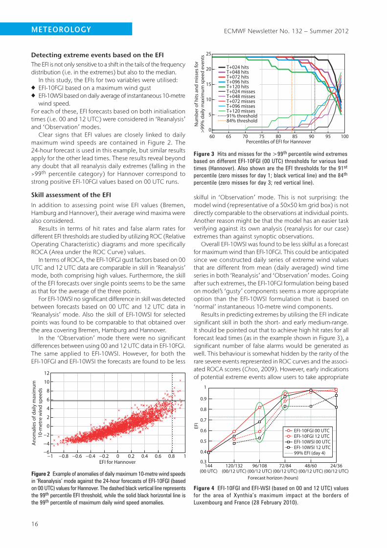
detecting extreme events based on the eFiThe EFI is not only sensitive to a shift in the tails of the frequency distribution (i.e. in the extremes) but also to the median.
In this study, the EFIs for two variables were utilised:u EFI-10FGI based on a maximum wind gustu EFI-10WSI based on daily average of instantaneous 10-metre
wind speed.For each of these, EFI forecasts based on both initialisation times (i.e. 00 and 12 UTC) were considered in ‘Reanalysis’ and ‘Observation’ modes.
Clear signs that EFI values are closely linked to daily maximum wind speeds are contained in Figure 2. The 24-hour forecast is used in this example, but similar results apply for the other lead times. These results reveal beyond any doubt that all reanalysis daily extremes (falling in the >99th percentile category) for Hannover correspond to strong positive EFI-10FGI values based on 00 UTC runs.
skill assessment of the eFi
In addition to assessing point wise EFI values (Bremen, Hamburg and Hannover), their average wind maxima were also considered.
Results in terms of hit rates and false alarm rates for different EFI thresholds are studied by utilizing ROC (Relative Operating Characteristic) diagrams and more specifically ROCA (Area under the ROC Curve) values.
In terms of ROCA, the EFI-10FGI gust factors based on 00 UTC and 12 UTC data are comparable in skill in ‘Reanalysis’ mode, both comprising high values. Furthermore, the skill of the EFI forecasts over single points seems to be the same as that for the average of the three points.
For EFI-10WSI no significant difference in skill was detected between forecasts based on 00 UTC and 12 UTC data in ‘Reanalysis’ mode. Also the skill of EFI-10WSI for selected points was found to be comparable to that obtained over the area covering Bremen, Hamburg and Hannover.
In the ‘Observation’ mode there were no significant differences between using 00 and 12 UTC data in EFI-10FGI. The same applied to EFI-10WSI. However, for both the EFI-10FGI and EFI-10WSI the forecasts are found to be less
skilful in ‘Observation’ mode. This is not surprising: the model wind (representative of a 50×50 km grid box) is not directly comparable to the observations at individual points. Another reason might be that the model has an easier task verifying against its own analysis (reanalysis for our case) extremes than against synoptic observations.
Overall EFI-10WSI was found to be less skilful as a forecast for maximum wind than EFI-10FGI. This could be anticipated since we constructed daily series of extreme wind values that are different from mean (daily averaged) wind time series in both ‘Reanalysis’ and ‘Observation’ modes. Going after such extremes, the EFI-10FGI formulation being based on model’s ‘gusty’ components seems a more appropriate option than the EFI-10WSI formulation that is based on ‘normal’ instantaneous 10-metre wind components.
Results in predicting extremes by utilising the EFI indicate significant skill in both the short- and early medium-range. It should be pointed out that to achieve high hit rates for all forecast lead times (as in the example shown in Figure 3), a significant number of false alarms would be generated as well. This behaviour is somewhat hidden by the rarity of the rare severe events represented in ROC curves and the associ-ated ROCA scores (Choo, 2009). However, early indications of potential extreme events allow users to take appropriate
meteorology
−1 −0.8 −0.6 −0.4 −0.2 0 0.2 0.4 0.6 0.8 1
−4
−6
−2
0
2
4
6
8
10
12
EFI for Hannover
Ano
mal
ies
of d
aily
max
imum
10-m
etre
win
d sp
eeds
Figure 2 Example of anomalies of daily maximum 10-metre wind speeds in ‘Reanalysis’ mode against the 24-hour forecasts of EFI-10FGI (based on 00 UTC) values for Hannover. The dashed black vertical line represents the 99th percentile EFI threshold, while the solid black horizontal line is the 99th percentile of maximum daily wind speed anomalies.
60 65 70 75 80 85 90 95 1000
5
10
15
20
25
Percentiles of EFI for Hannover
Num
ber o
f hits
and
mis
ses
for
>99
% d
aily
max
imum
spe
ed e
vent
s
T+024 hits T+048 hits T+072 hits T+096 hits T+120 hits T+024 misses T+048 missesT+072 misses T+096 misses T+120 misses 91% threshold 84% threshold
Figure 3 Hits and misses for the >99th percentile wind extremes based on different EFI-10FGI (00 UTC) thresholds for various lead times (Hannover). Also shown are the EFI thresholds for the 91st
percentile (zero misses for day 1; black vertical line) and the 84th percentile (zero misses for day 3; red vertical line).
24/36(00/12 UTC)
48/60(00/12 UTC)
72/84(00/12 UTC)
96/108(00/12 UTC)
120/132(00/12 UTC)
144(00 UTC)
0.4
0.3
0.5
0.6
0.7
0.8
0.9
1
Forecast horizon (hours)
EFI
EFI-10FGI 00 UTC EFI-10FGI 12 UTC EFI-10WSI 00 UTC EFI-10WSI 12 UTC 99% EFI (day 4)
Figure 4 EFI-10FGI and EFI-WSI (based on 00 and 12 UTC) values for the area of Xynthia’s maximum impact at the borders of Luxembourg and France (28 February 2010).

ECMWF Newsletter No. 132 – Summer 2012
17
meteorology
examples of utilising the eFiThe setting of optimal EFI thresholds is further investigated for extreme events over Hannover. All daily maximum wind speed values for Hannover (‘Reanalysis’ mode) over a period of 2,374 days are plotted in Figure 6. A selection of the four most recent spikes has been made (highlighted by a red circle). These spikes indicate the following storms: Kyrill (18 January 2007), Emma (1 March 2008), Herbert (23 March 2009) and Xynthia (1 March 2010).
As an example the various EFI-10FGI maps valid for Emma storm are displayed in Figure 7 for the forecast period from
mitigating action. Depending on their sensitivity to the event, different users will take action at different levels of risk. A user who is especially vulnerable to an extreme event may decide to act even at a relatively low risk threshold, while others may prefer to wait until the event is more certain.
setting an optimal eFi threshold
The usefulness of early indications of severe weather based on the EFI can be seen in Figure 4. This shows the EFI values for the maximum impact location (borders of Luxembourg and France) of storm Xynthia on 28 February 2010. It is clear that the EFI-10FGI is capable of providing an early indication of high winds four days in advance. The same holds for the other EFI variables but there is a delay of 24 hours.
Using the 99th percentile of EFI, very high (skilful) ROCA values were found for all three airports. This threshold is capable of providing an early indication for some extremes, but not for all (as displayed in Figure 3). By lowering this threshold, the number of hits can be increased till eventually all extremes are captured, but the number of false alarms is then increased significantly. This unavoidable drawback can be seen in Figure 5 where the number of false alarms is plotted against different EFI-10FGI thresholds for Hannover airport corresponding to the hits contained in Table 2.
The number of hits for the 24-hour forecast is equal to 9, but there are also 15 misses and 15 false alarms (Table 2). The ‘zero misses’ EFI threshold (i.e. the one corresponding to the 91st percentile), highlighted by yellow shading in Table 2, is able to predict all 24 hits (i.e. zero misses), although by doing so the number of false alarms is increased significantly and reaches 190. This limitation becomes more pronounced when different (longer) lead times are considered, as easily seen by examining the results for days 1 to 5 in Table 2. For instance, the day 5 ‘zero misses’ for the 99th percentile extreme wind anomalies corresponds to a considerably lower threshold of EFI, equal to the 70th percentile (resulting in 688 false alarms).
Overall, it is clear that all observed extremes (falling in the >99th percentile category) are linked to high positive EFI values. The highest skill in providing an early indication is from the EFI-10FGI.
9192939495969798990
20406080
100120140160180200
Percentile of EFI-FGI for Hannover
Num
ber o
f fal
se a
larm
s fo
r>
99%
dai
ly m
axim
um s
peed
eve
nts
T+024 T+048 T+072 T+096 T+120
Figure 5 Number of False Alarms for different EFI-10FGI percentile thresholds for lead times from 24 to 120 hours. It is obvious that the 91st percentile (resulting to zero misses for T+24) also introduces 190 false alarms.
EFI threshold (%) Day 1 T+24
Day 2 T+48
Day 3 T+72
Day 4 T+96
Day 5 T+120
70 24 24 24 24 24
71 24 24 24 24 23
72 24 24 24 24 23
73 24 24 24 24 23
74 24 24 24 24 23
75 24 24 24 24 23
76 24 24 24 24 23
77 24 24 24 24 23
78 24 24 24 24 21
79 24 24 24 24 21
80 24 24 24 23 20
81 24 24 24 23 20
82 24 24 24 23 20
83 24 23 24 23 20
84 24 23 24 23 19
85 24 23 23 23 19
86 24 23 23 23 19
87 24 23 22 21 19
88 24 23 22 21 19
89 24 23 22 19 19
90 24 21 22 19 19
91 24 20 21 19 18
92 23 20 20 17 16
93 23 20 18 16 16
94 23 19 17 15 16
95 23 19 15 14 13
96 21 16 12 14 12
97 18 14 12 14 10
98 13 12 10 12 8
99 9 8 6 7 5
Table 2 Number of Hits for >99th percentile extremes based on various EFI-10FGI (00 UTC) thresholds for different lead times valid for Hannover (maximum number of hits: 24). The red cells indicate the ‘zero misses’ EFI thresholds for the various lead times.

18
ECMWF Newsletter No. 132 – Summer 2012meteorology
24 to 132 hours with 12-hour intervals. It is clear that both the 95% and 98% EFI thresholds (highlighted by a yellow line) are able to provide an early indication of the Emma windstorm from day 5.5 (T+132 h) onwards.
To investigate whether these thresholds can provide an early indication of the other storms considered here, Figure 8 is constructed. Clearly both the 95th and 98th percentile thresholds work quite well for the Kyrill and Emma storms, but they seem to be inadequate for Herbert and Xynthia. More specifically, for Herbert, using the 98th percentile threshold fails to give an indication of high winds, while use of the 95th percentile seems to do a better job for lead times shorter than 84 hours. As for Xynthia, the 98th percentile seems to work only for the 96-hour lead time, while the 95th percentile threshold works for all lead times shorter than 120 hours (except for the 36-hour one). For both Herbert and Xynthia, a slightly lower threshold (say between 90th and 95th) could have resulted in forecasters having an early indication of the severity of the winds associated with the approaching storms.
0 500 1000 200015000
2
4
6
8
10
12
14
16
18
Days (1 December 2003 to 31 May 2010)
Win
d sp
eeds
(m/s
)
Kyrill storm18 January 2007
Emma storm1 March 2008
Herbert storm23 March 2009
Xynthia storm1 March 2010
EPS t+(0–24h)EPS t+(12–36h)EPS t+(24–48h)EPS t+(36–60h)EPS t+(48–72h)EPS t+(60–84h)EPS t+(72–96h)
EPS t+(84–108h)EPS t+(96–120h)
EPS t+(108–132h)–100% –50% EFI 50% 100%
Extreme Forecast Index for Emma Stormvalid for 3 March 2008 over Hannover
93%95%95%92%94%95%95%92%93%90%
Figure 6 Time series of daily maximum wind speed values for Hannover over a period of 2,374 days from 1 December 2003 to 31 May 2010 (‘Reanalysis’ mode).
Figure 7 Example of different EFI-10FGI maps (‘EFI-GRAM’) valid for the Emma storm hitting Hannover airport on 1 March 2008. The arrows from each map (initiating from Hannover’s position) point to the part of the central graph constituting the currently operational ‘EFI-GRAM’. The different forecast steps are displayed on the left of the diagram while the exact EFI values over Hannover are displayed on the right. Forecast lead times span from 24 to 132 hours with 12-hour intervals. A near-crash incident of an Airbus A320 took place at the nearby Hamburg airport.

19
ECMWF Newsletter No. 132 – Summer 2012 meteorology
overviewThis study is focused on the early indication of extreme winds in the short- and early medium-range using the EFI. For the assessment of the quality of the EFI, three synoptic stations at airports in North Germany (i.e. Bremen, Hamburg and Hannover) were considered. An investigation of synop-tic weather type for each station indicated that all wind extremes (exceeding the 99th percentile) were linked to surface pressure lows being advected in south-westerly and north-westerly flow regimes.
For the objective evaluation of early indications of an extreme weather event, the EFI for wind gusts and mean
wind speed were compared to daily maximum wind speeds (in both ‘Reanalysis’ and ‘Observation’ modes). The highest skill in detecting extremes is given by the EFI-10FGI. Extreme observed events are clearly linked to higher values of the EFI.
Although the EFI is designed to be used qualitatively as a general ‘alarm bell’ for potential extreme weather, it is also possible to use the EFI in a more quantitative way. The user can select a specific EFI threshold and take appropriate action whenever the EFI exceeds this threshold. The examples shown in this article illustrate some possible uses of this objective approach. There is no direct mathematical correspondence between percentiles of the EFI distribution and those of the climate distribution. However, in general selecting a high EFI threshold (e.g. the 99th percentile) focuses on the strongest warnings and will have fewest false alarms.
By lowering this threshold the number of hits is increased until all extremes are captured (i.e. zero misses), but by doing so the number of false alarms is increased significantly. Some users will be especially sensitive to missed events while others will be interested in limiting the number of false alarms. As this study has shown, each user is able to choose an appropri-ate EFI threshold for their own requirements, to provide an optimal trade-off between hits and false alarms.
FUrtHer readingandersson, e. & d. richardson, 2011: Forecast performance 2011. ECMWF Newsletter No. 130, 15–16.Bissolli, P. & e. dittmann, 2001: The objective weather type classification of the German Weather Service and its possibilities of application to environmental and meteorological investigations. Meteorologische Zeitung, 10, S. 253–260.Bougeault, P., 2003: WGNE survey of verification methods for numerical prediction of weather elements and severe weather events. Report 18 CAS/JSC WGNE.Choo, C.w., 2009: Information use and early warning effectiveness: Perspectives and prospects. J. Am. Soc. Information Sci. Technol., 60, 1071–1082.donat, m.g., 2010: European wind storms, related loss potentials and changes in multi-model climate simulations. Doktorarbeit am Institut für Meteorologie, Freie Universität Berlin, 175 pp.lalaurette, F., 2003: Early detection of abnormal weather using a probabilistic Extreme Forecast Index. Q.J.R. Meteorol. Soc., 129, 3037–3057.lalaurette, F. & g. v.d. grijn, 2005: Predictability of Weather and Climate: Ensemble forecasts: can they provide useful early warnings? In Predictability of Weather and Climate, Palmer, T.N. and R. Hagedorn, editors, Cambridge University Press.murphy, a.H., 1991: Probabilities, odds and forecasts of rare events. Wea. Forecasting, 6, 302–307.richardson, d.s., J. Bidlot, l. Ferranti, a. ghelli, t. Haiden, t. Hewson, m. Janousek, F. Prates & F. Vitart, 2011: Verification statistics and evaluations of ECMWF forecasts in 2010-2011. ECMWF Tech. Memo. No. 654.simmons, a., s. Uppala, d. dee & s. Kobayashi, 2007: ERA-Interim: New ECMWF reanalysis products from 1989 onwards. ECMWF Newsletter No. 110, 25–35.
93%88%88%85%83%87%86%85%82%83%
a KyrillEPS t+(0–24h)
EPS t+(12–36h)EPS t+(24–48h)EPS t+(36–60h)EPS t+(48–72h)EPS t+(60–84h)EPS t+(72–96h)
EPS t+(84–108h)EPS t+(96–120h)
EPS t+(108–132h)–100% –50% EFI 50% 100%
b Emma93%95%95%92%94%95%95%92%93%90%
EPS t+(0–24h)EPS t+(12–36h)EPS t+(24–48h)EPS t+(36–60h)EPS t+(48–72h)EPS t+(60–84h)EPS t+(72–96h)
EPS t+(84–108h)EPS t+(96–120h)
EPS t+(108–132h)–100% –50% EFI 50% 100%
d Xynthia68%63%65%68%70%62%78%61%33%18%
EPS t+(0–24h)EPS t+(12–36h)EPS t+(24–48h)EPS t+(36–60h)EPS t+(48–72h)EPS t+(60–84h)EPS t+(72–96h)
EPS t+(84–108h)EPS t+(96–120h)
EPS t+(108–132h)–100% –50% EFI 50% 100%
c Herbert74%68%67%65%65%58%69%54%53%53%
EPS t+(0–24h)EPS t+(12–36h)EPS t+(24–48h)EPS t+(36–60h)EPS t+(48–72h)EPS t+(60–84h)EPS t+(72–96h)
EPS t+(84–108h)EPS t+(96–120h)
EPS t+(108–132h)–100% –50% EFI 50% 100%
Figure 8 EFI-10FGI values over Hannover for four windstorms (a) Kyrill (18 January 2007), (b) Emma (1 March 2008), (c) Herbert (23 March 2009) and (d) Xynthia (1 March 2010). The 95th and 98th percentile thresholds are plotted using a yellow line.

ECMWF Newsletter No. 132 – Summer 2012
20
meteorology
Towards an operational GMES Atmosphere Monitoring Service
VINCENT-HENRI PEUCH, RICHARD ENGELEN
The MACC-II (Monitoring Atmospheric Composition and Climate - Interim Implementation) project delivers the pre-operational atmospheric composition services
of GMES (Global Monitoring for Environment and Security, http://www.gmes.info) and strengthen the production chains in order to be in readiness for the operational phase, due to start immediately after the end of the project. MAC-II succeeded the MACC project (see ECMWF Newsletter No. 123, 10–13) at the end of 2011 and will run till July 2014. It is funded under the European Union’s Seventh Framework Programme as was MACC.
This article provides some insight in the global production chain of MACC-II, focusing on reactive gases, aerosol and then greenhouse gases. These aspects share commonalities for the preparation of the operational phase, but have different level of maturity and face specific scientific and technical challenges. We highlight also that the developments on atmospheric composition performed in the context of MACC-II are also very promising from the point of view of improving numerical weather prediction (NWP) and existing ECMWF products. The vision of ECMWF, supported by its Member States, that atmospheric composition would not only extend the scope of useful products connected with meteorology at large but would also benefit weather forecasts is becoming a reality. Visionary? Maybe not quite so.
“The chemical composition of air, the nature of the particles it transports, provides also its own piece of information. One never has enough enlightening in solving such a difficult and important problem as weather forecasting”
H. Marié-Davy (Les mouvements de l’atmosphère et les variations du temps, Masson, Paris, 1877)
Background to gmes and maCC-ii
The purpose of GMES is to deliver information about envi-ronment and security based on Earth-monitoring data collected from space, air, water or land. The GMES services deal with six areas: marine, atmosphere, land, emergency, security, and climate change.
There are currently discussions at the European level on the sustainable funding scheme for GMES, either through a budget line in the Multi-annual Financial Framework (the main budget of the European Union, EU) or a dedicated intergov-ernmental fund. However, the full development of GMES, including the space, in-situ and services components, is expected to go forward with the strong backing of cost-benefit analyses (Pricewaterhouse-Coopers, 2006; booz&co., 2011). Return on investment ratios of 4 to 10 make GMES an integral
part of a successful implementation of the Lisbon strategy of the EU which is concerned with developing a competitive and dynamic knowledge-based economy. But beyond economic aspects, GMES will provide information of unprec-edented quality on the environment at large, as well as support European policies on emergencies and security.
MACC-II follows in the track of previous European projects, MACC and GEMS, to deliver information services on atmos-pheric composition: reactive gases, aerosol, greenhouse gases, European air quality, and solar and ultra-violet radiation. As with its predecessor projects, MACC-II is co-ordinated by ECMWF. It involves a large consortium of 36 partners from 13 countries. Nine National Weather Services (AEMET, DWD, FMI, IM, KNMI, met.no, Météo-France, Met Office and SMHI), as well as a number of National Environment Agencies and academic partners, constitute the bulk of the consortium. The website of MACC-II, http://www.gmes-atmosphere.eu, delivers the portfolio of products in the form of graphics and maps, and also serves as a gateway for access to numerical data.
As in MACC, there are two main production chains: a global one, operated at ECMWF, and a regional one, operated by a network of seven processing centres federated by Météo-France, and delivering European scale air quality services. Most services are forecasts for a few days ahead and delivered in near-real-time, but some of them are also delivered in delayed mode – a few months after time – as this is necessary to acquire the observations, particularly for greenhouse gases.
The MACC project produced a new ‘chemical’ reanalysis of the period 2003–2010, which supersedes the GEMS one and is now being extended for the years 2011 and 2012 as part of MACC-II. The number of users of this MACC reanalysis is already in excess of six hundred, covering most countries in the world (Figure 1).
Value of comprehensive atmospheric chemistry representation in the iFs
GEMS and MACC have put significant resources into the building of a coupled chemical data assimilation system that
Figure 1 Countries with users of MACC reanalysis data for 2003–2011 are marked in blue (as of May 2012).

ECMWF Newsletter No. 132 – Summer 2012
21
meteorology
allows assimilating satellite data of O3, CO, NO2, and SO2 in the IFS while properly accounting for the full underlying chemistry.
Validation of the MACC reanalysisThe MACC reanalysis, already mentioned, was the occasion to evaluate the skill of the main system used: Integrated Forecasting System (IFS) at a T255 reduced Gaussian grid (approximately 80 km horizontal resolution) resolution and 60 levels, coupled to the Chemistry and Transport Model (CTM) MOZART-3 using the OASIS4 coupling software (Valcke & Redler, 2006). This system allows representation of 115 chemical compounds, offering thus a reasonably comprehensive description of atmospheric chemistry.A detailed report is available on the validation of the reanalysis (Inness et al., 2012, ECMWF Tech. Memo. No. 671). Figure 2 highlights one of the results: it is a comparison of ozone profiles at Alert, Canada (82.5°N, 62.3°W, the northernmost permanently inhabited place in the world, only 500 miles from the North Pole) for the MACC reanalysis and for the ERA-Interim reanalysis against ozone sondes for the period 2003 to 2010. The performance of the MACC reanalysis is strikingly better than ERA-Interim regarding tropospheric ozone: errors with the MACC system range between ±30%, while errors reach 100% in ERA-Interim and show marked seasonal variations. This is not unex-pected, as the representation of ozone in ECMWF operations and ERA-Interim only accounts for (simplified) stratospheric ozone chemistry, while MACC has a representation of the
complex non-linear tropospheric ozone formation from its precursors, nitrogen oxides and volatile organic compounds. The MACC system also allows a better use of the available satellite data with sensitivity to ozone in the troposphere. In the stratosphere the skill of both the MACC reanalysis and ERA-Interim is much better than in the troposphere (±10%), with the MACC reanalysis also being marginally more realistic than ERA-Interim at these altitudes.
The good quality of the MACC ozone reanalysis is not only important for users interested in the full vertical profile of ozone: in the MACC system there are much better pros-pects for using the actual ozone fields in the computation of radiation as well as in the assimilation of radiances that are sensitive to ozone. A first step has been to use climatolo-gies of key radiative species from the MACC reanalyses in the IFS as a default. Also, Engelen & Bauer (2011) have shown the benefit of using MACC’s CO2, rather than a fixed back-ground value, in reducing the bias correction needed for assimilation of IASI and AIRS radiances. Making the MACC-II suite operational will also offer the opportunity to use time-dependent forecast fields, which is a very promising path for weather prediction, considering in particular the sensitiv-ity of surface temperature to ozone content in the upper troposphere/lower stratosphere region.
In-line representation of atmospheric chemistry in IFSAnother objective of MACC-II is to be in a position to operate, at the end of the project, a validated version of the IFS augmented with a comprehensive in-line representation of atmospheric chemistry and associated processes, called C-IFS hereafter (Flemming et al., 2009) – a modelling and data assimilation system with little or no equivalent worldwide. C-IFS will replace the current systems based on coupled models, offering increased computational efficiency as well as the option to activate feedback of composition on physical processes at each model time step.Figure 3 illustrate the capabilities of the MACC-II system, by presenting a map of carbon monoxide (CO), a pollutant emitted by incomplete combustion processes of human (e.g. car traffic, industries, residential heating, energy production) and natural (e.g. wildfires and biomass burning) origins. CO has an atmospheric lifetime of approximately one month. It is represented here with a simplified version of C-IFS, comprising a linear representation of CO chemistry. C-IFS can be run at much higher resolution than the current MACC systems.
Figure 3 shows a zoom over Europe of travelling CO plumes. This is of direct interest for applications such as regional air-quality forecasting, which can now include the effects of long-range transport of pollutants, but it is opening interesting perspectives for NWP as well. CO is one of the tropospheric species which are best observed from space, due to its absorption properties in the short-wave and thermal infra-red, and instruments such as TERRA/MOPITT (NASA) and MetOp/IASI currently provide good monitoring capabili-ties. The use of the quasi-tracer properties of CO could help improve winds (especially in cloud free areas, where cloud-drift winds cannot be used by design) using data assimilation,
5
a MACC reanalysis
2003 2004 2005 2006 2007 2008 2009 2010
–100–80 –60 –40 –20 0 20 40 60 80 100
10
20
50
Pres
sure
(hPa
)
100
200
500
1000
5
b ERA-Interim
2003 2004 2005 2006 2007 2008 2009 2010
10
20
50
Pres
sure
(hPa
)
100
200
500
1000
Figure 2 Verification of ozone profiles against ozone sondes at Alert (Canada) for (a) MACC reanalysis and (b) ERA-Interim (bottom) in percent.

ECMWF Newsletter No. 132 – Summer 2012
22
meteorology
in a similar manner as it at been shown successful for ozone and winds in the upper troposphere/lower stratosphere.
C-IFS will initially include three state-of the-art chemical schemes: TM5 (from KNMI), MOCAGE (from Météo-France) and MOZART-3 (from NCAR, USA, and Research Centre Jülich). However, part of the MACC-II plan is to release C-IFS as a community model, following directly in the steps of open-IFS for the meteorological part. This will allow a wider range of partners to include their chemical parametrizations in C-IFS – for the benefit of research activities and to improve the GMES atmospheric services delivered to users.
Forecasting dust, smoke and other aerosol
Contrary to the path chosen for reactive gases, which neces-sarily involves addition of the order of 100 tracers or more to represent complex non-linear chemical processes in the troposphere, aerosol representation has been directly introduced in-line in the IFS since the GEMS project. The initial ‘compact’ representation of aerosol in the IFS model-ling and assimilation suite has already been the topic of articles in the winter 2007/08, summer 2008 and spring 2009 editions of the ECMWF Newsletter. Since then, devel-opments have carried on both internally at ECWMF, especially to improve incrementally the representation of dust and volcanic ash, and externally to test a much more detailed representation of tropospheric (University of Leeds, UK, based on the GLOMAP model) and stratospheric (LATMOS, France, based on the REPROBUS model) aerosols. Integration of these advanced modules is on-going during MACC-II and the evaluation of relative performance will guide the next steps towards operational use.
Aerosol assimilation/forecasting systemAlready, the new version of the aerosol scheme implemented in May 2012 produced a significant improvement in the skill of products, both analyses and forecasts. This is illustrated by Figure 4 showing the mean bias of the aerosol optical depth (AOD) relative to observations from the AERONET network (Holben et al., 1998) as a function of forecast lead time (panel a) and day of the month (panel b).
Global aerosol products have been among the most widely used in MACC and MACC-II. Support to Volcanic
Ash Advisory Centres during volcanic eruptions has already been documented (e.g. ECMWF Newsletter No. 123, 9). Aerosols affect visibility and radiation, and thus are of significant interest for meteorological forecasters in ECMWF Member States. GEMS and MACC have allowed develop-ment of one of the more advanced aerosol assimilation and forecasting systems, and ECMWF is now playing an impor-tant role in international initiatives such as the International Cooperative for Aerosol Prediction (Benedetti et al., 2011).
Long-range transport of natural aerosolsThe interaction with users in MACC and MACC-II, particularly in the air quality policy sector, has confirmed a major interest of these communities for accurate estimates of long-range transported natural aerosol, in particular soil dust and aerosol from large wildfires. Indeed, European Directives require EU Member States to take action when the PM10 (particulate matter of diameter smaller than 10 µm) regulatory threshold is exceeded. Local sources in general dominate, but the contribution of remote sources can be significant for some exceptional events.
In a meeting in May 2011, the European Commission confirmed interest on its behalf and of its Member States for natural aerosol estimates from MACC-II and, later, the GMES atmospheric service as an input to the air quality reporting process. Figure 5 provides an example of very high surface PM10 measured in Virolati (Finland) as a consequence of the Russian fire events of July and early August 2010. In real-time, the MACC system predicted that
3000ppb
200010005002001801601401201008060400
Figure 3 Example of surface CO distribution at high resolution over Europe using linear CO as part of C-IFS developments.
a Forecast lead time
b Day of the month
0.05
0
–0.05
–0.1
–0.15
–0.2
–0.25
0.05
0
–0.05
–0.1
–0.15
–0.2
–0.25
0 6 12 18 24 30 36 42 48Forecast lead time (hours)
54 60 66 72 78 84 90 96
4 6 8 10 12 14 16 18 20May JuneDay in 2012
Mea
n b
ias
of A
OD
Mea
n b
ias
of A
OD
22 24 26 28 31 1 3
New schemeOld scheme
Figure 4 Verification of the aerosol forecasts for the new and old aerosol representation in MACC/IFS in terms of the mean bias of the aerosol optical depth (AOD) relative to observations from the AERONET network as a function of (a) forecast lead time and (b) day of the month for May 2012.

ECMWF Newsletter No. 132 – Summer 2012
23
meteorology
only Southern Finland out of the 27 EU countries would be significantly affected by the transport of fire aerosol from the sources near Moscow; this was useful information, in particular for the European Environmental Agency (EEA).
Figure 5 shows that the skill of the system is due both to the assimilation of aerosol optical depth data (in this case from the MODIS sensors on board the Terra and Aqua satellites), allowing to capture the travelling plumes of pollutants, and to the prescription of fire sources depending on satellite-detected ‘Fire Radiative Power’ (FRP, also a MODIS product) of the actual fires (Kaiser et al., 2011). A system based on climatological fire emissions and no data assimilation completely fails, as expected, to predict the observed extreme levels observed in Virolati (Finland) in excess of 100 µg m–3.
Benefits of including aerosols for NWPThe inclusion of aerosols in atmospheric models has a large potential to improve NWP forecasts. Aerosol effects on cloudiness and the hydrological cycle are the topic of acute scientific debate, in particular concerning the indirect effects. Initial tests at ECMWF indicate that, though neutral overall on main global skill scores, taking into account the
August 2010
Surface observationsFull MACC II
Degraded MACC II
87654 9 10 11
140
120
100
80
60
Conc
entr
atio
n of
PM
10 (µ
g/m
-3)
40
20
0
Figure 5 Concentrations of PM10 (see text) at Virolati, Southern Finland, during the period 4–11 August caused by the Russian fires near Moscow. Surface observations are black dots and the lines represent the full MACC-II system (blue) and two degraded versions: no assimilation and FRP-based ‘dynamical’ fire emissions (green) and no assimilation and climatological fire emissions (yellow).
extending headline skill scores for atmospheric composition
Headline Skill Scores (HSS) have been defined to monitor progress over time of ECMWF’s main products and imple-mentation of our strategy. These skill scores use long-standing and widely recognised metrics for skill forecasts (anomaly correlation at 500 hPa) as well as a range of additional indicators specifically suited for follow-ing up the forecast skill on extreme events, as well as the EPS products at the different time horizons.With the approaching operational phase of GMES atmos-phere, it has been decided to look into the extension of HSS into atmospheric composition. Though MACC-II has a very comprehensive validation sub-project looking in detail at all aspects of our products, making use as far as possible of independent satellite and in-situ composition data, the definition of HSS is a specific target to reflect overall performance of the global atmospheric composi-tion system operated at ECMWF by only a few synthetic indicators. The ‘chemical’ HSS will comprise four indicators to sample the main aspects of the system:u Vertical ozone profile (as a proxy for stratospheric
composition)u Surface carbon monoxide (as a representative of tropo-
spheric chemistry and of boundary conditions used for air quality application)
u Aerosol optical depth (AOD)u Surface in-situ CO2 and CH4
We illustrate here the indicator for the skill of the ozone profile. It is based upon a figure of merit (a quantity char-acterising the performance of a system relative to its alternatives) comparing the modelled profile (forecast, analysis or reanalysis) with an observed profile from an
independent ozone sonde, a perfect match of the two being 1. This unique indicator captures not only differences in the vertically integrated content of ozone (total column), but also if there are issues with the vertical structure of the modelled profile – which could be due to dynamical and/or chemical processes.
Though in principle this skill score can be computed for any ozone sonde regular launch site, we have selected Neumayer in Antarctica, which witnesses in particular the representation of dynamical and chemical processes associated with the ozone hole. The figure shows that the MACC near-real-time main product (three successive system evolutions) has clearly outperformed the skill of ECMWF operational ozone, while improving over the first year of routine production.
MACC product
Operations
Aug2008
Dec Apr2009
Aug Dec Apr2010
Figu
re o
f mer
it
Aug Dec Apr2011
Aug Dec Apr2012
0.6
0.7
0.8
0.9
1
Skill of ozone profile. Figure of merit for monthly-mean profiles of ozone over Neumayer (Antarctica) from August 2008 to May 2012.
a

ECMWF Newsletter No. 132 – Summer 2012
24
meteorology
direct effect of aerosols brings local/regional benefits – these can be marked during strong episodes such as large dust outbreaks. It is less the load of aerosol than its physical properties, size distribution and spatio-temporal variability that matters really and in-line integration in the IFS makes it possible to be a pioneer in this direction.
monitoring methane and carbon dioxide
While the global MACC-II system generally has been focus-ing on assimilating satellite observations, different solutions had to be found for the greenhouse gases due to a lack of accurate satellite observations for carbon dioxide (CO2) and methane (CH4).
Observations of greenhouse gases from spaceThe SCIAMACHY instrument has provided a long record of methane observations, but the recent loss of the ENVISAT satellite has ended this time series. The European IASI and Japanese GOSAT instruments also provide information on methane, but their retrieval algorithms are not yet fully mature.
For CO2 the situation is even more problematic with the AIRS and IASI instruments providing some information about the global growth rate of CO2 but without any significant regional information. Retrieval algorithms for the Japanese GOSAT instrument are not mature enough to fully constrain atmospheric CO2 concentrations and surface fluxes.
MACC-II greenhouse gas products
This situation has forced the MACC-II project to explore other directions to provide useful greenhouse gas services resulting in three main products.u Fluxes of CO2 and CH4 using flux inversion. Estimation
of surface fluxes from atmospheric concentration obser-vations remains a key component of MACC-II. These flux inversions are provided by our partners LSCE (Laboratoire des Sciences du Climat et l’Environnement) and JRC (European Commission’s Joint Research Centre) for CO2 and CH4, respectively. For CO2, the flux inver-sions are currently based on surface flask observations only, but trials with the slowly-maturing GOSAT retriev-als are starting to look promising. For CH4, the flux inversions were based on a combination of surface flask observations and SCIAMACHY retrievals. With the loss of ENVISAT, a transition to the use of GOSAT retrievals is currently under way.
u Fields of CO2 and CH4 using fluxes from flux inversion. The optimized fluxes from the flux inversions are used in the IFS model to produce atmospheric CO2 and CH4 fields at relatively high resolution (currently T255L60). Validation has shown that these atmospheric concentra-tions are quite realistic and therefore very useful to produce boundary conditions for regional greenhouse gas models or to test new satellite retrieval data, such as from GOSAT or the upcoming Sentinel-5p satellite.
u Fields of CO2 using fluxes from C-TESSEL. The above two products are produced in delayed (six months to one year behind near-real-time) and reanalysis modes because of the very limited availability of surface observations and greenhouse gas satellite data in near-real-time. Therefore, the third product makes use of the land-surface modelling developments at ECMWF. The work in the MACC-II and GEOLAND2 projects at ECMWF has been very collabora-tive on the development and use of the C-TESSEL land carbon model. With the implementation of the C-TESSEL model in the IFS, CO2 fluxes can be modelled on-line allowing a realistic forecast capability for the MACC-II CO2 system. Observations are used to regularly update some key C-TESSEL model parameters as well as to constrain the global CO2 growth rate providing reasonably accurate forecasts of CO2 that can be used for boundary conditions, flight campaign planning, and near-real-time monitoring and processing of satellite data.
Figure 6 shows the validation of modelled CO2 using fluxes from flux inversion (panel b) and C-TESSEL (panel c) against observations from GLOBALVIEW-CO2 (2011) (panel a) as a function of time and latitude. While some differences between the observations and the model runs remain, it is clear that the main variability of CO2 is well-captured, which is confirmed by other independent observations as well.
looking ahead
Based on GEMS and MACC, MACC-II delivers a wide range of services on atmospheric composition. As a result, its user base is growing and MACC-II is attracting worldwide atten-tion both on the products available and on the associated
Contribution to the annual report on the state of the Climate
MACC and now MACC-II is a regular contributor to the annual supplement of the Bulletin of the American Meteorological Society on the ‘State of the Climate’. Anomalies in emissions due to biomass burning and in aerosol distributions (distinguishing between sea salt, dust, biomass burning and sulphate components) are provided to this international reference publication, which aims at regrouping best accurate estimates on the different component of the Earth’s climate system.
-0.5 -0.1 -0.08 -0.06 -0.04 -0.02 0.02 0.04 0.06 0.08 0.1 0.5
Example of MACC information included in ‘State of the Climate’ report. Anomolous distribution of carbonaceous aero-sol optical depth for September to November 2011 with respect to MACC reanalysis average (2003–2010) indicating a quiet season in South America and a highly active season in Australia.
b

ECMWF Newsletter No. 132 – Summer 2012
25
meteorology
research conducted at ECMWF and at partners’ organisa-tions. While MACC-II is consolidating the production chains in preparation of the GMES operational phase in the second half of 2014, there are significant challenges ahead such as making the move to an in-line representation of chemistry in the IFS or evolving towards a more detailed aerosol representation that is linked with clouds and precipitation. Finally, MACC-II has begun to illustrate how atmospheric composition developments can benefit NWP and the meteorological reanalysis by developing the IFS in such a way that the representation of Earth-system processes are more integrated and comprehensive.
FUrtHer readingBenedetti, a., J.-J. morcrette, o. Boucher, a. dethof, r.J. engelen, m. Fisher, H. Flentje, n. Huneeus, l. Jones, J.w. Kaiser, s. Kinne, a. mangold, m. razinger, a.J. simmons, m. suttie & the gems aer team, 2008: Aerosol analysis and forecast in the European Centre for Medium-Range Weather Forecasts Integrated Forecast System: Data Assimilation. J. Geophys. Res., D13205, 114, doi:10.1020/2008JD011115.Benedetti, a., J.s. reid & P.r. Colarco, 2011: International Cooperative for Aerosol Prediction Workshop on Aerosol Forecast Verification. Bull. Am. Meteorol. Soc., 92, ES48–ES53.booz&co., 2011: Cost-Benefit Analysis for GEMS, European Commission: Directorate-General for Enterprise and Industry. London, 19 September 2011,http://ec.europa.eu/enterprise/policies/space/files/gmes/studies/ec_gmes_cba_final_en.pdf.engelen, r.J. & P. Bauer, 2011: The use of variable CO2 in the data assimilation of AIRS and IASI radiances. Q. J. R. Meteorol. Soc., doi: 10.1002/qj.919Flemming, J., a. inness, H. Flentje, V. Huijnen, P. moinat, m.g. schultz & o. stein, 2009: Coupling global chemistry
transport models to ECMWF’s integrated forecast system, Geosci. Model Dev., 2, 253–265, doi:10.5194/gmd-2-253-2009.gloBalView-Co2, 2011: Cooperative Atmospheric Data Integration Project – Carbon Dioxide, CD-ROM, NOAA ESRL, Boulder, Colorado [Also available on Internet via anonymous FTP to ftp.cmdl.noaa.gov, Path: ccg/co2/GLOBALVIEW].Holben, B.n., t.F. eck, i. slutsker, d. tanré, J.P. Buis, a. setzer, e. Vermote, J.a. reagan, y.J. Kaufman, t. nakajima, F. lavenu, i. Jankowiak & a. smirnov, 1998: An emerging ground-based aerosol climatology: Aerosol optical depth from AERONET. J. Geophys. Res., 103d, 12067–12097.inness, a., F. Baier, a. Benedetti, i. Bouarar, s. Chabrillat, H. Clark, C. Clerbaux, P. Coheur, r.J. engelen, Q. errera, J. Flemming, m. george, C. granier, J. Hadji-lazaro, V. Huijnen, d. Hurtmans, l. Jones, J.w. Kaiser, J. Kapsomenakis, K. lefever, J. leitão, m. razinger, a. richter, m.g. schultz, a.J. simmons, m. suttie, o. stein, V. thouret, m. Vrekoussis, C. Zerefos & the maCC team, 2012: The MACC reanalysis: An 8-year data set of atmospheric composition. ECMWF Tech. Memo. No. 671.Kaiser, J.w., a. Heil, m.o. andreae, a. Benedetti, n. Chubarova, l. Jones, J.-J. morcrette, m. razinger, m.g. schultz, m. suttie & g.r. van der werf, 2012: Biomass burning emissions estimated with a global fire assimilation system based on observed fire radiative power. Biogeosciences, 9, 527–554.Pricewaterhouse-Coopers, 2006: Main Report Socio-Economic Benefits Analysis of GMES, European Space Agency Contract Number 18868/05, October 2006,http://esamultimedia.esa.int/docs/GMES 261006_GMES_D10_final.pdfValcke, s. & r. redler, 2006: OASIS4 User Guide (OASIS4\_0\_2). PRISM–Support Initiative, Technical Report No 4. Available fromhttp://www.prism.enes.org/Publications/index.php.
398 ppm395392389386383380
J F M A M J J A S O N D
90
60
30
0
–30
–60
–90
a Observed
J F M A M J J A S O N D
90
60
30
0
–30
–60
–90J F M A M J J A S O N D
90
60
30
0
–30
–60
–90
c Using C-TESSELb Using �ux inversion
Figure 6 Validation of modelled CO2 against observations: (a) the processed marine boundary layer surface flask observations from GLOBALVIEW-CO2, (b) the results using optimized fluxes from a flux inversion, and (c) the results using C-TESSEL CO2 fluxes.
ECMWF Newsletter No. 132 – Summer 2012
26
meteorology
Blending information from infrared radiances with ultraviolet data in the operational ozone analysis
ROSSANA DRAGANI, TONy MCNALLy
On 15 November 2011, ECMWF implemented the operational assimilation of ozone-sensitive infrared (IR/O3 hereafter) radiances from three sounders,
namely AIRS, IASI and HIRS (acronyms and abbreviations not defined in the text are listed in Table 1). This represents a major milestone in exploiting infrared sounders and analysing ozone.
In the past, NWP systems have relied operationally upon ozone products retrieved from BUV (Backscatter Ultra Violet) sensors, such as SBUV (Solar Backscatter Ultra Violet), and TOMS (Total Ozone Mapping Spectrometer) to constrain the analysis of ozone. However, a limitation of this data is that it requires sunlight and this leaves half of the globe unobserved daily. Also at high latitudes very few observa-tions can be used throughout the entire winter season. A further limitation of BUV data is that, while it has good sensitivity to ozone near the altitude of maximum concentra-tion (approximately 10–20 hPa), it is almost blind to important ozone variations at lower levels (e.g. in the upper troposphere and lower stratosphere).
Given the obvious limitations of BUV data, a number of studies have demonstrated that substantial improvements can be achieved by assimilating ozone profiles retrieved from limb-viewing infrared (IR) or microwave (MW) instru-ments (such as MIPAS or MLS) that have been carried as demonstration missions on research satellites. These sensors successfully operate in the absence of sunlight and provide (by virtue of their limb-viewing geometry) highly-detailed vertical information on the ozone concentration from the upper troposphere to the upper stratosphere. However, this data cannot be regarded as a long-term solution for operational NWP as at present there are no definite plans to deploy any limb-viewing ozone-sensitive instruments (either MW or IR) in the foreseeable future.
For this reason the exploitation of IR/O3 radiances meas-ured by nadir viewing sensors on operational satellites (such as IASI and HIRS) represents an appealing and arguably necessary supplement to the established BUV data. While nadir sounding IR/O3 observations cannot offer detailed vertical information on ozone, they do provide comple-mentary sensitivity to the ozone concentration at lower levels in the atmosphere (mostly the upper troposphere) and they have no sampling restrictions related to the pres-ence of sunlight. The operational provision of these sensors is guaranteed for the foreseeable future and there is an
extensive historical archive of data to support climate reanalysis studies.
Han & McNally (2010) (Han & McNally hereafter) presented an initial assessment of the potential impact of assimilating IR/O3 radiances from IASI within a simplified version of the ECMWF system. Their study compared inde-pendent, unassimilated MLS ozone retrievals with the ozone analyses obtained from three experiments:u Baseline, with no assimilated ozone data.u Control in which only BUV ozone products were
assimilated.u Experiment that used only IASI IR/O3 radiances.
Results showed that, with respect to the baseline, the assimilation of IASI IR/O3 radiances could significantly improve the fit of the ozone analyses to the independent MLS ozone profiles. Indeed, in some areas the fit was
Instruments
AIRS Advanced InfraRed Sounder
GOME-2 Second generation Global Ozone Monitoring Experiment
HIRS High-resolution Infrared Radiation Sounder
IASI Infrared Atmospheric Sounding Interferometer
MIPAS Michelson Interferometer for Passive Atmospheric Sounding
MLS Microwave Limb Sounder
OMI Ozone Monitoring Instrument
SCIAMACHY Scanning Imaging Absorption Spectrometer for Atmospheric Chartography
SEVIRI Spinning Enhanced Visible Infra-Red Imager
Satellites
ENVISAT Environmental Satellite
MetOp-A Meteorological Operational Satellite-A
MSG Meteosat Second Generation
Space agencies
ESA European Space Agency
EUMETSAT European Organisation for the Exploitation of Meteorological Satellites
NASA National Aeronautics and Space Administration
NOAA National Oceanic and Atmospheric Administration
Table 1 Acronyms and abbreviations not defined in the text.

ECMWF Newsletter No. 132 – Summer 2012
27
meteorology
comparable or better than that obtained from the BUV data. Han & McNally showed that the IR/O3 radiances are most sensitive in the upper troposphere – lower stratosphere region, as opposed to the BUV data that can constrain the ozone field in the middle stratosphere. This would suggest that the two data types (IR and BUV) could be used syner-gistically and provide complementary information to the ozone assimilation system. This article documents the efforts to establish an optimal blend of these two very different sources of ozone information with a view to a combined assimilation system that is operationally robust.
details of the ir/o3 channels
At the time the study was conducted, ECMWF received near-real time data from five IR sounders on LEO (Low Earth Orbit) satellites that carried ozone-sensitive channels: AIRS on board the NASA Aqua satellite, IASI on board the EUMET-SAT MetOp-A platform, and three HIRS sensors on board the NOAA-17, NOAA-19 and the EUMETSAT MetOp-A satellites. Additional IR/O3 radiances were available from geostationary instruments, such as the MSG-9 SEVIRI, but the impact of this data is not assessed here.
AIRS and IASI have a very high spectral resolution (0.5–2 cm–1 and 0.5 cm–1 respectively) and could poten-tially provide many hundreds of ozone-sensitive channels. However, in this study the channels assimilated are limited to those used by Han & McNally and these are listed in Table 2. The HIRS instrument has only one channel that is strongly sensitive to ozone – channel 9. It should be noted that all of the IR/O3 sensors carry other channels – primarily designed for temperature sounding – that have a weak, but collectively important sensitivity to ozone (Jackson & Saunders, 2002).
The IR radiances are assimilated directly inside the ECMWF four-dimensional data assimilation system (4D-Var). During the assimilation, observed radiances are compared to values simulated from the background estimate of ozone (from the short-range forecast) using the RTTOV (Radiative Transfer for TOVS) radiative transfer model. The difference between observations and simulations is then minimized by adjusting the ozone concentration appropriately. Before the assimila-tion, the observations are screened and rejected if they are contaminated by clouds and have any systematic errors (biases) removed adaptively by the variational bias correc-tion system (VarBC).
the impact of ir/o3 radiancesExperiments were run to assess the impact of assimilating the IR/O3 channels in addition to the BUV ozone data using Cy36r4 of the ECMWF analysis and forecasting system (operational from November 2010 until May 2011) at a reduced horizontal resolution of T511 (roughly correspond-ing to grid spacing of 40 km).u CTRL. Control used all observations that were assimilated
in ECMWF operations at the time of this study. For ozone this includes total column ozone from the Aura OMI and ENVISAT SCIAMACHY instruments, as well as partial columns retrieved from NOAA-17 and NOAA-18 SBUV/2.
u Exp/IR. Experiment that additionally assimilates the IR/O3 channels listed in Table 2.Changes to the ozone field when the IR/O3 radiances
are assimilated are verified by comparing the resulting ozone analyses with independent (un-assimilated) observations from sondes and ozone profiles from the Aura MLS.
Figure 1 shows a June/July comparison of the ozone analy-ses with the ozone sonde profiles from the World Ozone and Ultraviolet Radiation Data Centre (WOUDC). The root-mean-square fit to the sondes are averaged over five latitudinal bands. It can be seen that when IR/O3 radiances are assimi-lated, the ozone analyses show an improved agreement with ozone sondes in the troposphere and at most stratospheric levels compared to the CTRL. Particularly noticeable is the improved fit at mid and high latitudes in the southern hemi-sphere for this period where sunlight is limited. However, these comparisons also reveal a slightly degraded fit in the lower stratosphere between 50 and 100 hPa. This region of the atmosphere is something of a null space in between the altitudes where the IR and BUV data are most sensitive. Sonde comparisons for February/March have been carried out and show largely similar features.
Figure 2 shows the comparison of the ozone analyses with MLS ozone retrievals. Zonally-averaged cross sections are shown of the mean difference between the MLS retrievals and the co-located ozone analysis for two periods. The MLS differences also confirm the improvements of the ozone analyses in the upper troposphere–lower stratosphere when the IR/O3 radiances are assimilated. Most striking is the substantial improvement at high southern latitudes during June/July (again where there is no sunlight). However, the MLS comparisons also show the same signal as the ozone sondes, namely a slight degradation in the lower stratosphere.
How can ir/o3 radiances degrade ozone in the lower stratosphere?
The occasional slight degradation of the analyzed ozone above the upper troposphere–lower stratosphere (UTLS) is believed to be a consequence of the limited vertical resolution of the ozone information provided by nadir-viewing IR sounders. While it has been shown by Han & McNally that the radiances have a maximum sensitivity to ozone changes in the UTLS, they have a reduced residual sensitivity to the atmosphere above and below. In the absence of any external information (either from the back-
AIRS IASI HIRS
1012, 1019, 1024, 1030, 1038, 1048, 1069, 1079, 1082, 1088, 1090, 1092, 1104, 1111, 1115, 1116, 1119, 1120, 1123
1479, 1509, 1513, 1521, 1536, 1574, 1578, 1579, 1585, 1587, 1626, 1639, 1643, 1652, 1658, 1671
9
Table 2 The AIRS, IASI, and HIRS assimilated channel numbers in the O3 band. Channels that were used as an anchor to VarBC are in red.
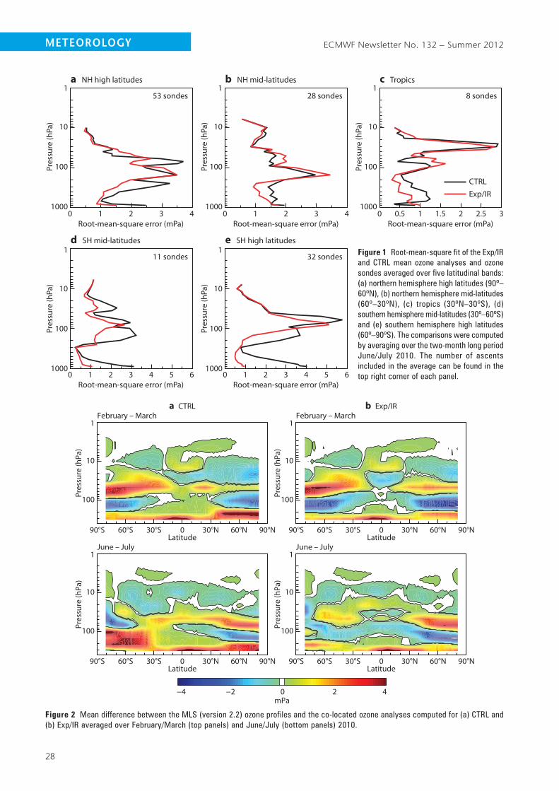
ECMWF Newsletter No. 132 – Summer 2012
28
meteorology
a NH high latitudes b NH mid-latitudes
d SH mid-latitudes e SH high latitudes
c Tropics
53 sondes
CTRLExp/IR
Root-mean-square error (mPa)1.510.50 2 2.5 3
Root-mean-square error (mPa)10 2 3 4
Root-mean-square error (mPa)10 2 3 4
Root-mean-square error (mPa)10 2 3 6
Root-mean-square error (mPa)
Pres
sure
(hPa
)
1
1
10
100
1000
Pres
sure
(hPa
)
1
10
100
1000Pr
essu
re (h
Pa)
1
10
100
1000
Pres
sure
(hPa
)
1
10
100
1000
Pres
sure
(hPa
)
1
10
100
1000
0 2 3 44 55 6
28 sondes
11 sondes 32 sondes
8 sondes
Figure 1 Root-mean-square fit of the Exp/IR and CTRL mean ozone analyses and ozone sondes averaged over five latitudinal bands: (a) northern hemisphere high latitudes (90º–60ºN), (b) northern hemisphere mid-latitudes (60º–30ºN), (c) tropics (30ºN–30ºS), (d) southern hemisphere mid-latitudes (30º–60ºS) and (e) southern hemisphere high latitudes (60º–90ºS). The comparisons were computed by averaging over the two-month long period June/July 2010. The number of ascents included in the average can be found in the top right corner of each panel.
90°S 60°S 30°S 0 30°N 60°N 90°NLatitude
90°S 60°S 30°S 0 30°N 60°N 90°NLatitude
90°S 60°S 30°S 0 30°N 60°N 90°NLatitude
90°S 60°S 30°S 0 30°N 60°N 90°NLatitude
100
10
1
Pres
sure
(hPa
)
February – MarchFebruary – Marchb Exp/IRa CTRL
June – JulyJune – July
100
10
1
Pres
sure
(hPa
)
100
10
1
Pres
sure
(hPa
)
100
10
1
Pres
sure
(hPa
)
−4 −2 0 2 4mPa
Figure 2 Mean difference between the MLS (version 2.2) ozone profiles and the co-located ozone analyses computed for (a) CTRL and (b) Exp/IR averaged over February/March (top panels) and June/July (bottom panels) 2010.
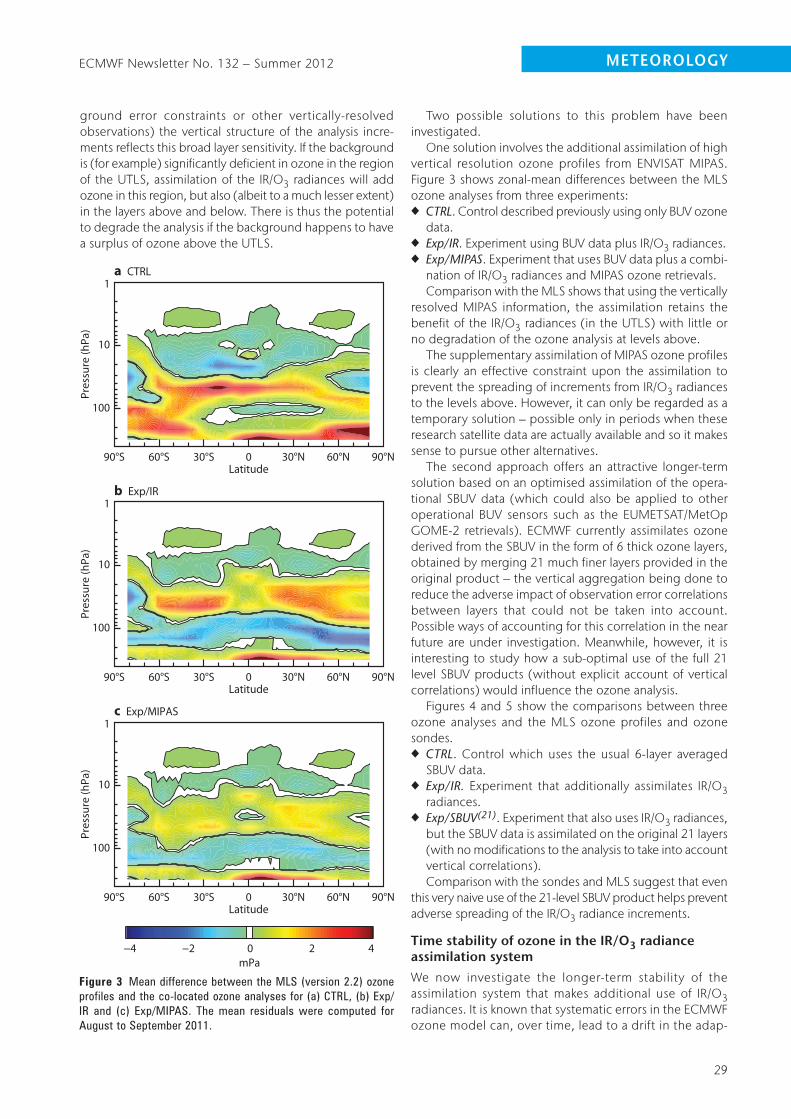
ECMWF Newsletter No. 132 – Summer 2012
29
meteorology
ground error constraints or other vertically-resolved observations) the vertical structure of the analysis incre-ments reflects this broad layer sensitivity. If the background is (for example) significantly deficient in ozone in the region of the UTLS, assimilation of the IR/O3 radiances will add ozone in this region, but also (albeit to a much lesser extent) in the layers above and below. There is thus the potential to degrade the analysis if the background happens to have a surplus of ozone above the UTLS.
Two possible solutions to this problem have been investigated.
One solution involves the additional assimilation of high vertical resolution ozone profiles from ENVISAT MIPAS. Figure 3 shows zonal-mean differences between the MLS ozone analyses from three experiments:u CTRL. Control described previously using only BUV ozone
data.u Exp/IR. Experiment using BUV data plus IR/O3 radiances.u Exp/MIPAS. Experiment that uses BUV data plus a combi-
nation of IR/O3 radiances and MIPAS ozone retrievals.Comparison with the MLS shows that using the vertically
resolved MIPAS information, the assimilation retains the benefit of the IR/O3 radiances (in the UTLS) with little or no degradation of the ozone analysis at levels above.
The supplementary assimilation of MIPAS ozone profiles is clearly an effective constraint upon the assimilation to prevent the spreading of increments from IR/O3 radiances to the levels above. However, it can only be regarded as a temporary solution – possible only in periods when these research satellite data are actually available and so it makes sense to pursue other alternatives.
The second approach offers an attractive longer-term solution based on an optimised assimilation of the opera-tional SBUV data (which could also be applied to other operational BUV sensors such as the EUMETSAT/MetOp GOME-2 retrievals). ECMWF currently assimilates ozone derived from the SBUV in the form of 6 thick ozone layers, obtained by merging 21 much finer layers provided in the original product – the vertical aggregation being done to reduce the adverse impact of observation error correlations between layers that could not be taken into account. Possible ways of accounting for this correlation in the near future are under investigation. Meanwhile, however, it is interesting to study how a sub-optimal use of the full 21 level SBUV products (without explicit account of vertical correlations) would influence the ozone analysis.
Figures 4 and 5 show the comparisons between three ozone analyses and the MLS ozone profiles and ozone sondes.u CTRL. Control which uses the usual 6-layer averaged
SBUV data.u Exp/IR. Experiment that additionally assimilates IR/O3
radiances.u Exp/SBUV(21). Experiment that also uses IR/O3 radiances,
but the SBUV data is assimilated on the original 21 layers (with no modifications to the analysis to take into account vertical correlations).Comparison with the sondes and MLS suggest that even
this very naive use of the 21-level SBUV product helps prevent adverse spreading of the IR/O3 radiance increments.
time stability of ozone in the ir/o3 radiance assimilation system
We now investigate the longer-term stability of the assimilation system that makes additional use of IR/O3 radiances. It is known that systematic errors in the ECMWF ozone model can, over time, lead to a drift in the adap-
100
10
1
Pres
sure
(hPa
)
a CTRL
b Exp/IR
100
10
1
Pres
sure
(hPa
)
c Exp/MIPAS
100
10
1
Pres
sure
(hPa
)
−4 −2 0 2 4mPa
90°S 60°S 30°S 0 30°N 60°N 90°NLatitude
90°S 60°S 30°S 0 30°N 60°N 90°NLatitude
90°S 60°S 30°S 0 30°N 60°N 90°NLatitude
Figure 3 Mean difference between the MLS (version 2.2) ozone profiles and the co-located ozone analyses for (a) CTRL, (b) Exp/IR and (c) Exp/MIPAS. The mean residuals were computed for August to September 2011.
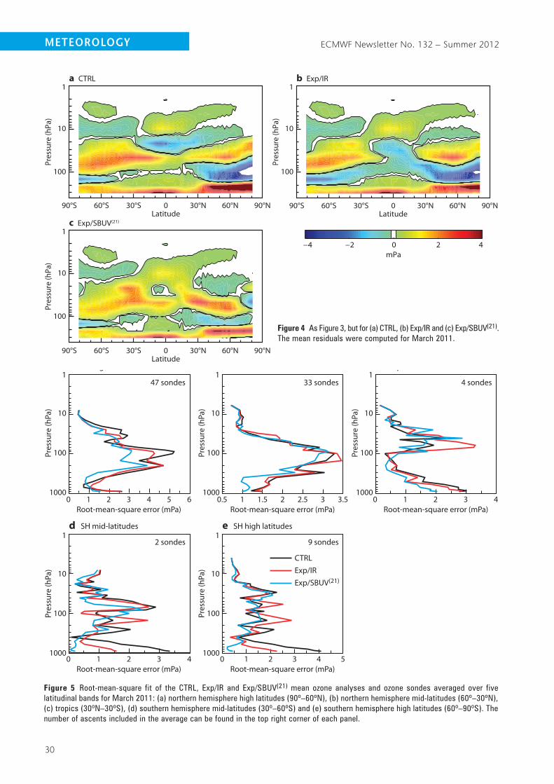
ECMWF Newsletter No. 132 – Summer 2012
30
meteorology
100
10
1
Pres
sure
(hPa
)
a CTRL b Exp/IR
100
10
1
Pres
sure
(hPa
)
c Exp/SBUV(21)
100
10
1
Pres
sure
(hPa
)
−4 −2 0 2 4mPa
90°S 60°S 30°S 0 30°N 60°N 90°NLatitude
90°S 60°S 30°S 0 30°N 60°N 90°NLatitude
90°S 60°S 30°S 0 30°N 60°N 90°NLatitude
a NH high latitudes
47 sondes
CTRLExp/IRExp/SBUV(21)
Root-mean-square error (mPa)Root-mean-square error (mPa)10.5 1.5 2.5 3.52 3
Root-mean-square error (mPa)10 2 3 4 5 6
Root-mean-square error (mPa)10 2 3 5
Root-mean-square error (mPa)
Pres
sure
(hPa
)
1
1
10
100
1000
Pres
sure
(hPa
)
1
10
100
1000
Pres
sure
(hPa
)
1
10
100
1000
Pres
sure
(hPa
)
1
10
100
1000
Pres
sure
(hPa
)
1
10
100
1000
0 2 3 44
10 2 3 4
b NH mid-latitudes
33 sondes
d SH mid-latitudes
2 sondes
e SH high latitudes
9 sondes
c Tropics
4 sondes
Figure 4 As Figure 3, but for (a) CTRL, (b) Exp/IR and (c) Exp/SBUV(21). The mean residuals were computed for March 2011.
Figure 5 Root-mean-square fit of the CTRL, Exp/IR and Exp/SBUV(21) mean ozone analyses and ozone sondes averaged over five latitudinal bands for March 2011: (a) northern hemisphere high latitudes (90º–60ºN), (b) northern hemisphere mid-latitudes (60º–30ºN), (c) tropics (30ºN–30ºS), (d) southern hemisphere mid-latitudes (30º–60ºS) and (e) southern hemisphere high latitudes (60º–90ºS). The number of ascents included in the average can be found in the top right corner of each panel.

ECMWF Newsletter No. 132 – Summer 2012
31
meteorology
tively calculated bias corrections (VarBC) applied to the ozone observations. If unconstrained, this can lead to a corresponding drift in the ozone analysis – which can very quickly develop unrealistic mean ozone states. This drift in bias correction is seen very clearly in a set of previous experiments where only column BUV ozone is assimilated – the data being adaptively bias corrected every analysis cycle against the assimilating model. Figure 6 shows that the corrections drift very quickly and within 30 days can reach values in excess of 20 DU. In the context of this study, the solution adopted was to anchor the analysis mean state against drift by assimilating one observation type (SBUV) with no bias correction and adaptively correcting all other ozone observations to this constrained mean state.
In developing a prototype system to assimilate IR/O3 radiances, Han & McNally addressed the problem of drift by using one channel without correction (channel 1585 from IASI) to anchor the bias correction process. This worked successfully in the short experiments carried out in the aforementioned study – where IR/O3 radiances were the only ozone information assimilated. However, in this context (with a view towards an operational implementation) we must test the longer-term ability of this IASI channel and its corresponding AIRS one (channel 1088) to anchor the ozone analysis – particularly when IR/O3 radiances are used in combination with BUV ozone observations. These alterna-tives for anchoring the ozone analysis against drift have been tested in a pair of parallel assimilations that have been run over a full calendar year:u CTRL. Control that uses all available BUV data (SBUV, OMI
and SCIAMACHY) – anchored by the SBUV data being assimilated without bias correction.
u Exp/IR. Experiment that additionally assimilates IR/O3 radiances, but applies VarBC adaptive bias corrections to all BUV data (including SBUV) and uses two uncor-rected IR/O3 channels to anchor the system.To display the time evolution of ozone in these experi-
ments in a concise way, ozone changes are now integrated in the vertical and presented in terms of total column values. Figure 7 shows a time series of the difference between the zonally-averaged total column ozone from the Exp/IR and
CTRL analyses. It is clear that the assimilation of the IR/O3 channels initially increases the analyzed column ozone at all latitudes (typically just 1–2 DU in the first month), but this increase continues to grow steadily in time, such that in less than a year the column differences have reached values as large as 30 DU.
To assess the realism of these significant changes to the mean column ozone, we again compare the analyses to the MLS. Integrated columns from the experiment and control analyses are computed over vertical domain of the MLS between 0.1 and 215 hPa and collocated to the MLS locations. In Figure 8 yellow to red colours show areas where the MLS has higher column ozone values than the analyses; the green to purple colours are where MLS has lower values. Initially the increase in ozone concentration at lower levels from the assimilation of IR/O3 radiances (reported in previous sections) provides a marked improve-ment in the fit of total column ozone to MLS in the southern hemisphere and tropics compared to the control. But it is
Bias
cor
rect
ion
(DU
)
30Number of days
40 502010
-20
-15
-10
-5
0
SCIAMACHYOMI
NOAA-18 SBUV/2NOAA-17 SBUV/2
2 Jan2010
1 Feb 3 Mar 2 Apr 2 May 1 Jun 1 Jul 5 Aug 4 Sep 4 Oct 3 Nov
Exp/IR – CTRL DU
03691215182124273090°N
60°N
30°N
0°
30°S
60°S
90°S
Latit
ude
Figure 6 Evolution of the global bias correction applied to four ozone products assimilated in a low-resolution version of the ECMWF system that did not use IR/O3. The thin and thick black lines refer to OMI and SCIAMACHy total column ozone, respectively. The thin and the thick green lines refer to the bottom layer (1013–16 hPa) of NOAA-17 and NOAA-18 SBUV/2, respectively.
Figure 7 Hovmöller plot of the total column ozone residuals between the CTRL and Exp/IR experiments. Units are DU.

ECMWF Newsletter No. 132 – Summer 2012
32
meteorology
1 Jan 5 Feb 5 Mar 2 Apr 7 May 4 Jun 3 Jul 7 Aug 4 Sep 2 Oct 6 Nov
MLS – CTRL DU35
25
15
5
–5
–15
–25
–35
90°N
60°N
30°N
0
30°S
60°S
90°S
Latit
ude
90°N
60°N
30°N
0
30°S
60°S
90°S
Latit
ude
1 Jan 5 Feb 5 Mar 2 Apr 7 May 4 Jun 3 Jul 7 Aug 4 Sep 2 Oct 6 Nov
MLS – Exp/IR
2010
2010
Figure 8 Hovmöller plots of the integrated column ozone difference between the MLS version 2.2 ozone profiles and co-located ozone analyses from CTRL (top) and Exp/IR (bottom), computed between 0.1 and 215 hPa. The black contour line shows the zero difference line. Data are in DU.
clear that the column ozone continues to increase and is far in excess of the control and the values measured by the MLS suggesting that the IR/O3 system has drifted to an unrealistic state. An examination of the adaptive bias corrections computed for the BUV instruments within the IR/O3 system shows the characteristic inflation to very large negative values. Consequently, we must conclude that the use of just two IR/O3 channels is insufficient to anchor the ozone column as a whole against longer-term drifting due to model error.
The obvious solution is to reinstate the assimilation of uncorrected SBUV as an additional anchor when the IR/O3 radiances are assimilated. While it was impractical to re-run the full one-year experiment, short additional periods (capturing the periods when the drift was most pronounced) have been tested and confirm the effectiveness of the combined IR and SBUV anchor.
An experiment run between May 2011 and September 2011 is shown in Figure 9. Up until the 12 July this used only the two IR/O3 channels as an anchor and the charac-teristic drift in the ozone analysis relative to the CTRL can clearly be seen (Figure 9a). However, after this date the SBUV anchor was reinstated in addition to the IR/O3 chan-nels, causing the drift to stop and revert backwards to lower
ozone values. Following the change, comparison with the MLS column data (Figures 9b and 9c) shows the ozone analysis to be stable and in significantly better agreement with the MLS than the control ozone analysis.
overview
This study has shown that IR/O3 radiances from AIRS, IASI and HIRS can be successfully used to complement the exist-ing BUV ozone data – providing additional information in the absence of sunlight and in the UTLS. The combined IR plus BUV ozone analyses agree significantly better with independent ozone information from sondes and the Aura MLS compared to an ozone analysis based on BUV data alone. As expected the main benefits are seen at altitudes below the ozone maximum in the region of the UTLS – particularly at high latitudes in the wintertime (when sunlight is limited).
Some vertical spreading of the analysis increments due to the IR/O3 radiances can occasionally cause a slight degradation of ozone above the UTLS. This is not consid-ered a severe problem and can be tolerated in view of the greater benefits brought by the radiance data. However, it has been shown that this spreading can be effectively constrained by providing the analysis with vertically-

ECMWF Newsletter No. 132 – Summer 2012
33
meteorology
resolved ozone information above the UTLS from either MIPAS profiles – or indeed the operationally available SBUV used on its original 21 layers.
Longer-running experiments (in this and previous studies) have shown that the ozone analysis needs to be anchored to avoid model drift adversely affecting the VarBC bias corrections. Results clearly indicate that the use of just two IR/O3 anchor channels is insufficient to stabilize the analysis in the longer term and these must
Exp/IR – CTRL TCO
-12-9-6-303691215182190°N
60°N
30°N
0°
30°S
60°S
90°S
90°N
60°N
30°N
0°
30°S
60°S
90°S
90°N
60°N
30°N
0°
30°S
60°S
90°S
DU
DU
35
25
15
5
–5
–15
–25
–35
12 May2011
1 Jun
12 May
12 May
1 Jun
1 Jul 2 Aug 1 Sep
2011
No MLS data available
No MLS data available
2011
1 Jul 2 Aug 1 Sep
MLS – CTRL
Latit
ude
Latit
ude
Latit
ude
MLS – Exp/IR
1 Jun 1 Jul 2 Aug 1 Sep
Figure 9 As for Figure 7 (top panel) and Figure 8 (middle and bottom panels), but when the ozone bias correction of the Exp/IR experiment was anchored to two IR/O3 channels until 12 July, and to the additional SBUV ozone data afterwards. Note that MLS data was unavailable during the first part of the period.
be supplemented by anchoring information from the assimilation of uncorrected SBUV.
FUrtHer readingHan, w. & a.P. mcnally, 2010. The 4D-Var assimilation of ozone-sensitive infrared radiances measured by IASI. Q. J. R. Meteorol. Soc, 136, 2025–2037.Jackson, d. & r. saunders, 2002. Ozone data assimilation: preliminary system. Technical Report 394, Met Office.

34
BUFR data and MetviewVESA KARHILA, SáNDOR KERTéSz, IAIN RUSSELL, STEPHAN SIEMEN
BUFR has a reputation of being complex and difficult to use. With this article we want to show how Metview can be used to handle BUFR data easily and efficiently.
BUFR, like GRIB, is binary: it requires software to decode it. ECMWF provides a software package BUFRDC to handle BUFR data, but this package requires some expertise to use. Metview has an internal higher-level wrapper around the basic BUFRDC library, making it much easier for Metview developers to write tools to handle BUFR data. As a result, Metview has always provided practical solutions for handling BUFR data and the development of such tools continues in Metview 4. For instance, since version 4.3.0 Metview has been able to decode also PrepBUFR files. With Metview we can easily examine, extract, plot, overlay and process BUFR data. An overview of BUFR is given in Box A.
BUFR data stored in MARS can be accessed with a Metview Mars Retrieval icon. Files containing BUFR messages are automatically shown with a BUFR icon (Figure 1a) in the Metview Desktop.
Plotting BUFr data
Metview can plot some types of BUFR data directly (mainly some traditional WMO observation types for which WMO has defined a plotting scheme) simply by right-clicking the icon and selecting Visualise from the pop-up menu. To customise which values to include (or exclude) from a plot, we use the Observation Plotting icon (Figure 1b). An example plot of TEMP data is shown in Figure 2.
To plot any other types of BUFR data we need to extract the required data values and locations into geopoints or CSV (Comma Separated Values) format (see below) and then plot these values. BUFR data can be overlaid with any other data types in a Metview plot.
examining BUFr data
In order to extract values from BUFR data we need to know what data is stored in a BUFR file. Bufr Examiner is Metview’s tool to study the contents of BUFR files. It is available from
a
d
b
e
c
f
Figure 1 Icons representing (a) BUFR data, (b) Observation Plotting visual definition, (c) Observation Filter tool, (d) BufrPicker tool, (e) OperaRadarFilter tool and (f) Geopoints to Grib tool.
BUFr and PrepBUFr
BUFR
BUFR (Binary Universal Form for Representation of mete-orological data) is a WMO standard for transmitting and storing observed meteorological data. BUFR is flexible – it can be used to store very different data, ranging from traditional SYNOP and TEMP observations to modern satellite and radar observations.
Data stored in BUFR messages are identified by data descriptors. Data descriptors are keys to the BUFR data. To access any data values from BUFR messages, we need to know the data descriptor of the data type.
BUFR is a ‘Table Driven Code Form’. This code form is based on the idea that part of the metadata, including the values used for coding, is stored in external table files. This is one strong point of BUFR (messages are smaller), but it becomes a weak point if something is wrong with the required external table files.
PrepBUFRBUFR is so flexible that it is possible to encode BUFR tables in BUFR format. NCEP (National Centers for Environmental Prediction, USA) creates BUFR files, called PrepBUFR, where BUFR messages containing meteorological data are preceded by messages that contain the BUFR table entries required to decode the data part. This method avoids all table related errors in decoding, but it sets new require-ments for the decoding software.
a
Figure 2 An example plot of TEMP (upper-air sounding) data.
ECMWF Newsletter No. 132 – Summer 2012ComPUting

ECMWF Newsletter No. 132 – Summer 2012
35
ComPUting
the context menu of a BUFR icon. Bufr Examiner was com pletely re-written for Metview 4 and the new version provides options to search and to customise the output. An example output of Bufr Examiner is shown in Figure 3.
extracting data values from BUFr files
Metview provides several modules to extract values from BUFR files, for plotting or for further processing. Data descriptors (as shown in the Descriptor column in the Bufr Examiner data tab output) are used to define which data should be extracted.
Observation Filter, or ObsFilter for short, can be used to filter BUFR data in two ways. First, ObsFilter can be used to select a subset of BUFR messages from a BUFR file, accord-ing to time, type, location, etc. The result is still in BUFR format. Second, ObsFilter can be used to extract scalar (or vector) values from BUFR messages (from all messages or from a subset) into geopoints, geovectors or CSV format. Geopoints and geovectors are custom Metview ASCII formats for scattered geospatial data. ObsFilter icon is shown in Figure 1c and an example plot in Figure 4.
Figure 3 Metview’s Bufr Examiner, showing a list of messages (left), the data from the selected message (right), information about the file (top) and a log area which reports any errors encountered when decoding the file (bottom).
Figure 4 An example plot of temperature values extracted from BUFR data using ObsFilter. The histogram legend shows the distribution of the data.
Figure 5 Brightness temperature values from the AMSU-A sensor onboard MetOp-A visualised in Metview 4. The values were extracted from the original BUFR file by Metview’s BufrPicker.
Figure 6 OPERA BUFR image overlaid with the corresponding mean-sea-level pressure analysis from ECMWF’s MARS archive.
Figure 7 An example plot of departures of a 2-metre temperature field from observed values.
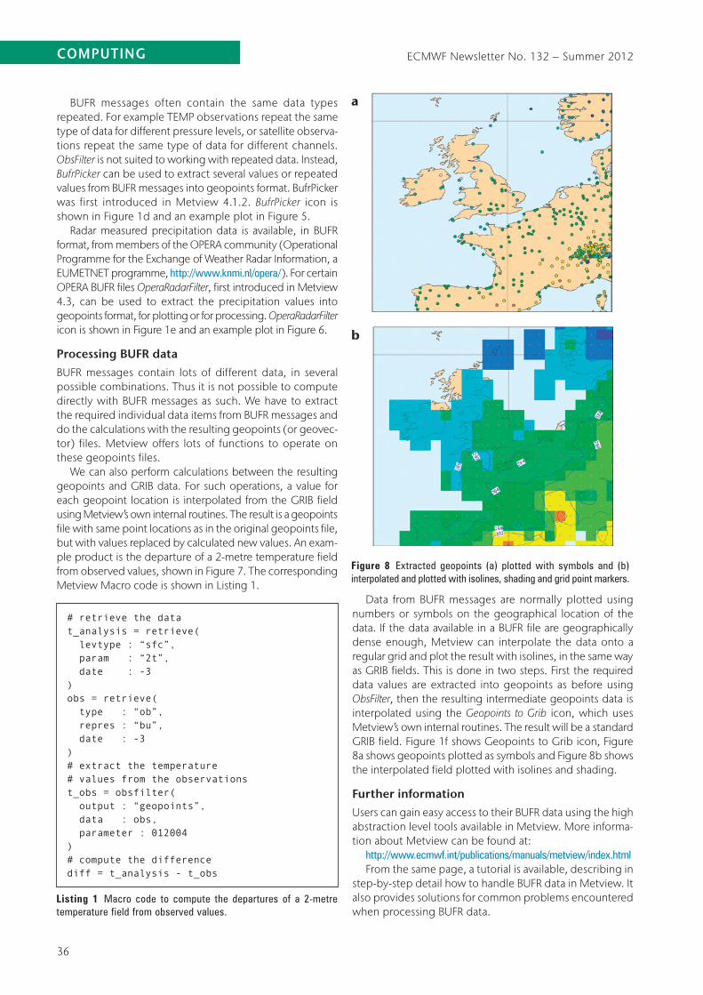
BUFR messages often contain the same data types repeated. For example TEMP observations repeat the same type of data for different pressure levels, or satellite observa-tions repeat the same type of data for different channels. ObsFilter is not suited to working with repeated data. Instead, BufrPicker can be used to extract several values or repeated values from BUFR messages into geopoints format. BufrPicker was first introduced in Metview 4.1.2. BufrPicker icon is shown in Figure 1d and an example plot in Figure 5.
Radar measured precipitation data is available, in BUFR format, from members of the OPERA community (Operational Programme for the Exchange of Weather Radar Information, a EUMETNET programme, http://www.knmi.nl/opera/). For certain OPERA BUFR files Opera Radar Filter, first introduced in Met view 4.3, can be used to extract the precipitation values into geopoints format, for plotting or for processing. Opera Radar Filter icon is shown in Figure 1e and an example plot in Figure 6.
Processing BUFr data
BUFR messages contain lots of different data, in several possible combi na tions. Thus it is not possible to compute directly with BUFR messages as such. We have to extract the required individual data items from BUFR messages and do the calculations with the resulting geopoints (or geovec-tor) files. Metview offers lots of functions to operate on these geopoints files.
We can also perform calculations between the resulting geopoints and GRIB data. For such operations, a value for each geopoint location is interpolated from the GRIB field using Metview’s own internal routines. The result is a geopoints file with same point locations as in the original geopoints file, but with values replaced by calculated new values. An exam-ple product is the departure of a 2-metre temperature field from observed values, shown in Figure 7. The corresponding Metview Macro code is shown in Listing 1.
Data from BUFR messages are normally plotted using numbers or symbols on the geographical location of the data. If the data available in a BUFR file are geographically dense enough, Metview can interpolate the data onto a regular grid and plot the result with isolines, in the same way as GRIB fields. This is done in two steps. First the required data values are extracted into geopoints as before using ObsFilter, then the resulting intermediate geopoints data is interpolated using the Geopoints to Grib icon, which uses Metview’s own internal routines. The result will be a standard GRIB field. Figure 1f shows Geopoints to Grib icon, Figure 8a shows geopoints plotted as symbols and Figure 8b shows the interpolated field plotted with isolines and shading.
Further information
Users can gain easy access to their BUFR data using the high abstraction level tools available in Metview. More informa-tion about Metview can be found at:
http://www.ecmwf.int/publications/manuals/metview/index.htmlFrom the same page, a tutorial is available, describing in
step-by-step detail how to handle BUFR data in Metview. It also provides solutions for common problems encountered when processing BUFR data.
# retrieve the datat_analysis = retrieve( levtype : “sfc”, param : “2t”, date : -3)obs = retrieve( type : “ob”, repres : “bu”, date : -3)# extract the temperature# values from the observationst_obs = obsfilter( output : “geopoints”, data : obs, parameter : 012004)# compute the differencediff = t_analysis - t_obs
Listing 1 Macro code to compute the departures of a 2-metre temperature field from observed values.
Figure 8 Extracted geopoints (a) plotted with symbols and (b) interpolated and plotted with isolines, shading and grid point markers.
a
b
ECMWF Newsletter No. 132 – Summer 2012
36
ComPUting

ECMWF Newsletter No. 132 – Summer 2012
37
ECMWF Calendar 2012
October 1 – 5 15th Workshop on ‘High performance computing in meteorology’
October 8 – 12 Training Course – Use and interpretation of ECMWF products for WMO Members
October 15 – 17 Scientific Advisory Committee (41st Session)
October 18 – 19 Technical Advisory Committee (44th Session)
October 22–24 Workshop on ‘Atmospheric Composition Observation System Simulation Experiments (OSSE)
October 22 – 23 Finance Committee (91st Session)
October 24 – 25 Policy Advisory Committee (34th Session)
November 1 Advisory Committee of Co-operating States (18th Session, Geneva)
November 5 – 8 Workshop on ‘Parametrization of clouds and precipitation across model resolution’
December 4 – 5 Council (78th Session)
general
ECMWF publications(see http://www.ecmwf.int/publications/)
technical memoranda683 Manrique Suñén, A., A. Nordbo, G. Balsamo, A. Beljaars
& I. Mammarella: Representing land surface hetero-geneity with the tiling method: merits and limitations in presence of large contrast. July 2012
682 Hirons, L.C., P. Inness, F. Vitart & P. Bechtold: Under-standing advances in the simulation of intraseasonal variability in the ECMWF model. Part II: The applica-tion of process-based diagnostics. June 2012
681 Hirons, L.C., P. Inness, F. Vitart & P. Bechtold: Under-standing advances in the simulation of intraseasonal variability in the ECMWF model. Part I: The represen-tation of the MJO. July 2012
679 Radnoti, G., P. Bauer, A. McNally & A. Horanyi: ECMWF study to quantify the interaction between terrestrial and space-based observing systems on Numerical Weather Prediction skill. May 2012
676 Magnusson, L., M. Alonso-Balmaseda, S. Corti, F. Molteni & T. Stockdale: Evaluation of forecast strategies for seasonal and decadal forecasts in presence of system-atic model errors. June 2012
675 Boussetta, S., G. Balsamo, A. Beljaars, A. Agusti-Panareda, J.-C. Calvet, C. Jacobs, B. van den Hurk, P. Viterbo, S. Lafont, E. Dutra, L. Jarlan, M. Balzarolo, D. Papale & G. van der Werf: Natural carbon dioxide exchanges in the ECMWF Integrated Forecasting System: Implementation and offline validation. May 2012
671 Inness, A., F. Baier, A. Benedetti, I. Bouarar, S. Chabrillat, H. Clark, C. Clerbaux, P. Coheur, R.J. Engelen, Q. Errera, J. Flemming, M. George, C. Granier, J. Hadji-Lazaro, V. Huijnen, D. Hurtmans, L. Jones, J.W. Kaiser, J. Kapsomenakis, K. Lefever, J. Leitão, M. Razinger, A. Richter, M.G. Schultz, A.J. Simmons, M. Suttie, O. Stein, V. Thouret, M. Vrekoussis, C. Zerefos & the MACC Team: The MACC reanalysis: An 8-year data set of atmospheric composition. May 2012
Index of newsletter articlesThis is a selection of articles published in the ECMWF Newsletter series during recent years.
Articles are arranged in date order within each subject category. Articles can be accessed on the ECMWF public website – www.ecmwf.int/publications/newsletter/index.html
No. Date Page
newsNCEP joins EUROSIP 132 Summer 2012 4
Forecast Products Users’ Meeting, June 2012 132 Summer 2012 4
ECMWF Annual Report for 2011 132 Summer 2012 5
Ocean wave forecasting 132 Summer 2012 6
No. Date PageMember and Co-operating State visits: new cycle 2011–2013 132 Summer 2012 7Optimising the number of GNSS radio occultation measurements 132 Summer 2012 8NWP training courses 2012: Interesting, informative and relevant 132 Summer 2012 9

ECMWF Newsletter No. 132 – Summer 2012
38
general
No. Date Page
newsOptical turbulence modelling for astronomical applications 132 Summer 2012 9Plots of the long-term evolution of operational forecast skill updated 132 Summer 2012 11Development of a new ECMWF website 131 Spring 2012 2Migration of the MARS system to a Linux cluster 131 Spring 2012 4Training courses: a success story 131 Spring 2012 5Bias correction of aircraft data implemented in November 2011 131 Spring 2012 6RMDCN – Next Generation 131 Spring 2012 7Introduction to the science of weather and weather forecasting 131 Spring 2012 8ECMWF’s plans for 2012 130 Winter 2011/12 2Honorary degree awarded to Alan Thorpe 130 Winter 2011/12 2 2Co-operation with EFAS 130 Winter 2011/12 3Diurnal cycles and the stable atmospheric boundary layer 130 Winter 2011/12 5Accession agreement between Croatia and ECMWF 130 Winter 2011/12 6Applying for computing resources for Special Projects 130 Winter 2011/12 7Outcome of Council’s 76th session 130 Winter 2011/12 7Establishment of Atmospheric Composition Division 130 Winter 2011/12 8Revision of the surface roughness length table 130 Winter 2011/12 8Use and development of Meteorological Operational Systems 130 Winter 2011/12 10Upgrade of the HPCF 130 Winter 2011/12 11Progress in ERA-CLIM: First General Assembly 130 Winter 2011/12 12New model cycle 37r3 130 Winter 2011/12 13Departure of Ute Dahremöller 129 Autumn 2011 2Flow-dependent background error variance in 4D-Var 129 Autumn 2011 2Election of Dominique Marbouty as EMS President 129 Autumn 2011 3ECMWF workshops and scientific meetings in 2012 129 Autumn 2011 4Better Internet access to ERA-Interim 129 Autumn 2011 6An appreciation of Dominique Marbouty 128 Summer 2011 2Outcome of Council’s 75th session 128 Summer 2011 3Jean Labrouse 128 Summer 2011 4Forecast Products Users’ Meeting, June 2011 128 Summer 2011 5IMO Prize for the first ECMWF Director 128 Summer 2011 6Extension of the ERA-Interim reanalysis to 1979 128 Summer 2011 7Representing model uncertainty and error in weather and climate prediction 128 Summer 2011 9New model cycle 37r2 128 Summer 2011 10Internal reorganisation within the Research and Operations Departments 127 Spring 2011 3New Member States 127 Spring 2011 5New Director-General of ECMWF from July 2011 126 Winter 2010/11 274th Council session on 7–8 December 2010 126 Winter 2010/11 4Non-hydrostatic modelling 126 Winter 2010/11 6
No. Date Page
newsNew interactive web tool for forecasters 126 Winter 2010/11 7Symposium to honour Martin Miller 126 Winter 2010/11 9
CoMputingBUFR data and Metview 132 Summer 2012 34A new trajectory interface in Metview 4 131 Spring 2012 31A new framework to handle ODB in Metview 4 130 Winter 2011/12 31Managing work flows with ecFlow 129 Autumn 2011 30Support for OGC standards in Metview 4 127 Spring 2011 28Metview 4 – ECMWF’s latest generation meteorological workstation 126 Winter 2010/11 23Green computing 126 Winter 2010/11 28Metview Macro – A powerful meteorological batch language 125 Autumn 2010 30The Data Handling System 124 Summer 2010 31Update on the RMDCN 123 Spring 2010 29Magics++ 2.8 – New developments in ECMWF’s meteorological graphics library 122 Winter 2009/10 32The EU-funded BRIDGE project 117 Autumn 2008 29ECMWF’s Replacement High Performance Computing Facility 2009–2013 115 Spring 2008 44
Meteorology
Observations & AssimilationTowards an operational GMES Atmosphere Monitoring Service 132 Summer 2012 20Blending information from infrared radiances with ultraviolet data in the operational ozone analysis 132 Summer 2012 26Use of EDA-based background error variances in 4D-Var 130 Winter 2011/12 24Observation errors and their correlations for satellite radiances 128 Summer 2011 17Development of cloud condensate background errors 128 Summer 2011 23Use of SMOS data at ECMWF 127 Spring 2011 23Extended Kalman Filter soil-moisture analysis in the IFS 127 Spring 2011 12Weak constraint 4D-Var 125 Autumn 2010 12Surface pressure information derived from GPS radio occultation measurements 124 Summer 2010 24Quantifying the benefit of the advanced infrared sounders AIRS and IASI 124 Summer 2010 29Collaboration on Observing System Simulation Experiments (Joint OSSE) 123 Spring 2010 14The new Ensemble of Data Assimilations 123 Spring 2010 17Assessment of FY-3A satellite data 122 Winter 2009/10 18Huber norm quality control in the IFS 122 Winter 2009/10 27The direct assimilation of cloud-affected infrared radiances in the ECMWF 4D-Var 120 Summer 2009 32The new all-sky assimilation system for passive microwave satellite imager observations 121 Autumn 2009 7
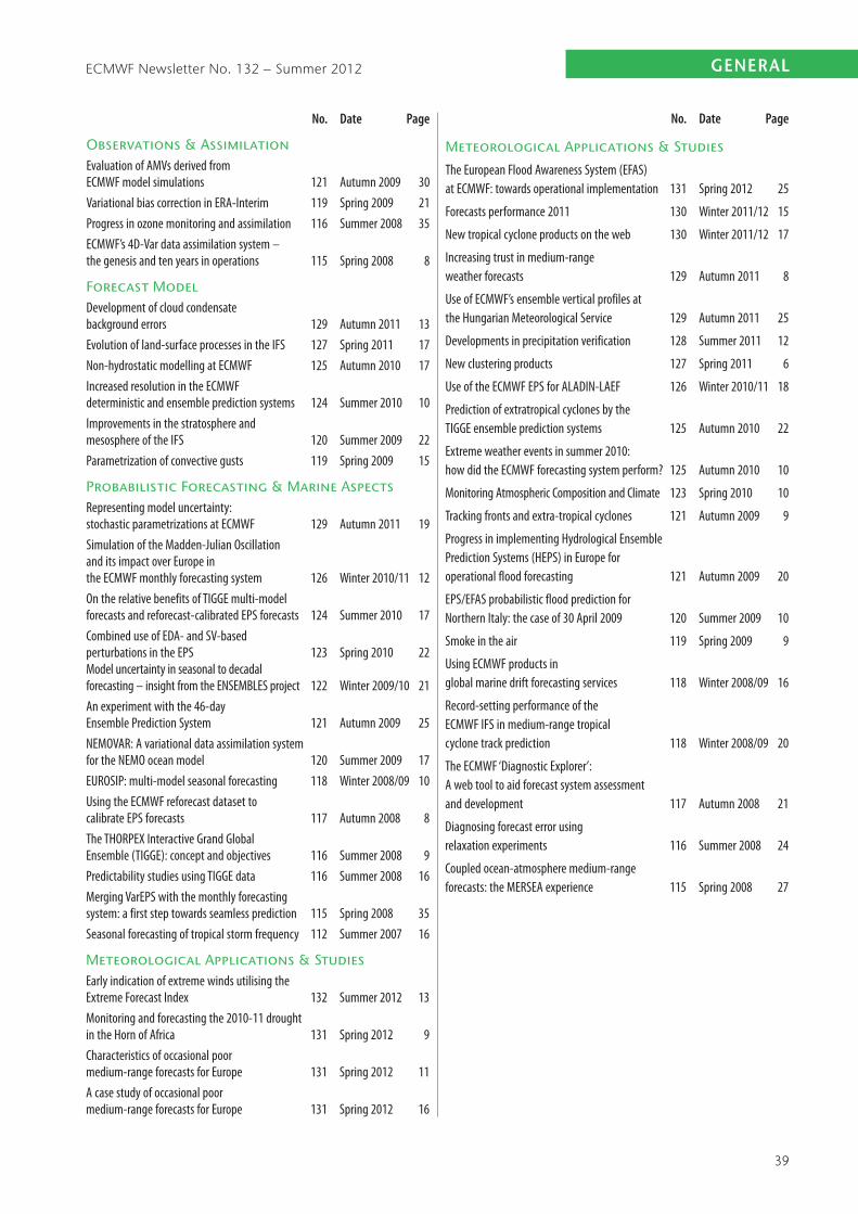
ECMWF Newsletter No. 132 – Summer 2012
39
general
No. Date Page
Observations & AssimilationEvaluation of AMVs derived from ECMWF model simulations 121 Autumn 2009 30Variational bias correction in ERA-Interim 119 Spring 2009 21Progress in ozone monitoring and assimilation 116 Summer 2008 35ECMWF’s 4D-Var data assimilation system – the genesis and ten years in operations 115 Spring 2008 8
Forecast ModelDevelopment of cloud condensate background errors 129 Autumn 2011 13Evolution of land-surface processes in the IFS 127 Spring 2011 17Non-hydrostatic modelling at ECMWF 125 Autumn 2010 17Increased resolution in the ECMWF deterministic and ensemble prediction systems 124 Summer 2010 10Improvements in the stratosphere and mesosphere of the IFS 120 Summer 2009 22Parametrization of convective gusts 119 Spring 2009 15
Probabilistic Forecasting & Marine AspectsRepresenting model uncertainty: stochastic parametrizations at ECMWF 129 Autumn 2011 19Simulation of the Madden-Julian Oscillation and its impact over Europe in the ECMWF monthly forecasting system 126 Winter 2010/11 12On the relative benefits of TIGGE multi-model forecasts and reforecast-calibrated EPS forecasts 124 Summer 2010 17Combined use of EDA- and SV-based perturbations in the EPS 123 Spring 2010 22 Model uncertainty in seasonal to decadal forecasting – insight from the ENSEMBLES project 122 Winter 2009/10 21An experiment with the 46-day Ensemble Prediction System 121 Autumn 2009 25NEMOVAR: A variational data assimilation system for the NEMO ocean model 120 Summer 2009 17EUROSIP: multi-model seasonal forecasting 118 Winter 2008/09 10Using the ECMWF reforecast dataset to calibrate EPS forecasts 117 Autumn 2008 8The THORPEX Interactive Grand Global Ensemble (TIGGE): concept and objectives 116 Summer 2008 9Predictability studies using TIGGE data 116 Summer 2008 16Merging VarEPS with the monthly forecasting system: a first step towards seamless prediction 115 Spring 2008 35Seasonal forecasting of tropical storm frequency 112 Summer 2007 16
Meteorological Applications & StudiesEarly indication of extreme winds utilising the Extreme Forecast Index 132 Summer 2012 13Monitoring and forecasting the 2010-11 drought in the Horn of Africa 131 Spring 2012 9Characteristics of occasional poor medium-range forecasts for Europe 131 Spring 2012 11A case study of occasional poor medium-range forecasts for Europe 131 Spring 2012 16
No. Date Page
Meteorological Applications & Studies
The European Flood Awareness System (EFAS) at ECMWF: towards operational implementation 131 Spring 2012 25
Forecasts performance 2011 130 Winter 2011/12 15
New tropical cyclone products on the web 130 Winter 2011/12 17
Increasing trust in medium-range weather forecasts 129 Autumn 2011 8
Use of ECMWF’s ensemble vertical profiles at the Hungarian Meteorological Service 129 Autumn 2011 25
Developments in precipitation verification 128 Summer 2011 12
New clustering products 127 Spring 2011 6
Use of the ECMWF EPS for ALADIN-LAEF 126 Winter 2010/11 18
Prediction of extratropical cyclones by the TIGGE ensemble prediction systems 125 Autumn 2010 22
Extreme weather events in summer 2010: how did the ECMWF forecasting system perform? 125 Autumn 2010 10
Monitoring Atmospheric Composition and Climate 123 Spring 2010 10
Tracking fronts and extra-tropical cyclones 121 Autumn 2009 9
Progress in implementing Hydrological Ensemble Prediction Systems (HEPS) in Europe for operational flood forecasting 121 Autumn 2009 20
EPS/EFAS probabilistic flood prediction for Northern Italy: the case of 30 April 2009 120 Summer 2009 10
Smoke in the air 119 Spring 2009 9
Using ECMWF products in global marine drift forecasting services 118 Winter 2008/09 16
Record-setting performance of the ECMWF IFS in medium-range tropical cyclone track prediction 118 Winter 2008/09 20
The ECMWF ‘Diagnostic Explorer’: A web tool to aid forecast system assessment and development 117 Autumn 2008 21
Diagnosing forecast error using relaxation experiments 116 Summer 2008 24
Coupled ocean-atmosphere medium-range forecasts: the MERSEA experience 115 Spring 2008 27

ECMWF Newsletter No. 132 – Summer 2012
40
general
ext
Director-GeneralAlan Thorpe 001
Deputy Director-General & Director of OperationsWalter Zwieflhofer 003
Director of ResearchErland Källén 005
Director of Administration DepartmentNyall Farrell 007
SwitchboardECMWF switchboard 000
AdvisoryInternet mail addressed to [email protected] Telefax (+44 118 986 9450, marked User Support)
Computer DivisionDivision Head Isabella Weger 050Computer Operations Section Head Matthias Nethe 363Networking and Computer Security Section Head Rémy Giraud 356Servers and Desktops Section Head Duncan Potter 355Systems Software Section Head Michael Hawkins 353User Support Section Head Umberto Modigliani 382User Support Staff Paul Dando 381 Dominique Lucas 386 Carsten Maaß 389 Pam Prior 384 Christian Weihrauch 380
Computer OperationsCall Desk 303 Call Desk email: [email protected] – Shift Leaders 803 Console fax number +44 118 949 9840 Console email: [email protected] reporting – Call Desk 303Registration – Call Desk 303Service queries – Call Desk 303Tape Requests – Tape Librarian 315
extMeteorological DivisionDivision Head Erik Andersson 060Data Services Group Leader Fabio Venuti 422Meteorological Applications Section Head Alfred Hofstadler 400Meteorological Data Section Head Baudouin Raoult 404Meteorological Visualisation Section Head Stephan Siemen 375 Meteorological Operations Section Head David Richardson 420Meteorological Analysts Antonio Garcia-Mendez 424 Anna Ghelli 425 Martin Janousek 460 Fernando Prates 421 Meteorological Operations Room 426Data DivisionDivision Head Jean-Noël Thépaut 030Data Assimilation Section Head Lars Isaksen 852Satellite Data Section Head Stephen English 660Reanalysis Section Head Dick Dee 352Predictability DivisionDivision Head Roberto Buizza 653Marine Aspects Section Head Peter Janssen 116Probabilistic Forecasting Section Head Franco Molteni 108Model DivisionDivision Head Peter Bauer 080Numerical Aspects Section Head Agathe Untch 704Physical Aspects Section Head Anton Beljaars 035Atmospheric Composition DivisionDivision Head Vincent-Henri Peuch 102Chemical Aspects Section Head Richard Engelen 606
Education & TrainingSarah Keeley 436
ECMWF library & documentation distributionEls Kooij-Connally 751
Useful names and telephone numbers within ECMWFTelephone
Telephone number of an individual at the Centre is:International: +44 118 949 9 + three digit extension UK: (0118) 949 9 + three digit extension Internal: 2 + three digit extensione.g. the Director-General’s number: +44 118 949 9001 (international), (0118) 949 9001 (UK) and 2001 (internal).
The e-mail address of an individual at the Centre is: [email protected]. the Director-General’s address: [email protected]
For double-barrelled names use a hyphen e.g. [email protected]
ECMWF’s public web site: www.ecmwf.int