continuous analogues of matrix factorizations
TRANSCRIPT
Continuous analogues of matrixfactorizationsNASC seminar, 9th May 2014
Alex TownsendDPhil student
Mathematical InstituteUniversity of Oxford
(joint work with Nick Trefethen)
Many thanks to Gil Strang, MIT. Work supported by supported by EPSRC grant EP/P505666/1.

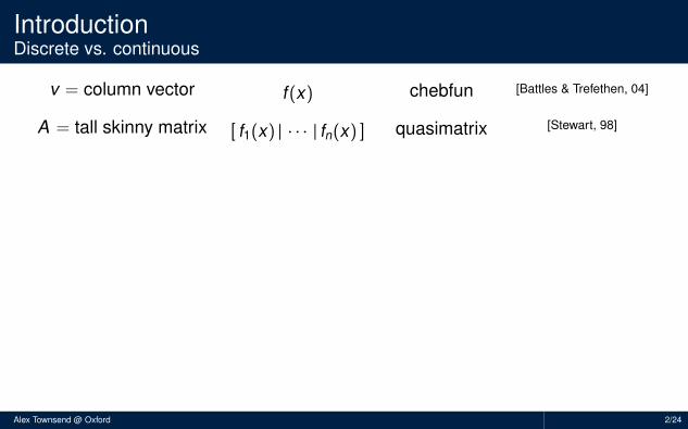
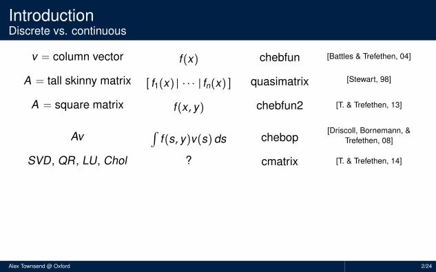
IntroductionDiscrete vs. continuous
v = column vector
A = tall skinny matrix
A = square matrix
Av
SVD, QR, LU, Chol
f(x)
[ f1(x) | · · · | fn(x) ]
f(x , y)∫f(s, y)v(s) ds
?
chebfun
quasimatrix
chebfun2
chebop
cmatrix
[Battles & Trefethen, 04]
[Stewart, 98]
[T. & Trefethen, 13]
[Driscoll, Bornemann, &Trefethen, 08]
[T. & Trefethen, 14]
Interested in continuous analogues rather than infinite analogues.
Aside: Infinite analogues are Schmidt, Wiener–Hopf, infinite-dimensional QR, etc.
Alex Townsend @ Oxford 2/24
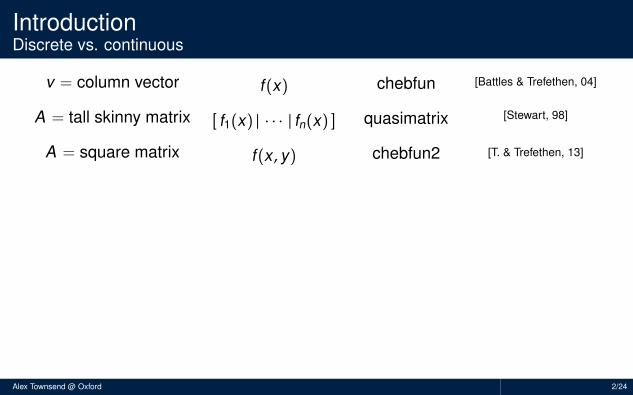
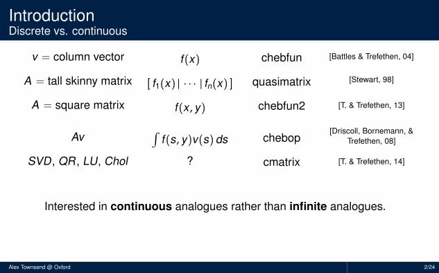
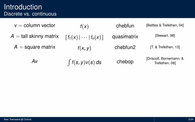
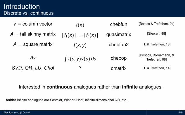
IntroductionDiscrete vs. continuous
v = column vector
A = tall skinny matrix
A = square matrix
Av
SVD, QR, LU, Chol
f(x)
[ f1(x) | · · · | fn(x) ]
f(x , y)
∫f(s, y)v(s) ds
?
chebfun
quasimatrix
chebfun2
chebop
cmatrix
[Battles & Trefethen, 04]
[Stewart, 98]
[T. & Trefethen, 13]
[Driscoll, Bornemann, &Trefethen, 08]
[T. & Trefethen, 14]
Interested in continuous analogues rather than infinite analogues.
Aside: Infinite analogues are Schmidt, Wiener–Hopf, infinite-dimensional QR, etc.
Alex Townsend @ Oxford 2/24
IntroductionDiscrete vs. continuous
v = column vector
A = tall skinny matrix
A = square matrix
Av
SVD, QR, LU, Chol
f(x)
[ f1(x) | · · · | fn(x) ]
f(x , y)∫f(s, y)v(s) ds
?
chebfun
quasimatrix
chebfun2
chebop
cmatrix
[Battles & Trefethen, 04]
[Stewart, 98]
[T. & Trefethen, 13]
[Driscoll, Bornemann, &Trefethen, 08]
[T. & Trefethen, 14]
Interested in continuous analogues rather than infinite analogues.
Aside: Infinite analogues are Schmidt, Wiener–Hopf, infinite-dimensional QR, etc.
Alex Townsend @ Oxford 2/24
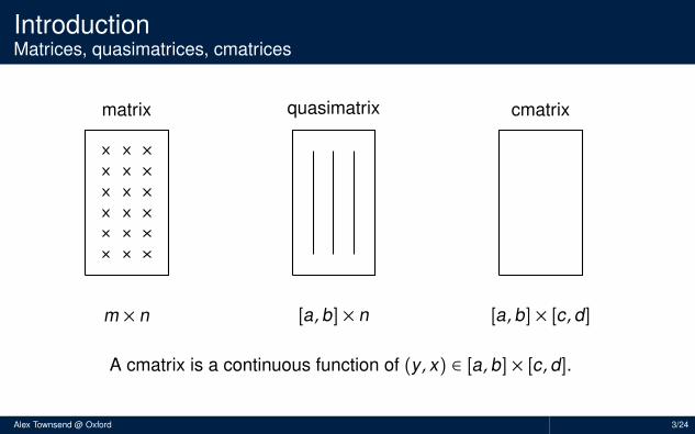
IntroductionMatrices, quasimatrices, cmatrices
..
matrix
.
quasimatrix
.
cmatrix
.
m × n
.
[a, b] × n
.
[a, b] × [c,d]
..................
A cmatrix is a continuous function of (y , x) ∈ [a, b] × [c,d].
Alex Townsend @ Oxford 3/24
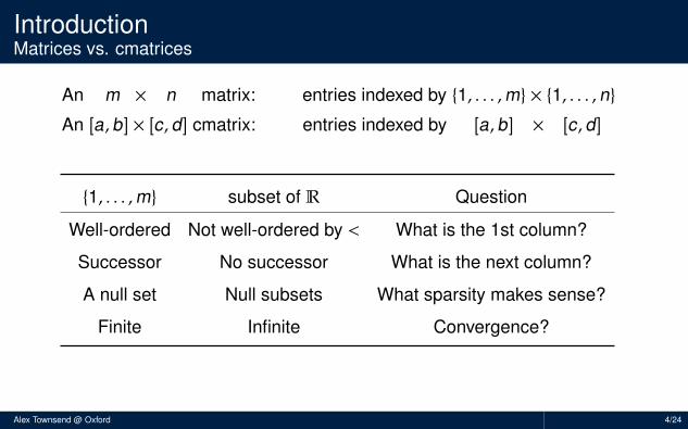
IntroductionMatrices vs. cmatrices
An m × n matrix: entries indexed by {1, . . . ,m} × {1, . . . , n}An [a,b] × [c, d] cmatrix: entries indexed by [a, b] × [c,d]
{1, . . . ,m} subset of R Question
Well-ordered Not well-ordered by < What is the 1st column?
Successor No successor What is the next column?
A null set Null subsets What sparsity makes sense?
Finite Infinite Convergence?
Three heroes: Smoothness pivoting εmach
Alex Townsend @ Oxford 4/24
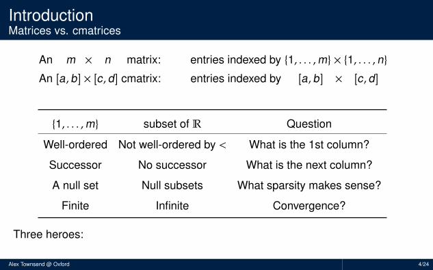
IntroductionMatrices vs. cmatrices
An m × n matrix: entries indexed by {1, . . . ,m} × {1, . . . , n}An [a,b] × [c, d] cmatrix: entries indexed by [a, b] × [c,d]
{1, . . . ,m} subset of R Question
Well-ordered Not well-ordered by < What is the 1st column?
Successor No successor What is the next column?
A null set Null subsets What sparsity makes sense?
Finite Infinite Convergence?
Three heroes:
Smoothness pivoting εmach
Alex Townsend @ Oxford 4/24
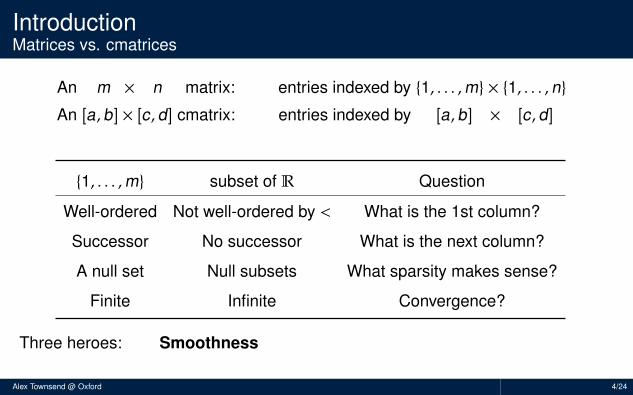
IntroductionMatrices vs. cmatrices
An m × n matrix: entries indexed by {1, . . . ,m} × {1, . . . , n}An [a,b] × [c, d] cmatrix: entries indexed by [a, b] × [c,d]
{1, . . . ,m} subset of R Question
Well-ordered Not well-ordered by < What is the 1st column?
Successor No successor What is the next column?
A null set Null subsets What sparsity makes sense?
Finite Infinite Convergence?
Three heroes: Smoothness
pivoting εmach
Alex Townsend @ Oxford 4/24

IntroductionMatrices vs. cmatrices
An m × n matrix: entries indexed by {1, . . . ,m} × {1, . . . , n}An [a,b] × [c, d] cmatrix: entries indexed by [a, b] × [c,d]
{1, . . . ,m} subset of R Question
Well-ordered Not well-ordered by < What is the 1st column?
Successor No successor What is the next column?
A null set Null subsets What sparsity makes sense?
Finite Infinite Convergence?
Three heroes: Smoothness pivoting
εmach
Alex Townsend @ Oxford 4/24
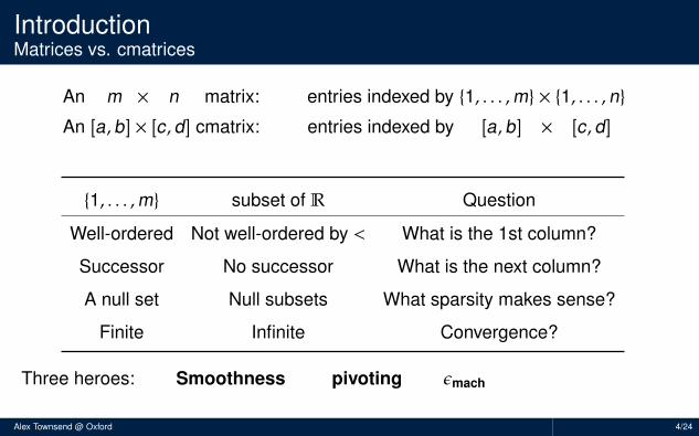
IntroductionMatrices vs. cmatrices
An m × n matrix: entries indexed by {1, . . . ,m} × {1, . . . , n}An [a,b] × [c, d] cmatrix: entries indexed by [a, b] × [c,d]
{1, . . . ,m} subset of R Question
Well-ordered Not well-ordered by < What is the 1st column?
Successor No successor What is the next column?
A null set Null subsets What sparsity makes sense?
Finite Infinite Convergence?
Three heroes: Smoothness pivoting εmach
Alex Townsend @ Oxford 4/24
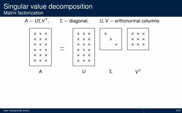
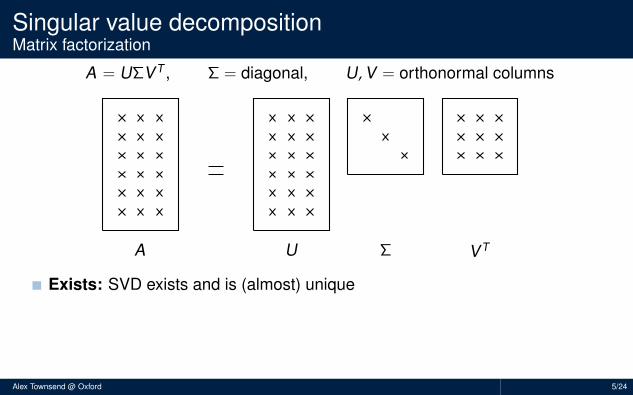
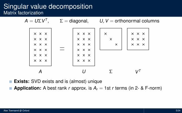
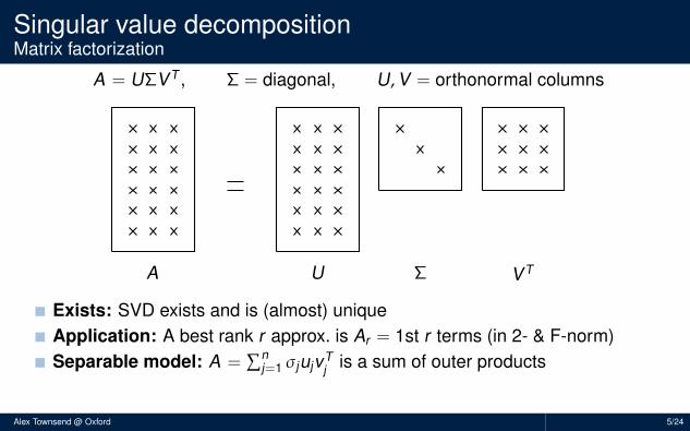
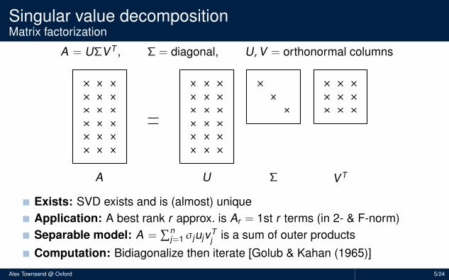
Singular value decompositionMatrix factorization
A = UΣVT , Σ = diagonal, U,V = orthonormal columns
..................................................A
.U
.Σ
.
VT
Exists: SVD exists and is (almost) uniqueApplication: A best rank r approx. is Ar = 1st r terms (in 2- & F-norm)Separable model: A =
∑nj=1 σjujvT
j is a sum of outer products
Computation: Bidiagonalize then iterate [Golub & Kahan (1965)]
Alex Townsend @ Oxford 5/24
Singular value decompositionMatrix factorization
A = UΣVT , Σ = diagonal, U,V = orthonormal columns
..................................................A
.U
.Σ
.
VT
Exists: SVD exists and is (almost) unique
Application: A best rank r approx. is Ar = 1st r terms (in 2- & F-norm)Separable model: A =
∑nj=1 σjujvT
j is a sum of outer products
Computation: Bidiagonalize then iterate [Golub & Kahan (1965)]
Alex Townsend @ Oxford 5/24
Singular value decompositionMatrix factorization
A = UΣVT , Σ = diagonal, U,V = orthonormal columns
..................................................A
.U
.Σ
.
VT
Exists: SVD exists and is (almost) uniqueApplication: A best rank r approx. is Ar = 1st r terms (in 2- & F-norm)
Separable model: A =∑n
j=1 σjujvTj is a sum of outer products
Computation: Bidiagonalize then iterate [Golub & Kahan (1965)]
Alex Townsend @ Oxford 5/24
Singular value decompositionMatrix factorization
A = UΣVT , Σ = diagonal, U,V = orthonormal columns
..................................................A
.U
.Σ
.
VT
Exists: SVD exists and is (almost) uniqueApplication: A best rank r approx. is Ar = 1st r terms (in 2- & F-norm)Separable model: A =
∑nj=1 σjujvT
j is a sum of outer products
Computation: Bidiagonalize then iterate [Golub & Kahan (1965)]
Alex Townsend @ Oxford 5/24
Singular value decompositionMatrix factorization
A = UΣVT , Σ = diagonal, U,V = orthonormal columns
..................................................A
.U
.Σ
.
VT
Exists: SVD exists and is (almost) uniqueApplication: A best rank r approx. is Ar = 1st r terms (in 2- & F-norm)Separable model: A =
∑nj=1 σjujvT
j is a sum of outer products
Computation: Bidiagonalize then iterate [Golub & Kahan (1965)]
Alex Townsend @ Oxford 5/24
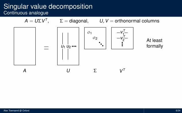
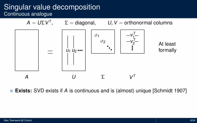
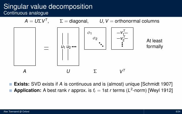
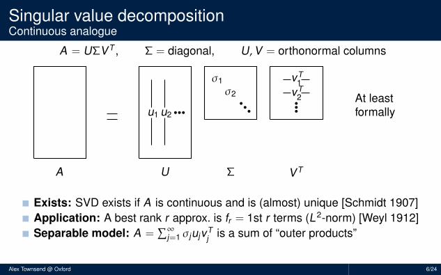
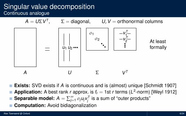
Singular value decompositionContinuous analogue
A = UΣVT , Σ = diagonal, U,V = orthonormal columns
..
u1
.
u2
....
σ1
.
σ2
....
vT2
.
vT1
....A
.U
.Σ
.
VT
.
At leastformally
Exists: SVD exists if A is continuous and is (almost) unique [Schmidt 1907]Application: A best rank r approx. is fr = 1st r terms (L2-norm) [Weyl 1912]Separable model: A =
∑∞j=1 σjujvT
j is a sum of “outer products”Computation: Avoid bidiagonalization
Alex Townsend @ Oxford 6/24
Singular value decompositionContinuous analogue
A = UΣVT , Σ = diagonal, U,V = orthonormal columns
..
u1
.
u2
....
σ1
.
σ2
....
vT2
.
vT1
....A
.U
.Σ
.
VT
.
At leastformally
Exists: SVD exists if A is continuous and is (almost) unique [Schmidt 1907]
Application: A best rank r approx. is fr = 1st r terms (L2-norm) [Weyl 1912]Separable model: A =
∑∞j=1 σjujvT
j is a sum of “outer products”Computation: Avoid bidiagonalization
Alex Townsend @ Oxford 6/24
Singular value decompositionContinuous analogue
A = UΣVT , Σ = diagonal, U,V = orthonormal columns
..
u1
.
u2
....
σ1
.
σ2
....
vT2
.
vT1
....A
.U
.Σ
.
VT
.
At leastformally
Exists: SVD exists if A is continuous and is (almost) unique [Schmidt 1907]Application: A best rank r approx. is fr = 1st r terms (L2-norm) [Weyl 1912]
Separable model: A =∑∞
j=1 σjujvTj is a sum of “outer products”
Computation: Avoid bidiagonalization
Alex Townsend @ Oxford 6/24
Singular value decompositionContinuous analogue
A = UΣVT , Σ = diagonal, U,V = orthonormal columns
..
u1
.
u2
....
σ1
.
σ2
....
vT2
.
vT1
....A
.U
.Σ
.
VT
.
At leastformally
Exists: SVD exists if A is continuous and is (almost) unique [Schmidt 1907]Application: A best rank r approx. is fr = 1st r terms (L2-norm) [Weyl 1912]Separable model: A =
∑∞j=1 σjujvT
j is a sum of “outer products”
Computation: Avoid bidiagonalization
Alex Townsend @ Oxford 6/24
Singular value decompositionContinuous analogue
A = UΣVT , Σ = diagonal, U,V = orthonormal columns
..
u1
.
u2
....
σ1
.
σ2
....
vT2
.
vT1
....A
.U
.Σ
.
VT
.
At leastformally
Exists: SVD exists if A is continuous and is (almost) unique [Schmidt 1907]Application: A best rank r approx. is fr = 1st r terms (L2-norm) [Weyl 1912]Separable model: A =
∑∞j=1 σjujvT
j is a sum of “outer products”Computation: Avoid bidiagonalization
Alex Townsend @ Oxford 6/24
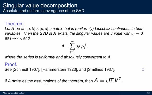
Singular value decompositionAbsolute and uniform convergence of the SVD
TheoremLet A be an [a,b] × [c, d] cmatrix that is (uniformly) Lipschitz continuous in bothvariables. Then the SVD of A exists, the singular values are unique with σj → 0as j →∞, and
A =
∞∑j=1
σjujvTj ,
where the series is uniformly and absolutely convergent to A.
Proof.See [Schmidt 1907], [Hammerstein 1923], and [Smithies 1937]. �
If A satisfies the assumptions of the theorem, then A = UΣVT .
Alex Townsend @ Oxford 7/24
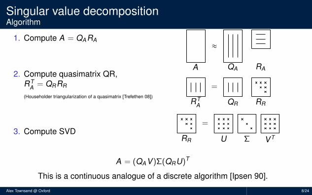
Singular value decompositionAlgorithm
1. Compute A = QARA
2. Compute quasimatrix QR,RT
A = QRRR
(Householder triangularization of a quasimatrix [Trefethen 08])
3. Compute SVD
..
≈.
A.
QA.
RA
..=
.......RT
A
.QR
.RR
........=
......................RR
.U
.Σ
.VT
A = (QAV)Σ(QRU)T
This is a continuous analogue of a discrete algorithm [Ipsen 90].
Alex Townsend @ Oxford 8/24
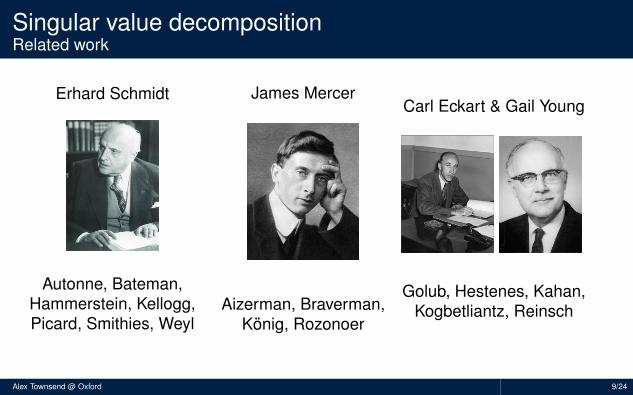
Singular value decompositionRelated work
Erhard Schmidt
Autonne, Bateman,Hammerstein, Kellogg,Picard, Smithies, Weyl
James Mercer
Aizerman, Braverman,Konig, Rozonoer
Carl Eckart & Gail Young
Golub, Hestenes, Kahan,Kogbetliantz, Reinsch
Alex Townsend @ Oxford 9/24
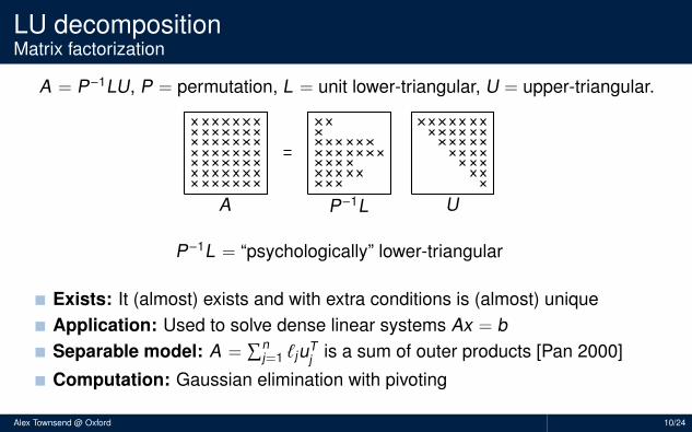
LU decompositionMatrix factorization
A = P−1LU, P = permutation, L = unit lower-triangular, U = upper-triangular.
..A
.P−1L
.U
.........................................................................................................
P−1L = “psychologically” lower-triangular
Exists: It (almost) exists and with extra conditions is (almost) uniqueApplication: Used to solve dense linear systems Ax = bSeparable model: A =
∑nj=1 `juT
j is a sum of outer products [Pan 2000]
Computation: Gaussian elimination with pivoting
Alex Townsend @ Oxford 10/24
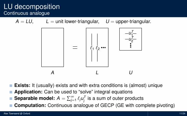
LU decompositionContinuous analogue
A = LU, L = unit lower-triangular, U = upper-triangular.
..
`1
.
`2
....
uT1
.
uT2
....A
.L
.U
Exists: It (usually) exists and with extra conditions is (almost) uniqueApplication: Can be used to “solve” integral equationsSeparable model: A =
∑∞j=1 `juT
j is a sum of outer productsComputation: Continuous analogue of GECP (GE with complete pivoting)
Alex Townsend @ Oxford 11/24
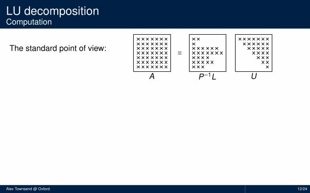
LU decompositionComputation
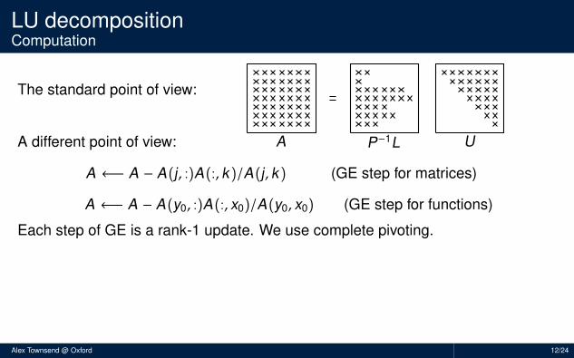
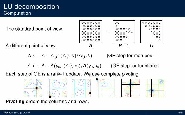
The standard point of view:
A different point of view:
..A
.P−1L
.U
.........................................................................................................
A ←− A − A(j, :)A(:, k )/A(j, k ) (GE step for matrices)
A ←− A − A(y0, :)A(:, x0)/A(y0, x0) (GE step for functions)
Each step of GE is a rank-1 update. We use complete pivoting.
Pivoting orders the columns and rows.
Alex Townsend @ Oxford 12/24
LU decompositionComputation
The standard point of view:
A different point of view:..
A.
P−1L.
U.........................................................................................................
A ←− A − A(j, :)A(:, k )/A(j, k ) (GE step for matrices)
A ←− A − A(y0, :)A(:, x0)/A(y0, x0) (GE step for functions)
Each step of GE is a rank-1 update. We use complete pivoting.
Pivoting orders the columns and rows.
Alex Townsend @ Oxford 12/24

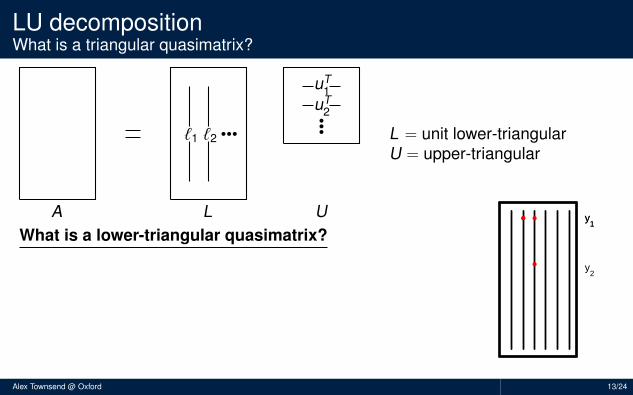
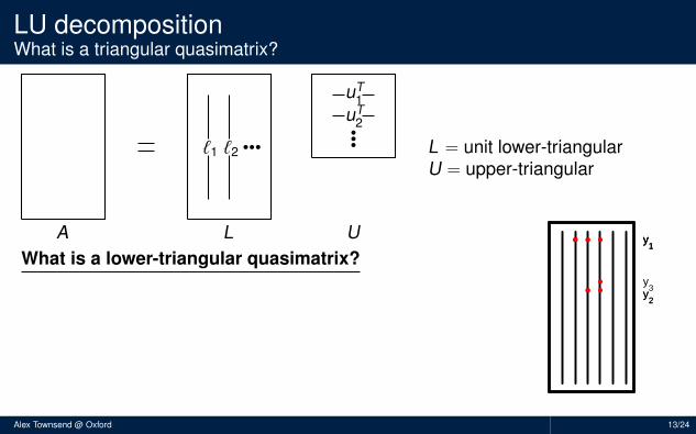
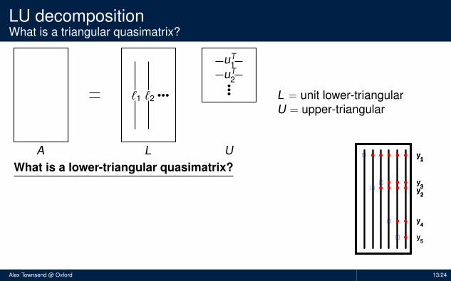
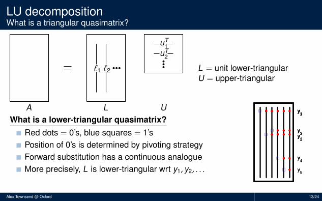
LU decompositionWhat is a triangular quasimatrix?
..
`1
.
`2
....
uT1
.
uT2
....A
.L
.U
L = unit lower-triangularU = upper-triangular
What is a lower-triangular quasimatrix?
Red dots = 0’s, blue squares = 1’sPosition of 0’s is determined by pivoting strategyForward substitution has a continuous analogueMore precisely, L is lower-triangular wrt y1, y2, . . .
Alex Townsend @ Oxford 13/24

LU decompositionWhat is a triangular quasimatrix?
..
`1
.
`2
....
uT1
.
uT2
....A
.L
.U
L = unit lower-triangularU = upper-triangular
What is a lower-triangular quasimatrix?
Red dots = 0’s, blue squares = 1’sPosition of 0’s is determined by pivoting strategyForward substitution has a continuous analogueMore precisely, L is lower-triangular wrt y1, y2, . . .
y1
Alex Townsend @ Oxford 13/24
LU decompositionWhat is a triangular quasimatrix?
..
`1
.
`2
....
uT1
.
uT2
....A
.L
.U
L = unit lower-triangularU = upper-triangular
What is a lower-triangular quasimatrix?
Red dots = 0’s, blue squares = 1’sPosition of 0’s is determined by pivoting strategyForward substitution has a continuous analogueMore precisely, L is lower-triangular wrt y1, y2, . . .
y1
y1
y2
y1
y2
y3
Alex Townsend @ Oxford 13/24

LU decompositionWhat is a triangular quasimatrix?
..
`1
.
`2
....
uT1
.
uT2
....A
.L
.U
L = unit lower-triangularU = upper-triangular
What is a lower-triangular quasimatrix?
Red dots = 0’s, blue squares = 1’sPosition of 0’s is determined by pivoting strategyForward substitution has a continuous analogueMore precisely, L is lower-triangular wrt y1, y2, . . .
y1
y1
y2
y1
y2
y3
y1
y2
y3
y4
y1
y2
y3
y4
y5
Alex Townsend @ Oxford 13/24
LU decompositionWhat is a triangular quasimatrix?
..
`1
.
`2
....
uT1
.
uT2
....A
.L
.U
L = unit lower-triangularU = upper-triangular
What is a lower-triangular quasimatrix?
Red dots = 0’s, blue squares = 1’sPosition of 0’s is determined by pivoting strategyForward substitution has a continuous analogueMore precisely, L is lower-triangular wrt y1, y2, . . .
y1
y1
y2
y1
y2
y3
y1
y2
y3
y4
y1
y2
y3
y4
y5
y1
y2
y3
y4
y5
Alex Townsend @ Oxford 13/24
LU decompositionWhat is a triangular quasimatrix?
..
`1
.
`2
....
uT1
.
uT2
....A
.L
.U
L = unit lower-triangularU = upper-triangular
What is a lower-triangular quasimatrix?Red dots = 0’s, blue squares = 1’sPosition of 0’s is determined by pivoting strategyForward substitution has a continuous analogueMore precisely, L is lower-triangular wrt y1, y2, . . .
y1
y1
y2
y1
y2
y3
y1
y2
y3
y4
y1
y2
y3
y4
y5
y1
y2
y3
y4
y5
Alex Townsend @ Oxford 13/24
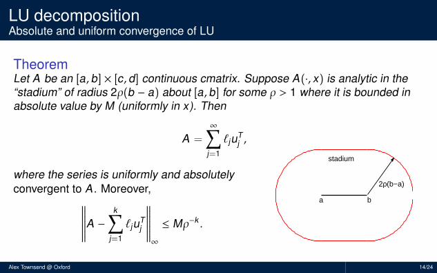
LU decompositionAbsolute and uniform convergence of LU
TheoremLet A be an [a,b] × [c, d] continuous cmatrix. Suppose A(·, x) is analytic in the“stadium” of radius 2ρ(b − a) about [a, b] for some ρ > 1 where it is bounded inabsolute value by M (uniformly in x). Then
A =
∞∑j=1
`juTj ,
where the series is uniformly and absolutelyconvergent to A. Moreover,∥∥∥∥∥∥∥A −
k∑j=1
`juTj
∥∥∥∥∥∥∥∞
≤ Mρ−k .
a b
2ρ(b−a)
stadium
Alex Townsend @ Oxford 14/24
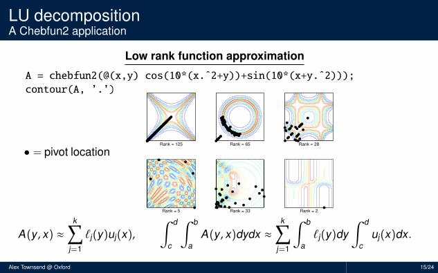
LU decompositionA Chebfun2 application
Low rank function approximation
A = chebfun2(@(x,y) cos(10*(x.ˆ2+y))+sin(10*(x+y.ˆ2)));
contour(A, ’.’)
• = pivot locationRank = 125 Rank = 65 Rank = 28
Rank = 5 Rank = 33 Rank = 2
A(y , x) ≈k∑
j=1
`j(y)uj(x),∫ d
c
∫ b
aA(y , x)dydx ≈
k∑j=1
∫ b
a`j(y)dy
∫ d
cuj(x)dx .
Alex Townsend @ Oxford 15/24
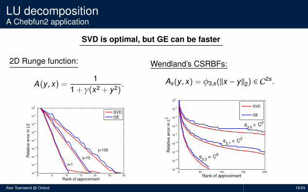
LU decompositionA Chebfun2 application
SVD is optimal, but GE can be faster
2D Runge function:
A(y , x) =1
1 + γ(x2 + y2).
0 5 10 15 20 25 3010
−16
10−14
10−12
10−10
10−8
10−6
10−4
10−2
100
Rank of approximant
Rela
tive e
rror
in L
2
SVD
GE
γ=1
γ=10
γ=100
Wendland’s CSRBFs:
As(y , x) = φ3,s(‖x − y‖2) ∈ C2s .
0 50 100 150 20010
−16
10−14
10−12
10−10
10−8
10−6
10−4
10−2
100
Rank of approximant
Re
lative
err
or
in L
2
SVD
GE
φ3,1
∈ C2
φ3,3
∈ C6
φ3,0
∈ C0
Alex Townsend @ Oxford 16/24

LU decompositionRelated work
Eugene Tyrtyshnikov
Goreinov, Oseledets,Savostyanov,Zamarashkin
Mario Bebendorf
Gesenhues, Griebel,Hackbusch, Rjasanow
Keith Geddes
Carvajal, Chapman
Petros Drineas
Candes, Greengard,Mahoney, Martinsson,
Rokhlin
Moral of the story: Iterative GE is everywhere, under different guises
Many others: Halko, Liberty, Martinsson, O’Neil, Tropp, Tygert, Woolfe, etc.
Alex Townsend @ Oxford 17/24
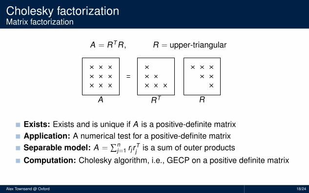
Cholesky factorizationMatrix factorization
A = RTR, R = upper-triangular
..A
.RT
.R
.....................
Exists: Exists and is unique if A is a positive-definite matrixApplication: A numerical test for a positive-definite matrixSeparable model: A =
∑nj=1 rjrT
j is a sum of outer products
Computation: Cholesky algorithm, i.e., GECP on a positive definite matrix
Alex Townsend @ Oxford 18/24
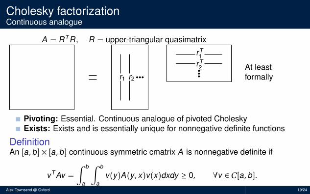
Cholesky factorizationContinuous analogue
A = RTR, R = upper-triangular quasimatrix
..
r1
.
r2
.......
rT1
.
rT2
.
At leastformally
Pivoting: Essential. Continuous analogue of pivoted CholeskyExists: Exists and is essentially unique for nonnegative definite functions
DefinitionAn [a,b] × [a,b] continuous symmetric cmatrix A is nonnegative definite if
vTAv =
∫ b
a
∫ b
av(y)A(y , x)v(x)dxdy ≥ 0, ∀v ∈ C[a,b].
Alex Townsend @ Oxford 19/24
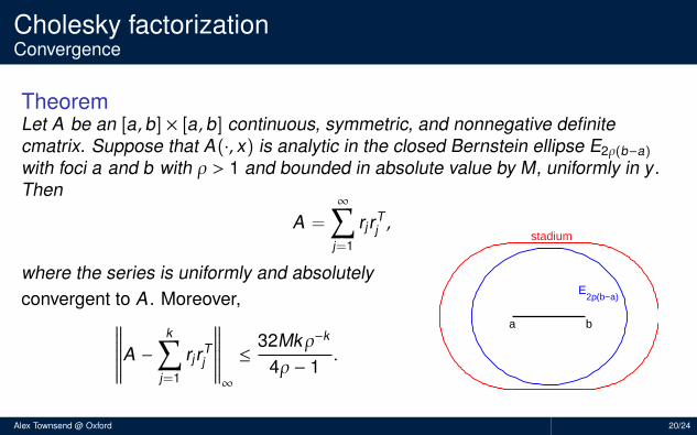
Cholesky factorizationConvergence
TheoremLet A be an [a,b] × [a,b] continuous, symmetric, and nonnegative definitecmatrix. Suppose that A(·, x) is analytic in the closed Bernstein ellipse E2ρ(b−a)with foci a and b with ρ > 1 and bounded in absolute value by M, uniformly in y.Then
A =
∞∑j=1
rjrTj ,
where the series is uniformly and absolutelyconvergent to A. Moreover,∥∥∥∥∥∥∥A −
k∑j=1
rjrTj
∥∥∥∥∥∥∥∞
≤32Mkρ−k
4ρ − 1.
a b
stadium
E2ρ(b−a)
Alex Townsend @ Oxford 20/24
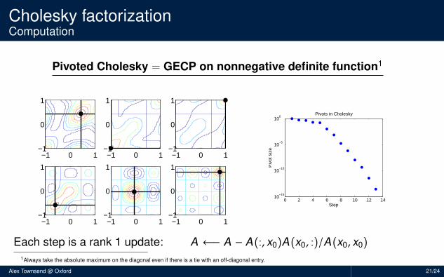
Cholesky factorizationComputation
Pivoted Cholesky = GECP on nonnegative definite function1
−1 0 1−1
0
1
−1 0 1−1
0
1
−1 0 1−1
0
1
−1 0 1−1
0
1
−1 0 1−1
0
1
−1 0 1−1
0
1
0 2 4 6 8 10 12 1410
−15
10−10
10−5
100
Step
Piv
ot s
ize
Pivots in Cholesky
Each step is a rank 1 update: A ←− A − A(:, x0)A(x0, :)/A(x0, x0)1Always take the absolute maximum on the diagonal even if there is a tie with an off-diagonal entry.
Alex Townsend @ Oxford 21/24
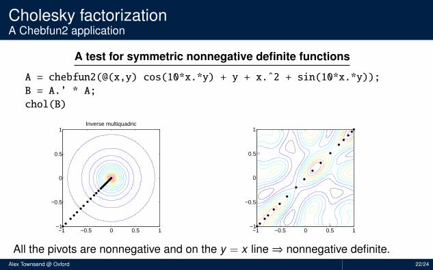
Cholesky factorizationA Chebfun2 application
A test for symmetric nonnegative definite functions
A = chebfun2(@(x,y) cos(10*x.*y) + y + x.ˆ2 + sin(10*x.*y));
B = A.’ * A;
chol(B)
Inverse multiquadric
−1 −0.5 0 0.5 1−1
−0.5
0
0.5
1
−1 −0.5 0 0.5 1−1
−0.5
0
0.5
1
All the pivots are nonnegative and on the y = x line⇒ nonnegative definite.Alex Townsend @ Oxford 22/24

Demo
Demo
Alex Townsend @ Oxford 23/24
References
Z. Battles & L. N. Trefethen, An extension of MATLAB to continuous functions and operators, SISC, 25 (2004),pp. 1743–1770.
T. A. Driscoll, F. Bornemann, & L. N. Trefethen, The chebop system for automatic solution of differentialequations, BIT, 48 (2008), pp. 701–723.
C. Eckart & G. Young, The approximation of one matrix by another of lower rank, Psychometrika, 1 (1936),pp. 211–218.
N. J. Higham, Accuracy and Stability of Numerical Algorithms, 2nd edition, SIAM, 2002.
E. Schmidt, Zur Theorie der linearen und nichtlinearen Integralgleichungen. I Teil. Entwicklung willkurlichenFunktionen nach System vorgeschriebener, Math. Ann., 63 (1907), pp. 433–476.
G. W. Stewart, Afternotes Goes to Graduate School, Philadelphia, SIAM, 1998.
T. & L. N. Trefethen, Gaussian elimination as an iterative algorithm, SIAM News, March 2013.
T. & L. N. Trefethen, An extension of Chebfun to two dimensions, to appear in SISC, 2013.
Alex Townsend @ Oxford 24/24