1

Paper 288-2017

Continuous Predictors in Regression Analyses Ruth Croxford, Institute for Clinical Evaluative Sciences, Toronto, Ontario, Canada

ABSTRACT

This presentation discusses the options for including continuous covariates in regression models. In his book, Clinical Prediction Models, Ewout Steyerberg presents a hierarchy of procedures for continuous predictors, starting with dichotomizing the variable and moving to modeling the variable using restricted cubic splines or using a fractional polynomial model. This presentation discusses all of the choices, with a focus on the last two. Restricted cubic splines express the relationship between the continuous covariate and the outcome using a set of cubic polynomials, which are constrained to meet at pre-specified points, called knots. Between the knots, each curve can take on the shape that best describes the data. A fractional polynomial model is another flexible method for modeling a relationship that is possibly nonlinear. In this model, polynomials with noninteger and negative powers are considered, along with the more conventional square and cubic polynomials, and the small subset of powers that best fits the data is selected. The presentation describes and illustrates these methods at an introductory level intended to be useful to anyone who is familiar with regression analyses.

INTRODUCTION There are two reasons to include a continuous independent variable in a regression model. First, the continuous variable may be the risk factor we’re interested in. For example, we may be interested in the role of surgeon experience on the probability of complications during surgery, and we want to do a good job of capturing the shape of the relationship between this risk factor and the outcome. Or the continuous variable is a confounder – a variable that we want to adjust for before looking at the impact of the risk factor of interest. For example, we may want to adjust properly for the effect of age or socioeconomic status before looking at the effect of treatment. Whatever the motivation, it is important to correctly identify the form of the relationship between the continuous predictor and the outcome variable. Failure to do so can result in a reduction in power, failure to identify an important relationship, and over or underestimation of the effect of a predictor.

The goal of this paper is to give an overview of the ways in which continuous predictors can be incorporated into regression models. The focus is on two approaches which can easily be used to test for and characterize non-linear relationships between continuous independent variables and the outcome: restricted cubic splines and fractional polynomials. Because the methods are functions only of the continuous independent variables, they can be applied to any regression, regardless of the nature of the outcome variable.

INCORPORATING CONTINUOUS INDEPENDENT VARIABLES INTO REGRESSION MODELS In his book Clinical Prediction Models, Steyerberg summarizes the ways in which continuous predictors can be incorporated into a regression model. (Steyerberg, 2009) His hierarchy is shown in Table 1. While the focus of this paper is on restricted cubic splines and fractional polynomials, I will spend some time discussing some of the other choices, in order to introduce some precautionary notes as well as some of the considerations mentioned in the section on restricted cubic splines.

2

Procedure Characteristics Recommendation Dichotomization Simple, easy interpretation Bad idea More categories Categories capture prognostic information better,

but are not smooth; sensitive to choice of cut-points and hence instable

Primarily for illustration, comparison with published evidence

Linear Simple Often reasonable as a start Transformations Log, square root, inverse, exponent, etc. May provide robust summaries

of non-linearity Restricted cubic splines

Flexible functions with robust behaviour at the tails of predictor distributions

Flexible descriptions of non-linearity

Fractional polynomials

Flexible combinations of polynomials; behaviour in the tails may be unstable

Flexible descriptions of non-linearity

Table 1. Options for including continuous predictors in a regression analysis (adapted from Steyerberg (2009), Clinical Prediction Models

DICHOTOMIZATION Dichotomization of continuous predictors is commonly used in health services research, so it is worth spending a bit of time looking at it. When continuous predictors are dichotomized, the regression results are easy to interpret, are consistent with the goal of making yes/no decisions in clinical practice (e.g., to treat or not to treat), and tend to be aligned with how we simplify a complex world (e.g., hospitals are either high volume or low volume, individuals either have diabetes or do not, place of residence is either urban or rural). However, it is important to understand the drawbacks associated with dichotomization.

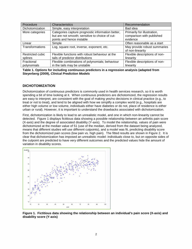
First, dichotomization is likely to lead to an unrealistic model, and one in which non-linearity cannot be detected. Figure 1 displays fictitious data showing a possible relationship between an arthritis pain score (X-axis) and the degree of associated disability (Y-axis). To model the relationship, values of pain were dichotomized at the median value of 51 (use of the median, derived from the dataset being analyzed, means that different studies will use different cutpoints), and a model was fit, predicting disability score from the dichotomized pain scores (low pain vs. high pain). The fitted results are shown in Figure 2. It is clear that dichotomization has imposed an unrealistic model: individuals close to, but on opposite sides of the cutpoint are predicted to have very different outcomes and the predicted values hide the amount of variation in disability scores.

Figure 1. Fictitious data showing the relationship between an individual's pain score (X-axis) and disability score (Y-axis)

3

Figure 2. Predicted disabilty scores (red lines) based on a model in which pain score was dichotomized using a cutpoint at the median value. When the dichotomized continuous variable is the risk factor of interest, dichotomization leads to a large loss of power, leading to failure to identify an association and increasing the probability of a false negative result. Dichotomizing a normally distributed continuous variable is equivalent, in loss of power, to decreasing the sample size by a third; for exponentially distributed variables the impact is larger. (Royston, Altman and Sauerbrei, 2006) Furthermore, the choice of cutpoint is problematic. When there is no theoretical basis for the cutpoint, it is often chosen as a quantile of the data being analyzed, so that different studies use different categories. Another approach is to search for the “best” cutpoint, an approach that results in muiltiple testing and an overestimation of the treatment effect (and inflation of the type I error rate).

Conversely, dichotomizing a confounder increases the probability of incorrectly identifying as association between a continuous risk factor and the outcome, increasing the probability of a false positive result. (Austin and Brunner, 2004) The inflation in the type I error rate (the probability of incorrectly concluding that there is an association between the risk factor and the outcome) increases with sample size and with the degree of correlation between the confounder and the risk factor, and decreases, but does not disappear, with an increase in the number of categories.

Creating multiple categories provides more flexibility, although information is still lost, the results can still be misleading and are dependent on the choice of categories. Nevertheless, as Steyerberg noted (Table 1) categorization can be useful, particularly when the goal is to compare results with previously published reports.

When categorization is desired for ease of model interpretation, the recommendation is to model continuous predictors as continuous in order to arrive at a model, and then later to categorize them into risk groups in such a way as to capture the results.

LINEAR RELATIONSHIP Often, a linear model provides a good fit to the data. Certainly, as shown in Figure 3. Predicted disabilty scores (red line) based on a model in which pain score is linearly related to disability., a straight line happens to capture the relationship between pain and disability in the example dataset fairly well. The linear model fails to capture the relationship between pain and disability for very low and very high values of pain. Whether this is good enough depends on the goal of the model.

4

Figure 3. Predicted disabilty scores (red line) based on a model in which pain score is linearly related to disability. A linear relationship should be tested, not assumed. The sections on restricted cubic splines and fractional polynomials below offer straightforward tests for the adequacy of a linear model.

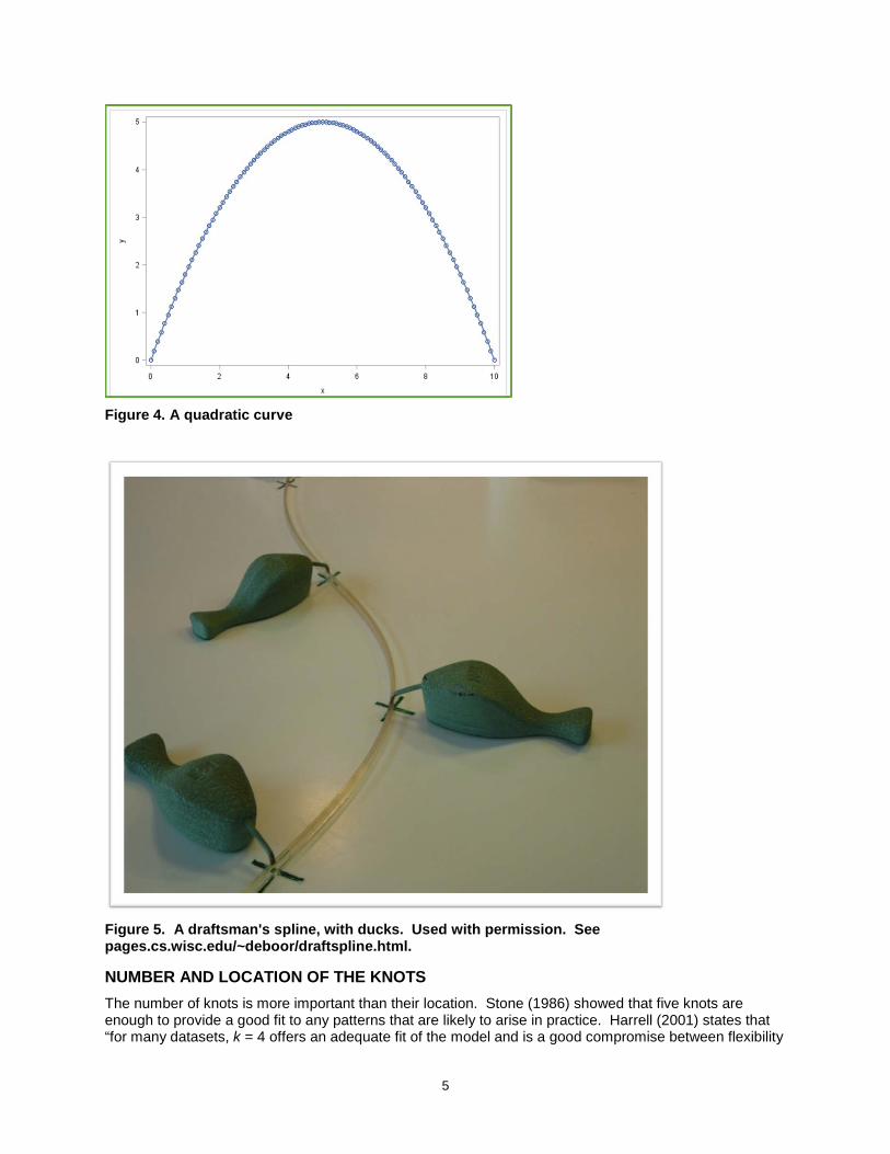
POLYNOMIALS As is the case with the example dataset, the relationship between a continuous predictor and the outcome variable is often curved. When we suspect there may be a non-linear relationship between predictor and outcome, we generally use a polynomial, and generally restrict our exploration to the addition of a quadratic term. Figure 4 shows a quadratic curve, simply to illustrate two limitations to polynomials. The first is that lower order polynomials offer a limited number of shapes – a quadratic predictor is limited to modeling U and inverted-U relationships. The second is that what goes up must come back down again, at the same rate that it went up (or, in the case of an inverted-U relationship, what goes down must come back up). This means that polynomials cannot capture asymptotes: the fitted curve must start to curve back down, even if the data flatten out. Therefore, polynomials tend to fit the data poorly at the extreme ends, a consideration which will be discussed again in the context of restricted cubic splines.

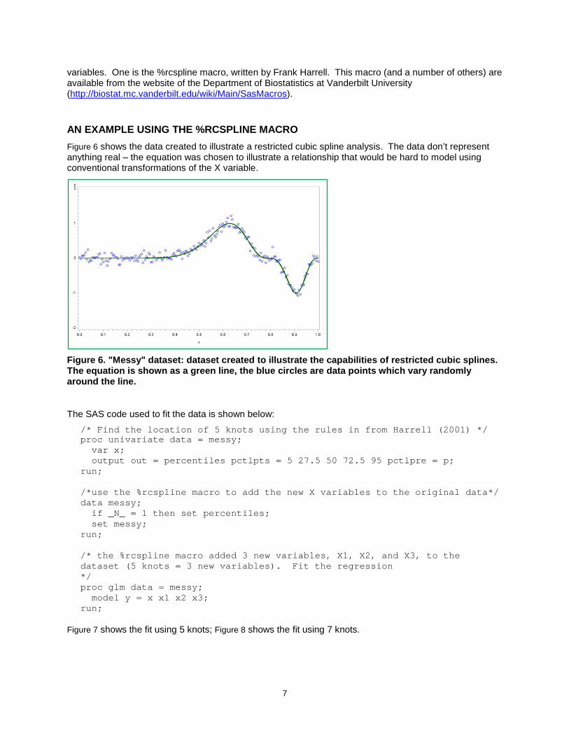
RESTRICTED CUBIC SPLINES Figure 5 is a photograph of a draftman’s spline. Originally used to design boats, a drafting spline consists of a flexible strip held in place at specific locations by weights called ducks (because their shape supposedly resembles a duck). The ducks force the spline to pass through selected points, called knots. Between those points, the strip is free to follow the curve of least resistance. Individual curves join together smoothly where they meet at the knots.

Splines used to model the relationship between a continuous predictor and an outcome are analogous to the physical spline shown in Figure 5. The range of the predictor values is divided into segments using a set of knots. Separate regression curves are fit to the data between the knots in such a way that the individual curves are forced to join “smoothly” at the knots. “Smoothly joined” means that for polynomials of degree n, both the spline function and its first n-1 derivatives are continuous at the knots.

5

Figure 4. A quadratic curve

Figure 5. A draftsman's spline, with ducks. Used with permission. See pages.cs.wisc.edu/~deboor/draftspline.html.

NUMBER AND LOCATION OF THE KNOTS The number of knots is more important than their location. Stone (1986) showed that five knots are enough to provide a good fit to any patterns that are likely to arise in practice. Harrell (2001) states that “for many datasets, k = 4 offers an adequate fit of the model and is a good compromise between flexibility

6

and loss of precision caused by overfitting a small sample”. If the sample size is small, three knots should be used in order to have enough observations in between the knots to be able to fit each polynomial. If the sample size is large and if there is reason to believe that the relationship being studied changes quickly, more than five knots can be used.

For some studies, theory may suggest the location of the knots. More commonly, the location of the knots are prespecified based on the quantiles of the continuous variable. This ensures that there are enough observations in each interval to estimate the cubic polynomial. Table 2, from Harrell (2001) shows suggested locations for the knots.

Number of knots

(K)

Knot locations expressed in quantiles of the X variable

3 0.1 0.5 0.9

4 0.5 0.35 0.65 0.95

5 0.5 0.275 0.5 0.725 0.95

6 0.5 0.23 0.41 0.59 0.77 0.95

7 0.025 0.1833 0.3417 0.5 0.6583 0.8167 0.975

Table 2. Location of knots. From Harrell (2001)

DEFINING THE SPLINES In practice, as the name ‘cubic splines’ indicates, cubic polynomials are used to model the curves between the knots. Cubic polynomials are chosen because this is the smallest degree of polynomial that allows an inflection, thereby providing flexibility while minimizing the degrees of freedom required. Because cubic splines tend to fit poorly at the two tails (before the first knot and after the last knot), restricted cubic splines are used: the splines are constrained to be linear in the two tails, providing a better fit to the data. Therefore, in order to model a continuous variable using restricted cubic splines, a set of k-2 new variables are calculated; these new variables are transformations of the original continuous predictor:

Let u+ = u if u > 0

u+ = 0 if u ≤ 0

If the k knots are placed at t1 < t2< . . . < tk, then for continuous variable x, the k-2 new variables are defined as:

𝑥𝑥𝑖𝑖 = (𝑥𝑥 − 𝑡𝑡𝑖𝑖)+3 − (𝑥𝑥 − 𝑡𝑡𝑘𝑘−1)+3 𝑡𝑡𝑘𝑘 − 𝑡𝑡𝑖𝑖𝑡𝑡𝑘𝑘 − 𝑡𝑡𝑘𝑘−1

+ (𝑥𝑥 − 𝑡𝑡𝑘𝑘)+3 𝑡𝑡𝑘𝑘−1 − 𝑡𝑡𝑖𝑖𝑡𝑡𝑘𝑘 − 𝑡𝑡𝑘𝑘−1

, 𝑖𝑖 = 1, . . , 𝑘𝑘 − 2

Thus, the original continuous predictor has been augmented with the addition of new variables which have been defined in such a way that the curves will meet at the knots. The regression model can now be fit using the usual regression procedures, and inferences can be drawn as usual. In particular, we can test for non-linearity by comparing the log-likelihood of the model containing the new variables with the log-likelihood of a model containing x as a linear variable. Fitting a continuous variable using restricted cubic splines in a regression analysis uses k – 1 degrees of freedom (the original linear variable X plus the k – 2 piecewise cubic variables) in addition to the intercept.

THERE’S A MACRO Both the LOGISTIC and PHREG procedures now implement restricted cubic spline models via the EFFECT statement. Additionally, a number of people have written SAS® macros to calculate the required

7

variables. One is the %rcspline macro, written by Frank Harrell. This macro (and a number of others) are available from the website of the Department of Biostatistics at Vanderbilt University (http://biostat.mc.vanderbilt.edu/wiki/Main/SasMacros).

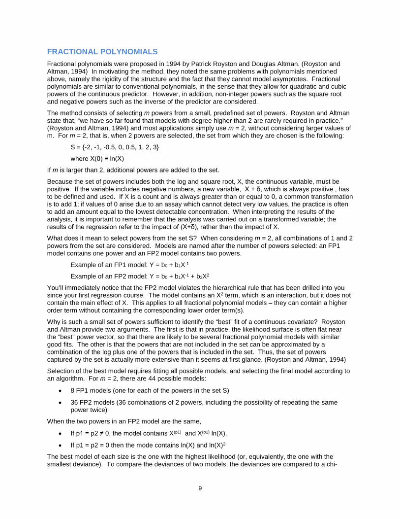
AN EXAMPLE USING THE %RCSPLINE MACRO Figure 6 shows the data created to illustrate a restricted cubic spline analysis. The data don’t represent anything real – the equation was chosen to illustrate a relationship that would be hard to model using conventional transformations of the X variable.

Figure 6. "Messy" dataset: dataset created to illustrate the capabilities of restricted cubic splines. The equation is shown as a green line, the blue circles are data points which vary randomly around the line.

The SAS code used to fit the data is shown below: /* Find the location of 5 knots using the rules in from Harrell (2001) */ proc univariate data = messy; var x; output out = percentiles pctlpts = 5 27.5 50 72.5 95 pctlpre = p; run; /*use the %rcspline macro to add the new X variables to the original data*/ data messy; if _N_ = 1 then set percentiles; set messy; run; /* the %rcspline macro added 3 new variables, X1, X2, and X3, to the dataset (5 knots = 3 new variables). Fit the regression */ proc glm data = messy; model y = x x1 x2 x3; run;

Figure 7 shows the fit using 5 knots; Figure 8 shows the fit using 7 knots.

8

Figure 7. Regression line fit to the "messy" data using restricted cubic splines with 5 knots

Figure 8. Regression line fit to the "messy" data using restricted cubic splines with 7 knots

Summary, RCS In summary, restricted cubic splines augment the original continuous predictor, adding a set of new variables. The regression model can then be fit using the usual regression procedures, and inferences can be drawn as usual. In particular, a test of non-linearity can easily be performed by comparing the spline model to a linear model. Since the new variables are simply a restatement of the original predictor, restricted cubic splines can be used in any type of regression.

In addition to the fact that new predictors have been added – a problem for small datasets – the main drawback to the method is the difficulty in presenting and interpreting the results. A graphical presentation is likely to be the most useful way to illustrate the relationship between predictor and outcome.

9

FRACTIONAL POLYNOMIALS Fractional polynomials were proposed in 1994 by Patrick Royston and Douglas Altman. (Royston and Altman, 1994) In motivating the method, they noted the same problems with polynomials mentioned above, namely the rigidity of the structure and the fact that they cannot model asymptotes. Fractional polynomials are similar to conventional polynomials, in the sense that they allow for quadratic and cubic powers of the continuous predictor. However, in addition, non-integer powers such as the square root and negative powers such as the inverse of the predictor are considered.

The method consists of selecting m powers from a small, predefined set of powers. Royston and Altman state that, “we have so far found that models with degree higher than 2 are rarely required in practice.” (Royston and Altman, 1994) and most applications simply use m = 2, without considering larger values of m. For m = 2, that is, when 2 powers are selected, the set from which they are chosen is the following:

S = {-2, -1, -0.5, 0, 0.5, 1, 2, 3}

where X(0) ≡ ln(X)

If m is larger than 2, additional powers are added to the set.

Because the set of powers includes both the log and square root, X, the continuous variable, must be positive. If the variable includes negative numbers, a new variable, X + δ, which is always positive , has to be defined and used. If X is a count and is always greater than or equal to 0, a common transformation is to add 1; if values of 0 arise due to an assay which cannot detect very low values, the practice is often to add an amount equal to the lowest detectable concentration. When interpreting the results of the analysis, it is important to remember that the analysis was carried out on a transformed variable; the results of the regression refer to the impact of (X+δ), rather than the impact of X.

What does it mean to select powers from the set S? When considering m = 2, all combinations of 1 and 2 powers from the set are considered. Models are named after the number of powers selected: an FP1 model contains one power and an FP2 model contains two powers.

Example of an FP1 model: Y = b0 + b1X-1

Example of an FP2 model: Y = b0 + b1X-1 + b2X2

You’ll immediately notice that the FP2 model violates the hierarchical rule that has been drilled into you since your first regression course. The model contains an X2 term, which is an interaction, but it does not contain the main effect of X. This applies to all fractional polynomial models – they can contain a higher order term without containing the corresponding lower order term(s).

Why is such a small set of powers sufficient to identify the “best” fit of a continuous covariate? Royston and Altman provide two arguments. The first is that in practice, the likelihood surface is often flat near the “best” power vector, so that there are likely to be several fractional polynomial models with similar good fits. The other is that the powers that are not included in the set can be approximated by a combination of the log plus one of the powers that is included in the set. Thus, the set of powers captured by the set is actually more extensive than it seems at first glance. (Royston and Altman, 1994)

Selection of the best model requires fitting all possible models, and selecting the final model according to an algorithm. For m = 2, there are 44 possible models:

• 8 FP1 models (one for each of the powers in the set S)

• 36 FP2 models (36 combinations of 2 powers, including the possibility of repeating the same power twice)

When the two powers in an FP2 model are the same,

• If p1 = p2 ≠ 0, the model contains X(p1) and X(p1) ln(X).

• If p1 = p2 = 0 then the mode contains ln(X) and ln(X)2.

The best model of each size is the one with the highest likelihood (or, equivalently, the one with the smallest deviance). To compare the deviances of two models, the deviances are compared to a chi-

10

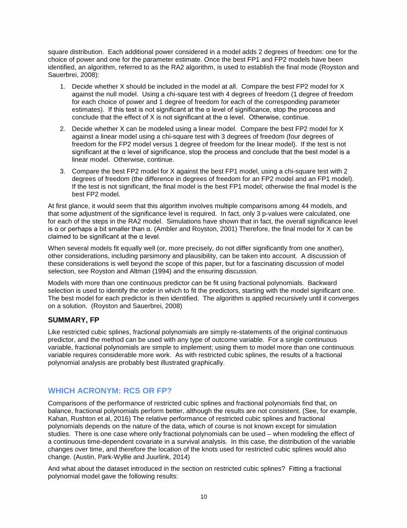
square distribution. Each additional power considered in a model adds 2 degrees of freedom: one for the choice of power and one for the parameter estimate. Once the best FP1 and FP2 models have been identified, an algorithm, referred to as the RA2 algorithm, is used to establish the final mode (Royston and Sauerbrei, 2008):

1. Decide whether X should be included in the model at all. Compare the best FP2 model for X against the null model. Using a chi-square test with 4 degrees of freedom (1 degree of freedom for each choice of power and 1 degree of freedom for each of the corresponding parameter estimates). If this test is not significant at the α level of significance, stop the process and conclude that the effect of X is not significant at the α level. Otherwise, continue.

2. Decide whether X can be modeled using a linear model. Compare the best FP2 model for X against a linear model using a chi-square test with 3 degrees of freedom (four degrees of freedom for the FP2 model versus 1 degree of freedom for the linear model). If the test is not significant at the α level of significance, stop the process and conclude that the best model is a linear model. Otherwise, continue.

3. Compare the best FP2 model for X against the best FP1 model, using a chi-square test with 2 degrees of freedom (the difference in degrees of freedom for an FP2 model and an FP1 model). If the test is not significant, the final model is the best FP1 model; otherwise the final model is the best FP2 model.

At first glance, it would seem that this algorithm involves multiple comparisons among 44 models, and that some adjustment of the significance level is required. In fact, only 3 p-values were calculated, one for each of the steps in the RA2 model. Simulations have shown that in fact, the overall significance level is α or perhaps a bit smaller than α. (Ambler and Royston, 2001) Therefore, the final model for X can be claimed to be significant at the α level.

When several models fit equally well (or, more precisely, do not differ significantly from one another), other considerations, including parsimony and plausibility, can be taken into account. A discussion of these considerations is well beyond the scope of this paper, but for a fascinating discussion of model selection, see Royston and Altman (1994) and the ensuring discussion.

Models with more than one continuous predictor can be fit using fractional polynomials. Backward selection is used to identify the order in which to fit the predictors, starting with the model significant one. The best model for each predictor is then identified. The algorithm is applied recursively until it converges on a solution. (Royston and Sauerbrei, 2008)

SUMMARY, FP Like restricted cubic splines, fractional polynomials are simply re-statements of the original continuous predictor, and the method can be used with any type of outcome variable. For a single continuous variable, fractional polynomials are simple to implement; using them to model more than one continuous variable requires considerable more work. As with restricted cubic splines, the results of a fractional polynomial analysis are probably best illustrated graphically.

WHICH ACRONYM: RCS OR FP? Comparisons of the performance of restricted cubic splines and fractional polynomials find that, on balance, fractional polynomials perform better, although the results are not consistent. (See, for example, Kahan, Rushton et al, 2016) The relative performance of restricted cubic splines and fractional polynomials depends on the nature of the data, which of course is not known except for simulation studies. There is one case where only fractional polynomials can be used – when modeling the effect of a continuous time-dependent covariate in a survival analysis. In this case, the distribution of the variable changes over time, and therefore the location of the knots used for restricted cubic splines would also change. (Austin, Park-Wyllie and Juurlink, 2014)

And what about the dataset introduced in the section on restricted cubic splines? Fitting a fractional polynomial model gave the following results:

11

• Because some of the values were equal to 0, I had to add 1 to each X value.

• The best FP2 model was 3, 3 (i.e. ((X+1)3 + ln(X+1)) : deviance = 22.47

• The best FP1 model was 3 (i.e. (X+1)3) : deviance = 38.68

• For the linear model: deviance = 39.95

• For the null model: deviance = 40.36

Conclusion: compared to the null model, the FP2 model was a significant an improvement. Furthermore, the FP2 model was significantly better than the linear model, ruling out a linear fit. Lastly, the FP2 model was better than the FP1 model. The selected model predicted Y using (X+1)3 and ln(X+1).

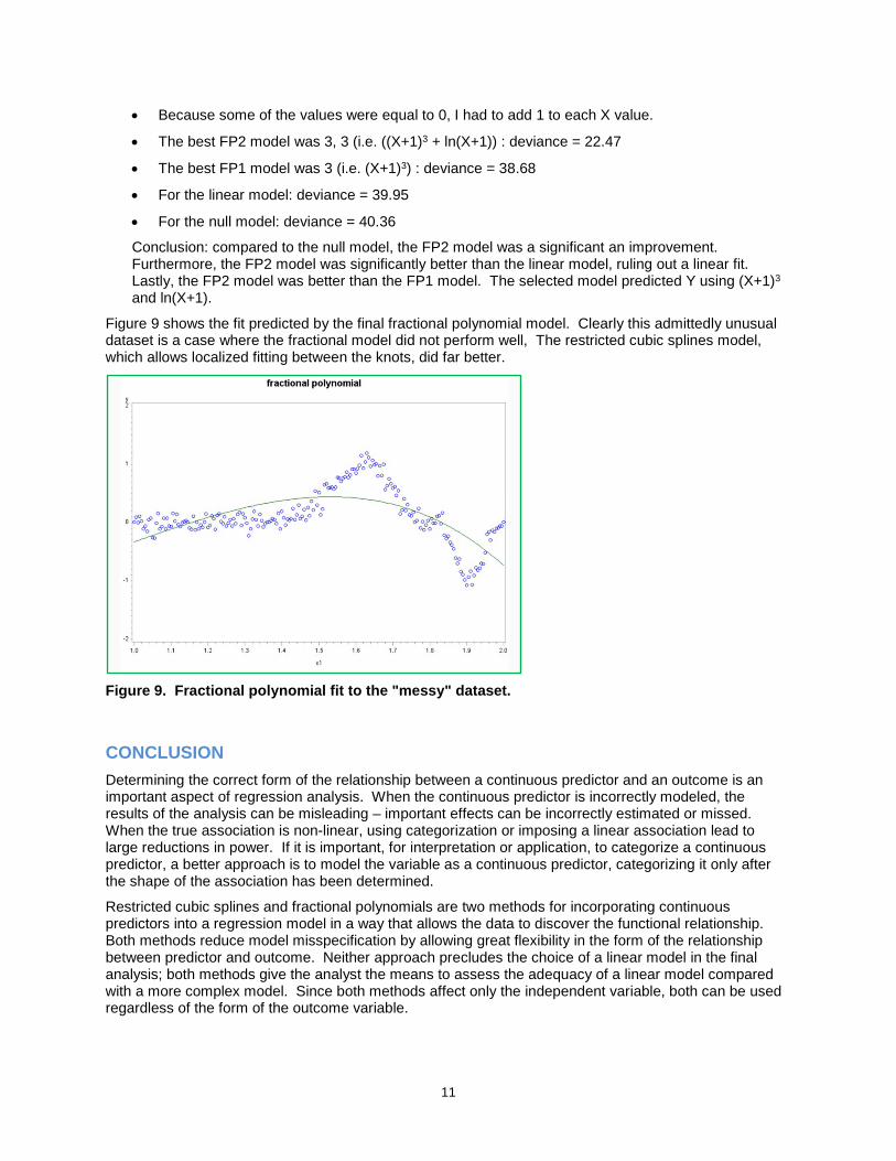
Figure 9 shows the fit predicted by the final fractional polynomial model. Clearly this admittedly unusual dataset is a case where the fractional model did not perform well, The restricted cubic splines model, which allows localized fitting between the knots, did far better.

Figure 9. Fractional polynomial fit to the "messy" dataset.

CONCLUSION Determining the correct form of the relationship between a continuous predictor and an outcome is an important aspect of regression analysis. When the continuous predictor is incorrectly modeled, the results of the analysis can be misleading – important effects can be incorrectly estimated or missed. When the true association is non-linear, using categorization or imposing a linear association lead to large reductions in power. If it is important, for interpretation or application, to categorize a continuous predictor, a better approach is to model the variable as a continuous predictor, categorizing it only after the shape of the association has been determined.

Restricted cubic splines and fractional polynomials are two methods for incorporating continuous predictors into a regression model in a way that allows the data to discover the functional relationship. Both methods reduce model misspecification by allowing great flexibility in the form of the relationship between predictor and outcome. Neither approach precludes the choice of a linear model in the final analysis; both methods give the analyst the means to assess the adequacy of a linear model compared with a more complex model. Since both methods affect only the independent variable, both can be used regardless of the form of the outcome variable.

12

While simulation studies based on single continuous predictors suggest that a fractional polynomial model is likely to provide a better fit to the data than a restricted cubic spline model, when the data contain more than one continuous predictor, a restricted cubic spline approach remains simple to implement, while implementing the fractional polynomial model may be tedious.

REFERENCES Ambler G, Royston P. Fractional polynomial model selection procedures: Investigation of type one error rate. J Stat Comput Simul. 2001;69:89–108.

Austin PC, Brunner LJ. Inflation of type type I error rate when a continuous confounding variable is categorized in logistic regression analyses. Statist Med. 2004; 23: 1159-1178.

Austin PC, Park-Wyllie LY, Juurlink DN. Using fractional polynomials to model the effect of cumulative duration of exposure on outcomes: applications to cohort and nested case-control designs. Pharmacoepidemiol Drug Saf. 2014; 23: 819-829.

Kahan BC, Rushton H, Morris TP, Daniel RM.. A comparison of methods to adjust for continuous covariates in the analysis of randomised trials. BMC Medical Research Methodology 2016; 16: 42.

Harrell Jr., F.E. (2001) Regression Modeling Strategies: with applications to linear models, logistic regression, and survival analysis. New York, NY: Springer-Verlag

Royston P, Altman DG. Regression using fractional polynomials of continuous covariates: Parsimonious parametric modelling (with discussion). Applied Statistics. 1994; 43: 429-467.

Royston P, Altman DG, Sauerbrei W. Dichotomizing continuous predictors in multiple regression: a bad idea. Statist Med. 2006; 25: 127-141.

Royston P, Sauerbrei W. (2008) Multivariable Model-Building. A pragmatic approach to regression analysis based on fractional polynomials for modelling continuous variables. Chichester, UK: Wiley.

Steyerberg EW. 2009. Clinical Prediction Models: A practical approach to development, validation and updating. New York, NY: Springer Publishing Company.

Stone, C. J. Comment: Generalized additive models. Statist Sci. 1986; 1(3), 312-314.

ACKNOWLEDGMENTS Thank you to Jiming Fang and Tetyana Kendzerska for leading the way.

CONTACT INFORMATION Your comments and questions are valued and encouraged. Contact the author at:

Ruth Croxford Institute for Clinical Evaluative Sciences, Toronto, Ontario, Canada ruth.croxford@ices.on.ca www.ices.on.ca