continuous time disaggregation in hierarchical production

University of South FloridaScholar Commons

Graduate Theses and Dissertations Graduate School

2006

Continuous time disaggregation in hierarchicalproduction planningRami Salhab Al-TamimiUniversity of South Florida

Follow this and additional works at: http://scholarcommons.usf.edu/etd

Part of the American Studies Commons

This Thesis is brought to you for free and open access by the Graduate School at Scholar Commons. It has been accepted for inclusion in GraduateTheses and Dissertations by an authorized administrator of Scholar Commons. For more information, please contact [email protected].

Scholar Commons CitationAl-Tamimi, Rami Salhab, "Continuous time disaggregation in hierarchical production planning" (2006). Graduate Theses andDissertations.http://scholarcommons.usf.edu/etd/2436

http://scholarcommons.usf.edu/?utm_source=scholarcommons.usf.edu%2Fetd%2F2436&utm_medium=PDF&utm_campaign=PDFCoverPages

http://scholarcommons.usf.edu/?utm_source=scholarcommons.usf.edu%2Fetd%2F2436&utm_medium=PDF&utm_campaign=PDFCoverPages

http://scholarcommons.usf.edu?utm_source=scholarcommons.usf.edu%2Fetd%2F2436&utm_medium=PDF&utm_campaign=PDFCoverPages

http://scholarcommons.usf.edu/etd?utm_source=scholarcommons.usf.edu%2Fetd%2F2436&utm_medium=PDF&utm_campaign=PDFCoverPages

http://scholarcommons.usf.edu/grad?utm_source=scholarcommons.usf.edu%2Fetd%2F2436&utm_medium=PDF&utm_campaign=PDFCoverPages

http://scholarcommons.usf.edu/etd?utm_source=scholarcommons.usf.edu%2Fetd%2F2436&utm_medium=PDF&utm_campaign=PDFCoverPages

http://network.bepress.com/hgg/discipline/439?utm_source=scholarcommons.usf.edu%2Fetd%2F2436&utm_medium=PDF&utm_campaign=PDFCoverPages

mailto:[email protected]

Continuous Time Disaggregation in Hierarchical Production Planning

by

Rami Salhab Al-Tamimi

A thesis submitted in partial fulfillment of the requirements for the degree of

Master of Science in Industrial Engineering Department of Industrial and Management Systems Engineering

College of Engineering University of South Florida

Major Professor: Ali Yalcin, Ph.D. Susana Lai-Yuen, Ph.D. Michael Weng, Ph.D.

Date of Approval: November 1, 2006

Keywords: production schedule, family level, minimize setup cost, production cycle, stochastic demand, out-of-stock Percentage

© Copyright 2006, Rami Salhab Al-Tamimi

Dedication

To my family

Acknowledgements

I would like to thank, my advisor, Dr. Ali Yalcin for his continual guidance and

support throughout this thesis. I also would like to thank my committee members Dr.

Susana Lai-Yuen and Dr. Michael Weng for their kind reviews and support. Finally, I

would like to thank my family, especially my fiancée, for supporting me in my

educational pursuits and my friends for their encouragement.

i

Table of Contents

List of Tables................................................................................................................. iii

List of Figures ................................................................................................................iv

Abstract ...........................................................................................................................v

Chapter 1. Introduction....................................................................................................1 1.1 Hierarchical Production Planning .............................................................1 1.2 Aggregate Planning and Disaggregation ...................................................2 1.3 Continuous Time Disaggregation..............................................................3 1.4 Motivation................................................................................................4 1.5 Research Objective...................................................................................4 1.6 Thesis Organization..................................................................................5

Chapter 2. Literature Review ...........................................................................................6 2.1 Discrete Time Disaggregation with Deterministic Demands .....................7 2.2 Discrete Time Disaggregation with Stochastic Demands ........................11 2.3 Continuous Time Disaggregation............................................................14

Chapter 3. Continuous Time Disaggregation and Backorders.........................................16 3.1 The Deterministic Continuous Time Disaggregation...............................16 3.2 Deterministic Continuous Time Disaggregation Allowing Backorder .....19 3.3 Experimental Results..............................................................................30

3.3.1 Comparison of Algorithms A1B and RKM ..................................32 3.3.2 Comparison of Algorithms A1 and A1B (Compression Effect)....36

Chapter 4. Convergence Conditions and Computational Issues ......................................39 4.1 Introduction............................................................................................39 4.2 General Convergence Expression ...........................................................42 4.3 Convergence Example and Discussion....................................................46 4.4 Comparison of Algorithms A1 and A1B Convergence Expressions ........49 4.5 A Modification to Algorithm A1B and Comparison to RKM..................50 4.6 Computational Experience with Algorithm A1B.....................................52

Chapter 5. Continuous Time Disaggregation and Demand Uncertainty ..........................55 5.1 Algorithm A1B in the Presence of Demand Uncertainty .........................55 5.2 Incorporating a Service Level Parameter in the Problem Formulation.....58

ii

Chapter 6. Conclusions and Future Work.......................................................................63 6.1 Conclusions............................................................................................63 6.2 Future Work ...........................................................................................65

References.....................................................................................................................66

iii

List of Tables

Table 3.1 Example Data.................................................................................................25

Table 3.2 Paired Comparisons of Number of Setups: n=3 ..............................................33



Table 3.5 Analysis of Differences in Number of Setups: v = 0.2 ....................................35

Table 3.6 Analysis of Differences in Number of Setups v = 0.5 .....................................36

Table 3.7 Comparisons of Number of Setups: Compression Effect Data Sets.................37


Table 4.1 Paired Comparisons of Number of Setups: n = 3 ............................................51


Table 4.3 Computational Experiment for Algorithm A1B, v = 0.5, Iavg = 2000...............53

Table 4.4 Computational Experiment for Algorithm A1, v = 0.5, Iavg = 2000 .................53

Table 5.1 Paired Comparison of Out-of-stock Percentage ..............................................56

Table 5.2 Analysis of Differences in Out-of-stock Percentage........................................57

Table 5.3 Analysis of Differences Based on Demand Variability ...................................58

Table 5.4 Comparison of Different Service Levels n = 6................................................59

iv

List of Figures

Figure 1.1 Hierarchical Production Planning Levels.........................................................1

Figure 3.1 Algorithm A1B Flowchart ............................................................................24

Figure 3.2 The Design for the Experiment .....................................................................31

Figure 3.3 Inventory Versus Time Under Algorithm A1 ................................................38

Figure 3.4 Inventory Versus Time Under Algorithm A1B..............................................38

Figure 4.1 Steps 6 and 7 from Algorithm A1B...............................................................41

Figure 4.2 Typical Relationship Between T and ][iD for Two Successive Iterations ......44

Figure 5.1 Inventory Versus Time Z1 = 0 and Z2 = 0 ......................................................61

Figure 5.2 Inventory Versus Time Z1 = -0.2 and Z2 = 0.2 ...............................................61

Figure 5.3 Inventory Versus Time Z1 = -0.5 and Z2 = 0.5 ...............................................62

v

Continuous Time Disaggregation in Hierarchal Production Planning

Rami Salhab Al-Tamimi

ABSTRACT

One of the objectives of disaggregation in hierarchical production planning is to

minimize the setup costs incurred when changing production from one family to another.

In this research, the setup costs are reduced by determining a production schedule that

minimizes the number of setups during the planning horizon. Previous solutions to the

disaggregation problem have considered discrete-time, and more recently continuous-

time formulations. This research extends the continuous time disaggregation approach by

incorporating production schedules allowing backorder. A mathematical formulation and

a solution algorithm are presented and the computational complexity and convergence

properties of the algorithm are discussed. Experimental results, using both deterministic

and stochastic demand patterns, which demonstrate the efficacies of the solution

approach are provided.

1

Chapter 1. Introduction

1.1 Hierarchical Production Planning

Production planning problems involve the scheduling of a large number of items.

Formulating such problems using mathematical programming models including all these

items is an overwhelming process. Moreover, this process includes complex decisions

that cannot be made all at once. An alternative solution to this process is the hierarchical

production planning approach (HPP) where the planning decisions are made in a

sequence. In HPP, the overall problem is divided into sub problems, where each sub

problem is related to a different hierarchal level and solved sequentially. Hax and Meal

[15] recommend three levels of HPP, as shown in Figure 1.1. The first level contains the

items which are the final products to be delivered to the customers. The second level is

the family level which is a group of items that share a common manufacturing setup. The

third level is the type level which is a group of families that have similar costs per unit of

production time, and similar seasonal demand patterns.

Figure 1.1 Hierarchical Production Planning Levels

Item 1 Item 2

Family 1

Type 1

Family 2 Family 3

Item 3 Item 4

Type Level

Family Level

Item Level

2

An example for HPP would be the planning of production in a dairy plant. In the

dairy plant, there are several dairy types like milk, ice cream, butter, cheese, eggnog and

yogurt. Each of these types includes several families that have similar costs per unit of

production time and similar seasonal demands patterns. For instance, cheese type

includes string cheese, cheddar cheese, cottage cheese, and cream cheese families. Each

cheese family contains large number of items. These items differ from each other by

characteristic such as color, packaging, labels, and accessories. As an example, cottage

cheese contains items like creamed cottage cheese, 2% and 1% cottage cheeses, dry-curd

cottage cheese, etc. These cottage cheese items differ from each others by the label, the

milk fat percentage and the drying temperature. Nevertheless, all the items within the

same family share a common manufacturing setup which is associated with a setup cost

when changing over to another family. For example, the production of the cheddar cheese

family needs specific types of mixers, cutters and dryers. Some of these machines need to

be cleaned, replaced or their parts need to be changed before starting the production of

another cheese family.

1.2 Aggregate Planning and Disaggregation

HPP consists of two steps: aggregate planning and disaggregation. Aggregate

planning is done at the types’ level with an objective of minimizing the total costs that

include production cost, inventory holding cost and labor cost according to Bitran and

Hax [5]. In the dairy plant example, each type has its own production cost, inventory

holding cost and labor cost. As an example, the milk production cost is less than the

cheese production cost while it has more inventory holding cost. All these costs are

3

included in the objective function of the aggregate planning to minimize the total cost.

The output of the aggregate planning is the number of units to be produced of each type

during each period.

Disaggregation is done at the family level. The purpose of disaggregation is to

determine a production schedule for the families with the objective of minimizing the

setup costs that are incurred during production changes from one family to another. In

addition, it also aims at maintaining consistency and feasibility between production

decisions that were made during aggregate planning and during the process of

disaggregation itself. In the dairy plant example, changing the production from the

cheddar cheese family to the cottage cheese family has a certain setup cost. The

disaggregation objective is to minimize the total setup cost within the production

schedule by minimizing the number of setups.

1.3 Continuous Time Disaggregation

Most of the previous studies of disaggregation include discrete time formulations.

These formulations determine the production schedule for the families on a single period

basis by solving the disaggregation problem at the beginning of each period.

Yalcin and Boucher [31] introduce a formulation that deals with the planning

horizon as one continuous time interval. This continuous time disaggregation

methodology looks forward to the entire planning horizon to establish common cycles of

production. During each cycle, each family is produced once. Therefore, increasing the

cycle’s length decreases the number of setups for each family. As a result, the total setup

costs are minimized. This stems from the idea in the previous section that minimizing the

4

setup costs in disaggregation can be achieved by minimizing the total number of setups

during the planning horizon.

1.4 Motivation

Due to market variation, in most practical disaggregation problems, there is a

degree of uncertainty associated with the demand for each family. The uncertainty in

demand may result in some families to go to backorder requiring the need for

disaggregation formulations that allow for backorder.

The continuous time disaggregation formulation introduced by Yalcin and

Boucher [31] shows significant improvements over the discrete time disaggregation

methods in minimizing the number of setups. However, this formulation does not allow

backorder and does not accommodate demand uncertainty. Additionally, the case of high

demand variability and low initial inventory often results in a “compression effect” [31]

where the solution tends to have more frequent setups when multiple families reach their

run-out of inventory times at approximately the same time. Allowing families to go to

backorder can resolve the compression effect problem, further reducing the number of

setups and in turn the total setup costs.

1.5 Research Objective

The goal of this thesis is to provide a continuous time disaggregation solution that

allows backorder and accommodates demand uncertainty. Within this goal, the proposed

disaggregation solution will be compared with the previous approaches through

5

experimental designs and computational properties of the solution algorithm will be

discussed.

1.6 Thesis Organization

The rest of the thesis is organized as follows: Chapter 2 reviews the previous

work in literature concerning disaggregation. Chapter 3 describes the specific problem to

be addressed, discusses the theoretical foundations and presents the continuous

disaggregation formulation allowing backorder. Chapter 4 discusses the convergence

conditions of the continuous-time disaggregation allowing backorder. Chapter 5

addresses issues associated with demand uncertainty. Finally, chapter 6 includes the

conclusion of this research and the directions for future research.

6

Chapter 2. Literature Review

Hierarchical Production Planning (HPP) was first introduced by Hax and Meal

[15] for a multiple plant, multiple product seasonal demand model. For this model, three

different hierarchical levels are introduced: items, families, and types. Items are the final

products. Families are group of items that share the same equipment and require a setup

cost when changing the production from one family to another. Types are group of

families, which have similar costs per unit of production time. The HPP is also comprised

of important planning components known as “aggregation” and “disaggregation.”

Aggregate planning is done at the type level in order to minimize the total cost, while

disaggregation is done at the family level in an attempt to minimize the setup costs.

Minimizing the setup costs is procured by determining the intermittent production

schedules during the planning horizon. For recent discussion about HPP, see Askin and

Goldberg [1] and Nahimas [23].

In this literature review, previous approaches for disaggregation are divided into

three categories. The first is discrete time disaggregation with deterministic demands.

The second is discrete time disaggregation with stochastic demands. The last is

continuous time disaggregation.

7

2.1 Discrete Time Disaggregation with Deterministic Demands

Bitran and Hax [5] propose the following family disaggregation model, that is

solved for each product type i at the beginning of each period:

Problem Pi

Minimize ,∑∈ oJj j

jj

YdS

Subject to: ∑∈

=oJj

ij XY * ,

,jjj ubYlb ≤≤ ,oJj ∈

where:

Yj: number of units of family j to be produced, Yj is the only unknown variable and it is

the output of the disaggregation model.

Sj: setup cost for family j,

dj: forecast demand for family j,

lbj and ubj: upper and lower bounds for the quantity Yj,

Xi*: total amount to be allocated among all the families belonging to type i. Xi

* has been

determined by the aggregate planning at the types level.

The lower bound, which defines the minimum production required for family j, is

given by:

[ ]jjLjjjj SSAIdddlb +−+++= + )...(,0max 1,2,1, ,

where dj+1+…+ dj+L+1 is the total forecasted demand for family j during the production

lead time L plus the review period (assumed equal one), AIj is the current available

inventory for family j, and SSj is the required safety stock for family j.

8

The upper bound is given by:

jjj AIOSub −= ,

where OSj is the overstock limit of family j.

Bitran and Hax [6] show that the first constraint of problem Pi can be relaxed

without changing the optimum solution. The constraint can be substituted by the

following:

∑∈

≤oJj

ij XY *

Following this formulation, an algorithm is introduced. This algorithm is a

Regular Knapsack Method (RKM), because the optimal value of at least one variable is

determined in each iteration. The algorithm determines the production quantities of the

families in the following period, so only those families that run-out of inventory in the

current period are considered for production. Three cases according to the upper and

lower bounds are considered. The first case is when the summation of the upper bound is

less than Xi*. In this case, all the families are produced to their upper bound limit, and

producing families that are not considered for production at this period fills the remaining

capacity. The second case is when the summation of the lower bounds is more than Xi*.

In this case backorders occur. The backorders are distributed among all the families that

are considered for production using the following formula:

o

Jjj

jJj

ji

jj Jjlb

lblbXlbY

o

o

∈−

=∑

∑

∈

∈+ ,

)( *

The last case is when Xi* lies between the lower and the upper bounds, then Algorithm

RKM is run to determine the production quantities.

9

Bitran et al. [7, 8] present a hierarchical approach to model a planning and

scheduling production problem in single stage and in two-stage manufacturing

environments. They propose some modification to the original HPP system and introduce

a mixed integer programming formulation to solve the problem. Furthermore, they

consider the infeasibility that can be introduced in the aggregate problem by the

disaggregation procedure used. Infeasibility occurs when the solution of the

disaggregation is not feasible at the aggregation level. Example of infeasibility is a

solution of one period that results in the need of more production than that allocated by

the aggregate problem to satisfy the demands of the next periods. A Look Ahead

Feasibility Rule (LAFR) is introduced. This rule looks ahead one period to prevent the

infeasibility when applying the disaggregation procedure at this period.

Saad [29] presents some modifications to Hax and Meal [15] approach to include

multi-plant multi-marketing area systems. In his approach, product types are assigned to

the plants and within each plant products are grouped in families. He includes marketing

and logistics decisions in the aggregate planning formulation to find the production

quantity for each plant. Then, the disaggregation is done at the plant level using a mixed

integer linear programming formulation.

Graves [14] presents a mixed integer programming model to solve both the

aggregate planning at the product type level and the family disaggregation. He proposes a

Lagrangean relaxation to solve the problem where the two planning levels are linked with

an inventory consistency relationship. In case of high setup costs, Graves’s test results

show a more effective solution over Bitran et al. [6]. However, this should be balanced

against the computational requirements and the complexity of his algorithm.

10

Ozdamar et al. [26] extend Bitran et al. [6] to resolve backorders that occur in the

RKM family disaggregation procedure. These backorders are the result of infeasibility

when the production quantities assigned in the aggregate planning are infeasible at the

disaggregation level. They propose a heuristic modification that eliminates this condition

and reduces the total setup costs.

Axsater [4] and Erschler [12] present conditions of consistency of the

disaggregation procedure. Given a feasible aggregate plan, the disaggregation procedure

is consistent if it satisfies the demands in the first period, and it retains the feasibility of

the aggregate plan for the rest of the planning horizon. A modified LAFR that looks

ahead over the entire horizon is then discussed.

Qui and Burch [27] and Qui [28] demonstrate a solution model to a real world

production planning and scheduling in a fiber plant using a combination of hierarchical

production planning and an expert system. At the aggregate level, the monthly lot size,

machine assignment and the ending inventory level for each individual product are

determined using the given forecast demand, machine capacities, and the total inventory

target. At the disaggregation level, with the objective of minimizing the total setup costs,

the model uses the outputs of the aggregate model to determine the sequence in which the

products are produced on their assigned machine. The disaggregation model is

formulated as a mixed integer linear program.

Discrete disaggregation approaches with deterministic demand have been

implemented widely in modern manufacturing systems. Dempster et al. [11] provide an

analytical review for disaggregation approaches using detailed production planning, job

shop scheduling, distribution system design, and vehicle routing scheduling applications.

11

Tsubone and Sugawara [30] present an HPP that includes feedback between the

hierarchical levels based on human judgments for motor industry applications. Nguyen

and Dupont [25] consider an HPP approach in steel manufacturing firm which works on

demands according to each customer’s requirements. Akturk and Wilson [2] apply an

HPP approach in cellular manufacturing system by introducing several enhancements to

Hax and Meal [15] HPP approach. Neureuther et al. [24] introduce a non-linear

disaggregation model for a strictly make-to-order steal fabrication plant.

2.2 Discrete Time Disaggregation with Stochastic Demands

Bitran et al. [9] consider a manufacturing of style goods application. Style goods

have very short selling seasons and the demands are changing over time. This

characteristic requires a continuous revision of the forecasted demands over the planning

horizon. They formulate the problem as a mixed integer stochastic program. As this

formulation is hard to solve, two-stage hierarchical approach is proposed to solve this

problem. Furthermore, the products are grouped into families where the means of the

demands are assumed to be known. The first stage of the approach is the aggregate

problem which is formulated as a deterministic mixed integer program that provides a

lower bound on the optimal solution. The solution to this problem determines the set of

product families to be produced in each period. The second stage is a disaggregation

stage where item lot sizes are determined for families scheduled in each period. Matsuo

[20] extends this approach by a stochastic sequencing formulation that simultaneously

determines product sequence. His sequencing rule based on the ratio of the inventory

12

holding cost plus the expected value of additional information per unit time to the

expected resource consumption of a family.

Ari and Axsater [3] consider HPP disaggregation in the case of stochastic

demands where the item demands are assumed to be independent stochastic variables

with known distributions. Moreover, they are known for the current period, but are still

unknown for the rest of the planning horizon. A dynamic programming algorithm is

introduced with an objective of maximizing the probability of feasibility of the aggregate

plan. The optimal solution is proved to be the same as minimizing the differences

between the inventory levels at the end of each period which is referred to as the simple

disaggregation rule. This rule is applicable for many common demand distributions.

However, according to the authors, because of the set up costs it is, in general, not

possible to apply the simple disaggregation rule making the inventories as equal as

possible.

Lasserre and Merce [19] consider a robust aggregate plan that provides a

disaggregation policy that can handle the variation in the demands. The items demands

are known for the current period, while for the rest of the planning horizon they vary

within given bounds. According to the authors, the aggregate plan is said to be robust if

and only if for any potential demand there exists a feasible disaggregation policy.

Necessary and sufficient conditions for robustness are presented. These conditions are

converted to constraints in aggregate planning, which take into account the uncertainty of

the demands. Gfrerer and Zapfel [13] propose a generalization for the robustness concept

by introducing two sets of sufficient conditions of robustness using the concept of static

13

and dynamic demand schemes. In addition, simplifications to these conditions are

introduced for implementation purposes.

Another stochastic linear programming approach is introduced by Kira [18]. This

approach is a modification of Bitran’s and Hax’s [5] formulation that elaborate penalties

for infeasibility. Two penalties are introduced: surplus and shortage, which give an upper

and a lower bound for the production for each family. Their formulation shows some

improvement over Bitran and Hax [5] formulation with the largest average improvement

occurring with the highest expected demand and the smallest with the lowest expected

demand.

Yan [32-36] explores the hierarchical stochastic production planning problem of

flexible automated work shops in an agile manufacturing environment. Yan [32] and [35]

present a nonlinear model of stochastic production with delay interaction. They have

developed a software package named SPID with an algorithm based on their model. In

Yan [33], a stochastic nonlinear programming model whose constraints are linear and a

piecewise linear is formulated. This model is transformed into a deterministic nonlinear

programming model then into a linear programming one to simplify the solution. Two

algorithms are proposed to solve this model. The first algorithm is Karmarkar algorithm

[17]. The second is an interaction/prediction algorithm. Yan proposes that this approach

is capable of solving more complicated manufacturing systems with multi-period multi-

product problems. In Yan [34], the approach is implemented to a multi-period multi-

product problem. A software package named SIPA has been developed based on the

stochastic interaction/prediction algorithm.

14

Incorporating stochastic demand patterns has gained attention in modern

manufacturing systems. Dempster et al. [11] present a multistage stochastic model for a

job shop design problem. Ciarallo et al. [10] discuss the characteristics of the effect of

random capacity and demand uncertainty on periodic review, production planning

decisions. Kasilingam [16] proposes a non-linear programming formulation for solving

the capacity allocation problem considering stochastic demands in air cargo yield

management. Mulvey and Ruszczynski [22] consider a decomposition method for multi-

stage stochastic scheduling and transportation problem. Yokoyama and Lewis [38]

introduce two heuristic algorithms for a multi-product multi-machine production system

where the demand in each period is a mutually independent random variable whose

probability distribution is known. Yin et al. [37] present a stochastic approach to

incorporate demand uncertainties in paper industry.

2.3 Continuous Time Disaggregation

Yalcin and Boucher [31] introduce a continuous time solution method to the

disaggregation problem. This continuous time solution looks forward to the entire

planning horizon to establish common cycles of production. During each cycle each

family is produced once.

This solution is formulated as a set of linear equations that can be solved

simultaneously. The formulation is solved for T , ][it , i = 1, …, n, and given by:

TMax ,

s.t. )1...(2,1,0][][ ][][][][]1[0],[ −=≥+−−+ + niDTtPttI iiiiii , (1-1)

15

niDTtPtTI iiiii =≥+−−+ ,0][][ ][][][][0],[ , (1-2) nirt ii ...2,1,][][ =≤ , (1-3) where ][iP is the average production rate over the period t[i] to t[i+1]; ][iD is the average

demand rate over the period 0 to ][ ][ Tt i + ; ][it and ]1[ +it is the time to start and stop

producing family i; n is the number of families considered for disaggregation; and ][ir is

the run-out of inventory time for family i that can be found by solving the following

equality.

0][

0],[0],[ =− ∫

=

dtDIir

ttii

The objective of the above formulation is to maximize the length of the cycle time

T. Since each family is produced once in each cycle, maximizing the cycle time decreases

the number of setups during the planning horizon, as a result the setup costs are

minimized. The constraints (1-1) and (1-2) of the formulation ensure that supply meets

demand over the cycle. The last constraint (1-3) ensures that the production of family i

begins before it runs out of inventory.

Several properties for the optimal solution are considered. ][iP and ][iD depend on

the value of T. Therefore, an initial value for T has to be estimated before solving the

formulation. The proposed estimation is the time when the last family runs out. An

iterative algorithm is proposed to solve this formulation. The experimental results of

Yalcin and Boucher [31] algorithm demonstrate a better performance and a significant

difference in the number of the setups of the proposed algorithm over the Algorithm

RKM.

16

Chapter 3. Continuous Time Disaggregation and Backorders

This chapter discusses the fundamentals of the continuous time disaggregation

formulation. Then, it presents the continuous disaggregation formulation allowing

backorder along with experimental results. This chapter is divided into 3 sections. Section

3.1 discusses in detail the continuous time disaggregation formulation and algorithm

introduced by Yalcin and Boucher [31] which forms the basis for the work in this thesis.

Section 3.2 introduces a modified formulation that allows families to go to backorder,

some interesting properties of the formulation, and an iterative algorithm to solve the

formulated problem. In section 3.3, experimental results comparing the performance of

the formulation allowing backorders are illustrated.

3.1 The Deterministic Continuous Time Disaggregation

Continuous time disaggregation is formulated as a set of linear equations as

follows:

TMax , (3-1a)

s.t. )1...(2,1,0][][ ][][][][]1[0],[ −=≥+−−+ + niDTtPttI iiiiii , (3-1b) niDTtPtTI iiiii =≥+−−+ ,0][][ ][][][][0],[ , (3-1c) nirt ii ...2,1,][][ =≤ , (3-1d)

17

where ][iP is the average production rate over the period t[i] to t[i+1] ; ][iD is the average

demand rate over the period 0 to ][ ][ Tt i + ; ][it is the time to start producing family i; ]1[ +it

is the time to stop producing family i; n is the number of families considered for

disaggregation; and ][ir is the run-out of inventory time that can be found by solving the

following equality:

0][

0],[0],[ =− ∫

=

dtDIir

ttii (3-1e)

The objective function of this formulation is maximizing the cycle time.

Maximizing the cycle time decreases the number of setups during the planning horizon,

and as a result the setup costs are minimized.

Constraints (3-1a) and (3-1b) ensure that inventory and production meets the

demand over the cycle T . For each family the summation of its current inventory and its

production during the cycle should be equal to or greater than the demand in that cycle.

The last constraint (3-1d) ensures that family production will start before it runs

out of inventory. Although the previous constraints will guarantee that by the end of the

cycle all the demands will be satisfied, they do not prevent the families from going to

backorder before the start of their production during the cycle time. This constraint will

ensure that families will not go to backorder by forcing the production to start before the

run-out of inventory time of each family.

The deterministic continuous time formulation is iterative. To solve for the cycle

time, initial values for the average demands should be calculated. However; the average

demand for each family depends on the value of the cycle time which requires an initial

value for T. As some variables have to be determined by a decision variable, an

18

algorithmic approach is used. The following algorithm is called A1, and is used to solve

the deterministic continuous time disaggregation formulation:

Algorithm A1

Step 1: Initialize a counter, j=0, and a convergence tolerance level, ∆ .

Step 2: Order families in ascending order of their run-out times.

Step 3: Place all families in the set F, which is an ordered set of families currently

being considered for disaggregation. For n families in F, let k = n.

Step 4: Initialize T0 = r[n]. Initialize ][iP and ][iD as follows:

0

[ ] [ ],0 0

1 T

i i tP P dtT

= ∫

0

[ ] [ ],0 0

1 T

i i tD D dtT

= ∫ .

Step 5: Increment j. Solve the following equation.

)1...(2,1,0][][ ][][][][]1[0],[ −==+−−+ + niDTtPttI iiiiii Step 6: Using solution values from Step 5, compute, for all families in F:

dtPtt

Pi

i

t

tti

iii ∫

+

−=

+

]1[

[ ]],[

][]1[][

1

[ ]

[ ] [ ],[ ] 0

1 it T

i i ti

D D dtt T

β

β

+

=+ ∫

Increment j. Step 7: Solve the following equation set:

[ ],0 [ 1] [ ] [ ] [ ] [ ]

[ ],0 [ ] [ 1] [ 1] [ 1] [ 1]

[ ] [ ] 0 , 1, 2, 3 ...( 2)

[ ] [ ] 0i k i i i i

k k k k k k

I t t P t T D i k

I r t P t T D−

− − − −

+ − − + = = −

+ − − + =

19

If ∆<− −1jj TT , go to Step 8. Else, go to Step 6.

Step 8: Evaluate the condition irt ii ∀≤ ][][ . If true, stop. This is a valid solution. If

false, go to Step 9.

Step 9: Set k = the largest number i in F for which ][][ ii rt > is true. Delete from F all

families where ki > . Go to Step 1.

3.2 Deterministic Continuous Time Disaggregation Allowing Backorder

The last constraint in the deterministic continuous time formulation prevents

families from going to backorder. If this constraint is eliminated, families are allowed to

start their production before or after their run-out of inventory time during a given cycle

which allows the families to go to backorder. The formulation is as follows:

TMax , (3-2a)

s.t.

)1...(2,1,0][][ ][][][][]1[0],[ −=≥+−−+ + niDTtPttI iiiiii , (3-2b)

niDTtPtTI iiiii =≥+−−+ ,0][][ ][][][][0],[ , (3-2c)

Although the only difference between the two formulations is the last constraint,

deleting this constraint changes the properties of the optimal solution. Several properties

of the deterministic continuous time formulation allowing backorder are described below.

Property 1:

In any optimal solution, equations (3-2b) and (3-2c) will be equalities. Although

any family can go to backorder during the production cycle, at the end of the cycle all the

demands should be satisfied.

20

Proof:

Let P be the average aggregate production rate over the period 0-T, i.e.,

})(])[({1][][][][

1

1]1[ nnii

n

ii PtTPtt

TP −+−= ∑

−

=+ . Since ][iP and ][iD are in the same aggregate

units, equations (3-2b) and (3-2c) can be combined as follows:

∑∑∑===

+≥+n

iii

n

ii

n

ii DTDtPTI

1][][

1][

10],[ , (3-3)

If there existed a solution to equations (3-2b) and (3-2c) in which the inequality of

equation (3-3) holds, then the solution could be improved by increasing T until equation

(3-3) becomes an equality. Therefore, any optimal solution is a solution in which

constraints (3-2b) and (3-2c) are equalities.

The significance of this property is that an optimal solution can be obtained from

a solution of n simultaneous equations of the form:

)1...(2,1,0][][ ][][][][]1[0],[ −==+−−+ + niDTtPttI iiiiii (3-4a) niDTtPtTI iiiii ==+−−+ ,0][][ ][][][][0],[ (3-4b) and t[1] = 0. Since t[1] = 0, for n products, there will be n simultaneous equations with n

unknowns (t[i], i = 2,3,…n, and T).

Note that, in equation (3-3), the left hand side includes the supply of production

time allocated to the cycle, T; i.e., PT . The right hand side is the demand during the

cycle, T. Since, in any optimal solution, equation (3-3) must be an equality, the period T

will be determined by equilibrium of the supply and the demand. In effect, more demand

can be serviced by increasing the production cycle time, T on the right hand side of

equation (3-3).

21

Property 2:

If, in an optimal solution to equations (3-4a) and (3-4b), [ ] [ ]nn rt < , then the cycle

time of the first (n-1) families will be increased by solving equation (3-4a) alone and

letting [ ] [ ]nn rt = . However; if, in an optimal solution to equations (3-4a) and (3-4b),

[ ] [ ]nn rt > , then the cycle time of the first (n-1) families will be decreased by solving

equation (3-4a) alone.

Proof:

In Property 1, we noted that more demand can be serviced by increasing the

production cycle time, T. When equations (3-4a) and (3-4b) are solved, the total

production time allocated to the first (n-1) families is:

]1[)]1[][(

2

1 ][)

][]1[(

1

1 0],[ −−−+−

=−

++∑

−

=∑ nPnt

nt

n

i iP

it

it

n

i iI (3-5)

If equation (3-4b) is dropped and [ ] [ ]nn rt = is imposed, the total production time

allocated to the first (n-1) families is:

]1[)]1[][(2

1][)][]1[(

1

1 0],[ −−−+−

=−++∑

−

=∑ nPntnr

n

iiPitit

n

i iI (3-6)

Subtracting (3-5) from (3-6) yields: ]1[][]1[][ −−− nP

ntnP

nr (3-7)

When [ ] [ ]nn rt < is true, more production time is allocated to the first (n-1) products and T

will be greater under (3-6) than (3-5). On the other hand, when [ ] [ ]nn rt > , T will be greater

under (3-5) than (3-6).

22

Property 2 suggests that maximizing the cycle time T first require solving

equations (3-4a) and (3-4b) for all families n. Secondly, the value of [ ]nt is compared

to [ ]nr . If [ ] [ ]nn rt > then this is the solution that maximizes T, and the algorithm is run

again at time T. If [ ] [ ]nn rt < then letting [ ] [ ]nn rt = and solving equation (3-4a) alone will

result in larger cycle time T, and the algorithm will be run again at time [ ]nr .

The deterministic continuous time formulation allowing backorder is also iterative

since an initial value of T should be assigned to calculate the initial values of the average

demands. The following algorithm (Algorithm A1B) is proposed as an algorithmic

approach for the solution of this formulation.

Algorithm A1B

Step 1: Initialize a counter, j = 0, and a convergence tolerance level, ∆ .

j is the iteration index. ∆ is the level of convergence. If the difference between

two successive cycle time, T is ∆ the algorithm considers T as an optimal

solution.

Step 2: Order families in ascending order of their run-out times r[i], i = 1, …, n.

Where n is the number of families, and r[i] is the solution to:

0][

0],[0],[ =− ∫

=

dtDIir

ttii

Step 3: Place all families in the set F, which is an ordered set of families currently being

considered for disaggregation.

Step 4: Initialize T0 = r[n]. Initialize ][iP and ][iD as follows:

23

0

[ ] [ ],0 0

1 T

i i tP P dtT

= ∫

∫= 0

0 ],[0

][1 T

tii dtDT

D

Step 5: Increment j. Solve equation set (3-4).

Step 6: Using solution values, compute, for all families in F:

dtPtt

Pi

i

t

tti

iii ∫

+

−=

+

]1[

[ ]],[

][]1[][

1

∫+

+= ji Tt

tiji

i dtDTt

D ][

0 ],[][

][1

Step 7: Increment j. Solve equation set (3-4). If ∆≥− −1jj TT , go to step 6.

Step 8: If [ ] [ ]nn rt > this is a valid solution (end), else go to step 9.

Step 9: Set j = 0. Initialize T0 = r[n]. Initialize ][iP and ][iD , i = 1, …, n, as follows:

0

[ ] [ ],0 0

1 T

i i tP P dtT

= ∫

∫= 0

0 ],[0

][1 T

tii dtDT

D

Step 10: Increment j. Solve equation set (3-4a). (Note (3-4b) is not included)


dtPtt

Pi

i

t

tti

iii ∫

+

−=

+

]1[

[ ]],[

][]1[][

1

∫+

+= ji Tt

tiji

i dtDTt

D ][

0 ],[][

][1

Step 12: Increment j. Solve equation set 3-4a. If ∆≥− −1jj TT , go to step 11, else end

this is a valid solution.

24

If the valid solution is the result of solving equation set (3-4) then the algorithm is

run again at time T when family n ends its production. However; if the valid solution is

the result of only solving 3-4a then the algorithm is run again at time [ ]nr when family n-1

ends its production. Algorithm A1B is demonstrated using a flowchart in Figure 3.1

followed by a numerical example.

Start

Order families according to their

run out times

Compute P(i)and D (i)

|Tj – Tj-1| ≥ ∆

j = j + 1Solve equation set (3-4)

End

No

Yes

j = 0T0 = r(n)


t(n) < r(n)

Yes

Compute P(i)and D(i)

|Tj – Tj-1| ≥ ∆

j = j + 1Solve equation (3-4a) Yes

j = 0T0 = r(n)


No

No

j = j + 1Solve Equation Set (3-4)

j = j + 1Solve Equation (3-4a)

Figure 3.1 Algorithm A1B Flowchart

25

Example Problem: Consider the data of Table (3.1) showing the initial inventory,

I0 and product demand, Dt for three products over six periods. Pt is the aggregate

production rate.

Table 3.1 Example Data

Period Dt Family A Dt Family B Dt Family C Pt Production 1 1054.2 838.3 807.9 3000.02 1170.0 843.2 1188.8 3000.03 1158.9 982.1 1154.6 3000.04 1026.0 1170.5 1029.8 3000.05 1129.6 1052.9 1086.0 3000.06 885.1 863.5 1108.4 3000.0I0 2000.0 1000.0 0.0

Step 1: Initialize a counter, j = 0, and a convergence tolerance level, ∆ = 0.01.

Step 2: The number of families n = 3. Compute each family run-out time.

rA = 1.808, rB = 1.192, and rC = 0.

Order them in ascending order.

r[1] = rC = 0; r[2 ]= rB = 1.192; r[3] = rA = 1.808.

Step 3: Place all families in the set F = {C, B, A}.

Step 4: Initialize T as the last family in set F run-out time; T0 = r[3] = 1.808.

Initialize ][iP and ][iD , i = 1, …, n ,as follows:

[ ] 3000808.1

)3000)(808.0(30001 =+=P , which is the same for all i.

0.1106808.1

)0.1170)(088.0(2.1054

5.840808.1

)2.843)(088.0(3.838

2.978808.1

)8.1188)(808.0(9.807

]3[

]2[

]1[

=+=

=+=

=+=

D

D

D

26

Step 5: Increment j; j = 1.

Solve for 1T , ]1[t , ]2[t , and ]3[t .

0][][ ]1[]1[]1[]1[]2[0],1[ =+−−+ DTtPttI

0][][ ]2[]2[]2[]2[]3[0],2[ =+−−+ DTtPttI

0][][ ]3[]3[]3[]3[0],3[ =+−−+ DTtPtTI

0]2.978][[]3000][[0 1]1[]1[]2[ =+−−+ Tttt

0]5.840][[]3000][[1000 1]2[]2[]3[ =+−−+ Tttt

0]0.1106][[]3000][[2000 1]3[]3[1 =+−−+ TttT

Solution: 1T = 3.47, ]1[t = 0, ]2[t = 1.13, and ]3[t = 2.09.

Step 6: Using the solution from step 5, compute ][iP and ][iD for all i

[ ] 3000=iP .

3.108556.5

)1.885)(56.0(6.11290.10269.11580.11702.1054

9.97060.4

)8.1052)(60.0(5.11701.9822.8433.838

6.047147.3

)8.1029)(47.0(6.11548.11889.807

]3[

]2[

]1[

=+++++=

=++++=

=+++=

D

D

D



0]6.1047][[]3000][[0 2]1[]1[]2[ =+−−+ Tttt

0]9.970][[]3000][[1000 2]2[]2[]3[ =+−−+ Tttt

27

0]3.1085][[]3000][[2000 2]3[]3[2 =+−−+ TttT


∆≥− 12 TT , go to step 6.


[ ] 3000=iP .

2.110420.4

)6.1129)(20.0(0.10269.11580.11702.1054

3.92850.3

)5.1170)(50.0(1.9822.8433.838

2.103459.2

)6.1154)(59.0(8.11889.807

]3[

]2[

]1[

=++++=

=+++=

=++=

D

D

D



0]2.1034][[]3000][[0 3]1[]1[]2[ =+−−+ Tttt

0]3.928][[]3000][[1000 3]2[]2[]3[ =+−−+ Tttt

0]2.1104][[]3000][[2000 3]3[]3[3 =+−−+ TttT


∆≥− 23 TT , go to step 6.

Steps 6 and 7 are repeated till convergence occurs at 8T .

8T = 2.69, ]1[D = 1038.7, ]2[D = 936.88, ]3[D = 1104.92, ]1[t = 0, ]2[t = 0.93, and

]3[t = 1.73.

Step 8: [ ] [ ]33 rt < solving 3-4a alone will result in larger T. Go to step 9.

28

Step 9: Set j = 0. Initialize T0 = r[3] = 1.808.

Initialize ][iP and ][iD , i = 1, …, n ,as follows:

[ ] 30001 =P , which is the same for all i.

5.840

2.978

]2[

]1[

=

=

D

D


Solve for 1T , ]1[t , and ]2[t .

0][][ ]1[]1[]1[]1[]2[0],1[ =+−−+ DTtPttI

0][][ ]2[]2[]2[]2[]3[0],2[ =+−−+ DTtPtrI

0]2.978][[]3000][[0 1]1[]1[]2[ =+−−+ Tttt

0]5.840][[]3000][[1000 1]2[]2[]3[ =+−−+ Tttr

Solution: 1T = 3.07, ]1[t = 0 and ]2[t = 1.00.


[ ] 3000=iP .

2.960

07.4)8.1052)(60.0(5.11701.9822.8433.838

0.050107.3

)8.1029)(07.0(6.11548.11889.807

]2[

]1[

=++++=

=+++=

D

D



0]0.1050][[]3000][[0 1]1[]1[]2[ =+−−+ Tttt

29

0]2.960][[]3000][[1000 1]2[]2[]3[ =+−−+ Tttr

Solution: 2T = 2.74, ]1[t = 0, and ]2[t = 0.96.

∆≥− 12 TT , go to step 11.


[ ] 3000=iP .

2.941

70.3)5.1170)(70.0(1.9822.8433.838

5.040174.2

)6.1154)(74.0(8.11889.807

]2[

]1[

=+++=

=++=

D

D



0]5.1040][[]3000][[0 1]1[]1[]2[ =+−−+ Tttt

0]2.941][[]3000][[1000 1]2[]2[]3[ =+−−+ Tttr

Solution: 2T = 2.78, ]1[t = 0, and ]2[t = 0.97.

∆≥− 23 TT , go to step 11.


[ ] 3000=iP .

4.944

75.3)5.1170)(75.0(1.9822.8433.838

3.042178.2

)6.1154)(78.0(8.11889.807

]2[

]1[

=+++=

=++=

D

D

30



0]3.1042][[]3000][[0 1]1[]1[]2[ =+−−+ Tttt

0]4.944][[]3000][[1000 1]2[]2[]3[ =+−−+ Tttr

Solution: 2T = 2.78, ]1[t = 0, and ]2[t = 0.96.

∆<− −1jj TT . Convergence occurs.

*T = 4T = 2.78, ]1[t = 0, and ]2[t = 0.96.

At this point, the solution is accepted up to [ ]3r . When the time reaches [ ]3r , the

algorithm is run again to find the production periods for the next cycle.

Recalling property 2, in this example, when solving equation set (3-4), it is

found that [ ] [ ]33 rt < . As a result, solving equation 3-4a alone results in *T = 2.79 which is

larger than *T = 2.69 when solving equation set (3-4).

3.3 Experimental Results

Following the experimental design and the data sets in [31], Algorithms A1B and

RKM are compared. Figure 3.1 illustrates the experimental design. Three control

parameters are used to generate different data sets for the experiment. These parameters

are: the number of families n, the amount of the average initial inventory Iavg, and the

demand variability v.

31

Figure 3.2 The Design for the Experiment

In Algorithm A1B, the number of families n determines the number of setups

during each production cycle. For instance, if the number of families is n, the number of

setups will be either n or n-1 during each production cycle. Three levels are used in the

experimental data sets for the number of families: three, six and nine.

The level of the average initial inventory is a factor that constrains the number of

setups during the planning horizon. The average initial inventory (Iavg) determines the

run-out of inventory time for each family and affects the length of the production cycle

since at the end of the cycle time all the demands during that cycle must be satisfied. If

the initial inventory is high, the production time available for each family will be longer.

Three total initial inventory levels are used: one, two and three periods of supply.

Two levels of demand variability are used: low variability and high variability. A

uniform distribution is used to generate the demands for each family for a 12 period

planning horizon which is assumed to reoccur every 12 periods. The average demand

which is the mean of the distribution is 1000 units. The distribution limits are as follows:

nv

Iavg

9

630.5

0.2

1

2

3

32

DvDD

DvDD

×+=

×−=

max

min

For low variability v is set to 0.2, and for high variability is set to 0.5.

The production rate is defined as a function of the number of families and the

average demand. It is set as 3000, 6000 and 9000 for three, six and nine families.

3.3.1 Comparison of Algorithms A1B and RKM

Algorithm A1B is compared with Algorithm RKM since both algorithms allow

backorder. The comparison results of the number of setups are summarized in Tables 3.2,

3.3, and 3.4. The data sets are grouped in the tables according to the number of families,

and then each table is divided according to the variability and the initial inventory levels.

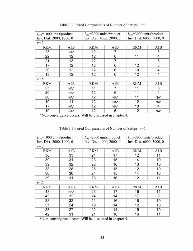
The results show that the number of setups using Algorithm A1B is less than the

number of setups using Algorithm RKM for all data sets. Note that, as the number of

families increases the difference between the numbers of setups for the two algorithms

decreases. Table 3.2, 3.3, and 3.4 show that the average number of setups using

Algorithm A1B is between 37.3-59.6% for n = 3, 18.4-33.7% for n = 6, and 16.1-31.7%

for n = 9 fewer than the average number of setups using Algorithm RKM. However, the

average initial inventory and the demand variability do not affect the difference between

the numbers of setups between the two algorithms.

33

Table 3.2 Paired Comparisons of Number of Setups: n=3

Iavg=1000 units/product Inv. Dist. 2000, 1000, 0



v=.2 RKM A1B RKM A1B RKM A1B

23 NA* 12 7 11 5 22 12 12 6 11 4 21 13 12 7 11 5 17 12 12 6 12 5 20 12 12 6 10 4 18 12 12 6 12 4


25 NA* 11 7 11 5 20 NA* 12 6 11 4 20 NA* 12 NA* 11 NA* 19 11 12 NA* 12 NA* 17 NA* 12 NA* 10 4 19 NA* 12 6 12 NA*

*Non-convergence occurs. Will be discussed in chapter 4.






36 33 24 17 12 11 39 31 23 15 14 10 39 32 23 16 13 10 38 28 25 15 12 10 36 30 24 15 14 10 39 31 23 16 12 11


48 NA* 23 17 16 11 43 32 24 14 17 9 38 32 21 16 16 10 37 24 19 14 12 10 33 27 22 14 15 10 42 31 21 16 16 11


34






59 50 38 25 29 17 54 47 35 24 25 15 56 50 35 25 22 16 58 45 35 24 23 16 60 46 31 24 19 16 58 51 43 25 24 17


57 52 35 25 25 18 58 46 31 20 27 14 62 48 33 25 20 16 51 43 30 23 22 16 57 43 32 23 23 15 66 NA* 41 27 24 17


A paired-sample t-test [21] is performed in the differences between means, dµ , for

paired trials. The test considers the hypothesis:

.0:,0:

1

0

≠=

d

d

HH

µµ

The test statistics is:

nS

dtd /0 =

Where:

)1()(

11

BAxRKMxd

dn

d

jjj

n

jj

−=

= ∑=

)(RKMx j = number of setups on trial j for Algorithm RKM

35

)1( BAx j = number of setups on trial j for Algorithm A1B

1

)1( 2

11

2

−

−=

∑∑==

m

dn

dS

n

jj

n

jj

d

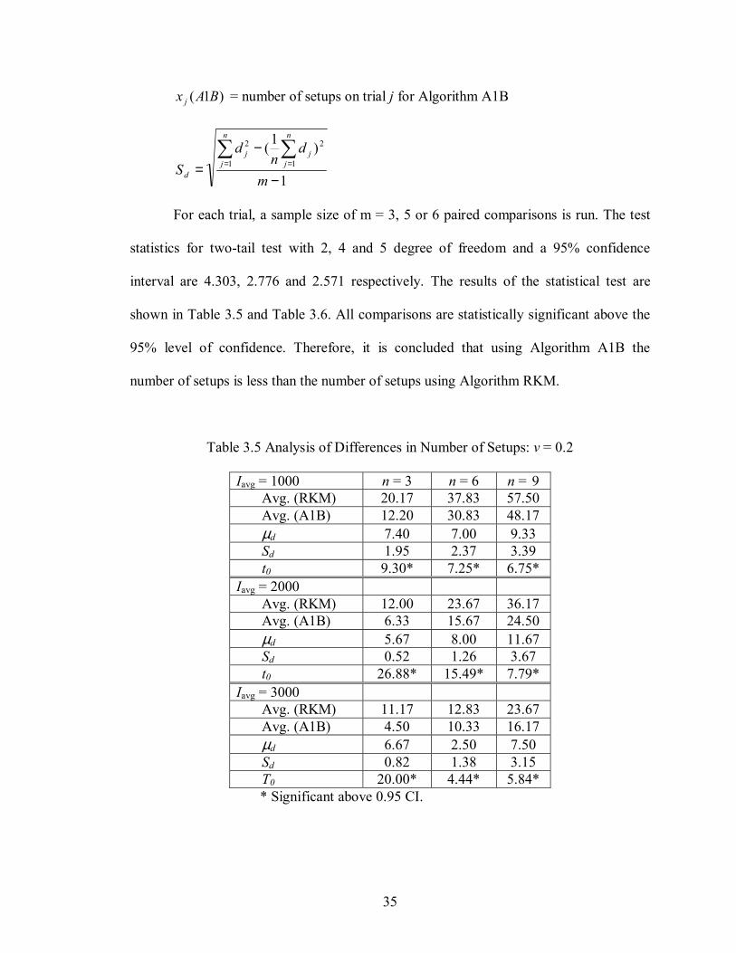
For each trial, a sample size of m = 3, 5 or 6 paired comparisons is run. The test

statistics for two-tail test with 2, 4 and 5 degree of freedom and a 95% confidence

interval are 4.303, 2.776 and 2.571 respectively. The results of the statistical test are

shown in Table 3.5 and Table 3.6. All comparisons are statistically significant above the

95% level of confidence. Therefore, it is concluded that using Algorithm A1B the

number of setups is less than the number of setups using Algorithm RKM.

Table 3.5 Analysis of Differences in Number of Setups: v = 0.2

Iavg = 1000 n = 3 n = 6 n = 9 Avg. (RKM) 20.17 37.83 57.50 Avg. (A1B) 12.20 30.83 48.17 µd 7.40 7.00 9.33 Sd 1.95 2.37 3.39 t0 9.30* 7.25* 6.75* Iavg = 2000 Avg. (RKM) 12.00 23.67 36.17 Avg. (A1B) 6.33 15.67 24.50 µd 5.67 8.00 11.67 Sd 0.52 1.26 3.67 t0 26.88* 15.49* 7.79* Iavg = 3000 Avg. (RKM) 11.17 12.83 23.67 Avg. (A1B) 4.50 10.33 16.17 µd 6.67 2.50 7.50 Sd 0.82 1.38 3.15 T0 20.00* 4.44* 5.84*

* Significant above 0.95 CI.

36

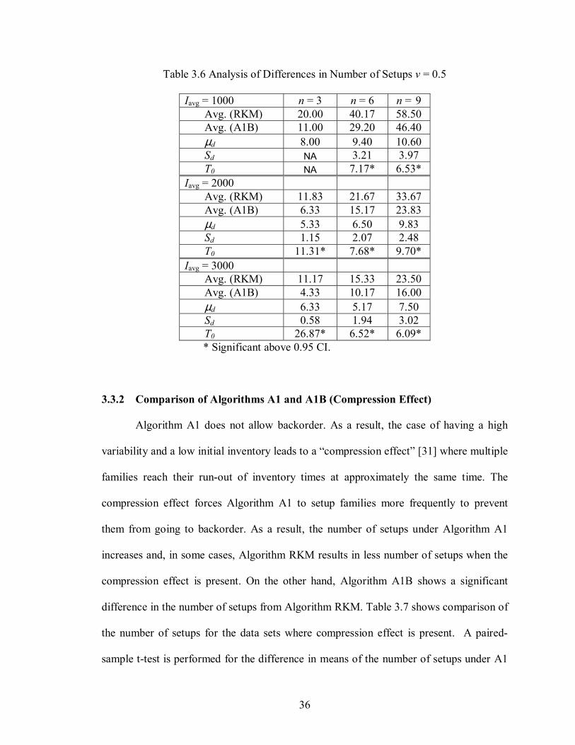
Table 3.6 Analysis of Differences in Number of Setups v = 0.5

Iavg = 1000 n = 3 n = 6 n = 9 Avg. (RKM) 20.00 40.17 58.50 Avg. (A1B) 11.00 29.20 46.40 µd 8.00 9.40 10.60 Sd NA 3.21 3.97 T0 NA 7.17* 6.53* Iavg = 2000 Avg. (RKM) 11.83 21.67 33.67 Avg. (A1B) 6.33 15.17 23.83 µd 5.33 6.50 9.83 Sd 1.15 2.07 2.48 T0 11.31* 7.68* 9.70* Iavg = 3000 Avg. (RKM) 11.17 15.33 23.50 Avg. (A1B) 4.33 10.17 16.00 µd 6.33 5.17 7.50 Sd 0.58 1.94 3.02 T0 26.87* 6.52* 6.09*


3.3.2 Comparison of Algorithms A1 and A1B (Compression Effect)

Algorithm A1 does not allow backorder. As a result, the case of having a high

variability and a low initial inventory leads to a “compression effect” [31] where multiple

families reach their run-out of inventory times at approximately the same time. The

compression effect forces Algorithm A1 to setup families more frequently to prevent

them from going to backorder. As a result, the number of setups under Algorithm A1

increases and, in some cases, Algorithm RKM results in less number of setups when the

compression effect is present. On the other hand, Algorithm A1B shows a significant

difference in the number of setups from Algorithm RKM. Table 3.7 shows comparison of

the number of setups for the data sets where compression effect is present. A paired-

sample t-test is performed for the difference in means of the number of setups under A1

37

and A1B. Table 3.8 summarizes the statistical analysis results which show significant

differences between the means above the 95% level of confidence. According to the

results, the average number of setups using Algorithm A1B is between 16.5-17% less

than the average number of setups using Algorithm A1.

Table 3.7 Comparisons of Number of Setups: Compression Effect Data Sets

Iavg=1000 units/product Inv. Dist. 2000, 1000, 0 v=.5

N = 6 n = 9 RKM A1 A1B RKM A1 A1B

39 43 32 57 66 52 36 38 32 58 53 46 29 37 24 62 61 48 30 33 27 51 49 43 42 42 31 57 49 43


Iavg = 1000 n = 6 n = 9 Avg. (A1) 35.20 55.60 Avg. (A1B) 29.20 46.40 µd 6.00 9.20 Sd 3.16 3.96 T0 4.65* 5.69*


To fully illustrate the effectiveness of Algorithm A1B in reducing compression

effect period, inventory versus time graphs are shown in Figures 3.2 and 3.3 for

Algorithms A1 and A1B for a family with initial inventory of 1200 units and n = 6. The

inventory increase in the figures represents the duration when this family is in production.

At time 2.9 and 5.9 in Figure 3.4, there are two short time production periods which

result in two setups. These two setups disappeared in Figure 3.5 by allowing the family to

38

go to backorder. It is concluded that allowing backorders using Algorithm A1B resolves

the compression effect problem presented in Algorithm A1.

Figure 3.3 Inventory Versus Time Under Algorithm A1

Figure 3.4 Inventory Versus Time Under Algorithm A1B

Inventory vs Time

-500

0

500

1000

1500

2000

2500

0.0 0.9 2.1 3.0 4.1 4.9 5.9 6.9 8.4 10.1 11.6Time (period)

Inve

ntor

y (u

nit)

A1B

Inventory vs Time

-500

0

500

1000

1500

2000

2500

0.0 1.3 2.6 3.8 4.8 5.9 6.7 7.7 8.8 10.2 11.6Time (period)

Inve

ntor

y (u

nit)

A1

39

Chapter 4. Convergence Conditions and Computational Issues

This chapter discusses the convergence conditions and the computational issues of

the continuous disaggregation algorithm allowing backorder (Algorithm A1B) presented

in Chapter 3. It is divided into 6 sections. Section 4.1 presents an introduction to the

convergence issue for Algorithm A1B. Section 4.2 presents a derivation for the general

convergence expression for Algorithm A1B. Section 4.3 states special cases for

convergence with an example. Section 4.4 compares the convergence conditions for

Algorithm A1 and Algorithm A1B. In section 4.5, a modification to Algorithm A1B is

proposed to partially resolve the convergence problem. Section 4.6 compares the

computational requirements for Algorithm A1 and Algorithm A1B.

4.1 Introduction

In Chapter 3, some data sets in the experimental design do not converge to an

optimal cycle time *T . For these cases the number of setups is indicated as not available

(NA) in Tables 3.2, 3.3 and 3.4. The non-convergence occurs when Algorithm A1B

alternates between step 6 and 7 and never proceed to step 8. Recall step 6 and 7 from

Algorithm A1B:

40


dtPtt

Pi

i

t

tti

iii ∫

+

−=

+

]1[

[ ]],[

][]1[][

1

∫+

+= ji Tt

tiji

i dtDTt

D ][

0 ],[][

][1

Step 7: Increment j. Solve the following equation set:

)1...(2,1,0][][ ][][][][]1[0],[ −==+−−+ + niDTtPttI iiiiii niDTtPtTI iiiii ==+−−+ ,0][][ ][][][][0],[

If ∆≥− −1jj TT , go to step 6.

Note that in step 7, the algorithm solves for cycle time jT using the average

production rate P and the average demand D values found in step 6. Then it compares

the new cycle time jT and the previous cycle time 1−jT using the condition ∆≥− −1jj TT ,

where ∆ is the convergence tolerance level. If the difference between the two cycle times

is within the tolerance level, ∆<− −1jj TT , the algorithm proceeds to step 8. If the

difference is not within the tolerance level, ∆≥− −1jj TT , the algorithm goes back to

step 6 to find new P and D values using the new cycle time. Then it proceeds to step 7

to start a new iteration. These steps are illustrated in Figure 4.1.

41

Compute P(i)and D(i)

|Tj – Tj-1| ≥ ∆

j = j + 1Solve equation set (3-4) for Tj

Yes

No

Step 6

Step 7

Step 8

Figure 4.1 Steps 6 and 7 from Algorithm A1B

When the algorithm is converging to the optimal cycle time *T , the absolute

value of the difference between two successive cycle times, 1−−=∆ jjj TTT becomes

smaller and smaller until the difference is within the tolerance level ∆ . However; for

some cases Algorithm A1B alternates between two or more cycle times and never

reaches the optimal cycle time *T . These cases cause jT∆ to remain greater than ∆

which results in a non-convergence condition.

For Algorithm A1B to converge to an optimal cycle time *T , 1+∆ jT for iteration

j+1 must be less than jT∆ for iteration j and the condition 11 <∆

∆ +

j

j

TT

must be satisfied.

42

In the following sections a general expression for convergence conditions for Algorithm

A1B is obtained and the convergence conditions are further explored.

4.2 General Convergence Expression

The first step to obtain a general expression for the convergence conditions is to

start with the two family case. Equation set (3-4) for 2 families is written as follows:

0]0[]0[ ]1[]2[]1[ =+−−+ DTPtI (4-1a) 0][][ ]2[]2[]2[]2[ =+−−+ DTtPtTI (4-1b)

For the jth iteration in step 7 in Algorithm A1B, equation set (4-1) can be

rewritten as follows:

0]][[][ 1],1[

*]1[

*],2[

*]2[]1[ =∆+∆+−∆++ −jjj DDTTPttI (4-2a)

0]][[][ 1],2[]2[

*],2[

*]2[],2[

*]2[

*]2[ =∆+∆++∆+−∆−−∆++ −jjjjj DDTTttPttTTI (4-2b)

where jT∆ , jt ],2[∆ , 1],1[ −∆ jD , and 1],2[ −∆ jD are deviations from the optimal values at

iteration j.

1],1[ −∆ jD and 1],2[ −∆ jD lag jT by one iteration since the algorithm uses 1−jT to

estimate 1],1[ −∆ jD and 1],2[ −∆ jD which are used to compute jT in the following iteration.

From equation (4-2a):

P

DDTDTDTPtIt jjj

j

][ 1],1[

*]1[1],1[

**]1[

*]1[

*]2[]1[

],2[−− ∆+∆+∆++−−

=∆ (4-3)

From equation (4-1a) it is known that

43

0*

]1[**

]2[]1[ =−+ DTPtI (4-4)

Using equation (4-4), equation (4-3) reduces to:

P

DDTDTt jjj

j

][ 1],1[

*]1[1],1[

*

],2[−− ∆+∆+∆

=∆ (4-5)

Similarly using equations (4-1b) and (4-2b):

1],2[

*]2[

1],2[*,21],2[1],2[

**]2[

],2[

−

−−−

∆−−

∆−∆∆−∆−∆−∆=∆

j

jjjjjjjj

DDP

DtDTDTDTPTt (4-6)

jt ],2[∆ can be eliminated by equating the expressions in equations (4-5) and (4-6). After

rearranging and simplifying terms, an equation for jT∆ is obtained as follows:

]][[][

][][

],2[

*]2[],1[

*]1[],2[

*]2[

*,2

*],2[],2[

*]2[],2[

*

1

jjj

jjjjj

DDPDDPDDP

tTDPDDPDTT

∆++∆+−∆−−

+∆+∆++∆=∆ + (4-7)

Recall that the value of jD ],1[∆ and jD ],2[∆ are estimated from jT of the previous

iteration, j. Also, jiiji DDD ],[*

][],[ ∆+= .

For any iteration, the following relationship holds:

),( **][],[ TTmDD jiiji −+= (4-8)

where im is the slope of the line connecting the two points ),( ],[ jji TD and ),( **][ TD i as

shown in Figure 4.1 which depicts a typical relationship between T and ][iD for two

successive iterations.

44

Figure 4.2 Typical Relationship Between T and ][iD for Two Successive Iterations Equation (4.8) can be rewritten as:

iTmD jiji ∀∆=∆ ,],[ (4-9)

Substituting equation (4-9) into equation (4-7), the following expression is obtained

relating the values of T∆ for two successive iterations in step 7:

]][[][

][][

2

*]2[1

*]1[2

*]2[

*,2

*22

*]2[

*11

jjj

jj

j

j

TmDPTmDPTmDP

tTmPTmDPTmT

T

∆++∆+−∆−−

++∆++=

∆∆ + (4-10)

Expression (4-10) is arranged to obtain the following expression:

))((2

][)(

2

*]2[1

*]1[

2

*,2

*22

*]2[

*11

jj

jj

j

j

TmDPTmDPP

PtTmTmDPTmT

T

∆++∆++−

++∆++=

∆∆ + (4-11)

The second step to obtain a general expression for the convergence conditions is

to follow the same approach for the two family case to find the expressions for three and

four family cases which are presented in equation (4-12) and (4-13).

][iD

T*TjT

][*

iD

jiD ],[

Average Demand vs. Cycle Time

1+jT

1],[ +jiDi

TD

mj

jii ∀

∆∆

= ,],[

jiD ],[∆

jT∆

45

n = 3

))()((2

][)(][

))((

3

*]3[2

*]2[1

*]1[

3

2*,3

*33

*]3[

*,2

*2

3

*]3[2

*]2[

*1

1

jjj

jjj

jj

j

j

TmDPTmDPTmDPP

PtTmTmDPPtTm

TmDPTmDPTm

TT

∆++∆++∆++−

++∆++++

∆++∆++

=∆

∆ + (4-12)

n = 4

∆++∆++

∆++∆++−

++∆++++

∆++∆++++

∆++∆++∆++

=∆

∆ +

))((

))((2

][)(][

))((][

))()((

4

*]4[3

*]3[

2

*]2[1

*]1[

4

3*,4

*44

*]4[

2*,3

*3

4

*]4[3

*]3[

*,2

*2

4

*]4[3

*]3[2

*]2[

*1

1

jj

jj

jjj

jjj

jjj

j

j

TmDPTmDP

TmDPTmDPP

PtTmTmDPPtTm

TmDPTmDPPtTm

TmDPTmDPTmDPTm

TT

(4-13)

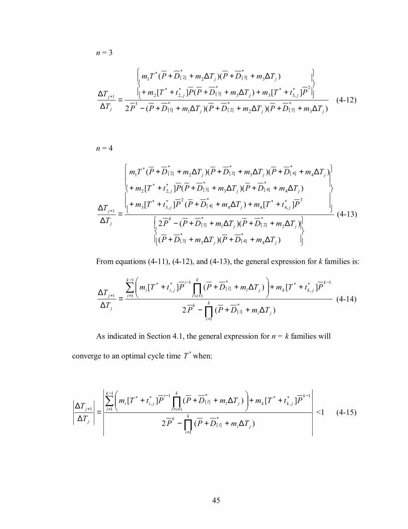
From equations (4-11), (4-12), and (4-13), the general expression for k families is:

∏

∑ ∏

=

−

=

−

+=

−

+

∆++−

++

∆+++=

∆∆

k

ijii

k

k

i

k

jkk

k

iljll

i

jii

j

j

TmDPP

PtTmTmDPPtTm

TT

1

*][

1

1

1*,

*

1

*][

1*,

*

1

)(2

][)(][ (4-14)

As indicated in Section 4.1, the general expression for n = k families will

converge to an optimal cycle time *T when:

∏

∑ ∏

=

−

=

−

+=

−

+

∆++−

++

∆+++=

∆∆

k

ijii

k

k

i

k

jkk

k

iljll

i

jii

j

j

TmDPP

PtTmTmDPPtTm

TT

1

*][

1

1

1*,

*

1

*][

1*,

*

1

)(2

][)(][<1 (4-15)

46

4.3 Convergence Example and Discussion

The general expression (4-15) is evaluated using the example problem in Section

2 of Chapter 3. Using the results from the example at the first iteration; i.e., j = 1 and at

the optimal cycle time *T , the general expression is evaluated as follows:

*T = 2.69, *

]1[D = 1038.7, *

]2[D = 936.88, *

]3[D = 1104.92,

]1[*t = 0, ]2[

*t = 0.93, ]3[*t = 1.73, P = 3000.

1T∆ = 3.47- 2.69 = 0.78

41.1178.0

7.10386.10471 =−=m , 62.43

78.088.9369.970

2 =−=m

15.2578.0

92.11043.10853 −=−=m

In this example n = 3, following the general expression:

*1Tm = (11.41) (2.69) = 30.69

][ *,2

*2 jtTm + = (43.62) (2.69 + 0.93) = 157.90

][ *,3

*3 jtTm + = (-25.15) (2.69 + 1.73) = -111.16

)( 1*

]1[ jTmDP ∆++ = 3000 + 1038.70 + (11.41) (0.78) = 4047.60

)( 2*

]2[ jTmDP ∆++ = 3000 + 936.88 + (43.62) (0.78) = 3970.90

)( 3*

]3[ jTmDP ∆++ = 3000 + 1104.92 + (-25.15) (0.78) = 4085.30

47

The convergence condition:

1))()((2

][)(][

))((

3*

]3[2*

]2[1*

]1[3

2*,3

*33

*]3[

*,2

*2

3

*]3[2

*]2[

*1

1 <∆++∆++∆++−

++∆++++

∆++∆++

=∆

∆ +

jjj

jjj

jj

j

j

TmDPTmDPTmDPP

PtTmTmDPPtTm

TmDPTmDPTm

TT

)30.4085)(90.3970)(60.4047()3000(2)3000)(16.111()30.4085)(3000)(90.157()30.4085)(90.3970)(69.30(

3

2

1

2

−−++=

∆∆

TT <1

1123.061166145340

1432629542

1

2 <−=−

=∆∆

TT

Note that the condition for the convergence is satisfied. Furthermore,

2T∆ = 01.0)123.0()78.0()123.0(1 −=−=−∆T

This result agrees with the result from the example problem in Chapter 3, where

2T∆ = 2T - *T = 2.59 – 2.69 = -0.01.

The general expression (4-15) converges when the absolute value of the

numerator is less than the absolute value of the denominator.

∏

∑ ∏

=

−

=

−

+=

−

∆++−<

++

∆+++

k

ijii

k

k

i

k

jkk

k

iljll

i

jii

TmDPP

PtTmTmDPPtTm

1

*][

1

1

1*,

*

1

*][

1*,

*

)(2

][)(][

In the above expression, P and *

][ iD are always positive values. ji Tm ∆ equal

jiD ],[∆ for all i which is a small value compared to P and *

][ iD . This concludes that the

48

term )(*

][ jii TmDP ∆++ is always positive. im can be positive or negative and relatively

large or small depending on the demand’s variation. Recall that iT

Dm

j

jii ∀

∆∆

= ,],[ .

The absolute value of the numerator depends on im as it is the only term that can

have a negative value in the numerator. Also, when some of the im s have negative values

and the others have positive values the numerator tends to be smaller. Recall that im

depends on the differences between the demands averages over the iterations which

depend on the demand variability. It is concluded that the numerator decreases when the

demand variability is decreasing, and increases when the demand variability is

increasing. In the experiments in Chapter 3, two levels of demand variability are

considered v = 0.2 and v = 0.5. In the experimental results, more data sets do not

converge to an optimal cycle time when v = 0.5 due to the higher demand variability.

In the denominator, the production rate, P is assumed to equal the summation of

the demands’ averages ∑=

k

iiD

1

*][ in each period, which without loss of generality, is equal

the number of the families multiplied by the average demand for a single family

(*

][1

*][ i

k

ii DkDP ≅≅ ∑

=). Notice that as k increases the negative part of the denominator

(∏=

∆++k

ijii TmDP

1

*][ )( ) becomes larger than the positive part (

kP2 ) and the whole

denominator increases. In the experiments in Chapter 3, three levels for the number of

families are used n = 3, n = 6, and n = 9. In the experimental results, more data sets

converge to an optimal cycle time when the number of families increases.

49

4.4 Comparison of Algorithms A1 and A1B Convergence Expressions

Yalcin and Boucher [31] provide a general convergence expression for the A1

formulation for k families as follows:

( ) 21

*]1[1

*]1[

2*,1

*11

*]1[1

))(2(

]][))(2[(−

−−−−

−−−−−+

∆++∆++−

++∆++−−=

∆∆

kjkkjkk

kjkkjkk

j

j

PTmDTmDPfamilieskfornatordenomi

PtTmTmDPfamilieskfornumeratorT

T (4-16)

When k = 3 families in equation (4-16), )2(

)2(familieskfornatordenomi

familieskfornumerator−

− forms the

seed for the expression and equals jTmD

tTm

∆+

+

1

*]1[

*1

*1 ][ . In order to get a general expression

similar to the A1B formulation general convergence expression (4-14), the seed is

substituted and further rearrangement is made to obtain the following general expression:

( ) ( )∑ ∏

∑ ∏−

=

−

−−

−

+=

−

−

=

−

−−

−

+=

−

+

∆++

∆++∆+−

++

∆+++=

∆∆

2

1

21

*]1[

1

1

*][

1*][

2

1

2*,1

*1

1

1

*][

1*,

*

1

)(

][)(][

k

i

kjkk

k

iljll

ijii

k

i

k

jkk

k

iljll

i

jii

j

j

PTmDTmDPPTmD

PtTmTmDPPtTm

TT

(4-17)

The two general convergence expressions (4-14) and (4-17) have the same

numerator patterns. However; the general convergence expression in equation (4-17) for

Algorithm A1 does not contain the last family term as the summation is up to k-2 families

only unlike the general convergence expression in equation (4-14) where it is up to k-1

families. Moreover; P is raised to the power of k-2 in equation (4-17) while it is k-1 in

equation (4-14). These two factors cause the numerator of equation (4-17) to be smaller

than the numerator of equation (4-14) for the same data set.

The denominator in equation (4-17) for Algorithm A1 contains a positive and a

negative term. However, the denominator in equation (4-14) for Algorithm A1 contain

50

only a negative term. This difference causes the denominator in equation (4-14) to have a

greater absolute value than the numerator.

Since the general convergence expression for Algorithm A1B has a larger

numerator and a smaller denominator compared to the general convergence expression

for Algorithm A1 for the same data set, it is concluded that Algorithm A1B is less

“convergent” compared to Algorithm A1 which explains the presence of data sets that

converge using Algorithm A1 but not A1B.

4.5 A Modification to Algorithm A1B and Comparison to RKM

As indicated in section 4.1 the non-convergence occurs between step 6 and 7 of

Algorithm A1B. A proposed modification is to evaluate an extra condition ( 11

≥∆∆

−j

j

TT

)

for non-convergence in step 7 after solving equation set (3-4). If the condition does not

hold then the algorithm is converging to an optimal cycle time *T . However, if it holds,

then the algorithm is not going to converge to an optimal cycle time *T by solving

equation set (3-4). Therefore, the algorithm proceeds and solves equation set (3-4a).

Note that 1−−=∆ jjj TTT , 211 −−− −=∆ jjj TTT and T0 is an estimation so at least

three iteration are needed to evaluate the condition 11

≥∆∆

−j

j

TT

. The modified step 7 is as

follows:

51

Step 7: Increment j. Solve equation set 3-4.

If j ≥ 3 then [If 11

≥∆∆

−j

j

TT

, go to step 9].

If ∆±≠ −1jj TT , go to step 6

The modification is applied to algorithm A1B to populate the missing data in

Table 3.2 where v = .5 as shown in Table 4.1. Following that the missing data in Table

3.6 is filled as shown in Table 4.2. All the comparisons in Table 4.2 are still statistically

significant above the 95% level of confidence. The results show that the number of setups

using the modified Algorithm A1B when there is a non-convergence data set is less than

the number of setups using Algorithm RKM.

Table 4.1 Paired Comparisons of Number of Setups: n = 3





25 16 11 7 11 5 20 12 12 6 11 4 20 14 12 7 11 5 19 11 12 6 12 5 17 10 12 6 10 4 19 12 12 6 12 5

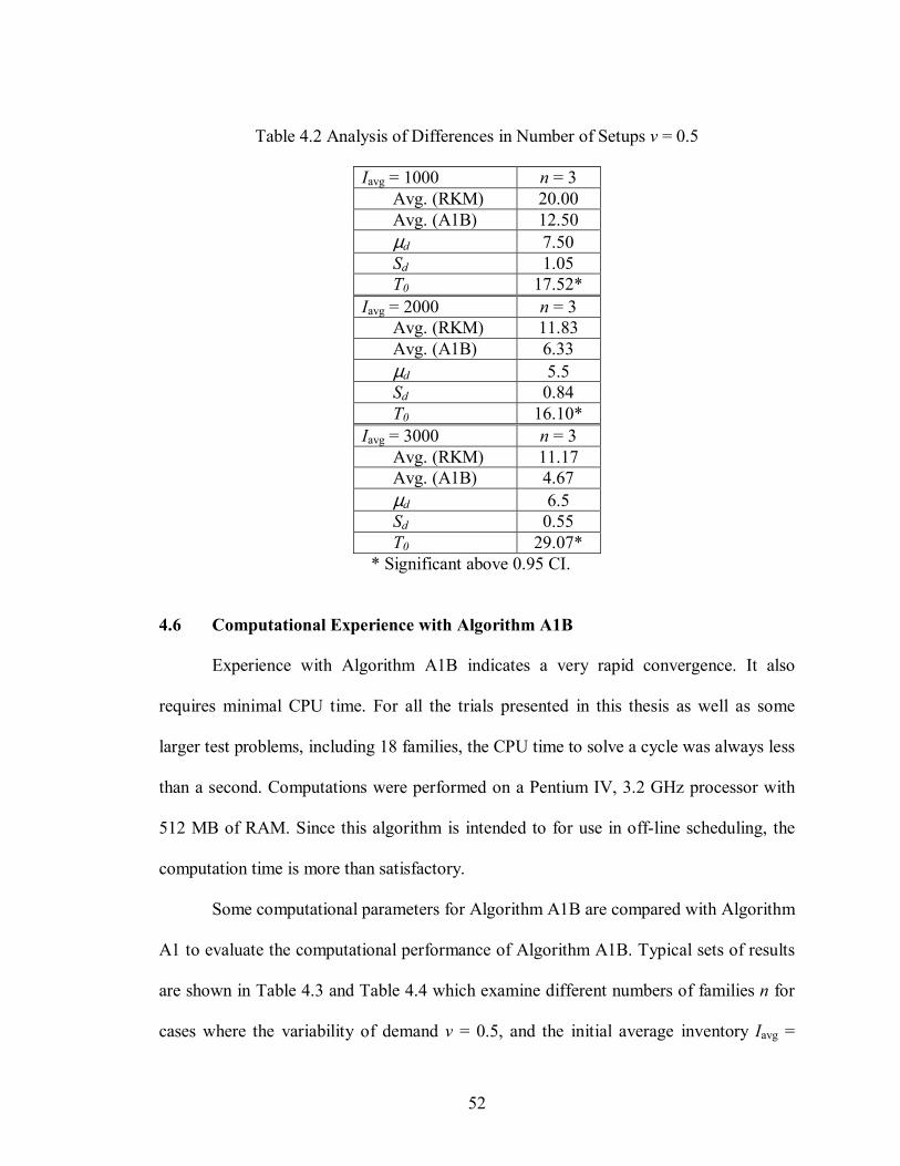
52


Iavg = 1000 n = 3 Avg. (RKM) 20.00 Avg. (A1B) 12.50 µd 7.50 Sd 1.05 T0 17.52* Iavg = 2000 n = 3 Avg. (RKM) 11.83 Avg. (A1B) 6.33 µd 5.5 Sd 0.84 T0 16.10* Iavg = 3000 n = 3 Avg. (RKM) 11.17 Avg. (A1B) 4.67 µd 6.5 Sd 0.55 T0 29.07*


4.6 Computational Experience with Algorithm A1B

Experience with Algorithm A1B indicates a very rapid convergence. It also

requires minimal CPU time. For all the trials presented in this thesis as well as some

larger test problems, including 18 families, the CPU time to solve a cycle was always less

than a second. Computations were performed on a Pentium IV, 3.2 GHz processor with

512 MB of RAM. Since this algorithm is intended to for use in off-line scheduling, the

computation time is more than satisfactory.

Some computational parameters for Algorithm A1B are compared with Algorithm

A1 to evaluate the computational performance of Algorithm A1B. Typical sets of results

are shown in Table 4.3 and Table 4.4 which examine different numbers of families n for

cases where the variability of demand v = 0.5, and the initial average inventory Iavg =

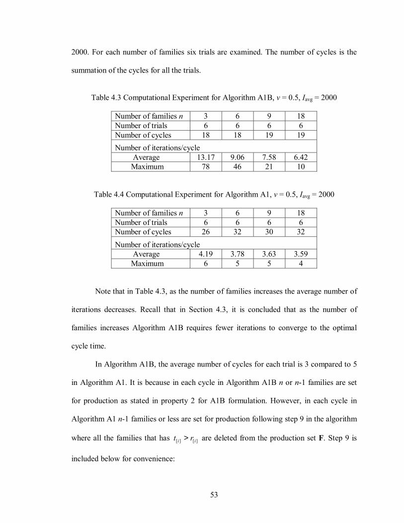
53

2000. For each number of families six trials are examined. The number of cycles is the

summation of the cycles for all the trials.

Table 4.3 Computational Experiment for Algorithm A1B, v = 0.5, Iavg = 2000

Number of families n 3 6 9 18 Number of trials 6 6 6 6 Number of cycles 18 18 19 19 Number of iterations/cycle Average 13.17 9.06 7.58 6.42 Maximum 78 46 21 10

Table 4.4 Computational Experiment for Algorithm A1, v = 0.5, Iavg = 2000

Number of families n 3 6 9 18 Number of trials 6 6 6 6 Number of cycles 26 32 30 32 Number of iterations/cycle Average 4.19 3.78 3.63 3.59 Maximum 6 5 5 4

Note that in Table 4.3, as the number of families increases the average number of

iterations decreases. Recall that in Section 4.3, it is concluded that as the number of

families increases Algorithm A1B requires fewer iterations to converge to the optimal

cycle time.

In Algorithm A1B, the average number of cycles for each trial is 3 compared to 5

in Algorithm A1. It is because in each cycle in Algorithm A1B n or n-1 families are set

for production as stated in property 2 for A1B formulation. However, in each cycle in

Algorithm A1 n-1 families or less are set for production following step 9 in the algorithm

where all the families that has ][][ ii rt > are deleted from the production set F. Step 9 is

included below for convenience:

54

Step 9: Set k = the largest number i in F for which ][][ ii rt > is true. Delete from F

all families where ki > . Go to Step 1.

As indicated in Section 4.4, the general expression for convergence of Algorithm

A1 has a smaller absolute value than the general expression for convergence of

Algorithm A1B for the same data set. This explains why the average number of iterations

per cycle in Algorithm A1B is larger than Algorithm A1 as Algorithm A1 needs fewer

iterations to converge to the optimal cycle time.

55

Chapter 5. Continuous Time Disaggregation and Demand Uncertainty

This chapter considers the demand uncertainty in the continuous time

disaggregation allowing backorder with experimental results. It is divided into 2 sections.

Section 5.1 incorporate demand uncertainty into Algorithm A1B, and compares the

performance of Algorithm A1B in the presence of demand uncertainty and Algorithm

A1B with deterministic demand. Section 5.2 incorporates a desired service level

parameter into the problem formulation and Algorithm A1B.

5.1 Algorithm A1B in the Presence of Demand Uncertainty

Allowing backorders in HPP’s disaggregation step allows incorporating demand

uncertainty into the problem formulation and solution. Demand uncertainty is

incorporated into the problem assuming that the actual demands are known at the

beginning of each period. Demand for each family is assumed to be an independent

random variable which follows a specific distribution and only the information about

demand’s mean and variation is known for the remainder of the planning horizon.

Since it is assumed that actual demands become available at the beginning of each

period, the time when Algorithm A1B is set to run again is an important consideration.

The policy proposed here is to check if there is any new actual demand information

before changing over between the families. If there is new information then the algorithm

is run again before a change-over is performed and the next family starts its production.

56

This policy keeps the algorithm updated with the new demand information

without interfering with its continuous behavior. Another policy is set the algorithm to

run again whenever there is new demand information. Since it is assumed that the actual

demands become available at the beginning of each period, this policy sets the algorithm

to run at the beginning of each period converting the algorithm from a continuous time to

a discrete time algorithm.

The experimental design in Chapter 3 is used again to evaluate the effectiveness

of using Algorithm A1B in the presence of demand uncertainty. In Chapter 3, three

control parameters are used to generate different data sets for the experiment. These

parameters are: the number of families n with three levels: three, six and nine, the amount

of the average initial inventory Iavg with three levels: one, two and three periods of

supply, and the demand variability v with two levels: high variability (0.5) and low

variability (0.2).

The algorithm is compared with Algorithm A1B with deterministic demand based

on the percentage of the time of each family is out-of-stock during the entire planning

horizon as shown in Table 5.1.

Table 5.1 Paired Comparison of Out-of-stock Percentage

n = 3

n = 6 n = 9

v 0.2 0.5 0.2 0.5 0.2 0.5 Iavg = 1000 A1B deterministic 1.97% 4.06% 2.55% 5.80% 2.48% 5.16% A1B uncertain demand 3.00% 5.22% 4.39% 7.85% 3.89% 6.79% Iavg = 2000 A1B deterministic 1.38% 3.04% 1.41% 3.62% 1.34% 2.74% A1B uncertain demand 2.86% 6.26% 2.79% 5.16% 2.25% 4.31% Iavg = 3000 A1B deterministic 1.12% 1.99% 1.44% 3.03% 1.40% 2.88% A1B uncertain demand 1.87% 4.52% 1.92% 4.43% 1.64% 3.28%

57

The results show that the averages of percentage of time each family is out-of-

stock during the entire planning horizon in the presence of demand uncertainty are

greater than those with deterministic demands patterns for all data sets. A one-tail test

statistic is constructed to check the significant of the results of Table 5.1. The test statistic

for one-tail test with 17 degree of freedom and a 99% confidence interval is 2.567. The

test results show that the comparisons in Table 5.1 are statistically significant above the

99% confidence interval as shown in Table 5.2. These results are expected as the demand

uncertainty tends to increase the time the family is out-of-stock. Furthermore, it confirms

that the incomplete knowledge of the demand decrease the service level associated with

the families, highlighting the importance of the decision associated with when Algorithm

A1B should be re-run.

Table 5.2 Analysis of Differences in Out-of-stock Percentage

Avg. (A1B deterministic demand) 2.63% Avg. (A1B uncertain demand) 4.02% µd 1.39% Sd 0.01 T0 7.95


As stated in Chapter 3, two levels of demand variability are used in the

experimental design: low variability v = 0.2 and high variability v = 0.5. Based on the

data in Table 5.1, a one-tail test statistics is constructed to check the effect of the demand

variability on the percentage of the time of each family being out-of-stock during the

entire planning horizon. The test statistic for one-tail test with 8 degree of freedom and a

99% confidence interval is 2.896. Table 5.3 shows the results of the one-tail test which

states that, as the demand variability increases, the difference between the percentage of

out-of-stock time during the entire planning horizon between Algorithm A1B in the

58

presence of demand uncertainty and Algorithm A1B with deterministic demand

increases. This result shows that families with high actual demand variability have poorer

service level than families with low demand variability.

Table 5.3 Analysis of Differences Based on Demand Variability

Avg. (v = 0.2) 1.06% Avg. (v = 0.5) 1.72% µd 0.66% Sd 0.01 T0 2.93*


5.2 Incorporating a Service Level Parameter in the Problem Formulation

In Section 5.1, the experimental results show that demand uncertainty decreases

the service levels associated with the families and show that families with higher actual

demand variability has poorer service level. In this section, a service level parameter

associated with the production characteristic and the importance of satisfying the demand

of each family is introduced. The service level parameter is incorporated in the problem

formulation as follows:

TMax , (5-1a)

s.t. [ ] )1...(2,1,01][][ ][][][][][]1[0],[ −=≥++−−+ + niDZTtPttI iiiiiii , (5-1b)

[ ] niDZTtPtTI iiiiii =≥++−−+ ,01][][ ][][][][][0],[ , (5-1c)

where ][iZ is a constant and equal to ][][ ii vc where:

][ic is the coefficient of variation of the ith product family in the production cycle,

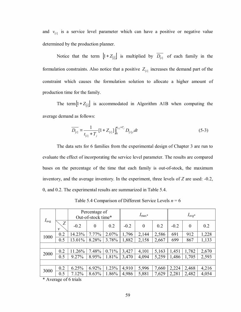
59

and ][iv is a service level parameter which can have a positive or negative value

determined by the production planner.

Notice that the term [ ][ ]iZ+1 is multiplied by ][iD of each family in the

formulation constraints. Also notice that a positive ][iZ increases the demand part of the

constraint which causes the formulation solution to allocate a higher amount of

production time for the family.

The term [ ][ ]iZ+1 is accommodated in Algorithm A1B when computing the

average demand as follows:

∫+

++

= ji Tt

tiiji

i dtDZTt

D ][

0 ],[][][

][ ]1[1 (5-3)

The data sets for 6 families from the experimental design of Chapter 3 are run to

evaluate the effect of incorporating the service level parameter. The results are compared

bases on the percentage of the time that each family is out-of-stock, the maximum

inventory, and the average inventory. In the experiment, three levels of Z are used: -0.2,

0, and 0.2. The experimental results are summarized in Table 5.4.

Table 5.4 Comparison of Different Service Levels n = 6

Percentage of Out-of-stock time* Imax* Iavg*

Iavg Z v -0.2 0 0.2 -0.2 0 0.2 -0.2 0 0.2

0.2 14.23% 7.77% 2.07% 1,796 2,144 2,586 691 912 1,228 1000 0.5 13.01% 8.28% 3.78% 1,882 2,158 2,667 699 867 1,133

0.2 11.26% 7.48% 0.71% 3,427 4,101 5,163 1,451 1,782 2,670 2000 0.5 9.27% 8.95% 1.81% 3,470 4,094 5,259 1,486 1,705 2,593

0.2 6.25% 6.92% 1.23% 4,910 5,996 7,660 2,224 2,468 4,216 3000 0.5 7.12% 8.63% 1.86% 4,986 5,881 7,629 2,281 2,482 4,054 * Average of 6 trials

60

Table 5.4 shows that increasing Z[i] associated with family i, decreases the

percentage of the time the family is out-of-stock as more production time is allocated to

the family. However; allocating more production time also increases the maximum and

the average inventory of the family.

An interesting observation is that the increase in the initial inventory does not

have any significant affect on the percentage of the time the family is out-of-stock

although it increases the maximum and average inventory of the families. Also, notice

that the demand variability does not have any effect on the experimental results.

Figures 5.1, 5.2 and 5.3 show an inventory versus time graphs for two families

with different service level parameters. In Figure 5.1, Z = 0 is used for both of the

families. In Figure 5.2, Z = -0.2 is used for one family and Z = 0.2 is used for the other

one. Then, In Figure 5.3, Z = -0.5 and Z = 0.5 are used. The inventory increase in the

graphs portions with positive slope represents the duration when this family is in

production.

Note that as Z increases the family average and maximum inventory increases.

Furthermore; the percentage of time the family is out-of-stock increases when Z

decreases. This clearly shown in Figure 5.3 where the family with Z = 0.5 has a

maximum inventory of 8000 compared to only 2000 for the family with Z = -0.5.

Also, notice that in Figure 5.1, when both of the families have the same service

level parameters, they have almost the same amount of time assigned for production

during each setup and the same number of setups. In figure 5.2, the time assigned for

production during each setup for the family with greater Z is increased while it is

decreased for the other family. This is more obvious in Figure 5.3, where the increase in

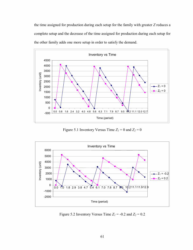
61

the time assigned for production during each setup for the family with greater Z reduces a

complete setup and the decrease of the time assigned for production during each setup for

the other family adds one more setup in order to satisfy the demand.

Figure 5.1 Inventory Versus Time Z1 = 0 and Z2 = 0

Figure 5.2 Inventory Versus Time Z1 = -0.2 and Z2 = 0.2

Inventory vs Time

-500

0

500

1000

1500

2000

2500

3000

3500

4000

4500

0.0 0.8 1.6 2.4 3.2 4.0 4.8 5.6 6.3 7.1 7.9 8.7 9.5 10.2 11.1 12.0 12.7

Time (period)

Inve

ntor

y (u

nit)

Z1 = 0Z2 = 0

Inventory vs Time

-2000

-1000

0

1000

2000

3000 4000 5000 6000

0.0 1.0 1.8 2.9 3.8 4.7 5.4 6.1 7.0 7.8 8.7 9.3 10.211.111.912.9

Time (period)

Inve

ntor

y (u

nit)

Z1 = -0.2Z2 = 0.2

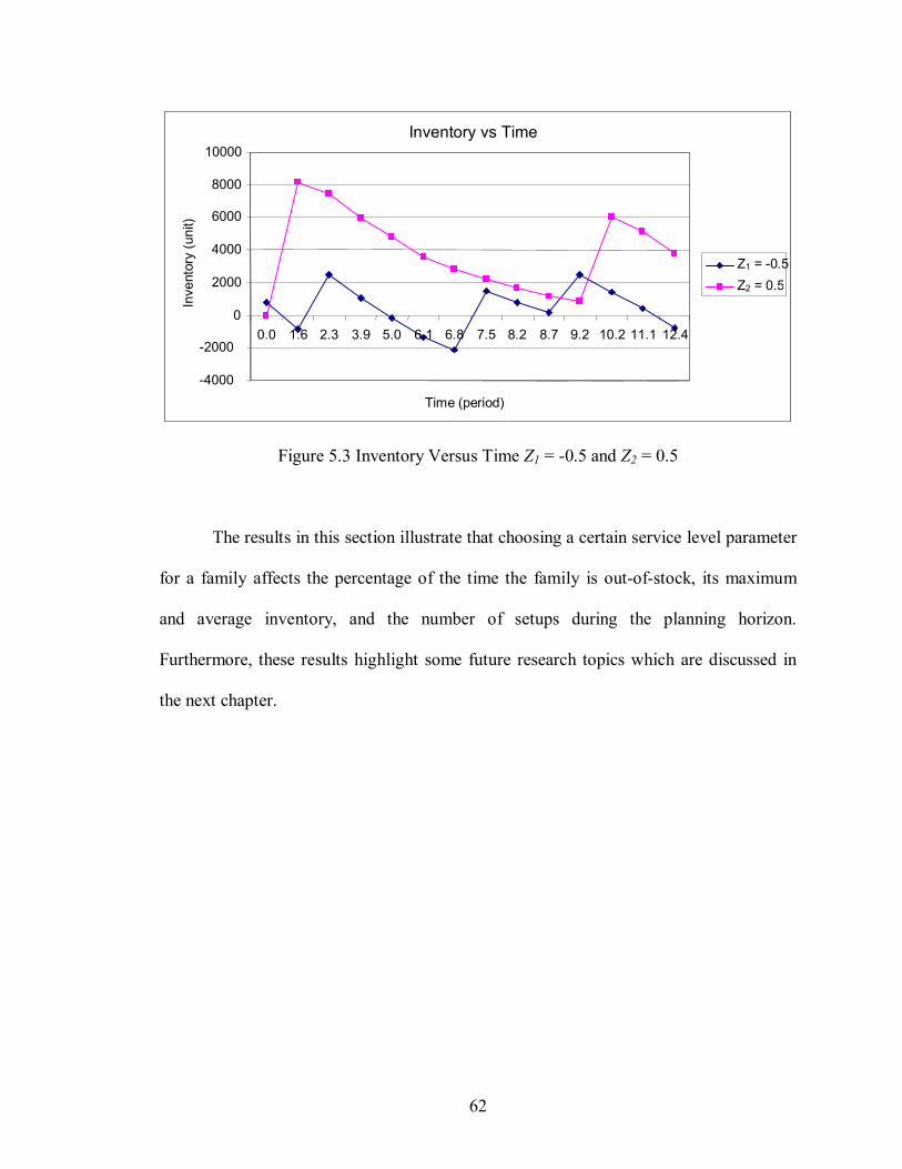
62

Figure 5.3 Inventory Versus Time Z1 = -0.5 and Z2 = 0.5

The results in this section illustrate that choosing a certain service level parameter

for a family affects the percentage of the time the family is out-of-stock, its maximum

and average inventory, and the number of setups during the planning horizon.

Furthermore, these results highlight some future research topics which are discussed in

the next chapter.

Inventory vs Time

-4000

-2000

0

2000

4000

6000

8000

10000

0.0 1.6 2.3 3.9 5.0 6.1 6.8 7.5 8.2 8.7 9.2 10.2 11.1 12.4

Time (period)

Inve

ntor

y (u

nit)

Z1 = -0.5Z2 = 0.5

63

Chapter 6. Conclusions and Future Work

This chapter summarizes the results and the conclusions of the thesis and outlines

the directions for further research. Section 6.1 summarizes the results and the conclusions

derived from this research. Section 6.2 presents the directions for future research in the

continuous time disaggregation area.

6.1 Conclusions

This thesis extends the continuous-time disaggregation approach for hierarchical

production planning introduced by Yalcin and Boucher [31]. To the best of our

knowledge, the algorithm presented in this thesis is the only continuous algorithm that

allows backorder and considers demand uncertainty.

In Chapter 3, a continuous-time disaggregation formulation that allows backorder

is provided and an algorithm (Algorithm A1B) based on this formulation is presented. At

the end of Chapter 3, a design of experiment is used to show the effectiveness of the

Algorithm A1B over the Regular Knapsack Method Algorithm [6] in reducing the

number of setups, and to demonstrate how allowing backorder eliminates the

compression effect problem presented in [31].

Chapter 4 discusses the convergence conditions and computational requirements

associated with Algorithm A1B. A general expression for convergence is obtained. It is

64

concluded that increasing the number of families and decreasing the demand variability

allows Algorithm A1B to converge to an optimal cycle time more readily. A comparison

for convergence conditions and other computational requirements of the Algorithm A1B

and Algorithm A1 presented in [31] shows that Algorithm A1B has more strict

convergence conditions compared Algorithm A1. Finally, a modification to detect and

resolve the non-convergence data sets is introduced for Algorithm A1B.

Chapter 5 incorporates demand uncertainty into continuous-time disaggregation.

The experimental results confirm that uncertainty associated with demand increases the

percentage of the time the family is out of stock leading to decrease service levels. A

family service level parameter which can be used to capture the production planners’

desired risk-level of being out-of-stock for each family is introduced. Experiments show

that service level parameter for a family can be effectively used to decrease the

percentage of the time the family is out-of-stock.

In the disaggregation process, the measure of efficiency is the minimization of the

number of setups during the planning horizon. The results of this thesis show that

continuous-time disaggregation allowing backorder approach is effective over discrete-

time disaggregation approaches in minimizing the number of setups. From industry

application perspective, where the setup costs are high, the continuous-time

disaggregation can be very useful in minimizing the costs and incorporating demand

uncertainty.

The experimental results in this thesis were designed using constant production

rates and uniform demand distribution for simplicity. However continuous-times

65

disaggregation can cope with variable production rates and other demand distribution that

might exist in industry applications.

6.2 Future Work

The presented continuous time disaggregation is considered at the disaggregation

done at the family level of HPP. A future research direction can extend this research to

consider the disaggregation done at the items levels.

A future research can consider a formal proof associated with the detection of

non-convergence. Possibly, to check the demand patterns of the data set before starting

the disaggregation process.

It is concluded that the time when to set the algorithm to run again in the presence

of demand uncertainty is an important consideration. A future study can reconsider the

time when new demand information is available to study different policies for the time

when the algorithm is set to run again.

The service level parameter introduced in Chapter 5 could be implemented in a

real world application. The families preferred specifications set by the planners such as

aimed average inventory, maximum and minimum inventory allowed and percentage of

time the family is out-of-stock can be used to derive the service level parameter for each

family. Furthermore, as the service level parameter affects the number of setups

associated with each family, this research can also be extended to include the situation

when different setup costs are associated when changing over between the families.

66

References

[1] Askin, R.G. and J.B. Goldberg (2002) Design and analysis of lean production

systems, Wiley, New York, NY, 130-164. [2] Akturk, M.S. and G.R Wilson (1998) A hierarchical model for the cell loading

problem of cellular manufacturing systems. International Journal of Production Research, 36, 2005-2023.

[3] Ari, E. A. and S. Axsater (1988) Disaggregation under uncertainty in hierarchical

production planning. European Journal of Operational Research, 35, 182-186. [4] Axsater, S. (1981) Aggregation of product data for hierarchical production,

Operations Research, 29, 744-755. [5] Bitran, G. R. and A. C. Hax (1977) On the design of hierarchical production

control systems, Decision Science, 8, 28-55. [6] Bitran, G. R. and A. C. Hax (1981) Disaggregation and resource allocation using

convex knapsack problems with bounded variables, Management Science, 27, 431-441.

[7] Bitran, G. R., E. A Hass, and A. C. Hax (1981) Hierarchical production planning:

a single stage system, Operations Research, 29, 717-743. [8] Bitran, G. R., E. A Hass, and A. C. Hax (1982) Hierarchical production planning:

a two stage system, Operations Research, 30, 232-251. [9] Bitran, G. R., E. A Hass, and H. Matsuo (1986) Production planning of style

goods with high setup costs and forecast revisions, Operations Management, 34, 226-236.

[10] Ciarallo, F.W., R. Akella, and T.E. Morton (1994) A periodic review, production

planning model with uncertain capacity and uncertain demand-optimality of extended myopic policies. Management Science, 40, 320-332.

[11] Dempster, M. A. H.; Fisher, M. L., Jansen, L. Jansen; Lageweg, B. J., Lenstra, J.

K., and Rinnooy Kan, A. H. G. (1981), Analytical evaluation of hierarchical planning systems. Operations Research, 29, 707-716.

67

[12] Erschler, J., G. Fontan, and C. Merce (1986) Consistency Of the disaggregation process in hierarchical production planning, Operations Research, 34, 464-469.

[13] Gfrerer, H and G. Zapfel (1995) Hierarchical model for production planning in

the case of uncertain demand, European Journal of Operational Research, 86, 142-161.

[14] Graves, S.C. (1982) Using Lagrangean techniques to solve hierarchical

production planning problems, Management Science, 28, 260-275. [15] Hax, A. C. and H. C. Meal (1975) Hierarchical integration of production planning

and scheduling, Studies in Management Sciences, Volume 1: Logistics, North-Holland, Amsterdam, 53-69.

[16] Kasilingam, R.G. (1995) Product mix determination in the presence of alternate

process plans and stochastic demand. Computers Industrial Engineering, 29, 249-253.

[17] Karmarkar, N. (1984) A new polynomial time algorithm for linear programming.

Comniatorica, 4, 373-395. [18] Kira, D., M. Kusy, and I. Rakita (1997) A Stochastic Linear Programming

Approach to Hierarchical Production Planning. Journal of the Operational Research Society, 48, 2, 207-211.

[19] Lasserre, J.B., and C. Merce (1990) Robust hierarchical production planning

under uncertainty. Annals of Operations Research, 26, 73-87. [20] Matsuo, H (1990) A stochastic sequencing problem for style goods with forecast

revisions and hierarchical structure. Management Science, 36, 332-347. [21] Montgomery, D.C. (2001) Design and Analysis of Experiment, John Wiley &

Sons, New York, NY. [22] Mulvey, J.M. and A. Ruszczynski (1995) A new scenario decomposition method

for large-scale stochastic optimization. Operations Research, 43, 477-490. [23] Nahmias, S. (2005) Production and Operations Analysis, McGraw-Hill, New

York, NY. [24] Neureuther, B.D., G.G. Polak, and N.R. Sanders (2004) A hierarchical production

plan for a make-to-order steel fabrication plant. Production Planning & Control, 15, 324-335.

68

[25] Nguyen, P.L. and L. Dupont (1993), Production management of a steel manufacturing system: a hierarchical planning model. Computers and Industrial Engineering, 25, 81-84.

[26] Ozdamar, L., A.O. Atli, and M.A. Bozyl (1996) Heuristic family disaggregation

techniques for hierarchical production planning systems. International Journal of Production Research, 35, 2613-2628.

[27] Qui, M.M. and E.E. Burch (1997) Hierarchical production planning and

scheduling in a multi-product, multi-machine environment. International Journal of Production Research, 35, 3023-3042.

[28] Qui, M.M., L.D. Fredendall, and Z. Zhu (2001) Application of hierarchical

production planning and scheduling in a multiproduct, multimachine environment. International Journal of Production Research, 39, 2803-2816.

[29] Saad, G.H. (1990) Hierarchical production planning systems: extensions and

modifications. The Journal of the Operational Research Society, 41, 609-624. [30] Tsubone, H. and M. Sugawara (1987) A hierarchical production planning sstem in

motor industry. OMEGA, 15, 113-120. [31] Yalcin, A. and T. O. Boucher (2004) A continuous-time algorithm for

disaggregation under uncertainty of hierarchical production plans, IIE Transactions, 35, 1023-1035.

[32] Yan, H.S. (2000) Hierarchical stochastic production planning with delay

interaction. Journal of Optimization Theory and Applications, 104, 659-689. [33] Yan, H.S. (2000) Hierarchical stochastic production planning for flexible

automation workshops. Computers & Industrial Engineering, 38, 435-455. [34] Yan, H.S. (2001) Hierarchical stochastic production planning for the highest

business benefit. Robotics and Computer Integrated Manufacturing, 17, 405-419. [35] Yan, H.S. (2003) Practical solution approached to solve a hierarchical stochastic

production planning problem in a flexible automated workshop in China. IIE Transactions, 35, 103-115.

[36] Yan, H., and Q. Zhang (1997) A numerical method in optimal production and

setup scheduling of stochastic manufacturing systems. IIE Transactions on Automatic Control, 42, 1452-1455.

[37] Yin, K.K., G.G. Yin, and H. Liu (2004) Stochastic modeling for inventory and

production planning in the paper industry. AIChE Journal, 50, 2877-2890.

69

[38] Yokoyama, M. and H.W. Lewis III (2003) Optimization of stochastic cycling problem by genetic algorithm. Computers & Operations Research, 30, 1831-1849.

continuous time disaggregation in hierarchical production

Documents