continuously differentiable selections and
TRANSCRIPT

Louisiana State UniversityLSU Digital Commons
LSU Historical Dissertations and Theses Graduate School
1995
Continuously Differentiable Selections andParametrizations of Multifunctions in OneDimension.Craig KnucklesLouisiana State University and Agricultural & Mechanical College
Follow this and additional works at: https://digitalcommons.lsu.edu/gradschool_disstheses
This Dissertation is brought to you for free and open access by the Graduate School at LSU Digital Commons. It has been accepted for inclusion inLSU Historical Dissertations and Theses by an authorized administrator of LSU Digital Commons. For more information, please [email protected].
Recommended CitationKnuckles, Craig, "Continuously Differentiable Selections and Parametrizations of Multifunctions in One Dimension." (1995). LSUHistorical Dissertations and Theses. 5962.https://digitalcommons.lsu.edu/gradschool_disstheses/5962

INFORMATION TO USERS
This manuscript has been reproduced from the microfilm master. UMI films the text directly from the original or copy submitted. Thus, some thesis and dissertation copies are in typewriter face, while others may be from any type of computer printer.
The quality of this reproduction is dependent upon the quality of the copy submitted. Broken or indistinct print, colored or poor quality illustrations and photographs, print bleedthrough, substandard margins, and improper alignment can adversely affect reproduction.
In the unlikely event that the author did not send UMI a complete manuscript and there are missing pages, these will be noted. Also, if unauthorized copyright material had to be removed, a note will indicate the deletion.
Oversize materials (e.g., maps, drawings, charts) are reproduced by sectioning the original, beginning at the upper left-hand comer and continuing from left to right in equal sections with small overlaps. Each original is also photographed in one exposure and is included in reduced form at the back of the book.
Photographs included in the original manuscript have been reproduced xerographically in this copy. Higher quality 6" x 9" black and white photographic prints are available for any photographs or illustrations appearing in this copy for an additional charge. Contact UMI directly to order.
UMIA Bell & Howell Information Company
300 North Zeeb Road, Ann Arbor, Ml 48106-1346 USA 313/761-4700 800/521-0600


CONTINUOUSLY DIFFERENTIABLE SELECTIONSAND
PARAMETRIZATIONS OF MULTIFUNCTIONSIN
ONE DIMENSION
A Dissertation
Submitted to the Graduate Faculty of the Louisiana State University and
Agricultural and Mechanical College in partial fulfillment of the
requirements for the degree of Doctor of Philosophy
in
The Department of Mathematics
byCraig Knuckles
B.S., Tennessee Technological University, 1989 M.S., Tennessee Technological University, 1991
May 1995

UMI Number: 9538742
UMI Microform 9538742 Copyright 1995, by UMI Company. All rights reserved.
This microform edition is protected against unauthorized copying under Title 17, United States Code.
UMI300 North Zeeb Road Ann Arbor, MI 48103

ACKNOWLEDGEMENTS
The author would like to thank his advisor, Dr. Peter Wolenski, for working
patiently with him and providing many valuable insights into Mathematics. He
especially thanks Dr. Wolenski for helping him with the preparation of this disser
tation. The author would also like to thank Dr. John Hildebrant, Dr. Guillermo
Ferreyra, Dr. Gerald Knapp, Dr. Frank Neubrander, and Dr. Robert Perlis for
serving on his committee.
In a much different respect, the author offers profound thanks to his parents Mr.
and Mrs. Otis Knuckles. As a youth, they provided him the proper environment in
which to instill the fortitude necessary for success in a long collegiate career. Their
financial support made surviving a ten year collegiate career possible. They also
continually provided him with moral support and encouragement. The author feels
that it would be impossible to have better parents. He would like to thank his wife
Hope Knuckles for being continually supportive throughout his graduate studies.
The author would also like to thank several long term friends Bryan Moore, Steve
Grodrian, Danny Jones, and Luther Johnson for their encouragement along the
way. Finally, the author would like to thank the band Black Sabbath for providing
most excellent contemplative music during his periods of reclusive mathematical
cogitation.
TABLE OF CONTENTS
ACKNOWLEDGEMENTS.............................................................................................. ii
INDEX OF DEFINITIONS............................................................................................ iv
ABSTRACT ......................................................................................................................v
CHAPTER
1 INTRODUCTION ............................................................................................... 1
2 DEFINITIONS AND PRELIMINARY DISCUSSION.................................. 9
3 STATEMENTS OF THE MAIN RESULTSAND SOME EXAMPLES ................................................................................26
4 PROOF OF THEOREM 3.1 ........................................................................... 32Proof of Theorem 3.1 .................................................................................. 38
5 PROOF OF THEOREM 3.2 ........................................................................... 48Proof of Theorem 3.2 (sufficiency) ............................................................ 48Proof of Theorem 3.2 (necessity) ...............................................................62
BIBLIOGRAPHY................... 63
VITA 64

1
2
3
4
5
6
7
8
9
10
11
12
13
14
15
16
INDEX OF DEFINITIONS
Multifunction (Closed, Compact, Lipschitz, e tc .) . . .
Selection (Measurable, Continuous, C 1, etc .)...........
Hamiltonian....................................................................
Parametrization (Measurable, Continuous, C 1, etc.)
Lipschitz Function.........................................................
Directional Derivative..................................................
Generalized Directional Derivative.............................
Clarke Generalized Gradient.......................................
Lower-C& Function ................................................
(Strictly) Submonotone Multifunction.....................
Subdifferentially Regular Function............................
Upper Semi-continuous Function.............................. .
Directional Convergence of Sequence.........................
Semismooth Function.................................................. .
Support Function of Convex Set................................
Left and Right Derivatives...........................................
iv

ABSTRACT
Sufficient conditions are given for a multifunction (set-valued function) to admit
a continuously differentiable selection in one dimension. These conditions are given
in terms of Clarke generalized gradients of the Hamiltonian associated with the
multifunction. Also, the multifunctions in one dimension that can be parametrized
with continuously differentiable functions are completely characterized. The char
acterization is again in terms of Clarke generalized gradients of the Hamiltonian
associated with the multifunction.

CHAPTER 1
INTRODUCTION
A multifunction (set-valued mapping) F : Rn =4 Rn is a function mapping a
point of Rn to a subset of Rn. The double arrows indicate that F takes on as
values, subsets of Rn rather than only single points as is the case with ordinary
functions. Multifunctions are playing an increasingly important role in mathemat
ics, and particularly in applications to optimal control theory. This is due to the
fact that optimal control problems can be reformulated into a so-called differential
inclusion problem, which we next briefly describe. Loosely speaking, a differential
inclusion is a generalization of an ordinary differential equation in which the right-
hand side of the equation is replaced by a multifunction. Consider the ordinary
differential equation
(ODE) x'(s) = <j)(s,x(s)) for almost all s € [0,T],
x(0) = x0,
where <f>: [0, T] x E" 4 Rn is a function usually assumed to have some continuity
properties in x and at least measurability in s. Here x'(s) denotes the derivative of
x(-) at s. A solution of the ordinary differential equation is an absolutely continuous
function x(-) satisfying the differential equation and the initial condition x(0) = x q .
A differential inclusion has the form
(DI) x;(s) 6 F(x(s)) for almost all s 6 [0,T],
x(0) = Xq ,
where F : Mn =} Kn is a multifunction.
1

A solution s(-) of (DI) is an absolutely continuous function whose derivative x'(s)
lands in the set F (x(s)) for almost all s, and which satisfies the initial condition
x(0) = xq. We briefly demonstrate the relationship between optimal control systems
and differential inclusions.
Consider a control system, which we formulate as
(CS) x ^ s ) = <f)(x(s),u(s)) for almost every s E [0,T],
u(s) E U for almost every s E [0,T],
a;(0) = a;0.
Here the control function u(-) : [0,T] —> Rm is taken to be measurable with almost
all of its values in a predetermined control set U C Rm, <j) : Rn x Rm —> Rn is a given
function (at least continuous), and x (•) : [0,T] —> Rn is the absolutely continuous
function satisfying the resulting ordinary differential equation (which is of the form
(ODE) once u(‘) has been fixed).
An equivalent and sometimes preferable manner to approach the control system
is by studying the related differential inclusion system, in which we define
F (x) = {<p{x,u) : u E U ) . (1.1)
Note that the control variables are then explicitly suppressed in the differential in
clusion formulation; they do, however, determine the structure of the multifunction
F. Under very mild and reasonable hypotheses, the (DI) and (CS) formulations
are equivalent in the sense that both models generate the same trajectories x(-).
If the pair (rc(-), w(-)) satisfies (CS), then it is trivial to see that x(') solves (DI).
The converse is not so obvious, but is nevertheless true. Namely, if x(-) solves
(DI), then there exists a measurable function u(<) so that (»(•),?/(•)) satisfies (CS).
This result follows by applying a so-called measurable selection theorem, which

3
in this context is usually referred to as Filippov’s Lemma. W hat this amounts to
is the following. Let x(-) be a solution of (DI) with F as in (1.1). If we define
V(s) = {u € U : x'{s) = (j>(x,u) for a.e. s G [0,T]}, then V(*) is another multi
function, and the sought-after control function ti(*) is a measurable function such
that u(s) G V(s) for a.e. s G [0,T]. If such a «(•) exists, then the pair (a:(*),tt(‘))
satisfies (CS). The function u(-) is an example of a measurable selection of the mul
tifunction V(*), and Filippov’s Lemma amounts to providing hypotheses for when
such selections exist.
To see why (DI) may be preferable to (CS), let us consider a Mayer-type optimal
control problem. This has the form
minimize l(x(T))
over absolutely continuous functions s(-) satisfying (CS), where Z : Rn —> R is a
predetermined function. As demonstrated above, under suitable hypotheses the
(CS) and (DI) systems have the same trajectories, and since Z is being minimized
only over the endpoints of these trajectories, the explicit nature of the control
functions play no essential role. In fact, in a theoretical sense they can complicate
the analysis because it is difficult in general to immediately determine if there is
a pair (a:(-), u(-)) which provides the minimum. On the other hand, using (DI) as
dynamics, and making the assumptions that F is compact and convex, one can
deduce the existence of optimal solutions. Thus, it can be shown that solutions
to the x’eformulation exist if F is defined as in (1.1) and F(x) is replaced by the
closed convex hull of F(x) for each x (here the nature of the control set U and the
continuity of <j> usually imply that F(x) is also bounded for each a:). Let us then
note that the compactness and convexity of the values of F, especially as they arise
in the context of control theory, is quite a natural assumption. But they are also
natural for our purposes, as we shall see.

The study of multifunctions in their own right (not necessarily arising from con
trol theory) has since become extensive. In fact, much mathematical literature has
been devoted to multifunctions in general. A large portion of this attention has
been devoted to finding selections and parametrizations of multifunctions under
various hypotheses (selections and parametrizations are defined below). The ad
vent of much of this attention was highlighted by E. Michael’s continuous selection
theorem [10] in 1956. As optimal control theory burgeoned in the 1960’s, the study
of multifunctions in general became more popular. But we now turn our attention
away from control theory and focus on the general notion of a multifunction.
Let F : Rn =3 Rn be a multifunction. The multifunction F is nonempty, closed,
compact, or convex if at each x G Rn, the set F(x) is nonempty, closed, compact,
or convex, respectively. The multifunction F : Rn =3 Rn is Lipschitz on S C Rn
if there exists a positive scalar K such that for all x \ ,x 2 G S and all 6 G F (xi),
there exists £2 € F (x2) such that
1 6 - 6 1 < K \x x - x 2\.
The multifunction F is locally Lipschitz at x if there is a neighborhood of x on which
F is Lipschitz. We mention parenthetically that Lipschitzian properties and other
properties regarding continuity of multifunctions can also be formulated using the
Hausdorff metric, which is a metric on the compact subsets of Rn (see, for example,
[1]). A multifunction F : Rw =4 R is locally bounded if for every xq e Rn, there
exist e > 0 and M > 0 such that \x — a?o| < e implies that |f/| < M for all y G F(x).
A thorough exposition of multifunctions can be found in [1].
A function / : Rn -> Rn is a selection of the multifunction F if f ( x ) G F (x) for
each x. The function / is respectively a measurable selection, continuous selection,
C 1 selection, etc., if the function / is measurable, continuous, C 1, etc. Let F : R ^ t
R be a Lipschitz multifunction, which throughout will be assumed to have compact

convex values. Our first main result, Theorem 3.1, provides sufficient conditions for
F to admit a C 1 selection.
There is an extensive literature on selection theorems for multifunctions, but to
our knowledge, there are no results giving conditions for a smooth (i.e. C 1) selection.
On the other hand, the existing results can be obtained in quite general spaces. For
example, Michael’s Continuous Selection Theorem [10] is valid for F being defined
on a complete metric space and mapping into the subsets of a Banach space. Note
that F is required to be compact and convex in Michael’s Continuous Selection
Theorem. Similar general hypotheses are sufficient for many of the measurable-
type selection theorems, as illustrated by the book by Castaing and Valadier [3],
the survey by Wagner [18], and the many references contained therein. A highly
readable treatment of the finite-dimensional case is given by Rockafellar [13]. There
is also a Caratheodory-type selection result due to Lojasiewicz [8]. A Caratheodory
function is a function / : M x K" 4 l n such that f{ - ,x ) is measurable for each
x € Rn and /(£, •) is continuous for each t S R. The book of Aubin and Frankowska
[1, Chapter 9] provides an excellent reference to these results, as well as to the
parametrization results alluded to below.
A common method used to obtain the selections mentioned above is to obtain a
sequence of approximate selections and then take a limit to obtain a selection with
the desired properties. Mere generalizations of this approach do not seem to be
adequate in obtaining a smooth selection of a multifunction, for the C l conclusion
is difficult to obtain by a limiting argument. Our proof is based upon a discretization
procedure, followed by an elaborate patching together of the pieces. (This helps to
explain why the results are framed only in dimension one, where such discretizing
and pasting is more readily realizable). Moreover, it is not a priori clear exactly
which multifunctions should have C 1 selections, since there is no obvious set-valued
analogue of classical differentiability; obviously, if the values of the multifunction

F should “collapse” to a singleton on some neighborhood J, then F , viewed as an
ordinary function, must be C 1 in the classical sense on L The term “singleton”
refers to a set consisting of a single point.
The Hamiltonian H of a multifunction F is given by
H (x,p) = sup{(v,p) : v e F{x)}.
Our first main result, Theorem 3.1, asserts that if the Clarke gradient (defined in
Chapter 2) of the Hamiltonian H associated with F is submonotone in the sense of
Spingarn [17] (also defined in Chapter 2) as a function of x for each p = dtl, then
F admits a C 1 selection.
We next discuss parametrizations of multifunctions, which are merely represen
tations of F as a compactly parametrized family of selections. We can write this
as
F(x) = { f ( x ,u ) : u e U}, (1.2)
where U is a compact topological space. A measurable parametrization of the mul
tifunction F is a representation of F as in (1.2), where / is measurable in x. A
continuous parametrization of F is a representation as in (1.2) where / is jointly
continuous in (x , u). A Lipschitz parametrization of F is a representation as in (1.2)
where / is Lipschitz in x with Lipschitz l’ank K independent of u and moreover,
/ is jointly continuous in (x, u). A C 1 parametrization of F is a representation as
in (1.2) where / is jointly continuous in (x ,u ), / is continuously differentiable in x
for each u e U (with derivative denoted by / x(-, u)), and this derivative f x (-, •) is
also jointly continuous in (x,u). Note that in all the parametrization types, U is
assumed to be compact. Our second main result, Theorem 3.2, characterizes those
F : M. =1 R that admit a C 1 parametrization. In this case, U is a compact subset
of an Euclidean space R” .

For a very simple example of a C1 parametrization, consider the following. Let
F(x) be defined for each x € [0,1] by F(x) = {y : 0 < y < 1}. For x, u € [0,1],
let /(® ,u) = u. Then for fixed m, /(•,« ) is a C 1 selection of F. Moreover, the data
(/, U) provides a C 1 parametrization of F.
Again, an extensive literature exists for results (often in abstract spaces) charac
terizing those multifunctions F that admit a measurable parametrization (Castaing
[2]), a continuous parametrization (Ekeland and Valadier [6]), or a
Caratheodory-type parametrization (Lojasiewicz [9], Ornelas [12]). As might be
expected, multifunctions that admit a C l parametrization must have some special
characteristics that correspond to C 1 behavior if the multifunction should collapse
to a singleton. We illuminate some simple necessary conditions (these are proven
in more detail in Chapter 5) that, as we shall see in Theorem 3.2, are in fact suffi
cient. Although the characterization in Theorem 3.2 is only in one dimension, the
following necessary conditions are valid in higher dimensions as well.
Suppose F : Rn -> Rn admits a C 1 parametrization as in (2.1), and let H :
Rn x Rn — > R be its associated Hamiltonian. In this case, we have that H is given
by
H (x,p) = sup{(/(a:,u),p) : u e U }
We are assuming that /(•, u) is differentiable for each u E U with the ^-derivative
continuous jointly in (x ,t i ) . It is immediate that H(<, •) is lower-C1 in (x,p) (hence
strictly submonotone, see Theorem 2.6) in the sense of Spingarn [17] and Rockafellar
[15] jointly as a function from Rn X Rn to R. (The definition of lower-C1 is given
below in Chapter 2). This condition imposed on H is not in itself sufficient to
ensure a parametrization, as a simple example illustrates (see Chapter 3). For
another necessary condition of the given parametrization, notice (see (2.4) below)

that the partial Clarke gradient of H with respect to x can be calculated by
dxH (x,p) — co {V xf(x ,u ) :u E U satisfies H (x,p) = f(x ,u )} , (1.3)
where “co” denotes the convex hull. Then it follows from (1.3) that
H (x,p) = - H {x , -p ) =*► dxH (x ,p ) = —dxH (x, -p ) . (1.4)
Theorem 3.2 states that, in dimension n = 1 the necessary conditions of dxH(-,p)
being strictly submonotone and satisfying (1.4) are also sufficient for obtaining a
C 1 parametrization.
It is instructive to compare our result with those in Spingarn [17], in which it
is shown that lower-C1 is equivalent to a strict submonotonicity condition. One
of the difficulties encountered in parametrizing a multifunction, and which is not
met in representing a lower-C1 function, is to handle the multisided nature of
multifunctions, and in particular, the problems this imposes when the multifunction
collapses to a singleton. Condition (1.4) is the missing ingredient that allows one
to construct a lower-C1 representation of H (x,p) that does not interfere with a
corresponding lower-C1 representation of H (x, —p). We mention, however, that we
are heavily in debt to some of the constructions in [17] that are made to produce
lower-C1 representations of functions.
The organization of the dissertation is as follows. Definitions and some prelim
inaries are given in Chapter 2. The main results and examples exemplifying the
strength of the hypotheses are stated in Chapter 3. The proof of Theorems 3.1 and
3.2 are given Chapters 4 and 5, respectively.

CHAPTER 2
DEFINITIONS AND PRELIMINARY DISCUSSION
In this chapter, we define some tools of nonsmooth analysis, including Clarke
generalized gradients, which are useful when analyzing functions in some particular
function classes, which we shall subsequently define. We also review some previous
work in nonsmooth analysis and prove a new result. We choose to work in n -
dimensional space since the new result mentioned above is proven in that context.
However, almost all of our subsequent applications are only in dimension 1.
Let / : Rn -> R. The function / is locally Lipschitz on the set S C Rn if for each
xo G 5, there exists a neighborhood U of xq and a positive scalar K such that
|/(x ) - f ( y ) | < K\ x - y\ for all x , y e U .
If there is a global Lipschitz constant, K, for / on 5, then / is simply called Lipschitz
on S. If / is locally Lipschitz on a compact set 5, then it is easily shown that / is
actually Lipschitz on S.
By Rademachcr’s Theorem, Lipschitz functions are differentiable almost every
where (a.e.) with respect to Lcsbegue measure. Not only may a Lipschitz function /
fail to be differentiable at a point x € Kn, but / may fail to have directional deriva
tives at x. Tlie directional derivative (when it exists) of / at x in the direction
v E is the quantity
/ '( * ; „ ) = !' n o t
Given a locally Lipschitz function / : Rn —> R, the generalized directional derivative
9
10
(in the sense of Clarke [5]) a t x in the direction v £ Rn is defined by
to, \ f ( y + t v ) - f ( y )f [x\ v) — limsup —1--------j -----— .y —>x tt;o
For / : Rn —»• R Lipschitz, v t-> f° (x \ v) exists finitely at each x £ Rn, is positively
homogeneous, and is subadditive (see [5]). If / is C 1 (or even strictly differentiable),
then f '( x \v ) — f °(x;v) for all x ,v £ Rn.
Given a locally Lipschitz function / : Rn —> R, the Clarke gradient of / at x is
defined by
df ( x) = {£ £ Rn : f° (x \v ) > {v,£) for all v £ Rn}.
Here (•,•) is the usual inner product on Rn. The function has sufficient
properties to ensure that df{x) is a nonempty, convex, and compact subset of Rn
(see [5]). The Clarke gradient multifunction, d f : Rn =4 Rn, of a Lipschitz function
/ is thus nonempty, closed, compact, and convex. Of course, if / is C 1 (or strictly
differentiable), then df ( x) reduces to the singleton {V /(x)} = df (x) . Also as
Clarke has shown, they are the usual subgradients of convex analysis when / is
concave or convex.
For example, consider the function f ( x) = |®|. The multifunction df{x) can be
calculated to be
' —1 if x £ (—oo,0),
df (x) = < {y : —1 < y < 1} if x = 0,
k 1 if x £ (0, oo).
Let x £ Rn and U be a neighborhood of x. Let Q, be the set of points of U at
which the locally Lipschitz function / fails to be differentiable (recall that Cl has Les-
begue measure 0 by Rademacher’s Theorem). For x £ U, a useful charactei'ization

11
of df ( x) is the following (see [5]):
df ( x) = co{ lim Vf ( x i ) : X{ -> x,Xi £ ft, and X{ $ S} (2.1)t —f OO
for any set S of zero measure. So df{x) is the convex hull of limits of sequences
{Vf (xi ) } where X{ avoids the set ft U S.
There is a thoroughly developed calculus for Clarke gradients (see [5]), among
which is a mean value theorem for Clarke gradients due to Lebourg [7]. The theorem
holds in more general spaces, but we state it for Rn.
T heorem 2.2. Let x ,y G Rn and suppose that f is Lipschitz on an open set
containing the line segment [s, y] (i.e. the convex hull of the two point set {x,y}) .
Then there exists a point v G (a:, y) such that
f ( y ) ~ f ( x ) G ( d f ( v ) , y - x ) .
D
A function / : Rn —>• R is called lower-Ck provided that for each rco G Rn,
there are a compact topological space S', a neighborhood U of xo, and a function
g : U x S -> R so that / has the representation
f {x) — sup g(x , s) for each x G U (2.3)a £ S
where g and all the partial derivatives of g up through order k with respect to
the x variable are jointly continuous on U X S. For example, lower-C1 functions
have the representation (2.3) where both <7(v) and gx(>, •) are jointly continuous.
Here gx = Vx<7, the gradient of g with respect to the x variable. In words, lower-
Ck functions are obtained as the suprcmum of a compactly indexed family of Ck

12
functions which behave “smoothly” in the parameter variable. It can easily be
shown that lower-C* functions are locally Lipschitz. A theorem of Clarke [4] allows
one to obtain df ( x) for a lower-C* function in the following manner.
df (x) = co{Vxg(x,s) : for all s 6 S such that g(x,s) — f (x)} . (2.4)
Clarke did not study lower-C* functions explicitly. The theorem alluded to above
deals with the general case of “max” functions represented as in (2.3) but with g
not necessarily differentiable with respect to x.
We next survey some properties of lower-C* functions. We include a result by
Rockafellar which shows that the class of lower-C2 functions coincides with the class
of lower-C* functions for each k > 2 (fee N). However, we will focus primarily on
lower-C1 functions.
Henceforth F : Rn R denotes a closed, convex, and locally bounded multi
function. The multifunction F is strictly hypomonotonc at xq if
,. . r (®i - x 2, i/i - 2/2) ^liin m f j------------- ^ > —00.xi^xi P i - ®2|
t=l,2 ViGF(xi), *=1,2
That all classes of lower-C* functions coincide for k > 2 is demonstrated by the
following result of Rockafellar(see [15]).
T heo rem 2.5. Let f : Rn R be locally Lipschitz. Then the following are
equivalent:
(1) / is lower-C2 in a neighborhood of x 0 .
(2) d f is strictly hypomonotone at each xo.
(3) For each xq e Kn , there is a neighborhood U of xq and a representation of
f as in (2.3) with S a compact topological space, g(x,s) quadratic in the x
variable and continuous in the s variable. □

13
Any representation of type 2.5(3) above is a special case of the kind of represen
tation in the definition of / being lower-C2 (in fact lower-C00). Hence the following
(see [15]):
C orollary 2.6. I f a function / : Rn -> R ts lower-C2, it is actually lower-C°°.
Thus, for 2 < k < oo, the classes of lower-Ck functions all coincide. □
Examples show however, that the class of lower-C1 functions differs from the
class of lower-Cfc functions when k > 2 (see [15]). We now turn our attention to
the class of lower-C1 functions. The multifunction F is submonotone at xq G Rn
provided
I t o i n f f a ~ »o ,X-*Xo, x j t x o I® ®o|
yeF(x), voGF(xo)
The multifunction F is strictly submonotone at xo G Rn if
lim inf K r .* * '£ - = > 0.x l9i x s F l ~ ® 2 |
i ,--»i 0t ts=l,2 ViGF(xi), *=1,2
Strict submonotonicity implies submonotonicity but not the converse (see [17] for
an example). Submonotonicity is somewhat of a pointwise condition whereas strict
submonotonicity is a local condition. Spingarn’s main result in [17] is the following:
T heorem 2.7. Let f : Rn -» R be locally Lipschitz. Then f is lower-C1 if and
only if d f is strictly submonotone. □
We do not provide a proof for Theorem 2.7 as such. However, the construction
Spingarn used to prove Theorem 2.7 will help us in attaining the parametrization in
Theorem 3.2. Also, certain properties of submonotone multifunctions are featured
in the proof of our selection theorem, Theorem 3.1. So we now illuminate the
mechanics used by Spingarn in obtaining Theorem 2.7.

14
A locally Lipschitz function / : Rn -4 R is subdifferentially regular (called reg
ular in [5]) at x 6 Rn if f ' (x]v) exists and f '( x \v ) — f°{x \v ) for all v G Rn .
Subdifferential regularity allows “lower corners” but no “upper” ones. For a simple
example in one dimension, |rc| is subdifferentially regular at x — 0, but —|x| is not.
Note that any convex or C 1 function is subdifferentially regular. Many properties
of subdifferentially regular functions are collected in [5]. A usefull characterization
of subdifferentially regular functions in terms of Clarke gradients which is easily
deduced is the following: The function / : Rn -4 R is subdifferentially regular at
x G Rn if and only if
f'(x ',v) = sup (£,v) for each v G Rn. (2.8)t€OF(x)
We state the special case of a theorem due to Clarke [4].
T heo rem 2.9. I f f is lower-Ck (k > 1), then f is not only locally Lipschitz but
also subdifferentially regular . □
So, in particular, lower-C1 functions are subdifferentially regular .
A function / : Rn -4 R is upper semi-continuous a t x 6 Rn if
limsup f (y) < f (x) .V~*x
The function / is simply u.s.c., if / is u.s.c. at each x G Rn. The following theorem
is due to Rockafellar [15].
T heo rem 2.10. Let / : R" 4 R. Then f is locally Lipschitz and subdifferentially
regular if and only if f '(x \v ) exists finitely for all x ,v G Rn and x h4 / ' ( x;v) is
upper semi-continuous. □

15
A sequence {jcn} of points of Kn is said to converge to x in the direction v G Mn,
written x n -4 a:, provided x n —> a;,
x n — x v\xn - a ; | H ’
as n -4 oo, and x n ^ x for all large n. A locally Lipschitz function / : Rn -> R
is semismooth at a;, (as defined by Mifflin [11]), provided that for all v 6 Rn, if
x n -4 x and yn G d f ( x n), then {v,yn) -)• / ' ( x;v). In the case of differentiable
functions, semismoothness just implies that the derivative is continuous at x. For
nonsmooth functions, semismoothness implies that if “corners” bunch up, then they
must “flatten” out in doing so. The following theorem is due to Spingarn [17].
T heo rem 2 .1 1 . Let f : Rn —> R be locally Lipschitz. Then d f is submonotone at
x if and only i f f is semismooth and subdifferentially regular at x. □
Theorems 2.10 and 2.11 will be of considerable help in proving our results. How
ever, the main machinery we need in proving Theorem 3.2 comes from the strict
submonoticity condition. Although Theorem 2.7 helped motivate us to undertake
the parametrization problem, its statement will not be of use in our endeavors.
Rather we will use the Spingarn construction, in its proof, which is born from the
strict submonoticity condition. Much of the remainder of this section, modulo some
minor alterations, is due to Spingarn [17]. The closed unit ball in Rn is denoted
by J3n = {x G Rn : |x| < 1}. If K C Rn is compact and convex, then '5 ^ is the
support function of K defined by
^ k (u) = sup(M,a:).x g K
Note that if K = df (x) , then ^/c(u) = f°(x',u).

16
L em m a 2.12. Let / : Rn —> IR be locally Lipschitz and x ,y G Rn, For every e > 0,
there are neighborhoods U o f x and V of y such that i f x 1 G U and y' G V , then
Proof.
Let A: be a Lipschitz constant for / on a neighborhood U of x. Then df (x ' ) C kB n
for all x ' G U. It follows that fc is a global Lipschitz constant for Take
V to be the open ball of radius j: centered at y. □
L em m a 2.13. Let / : I " -4 1 be locally Lipschitz. Then
Um inf / K -t *V) ~ ® } (y ) > o for all y G R n (2.14)x' —n *tio
i f and only if, for any compact K c R n and any e > 0, there is a neighborhood U
o f x and A > 0 such that
whenever x ' GU, y' G K and 0 < t < A.
Proof.
Assume (2.14) holds. Fix a compact K C lRn and any e > 0. Since / is locally
Lipschitz, (2.14) implies
Hmi„f / ( g ' + V ) / ( * ' ) _ > o f o r a l l y G R n
x '-» x ®v'-*y ti o

This and Lemma 2.12 imply that for each y G K we may find neighborhoods Uy of
ai, Vy of y , and a scalar Xy > 0 such that — ^ 9/(3') (l/) ^ ant*
/ ( s ' + tyf) - f{x ' ) ^ - e--------------- 1--------------------* d f ( x>) \ V) ^ y
whenever x' G Uy, y' G Vy, and 0 < t < \ y. Pick a finite subcover VVl, . . ,Vym Of
Ky and let U — VVi D • • • fl VVm. Let A = min{Ay, , Aym }. For any x* G U, y' G
K, and t G (0, A), let i be such that y ' z v vr Then we get
/ ( s ' + ty') - / ( s ') ,t )
/ f j x ' + ty') - f (x ' ) _ \^ I J
+ (^h (x ' ) (y i ) — i&df(xi)(yi))
“ 2 2 6 ’
as desired. The opposite direction of the lemma is obvious. □
P ro p o sitio n 2.16. Let f : Rn —> R be locally Lipschitz. Then d f is strictly
submonotone at x i f and only i f (2.14) holds.
Proof.
(=*►) If y = 0 the assertion is trivial. Assume without loss of generality that
|?/| = 1. Fix e > 0. Since d f is strictly submonotone at x, there is r > 0 such that
(s i - x 2,yi ~ y 2) . _| x i - x 2| “ 6
whenever |xi — x| < 2r, yi G df(xi) , for i = 1,2, and ^ x 2. Let x' and t be
chosen so that \x' — s | < r and t < r . We will complete the proof by showing that
18
By the mean value theorem for Clarke gradients (Theorem 2.2), we may find s G
(0, t) and t/2 G 9 f i x ' + sy) such that / ( x' + ty) — f i x ' ) = £(y,j/2)* Letting x \ =
x' and X2 = x' + sy, we have
f ( x ' + t y ) - f ( x ' ) _ _ *3 /(i')w ) iViVi 2/i)
(a?2 - a? i ,y2 ~Z/i) > _|m2 — mi| ” €>
(>$=) Next, suppose (2.14) holds, and let e > 0 be given. By Lemma 2.13, there
is a neighborhood U of x and A > 0 such that
f i x ' + t u ) - f j x ' ) eI--------------- Va/(* ')W ^ 2
whenever x' G 17, |u| < 1, and 0 < t < A. We may also assume that U is small
enough so that |z — z'\ < A for all z , z ' G U. Fix Xi G U, yi G d f ix i ) for i = 1,2,
with xi ^ X2 - Let t = \x2 — x\\ and u = (x*~x' ) , Then
f a - x2,yi - y2) , s / v = -<«.#!> - < -“ ■»>
^ -« « /( ..) (» ) - * 8 /W ( - “ )/ ( s i + t u ) - / ( x i )
f ix 2 - t u ) - f j x 2) , , ,+ £ ^0/(S2)l U>
e e “ 2 2 6 ’
which shows that d f is strictly submonotone at x. □
L em m a 2.17. Let f : Mn —> R be locally Lipsclutz. Let C and K be compact sets
In Rn , and suppose that d f is strictly submonotone on C. Then
x&C 1ye K 40

19
Proof.
Let e > 0 be given. By Proposition 2.16 and Lemma 2.13, for each x E C, there
is a Ax > 0 such that
f ( x ' + ty) - / ( x 1)---------------1------------------- * d f ( x ' ) \ y ) ^ ~ e
whenever \x' — x\ < Ax, y E K, and 0 < t < Ax. Let x\ , ...,xr E C be such that for
every x € C we have |x — < AX|. for some i. Let A = min{Ax,,...,A Xr}. Then,
for any x E C and y E K,
whenever 0 < t < A. □
L em m a 2.18. Let <j) : [0,1] —> R. Suppose tlmt <f> is bounded above on [0,1] and
lini = 0. Then there is a C 1 function a(t) defined on [0,1] such that
(1) a (0) = 0/ (0) = 0 and
(2) a(t) > t<f){t) for ail t E (0,1],
Proof.
Let M be an upper bound for <f) on [0,1], Extend <f> to [0,2] by setting (f){t) = M
for each t E (1,2]. For k = 0,1,2,... let afc = Let ft be the infimum of all affine
functions I : R -> M whicla satisfy Z(ajk) > 0(<) for alH E (0,2afc] and k = 0,1,2,...
Then the following properties are easily checked:
P is continuous, concave, and nondecreasing on [0,1],
m = o.
P(t) <P(t) f°r aN t € (0,1],
ft is affine on [ajk+i> k = 0,1,2,...

20
Also, /3'+, the right derivative of /?, has these properties:
P'+ is finite, nonnegative, and nonincreasing on (0,1),
(3+ is constant on [afc+i, a*,), k = 0,1,2,...,
P'+ is integrable on [0,1].
The last assertion is proven as follows. Whenever 0 < u < v < 1,
So P is integrable. Note that P(t) = fgP+(s)ds for all t G [0,1] since /?(0) = 0.
For each k = 0,1,2,..., pick c* such that |(afc + ajt+i) < c* < a*,
and (afc — Ck){P'+(ak+i) — P+{ak)) < Define // : (0,1) -> R to be a func
tion that agrees with 1 + P+ on the intervals [ a ^ i , c*.] and on [ai,ao), and is affine
on the intervals [c*, a*.]. Then fi is continuous, nonnegative, and nonincreasing on
(0,1). Moreover,
(m(s) — P'+(s) d s > 0 for all k = 0,1,2,... and t G [afc+i,aj.].*/Ofc+1
Since 0 < fi < P'+ + 1 and P'+ is integrable, it follows that fi is integrable. Then for
all t G [0,1],
(see [14, Chap.24.2.1]). Since P'+ > 0 and p is continuous,
Define a(t) = t /q m(s) ds f°r all t G [0,1], Clearly, the following properties hold:
a is C 1 on (0,1],
a(0) = 0, and
a(t) > t<j){t) for all t G (0,1],

< 2 / fj,(s) ds (since p, is nondecreasing).Jo
So lim of (t) = 0. t-+o v 'Thus, a is the desired function except that a satisfies a(t) > t<j){t) rather than
the strict inequality of 2.18(2). To remedy this, define a(t) — t2+a(t). Clearly then
a. is C1 on [0,1] and satisfies 2.18(1). Moreover, a(t) = t2 + a(t) > a(t) > t<p(t) for
all t G (0,1] satisfying 2.18(2). □
Consider a multifunction F : Rn =3 Rn and its associated Hamiltonian H(x,p) =
sup (y,p). If F can be parametrized with C 1 functions, then H is lower-C1 as avGF(x)function from R2n to R (see Proof of Theorem 3.2 (necessity)). To characterize those
F which admit a C 1 pai-ametrization, the multifunction (x,p) i-> dH(x,p) being
strictly submonotone is a necessary condition, and thus is a natural assumption to
make. However, our results are framed in one dimension, and so the values p = ±1
in the Hamiltonian are sufficient to use in describing F. In higher dimensions, the
p variable in the Hamiltonian plays a more significant role in describing F since the
set {p € Rn : |p| = 1} is no longer topologically discrete. So, in one dimension, the
hypothesis of dH being strictly submonotone jointly in (x,p) is replaced by each
of the multifunctions d H ( 1) and dH(x, —1) being strictly submonotone. To be
able to extend our results to higher dimensions, we suspect that dH being strictly
submonotone jointly in (x ,p ) would play a significant role. We next elaborate
further on this point.

22
Roughly speaking, Spingarn obtained the lower-C1 representation of a function
/ whose Clarke gradient is strictly submonotone as follows. For £0 € d f ( x o), the
function g(x) = f ( x 0) + {x—x 0,£0) is the tangent hyperplane of / a t x 0 with normal
£o. Clearly, g(xo) = f { x o), but there is no guarantee that g(x) < f ( x ) for any x ^ xq
(unless / is convex). To obtain the lower-C1 representation of / , Spingarn contrived
the existence of a C 1 function a such that g{x) = f ( x o) + (a; — xq, fo) — “ ®o|)
stays below f ( x ) for all x. In words, the function a curves the hyperplane g enough
to keep it below / . Moreover, the function a is fixed for all xo in a compact set and
all £o 6 df(xo). For a suitable choice of 0, Lemma 2.18 gives the proper a.
As Spingarn’s construction does not deal with the nuance of having the extra
p variable, which must be considered separately from the x variable, we alter his
construction at this point by adding an extra parameter variable p, which is natural
viewed from the Hamiltonian context. Although, as noted above, the p variable
in the Hamiltonian docs not play a significant role in one dimension, we offer the
following result in higher dimensions because it could be valuable in further efforts
to parametrize multifunctions with C 1 functions in higher dimensions.
To parametrize the multifunction F : Rn =3 Rn with C l functions one would
perhaps start by obtaining a lower-C1 representation in the x variable of H(x,p)
for each |p| = 1. To use Spingarn’s construction as discussed above for a fixed po, one
merely needs the function a to curve the hyperplane g(x) = H (xq, pq) + (x — xq, £o)
where £o € dxH(xo,p). However, for p ^ po, the same alpha will in general not
give the lower-C1 representation of jy(*,p). Our result below gives the lower-C1
representation in the x variable of H(x,p), via the function a alluded to above,
where the choice of a is independent of the choice of p from a compact set.
In the following dxH(x,p) denotes the the Clarke gradient of the function H(>,p)
with respect to the x variable. The multifunction dH(x,p) denotes the the Clarke
gradient of H with respect to the (x,p) variables (recall that we are assuming F to

23
be Lipschitz, from which it follows that H is a. locally Lipschitz function). For each
(x,p), dH(x,p) is then a subset of M2n. Define the projection 7rxdH(x,p) as the set
{^ 6M n : (£,/i) 6 dH(x,p) for some p G Rn}.
Clarke showed in [5, Proposition 2.1.16] that
dxH(x,p) C irxdH(x,p). (2.19)
In the following, let B n denote the closed unit ball in Rn and S n~x the unit sphere
in Mn.
P ro p o sitio n 2.20. Suppose that H : B n x R n R is such that dH(-, •) is strictly
submonotone. Then, there is a C 1 function a : [0,1] -> R such that a(0) = a'(0) = 0
and
H(x + ty,p) > H(x,p) +t{£,y) — a(t)
whenever 0 < t < 1, y,p G S n~x, x G B n , and £ G dxH(x,p).
Proof.
Let the compact set K C R2n be defined by K — {(y , 0) : y G Rn and |t/| = 1}.
Also note that C = B n x. S n~x is compact in R2n. For eacli v G 8H(x,p) we write
v — (tit*) where £,p G Rn (here f G ni8H(x,p)) . Employing Lemma 2,17 to obtain
the first line, and using 2.19 to obtain line 3 below
24
r f / n H((x,p) + t y ' ) - H ( x 1p) \ ^ nhm sup < sup ( v ,y ' ) ------^ S < 0* (* ,r)e c lk«eaH(a:,p) t J
y '&K
^ Urn sup ( sup ({ .,) - ~ 1 < 0(*,p)6C (£e?r,0;/(*,p) ‘ J
/ It \ H (x + ty,p) - H ( x , p ) 1lim sup < sup (£ ,y )------------- ------------±2*2. > < 0ao (*,P)ec 1 I
yes—1
Hm sup / f c r t - S s i & s l z S s z i U o*W(xJCCl * j( s ,p ) € C
y G S " - ‘
for each £ G dxH(x,p). Now define
0 ( 0 = sup max | (£, t/) - — E ( X' P \ o |iPB" 1 1 JiGC"
V .pG S""1 eea,H(x#)
Then from the above calculation,
lim 0 (0 = 0. tto
So we may apply Lemma 2.18 obtaining a C 1 function a. : [0,1] —> R such that
a(0) = a'(0) = 0 and a(t) > <0(0 for all < > 0. Then, for each 0 < < < 1, x 6 B n,
y ,p G 5 n_1, and each £ G dxH (x ,p ) we have
<*(0 > <(&!<) ” H (x + 0/>?) + H(x,p)
from which the conclusion follows. □

R em ark .
(1) In Proposition 2.40, x € B n and p e S n~l could be replaced by x and p
belonging to any compact sets.
(2) Proposition 2.40 holds for any H (H not necessarily the Hamiltonian) if
(x,p) t-4 H(x,p) is lower C 1. □
CHAPTER 3
STATEMENTS OF THE MAIN RESULTS AND SOME EXAMPLES
Let I be the closed interval [0,1]. Throughout the rest of this dissertation, we will
consider a Lipschitz multifunction F : I =1 R with nonempty, compact, and convex
values. Specifically, then, the multifunction assigns to each x 6 I a nonempty (but
possibly degenerate) closed bounded interval. Thus the values of the multifunction
F can be described by writing F(x) = [/i(s), H(x)] for each x G J, where h and H are
real-valued functions satisfying h(x) < H{x) for x e I. The Lipschitz assumption
on the multifunction F translates into nothing more than that each of the functions
h and H are Lipschitz continuous in the ordinary sense of functions.
One of the many simplifications in working in one dimension is that only the two
functions h and H are required to know everything about F. In higher dimensions,
where convex sets can be quite complicated, one needs to consider the support
functions in all directions to recapture a convex set. A convenient way to express
this is in terms of the Hamiltonian function H. Let F : En =t 1 " be a given
multifunction, and recall that the Hamiltonian H : Rn x Rn — > R associated to F
is defined as
H{x,p) = sup (y,p) .Il£F(x)
Then if F has nonempty, compact, and convex values, the relationship
F(x) = {y e Rn : (y,p) < H(x,p) for all p 6 Rn}
holds. Since we shall be working exclusively in dimension n = 1, only the values
p = ±1 in the Hamiltonian are needed to describe the multifunction; one has
26

27
H(x) := H(x, 1) describing the “top” and h(x) := —H(x, —1) describing the “bot
tom.” Thus in the statements of our results, we shall use only the functions h and
H. It seems reasonable to conjecture that our main theorems will remain true in
higher dimensional spaces if the assumptions stated below for only the two functions
—h and H are rather assumed to hold for all of the functions x -» H(x,p), where p
is a unit vector in Rn.
We now are ready to state the main results of this dissertation. The first is
Theorem 3.1, which gives a sufficient condition for F to admit a C 1 selection. The
second is Theorem 3.2, which gives necessary and sufficient conditions for F to
admit a C 1 parametrization.
T heorem 3.1. I f both of the subgradient multifunctions dH(-) and d(-h)(-) are
submonotone, then F admits a C1 selection.
T heorem 3.2. The multifunction F admits a C 1 parametrization i f and only i f
both of the following hold:
(1) both of the subgradient multifunctions dH(-) and d(-h)(-) are strictly sub
monotone,
(2) i f x G I satisfies h(x) = H(x), then dH{x) = dh(x)
The proofs of Theorem 3.1 and 3.2 are given in Chapters 4 and 5, respectively.
The proof of Theorem 3.2 depends quite heavily upon particular selections that will
be realized from Theorem 3.1.
We next discuss under what kind of assumptions multifunctions might admit
a C 1 selection. Suppose for example that F is Lipschitz, and each of its values
is convex with nonempty interior. For such an F, there is a “tube” of values
(f ( x ) — e, f ( x ) + e) C F(x) where f ( x ) is continuous. Such an F is uninteresting
in this context because for every such tube, there is a C 1 function <?(•) with g(x) 6
( f (x) — e, f ( x ) + e) for all x € I, and hence the multifunction admits a C l selection

28
trivially. It is much more intriguing to allow multifunctions to take on singleton
values. A natural starting place is to re-examine Michael’s Continuous Selection
Theorem ([10]), which says that lower-semicontinuous multifunctions (with closed
and convex values) admit continuous selections. Recall that a multifunction F is
called lower-semicontinuous at x if for any y 6 F(x) and for any sequence x n
converging to x, there exists a sequence of elements yn € F (xn) which converge
to y. The following simple example shows that this assumption is not sufficient to
insure a C 1 selection, even though almost all of the values of F have an interior.
E xam ple . Consider the following multifunction defined on [—1,1]. Let
( { |x |} , if x = for n € N,F(x) =
I [0,1], if x ^ for n G N.
It is easy to see that F is lower semicontinuous. Moreover, any selection / of F
must satisfy / ( ± ^ ) = for each n G N, and thus clearly cannot be differentiable
at 0. □
We now further examine the strength of the hypotheses in Theorem 3.1. First
recall (Theorem 2.11) that the submonotonicity condition on the subgradient multi
function dH(-) is equivalent to H(-) being semismooth and subdifferentially regular,
and a similar statement holds with regard to —h. The first example provides a mul
tifunction F for which # (•) and -h(-) are semismooth, but F does not admit a C 1
selection.
E xam ple. Consider the following multifunction defined on [—1,1]. For x € [— 1,1]
let
F(x) ~ {y : |x| < y < 2|x|}.
Then F does not admit a C l selection, due to the nature of the corner at 0. Indeed,

29
if f ( x ) G F(x) for all x G [—1,1], then
Hmsup /(» ) ~ m < _ ! < ! < lim inf M - f 19>,X ®“40^* X
and thus cannot be differentiable at 0. The only hypothesis not satisfied in Theorem
3;1 is that —h(x) = —1®| is not subdifferentially regular at x = 0. □
Next we show the existence of a multifunction F for which H(-) and —/(.(•) are
both subdifferentially regular, but still F does not admit a C 1 selection due to the
lack of semismoothness.
E xam ple . In the following, the multifunction F will be defined on the interval
[—1,1]. We first let
F(x) := [x, — x] whenever x € [ —1,0].
Whenever x G (0,1], the value F(x) will be a singleton (say, F(x) = {/(a?)}), but
is specifically somewhat difficult to describe (we do so below). The properties we
seek for / is that it be C 1 on (0,1], with its derivative f '{x) taking on both the
values of 0 and 1 for arbitrarily small x > 0, but in such a manner that the limit fix')
lim exists and equals one. Suppose we have such an / , then it is clear thatac— X
the multifunction F can have no C l selection, because any selection will have an
oscillating derivative as a: -> 0+. But it can be verified that both H and —h are
subdifferentially regular (when x ^ 0, this is trivial; the case of a: = 0 is somewhat
less obvious, but still easy to verify in lieu of the representation of Clarke gradients
in (2.1)). The hypotheses of Theorem 3.1 not satisfied here is that H and — h are
not semismooth.

30
We now describe a function / as indicated above. First, we define f ( x ) for some
values of x . Let
/{®) = yj} for x G [ i , 1]
f ( x ) = x - x 2 f o r a = s i , | , i , . . .
We next describe the derivative f ' (x ) of / on certain intervals. The function / itself
is then found by integrating. The slightly complicating aspect of this procedure is
that it must be ensured that these integrations agree with the above values already
assigned to / . For n = 5 ,7 ,9 , . . . , /'(•) is continuous and decreases from 1 to 0 on
the interval [ y ^ y , J ] . For n = 5,7,9 , . . . , f ' (x ) = 1 whenever x G J ] ,
and f increases linearly from 0 to 1 on the interval Note that
n+T ^ 'n3ffi^+ip*'~2 < so the latter is well defined. □
To reiterate, we have demonstrated with the previous two examples that neither
of the conditions, subdifferential regularity nor semismoothness, alone are sufficient
to obtain a C 1 selection.
We now consider some of the difficulties in obtaining a parametrization. A reason
able starting place is the hypothesis of Theorem 3.1, since in essence, a parametriza
tion is a bunch of selections. Let us again recall Spingarn’s result [17], which says
that the Lipschitz functions g (defined on Rn) that admit a representation of the
form
g(x) = sup{f(x ,u) : u E U } , (3.3)
where U is a compact subset of a metric space, and / and f x are both continuous
jointly in (x,u), are precisely those functions g for which the subgradient multi
function dg is strictly submonotone. If we obtain a C 1 parametrization for F, then
as both H and — h will subsequently have the representation (3.3), we must at

31
the very least have the submonotonicity conditions in Theorem 3.1 strengthened to
strict submonotonicity. So the hypothesis 3.2(1) is natural.
We have already indicated in the Introduction that hypothesis 3.2(2) is necessary
for F to be C 1 parametrized, but we further illuminate its nature in the following
example.
E xam ple. Consider the multifunction F defined by
F(®) = {y : 0 < y < |x|}.
Suppose F admits a C 1 parametrization
F(x) = { / (®,u) : u E U).
Then in particular there are C 1 selections / ( - ,un) of F such that f { ^ , u n) = £ for
each n E N, where un € U is a sequence of parameters. In this case, f x(~ tun) = 1
for each n E N, where f x denotes the derivative of / in the x-variable. Since the
parameter space is compact, there exists a parameter u such that some subsequence
of {un} (which we do not relabel) converges to u. Since f x is jointly continuous in
(a:,«), we must have
1 = lim f x( - , u n) = f x (0,u).n-¥ oo 71
But then, it must be the case that /(®,u) exits F(x) for all small x < 0, and thus
can not be a selection. □

CHAPTER 4
PROOF OF THEOREM 3.1
Theorem 3.1 will be proven later in this chapter after some preliminaries have
been established. For simplicity of notation, we set
H{x) — H(x, 1) and h(x) — — H(x, — 1).
For a function / : R -4 R we also set
f u x) = Um f ( v ) - /(*) ^ r _ {x) = llm / w - mv-*x+ y — x x — y
Of course f'+ is the right derivative and f'_ is the left derivative. Then /+'(•) =
/'(•J 1) and /_ '(•) = - / '( • ; -1 ) .
Of course, it is a simple m atter to find a C 1 selection when F has an interior.
That is, when
h(x) = inf{?/: y e F(x)} < sup{y : y e F(x)} = H(x).
Indeed, if F has an interior on some closed interval J C I, then this is trivial since
C 1 functions are dense in continuous functions. However, when F collapses to a
single value, (that is, when h(x) = H(x)), a selection must be chosen carefully so
that it may pass through such a point while remaining smooth. If F remains a
singleton on an entire closed interval J C / , it is clear that F must be C 1 on J
in the sense of ordinary functions, since any selection must take on the singleton
value. The following lemma deals with this case. Note that, in the following, the
notation
32

33
F' is meaningless since F is a multifunction. However, we will abuse notation when
F behaves like an ordinary function.
L em m a 4.1. Suppose F(x) — (# (x )} = {/i(s)} is a singleton for each x in a open
interval J C I. I f each dH(x) and — dh(x) is submonotone, then F = {H(x)} =
{h(x)} is C 1 on J in the sense of ordinary functions. Moreover, F ~ { if (a:)} =
{/i(x)} is C 1 on J closure.
Proof.
Suppose both dH(x) and — dh(x) are submonotone. Then, recalling Theorem
2.11, each of H(x) and — h(x) are scmismooth and subdifferentially regular. In
particular by Theorem 2.10, the one-sided derivatives of each of H(x) and — h(x)
exist and are upper semi-continuous (u.s.c.). Consequently, h'+(-) is lower semi-
continuous (l.s.c.). In this case, H+(x) = h'+{x) is both u.s.c. and l.s.c. at each
x 6 J. Thus, F+ = {H+} = is continuous on J being both u.s.c. and l.s.c.
there. Since H{x) = h(x) is semismooth, F+(‘) is continuous on J closure. □
We now need to distinguish among points according to the behavior of F. To
accomplish this, we define the sets.
V = {x e I : h(x) < H{x)},
A = {x 6 I : h(x) = H(x)}.
Now, since each of H(x) and li(x) is continuous, each x € V lies in an open
interval contained in V. So V is open and, therefore, V is the union of disjoint open
intervalsOO
7 = U t a , < i i). (4.2)*=1
We first will construct a C 1 selection of F defined on V with properties that will
enable us to extend this selection to the closure of V without losing any smoothness.

34
We begin by developing some tools. The following lemma will enable us to “splice”
two C 1 functions together without losing any differentiability.
L em m a 4.3. Let [* i,*2] C E be given and f , g G C l [x 1, 0:2]. Then there exists a
function v G C l [xi ,x2] such that
(1) u(®i) = / (* 1), v'(a;i) = / '(* i) , v(x2) = g(x2), and v'{x2) = g'(x2).
(2) v(x) lies between or equal to f ( x ) and g(x) for each x G [*1, 2:2].
(3) Let M and N be such that M < f ,(x)^g>(x) < N for each x G [* i,*2] and
S = sup | f ( x ) - g(x)|. Then M - < v'(x) < N + for each
x G [*1, 3:2].
Proof.
Let S = . Define, for x G [* i,*2],
f ^ ® 6 h , ^ ]a'{x) = <
I T T 1, * e [ ^ z , * 2]bf(x) = — a/(x).
For x G [* i,*2], let
a!{t)dt and
d t .
The following properties can be easily verified.
(4.4) a(a:), b(x) G [0,1] and a(*) + b{x) = 1 for each x G [* i,*2].
(4.5) a'(xi) = a '(*2) ” ^ (* 1) = ^ (* 2) = 0, 0 (2:2) = 6(*i) —
and a(*i) = b(x2) = 1.
(4.6) la'fa:)! = \b'(x)\ < for eacli a: € [* i,*2].
a(x) = l + j J x
b(x) = f b'(Jx 1

35
Now, we set v(x) = a ( x ) f (x ) + b(x)g(x) for x E [2:1, 22]. Then (4.3)(1) and
(4.3)(2) follow easily from (4.4) and (4.5). We also see that
v'(x) — a'(x)f(x) + a( x ) f ' ( x ) + 5'(2 )^(2 ) + b{x)g'{x)
< b'(x) (g{x) — f (x ) ) + a(x)N + b(x)N since a'(x) — —b'(x)
^ ^ I f ( x ) ~ + N(a(x) + b(x)) since b' > 0
< J V + f
where S = sup |/ ( x ) — (x)|. A similar argument yields the lower bound thereby ie[xi,x2]
establishing (4.3)(3). □
R e m a rk 4.7.
(1) Consider the functions a(-) and b(-) above as functions of the endpoints of
the interval [a: 1, 2:2] as well as of x (i.e. 0 (27, 2:1, 2:2) = 1 + f * a' ( t )dt for
x E [®i, 22] and &(•,•,•) similarly). Then each of a (v , - ) , ax('> v)> i»(*, *, *),
and bx(-,-,-) is jointly continuous from R3 -> R. So the functions *>(•,•,•)
and vx(•,•,•) above ai’e also jointly continuous for x E [21 , 2:2]. Note that
v(x, 21 , 22) may blow up to infinity if 21 -> 22.
(2) The estimate (4.3)(3) suffices nicely for our purposes in Chapter 4. However,
Chapter 5 requires a somewhat more pointwise version. Suppose f ( x ) >
g(x) for all 2 E [21 , 22]. Then the estimate can be stated in a more pointwise
fashion by replacing S with ( f ( x) — g(x)). □
The following lemma will help us guide our selection through spots where F collapses
to a singleton; that is, when 2 E A.
L em m a 4.8. Suppose each of H(<) and — /i(«) is subdifferentially regular. I f
H(x) = h(x), then
dh(x) C\dH(x) ^ 0.

36
Proof.
Suppose H(x) = h(x). We have by regularity that
8H(x) = [HL (®), H ’+ (a;)] and
dh(x) =
Also, since h(x) < H(x) with equality at x, we have
h+(x) < H'+(x) and
H'_(x) < hL{x).
If hf+(x) G dH (x ), we are done. Otherwise h’+(x) < H'_(x). Then either h'_(x) G
dH(x) and we are done or h'_{x) > H+(x) in which case dH(x) c dh(x). □
When we construct a selection of F on V, we must use the fact that the directional
derivatives of subdifferentially regular functions are upper semi-continuous (u.s.c.).
The following proposition will enable us to exploit this.
P ro p o sitio n 4.9. Suppose f : I —> E is u.s.c. Then there is a monotone decreasing
sequence of continuous functions Cn : I -> R such that
(1) Cn converges to f pointwise on I.
(2) inf f (y ) < Cn(x) < sup f (y ) for each x G I and n G N. v e i y e i
Proof.
See [16, page 50] for an outline of the proof. □
We now apply this to certain continuous selections of F. For each continuous
function (3 : / -> / such that (3'+(x) exists for each x € I , define
Kp(x) = (3(x)H(x) + (1 — P(x))h(x) for each x G I.

37
The function Kp stays between h(x) and H(x) since /?(•) has values in I. Moreover,
(Kp)'+(x) exists for each x € I since each of h'+(x), H'+(x), and /3'+(x) does.
P ro p o sitio n 4.10. Suppose each of H(-) and — h(-) is subdifferentially regular.
Let (3 : 1 -> I be a continuous function such that (3'+{x) exists for each x G I. Then
there exists a sequence of continuous functions Cn : I -> R such that
(1) lim Cn(x) = (Ka)'Ax) for each x 6 J;u —>oo
(2) M f < Cn(x) < N f for each x € I and n G N where
N f = P'+(x)H(x) + 0 (x ) sup H ’+(y)v€i
- /3'+(x)h(x) + (1 — P{x)) suph'Ay) andye/
M f = p'+{x)H{x) + p(x) M H ' +(y)
- P+(x)h(x) + (1 - P(x)) M h ' +(y).
Proof.
Recall that Rockafellar has shown that, in this case, each of J?+(«) and -h '+(-)
is u.s.c. (see Theorem 2.10). So we may apply Proposition 4.9 obtaining sequences
of continuous functions, 4>n, %!n : I -> R, such that
lim $«(*) = H+(x ) and
lim $n(x ) = —h'+(x) for each x € I.n —> oo
For eacli n € N, let
Cn (x) = {3'+(x)H(x) + /3(x)$n(x) - p ‘+(x)h(x) - (1 - p ( x ) ) ^ ! n(x).
Then the sequence {Cn} satisfies 4.10(1).

38
By Proposition 4.9(2) we have
$n(®) < sup H'Ay) andy€/
-#n(® ) <sup/i+(y). ye/
Then, for each x € I and n S N ,
Cn(x) = p+(x)H(x) + p (x )$ n(x) - p'+(x)h(x) - (1 - f i ( x ) ) $ n(x)
< P'+(x)H(x) + p(x) supH'+{y)ye/
- p'+{x)h(x) + (1 - P(x)) sup h'+(y)ye/
since 0 < P(x) < 1 . A similar argument holds for the lower estimate thereby
yielding 4.10(2). □
We are now ready to prove our selection theorem.
P ro o f o f T h eo rem 3.1.
Lemma 4.8 guarantees that, for each a: € A, we may choose a fixed £x G dh(x) n
dH(x). For each x € J, fix such a £; call it £x. Our selection will have the property
that f ' (x ) = £x for each x e A. We fix this in advance because of situations similar
to the following. Suppose (cj, di) and (cj, dj) ai'e distinct intervals in V with d{ = Cj
(recall 4.2). Of course, here di = Cj 6 A. Suppose we have C*1 selections Si and
Sj defined on [c*,di] and [cj, dj] respectively. If it was predetermined that Si(di) =
Sj(cj), then we actually have a C1 selection on the entire interval [c,-, dj]. We also
note that, if {®n} is a sequence of points of A such that x n —> x as n —> oo, then the
choice of £x is unique. To see this, assume without loss of generality that x n < x
for each n. Since H and h ai’e each semismooth, ->• H'_{x) and £Xll -> h'_{x) as
n oo. Therefore, there is only one element in dh(x) fl dH{x), namely £x .
Fix an interval (c, d) = (ci,d*) of V. We will first construct a selection on [c,d]
with derivatives equal to £c and £d a t the points c and d respectively. In this
situation
h+(c) < £c < H'+{c) and
HL(d) < £ d < h'_(d).
Consequently, the quantities
f c - A i ( o )m =at _ h'-{d) — £d
’ ~ hL{d) - HL(d)
are in [0,1]. We claim that there exists a C 1 function (3 : [c, d) —» I agreeing with
the above quantities /3(c) and /3(d) at the points c and d respectively, and such that
0 < (3(x) < 1 for all x 6 (c, d). Moreover, we require that
\(3'+(x)\ < —-— for each x e [c,d).CL " C
Indeed this is possible by taking (3 to be linear ((3(x) = —- — {(re — c)(3(d)CL *“ C
+(d — x)(3(c)}) unless (3(c) = /3(d) = 0 or @(c) = (3(d) = 1. If /3(c) — (3(d) = 0, set
r S r | . » * [«.■?]£ ( * ) = < j
and similarly if /3(c) = /9(d) = 1.
The basic strategy now is to construct the selection on [c, d\ so that it behaves
in a similar fashion to the function Kp(-). Choose a sti'ictly increasing sequence
0 = 2/o» 2/i, y[, 2/2, 2/2> •••> 2/*, 2/i, •••> °f points of (c,d) sucli that a -> d as n -» 00.
For each i 6 N, denote /j = [?/»-!,?/[]• Now, since (c,d) C V and (3(x) € (0,1) for

40
all x E (c, d), there exists an e, > 0 such that Kp(x) ± £ i 6 F(x) for each x E Jj.
Furthermore, these may be chosen so that
£. < (4 u )
and €*+1 < Cj. Note that lim e* = 0 since d E A.t->oo
Now, we have a sequence of continuous functions, {C£}£Lj, that converge point-
wise on I{ to (Kp)'+ as prescribed by Proposition 4.10. By (4.10)(2), we see that
{CAlnLi is uniformly bounded in L l [Ii\. So, by Lesbegue’s Dominated Convergence
Theorem,
lin^ / &n{t)d t= f (Kp)'+(t)dt*/ /| JI j
for each i E N. Note that the derivative Kp exists almost everywhere since Kp is
Lipschitz so we can recover Kp from (Kp)'+. In particular, the above gives us that,
for each x E we have
Kp(x) = Kpiy i - i ) + f X (KpY+(t) dt = Kp(yi-\) + lim f C ^ d t . (4.12)/ ... n —»ooJ V>-\ J Vi - \
Thus, if we set
/,H x ) = K p ^ ) + [ C'n(t)dt ,Jvi-i
then is a sequence of C 1 functions converging pointwise on Ii to the contin
uous function Kp. Furthermore, from (4.10)(2), it is clear that is equicon-
tinuous for each i € N. Consequently, the convergence is uniform. So, for each
i E N, there exists Q{ E N large enough so that
(4.13)
for each x E h .

41
To simplify notation, we set f l {x) = f q . (x) on each interval /{. Note that, since
the estimate (4.10) (2) is independent of n, we have
Mf. < ( f x)' (x) < Nf. for each x E I{. (4.14)
The domains of the functions /* and f t+1 overlap only on the interval [t/*, y'f\. For
each i 6 N, we invoke Lemma 4.3 on [yuy'i] obtaining a C 1 function vx matching up
with f l and ( f x)' at iji and with f x+1 and ( / ,+1) / at y\ as prescribed by (4.3)(1).
Define a function / on [7/0 >d) by
f f l (x), x E [y'i-i,yi] (here 7/0 = Z/o)/(*) = .
K v x(x), x E [2/*, 2/i]*
Then / is C 1 on [1/0, d) and, from (4.3)(2) and (4.13), it follows that f ( x ) E F(x)
for each x E [7 /0 , d).
The selection / must now be extended to the point d. Since jF is a singleton at
d, it is clear that lim f ( x ) = F(d). Thus, / can be extended continuously to d. Wex-*d
now must show that f ' (x) -> £d as x t d. We now consider the behavior of f near
d.
Let {&„} C [7/0 , d) be an arbitrary sequence converging to d. Now, for each
n E N, x n E / q n) for some i(n) (i.e. for some i depending on n). Clearly then;
i(n) —) 00 as 71 -> 00. Two possibilities ai’ise here; x n E (z/^^j—a.* 2/*(n)) or x n E
[?/*(«)—1> 2/i(n)—1] u eac^ case we nee(I a suitable estimate on f ' ( x n).
If x n E (z/<(n) _ i , 2/;(n)), then f { x n) = f ^ n)(xn) in which case
/'(* » ) = ( / i(n)) ' (*»).
Combining this with (4.14) we have
M f " < f ' { x n ) < N f " .»(H) * X ' *■(»)
42
Now suppose x n G tw(„)-i,w{(n)_i] U [&(«), 2/-(n)]* Suppose that x n e [2/i(n) ,»/•(„)]
since the other case is similar. Then f ( x n) — vx ( x n) for some i(n). Recall that
v 'W fe n ) is constructed from / * ( " ) and / * ( n)+1 on [?/i(n), 2/qn)]- So, from (4.3)(3)
and (4.14),
/ ' ( x n) < max { N f n } +i = t ( n ) , i ( n ) + l > 7/^n j — 7/i(n )
< max {N fn} + - - f ; ~ C-i= t ' (n ) , i (n )+ l J l (n )
which, together with a similar lower estimate, gives
max { M f " } - < / ' ( x n) < max { N f " } + 2^f C . (4.15)j= t (n ) ,» ( n ) + l J Z(n) V 7 J = t ( n ) , i ( n ) + l l > z(n) V '
Thus, in both cases, we have a similar bound for f ' { x n). The estimate 4.15 holds
for both cases.
In order to evaluate
lim max {Nf"},n-*oo j = i ( n ) , i ( n ) + l 1
it suffices to evaluate
lim Nf"n —> 0 0 i '(")
Now
^lirn^N f"n) = ( ft'+ (xn)H(x) + p { x n) sup H'+ {y)y I / 6 A ( n )
- / 3+ ( a jn )^ (® ) + ( l - / 5 ( f f i n ) ) sup ti+{y)» 6 A ( n )
Since eacli of H(>) and h(-) is semismooth and all of the other functions above axe
continuous, all limits in question exist thereby enabling us to distribute the limit.
43
Also the intervals Jqn) are collapsing to d , so we can continue the above obtaining
lim N f r = p ' + { d ) [ H { d ) - h { d ) ) + m lim sup H'+(y)n - + o o n - * ° ° v e in n )
+ (1 - /3(d)) lim sup h/+(y) n ‘~ * °°ve in n )
= P(d)H-(d) + ( l-P(d))h '_(d)= ( h L { d ) - U \ ( h L ( d ) - t j d \
\ h’_ (d) - HL (d) ) - + V hL (d) - H'_ (d) ) ~ HL (d)h'_ (d) - H'_ (d)U + h'_ (d)U - HL (d)h'_ (d)
h'_(d) - HL(d)_ ( h'_(d) - HL(d)\
\hL(d) - HL(d)J
= U-
It follows similarly that
Also note that
lim Mf" =n —¥oo M " )
2 (d — c) lim — = 0
n-»oo i(n)
since i(n) -> oo as n -¥ oo. So, letting n oo in (4.15), we obtain lim / ' ( x n) =n —>oo
as desired.
We can employ a similar argument to obtain a selection on [c, v/o] with derivative
at c equal to £c. We now have the desired selection on [c, d]. In this way, we have
a selection on / defined on the set
OO
W = [ J [ c i,d i]t=l
where the intervals [c;, d;] are the closed counterparts of the ones in (4.2). Further
more, if [ci, di] and [cj, dj] are distinct intervals of W such that dj = Cj, then f is C x
on [Ci,dj\ since we judiciously chose / ' at the endpoints of the intervals comprising

IV. So, we may extend / to J, and define our final selection:
44
■ {
/(®), x e Ws(x ) ;
F(x) i x 6 A.
The only points left in question are the points of A , some of which may already be
taken care of if they are isolated as in the above case. If a point of A is not isolated,
then either it is contained in a open interval J of A or it is in the closure of IV.
Suppose x E W \IV (here W is the closure of IV). Let {wn} be a sequence of points
of W such that wn -» x as n oo. Then wn € [cf(n)> d»(n)] where {[cj(n), d i(n ) ]} £ L i
is a sequence of intervals of IV. Necessarily,
lim ci(n) = lim di(n) = x.n —¥ oo ' ' n->oo ' '
As shown in the first paragraph of this proof, if the intervals [c;(n), bunch
up to x from below, then H'_(x) — h'_(x) making £x uniquely determined. If a
sequence of intervals of IV also bunch up to x from above, then H+(x) = h'+(x)
making F differentiable in the sense of ordinary functions at x.
If each wn is an endpoint of one of the intervals [c,(nj, dj(n)]. Then wn E A so
that / '( % ) = Cwn for some E dxh(wn) n dxH(wn). Then, by semismoothness,
converges to £x. Suppose each wn is in the interior of an interval comprising
IV. That is, wn E (c,-(n),d,•(„)). Recall the construction of / above. To each interval
(ci(n),di(n)), corresponds a function &(„), where / models the function Kpiln) on
(ci(n),d t(n)), Furthermore, from (4.15), the estimate
«/,(„)) “ 2 (d i(n) - c»(n)) < / ' ( ^ n ) < N (c"ln),di(n)) + 2 ( d *(n) “ c »(«)) (4 .1 6 )

45
holds. Consider the upper estimate
f ' ( W n ) < ( P i ( n ) ) ' + ( W n ) H ( w n ) + p i i n ) ( w n ) { S U p { # + ( * / ) }\v€(cnn)ydn„))
-{Pi{n))+{v>n)h(wn) + [ l - P n n)(wn)] ( sup {ft+(z/)}\J /G (c i(n ) |d ,(„ ) )
+ 2 (d;(„) — Ci(n))
= (Pi(n))+(wn)(H(wn) - h{wn))
+ /?i(n)(™n)( sup {H'+(y)} - sup {h'+ (?/)}\ y € ( c , y 6 (c ,(„ ) ,d ,( „ ) )
-f sup {/i+(2/)} + 2(d<(n) - c f(n)).
The terms sup /i+(y) and 2(dj(n) — Cj(n)) above limit at £x and 0 re-yG (C i(n ),d i(n ))
spectively as n oo. In order to evaluate f ( w n) as n -> oo, we must establish that
the first two terms above have limits as n -> oo. Since | (/?»(«) )+(wn)| < ^,( )
we calculate
09«.))+(«l»)[ff(to») -/> («„)] < g (ro")~M »"n)“ t'(n) ct(n)
H(wn) - M ^n)^*(n) W n
_ H ( w n ) - H ( d i { n ) ) [ g ( r f g n ) ) - f t ( i o B )
dj(n) ^*(n) Wn
Taking limits we obtain
- /l(w „)] < + t i _{ x)
= 0.
A similar argument yields
lhn (Pi(n))+(wn)[H(wn) - h(wn)} > 0.

46
We now turn our attention to the second term. Since 0 < A(n)(wn) < 1 and
J i S L l sup i H + (y ) } ~ sup { h+ ( y ) } ) = ° -
Taking limits yields
lim Pi(n)(wn) \ sup {H'+(y)} - sup {/t+(i/)}J = 0.n ° ° \ t /G ( c i(>i)td i(n )) !/€{<:,•(„),d ,(„ ) ) J
So we can evaluate the upper estimate of f ' ( w n) as n —> oo by distributing the
limit obtaining
lim f ' {w n) < £x.n—» oo
A similar argument yields the lower estimate
tx < Inn f \ w n).n->oo
Thus, we conclude that
lim f ' { x n) = $x.n-too
The function S(-) is then a C 1 selection of F on W . Lemma 4.1 guarantees that
s(-) is a C 1 selection of F on the entire interval I. □
R e m a rk 4.17. The above construction works under slightly different hypotheses.
The submonotone condition is equivalent to the two conditions; semismoothness
and subdifferential regularity. The regularity of # (•) and —/i(-) guaranteed the
existence of some £ € dH(x) fl dh(x) whenever H(x) = h(x) and then enabled us to
suitably approximate the functions #+(•) and h'+('). Semismoothness then enabled
convergence of the estimates (4.16) and (4.17). T hat was the basic strategy.
Suppose we assume that both of dH(<) and dh(-) are submonotone (in Theorem
3.1, —dh(') was assumed to be submonotone). Furthermore assume that there

exists some £ € dH(x) fl dh(x) whenever H(x) — h(x). Under these hypotheses,
the approximations of H+(‘) and h+(') are still realized. Moreover, semismoothness
is still preserved. Thus, the estimates (4.16) and (4.17) are still obtained and their
convergence guaranteed. So, under these hypotheses, a C l selection is still obtained.

CHAPTER 5
PROOF OF THEOREM 3.2
P ro o f o f T heorem 3.2 (sufficiency).
Assume that F satisfies the sufficient conditions of Theorem 3.2. That is, we will
assume that each of H(x) and —h(x) is strictly submonotone and
dh(x) = dH(x) whenever h(x) = H(x). (5.1)
The next few pages will be concerned primarily with H(x), the “top” of F.
Under our assumption, H(x) is lower-C1 and thus is the supremum of a family of
C 1 functions indexed by some compact parameter space. If these functions all were
to stay within F, we would be well on our way in obtaining a paramctrization of F.
Spingarn’s construction of this family of functions does not guarentee this, however,
so more delicacy is required.
Recall the sets A and V of Chapter 4. In light of (5.1), the set A consists of at
most two types of points: those at which dH(x) = dh(x) is a singleton (i.e. both of
H(x) and h(x) are differentiable with equal derivatives) and those at which 0H(x)
is not a singleton (i.e. dh(x) = OH(x) = [H'_{x), #+(£)] with H'_{x) < H+(x). To
distinguish between these in the future, we define the following subsets of A .
B = {* € A : QH{x) = [H'_(x), H'+(x)] with H'_{x) < H'+{x) }
D = {x € A : dH{x) = {H'_(x)} = { ^ (x )} }
L em m a 5.2. The points of B m e isolated from each other. Moreover, any duster
point of A is contained in D.
48

49
Proof.
The points of B being isolated from each other follows from the continuity of
each of h(x) and H(x). Suppose {a:n} is a sequence of points of A such that
x n -» x and x n < x for each n G N. Let £n G dH (xn) = h(xn). By semismooth
ness, £„ -4 HL(x) and £n -¥ h ^ x ) as n -> oo and, thus H'_(x) — /i(_(x). Similarly,
one can see that H'+(x) = h'+(x). Now, since dh(x) = [/&+(£),/iL(&)] and dH(x) =
[H!_(x),H+(x)], (5.1) implies that = H+(x) and h!_(x) = h'+(x). Conse
quently, x G D. □
We now define a subset P of R2 for which each point p G P will correspond
to a C 1 selection, x /(a;,p), of F with the desired continuity properties in the
parameter variable. Moreover, we will have
sup f (x ,p ) = H(x) for each x G I. p€P
Let
P = { (2 ,0 : z G V and £ G dH(z)} U {(2, £) : z G A and £ = H±(z)}.
Throughout the rest of this paper, when a pair (z, £) is mentioned, it will be implicit
that £ G dH(z). We will need the following notation in order to readily describe
certain subsets of P . For X C I define
P x = { (2 ,0 ' . z G X and (*,£) G P}.
Each z G D gives rise to a unique point (z,£) G P; however, each z G B, gives
rise to exactly two points of P which, to simplify notation, will be labled (z ,£~)
and (2 ,£+). Of course then £" = Hi.(x) and £+ = H+(x). In many cases, we
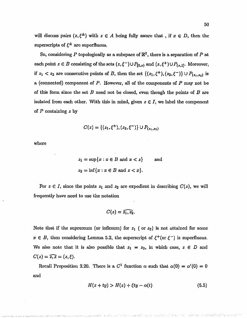
50
will discuss pairs ( z , ^ ) with z E A being fully aware that , if x E D, then the
superscripts of f are superfluous.
So, considering P topologically as a subspace of R2, there is a separation of P at
each point z E B consisting of the sets (2,£“ )UP[0,z) and (z ^ + JU P ^ ij . Moreover,
if z\ < Z2 are consecutive points of B, then the set {(21, £+ ), (22, ^- )} U P(2l,za) is
a (connected) component of P. However, all of the components of P may not be
of this form since the set B need not be closed, even though the points of B are
isolated from each other. With this in mind, given z E I, we label the component
of P containing 2 by
where
z\ = sup{x : x E B and x < 2} and
22 = inf{x : x E B and 2 < x}.
For 2 E / , since the points z\ and 22 are expedient in describing C(z), we will
frequently have need to use the notation
C(z) = 2TT*2-
Note that if the supremum (or infimum) for z\ ( or 22) is not attained for some
x E B, then considering Lemma 5.2, the superscript of £+(or £“ ) is superfluous.
We also note that it is also possible that z\ — 22, in which case, 2 E D and
C{z) = 2^2 = (2 ,0 -
Recall Proposition 2.20. There is a C 1 function a such that a(0) = a '(0) = 0
and
H(z + ty) > H(z) + ( ty - a(t) (5.5)

51
for each 0 < £ < 1, 2 € J, £ e dH(z), and y — ±1. For each (z ,£) 6 P define a
function g{•, 2, £) : R R by
g(x, 2, £) — H(z) + £(x - z ) - afla; - z\).
It is clear from (5.5) that g(x , 2, £) < H(x) for each x, with equality only at z — x.
Also, g(-, z , £) is C 1 for each (2, £) € P , and has derivative gx(x , 2 , £) = £—a'(|a:—2 |).
Moreover, #(•, •, •) and gx(-, •, •) are continuous as functions from I x P to R.
S tep I. For each z € I, we construct a special C l selection Sz(-) o fF on I such that
i f 2 ', 2" 6 C(z) — z u z i , then S z(x) = Sz>(x) for each x € I. In words, we construct
a selection unique to each component of P. Let S(x) be a fixed C 1 selection of F
on I (S will remain fixed henceforth). The selection S z(-) will have the following
properties:
(1) S'g(c) = H'+(c) and S z(d) = H'_(d), for each interval (c,d) of V with
Pc C C(z) (the intervals (c, d) refer to the disjoint intervals of V in the
representation 4.2).
(2) S z(x) > g{x,c,£+) and Sz(x) > g(x,d,£~) for each x e (c,d) for each
interval (c,d) o f V with P(c,d) C C(z).
(3) for each z € I, Sz (x) coincides with the fixed selection S(x) for each x £
(x \ ,X 2 ) where x i = sup{y : y 6 A and y < 21} and X2 = inf{y : y 6
A and y > 22}
(4) Let {a;n} and {zn} be sequences of points of I. I f x n -> x € / and zn ->
2 G D, then S'Zn (xn) -> Sz(x). Moreover, i f x = 2 , then SZn(xn) —> H'(x).
Let (c, d) be an interval of V (remember that intervals (c, d) refer to the disjoint
intervals of V in the repx-esentation 4.2). We first construct a special C 1 selection
‘S[c,d](') of F on [c, d). For x e [c, d] define
h(x) = max{S(x) ,g(x ,c ,^+) ,g (x ,d , ( - ) } .

Then h(x) < H(x) for each x € (c,d), h(c) =■ H(c), and h(d) — H{d). Moreover,
h(') is lower-C1 on [c, d] since it is the max of C 1 functions; in particular, dh{-) is
submonotone. Also, for x 6 [c, d] sufficiently near c, h(x) — max.{S(x),g(x, c ,f+ )}
since g(x,d,£~) < H(x) for all x d. Thus h'+(c) exists and, furthermore, h+(c) =
H ’+(c), since <7'(c, c ,f+ ) = f + = i7+(c). Similarly, h'_(d) = H!_(d). Keeping in mind
Remark 4.17, there is a C 1 selection •S,[c,rfj(*) of the multifunction F(x) = {y : h(x) <
V < •P’C®)} defined on [c,d]. Necessarily, S[C)d](c) = H'+(c) and <S'[C)dj(d) = H'_(d).A
It follows from the definition of h that, for each x G (c, d),
S[c,d](x) > <?(a;,c,£+ ) and S[c4](x) > g(x,d,C)>
Moreover, as in (4.16), we have the estimate
- 2(d - c) < S j ^ x ) < JVf A - 2(d - c) (5.6)
where, in this case,
N [c,d] = P+(x ) W x ) - h(x)) + p(x) sup {H'+{y)} + (1 - p { x ) ) sup {h'+(y)}!/€(c,d] !/e[c,d)
and similarly
M f a = 0 + ( x ) ( H ( x ) - h ( x ) ) + l 3 ( x ) in fAH'4-y)} + (1 - P(x)) inf {h'+(y)}.1 ‘ v e [c ,d ] T v e [c ,d ]
Let z G I. We now define a C 1 selection Sz(-) of F on the interval [21, 22] cor
responding to the component C(z) = z ^ z i . It is clear that there are no points of
B strictly between z\ and 22 (otherwise C{z) would not be connected). How
ever, points of D may abound there. Thus, if (c,d) is an interval of V with
z\ < c < d < 22, then <SjCjdj(c) = H'(c) and •S'[Ci<J](d) = H'(d), Consequently,
if (cj,di) and (cj,dj) are such intervals with d; = Cj, then the selections ,</.](•)

53
and 5'[ci ,<fi](*) combine to form a C 1 selection of F on the combined interval (c;, dj).
Moreover, the estimates (5.6) ensure that, if given a sequence of intervals of V (still
between z\ and z2), say {(c*, d»)}, the selections S'[c.i(f.](‘) combine to form a G1
selection of F on the set U i^i[ct> t]* So define
■ {
S r c d ] (® ) , if a; € [c, d) C [ 2 1 ,2 2 ] where (c,d) is an interval of V,S,(x) '
F(x), if x € [ 2 1 , 2 2 ] \ V .
Sz(') is then a C 1 selection of F defined on [21, 22] since x € A D (21, 22) implies
that x € D. Note that «S'(2i) = # + ( 21) and Sz(z2 ) =
The selection Sz(-) must now be extended to the entire interval I. There are two
possibilities for the nature of the points z\ and 22; they may be in B or D. If they
are in D, then ££(21) = H'(zi) = <S"(zi) and Sz(z2 ) = H'(z 2 ) = S'(z2). In this«KS,
case, Sz(') is easily extended to I using £>(•). However, 21 and 22 may not be in D.
Let xi = sup{y : y € A and y < z\] and X2 = inf{?/ : y E A and y > 22}.
Then 21,22 € B and x\ < z\ < 22 < x%. Choose C l selections Ti(>) and T2(*)
of F on the intervals (a;i,zi) and (22, 0:2) respectively such that T{(x 1) = S \ x 1),
Tl(x2) = S '(x2), T{(z 1) = H'+(z 1), and T2'( 22) = H L ( z 2 ) . Define
Sz(x) = <
Sz (x), if X e [21,22],
Ti(x), if® 6[® i,« i],
T2(x), if x e [22,0:2],
. S(x), if x G [0 , mi] U [a:2, 1].
Then Sz (-) is a C1 selection of F on I, Note that if 21 G D 01* 22 € JQ, then x\ = 21
or o:2 = 22 respectively. In that case, the selection Ti(-) or ^ (O is trivial and,, as
noted before, Sz(') is extended by using only 5(>). If 21 G B or z2 € B, then 0:1 < 21
or o:2 > 22 respectively and the selection Ti(-) or T2(-) is definitely not trivial.
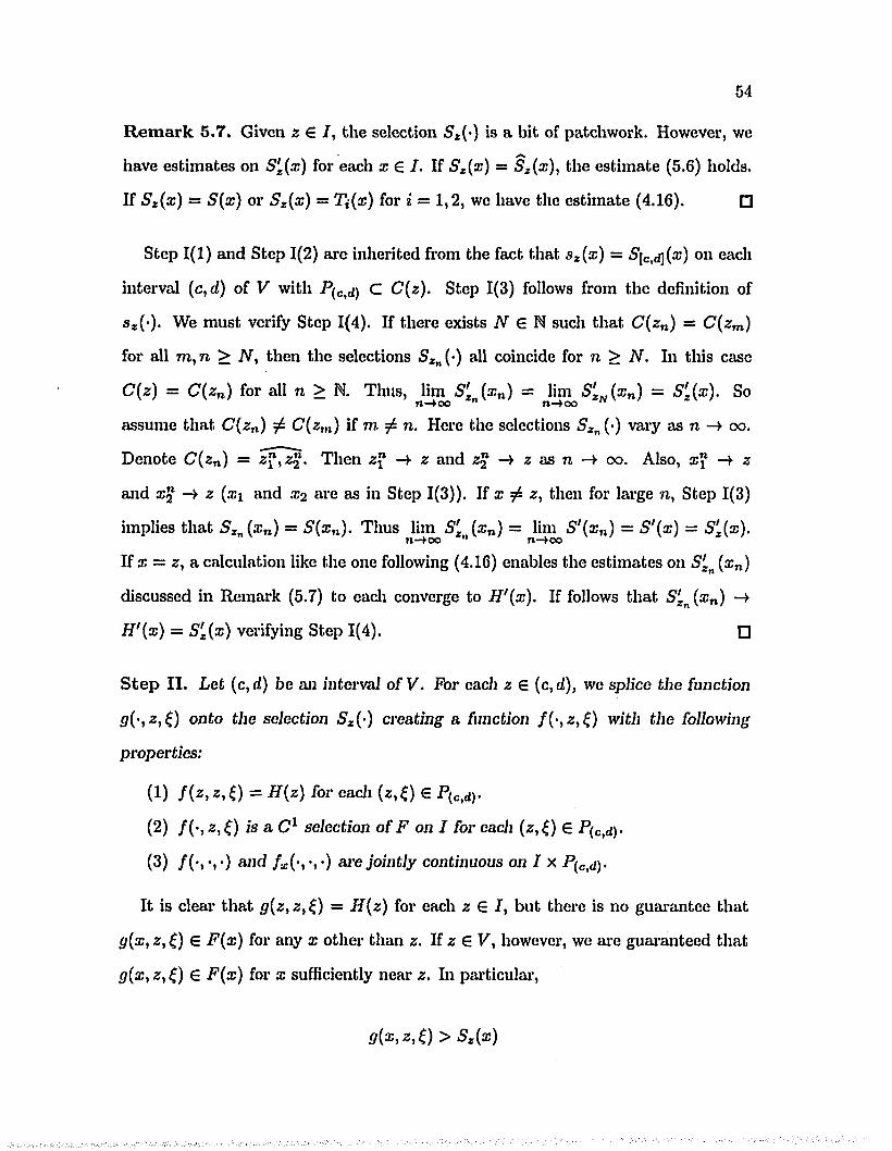
54
R em ark 5.7. Given z G J, the selection Sz{‘) is a bit of patchwork. However, we
have estimates on Sz(x) for each x G J. If Sz(x) = Sz(x), the estimate (5.6) holds.
If Sz(x) — S(x) or Sz(x) — Ti{x) for i — 1,2, we have the estimate (4.16). □
Step 1(1) and Step 1(2) are inherited from the fact that sz (x) = £[c,d](®) on each
interval (c,d) of V with P(c,d) C C(z). Step 1(3) follows from the definition of
sz(')- We must verify Step 1(4). If there exists N G N such that C(zn) = C(zm)
for all m ,n > JV, then the selections SZn (•) all coincide for n > N. In this case
C(z) = C(zn) for all n > N. Thus, lim SZn(xn) — lim S'ZN(xn) = S ^ x ) . So
assume that C(zn) ^ C(zm) if m ^ n . Here the selections SZn (•) vary as n —> oo.
Denote C(zn) = z^^z^. Then z™ —»■ z and z% z as n ► oo. Also, a:” —> z
and x% —► z (xi and X2 are as in Step 1(3)). If x ^ z, then for large n, Step 1(3)
implies that SZn(xn) = S(xn). Thus lim S'^fan) = lim S'(xn) = S'(x) — Sg(x).
If x = z, a calculation like the one following (4.16) enables the estimates on SZn (xn)
discussed in Remark (5.7) to each converge to H'(x). If follows that S'Zn (xn) ->
H'(x) = Sz{x) verifying Step 1(4). □
S tep II. Let (c, d) be an interval o fV . For each z G (c, d), we splice the function
g(-,z,£) onto the selection Sz (-) creating a function f( - ,z ,£) with the following
properties:
(1) /(*>*, 0 = H{z) for each (z ,() G P(c,d).
(2) f ( ' , z ,£ ) is a C l selection of F on I for each (z,£) G P(c,d)-
(3) /(•, •, •) and /*(•, •, •) are jointly continuous on I x P(c,d) •
It is clear that g{z,z, £) = H(z) for each z G J, but there is no guarantee that
g(x, z,£) € F(x) for any x other than z. If z G V, however, we axe guaranteed that
g(x, z,£) 6 F(x) for x sufficiently near z. In particular,
g ( x , z , £ ) > S z {x)

55
for x near z. Now fix an interval (c, d) of V and let Zq E ( c , d). The set P(c,d) i s
then entirely contained C ( z q ) — iTT^* Since the inequality in (5.5) is strict except
for t = 0, to each point (z,£) E P(c,d)> there correspond two points x~(z,£) and
:c+ (2,£) in (c,d) such that x~(z,$) < z < x+(z,£)> g(x-(z ,$) ,z ,$) = SZo(x-(z,$)),
g(x+(z,Z),z,Z) = SZo(x+(z,{)), and g(x,z,{) > S Zo(x) for all
x E 0e“ (2,£),:e+ (2,£)). In other words, x~(z,£) is the first point to the left of
z where <7(*, 2,£) is equal to the selection and a;+ (2,£) is the first point to
the right of z where <?(-,2, £) is equal to the selection S Zo(-). Moreover, The points
x^(z , £) vary continuously in (<?,£)•
We will now use Lemma 4.3 to splice each function g(',z,£) onto the selection
Smo (0 on the interval [a; (2 ,£),:c+ (2,£)] thereby keeping it in F and allowing it
to smoothly exit (c,d). Of course, the function v E C 1[a;-(z,£),a:+ (z,£)] created
by Lemma 4.3 will vary with the points x ± {z,£) so, for each (z,£) E P(c,d)> we
will be creating a C l function v(-,z,£). Remark 4.7 indicates that u (- ,v ) and
vx(', *, •) are jointly continuous on (c, d) x P(c,d)' Moreover, we will still require that
v(z ,z ,£) — H(z). To accomplish this, we alter <?(•, z,£) separately on each interval
[aT(2,f),2] and [«,®+(2,£)].
For each (z,£) € P{c,d)> and each x E I define
' « -(* ,« , 0» ® E [x-{z,£),z]
f ( x , z ,£ )= < v+(a: ,2 , f ) , x E [z,x+{z,£)\
, SZ0(x), ® g [ s “ (3,0>®+ (*»0]
where v+(x,z,£) is the function created on the interval [2 ,x + (2,£)] by Lemma 4.3
agreeing with g(‘,z ,£) and gx(',z ,£ ) at the point z and agreeing with <S'*0(-) and its
derivative at the point a;+ (2 ,£). The function v~(x, z, £) is its counterpart on the
interval [a?~(2 , f ) ,2]. So, for fixed (2 ,£) E P(c,d)> the function f ( ' , z ,£ ) is C l on I

and f(x,z,£) G F(x) for each x € I . M ore im portantly,
56
f ( x , x ^ ) - H { x ) . (5.6)
Also, /(•,•,*) and /*(•,•,•) are continuous on I x P(c,d)« Step 11(1), Step 11(2), and
Step 11(3) are satisfied. □
In this way, for each x G I and (z,£) G Py, the function f ( x , z, £) is defined.
For each (2 ,£) G Pa and x G / , define
f ( x , z ,£ ) = S z(x).
The function /(•, •, •) is now defined on all of I x P. However, many issues of its
continuity remain to be verified.
S tep II I . We verify that /(•,♦,•) and / x(-, •, •) are jointly continuous on I x P[Cidj
for each interval (c, d) of V.
Let (c, d) be an interval of V and z0 G (c, d). Then P(c,d) C C(z0) and we have
the selection Sm o( - ) corresponding to C ( z q ) . For each (2, £) G P(c,d) we have the
associated points ^ ( 2 , 0 as before. We first verify that /(•,•,•) and f x(•,•,•) are
jointly continuous on I x P(c,d]-.
Step 1(2) implies that
, = d ’ (5-8)
As a result, for each x ^ d, / ( x, z,£) = S , 0 (a) for all (2, £) G P(c,d) with 2 sufficiently
near d.
In order to show joint continuity, suppose (a:n, z n,£n) converges to (as,d, £~)
where each (xn,z n,{n) G I x P(c>d)- If x n £ (a_ (2n>£n),a+ (2n,£n)), then by defini
tion f ( x n, z nt£n) = 5Zo(a;n) for all n. So
lim f (xn,zn,^n) — lim SZQ(xn) — Sz0{x) — f{xtd,£ )n —too n —too

since S M is C 1. In this case, we are done. Assume x n G (x~(zni£n)iX+(zn,£n))
for each n. Then by (5.8), x = d. If x n — 2n, then f ( x n, z n,Zn) = H{xn) and
/*(z„, £„,£„) = Zn- Clearly then
hni /(a?n> zn> £n) — /(d , d, £ ).n —too
Moreover, by semismoothness and Step 1(1),
lim f z ( x n, z n,£n) = H'_(d) = S ' (d) = /* (d ,d ,f“ ).u —too w
So we are done in this case also.
Further assume that x n G (zn, x +(zn, f n))> the other case being similar. Then
/(®rn zni £n) = ujJ (xn, zn,Zn)-
To simplify notation in the following calculation, set x +(zn, £„) = x+ for each n G N.
By the Mean Value Theorems for derivatives and Clarke subgradients (Theorem
2.2) respectively , there exist points vn,wn G (xn,x+) and 7„ G dH(wn) such that
S'Z0M = and 7„ = ~ (5.9)-Zn X n X n — X n
Note that vn —> d and wn —> d. Let
N n = sup {max{gx(y, zn> {n)> SXQ (?/)}}.y6[*n ,1 1
Now by Step 1(1) and the continuity of S '0(-), S '0(d) = H'_{d), Also, gx(x, *„,£„) =
£n - a!{\x — zn\) with a'(-) continuous and a'(0) — 0, so that gx(d,d,£n) = H'_{d).

58
Employing the pointwise estimate discussed in Remark 4.7(2) and using (5.9),
we calculate
( v n )a: ix n> zni £ n ) ^ 9{x nt zni£n) SzpjXn) , N n2 “ x t - z n + 2
^ H (xn) - S ,0(xn) N n “ x t - Zn 2g(x„) - #(*+) f s ( x t ) - s » ( x t ) [ s , 0(x+) - Sa (xn)
Xn Zn Xn Zn Xn Zn
2~ ln ( x * — Xn) . H(x *) — Sg0(®£) . S'za{vn){x n ~ x n)
— Z I Z I---------------Z --------------------Xn Zn Xn Zn Xn — Zn
2— ( p t ( v \ \ (® n — ® «) . H{x n ) “ (x n ) . N n~ ( S * 0 (« » ) ~ 7 n ) — + — “ + -------- 1 + — + - r - .
***n "
Now, again by Step 1(1) and the continuity of 5 '0(-), lim S'Zo(vn) = S'ZQ(d) =vn
H'_{d). Moreover, since wn -> d and 7n 6 dH(wn), it follows from semismoothness
that lim 7n = H'_{d). Since the terms ~^~a!" are bounded between 0 and 1, wen —>00 *n z n
calculate
i>li,no ( (5 ;aK ) - 7„ ) < ^ l ) = 0 . (5.11)
We now turn our attention to the second term. Since g(x+,zn,€n) = SZo(x+) ^
follows that
S * o i x $ ) = + £ » ( * + - Zn) - a (® n “ z n)-
Subtracting H(x+) from each side and dividing by a;+ — zn
S Z0(x$) - H{x$) _ , a { x i - Zn) H (zn) - H(x+)— _ qn — | _ .Xn ~~ Zn Xn ' Zn Xn Zn
Taking limits above

59
lim S * o ( r t ) - H ( x + ) = R , __ H , ^ Qn - > o o X $ - Z n V '
since a/(0) = 0.
Using (5.10), (5.11), and (5.12) we take limits obtaining
lim v+(xn,z n,£n) < lim N n = H'_(d).n-¥oo n-*oo
This together with a similar lower estimate yields
(u+)x (xn, z n,£n) = H'_(d).
Then, by Step 1(1)
l i m f x (xn,z n^ n) = ^ l i m ^ + ^ Z n ,^ ) = H'_{d) = S'i0(d) = f x(d ,d ,C)-
We have verified that /(•, •, •) and f x(-, •, •) are jointly continuous on I x P{c,d\
If (x n , zn, £n) -)• (a;, c, £+ ), a similar examining of cases and taking of limits yields
lim f x(xn,zn,£n) = f x (x, c,£+).n—>oo
We have verified Step III. □
S tep IV . We verify that /(•, *, •) and f x(-, •, •) are jointly continuous on all of I x P.
Let (zo,*0,£o) 6 1 x P and (xn, z n,^n) -)• (a;o,*o,£o) where (xn,z ny£n) e l x P
for each n G N. It is clear that /(•, •, •) is jointly continuous on I x P. We must
show
lim f x(xni zn,£n) = / x{xq, zq,£q). (5.13)71 OO
Suppose zn e A for each n G N. Then zq G D s o that /(a:o,zo>£o) = ^ (rc o ).
Also, f ( x n, zn,£n) = S in (xn) since zn G A for each n G N. Thus, using Step 1(4),
lim f x (xn,z n, ( n) = lim S' (xn) = S'Zo(x0) = f x(xQ,z 0y^Q).n —too n —t oo ‘
In this case, (5.13) is verified.

60
Assume zn G V for each n G N. If Zq G V, (5.13) follows from Step II. So
assume Zo G A. If for large n, zn G (c, rf) where (c, d) is a fixed interval of V,
then Zo = c or zo — d and (5.13) follows from Step III. Suppose for large n that
zn G (Ci,di) U (cj, dj) where (cj, di) and (cj,dj) are fixed intervals of V such that
Ci = dj. We examine the case where Zq — a — dj (otherwise we are reduced to Step
III again). Denote those zn G (c;, di) by 2* and those zn G (Cj,dj) by z°n (assuming
that there are infinitely many points in each of the sequences, {z*J and {zfy, or
we are yet again reduced to Step III). If Zq G B, then ( z ^ Q ) -> (zo,H'_(zo)) and
(2n>£n) —> (zo,H'+(zo)). However, H'_{zq) < H'+(zq) contradicting the fact that
(xn, z n,£n) —> (xo,Zo,£o)- So Zq G D. Thus the intervals (c»,di) and (Cj,dj) are in
the same component, C(zq) of P. If xq ^ Zq, then for large enough n
f i ( ® m % n , £ n ) = ^ z 0 ( x n ) = 4 , ^ n )
from which (5.13) follows. Otherwise xo = z q . Then
l im /x (® n j £ n ) = f x { % 0) x 0) B ^ - ( x o ) ) = f x ( x 0i x 0> ■®-f(*Bo )) = f x { x m n —>oo
and (5.13) follows.
Finally, assume that for each n G N, zn G (ci(n),dqn)) for some interval
(cf(n),di(nj) of V. For convenience of notation, denote (cqn),di(n)) by (cn,dn).
Here the components C ^ n ) may vary with each n. Also, cn 20 and dn —> 20.
If xo zo, then Step 1(3) implies that f { x n,z n,£n) = S(xn) for all n large
enough. So (5.13) follows. Suppose xo = 20. The nature of f ( x n,z n,£n) de
pends upon the position of xn relative to zn. Recall that the function g(-,2n,£n)
was spliced onto the function S Zn{’) on an interval [x"(zn,£n),x+ (zn,£n)] to create
there. Otherwise, /(•, zn, £n) coincides with SZu (•), We first suppose
that x n $ [z~(2n,£n),x+ (2n,£n)] for each n G N. Then f ( x n,zn,£n) = SZn(xn)

61
and (5.13) follows from Step 1(4). Otherwise assume without loss of generality that
S ( ris (^ns £«))• Here /(S n )in i(n ) = ^n^tti^ni^n)* To show (5.13), it must
shown that
Jirn^ (w+)a (a:„, *„,£„) = H '(x0). (5.14)
The estimate and calculation required is identical to the one immediatly following
(5.10) except that the selections SZn (•) may vary in the present case. The conver
gence of that estimate was established by showing convergence of the terms (5.10),
(5.11), and (5.12). Now, the estimate for (5.10) becomes
N n = sup {max{<7x(7/, zn, fn), S'in (z/)}}.y€ [* n ,®n]
Considering Step 1(4), we have the same result as in (5.10). Step 1(4) also ensures
the same result as in (5.11). Finally, the right hand side of the estimate for (5.12) is
completely unaffected by any variation of the selection SZn('). So (5.12) also holds
in the present case. Thus, (5.14) is established. □
S tep V. We parametrize F with C 1 functions.
In similar fashion, we can construct a function / : I x Q —> K where Q is aA A
compact space and such that /(•, •, •) and f x(-, •, •) are jointly continuous on I x P .
Moreover,
h(x) = inf f (x ,q) .
Define the compact set S by
S = P x Q x [0,1].
Define p : I x S —> R by
p(x , s) = p(x,p, q, I) = l f (x ,p ) + (1 - l) f(x , q).
This is the desired parametrization of F. □

P roof o f Theorem 3.2 (necessity).
62
We offer the first part of this proof in higher dimensions to illustrate that the
Hamiltonian being jointly lower-C1 is a necessary condition in higher dimensions.
Again, let B n be the closed unit ball in Rn. Suppose that F : B n Rn is such that
F(x) = (p(a;,s) : s G 5} where p(-,s) is C 1 for each s G S, p (v ) and Vxp(*,*)
are jointly continuous, and S is compact. Now, for x G B n and p G Rn,
H(x,p) = sup (y,p)yGF(x)
= sup (p(x,s),p). s€S
Define / : R2n x S -4 R by /(x ,p , s) = {p(x,s),p). Then / is differentiable with
respect to (x ,p ). Moreover, /(-,-,•) and VX)P/(*, •, •) are continuous.
To show the second necessary condition, we revert to n = 1. Again, let H(x, 1) =
H(x) and h(x) = — H(x, — 1) for each x G [0,1], Suppose that H ( x q ) = h(xo). Let
Sx = {« G X : p(x , s) = H(x)}
and
S'x = {s G X : p(x , s) = h(x)}.
Clearly Smo = S ^ . Recall the representation (2.4). Then
dH(x0) = ca{px (x(hs) : s £
= co{pz(a;o,s) : s G S'Xo}
= dh(x o).

BIBLIOGRAPHY
[1] J.P.Aubin and H.Frankowska, Set-Valued Analysis, Birkhauser, 1990.
[2] C.Castaing, Sur les multi-application measurables, Inf. Rech. Op. 1 (1967), 91-126.
[3] C.Castaing and M.Valadier, Convex Analysis and Measurable Multifunctions, Springer-Verlag, Lecture Notes in Math 580.
[4] F.H. Clarke, Generalized gradients and applications, IVans. Am. Math. Soc. 205 (1975), 247-262.
[5] F.H. Clarke, Optimization and Nonsmooth Analysis, Wiley-Interscience, 1983.
[6] I.Ekeland and M.Valadier, Representation of set-valued mappings, J. Mat. Anal. Appl. 35 (1971), 621-629.
[7] G.Lebourg, Valeur moyenne pour gradient generalise, C.R. Acad. Sci. Paris Ser. A 281 (1975), 795-797.
[8] S.Lojasiewicz Jr., Some theorems of Scorza-Dragoni type for multifunctions with applications to the problem of existence of solutions for differential multivalued equations, Mathematical Control Theory (1985), 625-643.
[9] S.Lojasiewicz Jr., Parametrizations of convex sets (to appear), J. Approx. Theory.
[10] E.Michael, Continuous selections I, Annals of Math. 63 (1956), 361-381.
[11] R.Mifflin, Semismooth and scmiconvex functions in constrained optimization, SIAM J. Control Optimization 15 (1977), 959-972.
[12] A.Ornelas, Parametrization of Caratheodory Multifunctions, SISSA.
[13] R.Rockafellar, Lipschitzian properties of multifunctions, J. Nonlinear Anal. T.M.A. 9 (1985), 867-885.
[14] R.Rockafellar, Convex Analysis, Princeton University Press, Princeton NJ, 1970.
[15] R.Rockafellar, Favorable Classes of Lipschitz Continuous Functions in Subgradient Optimization, Progress in Nondifferentiable Optimization, Pergamon Press, New York, 1982.
[16] H.L.Royden, Real Analysis, 3rd ed., Macmillan, New York, 1988.
[17] J.E. Spingarn, Submonotone subdifferentials of Lipschitz functions, Trans. Am. Math. Soc. 264 (1981), 77-89.
[18] D.M. Wagner, Survey of measurable selection theorems, SIAM J. Control Optimization 15 (1977), 859-903.
63
VITA
The author, Craig Knuckles, was born the youngest of two children in Fort
Wayne, Indiana on April 19, 1967 to Mr. and Mrs. Otis Knuckles. He attended
High School at Heritage High School in Monroeville, Indiana and graduated in
1985. He received the Bachelor of Science degree in Mathematics at Tennessee
Technological University in 1989. He subsequently received the Master of Science
degree in Mathematics at Tennessee Technological University in 1991. He then
received a Board of Regents Fellowship at Louisiana State University where he
earned the Doctor of Philosophy degree in Mathematics in 1995. Craig was married
to Hope. E. Baskerville in 1992.
64

DOCTORAL EXAMINATION AND DISSERTATION REPORT
Candidate:
Major Field:
Title of Diaaertation:
Date of Examination:
Craig Knuckles
Mathematics
Continuously Differentiable Selections and Parametrizations of Multifunctions in One Dimension
Approved:
Major Profeaaor and Chairman
6£l the^Graduate School
E X A M IN IN G CO M M ITTEE:
March 31, 1995