Continuum Approach to Two- and Three-Phase Flow during Gas-Supersaturated Water Injection in Porous

Media

by

Robert Enouy

A thesis

presented to the University of Waterloo

in fulfillment of the

thesis requirement for the degree of

Master of Applied Science

in

Chemical Engineering

Waterloo, Ontario, Canada, 2010

©Robert Enouy 2010

ii

I hereby declare that I am the sole author of this thesis. This is a true copy of the thesis, including any

required final revisions, as accepted by my examiners.

I understand that my thesis may be made electronically available to the public.

iii

Abstract

Degassing and in situ formation of a mobile gas phase takes place when an aqueous phase equilibrated

with a gas at a pressure higher than the subsurface pressure is injected in water-saturated porous

media. This process, which has been termed supersaturated water injection (SWI), is a novel and

hitherto unexplored means of introducing a gas phase into the subsurface. Herein is a first macroscopic

account of the SWI process on the basis of continuum scale simulations and column experiments with

CO2 as the dissolved gas. A published empirical mass transfer correlation (Nambi and Powers, Water

Resour Res, 2003) is found to adequately describe the non-equilibrium transfer of CO2 between the

aqueous and gas phases. Remarkably, the dynamics of gas-water two-phase flow, observed in a series

of SWI experiments in homogeneous columns packed with silica sand or glass beads, are accurately

predicted by traditional two-phase flow theory which allows the corresponding gas phase relative

permeability to be determined. A key consequence of the finding, that the displacement of the aqueous

phase by gas is compact at the macroscopic scale, is consistent with pore scale simulations of repeated

mobilization, fragmentation and coalescence of large gas clusters (i.e., large ganglion dynamics) driven

entirely by mass transfer. The significance of this finding for the efficient delivery of a gas phase below

the water table in relation to the alternative process of in-situ air sparging and the potential advantages

of SWI are discussed.

SWI has been shown to mobilize a previously immobile oil phase in the subsurface of 3-phase systems

(oil, water and gas). A macroscopic account of the SWI process is given on the basis of continuum-scale

simulations and column experiments using CO2 as the dissolved gas and kerosene as the trapped oil

phase. Experimental observations show that the presence of oil ganglia in the subsurface alters gas

phase mobility from 2-phase predictions. A corresponding 3-phase gas relative permeability function is

determined, whereas a published 3-phase relative permeability correlation (Stone, Journal of Cana Petro

Tech, 1973) is found to be inadequate for describing oil phase flow during SWI. A function to predict oil

phase relative permeability is developed for use during SWI at high aqueous phase saturations with a

disconnected oil phase and quasi-disconnected gas phase. Remarkably, the dynamics of gas-water-oil 3-

phase flow, observed in a series of SWI experiments in homogeneous columns packed with silica sand or

glass beads, are accurately predicted by traditional continuum-scale flow theory. The developed

relative permeability function is compared to Stone’s Method and shown to approximate it in all regions

while accurately describing oil flow during SWI. A published validation of Stone’s Method (Fayers and

Matthews, Soc of Petro Eng Journal, 1984) is cited to validate this approximation of Stone’s Method.

iv

Acknowledgements

I am very appreciative of the guidance, extensive advice, encouragement, and support from my

supervisors, Dr. M. A. Ioannidis and Dr. A. J. Unger.

I would like to thank my lab mate Meichun Li for providing experimental data and advice leading to the

completion of this project.

I also appreciate the support from Ralph Dickhout, Ravindra Singh, Jeff Gostick, Lesley James, and

Dennis Herman.

v

Table of Contents

List of Figures .............................................................................................................................................. vii

List of Tables .............................................................................................................................................. viii

Nomenclature .............................................................................................................................................. ix

Chapter 1 ...................................................................................................................................................... 1

1. Introduction and Objectives ................................................................................................................. 1

1.1 Introduction .................................................................................................................................. 1

1.2 Project Objectives ......................................................................................................................... 3

Chapter 2 ...................................................................................................................................................... 4

2. Numerical Model .................................................................................................................................. 4

2.1 Theory ........................................................................................................................................... 4

2.2 Assumptions and Boundary Conditions ........................................................................................ 5

2.3 Formulation ................................................................................................................................... 7

Chapter 3 .................................................................................................................................................... 14

3. Gas Exsolution and Flow during Supersaturated Water Injection in Porous Media: ......................... 14

3.1 Experimental Methods and Supplemental Formulation ............................................................ 14

3.1.1 Experimental Methods ........................................................................................................ 14

3.1.2 Gas/Aqueous Phase Relative Permeability ......................................................................... 17

3.2 Results and Discussion ................................................................................................................ 18

3.2.1 SWI Transient and Steady State Behaviour......................................................................... 18

3.2.2 Post-SWI transient .............................................................................................................. 26

Chapter 4 .................................................................................................................................................... 31

4. Oil Recovery and Flow during Supersaturated Water Injection in Porous Media: ............................. 31

4.1 Experimental Methods and Supplemental Formulation ............................................................ 31

4.1.1 Experimental Methods ........................................................................................................ 32

4.1.2 Aqueous/Gas Phase Relative Permeability ......................................................................... 33

4.1.3 Oil Phase Relative Permeability Function ........................................................................... 35

4.2 Results and Discussion ................................................................................................................ 37

4.2.1 Short-term Experiments and Simulations ........................................................................... 37

4.2.2 Long-term Experiments and Simulations ............................................................................ 39

4.2.3 Enouy Approximation of Stone’s Method .......................................................................... 41

Chapter 5 .................................................................................................................................................... 47

vi

5. Conclusions ......................................................................................................................................... 47

5.1 Gas Exsolution and Flow during Supersaturated Water Injection in Porous Media ............... 47

5.2 Oil Recovery and Flow during Supersaturated Water Injection in Porous Media .................. 48

References .................................................................................................................................................. 49

vii

List of Figures Figure 1 – Boundary conditions for experiments 1-16. ................................................................................ 6

Figure 2 - J-function for air-water drainage in homogeneous packs of sand and glass beads. .................... 9

Figure 3 – Experimental setup. ................................................................................................................... 15

Figure 4 - Aqueous and gas phase relative permeability curves. ............................................................... 17

Figure 5: Aqueous and gas phase effluent data and injection pressure data. ........................................... 19

Figure 6: Aqueous phase effluent during gas saturation growth. .............................................................. 21

Figure 7: Simulation gas saturation and CO2 concentration during SWI. ................................................... 22

Figure 8: Simulation mass transfer rates during SWI. ................................................................................. 23

Figure 9: Experimental (symbols) and simulated (lines) results for experiment 6. .................................... 25

Figure 10: Observed aqueous phase effluent rates for the post-SWI transient ......................................... 26

Figure 11: Gas saturation increase during SWI as a function of supersaturation. ..................................... 28

Figure 12: Experimental setup. ................................................................................................................... 32

Figure 13: Aqueous and gas phase relative permeability curves. .............................................................. 34

Figure 14: Experiment 15 short-term gas and aqueous phase effluent curves. ......................................... 37

Figure 15: Experiment 15 short-term oil recovery experiment and simulation. ........................................ 38

Figure 16: Experiments 10-14 long-term oil recovery experiments and simulations. ................................ 40

Figure 17: Example of saturation distribution produced at end of SWI oil recovery [21]. ......................... 41

Figure 18: Stone’s Method for producing oil phase relative permeability in 3-phase systems. ................ 42

Figure 19: Enouy approximation of Stone’s Method for oil phase relative permeability in 3-phase

systems. ...................................................................................................................................................... 43

Figure 20: Difference between Enouy approximation and Stone’s Method for oil phase relative

permeability in 3-phase systems. ............................................................................................................... 44

viii

List of Tables

Table 1: Component and phase property data (at 20oC). .......................................................................... 11

Table 2: Simulation parameters and their origin. ....................................................................................... 13

Table 3: Properties of packed columns used in CO2-SWI experiments. ..................................................... 29

Table 4: Experimental control variables and measurements. .................................................................... 29

Table 5: Column-average gas phase saturation and associated inlet aqueous phase CO2-supersaturation.

.................................................................................................................................................................... 30

Table 6: Properties of packed columns SWI experiments. ......................................................................... 45

Table 7: Experimental observations. .......................................................................................................... 45

Table 8: Simulation results and parameters. .............................................................................................. 46

ix

Nomenclature [−] [dim] dimensionless

𝑝 components: water (𝑤), air (𝑎), oil (o) and carbon

dioxide (𝐶𝑂2)

𝑙 phases: aqueous (𝑞), non-aqueous (n) and gas (𝑔)

𝑆𝑙 [−] saturation of phase 𝑙

𝑃𝑙 [kPa] pressure of phase 𝑙

𝑀𝑙 [mole m3⁄ ] molar density of phase 𝑙

𝑋𝑝𝑙 [−] mole fraction of component 𝑝 in phase 𝑙

𝜌𝑙 [kg m3⁄ ] mass density of phase 𝑙

𝜇𝑙 [kPa ∙ day] viscosity of phase 𝑙

𝜙 [−] porosity of porous media

K [m2] Intrinsic permeability of porous media

𝑘𝑟𝑙 [−] relative permeability of phase 𝑙

𝐷𝑝𝑙 [m2 day⁄ ] molecular diffusivity of component 𝑝 in phase 𝑙

𝜏 [−] tortuosity of porous media

𝛼𝐿𝑙 [m ] longitudinal dispersivity of phase 𝑙

𝛼𝑇𝑙 [m ] transverse dispersivity of phase 𝑙

𝑄𝑝 [mole (m3 ∙ day)⁄ ] source (+ve) or sink (-ve) term for component 𝑝

𝐵𝑜 [−] Bond number

𝑔 [m/s2] gravitational acceleration

∆𝑆�̅� [−] change in column-averaged gas saturation

𝐽�𝑆𝑞� [−] Leverett J-function

𝑘𝑟𝑙

𝑘𝑟𝑛𝑐𝑞

𝑘𝑟𝑛𝑐

[−]

[−]

[−]

relative permeability of phase 𝑙

oil relative permeability at connate water

critical oil relative permeability

𝑛𝑙 [−] relative permeability exponent of phase 𝑙

𝑆𝑙𝑟 [−] irreducible saturation of phase 𝑙

𝑃𝑐𝑔𝑞 [kPa] capillary pressure between aqueous and gas

phases

𝒮𝑓 [−] super-saturation factor

x

∆𝒮𝑓 [−] change in super-saturation factor

𝑡0 [min] starting time of SWI experiment

𝑡𝑆𝑊𝐼 [min] end time of SWI experiment

𝑡𝓅−𝑆𝑊𝐼 [min] end time of post-SWI experiment

𝑄𝑔𝑒𝑓𝑓(𝑡) [mL/min] experimental gas phase effluent rate

𝑄𝑞𝑖𝑛𝑗(𝑡) [mL/min] experimental aqueous phase injection rate

𝑄𝑞𝑒𝑓𝑓(𝑡) [mL/min] experimental aqueous phase effluent rate

𝑋𝐶𝑂2 𝑞∗ [−] equilibrium CO2 mole fraction in aqueous phase

𝑋𝐶𝑂2 𝑞𝑖𝑛𝑗

Λ

[−]

[−]

injected aqueous phase CO2 mole fraction

gas phase effects on oil phase mobility multiplier

𝜎𝑝1,𝑝2 [N/m] surface tension between phases, p1 and p2

𝑑𝑝 [m] particle diameter of porous media

𝑆𝑔𝑛𝑢𝑐

𝑆𝑛𝑟𝑐

[−]

[−]

minimum gas saturation to initiate nucleation

Critical oil saturation during SWI

𝛽0, 𝛽1 ,𝛽2 𝑔, 𝛽2 𝑞 ,𝛽3 , 𝛽4 [−] non-equilibrium (kinetic) mass transfer coefficients

𝑃ref [kPa] reference pressure

𝑇ref [°K] reference temperature

𝑎𝑤𝑔𝑞 [kPa] equilibrium partitioning of water between gas and

aqueous phases

𝑎𝐶𝑂2 𝑔𝑞 [kPa] equilibrium partitioning of CO2 between gas and

aqueous phases

1

Chapter 1

1. Introduction and Objectives

1.1 Introduction

Gas saturation can develop in-situ within initially water-saturated porous media after the injection of an

aqueous phase that is equilibrated with gas at a pressure higher than the subsurface pressure. During

this process, hereafter referred to as supersaturated water injection (SWI), departure from

thermodynamic equilibrium (supersaturation of the aqueous phase) leads to the activation of nucleation

sites on the solid surface and the appearance of gas bubbles. Continual transport of solute from the

bulk aqueous phase to the gas-liquid interfaces leads to gas phase growth, which at the pore-scale leads

to the pressurization of bubbles confined in pores by capillary forces and their subsequent expansion

into adjacent water-filled pores. A ramified pattern of gas-occupied pores (gas clusters) develops under

the influence of capillarity and buoyancy. Gas cluster coalescence during growth, mobilization of

sufficiently large clusters under the action of buoyancy, and subsequent fragmentation resulting from

capillary instabilities also contribute to the complexity of this process, which was studied by pore

network simulation in the first part of this contribution [1]. The simulations suggest that a region of

finite extent, where gas exsolution takes place, is established with time in the vicinity of the injection

point. Mass transfer from the aqueous to the gas phase is confined in this region, the outer boundaries

of which are characterized by dissolved gas concentrations at near-equilibrium levels with the gas phase.

Continuous generation of gas within this region drives immiscible displacement and outward

propagation of the gas phase. Pore network simulations [1] indicate that advection of the gas phase

takes place via a repeated sequence of gas cluster mobilization, fragmentation and coalescence events

governed by the interplay of capillary and buoyancy forces. The two-phase flow regime established at

steady state is thus likely one of “large ganglion dynamics” rather than “connected pathway flow” [2, 3].

Interest in SWI is motivated by the need to improve the delivery of a gas phase to subsurface

environments contaminated by non-aqueous phase liquids (NAPL). Delivery of a gas phase below the

water table is needed in bioremediation applications, where oxygen or other reactive gases must be

supplied to sustain the destruction of dissolved organic contaminants by micro-organisms [4]. In other

instances where contaminants are present as NAPL ganglia trapped below the water table, volatilization

2

into a flowing gas phase may be an effective remedial strategy [5, 6]. To achieve these goals, in-situ air

sparging (IAS) has been used to date with varying success [7]. Mass transport effectiveness obviously

depends on the spatial distribution of air that can be achieved by IAS within a saturated aquifer. For this

reason, a large number of studies have sought to observe and explain the patterns of gas flow during gas

injection [8, 9, 10, 11, 12, 13, 14-17]. At the pore scale, variations in air entry pressure due to the

ubiquitous random disorder of the pore structure govern the migration of the injected air. During IAS,

buoyancy and a highly unfavorable viscosity ratio both have a destabilizing effect on the displacement

front which results in the migration of air away from the injection point in the form of separate

continuous channels. This picture cannot be accommodated by continuum models of multiphase flow

[8, 11, 14, 17] which are consequently limited in their ability to predict air sparging performance in

terms of mass transfer.

Bypassing of large portions of the target remediation area due to channeling of the injected air can

greatly compromise the remediation effectiveness of IAS. For SWI, on the other hand, one might expect

the gas saturation distribution to be relatively insensitive to random disorder of pore size and

permeability, at least within the region where gas exsolution takes place. Such an expectation arises

from the fact that nucleation can take place in pores of all sizes and the necessary condition for gas

cluster growth is transfer of solute mass from the flowing aqueous phase. Gas cluster growth is initially

more rapid in areas where the aqueous phase flow velocity is greater, i.e. in more permeable regions

within the porous medium. At the same time, an increase of the gas saturation causes reduction of the

effective permeability of these areas. Thus, a greater amount of the injected aqueous phase is diverted

to less permeable areas, where gas saturation can also develop, as long as the flowing aqueous phase

contains sufficient amount of dissolved gas for activation of nucleation sites and sustained mass

transfer. Beyond the region where gas exsolution takes place, increasing gas saturation occurs as a

result of immiscible displacement. At this scale, gas phase mobility is difficult to ascertain by pore

network modeling [1] and a macroscopic (continuum) description of SWI becomes necessary.

Recently, the SWI technology has been show to mobilize non-volatile NAPL ganglia trapped below the

water table [18]. Since the mobilization of oil in the subsurface is not clearly understood experiments

were conducted to characterize the mechanisms that make an otherwise immobile phase mobile.

Short-term and long-term experiments were conducted to determine the effects of three mobile phases

in unconsolidated porous media. Short-term experiments provide detailed data collection during the

development of gas saturation throughout the column and the resulting aqueous phase effluent. Long-

3

term experiments focus on the mobilization of oil and the overall oil recovery that can be achieved with

three mobile phases.

1.2 Project Objectives

The objective of this project is to measure the dynamics of gas exsolution and flow, as well as oil

recovery and flow, observed in long columns, packed with silica sand or glass beads under different

conditions (grain size, flow rate and dissolved gas concentration of the injected aqueous phase) of SWI

with CO2 as the dissolved gas. The experimental observations are interpreted using a multiphase,

compositional continuum model (CompFlow-SWI) based on the following hypotheses.

• The first hypothesis is that non-equilibrium mass transfer of CO2 between the aqueous and gas

phases can be described by the correlation of Nambi and Powers [19] modified to capture

nucleation within the context of continuum modeling. This hypothesis logically follows from

pore network simulation results [1].

• A second hypothesis is that gas advection is stabilized by mass transfer so that displacement of

the aqueous phase by gas is compact at the macroscopic scale and can, therefore, be described

by a continuum model using relative permeability concepts. Specifically, a test is conducted to

determine whether the model-predicted advection of the leading edge of the gas phase at a

critical saturation is consistent with experimental data.

• The third hypothesis is that the mobility of a disconnected oil phase in the form of ganglia can

be predicted using continuum-scale concepts such as relative permeability.

• A fourth hypothesis is that a more accurate oil phase relative permeability function than Stone’s

Method can be produced for predicting 3-phase systems.

Specifically, the effects of mobile aqueous and gas phases are determined on a previously non-mobile

oil phase trapped in the form of ganglia in unconsolidated porous media. SWI experiments aim to

understand how aqueous and gas phases interact when mobile and extend this understanding to an oil

phase. Initially, Stone’s Method was used to determine the oil phase relative permeability in 3-phase

systems. However, Stone’s Method was found to be inadequate and a new function was developed and

calibrated in order to predict oil mobility during SWI in 3-phase systems.

4

Chapter 2

2. Numerical Model

2.1 Theory

The derivation of the numerical model in this section is based on the idea of using a continuum-based

multi-phase compositional approach to describe two processes that are postulated to be central to the

description of SWI in porous media. The first process is non-equilibrium (kinetic) transfer of CO2

between the gas and aqueous phases. It should be noted that such an approach does not simulate the

genesis and fate of the gas phase at the pore scale in terms of individual bubbles or distinct clusters of

gas-occupied pores, but rather in terms of local gas saturation averaged over a macroscopic volume of

the medium containing a multitude of pores. On the basis of experimental data pertaining to the

dissolution of residual NAPL in granular media, Nambi and Powers [19] have developed a mass transfer

correlation that is valid over a broad range of non-wetting phase saturations. Pore network simulations

detailed in the first part of this work [1] suggest that the Nambi and Powers [19] correlation can also be

used to describe CO2 mass transfer between the gas and aqueous phases during SWI. However, this

mass transfer correlation does not describe the kinetics of the initial stages of gas phase nucleation [20].

An ad hoc modification to the mass transfer correlation is used to account for the rapid increase of gas

saturation during nucleation.

The second process involves gas-aqueous-oil 3-phase flow at the continuum scale, where sustained gas

flow occurs by mass transfer from an injected aqueous phase rather than direct gas injection. In the

context of a continuum-level description, it is hypothesized that gas phase mobility can be described in

terms of a saturation-dependent gas relative permeability function and that the multiphase extension of

Darcy’s law suffices to describe the advective gas flux. A well-known consequence of this hypothesis for

one-dimensional displacement in homogeneous porous media is advection of the gas phase as a “shock

front”, in which its rate of advection is controlled by its relative permeability at a characteristic value of

gas phase saturation (greater than the residual gas phase saturation) in a manner analogous to that

predicted by the Buckley-Leverett equation [2]. It is also hypothesized that disconnected oil ganglia can

be mobilized in porous media by introducing mobile gas and aqueous phases. Experimental evidence

suggests that during the “shock front” development, a measureable volume of oil is mobilized and

5

removed from the system. It is a key objective of this project to evaluate whether these hypotheses

conform to experimental observations.

2.2 Assumptions and Boundary Conditions

For the purpose of this thesis assumptions were introduced in order to reduce the complexity of

modeling the system.

• Viscosities are assumed to be temperature independent. This does not affect the model

predictions because experimental conditions are always around 298K despite vapourization

occurring inside of the column. Viscosity is somewhat temperature independent unless large

temperature swings are incurred, which makes this a valid assumption.

• Equilibrium partitioning is assumed for the components air, water and oil for aqueous, gas and

NAPL phases. Carbon dioxide is the only component that undergoes non-equilibrium

partitioning as described by Nambi and Powers (equation 6).

• Pore sizes throughout the column are assumed to be constant. The column is always packed

with media that is considered homogeneous, which simply means that the particle sizes are

bound within a tight tolerance. If homogeneneity was not assumed for the column a cross-

sectional distribution of pore sizes would have to be statistically created for each node, which

would only further complicate the process and not significantly change prediction results.

• One difficulty when dealing with gas flow through porous media is the concept of gas

compressibility. The model can account for compressibility, pressure and volume changes

during transient and steady-state periods. Gas saturations are solely volume-based and a

volumetric displacement of the aqueous phase is a sufficient measure during the transient

period. However, the pseudo steady-state assumption in the 2-phase experiments is a time

when, by definition, there can be no further gas accumulation in the column. Although excess

aqueous phase is not observed in the effluent, gas compressibility could allow for gas-density

changes throughout this steady-state period. A gas density change would not cause a problem

with column saturation, but it may impact gas phase relative permeability if severe enough. It is

assumed the gas-density does not change significantly enough to affect flow.

• Unlike the aqueous phase, there is no previous experimental information to characterize gas

phase relative permeability (𝑘𝑟𝑔) in a mass-transfer controlled system. Gas phase flow during

SWI was observed to be compact unlike similar experiments conducted with air sparging. Gas

phase flow during SWI is assumed to follow a Corey curve with an irreducible saturation (𝑆𝑔𝑟)

6

and a Corey constant (𝑛𝑔). With knowledge of all other component and phase properties in the

2-phase system, it is assumed a Corey curve can be fitted to produce a predictive model.

• The displayed experiments in Chapter 3 and Chapter 4 were chosen because they contain the

most relevant and representative data set. All information and figures are available for each

experiment for which data has been presented in Chapter 3 and Chapter 4.

The boundary conditions for the fit and predictions of Chapter 3 and Chapter 4 can be found in Figure 1.

Figure 1 – Boundary conditions for simulations 1-16.

Initial conditions for each column experiment include aqueous, gas and oil saturations and no flowing

phase with a hydrostatic pressure gradient. For the experiments contained in Chapter 3 the initial

conditions consist of a water-saturated column with no gas or oil phase present. Chapter 4 experiments

consist of water-flood residual initial oil saturation, as defined in tables therein, under water-wetted

conditions with no gas phase present.

7

2.3 Formulation

Formulation of the numerical model CompFlow-SWI largely follows that of Forsyth [21]. However, the

description of the numerical model is restricted to focus only on those processes relevant to simulating

the SWI experiments described here. Specifically, CompFlow-SWI is a continuum-scale multi-phase,

multi-component compositional model that considers three mobile phases - the aqueous (𝑞), non-

aqeuous (𝑛), and gas (𝑔) phases. The components considered are water (𝑤), air (𝑎), oil (𝑜), and carbon

dioxide (𝐶𝑂2). The conservation of moles of component 𝑝 can be written as follows. It is important to

note that the water and air relationships were combined due to the assumption of equilibrium

partitioning throughout the simulation. Each equation (1-4) comprises an accumulation term, a

component balance and a molecular diffusion term for each phase. Carbon dioxide also has a

generation term which is observed as the rate of non-equilibrium partitioning.

water: 𝑝 = {𝑤}

𝜕𝜕𝑡

� 𝜙𝑆𝑙𝑀𝑙𝑋𝑤𝑙

𝑙=𝑞,𝑔

= − � ∇ ∙ (𝑀𝑙𝑋𝑤𝑙V𝑙)

𝑙=𝑞,𝑔

+ � ∇ ∙ (𝜙𝑆𝑙D𝑤𝑙𝑀𝑙 ∇𝑋𝑤𝑙)

𝑙=𝑞,𝑔

+ 𝑄𝑤 (1)

air: 𝑝 = {𝑎}

𝜕𝜕𝑡�𝜙𝑆𝑔𝑀𝑔𝑋𝑎𝑔� = −∇ ∙ �𝑀𝑔𝑋𝑎𝑔V𝑔� + ∇ ∙ �𝜙𝑆𝑔D𝑎𝑔𝑀𝑔 ∇𝑋𝑎𝑔� + 𝑄𝑎 (2)

carbon dioxide: 𝑝 = {𝐶𝑂2}

𝜕𝜕𝑡�𝜙𝑆𝑞𝑀𝑞𝑋𝐶𝑂2 𝑞� = −∇ ∙ �𝑀𝑞𝑋𝐶𝑂2 𝑞V𝑞� + ∇ ∙ �𝜙𝑆𝑞D𝐶𝑂2 𝑞𝑀𝑞 ∇𝑋𝐶𝑂2 𝑞� + �̇�𝐶𝑂2 + 𝑄𝐶𝑂2

𝜕𝜕𝑡�𝜙𝑆𝑔𝑀𝑔𝑋𝐶𝑂2 𝑔� = −∇ ∙ �𝑀𝑔𝑋𝐶𝑂2 𝑔V𝑔� + ∇ ∙ �𝜙𝑆𝑔D𝐶𝑂2 𝑔𝑀𝑔 ∇𝑋𝐶𝑂2 𝑔� − �̇�𝐶𝑂2

(3)

oil: 𝑝 = {𝑜}

𝜕𝜕𝑡�𝜙[𝑆𝑞𝑀𝑞𝑋𝑜𝑞 + 𝑆𝑛𝑀𝑛� = −∇ ∙ �𝑀𝑞𝑋𝑜𝑞V𝑞� − ∇ ∙ (𝑀𝑛V𝑛) + ∇ ∙ �𝜙𝑆𝑞D𝑜𝑞𝑀𝑞 ∇𝑋𝑜𝑞�

(4)

where 𝑄𝑝 is the rate at which component 𝑝 is injected/removed (+ve/-ve). By including 𝑄𝑝 in equations

1-4 it is implied that distributed sources/sinks are possible; however, for the purpose of this study only

8

point source/sink were used and are defined by system boundary conditions. Property data for each

phase can be found in Table 1.

In Eq. (3), �̇�𝐶𝑂2 represents the non-equilibrium partitioning rate for the exsolution of carbon dioxide

from the aqueous to the gas phase, and is given by:

�̇�𝐶𝑂2 = 𝑆𝑞𝛽2,𝑞𝑀𝑞𝜅𝐶𝑂2 �𝑋𝐶𝑂2 𝑞

∗ − 𝑋𝐶𝑂2 𝑞� (5)

where 𝑋𝐶𝑂2 𝑞∗ is the mole fraction of carbon dioxide in the aqueous phase in equilibrium with the gas

phase. The rate coefficient 𝜅𝐶𝑂2 is adapted from Nambi and Powers [19] and Unger et al. [22] as

equation 6:

𝜅𝐶𝑂2 = 𝛽0 �max�𝑆𝑔, 𝑆𝑔𝑛𝑢𝑐��𝛽2,𝑔 �𝛽3 + 𝑅𝑞

𝛽1�𝜙𝛽4𝐷𝐶𝑂2 𝑞

𝑑𝑝2 (6)

The rate coefficient 𝜅𝐶𝑂2 is a dynamic mass transfer coefficient correlation that was developed and

verified in a controlled laboratory experiment. The experiment related the effects of pore size, pore

velocity, saturation, and other characteristics to the overall rate of mass transfer through statistical

methods described in Nambi and Powers [19]. Although this study determined NAPL dissolution rates

into an aqueous phase, it is a close analogy to the non-equilibrium mass transfer experienced during

exsolution of a supersaturated gas from an aqueous phase.

A gas saturation, 𝑆𝑔𝑛𝑢𝑐, is introduced ad hoc to prevent the computation of unrealistically small mass

transfer rates during the initial stages of gas phase formation when 𝑆𝑔 < 𝑆𝑔𝑛𝑢𝑐, 𝑅𝑞 = �𝑣𝑞�𝜌𝑞𝑑𝑝/𝜇𝑞 is the

aqueous phase Reynolds number, �𝑣𝑞� is the magnitude of the interstitial aqueous phase velocity and 𝜌𝑞

is the mass density of the aqueous phase. The various parameters entering Eq. (6) are summarized in

Table 2.

The Darcy flux of each phase 𝑙 is given by:

V𝑙 = −K ∙𝑘𝑟𝑙𝜇𝑙

∇(𝑃𝑙 + 𝜌𝑙𝑔𝑧) (7)

and the dispersion/diffusion tensors have the form:

𝜙𝑆𝑙D𝑙 = 𝛼𝑇𝑙 V𝑙I + �𝛼𝐿𝑙 − 𝛼𝑇𝑙 �V𝑙V𝑙V𝑙

+ 𝜙𝑆𝑙𝜏𝐷𝑝𝑙𝐈 (8)

The following constraints exist for some of the above variables:

9

𝑆𝑞 + 𝑆𝑔 + 𝑆𝑛 = 1

𝑋𝑤𝑞 + 𝑋𝐶𝑂2 𝑞 + 𝑋𝑜𝑞 = 1 and 𝑋𝑤𝑔 + 𝑋𝑎𝑔 + 𝑋𝐶𝑂2 𝑔 = 1

𝑃𝑔 = 𝑃𝑛 − 𝛼𝑃𝑐𝑔𝑛�𝑆𝑔� + (1 − 𝛼)[𝑃𝑐𝑔𝑞�𝑆𝑔� − 𝑃𝑐𝑛𝑞(𝑆𝑞 = 1)]

𝑃𝑛 = 𝑃𝑞 + 𝛼𝑃𝑐𝑛𝑞�𝑆𝑞� + (1 − 𝛼)𝑃𝑐𝑛𝑞(𝑆𝑞 = 1)

𝛼 = min (1, 𝑆𝑛 𝑆𝑛∗⁄ )

(9)

(9a)

(9b)

(9c)

(9d)

where 𝑃𝑐𝑔𝑞 is the capillary pressure between the gas and aqueous phases; 𝑃𝑐𝑛𝑞 is the capillary pressure

between the water and oil phases; and 𝑃𝑐𝑔𝑛 is the capillary pressure between the gas and oil phases.

The relationships from equations 9-9d are delineated in Forsythe [18] where experimental justification is

provided. In essence, the available 2-phase capillary pressure data were combined using saturation

information as well as constant multipliers in order to produce 3-phase capillary pressure curves.

Aqueous-gas phase capillary pressure data, 𝑃𝑐𝑔𝑞, which for drainage in unconsolidated packs of glass

beads and silica sand were taken from the experimental studies of Ioannidis et al. [12] and Leverett [23]

respectively, and are plotted in Figure 2 in terms of the Leverett J-function 𝐽�𝑆𝑞�: note that each

capillary pressure is dependent on its corresponding saturation.

Figure 2 - J-function for air-water drainage in homogeneous packs of sand and glass beads.

0 0.1 0.2 0.3 0.4 0.5 0.6 0.7 0.8 0.9 10

0.5

1

1.5

2

2.5

Aqueous Phase Saturation

J-Fu

nctio

n

SandGlass Beads

10

𝐽�𝑆𝑞� =𝑃𝑐𝑔𝑞 �

𝑲𝜙�

0.5

𝜎𝑔𝑞 (10)

The Leverett J-function is a dimensionless function of water saturation describing a capillary pressure

curve [23]. The interfacial tensions were taken to be 26×10-3, 48×10-3 and 72×10-3 N/m2 for gas-oil, oil-

water and gas-water interfaces respectively. Porosity, absolute permeability, capillary pressure and

interfacial surface tensions can be determined from the column setup or independent of experiment.

Equilibrium partitioning of components between the aqueous and gas phases occurs according to the

following relationships:

𝑋𝑤𝑔 =𝑎𝑤𝑔𝑞𝑃𝑔

𝑋𝑤𝑞

𝑋𝐶𝑂2 𝑔 =𝑎𝐶𝑂2 𝑔𝑞

𝑃𝑔𝑋𝐶𝑂2 𝑞∗

(11)

With the air component being insoluble in water, 𝑋𝑎𝑞 = 0. This assumption follows from [21] and

allows the gas phase to be present to at least some minimal saturation 𝑆𝑔𝑚𝑖𝑛 = 10−3 ≪ 𝑆𝑔𝑛𝑢𝑐 , to

alleviate numerical issues associated with the non-condensable air component. Phase and component

properties pertinent to the experiments described in this work are listed in Table 2. On the basis of

literature values [20], a longitudinal dispersivity 𝛼𝐿𝑞= 0.1 m was considered representative of all packs in

this work with 𝛼𝑇𝑞 = 𝛼𝐿

𝑔 = 𝛼𝑇𝑔 = 0 .

Time derivatives in Eqs. (1-4) are discretized using finite differences with fully-implicit time weighting. A

finite volume discretization in one-, two- or three-dimensions is used to handle the spatial derivatives.

Details of the discretization can be found elsewhere [18, 21] and will not be repeated here. All of the

component equations are fully-coupled and full Newton-Raphson iteration is used for linearization. This

yields a large sparse Jacobian matrix which is subsequently solved using ILU factorization and either

CGSTAB or GMRES acceleration [24, 25, 26].

11

Table 1: Component and phase property data (at 20oC).

Property Value Source

Compressibility

�̂�𝑞 [kPa−1] 3.0×10-6 [27]

Standard component densities

𝑀𝑤∗ [mole m3⁄ ] 5.5×104 [27]

𝑀𝑎∗ [mole m3⁄ ] 41.1 [27]

𝑀𝐶𝑂2∗ [mole m3⁄ ]

𝑀𝑜∗ [mole m3⁄ ]

41.1

5.13×103

[27]

[27]

Molecular weights

𝜔𝑤 [kg mole⁄ ] 18.02×10-3 [28]

𝜔𝑎 [kg mole⁄ ] 28.97×10-3 [28]

𝜔𝐶𝑂2 [kg mole⁄ ]

𝜔𝑜 [kg mole⁄ ]

16.0×10-3

156.0×10-3

[28]

[28]

Reference pressure and temperature

𝑃ref [kPa] 100.0

𝑇ref [°K] 298.0

Viscosities

𝜇𝑞 [kPa ∙ day] 2.44×10-11 [28]

𝜇𝑔 [kPa ∙ day]

𝜇𝑛 [kPa ∙ day]

1.62×10-13

2.64×10-11

[28]

[28]

Molecular diffusion coefficient

𝐷𝑤𝑞 = 𝐷𝐶𝑂2𝑞 [m2 day⁄ ] 3.14×10-6 [29]

𝐷𝑤𝑔 = 𝐷𝑎𝑔 = 𝐷𝐶𝑂2𝑔 [m2 day⁄ ] 1.70×10-6 [29]

Molar density

𝑀𝑞 =

1 + �̂�𝑞�𝑃𝑞 − 𝑃ref�∑ max�0,𝑋𝑝𝑞�𝑝 𝑀𝑝

∗� , 𝑀𝑔 =

𝑃𝑔𝑅𝑇

12

Table 1 – Continued

Property Value Source

Mass density

𝜌𝑙 = �𝑋𝑝𝑙𝜔𝑝𝑝

Equilibrium partitioning coefficients

𝑎𝑤𝑔𝑞 [kPa] 11.96 [30]

𝑎𝐶𝑂2 𝑔𝑞 [kPa]

𝑎𝑜𝑛𝑔 [kPa]

1.651x105

0

[30]

Assumption

Interfacial tensions

𝜎𝑔𝑞 [N/m] 72×10-3 [30]

𝜎𝑛𝑞 [N/m]

𝜎𝑔𝑛 [N/m]

48×10-3

26×10-3

[30]

[30]

13

Table 2: Simulation parameters and their origin.

Property Value Source

Aqueous phase relative permeability in sand

𝑆𝑞𝑟 [−]

𝑛𝑞 [−]

Aqueous phase relative permeability in glass beads

𝑆𝑞𝑟 [−]

𝑛𝑞 [−]

2- phase gas relative permeability in sand and glass beads

𝑆𝑔𝑟 [−]

𝑛𝑔 [−]

3-phase gas relative permeability in sand and glass beads

𝑆𝑔𝑟 [−]

𝑛𝑔 [−]

3-phase oil relative permeability in sand and glass beads

𝑆𝑛𝑟𝑐 [−]

𝑛𝑛 [−]

Mass transfer rate parameters

𝑆𝑔𝑛𝑢𝑐 [−]

𝛽0 [−]

𝛽1 [−]

𝛽2 𝑔 [−]

𝛽2 𝑞 [−]

𝛽3 [−]

𝛽4 [−]

0.085

2.21

0.20

2.89

0.12

1.50

0.18

1.50

0.06

1.50

0.03

37.2

0.61

1.24

0.00

0.01

1.00

[23]

[23]

[12]

[12]

this study

this study

this study

this study

this study

this study

this study

[19]

[19]

[19]

[19]

[22]

[19]

14

Chapter 3

3. Gas Exsolution and Flow during Supersaturated Water

Injection in Porous Media:

Column Experiments and Continuum Modeling

3.1 Experimental Methods and Supplemental Formulation

3.1.1 Experimental Methods

A series of laboratory experiments was conducted in which an aqueous phase supersaturated with CO2

was injected at the bottom of a vertically-oriented packed column that was initially saturated with

degassed water. The solution is supersaturated in the sense that the concentration of CO2 in the

injected aqueous phase is greater than its solubility in water at the column pressure. In order to achieve

a supersaturated aqueous phase, tap water and CO2 gas from a pressurized cylinder were continuously

supplied to a hollow-fiber membrane contactor (InVentures Technologies), operating at a pressure of ca.

5 atm. The membrane contactor operates by maximizing the exposed surface area of aqueous phase to

a dissolvable gas phase at a calibrated pressure. The gas phase pressure is set slightly higher than the

liquid phase pressure and this condition is maintained with a controller. The gas phase pushes into the

hollow fibers creating a large gas-liquid interfacial surface area which allows for gas to more rapidly

dissolve into the aqueous phase.

Figure 3 depicts the experimental setup. A known volume of degassed water was initially added to a

Plexiglas column, which is 155 cm long and has an internal diameter of 76 mm. Enough space was

allowed for solid silica sand or glass beads to be subsequently packed. Solids were continuously added

and wet-packed under vibration or mechanical mixing to prevent the trapping of gas bubbles and to

reduce the possibility of layering. Some layering was occasionally observed during this. To prevent the

loss of solid particles, fine screens were placed at the top and bottom of the column and supported by

springs as necessary.

15

Figure 3 – Experimental setup.

Plates were bolted to the top and bottom of the column to create a closed system with an injection port

at the base and sampling ports over the length and at the top of the column. The porosity of the

packing was determined from knowledge of the column dimensions, mass of solids added, and the

volume of water displaced by the solids added. Finally, the absolute permeability of the packing was

determined by measuring the water flow rate under a fixed pressure gradient. Table 1 summarizes the

porous media properties for nine experiments forming the basis of this work. The ratio of buoyant to

capillary forces in these systems is also quantified in Table 1 in terms of the Bond number, defined as

follows:

𝐵𝑜 =�𝜌𝑞 − 𝜌𝑔� 𝑔 𝚱

𝜎𝑔𝑞 (12)

where 𝜌𝑞 and 𝜌𝑔 are the mass density of the aqueous and gas phases, 𝑔 is gravitational acceleration, 𝚱

is the absolute permeability of the system, and 𝜎𝑔𝑞 is the interfacial tension between the gas and

aqueous phases.

Aqueous and gas phase effluents from the column were sent to a graduated pipette acting as a phase

separator. The mass of aqueous phase effluent was collected in a beaker and measured continuously

using a digital balance interfaced with a computer. Also interfaced with a computer were a mass flow

meter (Omega, model FMA3304) to measure the effluent rate of gas consisting of nearly 100% CO2, and

a pressure transducer (Validyne, model DP10-44) to monitor the aqueous phase pressure at the base of

16

the column. Aqueous phase samples were drawn from sampling ports at distances of 75 cm and 145 cm

from the column base to determine the concentration of dissolved CO2.

At the start of each experiment the column was either freshly packed and, therefore, completely

saturated with degassed water, or flushed with copious amounts of degassed water to ensure that no

gas phase from a previous experiment remained entrapped in the porous media. To conduct an

experiment, the valve at the bottom was opened at time 𝑡0 and CO2‒supersaturated water was allowed

to flow through the column at constant rate until time 𝑡𝑆𝑊𝐼, a period of time sufficiently long for the

aqueous phase effluent rate to reach a constant steady-state value. At steady-state, the rate of

accumulation of gas within the column was zero and a measurement of the aqueous phase effluent rate

provided the flow rate of the injected aqueous phase, 𝑄𝑞𝑖𝑛𝑗. The mole fraction of dissolved CO2 in the

injected aqueous phase, 𝑋𝐶𝑂2 𝑞𝑖𝑛𝑗 , was also determined experimentally as follows because of the inability

to precisely control the level of super-saturation entering the system. Despite setting the pressure and

flow rates, the saturation unit was not able to produce predictable results. Once an experiment began,

the exsolution of carbon dioxide was able to create a consistent gas flow rate but that flow rate could

not be determined a priori.

Aqueous phase effluent was first drawn from the top sampling port following establishment of a steady

aqueous effluent rate. The effluent sample was immediately added to a sodium hydroxide solution of

pH greater than 11. The sodium hydroxide was in excess to ensure that all dissolved CO2 was converted

into disodium carbonate. This mixture was then titrated with hydrochloric acid using phenolphthalein as

the titration indicator. Initially the solution was translucent, but changed color as the pH was reduced to

11. The titration was complete when the pH dropped below 9 and the solution became translucent

once again. At this point, all of the disodium carbonate was converted into sodium bicarbonate and a

mole balance was used to determine the original amount and, hence, the mole fraction of CO2 in the

aqueous effluent. The mole fraction of carbon dioxide in the injected aqueous phase, 𝑋𝐶𝑂2 𝑞𝑖𝑛𝑗 , was then

determined from a steady-state mass balance of CO2 over the entire column using the experimentally

measured aqueous and gas phase effluent rates, 𝑄𝑞𝑒𝑓𝑓 and 𝑄𝑔

𝑒𝑓𝑓. The values of 𝑄𝑞𝑖𝑛𝑗 and 𝑋𝐶𝑂2 𝑞

𝑖𝑛𝑗 for

each experiment were determined from steady-state values of 𝑄𝑞𝑒𝑓𝑓 and 𝑄𝑔

𝑒𝑓𝑓 are listed in Table 4.

In each experiment, SWI was stopped at time 𝑡𝑆𝑊𝐼 and the column response was monitored over time

until steady-state was again reached. Experimental data from the two transient periods, one following

SWI commencement and the other following SWI termination, are particularly interesting because they

17

are sensitive indicators of the ability of the continuum model to describe the SWI process. In

subsequent sections, these data are discussed separately.

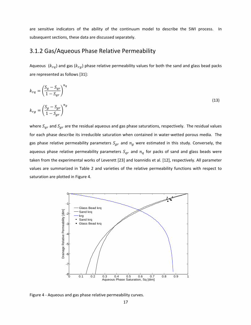
3.1.2 Gas/Aqueous Phase Relative Permeability

Aqueous (𝑘𝑟𝑞) and gas (𝑘𝑟𝑔) phase relative permeability values for both the sand and glass bead packs

are represented as follows [31]:

𝑘𝑟𝑞 = �𝑆𝑞 − 𝑆𝑞𝑟1 − 𝑆𝑞𝑟

�𝑛𝑞

𝑘𝑟𝑔 = �𝑆𝑔 − 𝑆𝑔𝑟1 − 𝑆𝑔𝑟

�𝑛𝑔

(13)

where 𝑆𝑞𝑟 and 𝑆𝑔𝑟 are the residual aqueous and gas phase saturations, respectively. The residual values

for each phase describe its irreducible saturation when contained in water-wetted porous media. The

gas phase relative permeability parameters 𝑆𝑔𝑟 and 𝑛𝑔 were estimated in this study. Conversely, the

aqueous phase relative permeability parameters 𝑆𝑞𝑟 and 𝑛𝑞 for packs of sand and glass beads were

taken from the experimental works of Leverett [23] and Ioannidis et al. [12], respectively. All parameter

values are summarized in Table 2 and varieties of the relative permeability functions with respect to

saturation are plotted in Figure 4.

Figure 4 - Aqueous and gas phase relative permeability curves.

0 0.1 0.2 0.3 0.4 0.5 0.6 0.7 0.8 0.9 1-8

-7

-6

-5

-4

-3

-2

-1

0

Aqueous Phase Saturation, Sq [dim]

Dra

inag

e R

elat

ive

Perm

eabi

lity

[dim

]

Glass Bead krqSand krqkrgSand krqGlass Bead krq

18

The shaded symbols shown in Figure 4 are the experimental steady state aqueous phase relative

permeability values for glass bead (circles) and sand pack (triangles) were computed by using the multi-

phase extension of the Darcy equation as: 𝑘𝑟𝑞�𝑆𝑞� = �𝑄𝑞𝑖𝑛𝑗 𝜇𝑞 𝐿� �𝐊 𝐴 𝛥𝛤𝑞�� where 𝐿 is the column

length, 𝐴 is its cross-sectional area, 𝛥𝛤𝑞 = 𝑃𝑞(𝑡𝑆𝑊𝐼) − 𝑃ref − 𝜌𝑞𝑔𝐿 , and 𝑆𝑞 = 1 − ∆𝑆�̅�(𝑡𝑆𝑊𝐼). It should

be noted that actual experimental data was used to find these data points. The points are plotted to

reaffirm that the Leverett and Ioannidis relative permeability curves are valid during experiment.

Since the gas phase relative permeability has never been measured for flowing gas exsolution in the

presence of a flowing aqueous phase, it had to be estimated. The gas phase relative permeability curve

was assumed to have the shape of a Corey curve with irreducible gas saturation and a Corey constant.

To estimate these values, experiments 1-8 were simulated with a trial and error method. The

irreducible saturation and the Corey constant appear to be heavily correlated and only one combination

of the two were able to reproduce each experiment. The simulation results are highly sensitive to any

change in the irreducible saturation and the Corey constant.

3.2 Results and Discussion

In the simulations reported here, only 𝑆𝑔𝑛𝑢𝑐 (see Eq. (6)) and the gas relative permeability parameters

𝑆𝑔𝑟 and 𝑛𝑔 (see Eq. (13)) were considered adjustable. Every other parameter was independently

measured or estimated: such as absolute permeability, injection pressure, aqueous phase carbon

dioxide content, aqueous phase flow rates, aqueous phase relative permeability curves, and mass

transfer interactions. Experimental observations and numerical results are discussed which pertain to

the time period 𝑡0 ≤ 𝑡 ≤ 𝑡𝑆𝑊𝐼 (SWI transient and steady state) from those pertaining to the time period

𝑡𝑆𝑊𝐼 < 𝑡 ≤ 𝑡𝓅−𝑆𝑊𝐼 (post-SWI transient), all with reference to experiment 8 (see Tables 3 and 4) against

which the continuum model is calibrated. Subsequently, it is hypothesized that the remaining

experiments can be predicted using the same set of parameter values ( 𝑆𝑔𝑛𝑢𝑐, 𝑆𝑔𝑟 , 𝑛𝑔). The post-SWI

information affords an additional test on the ability of the continuum model to describe gas exsolution

and flow when SWI is stopped, but a driving force for mass transfer remains. This driving force is a

consequence of two factors, volumetric expansion of the gas phase as pressures return to hydrostatic

and an increase in the level of CO2 supersaturation of the aqueous phase due to the decline in aqueous

phase pressure.

3.2.1 SWI Transient and Steady State Behaviour

19

Figure 5 shows the experimental (symbols) and simulated (lines) results for experiment 8. The black

circle denotes the pore volume relative time that the aqueous phase effluent sample was taken and

used to determine 𝑋𝐶𝑂2 𝑞𝑖𝑛𝑗 as listed on Table 3.

The aqueous phase effluent increases very rapidly above the expected 𝑄𝑞𝑖𝑛𝑗, during the early time

periods where no gas phase effluent is produced. A rapid increase of the injection pressure is also

observed as the relative permeability of the aqueous phase is reduced in the presence of gas within the

pore space. As soon as SWI is initiated, miscible displacement of the CO2-free resident aqueous phase

by the CO2-rich injected aqueous phase takes place, resulting in nucleation and growth of the gas phase

in the lowest part of the column.

Figure 5: Aqueous and gas phase effluent data and injection pressure data.

As gas saturation develops, a volumetric displacement occurs which is observed as an increase in the

aqueous phase effluent rate. The aqueous phase injection rate, 𝑄𝑞𝑖𝑛𝑗, is constant throughout the

experiment, which allows for the aqueous phase effluent rate, 𝑄𝑞𝑒𝑓𝑓, to be used as the primary method

to calculate the average gas saturation in the column. The total volume of displaced aqueous phase and

thus the column-averaged change in gas saturation ∆𝑆�̅� at time 𝑡𝑆𝑊𝐼 can be determined as follows:

0 1 2 3 4 5 6 7-10

0

10

20

30

40

50

60

Gas Phase Effluent

Aqueous Phase Effluent

Injection Pressure

Pore Volumes Injected

Flow

Rat

e (m

L/m

in)

0 1 2 3 4 5 6 70

50

100

150

200

250

300

350

Inje

ctio

n Pr

essu

re (k

Pa)

qQeff

20

∆𝑆�̅�(𝑡𝑆𝑊𝐼) ≈ � [𝑄𝑞𝑒𝑓𝑓(𝑡) − 𝑄𝑞

𝑖𝑛𝑗] 𝑑𝑡

𝑡𝑆𝑊𝐼

𝑡0

(14)

At the end of the transient period, 𝑄𝑞𝑒𝑓𝑓 = 𝑄𝑞

𝑖𝑛𝑗, and the rate of gas accumulation in the column is zero.

It is important to note that gas flow out of the column does not begin until the gas saturation is nearly

fully developed. The aqueous phase effluent rate, 𝑄𝑞𝑒𝑓𝑓, remains constant thereafter until SWI is

terminated at time 𝑡𝑆𝑊𝐼, after injection of about 6 PV of CO2-supersaturated aqueous phase. On the

contrary, the measured gas flow rate which reaches a maximum once a steady gas saturation is

established, is observed to decrease gradually with time as a result of a decreasing mole fraction of

dissolved CO2 in the injected aqueous phase, 𝑋𝐶𝑂2 𝑞𝑖𝑛𝑗 . This is a consequence of unpredictable variability in

the performance of the membrane contactor.

No attempt was made to incorporate temporal changes of 𝑋𝐶𝑂2 𝑞𝑖𝑛𝑗 in the simulation. Instead, it was

assumed that 𝑋𝐶𝑂2 𝑞𝑖𝑛𝑗 is constant and equal to the value determined experimentally as explained in

Section 3.1.1. The actual aqueous phase sample used to perform this calculation is shown by the large

open circle in Figure 5. The simulation accurately reproduces experimental measurements of aqueous

phase effluent flow, gas phase effluent flow, and injection pressure throughout the time period

𝑡0 ≤ 𝑡 ≤ 𝑡𝑆𝑊𝐼. Such agreement was achieved using the gas phase relative permeability function plotted

in Figure 3 and 𝑆𝑔𝑛𝑢𝑐 = 0.03 in the mass transfer rate expression, Eq. (6). It was found that unless such

an ad hoc modification of the mass transfer rate expression is made, the continuum model is unable to

accurately describe the dynamics of gas accumulation in the column for any choice of gas phase relative

permeability. This is to be expected because the kinetics of the initial stages of gas phase formation

(nucleation) [20, 32], which are not explicitly accounted for in the continuum model, are markedly

different from the kinetics of non-equilibrium mass transfer between a flowing aqueous phase and non-

wetting gas phase ganglia [19].

A more in-depth examination of the experimental observations is possible with the help of the

numerical model. Figure 6 shows again measured and predicted aqueous phase effluent during the

initial transient period of SWI.

21

Figure 6: Aqueous phase effluent during gas saturation growth.

The experimental (symbols) and simulated (line) aqueous phase effluent rate during SWI as a function of

PV of aqueous phase injected (experiment #8): A = 0.10 PV, I = 0.34 PV and J = 0.36 PV. A number of

time points of interest to this transient behavior are identified with letters (A, I, and J) in this figure.

These points are discussed with reference to Figure 7, which plots the simulated spatiotemporal

evolution of gas phase saturation and CO2 content of the resident aqueous phase. Figure 6 also presents

the mole fraction of dissolved CO2 at conditions of equilibrium between the gas and aqueous phases,

determined from Henry’s law (see Eq. (10)) at the prevailing steady-state aqueous phase pressure

distribution and temperature 𝑻𝐫𝐞𝐟.

0 0.1 0.2 0.3 0.4 0.5 0.625

30

35

40

45

50

Pore Volume

W a t e r E f f l u e n t , Q q [ m L / m i n ]

AI

JK

22

Figure 7: Simulation gas saturation and CO2 concentration during SWI.

The simulated gas phase saturation (solid blue lines), 𝑆𝑔, and mole fraction of dissolved CO2 (solid red

lines), 𝑋𝐶𝑂2 𝑞, as functions of column height for experiment 8 at different times: A = 0.10 PV, B = 0.13 PV,

C = 0.16 PV, D = 0.19 PV, E = 0.22 PV, F = 0.25 PV, G = 0.28 PV, H = 0.30 PV, I = 0.34 PV, and J = 0.36 PV.

The dashed line represents the mole fraction of dissolved CO2 in equilibrium with the gas phase (𝑋𝐶𝑂2 𝑞∗ ).

Symbols (black filled triangles) represent measurements of aqueous phase CO2 mole fraction at time

𝑡 = 𝑡𝑆𝑊𝐼 (during steady-state SWI).

The difference between the bulk and equilibrium CO2 concentration in the aqueous phase is the driving

force for nucleation and subsequent growth of the gas phase. Therefore, Figure 7 provides insight into:

(1) the time evolution of the extent of a macroscopic region in which nucleation and mass transfer-

driven growth of the gas phase can take place; and (2) the development and propagation of a sharp gas

saturation front. With the help of Figure 7, it is straightforward to identify experimental point A in

Figure 6 as the point in time when the gas phase has just surpassed the zone where nucleation is

possible. Nucleation is possible in any area where gas does not exist and the actual dissolved carbon

dioxide is greater than the equilibrium level of dissolved carbon dioxide for a particular height in the

column. Thereafter, the gas phase saturation front advances past the zone where CO2-supersaturation

of the aqueous phase exists. During the early stages of SWI, for times and positions above point A, the

advancing gas saturation front encounters a resident aqueous phase. The encountered aqueous phase

23

has very low levels of dissolved carbon dioxide, which allows CO2 from the gas phase to dissolve into the

aqueous phase, given that the column is initially saturated with an aqueous phase in equilibrium with

atmospheric conditions. This is also surmised from Figure 8, which plots directly simulation results for

�̇�𝐶𝑂2 representing the rate of CO2 exsolution along the column.

Figure 8: Simulation mass transfer rates during SWI.

The simulated mass transfer rate of carbon dioxide from the aqueous to the gas phase (given by �̇�𝐶𝑂2

from Eq. (4)) as a function of column height for experiment 8 at different times: A = 0.10 PV, B = 0.13 PV,

C = 0.16 PV, D = 0.19 PV, E = 0.22 PV, F = 0.25 PV, G = 0.28 PV, H = 0.30 PV, I = 0.34 PV, J = 0.36 PV, and

steady state (K). Here, the rate of exsolution is shown to take on negative values past point A and until

steady state is established, implying mass transfer of CO2 from the gas to the aqueous phase.

Experimental point I in Figure 6 represents the point in time when a sharp reduction in the rate of gas

phase accumulation in the column is observed. As shown in Figure 7, the simulated gas phase saturation

front is very near the top of the column at this time. Point J in Figure 6 is the point in time when

significant gas production is first experimentally observed (see also Figure 5) and agrees with the

simulation results shown in Figure 7. Furthermore, Figure 7 shows that the simulated gas phase

saturation distribution changes very little after the arrival of the gas saturation front at the top of the

column. During this time period, equilibrium partitioning of CO2 is established at the top part of the

column (see Figure 7) as a result of gas phase dissolution (see Figure 8). Aqueous phase samples taken

0 0.2 0.4 0.6 0.8 1 1.2 1.4-4

-3

-2

-1

0

1

2

3

4

5

A

BC D E F G H I J

K

Height [m]

Mas

s Tr

ansf

er R

ate

[mol

/(m3-

day)

]

24

at steady state from two sampling ports and analyzed for dissolved CO2 corroborate the numerical

model results (see data points shown as triangles in Figure 7). At steady state, an average gas saturation

of 0.149 is predicted by the continuum model, which is in excellent agreement with the experimental

value of ∆𝑆�̅�(𝑡𝑆𝑊𝐼) = 0.145 as reported on Table 5.

Remarkably, the experimental observations are consistent with a model of compact displacement of the

aqueous phase by the exsolved gas. As can be seen in Figure 7, this displacement is described by

advancement of a shock front at 𝑆𝑔 ≈ 0.135, a saturation just higher than the value of the residual gas

saturation (𝑆𝑔𝑟 = 0.12) quantifying the threshold of gas phase mobility. The magnitude of the critical gas

saturation, 𝑆𝑔𝑐, the saturation associated with the onset of bulk gas flow in pore networks in which gas

saturation develops as a result of phase change, has been previously studied by Tsimpanogiannis and

Yortsos [33]. In the absence of mass transfer limitations, 𝑆𝑔𝑐 has been found to be independent of the

Bond number, Bo, in the low-Bo range (Bo < 10-4) and coincident with the threshold of percolation

processes originating from multiple nucleation centers [33]. A consistent estimate of this threshold

saturation for our system is fairly tight, 0.12 < 𝑆𝑔𝑐< 0.135. The fact that this estimate is very close to the

gas saturation associated with the percolation threshold for drainage of the aqueous phase (see Figure

2) is no surprise considering the low Bond number [33]. With regards to displacement patterns at the

macroscopic scale, gas-liquid two-phase flow during SWI is markedly different from gas-liquid flow

during IAS, the latter generally characterized by channeling of the injected gas phase [8, 9, 10, 15, 16].

During SWI, the basic premise of a continuum-scale description, namely the existence of a macroscopic

representative elementary volume (REV) for gas saturation, is evidently supported by the uniform

nature of gas phase exsolution.

The continuum model can describe quantitatively all observations associated with experiment 8, subject

only to adjustment of parameters affecting the gas relative permeability (𝑆𝑔𝑟 and 𝑛𝑔 in Eq. (13)) and

mass transfer rate at the initial stage of gas phase formation (𝑆𝑔𝑛𝑢𝑐 in Eq. (6)), as mentioned above. The

sensitivity of these parameters to changes of particle size, flow rate and dissolved CO2 concentration of

the injected aqueous phase is, of course, of great interest. Gas phase advection during SWI takes place

via a repeated sequence of mobilization, fragmentation and coalescence of large gas clusters [34]. It is

hypothesized that the aforementioned parameters would be relatively insensitive to changes of grain

size, flow rate and dissolved CO2 concentration of the injected aqueous phase, as long as the Bond

number characterizing different systems is sufficiently small (Bo < 10-4). To test this hypothesis, two

additional experiments (experiments 7 and 9, see Tables 3 and 4) were simulated in the same glass bead

25

pack as the one used in experiment 8, and six SWI experiments in uniform sand packs of different

permeability (experiments 1-6, see Tables 3 and 4) using the same parameters.

A visual assessment of the ability of the continuum model to predict SWI experiment 6 in packed

columns is shown in Figure 9. Similar results were obtained for all other experiments and are not

shown. In each case, the continuum model provides a reasonable prediction of the gas and water

effluent rates and injection pressure.

Figure 9: Experimental (symbols) and simulated (lines) results for experiment 6.

A quantitative assessment of the predictive ability of the continuum model is given in Table 5 in terms of

the column-average change in gas phase saturation, ∆𝑆�̅�, established in the columns during SWI at

steady state as determined by Eq. (14). On average, the simulation underestimates the experimentally

observed change of gas saturation at steady state in sand-packed columns by less than 0.02, whereas it

is within 0.01 for the column filled with glass beads. In all experiments considered, gas exsolution

occurs only in the bottom half of the column. In addition, the aqueous phase effluent is at equilibrium

with a pure CO2 gas phase at 𝑃ref which is the pressure at the column outlet. On the basis of these

findings, the hypothesis that gas relative permeability during SWI is relatively insensitive to the grain

size, injected aqueous phase flow rate and dissolved CO2 concentration cannot be rejected.

Notwithstanding, these parameters were varied within narrow ranges and further testing is necessary.

0 0.5 1 1.5 2 2.5 3 3.5 4-10

-5

0

5

10

15

20

25

30

35

40

Gas Phase Effluent

Aqueous Phase Effluent

Injection Pressure

Pore Volumes Injected

Flow

Rat

e (m

L/m

in)

0 0.5 1 1.5 2 2.5 3 3.5 40

50

100

150

200

250

300

350

400

450

500

Inje

ctio

n Pr

essu

re (k

Pa)

26

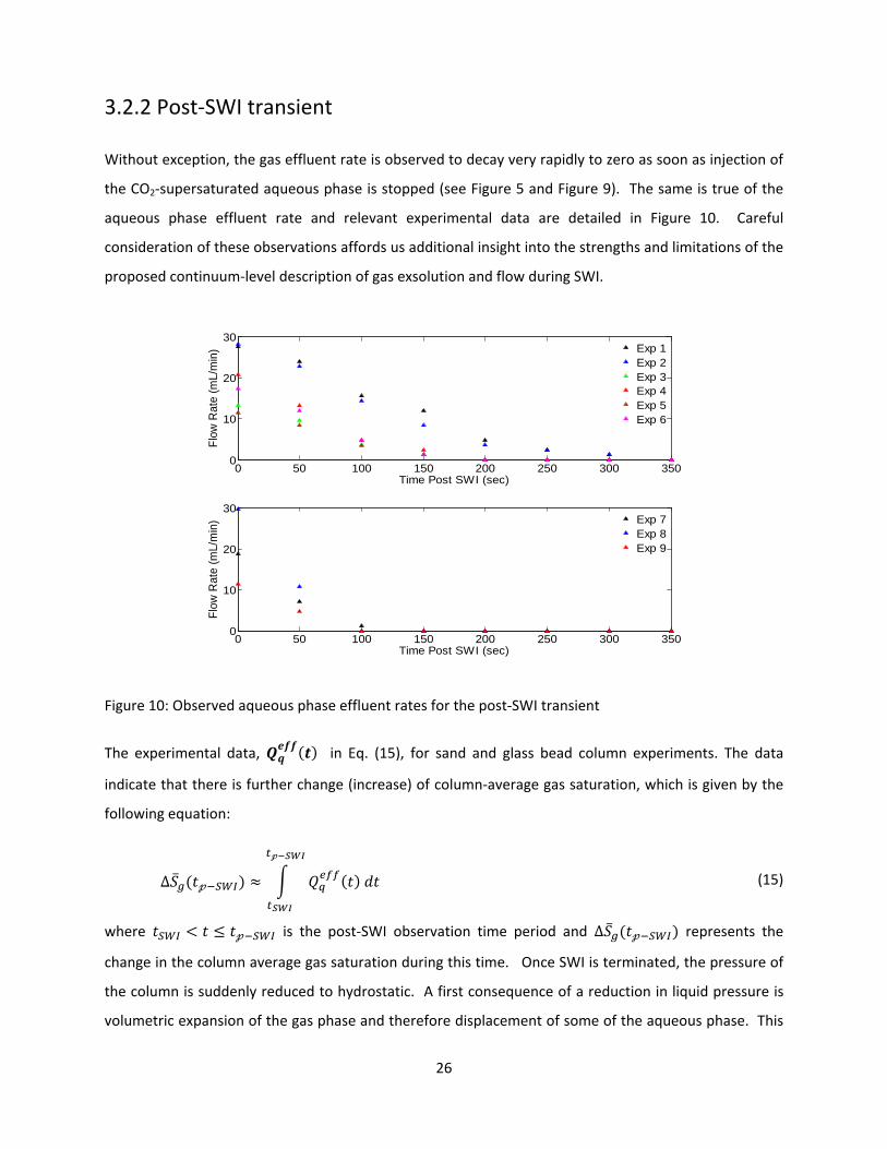
3.2.2 Post-SWI transient

Without exception, the gas effluent rate is observed to decay very rapidly to zero as soon as injection of

the CO2-supersaturated aqueous phase is stopped (see Figure 5 and Figure 9). The same is true of the

aqueous phase effluent rate and relevant experimental data are detailed in Figure 10. Careful

consideration of these observations affords us additional insight into the strengths and limitations of the

proposed continuum-level description of gas exsolution and flow during SWI.

Figure 10: Observed aqueous phase effluent rates for the post-SWI transient

The experimental data, 𝑸𝒒𝒆𝒇𝒇(𝒕) in Eq. (15), for sand and glass bead column experiments. The data

indicate that there is further change (increase) of column-average gas saturation, which is given by the

following equation:

∆𝑆�̅�(𝑡𝓅−𝑆𝑊𝐼) ≈ � 𝑄𝑞𝑒𝑓𝑓(𝑡) 𝑑𝑡

𝑡𝓅−𝑆𝑊𝐼

𝑡𝑆𝑊𝐼

(15)

where 𝑡𝑆𝑊𝐼 < 𝑡 ≤ 𝑡𝓅−𝑆𝑊𝐼 is the post-SWI observation time period and ∆𝑆�̅�(𝑡𝓅−𝑆𝑊𝐼) represents the

change in the column average gas saturation during this time. Once SWI is terminated, the pressure of

the column is suddenly reduced to hydrostatic. A first consequence of a reduction in liquid pressure is

volumetric expansion of the gas phase and therefore displacement of some of the aqueous phase. This

0 50 100 150 200 250 300 3500

10

20

30

Time Post SWI (sec)

Flow

Rat

e (m

L/m

in)

0 50 100 150 200 250 300 3500

10

20

30

Time Post SWI (sec)

Flow

Rat

e (m

L/m

in)

Exp 1Exp 2Exp 3Exp 4Exp 5Exp 6

Exp 7Exp 8Exp 9

27

consequence is accounted for in the continuum model. Other consequences are related to additional

gas phase formation (nucleation) and mass transfer-driven growth as explained below.

Both nucleation and mass transfer are processes linked to departure from thermodynamic equilibrium

as measured, for example, by the following ratio of CO2 mole fractions in the aqueous phase:

𝒮𝑓 = 𝑋𝐶𝑂2 𝑞

𝑋𝐶𝑂2 𝑞∗

(16)

where 𝑋𝐶𝑂2 𝑞 and 𝑋𝐶𝑂2 𝑞∗ represent the actual and equilibrium CO2 content of the aqueous phase and 𝒮𝑓>

1 denotes supersaturation. The degree of supersaturation varies with location and is highest at the base

of the column, where it may be readily estimated from knowledge of the aqueous phase pressure.

Assuming that the reduction of the column pressure to hydrostatic (i.e., 𝑃𝑔(𝑡𝑆𝑊𝐼) → 𝑃𝑔�𝑡𝓅−𝑆𝑊𝐼� ) is

instantaneous, the mole fraction of CO2 in the aqueous phase at the bottom of the column remains

unchanged and is equal to 𝑋𝐶𝑂2 𝑞𝑖𝑛𝑗 . Therefore, the change of ∆𝒮𝑓, the degree of supersaturation, is

realized by the sudden reduction in the pressure of the aqueous phase as follows:

∆𝒮𝑓 = 𝑋𝐶𝑂2 𝑞𝑖𝑛𝑗

𝑋𝐶𝑂2 𝑞∗ |𝑃𝑔�𝑡𝓅−𝑆𝑊𝐼�

−𝑋𝐶𝑂2 𝑞𝑖𝑛𝑗

𝑋𝐶𝑂2 𝑞∗ |𝑃𝑔(𝑡𝑆𝑊𝐼)

(17)

As shown in Table 5, reduction of the aqueous phase pressure to hydrostatic causes an increase in the

degree of supersaturation at the base of the column. In turn, this implies an increase in the driving force

for CO2 transfer from the aqueous to the gas phase (see Eq. (5)), resulting from a decrease in 𝑃𝑔 in Eq.

(10), which is accounted for in the continuum model. Another, rather distinct, implication is gas phase

formation at a number of nucleation sites not previously activated leading to the appearance of gas

phase in pores which at the conclusion of SWI contained only aqueous phase. This implication is

consistent with progressive nucleation theory [32], according to which each nucleation site is activated

at a different supersaturation threshold. By reducing the column pressure without affecting the

aqueous phase carbon dioxide concentration, the supersaturation factor was increased and caused

previously inactive nucleation sites to activate. Our ad hoc correction to the Nambi and Powers model,

𝑆𝑔𝑛𝑢𝑐 , which was found adequate for describing the rapid increase in gas saturation due to nucleation at

the initial stage of SWI, has no effect at the post-SWI stage given that the gas phase saturation in the

column is above 0.03. Table 5 shows that in every case the simulation underestimates the post-SWI gas

28

saturation growth ∆𝑆�̅�. The underestimation of gas phase saturation appears to follow a pattern closely

related to the value of supersaturation in the aqueous phase ∆𝒮𝑓 , as shown in Figure 11.

Figure 11: Gas saturation increase during SWI as a function of supersaturation.

The observed increase in gas phase saturation after SWI that is not accounted for in the simulation and

is attributed to nucleation. This is quantified as the difference between observed and simulated

increase in gas phase saturation ∆𝑆�̅�(𝑡𝓅−𝑆𝑊𝐼) and plotted against the change in the supersaturation

factor ∆𝒮𝑓 as defined by Eq. (17) and listed on Table 5. The solid line on the figure is only a guide to the

eye. This finding is consistent with progressive nucleation theory, which states that nucleation sites can

become active if a sufficient supersaturation factor is achieved [32]. It also illustrates a limitation in the

way the effects of nucleation are presently handled in the continuum model.

29

Table 3: Properties of packed columns used in CO2-SWI experiments.

Experiment ID Packing

Permeability

𝑲 �𝐦𝟐�

Average

Particle Size

𝒅𝒑 [𝝁𝒎]

Porosity

𝝓 [−] 𝑩𝒐 [−]

1 Sand 1.12×10-11 169 0.367 1.52x10-6

2 Sand 1.12×10-11 169 0.367 1.52x10-6

3 Sand 2.91×10-11 305 0.350 3.96x10-6

4 Sand 4.05×10-11 324 0.351 5.51x10-6

5 Sand 3.82×10-11 324 0.352 5.20x10-6

6 Sand 3.82×10-11 324 0.352 5.20x10-6

7 Glass beads 5.65×10-11 254 0.384 7.68x10-6

8 Glass beads 5.65×10-11 254 0.384 7.68x10-6

9 Glass beads 5.65×10-11 254 0.384 7.68x10-6

Table 4: Experimental control variables and measurements.

Experiment

ID

Control Variables Measurements

𝑸𝒒𝒊𝒏𝒋

[𝐦𝐋/𝐦𝐢𝐧]

𝑿𝑪𝑶𝟐 𝒒𝒊𝒏𝒋

[−]

𝑷𝒒(𝒕𝑺𝑾𝑰)

[𝐤𝐏𝐚]

𝑷𝒒�𝒕𝓹−𝑺𝑾𝑰�

[𝐤𝐏𝐚]

𝑸𝒈𝒆𝒇𝒇(𝒕𝑺𝑾𝑰)

[𝐦𝐋/𝐦𝐢𝐧]

1 27.60 0.002902 188.5 118.6 87.23

2 28.15 0.002599 188.5 118.6 76.14

3 13.20 0.002076 131.7 118.6 26.20

4 20.82 0.002099 133.8 118.6 44.28

5 11.49 0.001798 128.7 118.6 20.16

6 17.40 0.002111 135.8 118.6 37.76

7 18.72 0.001992 128.7 118.6 37.13

8 29.66 0.002005 135.8 118.6 58.16

9 27.60 0.001804 126.7 118.6 20.02

30

Table 5: Column-average gas phase saturation and inlet aqueous phase CO2-supersaturation.

Experiment observed predicted prediction error

ID ∆𝓢𝒇 ∆𝑺�𝒈 ∆𝑺�𝒈 ∆𝑺�𝒈

𝒕𝟎 ≤ 𝒕 ≤ 𝒕𝑺𝑾𝑰 𝒕 = 𝒕𝟎 𝒕 = 𝒕𝑺𝑾𝑰 𝒕 = 𝒕𝑺𝑾𝑰

1 2.42 0.173 0.163 0.010

2 2.16 0.130 0.158 -0.028

3 2.47 0.152 0.150 0.002

4 2.46 0.177 0.154 0.023

5 2.19 0.167 0.144 0.023

6 2.44 0.169 0.152 0.017

7 2.43 0.140 0.146 -0.006

8 2.32 0.145 0.149 -0.003

9 2.24 0.148 0.140 0.008

𝒕𝑺𝑾𝑰 < 𝑡 ≤ 𝒕𝓹−𝑺𝑾𝑰 𝒕 > 𝑡𝑺𝑾𝑰 𝒕 = 𝒕𝓹−𝑺𝑾𝑰 𝒕 = 𝒕𝓹−𝑺𝑾𝑰

1 1.42 0.104 0.039 0.065

2 1.28 0.094 0.042 0.052

3 0.27 0.031 0.007 0.024

4 0.32 0.045 0.005 0.040

5 0.19 0.028 0.003 0.025

6 0.35 0.040 0.005 0.035

7 0.21 0.024 0.004 0.020

8 0.33 0.034 0.007 0.027

9 0.15 0.013 0.003 0.010

31

Chapter 4

4. Oil Recovery and Flow during Supersaturated Water Injection

in Porous Media:

Column Experiments and Continuum Modeling

4.1 Experimental Methods and Supplemental Formulation

The experiments conducted in Chapter 3 were originally 3-phase experiments, but it was immediately

evident that gas, water and oil flowing in a porous media were extremely complicated to understand let

alone predict. In order to properly understand the system, 2-phase gas and water experiments were

conducted. From previous research, it is known that a mobile gas phase in the presence of a mobile

aqueous phase can induce mobility in an oil phase beyond its water-flood residual [35]. It is

hypothesized that the gas phase in some way carries or displaces oil during this process. With

knowledge of gas phase mobility in porous media it is possible to determine the oil phase mobility. An

objective of this chapter is to modify Stone’s Method applicable to oil phase mobility in 3-phase systems

so that it is predictive for 3-phase systems under the influence of SWI.

The approach is based on the following premises: (1) Using the simulation of 2-phase systems an

understanding was developed of gas and aqueous phase interactions in unconsolidated porous media.

It is hypothesized that a third phase will not considerably affect the interaction and mobility of the

aqueous and gas phases. If this hypothesis holds, it will be possible to characterize the mobility and flow

of oil in a 3-phase system. (2) An adjustable function will be used instead of Stone’s method due to its

inadequacy in the experimental range. The function which determines oil phase mobility is dependent

on the 3-phase saturation distribution. Consequently, it depends on adjustable parameters such as oil

phase water flood residual 𝑆𝑛𝑞𝑟, critical oil phase residual 𝑆𝑛𝑟𝑐, and residual gas phase saturation 𝑆𝑔𝑟.

Experimental data will be used to calibrate each simulation to develop a model capable of predicting

future 3-phase systems.

32

4.1.1 Experimental Methods

Chapter 4 experiments were conducted with the same laboratory equipment as the Chapter 3

experiments. The column is prepared in a manner consistent with that of Chapter 3. When the column

properties are known the system is flooded with oil by adding kerosene to the top of the column and

allowing water to drain from the bottom. This creates a system with water at its irreducible level and

the remaining pore space occupied by oil. The irreducible water saturation has been independently

determined by Leverett for sand and Ioannidis for glass bead systems and refers to the minimum water

saturation that can be achieved, via drainage in this case. The system was then flooded with water, first

at 1 mL/min and then 3 mL/min both until a pore volume has been injected into the column, effectively

displacing some oil from the system and entrapping oil in the form of ganglia throughout the porous

media. The oil saturation at the completion of this process is known as the water flood residual oil

saturation. Figure 12 depicts the experimental setup.

Figure 12: Experimental setup.

During SWI, aqueous, oil and gas phase effluents from the column were sent to a graduated pipette

acting as a phase separator. The gas phase flows to the top of the separator through a mass flow meter

and the liquid phases remain in the glass pipette. Due to buoyancy, the oil floated on top of the water

where its volume was measured using a calibrated pipette. Water was collected from the base of the

separator in a beaker and weighed continuously using a digital balance connected to a computer. A

mass flow meter (Omega, model FMA3304), used to measure the effluent rate of the gas which

33

consisted of almost pure CO2 and a pressure transducer (Validyne, model DP10-44) used to monitor the

aqueous phase pressure at the base of the column were also interfaced with a computer.

At the start of each experiment, the column was maintained at zero gas saturation and at water flood

residual oil saturation with the remaining pore space occupied by aqueous phase. Upon initiation of

SWI, the supersaturated aqueous phase enters the column and carbon dioxide bubbles instantaneously

form via nucleation; mass transfer to the gas phase continues until the gas phase pressure exceeds

entrapping capillary pressures to allow for gas phase mobilization, fragmentation and coalescence as

discussed in Chapter 3. The developing gas phase volumetrically displaces both trapped oil and free

aqueous phase along its path causing flow throughout the column. Due to its connected nature, the

aqueous phase is easily displaced and an increase in aqueous phase effluent is observed during the

development of gas phase saturation. The disconnected oil phase does not immediately allow free-

phase oil to flow out of the system; however, experimental results indicate that the oil phase is

mobilized during the early stages of gas saturation development.

Experimental focus is divided into two areas of interest: short term gas saturation development and long

term oil recovery. Short term experiments focus on a large number of measurements made over the

time taken to produce gas saturation throughout the column, which is typically less than 1 pore volume

injected. During this time, the average gas saturation of the column can be determined based on the

aqueous phase effluent as detailed in Chapter 3. Long-term experiments focus on the ability of SWI to

mobilize the oil phase contained in unconsolidated porous media. When the long-term experiments

were conducted, the importance of data collection over the first pore volume injected was not known;

subsequently gas phase saturation was not measured. Short-term experiments were used to calibrate

gas phase relative permeability parameters to produce accurate long-term simulations. Long-term

experiments are conducted until a large amount of oil phase is collected and the oil phase mobility is

reduced near zero, typically over the injection of 100-200 pore volumes. Experimental data can be

found in Tables 6 and 7.

4.1.2 Aqueous/Gas Phase Relative Permeability

Aqueous 𝑘𝑟𝑞 and gas 𝑘𝑟𝑔 phase relative permeability data for both the sand and glass bead packs were

represented as follows [31]:

34

𝑘𝑟𝑞 = �𝑆𝑞 − 𝑆𝑞𝑟1 − 𝑆𝑞𝑟

�𝑛𝑞

𝑘𝑟𝑔 = �𝑆𝑔 − 𝑆𝑔𝑟1 − 𝑆𝑔𝑟

�𝑛𝑔

(18)

where 𝑆𝑞𝑟 and 𝑆𝑔𝑟 are the residual aqueous and gas phase saturations, respectively. Aqueous phase

relative permeability parameters 𝑆𝑞𝑟 and 𝑛𝑞 for packs of sand and glass beads were taken from the

experimental works of Leverett [23] and Ioannidis et al. [12], respectively. Conversely, gas phase

relative permeability parameters have been approximated for 2-phase systems in Chapter 3 and shown

to be insensitive to unconsolidated porous media material; however, this study will show that gas phase

mobility is sensitive to the presence of oil in a 3-phase system. The gas phase relative permeability

parameters 𝑆𝑔𝑟 and 𝑛𝑔 were estimated in this study and can be found in Table 2. Aqueous and gas

phase relative permeability functions are shown in Figure 13.

Figure 13: Aqueous and gas phase relative permeability curves.

Aqueous phase relative permeability is shown in black lines for sand (solid) and glass beads (dashed),

whereas gas phase relative permeability is illustrated with a blue solid line. From the simulations, it is

apparent that 3-phase gas mobility can be accurately modeled by slightly altering the 2-phase gas phase

relative permeability function proposed in Chapter 3. By changing the residual gas saturation, 𝑆𝑔𝑟, the

simulation is able to achieve accurate gas saturation, mobility and effluent rates throughout the entirety

of experiment. As shown in Table 3, the value of 𝑆𝑔𝑟 obtained for both sand and glass bead is 0.18,

which is higher than the value obtained for the 2-phase case. It is not precisely known why the residual

gas saturation increases when 3-phases are present; however, it is likely that the presence of the oil

0 0.1 0.2 0.3 0.4 0.5 0.6 0.7 0.8 0.9 1-8

-7

-6

-5

-4

-3

-2

-1

0

Aqueous Phase Saturation, Sq [dim]

Dra

inag

e R

elat

ive

Perm

eabi

lity

[dim

]

35

phase in unconsolidated porous media disrupts gas phase flow. Due to their disconnected nature, oil

ganglia are difficult to displace in the subsurface and may increase the overall resistance to gas flow.

4.1.3 Oil Phase Relative Permeability Function

Oil phase relative permeability in 2-phase systems has been studied considerably; however, it has not

been sufficiently studied for 3-phase (oil, gas and water) systems. One study of particular importance to

the petroleum industry led to Stone’s development of a 3-phase oil relative permeability function [17].

𝑘𝑟𝑛 = 𝑘𝑟𝑛𝑐𝑞 ��𝑘𝑟𝑛𝑞𝑘𝑟𝑛𝑐𝑞

+ 𝑘𝑟𝑞��𝑘𝑟𝑛𝑔𝑘𝑟𝑛𝑐𝑞

+ 𝑘𝑟𝑔� − �𝑘𝑟𝑞 + 𝑘𝑟𝑔��

(19)

where 𝑘𝑟𝑛𝑐𝑞 is the constant oil relative permeability at connate water conditions, 𝑘𝑟𝑛𝑞 is the oil relative

permeability on the oil-water Corey curve, 𝑘𝑟𝑞 is the aforementioned aqueous phase relative

permeability, 𝑘𝑟𝑛𝑔 is the oil relative permeability on the oil-gas Corey curve, and 𝑘𝑟𝑔 is the

aforementioned gas phase relative permeability [17].

To accurately predict oil mobility in three phases, Stone proposed that events at both oil-water and oil-

gas interfaces play roles which in turn implies that oil mobility is dependent on oil, gas, and aqueous

phase saturations at any given time and position. Stone proposed a method for determining oil relative

permeability that has been the cornerstone of 3-dimensional 3-phase modeling since its development

and has been validated in a comprehensive literature review by Fayers and Matthews [35].

Unfortunately, the method has only been verified in high oil saturation and high gas saturation systems.

During SWI, the system will typically achieve gas saturation no higher than 30% and oil saturation near

water flood residual values less than 20%. Unfortunately, literature data associated with Fayers’ and

Matthews’ review dealt with oil mobility in regions of high gas saturation and/or high oil saturation,

regions which are not applicable to SWI in this study. The simulation was unable to reproduce

experimental SWI results when using Stone’s method to determine oil phase mobility. Numerically,

Stone’s method is not stable in the saturation range achieved by SWI in 3-phase systems because it does

not smoothly approach a value of zero at low oil saturations; instead, the method produces negative

values that have no physical representation.

To remedy the inadequacies of Stone’s method, this paper will introduce a new relative permeability

function that allows for accurate simulation of long-term SWI experiments and also approximates

Stone’s method at the conditions for which it has been shown to be valid. A function was developed on

36

the basis of two main contributions to oil mobility: 1) the 2-phase oil-water relative permeability table

contributes to the mobility of the oil phase when saturations are above water flood residual levels and

2) a mobile gas phase in the presence of a mobile aqueous phase increases the oil phase mobility in

unconsolidated porous media. This function is introduced in equations 20-21.

𝑘𝑟𝑛 = 𝑘𝑟𝑛𝑞 + Ω𝑆𝑛𝑟𝑐 ∙ 𝑘𝑟𝑔 ∙ 𝑘𝑟𝑛𝑐

where,

𝑘𝑟𝑛𝑞 = �𝑆𝑛 − 𝑆𝑛𝑞𝑟1 − 𝑆𝑛𝑞𝑟

�𝑛𝑛

Ω𝑆𝑛𝑟𝑐 = (1 − 𝑘𝑟𝑛𝑐) ∙ �1 − 𝑘𝑟𝑔� ∙ Λ

𝑘𝑟𝑛𝑐 = �𝑆𝑛 − 𝑆𝑛𝑟𝑐1 − 𝑆𝑛𝑟𝑐

�𝑛𝑛

(20)

(20a)

(20b)

(20c)

Equation 20 (with equations a, b and c) determines the oil phase mobility based on a 2-phase system,

𝑘𝑟𝑛𝑞, with the added effects of gas phase mobility for a 3-phase system, Ω𝑆𝑛𝑟𝑐-𝑘𝑟𝑔-𝑘𝑟𝑛𝑐. The value 𝑘𝑟𝑛𝑐 is

the critical oil relative permeability developed for this study, and Ω𝑆𝑛𝑟𝑐 is a multiplier to determine the

effect of gas phase mobility on oil phase mobility and was also developed for this study. The value 𝑆𝑛𝑞𝑟

is the water flood residual saturation of oil and 𝑆𝑛𝑟𝑐 is the critical residual saturation of oil, which is less

than 𝑆𝑛𝑞𝑟 during SWI. 𝑆𝑛𝑟𝑐 is a parameter introduced in this study and was experimentally inferred;

experiments appear to produce significantly less oil effluent when residual oil content is close to 6% for

all experiments, which may indicate a lower boundary to the success of this technology. The value Λ is

an adjustable parameter introduced to control the effect of gas phase mobility on oil phase mobility in

the model. Oil phase mobility as predicted by the oil-water Corey curve, 𝑘𝑟𝑛𝑞 , will not be affected

unless the gas phase present in the system is mobile, which is consistent with previous research [36].

Due to the complexity of the system, a modifiable multiplier such as Ω𝑆𝑛𝑟𝑐 was required because a single

set of parameters was not able to simulate all long-term oil experiments. It was necessary to control gas

phase mobility effects on oil phase mobility for each experiment in order to accurately fit experimental

data.

37

4.2 Results and Discussion

In the simulations reported here, only the gas relative permeability parameter 𝑆𝑔𝑟 and the oil relative

permeability parameters 𝑆𝑛𝑟𝑐 and Λ were considered adjustable. Every other parameter was

independently measured or estimated, similar with the previous chapter except the value 𝑛𝑔 was

assumed from Chapter 3. In what follows, the observations and numerical results which pertain to the

short-term and long-term experiments are discussed. Short-term experimental results include the first 2

pore volumes injected during the long-term experiments; therefore, it is hoped that the short-term

experimental results can be used to better understand the long-term experiments. Subsequently,

continuum model predictions for both short and long term experiments are delineated.

4.2.1 Short-term Experiments and Simulations

Short term experiments were designed to collect large amounts of data during the development of gas

saturation throughout the column. Study of this timeframe is necessary to properly understand how the

presence of an oil phase changes the gas phase characteristics from a 2-phase system to a 3-phase

system. The history of one short term experiment can be observed in Figure 14.

Figure 14: Experiment 15 short-term gas and aqueous phase effluent curves.

It is apparent that the fitted model is capable of reproducing the aqueous and gas phase effluents in a 3-

phase system. However, short-term calculations have indicated that the gas phase mobility in a 3-phase

0 0.1 0.2 0.3 0.4 0.5 0.6 0.7 0.8 0.9 10

10

20

30

40

50

60

70

80

Gas Phase Effluent

Aqueous Phase Effluent

Pore Volumes Injected

Flow

Rat

e (m

L/m

in)

38

system differs from that in the 2-phase experiments. To properly fit both short and long term

experiments, the gas phase relative permeability curve had to be slightly adjusted using experimental

calibration. Although this may seem a small detail of the experiment, it may in fact provide a clue as to

how the oil phase is mobilized by the presence of a mobile gas phase. The 3-phase experiments show a

significant increase in gas phase saturation, which indicates that the presence of the oil phase is

restricting gas phase flow. In Experiment 8 (2-phase) the gas phase effluent is around 58 mL/min

producing an average gas phase saturation of 14-15%, whereas Experiment 15 (3-phase) has a gas phase

effluent of only 50 mL/min producing an average gas saturation of 21-22%. Explanations for this

observation include reduced hydraulic conductivity during volumetric displacement of aqueous phase by

gas phase, oil phase ganglia disrupting gas flow channel creation and difficulties displacing ganglia due

to their disconnected nature. Each aforementioned explanation would result in an increase in

entrapping pressure of a gas bubble inside a pore, which could cause an increase in capillary pressure

and result in higher gas phase saturation.

During short-term experiments, the oil phase was mobilized as shown in figure 15.

Figure 15: Experiment 15 short-term oil recovery experiment and simulation.

During the first pore volume injected there is a measureable and relatively large volume of oil phase

effluent. The oil effluent is likely caused by oil bank formation along the developing gas saturation front

that is described in Chapter 2. As the gas phase first moves through the column it volumetrically

displaces and redistributes both oil and aqueous phases. By redistributing disconnected ganglia, it is

possible that buoyant clusters can form and be propelled out of the system buoyantly, by the gas

10-1 100 1010.12

0.125

0.13

0.135

0.14

0.145

0.15

Pore Volumes Injected (log)

Oil

Rem

aini

ng (%

PV)

39

saturation front. The oil phase effluent is produced at the same time as the first gas phase effluent,

which is sufficient evidence to support this theory.

Figure 15 shows that oil phase recovery during this time is not accurately computed by the model. The

relative permeability function as described in Section 4.1.2 was designed to incorporate oil mobility for

2-phase oil-water systems and include the effects of gas phase mobility on the oil phase mobility in 3-

phase systems. Unfortunately, the factors affecting oil phase mobility are likely dynamic and so can

change throughout long-term experiments. It is possible to accurately model both short-term and long-

term oil production; however, this would require the use of a step function and further complicate the

simulation. Concessions were made to focus on long-term oil recovery instead because field-scale

applications typically last much longer than 10 pore volumes.

4.2.2 Long-term Experiments and Simulations

Long-term experiments were designed to collect large amounts of data throughout an experiment

consisting of more than 200 pore volumes injected. Study of this timeframe is necessary to properly

understand how the introduction of mobile gas and aqueous phases via SWI can produce mobility in an

otherwise immobile disconnected oil phase. The results contained in the long-term experiments can be

found in Table 7. The variations of oil-phase saturations obtained during these experiments are shown

in Figure 16.

The aqueous and gas phase effluents are not displayed because they are not the focus of this time

period, but they were accurately by the model. Relative permeability and continuum-scale concepts are

not capable of exactly modeling the dynamics observed during experiment; however, concessions must

be made in order to scale a pore-scale process up to the continuum-scale. Each long-term experiment

has been accurately predicted by simulation; however, all of the experiments could not be predicted by

a single relative permeability function. Table 8 shows simulation characteristics and model parameters

obtained for each experiment. Model parameters such as Λ are able to control the effect that gas phase

mobility has on the oil phase.

40

Figure 16: Experiments 10-14 long-term oil recovery experiments (solid lines) and simulations (symbols).

Figure 16 show that consistent oil effluent curves are obtained for the various experiments, which allow

continuum-scale relative permeability concepts to be used. It is apparent that gas phase mobility and oil

phase mobility are highly correlated, but the physical mechanism at work is not completely understood.

A high density band of results and simulations, which is indicative of the high correlation between gas

phase and oil phase mobility. The figure is a normalized representation of experimental and simulation

results; it also indicates a very strong relationship between percent of oil phase remaining and pore

volumes of aqueous phase injected.

Although the end-point average oil phase saturation is accurately simulated for each experiment,

effluent observations are unable to show the remaining oil distribution in the column at the end of an

experiment. To truly determine if the simulation is capable of predicting oil phase flow, the residual

saturations throughout the column must be matched. To determine the end of experiment saturation

gradient, porous media were carefully removed from the column and analyzed with gas chromatograph

technology, as detailed in Li [36]. The columns were later reconstructed virtually with average oil

saturation data at the various locations. One such reproduction can be found in Figure 17.

Pore volumes injected

Col

umn

aver

aged

oils

atur

atio

n

10-1 100 101 102

0.06

0.08

0.1

0.12

0.14

0.16

0.18

10101111121213131414

Experiment ID

41

The nearly homogeneous distribution of oil phase at the end of SWI experiments matches simulation

results very well. Experimental results are consistent with simulation techniques; however, the

simulation is forced to produce a nearly homogeneous end-point by boundary conditions and

assumptions such as a critical saturation for oil mobility, 𝑆𝑛𝑟𝑐.

Figure 17: Example of saturation distribution produced at end of SWI oil recovery [36].

4.2.3 Enouy Approximation of Stone’s Method

The main goal of this paper is to produce a function capable of predicting oil mobility at low oil

saturations during SWI; however, a function capable of predicting oil mobility for all saturations of gas,

oil and water phases would be more useful. Isoperm Contour plots of Stone’s Method and the Enouy

approximation of Stone’s Method were created to show their similarities. Figure 18 shows the

dependence of 𝑘𝑟𝑛 on oil and gas-phase saturations based on Stone’s Method, while Figure 19 presents

the results obtained using the Enouy Approximation.

0

20

40

60

80

100

120

140

160

7.23%8.66%9.67%7.38%7.62%

7.52%

5.56%

6.61%

7.56%8.30%8.06%6.64%

42

Figure 18: Stone’s Method for producing oil phase relative permeability in 3-phase systems.

Srn = 0.14, Srq = 0.20, Srg = 0.18, krncq = 0.6723, krng = �Sn − 0.201 − 0.20

�1.8

Simulations were conducted with Stone’s Method approach for determining relative permeability of oil

phase in 3-phase systems; however, any oil mobility that was created was large enough to predict all oil

effluent within the first 10 pore volumes. Stone’s Method cannot predict SWI experiments for flow in

1D columns.

Gas phase saturation [-]

Oil

phas

esa

tura

tion

[-]

0 0.2 0.4 0.6 0.8 10

0.2

0.4

0.6

0.8

1

0.90.80.70.60.50.40.30.20.10.0

Oil phaserelativepermeability [-]

0.80

0.70

0.60

0.50

0.40

0.30

0.20

0.100.05

0.01

Gas phase saturation [-]

Oil

phas

esa

tura

tion

[-]

0 0.2 0.4 0.6 0.8 10

0.2

0.4

0.6

0.8

1

43

Figure 19: Enouy approximation of Stone’s Method for oil phase relative permeability in 3-phase

systems.

𝑺𝒏𝒒𝒓 = 𝟎.𝟏𝟒,𝚲 = 𝟐.𝟎,𝑺𝒏𝒓𝒄 = 𝟎.𝟎𝟔.

By comparing the figures side-by-side it is difficult to tell how similar the two methods are; however, a

third contour plotting the absolute difference of Enouy and Stone can be found in Figure 20.

Gas phase saturation [-]

Oil

phas

esa

tura

tion

[-]

0 0.2 0.4 0.6 0.8 10

0.2

0.4

0.6

0.8

1

0.90.80.70.60.50.40.30.20.10.0

Oil phaserelativepermeability [-]

0.8000

0.7000

0.6000

0.5000

0.4000

0.3000

0.2000

0.1000

0.0500

0.01000.0050

0.00100.00050.0001

Gas phase saturation [-]

Oil

phas

esa

tura

tion

[-]

0 0.2 0.4 0.6 0.8 10

0.2

0.4

0.6

0.8

1

44

Figure 20: Difference between Enouy approximation and Stone’s Method for oil phase relative

permeability in 3-phase systems.

The majority of contour lines, and therefore difference between the methods are smaller than 0.06, a

reasonable difference, which is a testament to the similarity between the two methods. Obviously, the

difference between the methods is large at low oil and high gas saturations – the region in which Stone’s

Method performs poorly.

𝑫𝒊𝒇𝒇𝒆𝒓𝒆𝒏𝒄𝒆 = 𝒌𝒏𝒓,𝑺𝒕𝒐𝒏𝒆 − 𝒌𝒏𝒓,𝑬𝒏𝒐𝒖𝒚 (21)

Gas phase saturation [-]

Oil

phas

esa

tura

tion

[-]

0 0.2 0.4 0.6 0.8 10

0.2

0.4

0.6

0.8

1

0.330.300.270.240.210.180.150.120.090.060.030.00

-0.03

difference inrelativepermeability [-]

-0.05-0.04-0.03

-0.02-0.01

0.000.010.02

0.03

0.04

0.05-0.01

0.010.00

0.020.03

0.05

0.04

Gas phase saturation [-]

Oil

phas

esa

tura

tion

[-]

0 0.2 0.4 0.6 0.8 10

0.2

0.4

0.6

0.8

1

45

Table 6: Properties of packed columns SWI experiments.

Experiment

ID Packing

Permeability

𝑲 [𝐝𝐚𝐫𝐜𝐲] Porosity 𝝓 [−]

Water Flood

Residual Oil

𝑺𝒏𝒒𝒓 [-]

10 Sand 11.4 0.387 0.133

11 Sand 09.1 0.369 0.149

12 Sand 31.2 0.380 0.152

13 Sand 29.4 0.350 0.153

14 Sand 41.9 0.358 0.162

15 Sand 44.8 0.365 0.141

16 Glass beads 64.4 0.395 0.134

Table 7: Experimental observations.

Experiment ID

Duration 𝑸𝒒−𝒂𝒗𝒈𝒊𝒏𝒋

[𝐦𝐋/𝐦𝐢𝐧]

𝑸𝒈−𝒂𝒗𝒈𝒆𝒇𝒇

[𝐦𝐋/𝐦𝐢𝐧] 𝑺�𝒈[−]

Fraction

Oil Recovery

[%]

10 Long 35.2 67.6 - 0.442

11 Long 28.5 56.6 - 0.581

12 Long 25.6 53.2 - 0.511

13 Long 26.5 58.1 - 0.590

14 Long 26.3 56.6 - 0.599

15 Short 23.7 50.9 0.214 0.060

16 Short 24.3 50.6 0.198 0.047

46

Table 8: Simulation results and parameters.

Simulation ID

Duration 𝑺�𝒈[−]

Fraction

Oil Recovery

[%]

Oil Mobility

Multiplier

𝚲[−]

10 Long 0.197 0.453 2.5

11 Long 0.199 0.551 6

12 Long 0.203 0.532 2

13 Long 0.205 0.626 4.5

14 Long 0.203 0.574 5

15 Short 0.201 0.075 2

16 Short 0.198 0.055 2

47

Chapter 5

5. Conclusions

5.1 Gas Exsolution and Flow during Supersaturated Water Injection in

Porous Media

A first investigation of the process is conducted of CO2-supersaturated water injection (SWI) in water-

saturated porous media by means of experiments in homogeneous columns packed with glass beads or

silica sand and continuum-scale simulation. This study addressed aspects of two-phase flow and mass

transfer at the macroscopic scale, strengthening and extending a number of conclusions reached in the

first part of this work [1], where CO2-supersaturated water injection was studied by pore network

simulation. A multiphase compositional model (CompFlow-SWI) was employed to interpret the

experimental observations, leading to the following conclusions:

• Initial formation (nucleation) and growth of the CO2 gas phase during SWI is associated with the

development of an exsolution zone of finite extent near the point of injection. Rate-limited transfer

of CO2 from the aqueous to the gas phase is adequately described at the macroscopic scale by a

published correlation due to Nambi and Powers [19].

• Gas phase accumulating within the exsolution zone becomes mobile at a critical value of gas

saturation which, for the media studied in this work, is close to the breakthrough gas saturation for

drainage of the aqueous phase (ca. 0.14). Advection of the gas phase is consistent with the

advancement of a sharp front and can be predicted by the classical extension of Darcy’s law to two-

phase flow. The associated gas phase relative permeability is determined and found to be

insensitive to changes in particle size and injection flow rate.

The finding that displacement of the aqueous phase by gas is compact at the macroscopic scale is

consistent with a pore-level description of the SWI process, according to which gas phase propagation

under conditions of small Bond number results from repeated mobilization, fragmentation and

coalescence of large gas clusters (i.e., large ganglion dynamics) driven entirely by mass transfer. The

apparent success of a Darcy-based model of gas phase mobility hinges on the existence of a

representative elementary volume (REV) for gas saturation, which is assured by the uniform nature of

48

nucleation and mass transfer-driven growth of a gas phase in porous media. This is likely a significant

advantage of SWI over gas sparging, which generally results in channelized gas flow.

5.2 Oil Recovery and Flow during Supersaturated Water Injection in

Porous Media

An investigation was conducted to determine how the process of CO2-supersaturated water injection

(SWI) can produce mobility in a disconnected oil phase that was previously immobile. Experiments were

carried out in homogeneous columns packed with both silica sand and glass beads with a water flood

residual oil phase; SWI was initiated to produce oil, gas and aqueous phase effluents and was used to

calibrate a continuum-scale simulation. This study addressed aspects of 3-phase flow during SWI that

has not been previously investigated. A new relative permeability relationship for gas phase in the

presence of oil and water was developed, which is slightly different from the relationship developed for

2-phase flow. Stone’s method for 3-phase oil relative permeability was shown to be inadequate for

simulating SWI systems and a new function was developed. The function accurately predicts relative

permeability in areas where Stone is valid as well as the low oil saturations applicable to SWI. A

multiphase compositional model (CompFlow-SWI) was employed to interpret the experimental

observations, leading to the following conclusions:

• Gas phase flow in porous media was shown to be sensitive to the presence of an oil phase for both

sand and glass bead packed columns. The average gas phase saturation was much higher for 3-

phase systems than 2-phase systems. The relative permeability curve for gas phase flow had to be

altered in order to match experimental results, but the new relationship was able to accurately

predict each 3-phase experiment. It is concluded that a residual disconnected oil phase increases

resistance to gas phase flow, although the exact mechanism is yet unknown.

• Oil phase flow cannot be adequately described by Stone’s Method during SWI. To allow for accurate

reproduction of experimental results a new relative permeability function was developed. The new

function is able to accurately predict oil relative permeability as the oil phase approached immobile

saturations. The function is also able to accurately reproduce Stone’s Method predictions for high

oil saturations and high gas saturations.

A disconnected oil phase can be mobilized with supersaturated water injection and accurately predicted with a continuum-scale modeling approach.

49

References

1. Zhao W, Ioannidis MA. Gas exsolution and flow during supersaturated water injection in porous

media: I. Pore network modeling, submitted for publication.

2. Avraam DG, Payatakes AC. Flow regimes and relative permeabilities during steady-state 2-phase

flow in porous media. J Fluid Mech 1995; 293:207-236.

3. Avraam DG, Payatakes AC. Generalized relative permeability coefficients during steady-state 2-

phase flow in porous media and correlation with the flow mechanisms. Transp Porous Media 1995;

20:135-168.

4. Fry VA, Selker JS, Gorelick SM. Experimental investigations for trapping oxygen gas in saturated

porous media for in situ bioremediation. Water Resour Res 1997; 33(12):2687-2696.

5. Li TMW, Ioannidis MA, Chatzis I. Recovery of non-aqueous phase liquids from ground sources.

United States patent #7300227, 2007.

6. Bass DH, Hastings NA, Brown RA. Performance of air sparging systems: a review of case studies. J

Hazard Mater 2000; 72:101-119.

7. Nelson LC, Barker J, Li T, Thomson N, Ioannidis M, Chatzis I. A field trial to assess the performance

of CO2-supersaturated water injection for residual volatile LNAPL recovery. J Contam Hydrol. 2009;

109:82-90.

8. Brooks MC, Wise WR, Annable MD. Fundamental changes in in-situ air sparging flow patterns.

Ground Water Monit Rem 1999; 19(2):105-113.

9. Chen M-R, Hinkley RE, Killough JE. Computed tomography imaging of air sparging in porous media.

Water Resour Res 1996; 32(10):3013-3024.

10. Elder CR, Benson CH. Air channel formation, size, spacing and tortuosity during air sparging.

Ground Water Monit Rem 1999; 19(3):171-181.

11. Geistlinger H, Lazik D, Krauss G, Vogel H-J. Pore-scale and continuum modeling of gas flow pattern

obtained by high-resolution optical bench-scale experiments. Water Resour Res 2009; 45.

doi:10.1029/2007WR006548.

12. Ioannidis MA, Chatzis I, Lemaire C, Perunarkilli R. Unsaturated hydraulic conductivity from nuclear

magnetic resonance measurements. Water Resources Research 2006; 42: W07201,

doi:10.1029/2006WR004955.

13. Johnson RL, Johnson PC, McWhorter DB, Hinchee RE, Goodman I. An overview of in situ air

sparging, Ground Water Monit Rem 1993; 13(4):127-135.

50

14. Selker JS, Niemet M, McDuffie NG, Gorelick SM, Parlange JY. The local geometry of gas injection into

saturated homogeneous porous media. Transp Porous Media 2007; 68(1):107-127.

15. Stauffer F, Kong XZ, Kinzelbach W. A stochastic model for air injection in porous media. Adv Water

Resour 2009; 32(8):1180-1186.

16. Stohr M, Khalili A. Dynamic regimes of buoyancy-affected two-phase flow in unconsolidated porous

media. Phys Rev E 2006; 73:art. No. 036301.

17. Stone HL. Estimation of three-phase relative permeability and residual oil data. Journal of Canadian

Petroleum Technology, Oct-Dec 1973; 53-60.

18. Forsyth PA, Unger AJA, Sudicky EA. Nonlinear iteration methods for nonequilibrium multiphase

subsurface flow. Adv Water Resour 1998; 21:433-449.

19. Nambi IM, Powers SE. Mass transfer correlations for nonaqueous phase liquid dissolution from

regions with high initial saturations. Water Resour Res 2003; 39(2):1030,

doi:10.1029/2001WR000667.

20. Kashchiev D, Firoozabadi A. Kinetics of the initial stage of isothermal gas phase formation. J Chem

Phys 1993; 98(6):4690–4699.

21. Forsyth PA. A positivity-preserving method for simulation of steam injection for NAPL site

remediation. Adv Water Resour 1993; 16:351-370.

22. Unger AJA, Forsyth PA, Sudicky EA. Influence of alternative dissolution models and subsurface

heterogeneity on DNAPL disappearance times. J Contam Hydrol 1998; 30:217-242.

23. Leverett MC. Capillary behaviour in porous solids. Trans AIME 1941; 142:159–172.

24. D’Azvedo EF, Forsyth PA, Tang W-P. Towards a cost-effective high order ILU preconditioner. BIT

1992; 32:442-463.

25. Saad Y, Schultz M. GMRES: a generalized minimum residual algorithm for solving nonsymmetric

linear systems. SIAM J Sci Statist Comp 1986; 7:856-869.

26. Van der Vorst HA. Bi-CGSTAB: a fast a smoothly converging variant of BiCG for the solution of

nonsymmetric linear systems. SIAM J Sci Statist Comp 1992; 13:631-645.

27. Smith, Van Ness and Abbott. Introduction to Chemical Engineering Thermodynamics. New York, NY:

McGraw-Hill, 2005. Print.

28. Felder, Richard M., and Ronald W. Rousseau. Elementary Principles of Chemical Processes. New

York: John Wiley, 2000. Print.

29. Hines, Anthony L., and Robert N. Maddox. Mass Transfer: Fundamentals and Applications.

Englewood Cliffs, NJ: Prentice-Hall, 1985. Print.

51

30. Oxtoby, Gillis and Nachtrieb. Principles of Modern Chemistry. Toronto, CA: Thompson Learning,

2002. Print.

31. Corey AT. The interrelation between gas and oil relative permeabilities. Prod. Mon. 1954; 19(1):38-

41.

32. Li X, Yortsos YC. Visualization and simulation of bubble growth in pore networks. AIChE J 1995;

41(2):214-222.

33. Thomson NR, Johnson RL. Air distribution during in situ air sparging: an overview of mathematical

modeling. J Hazard Mater 2000; 72:265-282.

34. Tsimpanogiannis IN, Yortsos YC. The critical gas saturation in a porous medium in the presence of

gravity. J Colloid Interface Sci 2004; 270 (2):388-395.

35. Fayers and Matthews. Evaluation of Normalized Stone’s Methods for Estimating Three-Phase

Relative Permeabilities. Soc of Petro Eng Journal, April 1984; 224-231.

36. Li M. Recovery of Non-aqueous phase liquids from contaminated soil by CO2 supersaturated water

injection. University of Waterloo, Master of Applied Science thesis, 2009.

37. Ji W, Dahmani A, Ahfeld DP, Lin JD, Hill E. Laboratory study of air sparging: Air flow visualization.

Ground Water Monit Rem 1993; 13(4):115-126.

38. Klotz D, Seiler K-P, Moser H, Neumaier F. Dispersivity and velocity relationship from laboratory and

field experiments. J Hydrol 1980; 45:169-184.

39. Buckley SE, Leverett MC. Mechanism of fluid displacements in sands. Trans AIME 1942; 146:107–

116.