continuum mechanics themodynamics the equations dr. m ... · strain tensor stress tensor...
TRANSCRIPT

Strain tensor
Stress tensor
Themodynamics . . .
The equations . . .
Fluid Mechanics
Home Page
Title Page
JJ II
J I
Page 1 of 56
Go Back
Full Screen
Close
Quit
Continuum Mechanics
Dr. M Ramegowda
Dept. of Physics
Govt. College (Autonomous), Mandya

Strain tensor
Stress tensor
Themodynamics . . .
The equations . . .
Fluid Mechanics
Home Page
Title Page
JJ II
J I
Page 2 of 56
Go Back
Full Screen
Close
Quit
1. Strain tensor
An elastic body under an applied load deforms into a new shape. As shown in
the figure 1 two adducent points p and q on the body displaced to p′ and q′ by
the application of the force ~F . The displacements ~u1 and ~u2 of the point p and
q are
~u1 = ~r1′ − ~r1
~u2 = ~r2′ − ~r2
~u2 − ~u1 = (~r2′ − ~r1
′)− (~r2 − ~r1)
d~u = d~r ′ − d~r
d~r ′ = d~u + d~r (1)
In terms of the cartesian components, the equation 1 can be written as√dx′1
2 + dx′22 + dx′3
2 =√
(du1 + dx1)2 + (du2 + dx2)2 + (du3 + dx3)2

Strain tensor
Stress tensor
Themodynamics . . .
The equations . . .
Fluid Mechanics
Home Page
Title Page
JJ II
J I
Page 3 of 56
Go Back
Full Screen
Close
Quit
Using general summation rule, we can write∑i
dx′i2
=∑i
(dui + dxi)2
∑i
dx′i2
=∑i
dx2i + 2duidxi + du2
i (2)
Since ui <<, the third term is quadratic in ui, can be neglected. Then the
equation 2 becomes ∑i
dx′i2
=∑i
dx2i + 2duidxi (3)
The displacement vector ui is
ui = ui(x1, x2, x3)
dui =δuiδxj
dxj (4)
Equation 4 in 3, ∑i
dx′i2
=∑i
dx2i + 2
∑i
∑j
δuiδxj
dxjdxi∑i
dx′i2
=∑i
dx2i + 2
∑i
∑j
aijdxjdxi (5)

Strain tensor
Stress tensor
Themodynamics . . .
The equations . . .
Fluid Mechanics
Home Page
Title Page
JJ II
J I
Page 4 of 56
Go Back
Full Screen
Close
Quit
r1
r′1
u2
pp′
Original shapeDeformed shape
qq′
u1
r2 r′2
x1
x2
x3
Figure 1: Deformation of an elastic body
where the tensor
aij =δujδxi

Strain tensor
Stress tensor
Themodynamics . . .
The equations . . .
Fluid Mechanics
Home Page
Title Page
JJ II
J I
Page 5 of 56
Go Back
Full Screen
Close
Quit
is the strain produced in the ith components of the deformation along jth axis
and it can be written as
aij =1
2(aij + aji) +
1
2(aij − aji)
=1
2
(δuiδxj
+δujδxi
)+
1
2
(δuiδxj− δujδxi
)= εij + ωij (6)
where
ωij =1
2
(δuiδxj− δujδxi
)is the antisymmetric part of the tensor aij, and it can be shown that it corre-
sponds to a pure rotation of the body as a whole.
εij =1
2
(δuiδxj
+δujδxi
)(7)

Strain tensor
Stress tensor
Themodynamics . . .
The equations . . .
Fluid Mechanics
Home Page
Title Page
JJ II
J I
Page 6 of 56
Go Back
Full Screen
Close
Quit
is the symmetric part of the tensor aij, and is called the strain tensor. In
cartesian components,
εij =
ε11 ε12 ε13
ε21 ε22 ε23
ε31 ε32 ε33
=
δuxδx
12
(δuxδy +
δuy
δx
)12
(δuxδz + δuz
δx
)12
(δuy
δx + δuxδy
)δuy
δy12
(δuy
δz + δuzδy
)12
(δuzδx + δux
δz
)12
(δuzδy +
δuy
δz
)δuzδz
(8)
we can that the strain tensor εij is symmetric. The eigenvectors of εij are the
principal directions of the strain, i.e., the directions where there is no shear
strain. The eigenvalues, ε11 = λ1, ε22 = λ2 and ε33 = λ3 are the principal
strains and give the unit elongations in the principal directions.
When there is no rotation, ωij = 0, and aij = εij. The equation 5 becomes,∑i
dx′i2
=∑i
dx2i + 2
∑i
∑j
εijdxjdxi (9)
If the strain tensor is diagonalize at a given point, the equation 9 can be written

Strain tensor
Stress tensor
Themodynamics . . .
The equations . . .
Fluid Mechanics
Home Page
Title Page
JJ II
J I
Page 7 of 56
Go Back
Full Screen
Close
Quit
as, ∑i
dx′i2
=∑ij
δijdxidxj + 2∑ij
εijdxidxj
=∑ij
(δij + 2εij) dxidxj
dx′i2
= (1 + 2εii) dx2i
dx′i =√
1 + 2εii dxi (10)
By using Binomial expansion and by neglecting the higher terms, the equation
10 can be written as
dx′i = (1 + εii) dxi (11)
Then the deformed volume element can be written as
dx′ dy′ dz′ = (1 + ε11)(1 + ε22)(1 + ε33) dx dy dz (12)

Strain tensor
Stress tensor
Themodynamics . . .
The equations . . .
Fluid Mechanics
Home Page
Title Page
JJ II
J I
Page 8 of 56
Go Back
Full Screen
Close
Quit
On simplifying the equation 12 and by neglecting the higher terms,
dV ′ = (1 + ε11 + ε22 + ε33) dV
=
(1 +
∑i
εii
)dV (13)
∑i
εii =dV ′ − dV
dV(14)
i.e., the sum of the diagonal components of the strain tensor becomes the relative
volume change.

Strain tensor
Stress tensor
Themodynamics . . .
The equations . . .
Fluid Mechanics
Home Page
Title Page
JJ II
J I
Page 9 of 56
Go Back
Full Screen
Close
Quit
2. Stress tensor
The internal forces which occur when a body is deformed are called internal
stresses. If no deformation occurs, there are no internal stresses. The internal
stresses are due to molecular forces, i.e. the forces of interaction between the
molecules. The molecular forces have a very short range of action.
If ~F is the force acting per unit volume on the body, the force acting on the
volume element dV is∑
i~Fi dV . Then the net force acting on the body is
~FT =
∫∫∫ ∑i
~Fi dV (15)
The total force can be obtained from an integral of a vector ~Fi, then the vector
Fi must be the divergence of a tensor of rank two, i.e. be of the form
~Fi =δσijδxj
(16)
Equation 16 in equation 15,
~FT =
∫∫∫ ∑ij
δσijδxj
dV (17)

Strain tensor
Stress tensor
Themodynamics . . .
The equations . . .
Fluid Mechanics
Home Page
Title Page
JJ II
J I
Page 10 of 56
Go Back
Full Screen
Close
Quit
According to the Green’s theorem,∫∫∫ ∑ij
δσijδxj
dV =
∫∫ ∑ij
σij dsj (18)
where dsj are the components of the surface element vector ds, directed along
the outward normal. The tensor σij is called the stress tensor. σij dsj is the ith
component of the force on the surface element dsj. The stress vector acting on
∆~F
n
∆s
Figure 2: Definition of a stress vector

Strain tensor
Stress tensor
Themodynamics . . .
The equations . . .
Fluid Mechanics
Home Page
Title Page
JJ II
J I
Page 11 of 56
Go Back
Full Screen
Close
Quit
any plane with normal n can be defined as
tn = lim∆sj→0
∆~Fi∆sj
n
tn = σijn (19)
where the tensor σij is
σij =
σ11 σ12 σ13
σ21 σ22 σ23
σ31 σ32 σ33
(20)
The diagonal elements σ11, σ22 and σ33 are the normal stresses and the off-
diagonal elements σ12, σ13, σ21, σ23, σ31 and σ32 are the shear stresses.
The moment of the forces on a portion of the body can be written as an anti-
symmetrical tensor of rank two, whose components are Fixj − Fjxi, where xi
are the co-ordinates of the point where the force is applied. Hence the moment
of the forces on the volume element dV is
Mij =
∫∫∫(Fixj − Fjxi) dV (21)

Strain tensor
Stress tensor
Themodynamics . . .
The equations . . .
Fluid Mechanics
Home Page
Title Page
JJ II
J I
Page 12 of 56
Go Back
Full Screen
Close
Quit
Substituting the expression 16 for Fi, we find
Mij =
∫∫∫ (δσikδxk
xj −δσjkδxk
xi
)dV
=
∫∫∫δ
δxk(σikxj − σjkxi) dV −
∫∫∫ (σik
δxjδxk− σjk
δxiδxk
)dV(22)
By applying Green’s theorem to the equation 22,
=
∫∫(σikxj − σjkxi) dsk −
∫∫∫ (σik
δxjδxk− σjk
δxiδxk
)dV (23)
The derivative of a co-ordinate with respect to itself is unity, and with respect
to another co-ordinate is zero. Thusδxj
δxk= δjk, where δjk is the unit tensor.
The equation 22 becomes
Mij =
∫∫(σikxj − σjkxi) dsk −
∫∫∫(σikδjk − σjkδik) dV (24)
=
∫∫(σikxj − σjkxi) dsk −
∫∫∫(σij − σji) dV
Since Mij is an integral over the surface only, the second term must vanish.
Then we must have
σij = σji

Strain tensor
Stress tensor
Themodynamics . . .
The equations . . .
Fluid Mechanics
Home Page
Title Page
JJ II
J I
Page 13 of 56
Go Back
Full Screen
Close
Quit
That is, the stress tensor is symmetrical. The moment of the forces on a portion
of the body can then be written as
Mij =
∫∫(σikxj − σjkxi) dsk (25)
In equilibrium the internal stresses in every volume element must balance, i.e.
we must have∑
i Fi = 0. Thus the equations of equilibrium for a deformed
body are ∑i
Fi =∑ij
δσijδxj
= 0 (26)
If the body is in a gravitational field, then∑i
Fi =∑ij
δσijδxj
+ ρg = 0 (27)
where ρ is the density and g is the gravitational acceleration vector, directed
vertically downwards.
If Pi be the external force on unit area of the surface of the body, so that a
force Pi df acts on a surface element df . In equilibrium, this must be balanced

Strain tensor
Stress tensor
Themodynamics . . .
The equations . . .
Fluid Mechanics
Home Page
Title Page
JJ II
J I
Page 14 of 56
Go Back
Full Screen
Close
Quit
by the force −σijdfj of the internal stresses acting on that element. Thus we
must have
Pi df = σijdfj
Pi df = σijnj df
Pi = σijnj (28)
This is the condition which must be satisfied at every point on the surface of a
body in equilibrium.

Strain tensor
Stress tensor
Themodynamics . . .
The equations . . .
Fluid Mechanics
Home Page
Title Page
JJ II
J I
Page 15 of 56
Go Back
Full Screen
Close
Quit
3. Thermodynamics of deformation
The work done W by the internal stresses in the deformed body is
W =
∫∫∫δW dV =
∫∫∫ ∑i
Fi δuidV (29)
where δW is the workdone by the internal stresses per unit volume and δui is
the displacement vector due to Fi. On substituting for Fi in terms of stress
tensor, we have∫∫∫δW dV =
∫∫∫ ∑ij
δσijδxj
δuidV
=∑ij
∫∫σijδuidsj −
∫∫∫ ∑ij
σijδ
δxj(δui) dV (30)
By considering an infinite medium which is not deformed at infinity, we make
the surface of integration in the first integral tend to infinity; then σij = 0 on

Strain tensor
Stress tensor
Themodynamics . . .
The equations . . .
Fluid Mechanics
Home Page
Title Page
JJ II
J I
Page 16 of 56
Go Back
Full Screen
Close
Quit
the surface, and the integral is zero. Then equation 30 becomes∫∫∫δW dV = −
∫∫∫ ∑ij
σij δ
(δuiδxj
)dV
= −∫∫∫ ∑
ij
σij δ
[1
2
(δuiδxj
+δujδxi
)+
1
2
(δuiδxj− δujδxi
)]dV
= −∫∫∫ ∑
ij
σijδ(εij + ωij)dV (31)
where
εij =1
2
(δuiδxj
+δujδxi
)is the strain tensor and
ωij =1
2
(δuiδxj− δujδxi
)

Strain tensor
Stress tensor
Themodynamics . . .
The equations . . .
Fluid Mechanics
Home Page
Title Page
JJ II
J I
Page 17 of 56
Go Back
Full Screen
Close
Quit
is the tensor corresponds to a pure rotation of the body. Since there is no
rotation, ωij = 0, then the equation 31 becomes∫∫∫δW dV = −
∫∫∫ ∑ij
σijδεijdV
δW = −∑ij
σijδεij
dW = −∑ij
σijdεij (32)
Equation 32 gives the workdone by the internal stresses per unit volume.
According to I law of thermodynamics,
dQ = dU + dW
dU = dQ− dW
dU = T dS +∑ij
σij δεij (from equation 32) (33)
Strain tensor
Stress tensor
Themodynamics . . .
The equations . . .
Fluid Mechanics
Home Page
Title Page
JJ II
J I
Page 18 of 56
Go Back
Full Screen
Close
Quit
The equation 33 gives the thermodynamic identity for deformed bodies. The
Helmholtz potential or free energy F of the body is
F = U − TS
dF = dU − T dS − S dT (34)
Equation 33 in equation 34 gives
dF =∑ij
σijδεij − S dT (35)
The thermodynamic potential Φ is given by
Φ = F + PV
Φ = F −∑ij
σijεij
dΦ = dF −∑ij
σij dεij −∑ij
εij dσij (36)
Equation 35 in equation 36 gives,
dΦ = −S dT −∑ij
εij dσij (37)

Strain tensor
Stress tensor
Themodynamics . . .
The equations . . .
Fluid Mechanics
Home Page
Title Page
JJ II
J I
Page 19 of 56
Go Back
Full Screen
Close
Quit
For constant entropy or constant temperature, the equations 33 and equations
35 gives
σij =
(δU
δεij
)S
=
(δF
δεij
)T
(38)
For constant temperature, the equations 37 becomes
εij = −(δΦ
δσij
)T
(39)
3.1. Hooke’s law
Consider an isotropic body in small deformation at constant temperature through-
out the body. Then the stress tensor is given by
σij =
(δF
δεij
)T
(40)
Thus free energy F be an explicit function of T and εij. At constant tempera-
ture, it can be expand in powers of εij using Taylor’s series.
F = Fo +∑ij
Cijεij +1
2!
∑ij
Cijklεijεkl + ............... (41)

Strain tensor
Stress tensor
Themodynamics . . .
The equations . . .
Fluid Mechanics
Home Page
Title Page
JJ II
J I
Page 20 of 56
Go Back
Full Screen
Close
Quit
At first consider the undeformed state of the body in the absence of external
forces at the same temperature. In undeformed state εij = 0, and also the
internal stresses σij = 0. Since, σij =(δFδεij
)T
, it follows that there is no linear
term in the expansion of F in powers of εij and for small deformations higher
order terms can be neglected. Therefore F can be written as
F = Fo +1
2!
∑ij
Cijklεijεkl + ............... (42)
where Cijkl is a tensor of rank four, called the elastic modulus tensor.
Since the free energy F is a scalar, each term in the expansion of F must be
a scalar also. Two independent scalars of the second degree can be formed
from the components of the symmetrical tensor εij; they can be taken as the
squared sum of the diagonal components ε2ii and the sum of the squares of all
the components ε2ij. Then the equation 42 can be written as,
F = Fo +1
2
∑ij
λε2ii +
∑ij
µε2ij (43)
This is the general expression for the free energy of a deformed isotropic body.

Strain tensor
Stress tensor
Themodynamics . . .
The equations . . .
Fluid Mechanics
Home Page
Title Page
JJ II
J I
Page 21 of 56
Go Back
Full Screen
Close
Quit
λ and µ are called Lame coefficients.
According to equation 14, the change in volume in the deformation is given by
the sum εii. If this sum is zero, then the volume of the body is unchanged by
the deformation, only its shape being altered. Such a deformation is called a
pure shear. The opposite case is that of a deformation which causes a change
in the volume of the body but no change in its shape. Such a deformation is
called a hydrostatic compression.
Thus any deformation can be represented as the sum of a pure shear and a
hydrostatic compression. Then εij can be expressed as
εij =
(εij −
1
3δijεll
)+
1
3δijεll (44)
where δij is the Kronecker delta. The first term on the right is evidently a pure
shear and the second term is a hydrostatic compression. On substituting the
Strain tensor
Stress tensor
Themodynamics . . .
The equations . . .
Fluid Mechanics
Home Page
Title Page
JJ II
J I
Page 22 of 56
Go Back
Full Screen
Close
Quit
equation 44 in equation 43,
F = Fo +1
2
∑i
λε2ii + µ
∑ijl
[(εij −
1
3δijεll
)+
1
3δijεll
]2
= Fo +1
2
∑i
λε2ii + µ
∑ijl
[(εij −
1
3δijεll
)2
+1
9δ2ijε
2ll +
2
3
(εij −
1
3δijεll
)δijεll
]
= Fo +1
2
∑i
λε2ii + µ
∑ijl
(εij −
1
3δijεll
)2
+2
3
∑ijl
εijδijεll −1
9
∑ijl
δ2ijε
2ll
(45)
The last terms corresponding to hydrostatic compression, so that we can take

Strain tensor
Stress tensor
Themodynamics . . .
The equations . . .
Fluid Mechanics
Home Page
Title Page
JJ II
J I
Page 23 of 56
Go Back
Full Screen
Close
Quit
i = j, and obviously εii = εll, then the equation 45 can be written as
F = Fo +1
2
∑i
λε2ll + µ
∑ijl
(εij −
1
3δijεll
)2
+2
3
∑l
ε2ll −
1
3
∑l
ε2ll
= Fo + µ
∑ijl
(εij −
1
3δijεll
)2
+1
2
∑l
λε2ll +
µ
3
∑l
ε2ll
= Fo + µ∑ijl
(εij −
1
3δijεll
)2
+1
2
(λ +
2
3µ
)∑l
ε2ll
F = Fo + µ∑ijl
(εij −
1
3δijεll
)2
+1
2K∑l
ε2ll (46)
where K = (λ + 23µ) is called modulus of hydrostatic compression (or bulk

Strain tensor
Stress tensor
Themodynamics . . .
The equations . . .
Fluid Mechanics
Home Page
Title Page
JJ II
J I
Page 24 of 56
Go Back
Full Screen
Close
Quit
modulus) and µ is called modulus of rigidity.
dF = µ∑ijl
2
(εij −
1
3δijεll
)(dεij −
1
3δijdεll) + K
∑l
εll dεll
= 2µ∑ijl
(εij −
1
3δijεll
)dεij −
2
3µ∑ijl
εijδijdεll +2
9µ∑ijl
δ2ijεll dεll(47)
+K∑l
εll dεll
By taking i = j in hydrostatic compression terms (second and third terms) and
writing dεll = δijdεij, the equation 47 becomes
dF = 2µ∑ijl
(εij −
1
3δijεll
)dεij + K
∑l
εll δijdεij
dF
dεij= 2µ
∑l
(εij −1
3δijεll) +
∑l
Kεll δij
σij = 2µ∑l
(εij −1
3δijεll) +
∑l
Kεll δij (48)
The expression 48 determines the stress tensor in terms of the strain tensor for
an isotropic body. For hydrostatic compression, i = j, then the equation 48

Strain tensor
Stress tensor
Themodynamics . . .
The equations . . .
Fluid Mechanics
Home Page
Title Page
JJ II
J I
Page 25 of 56
Go Back
Full Screen
Close
Quit
becomes ∑ij
σij = 2µ
∑ij
εij −1
3
∑ijl
δijεll
+∑ijl
Kεll δij
∑i
σii = 2µ
(∑i
εii −∑l
εll
)+∑l
3Kεll∑l
σll =∑l
3Kεll
εll =σll3K
(49)
On substituting equation 49 in 48,
σij = 2µεij −2µ
9K
∑l
σllδij +∑l
σll3δij
2µεij = σij +2µ
9K
∑l
σllδij −∑l
σll3δij
εij =1
9K
∑l
σllδij +1
2µ
(σij −
1
3
∑l
σllδij
)(50)
Thus, the strain tensor εij is a linear function of the stress tensor σij. That

Strain tensor
Stress tensor
Themodynamics . . .
The equations . . .
Fluid Mechanics
Home Page
Title Page
JJ II
J I
Page 26 of 56
Go Back
Full Screen
Close
Quit
is, under small deformation the strain is proportional to the applied forces, is
called Hooke’s law.
On multiplying εij to equation 48,
εijσij = 2µ
(εij −
1
3δij∑l
εll
)εij + K
∑l
εll δijεij (51)
By taking i = j in hydrostatic compression terms (second term), the equation
51 becomes
εijσij = 2µ
(εij −
1
3δij∑l
εll
)εij + K
∑l
ε2ll (52)
On substituting for εij using equation 44,
εijσij = 2µ
(εij − 1
3δij∑l
εll
)2
+
(εij −
1
3δij∑l
εll
)1
3δij∑l
εll
+ K∑l
ε2ll
εijσij = 2µ
(εij − 1
3δij∑l
εll
)2
+1
3εijδij
∑l
εll −1
9δ2ij
∑l
ε2ll
+ K∑l
ε2ll (53)

Strain tensor
Stress tensor
Themodynamics . . .
The equations . . .
Fluid Mechanics
Home Page
Title Page
JJ II
J I
Page 27 of 56
Go Back
Full Screen
Close
Quit
By taking i = j,∑
ijl13εijδijεll −
19
∑ijl δ
2ijε
2ll = 0, the equation 53 becomes
εijσij = 2µ
(εij −
1
3δij∑l
εll
)2
+ K∑l
ε2ll (54)
On comparing equation 46 and 53, we get∑ij
εijσij = 2F
F =1
2
∑ij
εijσij (55)
The expression 55 gives the free energy interms of stress and strain.
3.2. Homogeneous deformations
Homogeneous deformation is the one in which the strain tensor is constant
throughout the volume of the body. Let us consider a simple extension (or
compression) of a rod. Let the rod be along the z-axis, and let forces be applied
to its ends which stretch it. There is no external force on the sides of the rod,
so that all the components σik except σzz are zero. If P be the force per unit

Strain tensor
Stress tensor
Themodynamics . . .
The equations . . .
Fluid Mechanics
Home Page
Title Page
JJ II
J I
Page 28 of 56
Go Back
Full Screen
Close
Quit
area, then σzz = P . The component of the strain tensor in terms of the stress
tensor is given by
εij =1
9K
∑l
σllδij +1
2µ
(σij −
1
3
∑l
σllδij
)(56)
εxx =1
9K
∑l
σll +1
2µ
(σxx −
1
3
∑l
σll
)
εxx =1
9K(σxx + σyy + σzz) +
1
2µ
[σxx −
1
3(σxx + σyy + σzz)
]Since σxx = 0, σyy = 0 and σzz = P ,
εxx =1
9KP − 1
6µP
εxx = −1
3
(1
2µ− 1
3K
)P (57)
Similarly,
εyy = −1
3
(1
2µ− 1
3K
)P (58)
Strain tensor
Stress tensor
Themodynamics . . .
The equations . . .
Fluid Mechanics
Home Page
Title Page
JJ II
J I
Page 29 of 56
Go Back
Full Screen
Close
Quit
From equation 56,
εzz =1
9K(σxx + σyy + σzz) +
1
2µ
[σzz −
1
3(σxx + σyy + σzz)
]=
1
9KP +
1
3µP
εzz =1
3
(1
µ+
1
3K
)P (59)
The component εzz gives the relative lengthening of the rod. The coefficient of
P is called the coefficient of extension, and its reciprocal is the modulus of
extension or Young’s modulus, E and is given by
εzz =P
E(60)
On comparing equations 60 and 59,
E =9µK
3K + µ(61)
The components εxx and εyy give the relative compression of the rod in the
transverse direction. The ratio of the transverse compression to the longitudinal

Strain tensor
Stress tensor
Themodynamics . . .
The equations . . .
Fluid Mechanics
Home Page
Title Page
JJ II
J I
Page 30 of 56
Go Back
Full Screen
Close
Quit
extension is called Poisson’s ratio, σ and is given by
εxx = εyy = −σεzzσ = −εxx
εzz
σ =1
2
3K − 2µ
3K + µ(62)
When K = 0, σ = −1 and when µ = 0, σ = 12, Thus
−1 ≤ σ ≤ 1
2(63)
The relative increase in volume of the rod is∑i
εii = εxx + εyy + εzz
By using equation 57, 58 and 59, we get∑i
εii =P
3K(64)
Free energy of the body is given by
F =1
2εzzσzz =
P 2
EAccording to equation 60 (65)

Strain tensor
Stress tensor
Themodynamics . . .
The equations . . .
Fluid Mechanics
Home Page
Title Page
JJ II
J I
Page 31 of 56
Go Back
Full Screen
Close
Quit
From equation 61, we can get
µ =3KE
9K − E(66)
On substituting 66 to equation 62,
K =E
3(1− 2σ)(67)
On substituting 67 to equation 66,
µ =E
2(1 + σ)(68)
Since,
K = λ +2
3µ
λ =E
3(1− 2σ)− E
3(1 + σ)
λ =Eσ
(1− 2σ)(1 + σ)(69)

Strain tensor
Stress tensor
Themodynamics . . .
The equations . . .
Fluid Mechanics
Home Page
Title Page
JJ II
J I
Page 32 of 56
Go Back
Full Screen
Close
Quit
On substituting for µ and K by using equations 68 and 67 to the equation 56,
the strain tensor can be written as
εij =(1− 2σ)
3E
∑l
σllδij +(1 + σ)
E
(σij −
1
3
∑l
σllδij
)
εij =1
E
[(1 + σ)σij −
∑l
σllδij
](70)
The stress tensor is given by
σij = 2µ∑l
(εij −1
3δijεll) +
∑l
Kεll δij
On substituting for µ and K by using equations 68 and 67,
σij =E
(1 + σ)
∑l
(εij −1
3δijεll) +
∑l
E
3(1− 2σ)εll δij
σij =E
(1 + σ)
(εij +
σ
(1− 2σ)
∑l
εll δij
)(71)

Strain tensor
Stress tensor
Themodynamics . . .
The equations . . .
Fluid Mechanics
Home Page
Title Page
JJ II
J I
Page 33 of 56
Go Back
Full Screen
Close
Quit
Free energy is given by
F = Fo +1
2
∑ij
Cijklεijεkl
δF
δεij= Cijklεkl
σij = Cijklεkl
Cijkl =σijεkl
(72)
Equation 71 in 72 gives
Cijkl =E
(1 + σ)
(εijεkl
+σ
(1− 2σ)
∑l
εllεkl
δij
)(73)
Thus the elastic modulus tensor Cijkl can be expressed in terms of strain tensor.
The tensor Cijkl is a tensor of rank 4 and has 81 elements. It is a doubly
symmetric tensor; Cijkl = Cjikl, Cijkl = Cijlk and Cijkl = Cjilk.
For an isotropic material, the elements of elastic modulus tensor can be calcu-
lated by using equation 73.
C1111 = C2222 = C3333 =E(1− σ)
(1 + σ)(1− 2σ)

Strain tensor
Stress tensor
Themodynamics . . .
The equations . . .
Fluid Mechanics
Home Page
Title Page
JJ II
J I
Page 34 of 56
Go Back
Full Screen
Close
Quit
C1122 = C1133 = C2233 =Eσ
(1 + σ)(1− 2σ)
C1212 = C1313 = C2323 =E
1 + σ

Strain tensor
Stress tensor
Themodynamics . . .
The equations . . .
Fluid Mechanics
Home Page
Title Page
JJ II
J I
Page 35 of 56
Go Back
Full Screen
Close
Quit
4. The equations of equilibrium for isotropic bodies
In equilibrium the internal stresses in every volume element must balance, i.e.
we must have∑
i Fi = 0. Thus the equations of equilibrium for a deformed
body are ∑i
Fi =∑ij
δσijδxj
= 0 (74)
If the body is in a gravitational field, then∑i
Fi =∑ij
δσijδxj
+ ρ∑i
gi = 0 (75)
where ρ is the density and g is the gravitational acceleration vector, directed
vertically downwards.

Strain tensor
Stress tensor
Themodynamics . . .
The equations . . .
Fluid Mechanics
Home Page
Title Page
JJ II
J I
Page 36 of 56
Go Back
Full Screen
Close
Quit
On substituting for σij by using equation 71,
E
(1 + σ)
∑ij
δεijδxj
+σ
(1− 2σ)
∑ijl
δεllδxj
δij
+ ρ∑i
gi = 0
E
(1 + σ)
∑ij
δεijδxj
+σ
(1− 2σ)
∑il
δεllδxi
+ ρ∑i
gi = 0 (76)
Since,
εij =1
2
(δuiδxj
+δujδxi
)(refer equation 7) (77)
Substituting equation 77 in equation 76,
E
2(1 + σ)
∑ij
(δ2uiδx2
j
+δ2ujδxjδxi
)+
σ
(1− 2σ)
∑il
(δ2ulδxiδxl
+δ2ulδxiδxl
) + ρ∑i
gi = 0
Since,δ2ujδxjδxi
=δ2ulδxiδxl

Strain tensor
Stress tensor
Themodynamics . . .
The equations . . .
Fluid Mechanics
Home Page
Title Page
JJ II
J I
Page 37 of 56
Go Back
Full Screen
Close
Quit
E
2(1 + σ)
∑ij
δ2uiδx2
j
+
(1 +
2σ
1− 2σ
)∑il
δ2ulδxiδxl
+ ρ∑i
gi = 0
E
2(1 + σ)
∑ij
δ2uiδx2
j
+E
2(1 + σ)(1− 2σ)
∑il
δ2ulδxiδxl
+ ρ∑i
gi = 0 (78)
SinceE
2(1 + σ)= µ,
Eσ
(1 + σ)(1− 2σ)= λ

Strain tensor
Stress tensor
Themodynamics . . .
The equations . . .
Fluid Mechanics
Home Page
Title Page
JJ II
J I
Page 38 of 56
Go Back
Full Screen
Close
Quit
µ∑ij
δ2uiδx2
j
+λ
2σ
∑il
δ
δxi
δulδxl
+ ρ∑i
gi = 0
(52ui) +λ
2σµ
∑il
δ
δxi(5.u) +
ρ
µ
∑i
gi = 0
52(iux + juy + kuz)(i + j + k)+
λ
2σµ
(iδ
δx+ j
δ
δy+ k
δ
δz
)(i + j + k)(5.u)+
ρ
µ(igx + jgy + kgz)(i + j + k) = 0 (79)
52u +λ
2σµ5 (5.u) +
ρ
µg = 0
div gradu +λ
2σµgrad div u +
ρ
µg = 0
4u +λ
2σµgrad div u +
ρ
µg = 0 (80)
where 4 ≡ div gradu. If the deformation of the body is caused, not by
body forces, but by forces applied to its surface only, g = 0, then equations of
Strain tensor
Stress tensor
Themodynamics . . .
The equations . . .
Fluid Mechanics
Home Page
Title Page
JJ II
J I
Page 39 of 56
Go Back
Full Screen
Close
Quit
equilibrium can be written as
4 u +λ
2σµgrad div u = 0 (81)
4.1. Navier’s equations
Flow induced displacement of solid bodies are generally sufficiently small to
be described by the linearized equations of elasticity and are called Navier’s
equations. The stress tensor σij in terms of strain tensor εij is given by
σij = 2µ∑l
(εij −1
3δijεll) +
∑l
Kεll δij
= 2µεij −2µ
3
∑l
δijεll +∑l
Kεll δij
= 2µεij −2µ
3
∑l
εllδij +∑l
Kεll δij (82)
Since,
µ =E
2(1 + σ), K =
E
3(1− 2σ)and λ =
Eσ
(1− 2σ)(1 + σ)(83)

Strain tensor
Stress tensor
Themodynamics . . .
The equations . . .
Fluid Mechanics
Home Page
Title Page
JJ II
J I
Page 40 of 56
Go Back
Full Screen
Close
Quit
Substituting for µ and K from equation 83 to equation 82,
σij = 2µεij + λ∑l
εll δij
δσijδxj
= 2µδεijδxj
+ λ∑l
δεllδxj
δij (84)
εij =1
2
(δuiδxj
+δujδxi
), εll =
δulδxl
δεijδxj
=1
2
(δ2uiδx2
j
+δ2ujδxjδxi
),
δεllδxj
=δ2ulδxjδxl
(85)
Equation 85 in 84 gives
δσijδxj
= µ
(δ2uiδx2
j
+δ2ujδxjδxi
)+ λ
∑l
δ2ulδxjδxl
(86)
Since,δ2ujδxjδxi
=δ2ulδxjδxl
δσijδxj
= µδ2uiδx2
j
+ (µ + λ)δ2ujδxjδxi
(87)

Strain tensor
Stress tensor
Themodynamics . . .
The equations . . .
Fluid Mechanics
Home Page
Title Page
JJ II
J I
Page 41 of 56
Go Back
Full Screen
Close
Quit
The equations of equilibrium for a deformed body is given by∑i
Fi =∑ij
δσijδxj
+ ρ g
ρ∑i
δ2uiδt2
=∑ij
δσijδxj
+ ρ g (88)
Equation 87 in equation 88 gives
ρ∑i
δ2uiδt2
= µ∑ij
δ2uiδx2
j
+ (µ + λ)δ2ujδxjδxi
+ ρ g (89)
The equation 89 in cartesian components can be written as
δ2uxδt2
= µ
(δ2uxδx2
+δ2uxδy2
+δ2uxδz2
)+ (µ + λ)
(δ2uxδx2
+δ2uyδyδx
+δ2uzδzδx
)+ ρ g(90)
δ2uyδt2
= µ
(δ2uyδx2
+δ2uyδy2
+δ2uyδz2
)+ (µ + λ)
(δ2uxδxδy
+δ2uyδy2
+δ2uzδzδy
)+ ρ g(91)
δ2uzδt2
= µ
(δ2uzδx2
+δ2uzδy2
+δ2uzδz2
)+ (µ + λ)
(δ2uxδxδz
+δ2uyδyδz
+δ2uzδz2
)+ ρ g(92)
Equation 90, 91 and 92 are the Navier equations of motion in Cartesian coor-
dinates.

Strain tensor
Stress tensor
Themodynamics . . .
The equations . . .
Fluid Mechanics
Home Page
Title Page
JJ II
J I
Page 42 of 56
Go Back
Full Screen
Close
Quit
Again consider equation 89
ρ∑i
δ2uiδt2
= µ∑ij
δ2uiδx2
j
+ (µ + λ)δ2ujδxjδxi
+ ρ g
= µ
(δ2
δx2+δ2
δy2+δ2
δz2
)∑i
ui + (µ + λ)∑ij
δ
δxj
δuiδxi
+ ρ g
ρδ2u
δt2= µ52 u + (µ + λ)5 (5.u) + ρ g (93)
where u = iux + juy + kuz. The expression 93 gives the Navier equations in
vector form.

Strain tensor
Stress tensor
Themodynamics . . .
The equations . . .
Fluid Mechanics
Home Page
Title Page
JJ II
J I
Page 43 of 56
Go Back
Full Screen
Close
Quit
5. Fluid Mechanics
A fluid is a substance in which the constituent molecules are free to move
relative to each other.
Fluid mechanics is the study of how fluids move and the forces on them. (Fluids
include liquids and gases.) Fluid mechanics can be divided into fluid statics,
the study of fluids at rest, and fluid dynamics, the study of fluids in motion.
Consider a region of space with volume V bounded by the surface S, be fixed
with respect to time. Let ρ = ρ(x, y, z, t) be the fluid density at any point
(x, y, z) of the fluid in volume V at any time t. A fluid continuum, like a solid
continuum, is characterized by conservation laws describing:
1. Conservation of linear momentum
ρvi =∂σij∂xj
+ ρg (94)
2. Conservation of angular momentum
σij = σji (95)

Strain tensor
Stress tensor
Themodynamics . . .
The equations . . .
Fluid Mechanics
Home Page
Title Page
JJ II
J I
Page 44 of 56
Go Back
Full Screen
Close
Quit
where σij is the stress tensor, ρ is density of the fluid and g is the gravita-
tional acceleration vector, directed vertically downwards.
3. Conservation of mass (continuity equation)
Rate of change + advection + diffusion = source∂
∂t
∫V
ρ dV +
∮S
ρ (~v.n)dS +1
~v
∮S
(σij .n)dS =1
~v
∮S
P.ndS (96)
where
∂
∂t
∫V
ρ dV is the total rate of mass increase within V,∮S
ρ (~v.n) dS is the rate of mass flow in to V and ~v is the velocity of the fluid,
1
~v
∮S
(σij .n)dS is the rate of mass increase due to stress tensor σij,
and1
~v
∮S
P.ndS is the rate of mass of the fluid flow in to volume V.
In the absence of source and if there is no internal stresses, the equation
96, becomes ∫V
∂ρ
∂tdV +
∮S
n . (ρ~v)dS = 0

Strain tensor
Stress tensor
Themodynamics . . .
The equations . . .
Fluid Mechanics
Home Page
Title Page
JJ II
J I
Page 45 of 56
Go Back
Full Screen
Close
Quit
v
n
V
S
dS
Figure 3:
According to the Gauss divergence theorem,∮S
n . (ρ~v)dS =
∫V
∇ . (ρ~v) dV
∫V
∂ρ
∂tdV +
∫V
∇ . (ρ~v) dV = 0∫V
[∂ρ
∂t+ ∇ . (ρ~v)
]dV = 0 (97)
Since equation 97 must hold for each volume element dV , the integrand

Strain tensor
Stress tensor
Themodynamics . . .
The equations . . .
Fluid Mechanics
Home Page
Title Page
JJ II
J I
Page 46 of 56
Go Back
Full Screen
Close
Quit
must vanish each point inside V . That is,
∂ρ
∂t+ ∇ . (ρ~v) = 0 (98)
Equation 98 is called equation of continuity which must hold at any point
of fluid free from sources and sinks.
If motion is steady, then ∂ρ∂t = 0, then ∇ . (ρ~v) = 0. That is, if the fluid is
incompressible, ρ is constant throughout the fluid.
On expanding equation 98,
∂ρ
∂t+ (∇ ρ). ~v + ρ (∇.~v) = 0 (99)
Dρ
Dt+ ρ (∇.~v) = 0 (100)
whereDρ
Dt=∂ρ
∂t+ (∇ ρ).~v
DDt is called Lagrangian time derivative.

Strain tensor
Stress tensor
Themodynamics . . .
The equations . . .
Fluid Mechanics
Home Page
Title Page
JJ II
J I
Page 47 of 56
Go Back
Full Screen
Close
Quit
The strain tensor is given by
εij =1
2
(∂ui∂xj
+∂uj∂xi
)dεijdt
=1
2
(∂vi∂xj
+∂vj∂xi
)εij =
1
2
∫ (∂vi∂xj
+∂vj∂xi
)dt
εij =
∫Dij dt (101)
where
Dij =1
2
(∂vi∂xj
+∂vj∂xi
)(102)
is called the rate of deformation tensor, velocity strain tensor, or rate of
strain tensor.
Strain tensor
Stress tensor
Themodynamics . . .
The equations . . .
Fluid Mechanics
Home Page
Title Page
JJ II
J I
Page 48 of 56
Go Back
Full Screen
Close
Quit
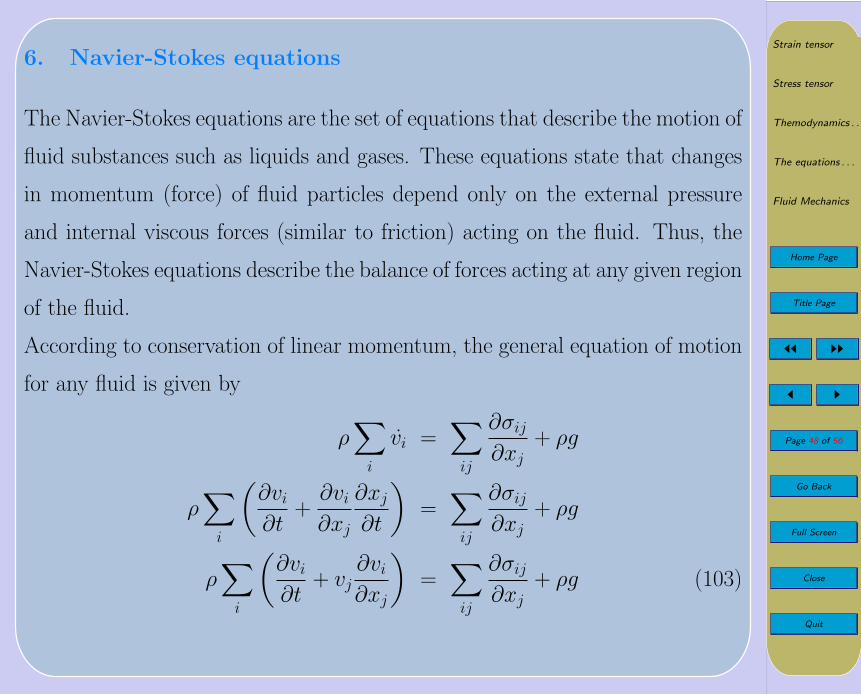
6. Navier-Stokes equations
The Navier-Stokes equations are the set of equations that describe the motion of
fluid substances such as liquids and gases. These equations state that changes
in momentum (force) of fluid particles depend only on the external pressure
and internal viscous forces (similar to friction) acting on the fluid. Thus, the
Navier-Stokes equations describe the balance of forces acting at any given region
of the fluid.
According to conservation of linear momentum, the general equation of motion
for any fluid is given by
ρ∑i
vi =∑ij
∂σij∂xj
+ ρg
ρ∑i
(∂vi∂t
+∂vi∂xj
∂xj∂t
)=∑ij
∂σij∂xj
+ ρg
ρ∑i
(∂vi∂t
+ vj∂vi∂xj
)=∑ij
∂σij∂xj
+ ρg (103)

Strain tensor
Stress tensor
Themodynamics . . .
The equations . . .
Fluid Mechanics
Home Page
Title Page
JJ II
J I
Page 49 of 56
Go Back
Full Screen
Close
Quit
where σij is the stress tensor and is given by
σij = −Pδij for fluid is at rest (104)
σij = −Pδij + τij for fluid is in motion (105)
where P is the force per unit area and τij is called the viscous stress tensor. τij
in terms of rate of strain tensor Dij is given by
τij = 2µ∑l
(Dij −1
3δijDll) +
∑l
ξDll δij refer equation 48(106)
where ξ = (λ + 23µ) is called coefficient of bulk viscosity. λ and µ are the
Lame coefficients. η = µ is called coefficient of shearing viscosity. Then,
σij = −Pδij + τij
σij = −Pδij + 2η∑l
(Dij −1
3δijDll) +
∑l
ξDll ∂ij
∂σij∂xj
= −∂P∂xj
δij + 2η∑l
(∂Dij
∂xj− 1
3δij∂Dll
∂xj
)+∑l
ξ∂Dll
∂xjδij
∂σij∂xj
= −∂P∂xj
+ 2η∑l
(∂Dij
∂xj− 1
3
∂Dll
∂xj
)+∑l
ξ∂Dll
∂xj(107)

Strain tensor
Stress tensor
Themodynamics . . .
The equations . . .
Fluid Mechanics
Home Page
Title Page
JJ II
J I
Page 50 of 56
Go Back
Full Screen
Close
Quit
Substituting for Dij by using equation 102,
∂σij∂xj
= −∂P∂xj
+ η∂2vi∂x2
j
+ η∂2vj∂xi∂xj
− 2η
3
∑l
∂2vl∂xj∂xl
+ ξ∑l
∂2vl∂xj∂xl
(108)
Since,∂2vj∂xi∂xj
=∂2vl∂xj∂xl
equation 108 becomes
∂σij∂xj
= −∂P∂xj
+ η∂2vi∂x2
j
+(ξ +
η
3
) ∂2vj∂xi∂xj
(109)
On substituting equation 109 in equation 103,
ρ∑i
(∂vi∂t
+ vj∂vi∂xj
)= −
∑j
∂P
∂xj+ η
∑ij
∂2vi∂x2
j
+(ξ +
η
3
)∑ij
∂2vj∂xi∂xj
+ ρg
ρ∑i
(∂vi∂t
+ vj.∂
∂xjvj
)= −
∑j
∂P
∂xj+ η
∑i
(∂2
∂x2+∂2
∂y2+∂2
∂z2
)vi
+(ξ +
η
3
)∑ij
∂
∂xi
∂vj∂xj− ρ
∑i
∂Ω
∂xi

Strain tensor
Stress tensor
Themodynamics . . .
The equations . . .
Fluid Mechanics
Home Page
Title Page
JJ II
J I
Page 51 of 56
Go Back
Full Screen
Close
Quit
where Ω is the conservative body force potential given by g = −∇Ω.
ρ
[∂~v
∂t+ (~v.∇)~v
]= −
∑j
∂P
∂xj+ η
∑i
∇2vi +(ξ +
η
3
)∑i
∂
∂xi(∇.~v)− ρ
∑i
∂Ω
∂xi
∂~v
∂t+ (~v.∇)~v = −1
ρ∇P +
η
ρ∇2~v +
1
ρ
(ξ +
η
3
)∇(∇.~v)−∇Ω
∂~v
∂t+ (~v.grad)~v = −1
ρgradP +
η
ρ4~v +
1
ρ
(ξ +
η
3
)grad(∇.~v)−∇Ω (110)
The equation 110 is called Navier-Stokes’ equation. For incompressible fluid
εii = ε11 + ε22 + ε33 = 0 (111)∫Dii =
∫∂vi∂xi
=
∫∇.~v = 0 (112)
That is, if fluid is incompressible, ∇.~v = 0, then the equation 110 becomes
∂~v
∂t+ (∇.~v)~v = −1
ρ∇P +
η
ρ∇2~v −∇Ω (113)
The equation 113 gives Navier-Stokes’ equation for incompressible fluids.

Strain tensor
Stress tensor
Themodynamics . . .
The equations . . .
Fluid Mechanics
Home Page
Title Page
JJ II
J I
Page 52 of 56
Go Back
Full Screen
Close
Quit
7. Flow through a cylindrical pipe: The Poiseuille formula
The rate at which an incompressible viscous fluid flows through a cylindrical
pipe can be calculated from the Navier-Stokes equation. The result is called
Poiseuille’s Law.
Let us consider the velocity field to be zero at the boundaries, where it touches
the walls of the pipe. Just inside the boundary, the steady state velocity to be
same, all the way around the circumference. That is the velocity field to have
circular symmetry, with surfaces of equal velocity being cylinders parallel to the
axis of the pipe.
The Navier-stokes equation for flow of incompressible fluid is given by
∂~v
∂t+ (∇.~v)~v = −1
ρ∇P +
η
ρ∇2~v − g (114)
From the figure it is clear that v = (vx, 0, 0). For a steady state solution,
∂~v
∂t= 0
Since the streamlines have constant velocity, there is no acceleration associated
with change of position of volume element. Therefore (∇.~v)~v = 0. It is assumed

Strain tensor
Stress tensor
Themodynamics . . .
The equations . . .
Fluid Mechanics
Home Page
Title Page
JJ II
J I
Page 53 of 56
Go Back
Full Screen
Close
Quit
that the gravitational effects are small, and set g = 0. Then the equation 114
becomes
− 1
ρ∇P +
η
ρ∇2vx = 0 (115)
In cylindrical coordinates, the equation 115 can be written as
R
~vx
Figure 4: Flow of a viscous fluid in a cylindrical tube.
−(∂P
∂r+
1
r
∂P
∂θ+∂P
∂x
)+ η
[1
r
∂
∂r
(r∂vx∂r
)+
1
r2
∂2vx∂θ2
+∂2vx∂x2
]= 0(116)
The assumption of cylindrical symmetry, plus the assumption that the (symmetry-
breaking) gravitational field is zero, means that our fields must be independent
of the angle θ, so
∂P
∂θ= 0 and
∂vx
∂θ= 0

Strain tensor
Stress tensor
Themodynamics . . .
The equations . . .
Fluid Mechanics
Home Page
Title Page
JJ II
J I
Page 54 of 56
Go Back
Full Screen
Close
Quit
Since, v = (vx, 0, 0) is constant along x direction,
∂vx∂x
= 0 and∂P
∂r= 0
The equation 116, then reduces to
∂P
∂x=
η
r
∂
∂r
(r∂vx∂r
)(117)
For steady flow ∂P∂x = constant = −α (say), then the equation 117 can be
written as
∂
∂r
(r∂vx∂r
)= −αr
η
r∂vx∂r
= −∫αr
ηdr
r∂vx∂r
= −αr2
2η+ a (118)
vx = −∫αr
2ηdr +
∫a
r
vx = −αr2
4η+ a log r + b (119)

Strain tensor
Stress tensor
Themodynamics . . .
The equations . . .
Fluid Mechanics
Home Page
Title Page
JJ II
J I
Page 55 of 56
Go Back
Full Screen
Close
Quit
where a and b are constants, can be evaluated using boundary conditions.
At center of the tube r = 0 and vx is maximum. The equation 118 yields a = 0.
At edge of the tube r = R and vx = 0. The equation 119 yields b = αR2/4η.
Then the equation 119 becomes
vx =α
4η(R2 − r2)dr (120)
If ρ is density of the tube, mass of fluid passes per unit time through an annular
element 2πr dr is ρ 2πr vx dr. Then the flow rate Q, the mass of fluid passes
per unit time through any cross section of the tube (called the discharge) is
Q = 2πρ
∫ R
0
rvx dr (121)
On substituting for vx by using equation 120 to 121,
Q =πρα
2η
∫ R
0
(R2r − r3)dr
Q =πραR4
8η(122)
If ∆P is the pressure difference between any two transverse vertical sections

Strain tensor
Stress tensor
Themodynamics . . .
The equations . . .
Fluid Mechanics
Home Page
Title Page
JJ II
J I
Page 56 of 56
Go Back
Full Screen
Close
Quit
separated by a distance l, then
α =∂P
∂x=
∆P
l
The equation 122 becomes
Q =πρR4∆P
8ηl(123)
Equation 123 is called the Poiseuille formula.