...

CONTINUUM THEORY OF MOISTURE MOVEMENT AND SWELL IN EXPANSIVE CLAYS

by

R. Ray Nach1inger Robert L. Lytton

Research Report Number 118-2

Study of Expansive Clays in Roadway Structural Systems

Research Project 3-8-68-118

conducted for

The Texas Highway Department

in cooperation with the U. S. Department of Transportation

Federal Highway Administration Bureau of Public Roads

by the

CENTER FOR HIGHWAY RESEARCH

THE UNIVERSITY OF TEXAS AT AUSTIN

September 1969

The op1n10ns, findings, and conclusions expressed in this publication are those of the authors and not necessarily those of the Bureau of Public Roads.

ii

..

PREFACE

This report is the second in a series of reports from Research Project

3-8-68-118 entitled "Study of Expansive Clays in Roadway Structural Systems."

The report is a theoretical study of the phenomena of expansive clay which is

viewed as a macroscopically continuous material and is treated with the re­

cently developed and mathematically powerful mixture theory of continuum

mechanics. The subject matter is necessarily abstract but is considered

essential to the formation of a firm analytical foundation for future develop­

ments in the project, including the computer programs to be presented in later

reports and the envisioned field and laboratory experiments which are essential

to a thorough understanding of the mechanics of expansive clay.

The theory of mixtures was devised for studying the properties of mate­

rials with different constituents. Clay is a mixture composed of clay min­

eral, water, and a gas which is itself a mixture of air and water vapor. The

theory of mixtures uses gross mechanical properties of mixtures such as bulk

compressibility rather than trying to deal with the properties of particles

and minerals. The theory of mixtures looks at soil as a continuous material

just as the engineer regards a steel beam as being continuous rather than as

being composed of a collection of randomly connected grains and flakes of iron

and carbon. Modulus of elasticity and Poisson's ratio are sufficient data for

the engineer to make rather accurate computations on the deflections of beams.

The theory of mixtures has been used in this report to obtain a set of

simultaneous nonlinear differential equations which represent the clay mixture.

One of the more significant results of obtaining these equations has been in

identifying the material functions needed to describe the behavior of expansive

clay and in outlining laboratory tests needed to determine these material

functions. Shear modulus, bulk modulus, and permeability are some of the

material functions required, and they are termed "functions" because they are

dependent on water content.

iii

This project is a part of the cooperative highway research program of

the Center for Highway Research, The University of Texas at Austin, and the

Texas Highway Department in cooperation with the U. S. Department of Trans­

portation, Bureau of Public Roads. The Texas Highway Department contact

representative is Larry J. Buttler.

December 1968

R. Ray Nach1inger Robert L. Lytton

iv

,-

"

LIST OF REPORTS

Report No. 118-1, "Theory of Moisture Movement in Expansive Clay" by Robert L. Lytton, presents a theoretical discussion of moisture movement in clay soil.

Report No. 118-2, "Continuum Theory of Moisture Movement and Swell in Expansive Clays" by R. Ray Nach1inger and Robert L. Lytton, presents a theoretical study of the phenomena of expansive clay.

v

,"

ABSTRACT

This report presents a theoretical study of the phenomenon of expansive

clay using the mixture theory of continuum mechanics. The laws concerning

the balance of energy, mass, momentum, and angular momentum are written

together with the general form of constitutive relations. Restrictions on

the independent variables and explicit assumptions about the nature of the

swelling clay phenomenon are applied to the balance laws and constitutive

equations to give some simple, coupled, nonlinear differential equations.

Two coupled equations are required in the isothermal case and three are

required in the nonisotherma1 case.

In considering the isothermal case, it is found that six material func­

tions are required to describe the behavior of the soil under these conditions.

These six functions may be determined using a series of four experiments which

are outlined in this report. An alternate set of four experiments is also

described.

Boundary conditions are discussed and some remarks are made on one­

dimensional problems. The differential equations for nonisotherma1 conditions

are presented and it is shown that 13 material functions are required to

describe the behavior of soil under these conditions.

KEY WORDS: soil mechanics, engineering mechanics, permeability, pore water

pressure, mixtures, constitutive equations, derivation, theoretical (soil)

mechanics, water, soil suction, soil science.

vi

"

TABLE OF CONTENTS

PREFACE • . . • iii

LIST OF REPORTS v

ABSTRACT vi

PARTIAL LIST OF SYMBOLS .• viii

CHAPTER 1. INTRODUCTION

CHAPTER 2. DEVELOPMENT OF THE EQUATIONS FOR MOISTURE MOVEMENT AND SWELL IN SOILS

Notation and Kinematics Balance Laws Constitutive Equations • • • • • • • • ••• An Isotropic Theory of Small Deformations of a Mixture of

Soil, Air, and Water ••••••••••••••

CHAPTER 3. A DISCUSSION OF THE PHYSICAL MEANING OF THE SYSTEM OF EQUATIONS

Ramifications of the Continuum Assumption •••.•••• The Field Equations for Small Deformations and Velocities A Simpler Constitutive Equation for the Isothermal Case Relation to Existing Theories •••• • • • • • • • • • •

CHAPTER 4. A DISCUSSION OF EXPERIMENTS THAT WILL DETERMINE THE CONSTITUTIVE PARAMETERS • . • . • • • • • • • •

CHAPTER 5. ON THE BOUNDARY VALUE PROBLEMS

Boundary and Initial Conditions The Nonisotherma1 Case • • • • •

CHAPTER 6. CONCLUSIONS • • . • . . • •

REFERENCES

vii

. . . . . . . . . . . . . . .

. . . . . . . . . . . . . . .

1

3 5 7

9

12 13 15 16

18

29 31

33

35

Symbol

b ct

E

E*

F ct

g

G

h

H

L

P

,.. P

ct

q

s

T

T ct

u ct

u

v ct

,.. W

ct

PARTIAL LIS T OF SYMBOLS

Body force on the th

ct

Definition

constituent

Infinitesimal strain tensor

Deviatoric strain

Deformation gradient, i.e., measure of the deformation

Grad e

Gas

Heat supply of the mixture

F - I

Liquid

Rate of mass supply

A point in the mixture

Momentum supply

Heat flux of the mixture

Soil

Total stress

Stress on the th ct constituent

Diffusion velocity

Displacement vector

Velocity of the th

ct constituent

Supply of angular momentum

viii

.-

Symbol

x

x

X a

th a

e

p

p* a

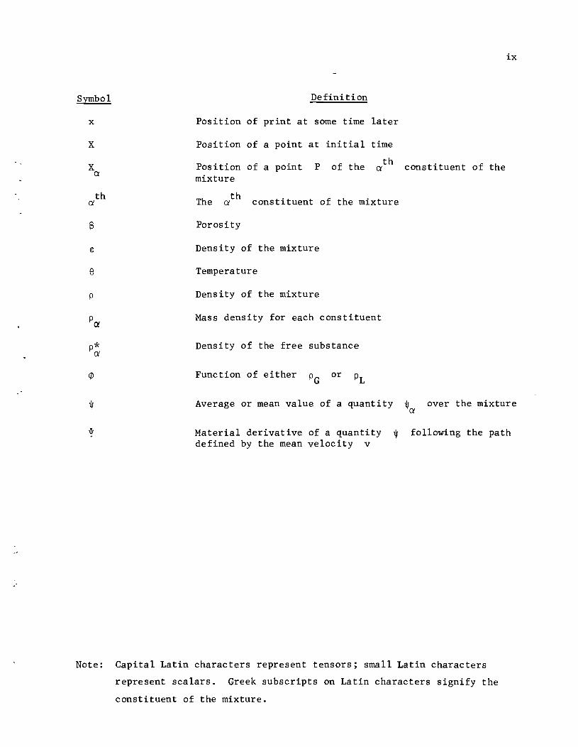
Definition

Position of print at some time later

Position of a point at initial time

Position of a point mixture

P of the th a constituent of the

The th a constituent of the mixture

Porosity

Density of the mixture

Temperature

Density of the mixture

Mass density for each constituent

Density of the free substance

Function of either or

ix

Average or mean value of a quantity ~a over the mixture

Material derivative of a quantity ~ following the path defined by the mean velocity v

Note: Capital Latin characters represent tensors; small Latin characters

represent scalars. Greek subscripts on Latin characters signify the

constituent of the mixture.

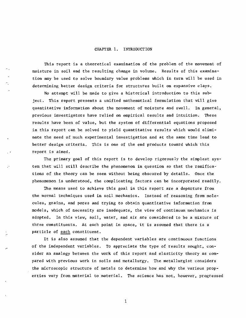
CHAPTER 1. INTRODUCTION

This report is a theoretical examination of the problem of the movement of

moisture in soil and the resulting change in volume. Results of this examina­

tion may be used to solve boundary value problems which in turn will be used in

determining better design criteria for structures built on expansive clays.

No attempt will be made to give a historical introduction to this sub­

ject. This report presents a unified mathematical formulation that will give

quantitative information about the movement of moisture and swell. In general,

previous investigators have relied on empirical results and intuition. These

results have been of value, but the system of differential equations proposed

in this report can be solved to yield quantitative results which would elimi­

nate the need of much experimental investigation and at the same time lead to

better design criteria. This is one of the end products toward which this

report is aimed.

The primary goal of this report is to develop rigorously the simplest sys­

tem that will still describe the phenomenon in question so that the ramifica­

tions of the theory can be seen without being obscured by details. Once the

phenomenon is understood, the complicating factors can be incorporated readily.

The means used to achieve this goal in this report are a departure from

the normal techniques used in soil mechanics. Instead of reasoning from mole­

cules, grains, and pores and trying to obtain quantitative information from

models, which of necessity are inadequate, the view of continuum mechanics is

adopted. In this view, soil, water, and air are considered to be a mixture of

three constituents. At each point in space, it is assumed that there is a

particle of each constituent.

It is also assumed that the dependent variables are continuous functions

of the independent variables. To appreciate the type of results sought, con­

sider an analogy between the work of this report and elasticity theory as com­

pared with previous work in soils and metallurgy. The metallurgist considers

the microscopic structure of metals to determine how and why the various prop­

erties vary from material to material. The science has not, however, progressed

1

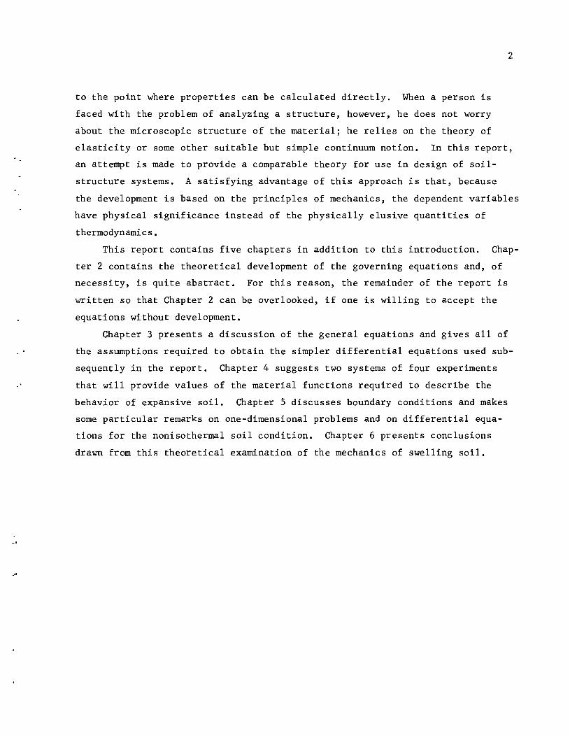
2

to the point where properties can be calculated directly. When a person is

faced with the problem of analyzing a structure, however, he does not worry

about the microscopic structure of the material; he relies on the theory of

elasticity or some other suitable but simple continuum notion. In this report,

an attempt is made to provide a comparable theory for use in design of soil­

structure systems. A satisfying advantage of this approach is that, because

the development is based on the principles of mechanics, the dependent variables

have physical significance instead of the physically elusive quantities of

thermodynamics.

This report contains five chapters in addition to this introduction. Chap­

ter 2 contains the theoretical development of the governing equations and, of

necessity, is quite abstract. For this reason, the remainder of the report is

written so that Chapter 2 can be overlooked, if one is willing to accept the

equations without development.

Chapter 3 presents a discussion of the general equations and gives all of

the assumptions required to obtain the simpler differential equations used sub­

sequently in the report. Chapter 4 suggests two systems of four experiments

that will provide values of the material functions required to describe the

behavior of expansive soil. Chapter 5 discusses boundary conditions and makes

some particular remarks on one-dimensional problems and on differential equa­

tions for the nonisothermal soil condition. Chapter 6 presents conclusions

drawn from this theoretical examination of the mechanics of swelling soil.

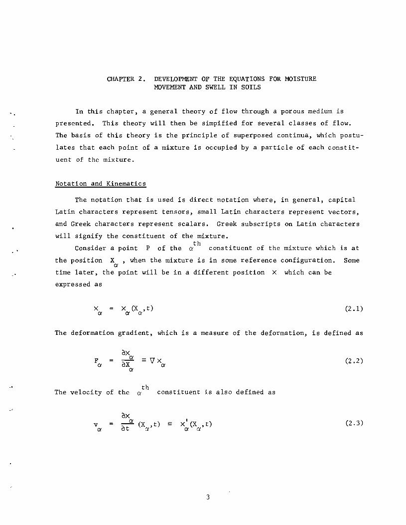
CHAPTER 2. DEVELOPMENT OF THE EQUATIONS FOR MOISTURE MOVEMENT AND SWELL IN SOILS

In this chapter, a general theory of flow through a porous medium is

presented. This theory will then be simpified for several classes of flow.

The basis of this theory is the principle of superposed continua, which postu­

lates that each point of a mixture is occupied by a particle of each constit­

uent of the mixture.

Notation and Kinematics

The notation that is used is direct notation where, in general, capital

Latin characters represent tensors, small Latin characters represent vectors,

and Greek characters represent scalars. Greek subscripts on Latin characters

will signify the constituent of the mixture. th

Consider a point P of the a constituent of the mixture which is at

the position X ,when the mixture is in some reference configuration. Some Ct

time later, the point will be in a different position X which can be

expressed as

X = X (X , t) Ct Ct a

(2.1)

The deformation gradient, which is a measure of the deformation, is defined as

F = Ct

oX ~ aX

Ct

= 'V X Ct

The velocity of the th

constituent is also defined as a

v Ct

= oX ~ (X ,t) at a

, X (X , t)

Ct a

3

(2.2)

(2.3)

.'

4

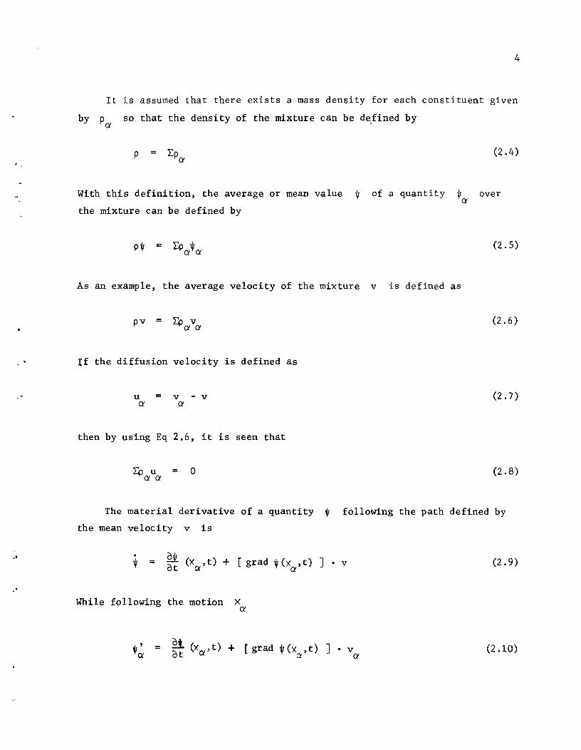
It is assumed that there exists a mass density for each constituent given

by Pa

so that the density of the mixture can be defined by

P =

With this definition, the average or mean value

the mixture can be defined by

=

of a quantity

(2.4)

,I, over fa

(2.5)

As an example, the average velocity of the mixture v is defined as

If the diffusion velocity is defined as

u a

= v - v a

then by using Eq 2.6, it is seen that

= o

(2.6)

(2.7)

(2.8)

The material derivative of a quantity $ following the path defined by

the mean velocity v is

While following the motion X a

$ , Ct

= M. (x ,t ) + [gr ad V (X ,t ) ] • at Ct a v a

(2.9)

(2.10)

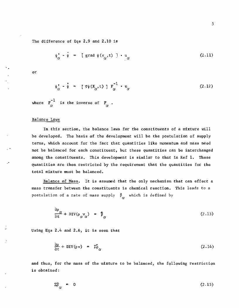
The difference of Eqs 2.9 and 2.10 is

or

where -1

F a

*' - ~ = (grad * (X , t) J • u a a a

•

*' -* a =

is the inverse of F a

• u a

Balance Laws

5

(2.11)

(2.12 )

In this section, the balance laws for the constituents of a mixture will

be developed. The basis of the development will be the postulation of supply

terms, which account for the fact that quantities like momentum and mass need

not be balanced for each constituent, but these quantities can be interchanged

among the constituents. This development is similar to that in Ref 1. These

quantities are then restricted by the requirement that the quantities for the

total mixture must be balanced.

Balance of Mass. It is assumed that the only mechanism that can effect a

mass transfer between the constituents is chemical reaction. This leads to a

postulation of a rate of mass supply Pa

which is defined by

op ~ + DIV(p v ) at a a

= (2.13)

Using Eqs 2.4 and 2.6, it is seen that

~ + DIV(pv) (2.14 )

and thus, for the mass of the mixture to be balanced, the following restriction

is obtained:

o (2.15 )

,"

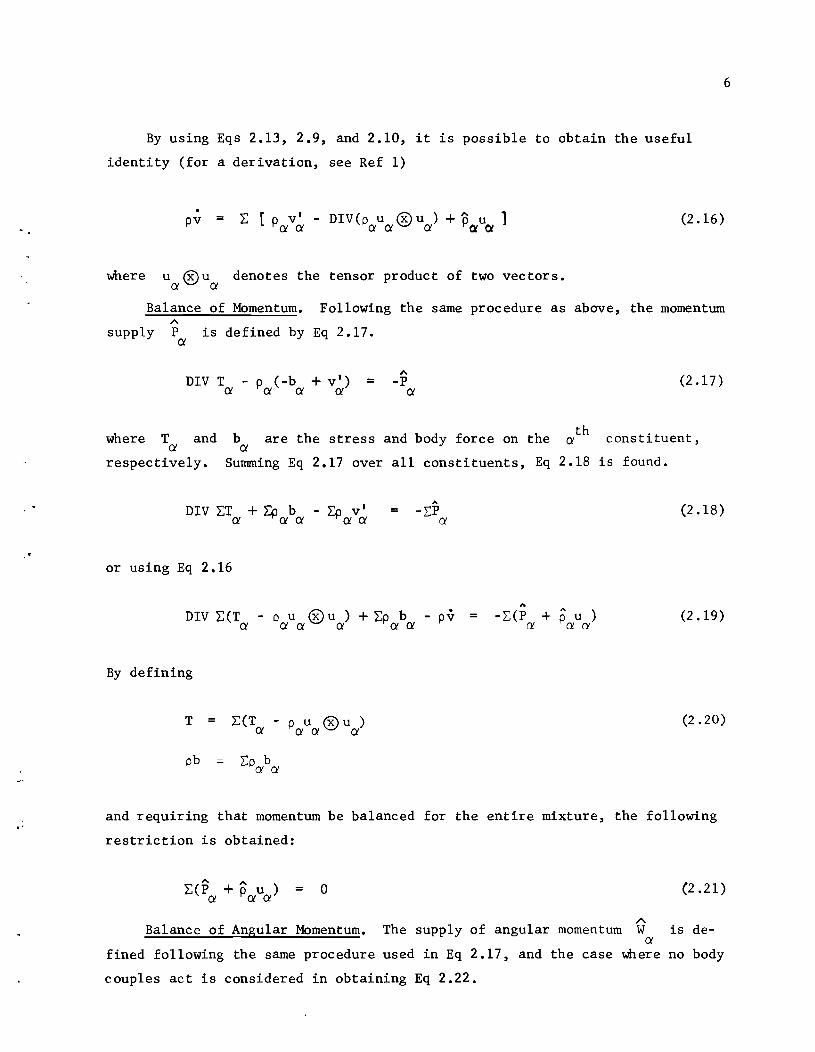
By using Eqs 2.13, 2.9, and 2.10, it is possible to obtain the useful

identity (for a derivation, see Ref 1)

pv = l: [ p v' - DIV(p u ® u ) + P u 1 a a a a a 0/ 0/

where u ®u denotes the tensor product of two vectors. a a

(2.16)

6

Balance of Momentum. Following the same procedure as above, the momentum

supply A

P a

is defined by Eq 2.17.

DIV T - P (-b + v') = a a a a

'" -P a

where T and a

b a

are the stress and body force on the th a

(2.17)

constituent,

respectively. Summing Eq 2.17 over all constituents, Eq 2.18 is found.

DIV l:T + l:p b - l:p v' = -2:P a aa aa a

or using Eq 2.16

,. DIV l:(T - 0 u ®u ) + l:p b - pv = -2:(P + P u )

a a a a a a a Li Li

By defining

T = L:(T - P u ® u ) a a a a

pb 2:p b aa

(2.18)

(2.19)

(2.20)

and requiring that momentum be balanced for the entire mixture, the following

restriction is obtained:

,.. ,.. l:(P + P u) = 0 a a a

(2.21 )

'" Balance of Angular Momentum. The supply of angular momentum W is de-a

fined following the same procedure used in Eq 2.17, and the case where no body

couples act is considered in obtaining Eq 2.22.

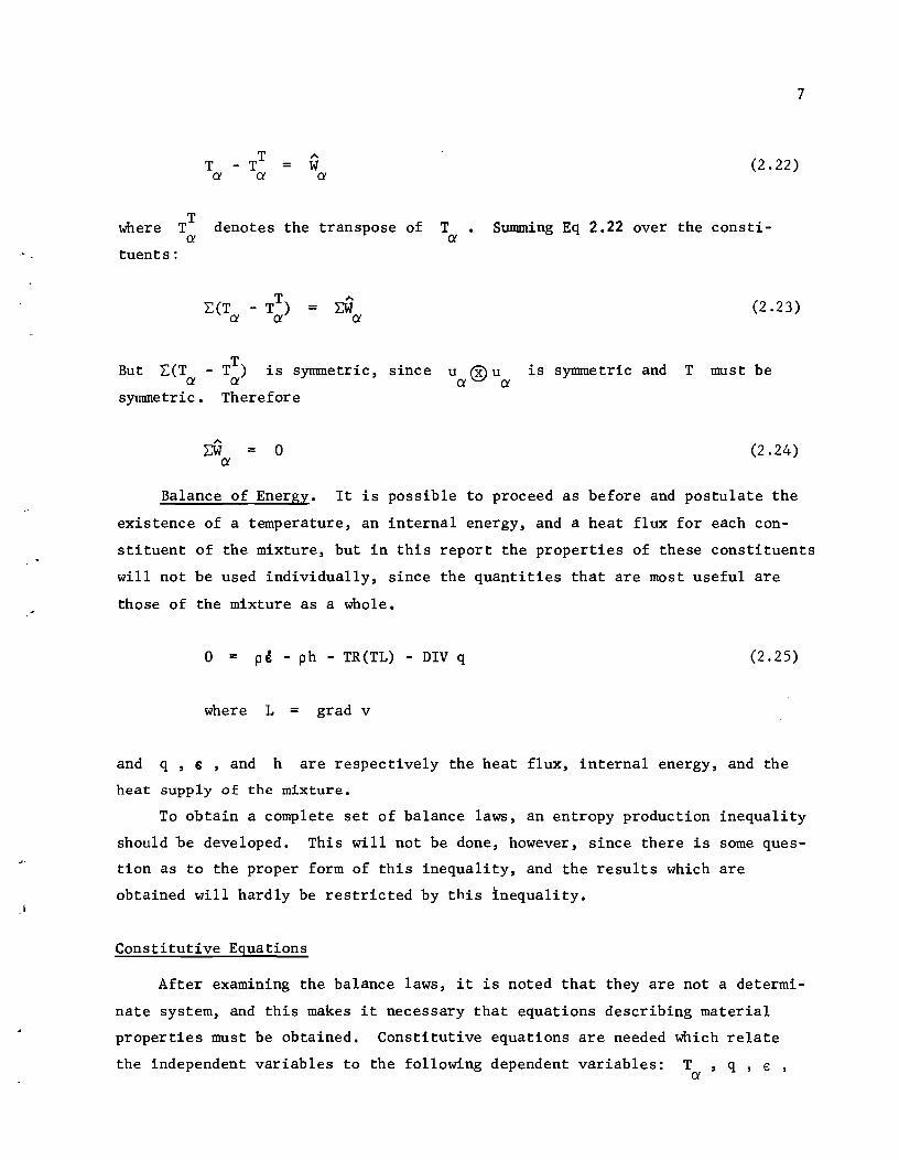
T ex =

7

(2.22 )

where TT ex

denotes the transpose of T ex

Summing Eq 2.22 over the consti-

tuents:

L:(T ex '" = r:w ex

(2.23)

But L:(T - TT) is syrranetric, since u ® u is synnnetric and T must be ex ex ex ex

symmetric. Therefore

'" r:w = 0 ex

(2.24)

Balance of Energy. It is possible to proceed as before and postulate the

existence of a temperature, an internal energy, and a heat flux for each con­

stituent of the mixture, but in this report the properties of these constituents

will not be used individually, since the quantities that are most useful are

those of the mixture as a whole.

o = pe - ph - TR(TL) - DIV q (2.25)

where L = grad v

and q, £ , and h are respectively the heat flux, internal energy, and the

heat supply of the mixture.

To obtain a complete set of balance laws, an entropy production inequality

should be developed. This will not be done, however, since there is some ques­

tion as to the proper form of this inequality, and the results which are

obtained will hardly be restricted by this inequality.

Constitutive Equations

After examining the balance laws, it is noted that they are not a determi­

nate system, and this makes it necessary that equations describing material

properties must be obtained. Constitutive equations are needed which relate

the independent variables to the following dependent variables: T ,q, € , ex

.'

8

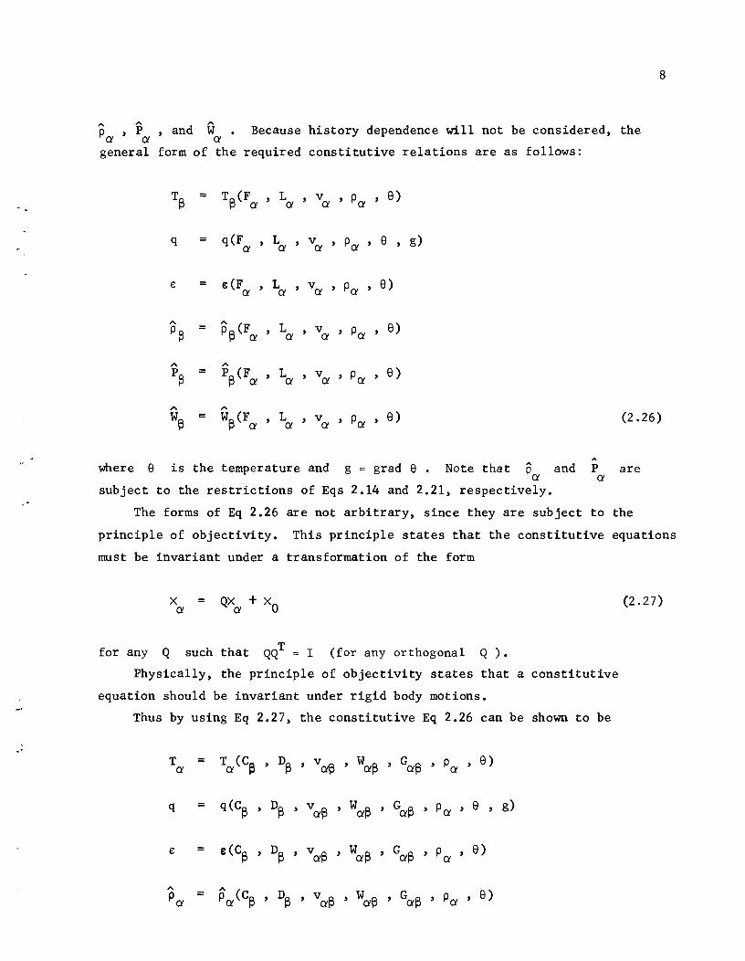
p ,P ,and W Because history dependence will not be considered, the a a a

general form of the required constitutive relations are as follows:

T~ = T~(Fa L v P ,e) a a a

q = q(F L v Pa ' e g) a a a

,

EO = e(F L v Pa ' e) a a a

" p ~ (Fa L Pa ' e) P~ = v a a

" " P~ = P~(Fa L v Pa ' e) a a

" A

W~ = W~(Fa L v ,Pa,e) (2.26 ) a a

A

where e is the temperature and g = grad e • Note that A and P Pa are

a subject to the restrictions of Eqs 2.14 and 2.21, respectively.

The forms of Eq 2.26 are not arbitrary, since they are subject to the

principle of objectivity. This principle states that the constitutive equations

must be invariant under a transformation of the form

for any Q such that QQT = I (for any orthogonal Q).

Physically, the principle of objectivity states that a constitutive

equation should be invariant under rigid body motions.

Thus by using Eq 2.27, the constitutive Eq 2.26 can be shown to be

T = Ta(C~ , D~ , va~ , Wa~ , Ga~ P ,e) a a

q = q(C~ D!3 va~ Wa!3 Gal' P a ' e , g)

€ = e(C~ D~ , v a~ , Wa~ Ga~ P ,e) a

" Pa(C~ , D!3 ' va~ , Wa~ , Gal' ' Pa ' e) Pa =

(2.27)

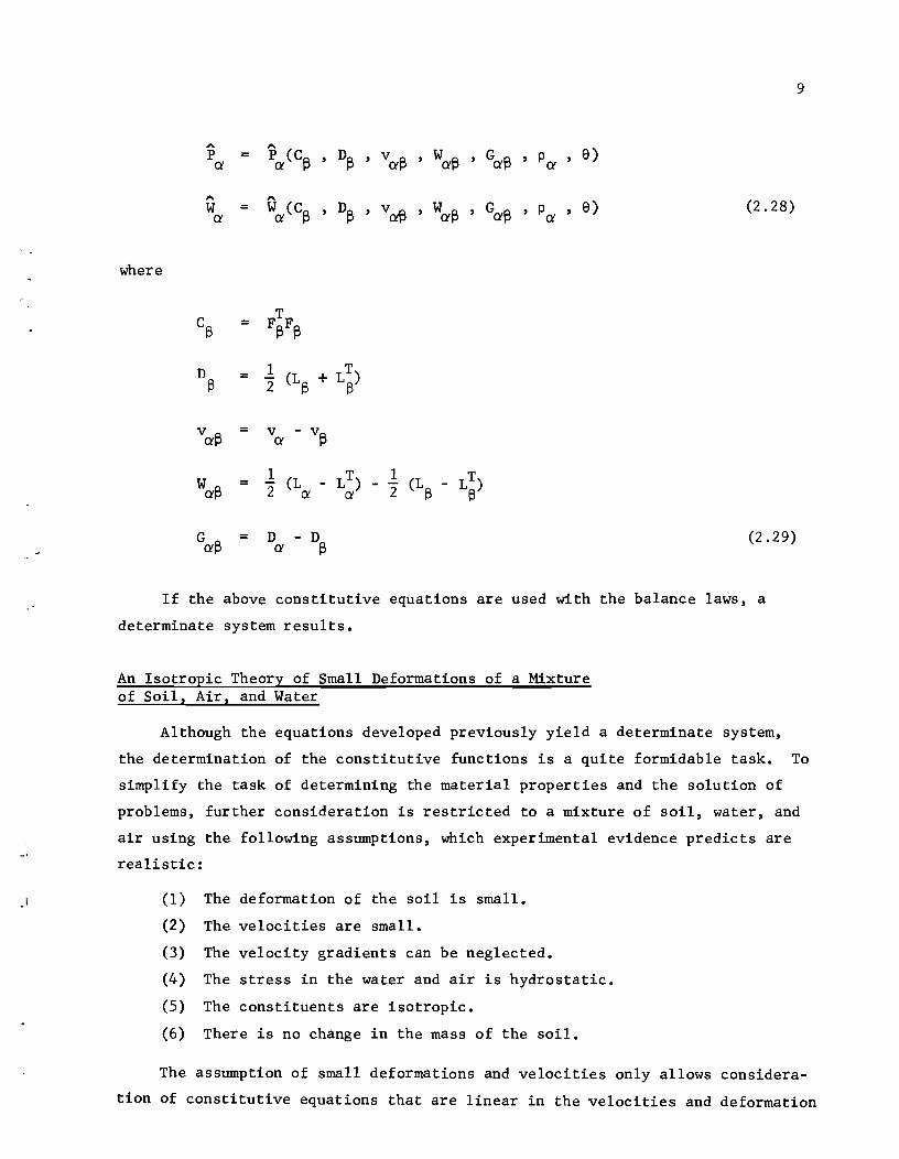
A " , e) p '= PO' (C~ D~ vO'~ WO'~ GO'~ PO' 0'

" " W '= WO'(C~ , D~ , vO'~ , WO'~ , GO'~ , PO' ' e) 0'

(2.28)

where

eS

T = F~F~

D = 1 (LS + LT)

~ 2 S

vO'~ = V - V 0' ~

WO'~ 1

(L - LT) 1 (L - LT) = 2 Ci Ci 2 S e

GO'~ = D 0' D~ (2.29)

If the above constitutive equations are used with the balance laws, a

determinate system results.

An Isotropic Theory of Small Deformations of a Mixture of Soil. Air. and Water

9

Although the equations developed previously yield a determinate system,

the determination of the constitutive functions is a quite formidable task. To

simplify the task of determining the material properties and the solution of

problems, further consideration is restricted to a mixture of soil, water, and

air using the following assumptions, which experimental evidence predicts are

realistic:

(1) The deformation of the soil is small.

(2) The velocities are small.

(3) The velocity gradients can be neglected.

(4) The stress in the water and air is hydrostatic.

(5) The constituents are isotropic.

(6) There is no change in the mass of the soil.

The assumption of small deformations and velocities only allows considera­

tion of constitutive equations that are linear in the velocities and deformation

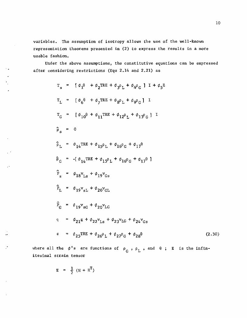
variables. The assumption of isotropy allows the use of the well-known

representation theorems presented in (2) to express the results in a more

usable fashion.

10

Under the above assumptions, the constitutive equations can be expressed

after considering restrictions (Eqs 2.14 and 2.21) as

T = ( ¢19 + ¢2TRE + ¢3PL + ¢4PG ] I + ¢SE s

TL = ( ¢69 + ¢ 7 TRE + ¢ 8P L + ¢ 9P G 1 I

TG = [ ¢109 + ¢ 11 TRE + ¢ 12P L + ¢ 13P G 1 I

" 0 Ps =

" ¢14TRE + ¢lSPL + ¢16PG + ¢179 PL =

" = -( ¢14TRE + ¢lSP L + ¢16PG + ¢179 1 PG

A

P = ¢18vLs + ¢19vGs s

A

PL = ¢19 v sL + ¢20vGL

" PG = ¢19v sG + ¢20vLG

q =

(2.30)

where all the ¢IS are functions of P G ' PL ' and 9 E is the infin-

itesimal strain tensor

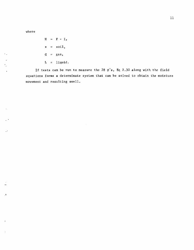
11

where

H == F - I,

s == soil,

G gas,

L liquid.

If tests can be run to measure the 28 ¢'s, Eq 2.30 along with the field

equations forms a determinate system that can be solved to obtain the moisture

movement and resulting swell.

CHAPTER 3. A DISCUSSION OF THE PHYSICAL MEANING OF THE SYSTEM OF EQUATIONS

In Chapter 2, a system of equations for describing the movement of water

and the resulting swell was derived from the principles of continuum mechanics.

This marks a distinct departure from the present way of considering the prob­

lem. To make the difference clearer, the physical interpretation of the assump­

tions that were made will be considered in this chapter together with the

physical interpretation of the equations.

Ramifications of the Continuum Assumption

The two basic assumptions in mixture continuum mechanics are that the de­

pendent variables depend continuously on the independent variables and that par­

ticles of each constituent exist at every point in the body. On a microscopic

scale, it is obvious that these assumptions are not satisfied by a mixture of

soil, water, and air. The question thus comes to mind as to whether or not

this inconsistency makes useless the equations that were derived from mixture

continuum theory. The answer to this question is that these equations are

quite useful.

The reason that they are useful is that the phenomenon of interest is the

macroscopic one of moisture movement and swell in masses of soil that are very

large in comparison to the dimensions of the pores in which the water moves.

Thus the equations are seen to yield averages of the microscopic quantities

over a region of the material.

Now it becomes obvious that the philosophy of this approach is to replace

the intricate (and intractable) problem of trying to describe how the water

will flow through the pores of a solid with the much simpler problem of trying to

to describe the gross phenomenon. This gives some insight into the physical

meaning of the ¢'s. They are the things that take into account the average

porosity, surface tension, viscosity, etc., and they must be measured on a

gross scale.

12

13

This approach does not deny the importance of work that has been done on

the mechanisms of moisture movement on the microscopic scale. This type work

can predict qualitatively how the phenomenon will vary from material to mate.­

rial. However, to expect this work to give quantitative answers about the gross

phenomenon is to expect too much of nature and of the ingenuity of investiga­

tors. It is always useful to recall the analogy between this work and elas­

ticity. When analyzing a structure, dislocation theory is not used. -Instead,

measured values of the elastic properties are used with the elasticity theory

to obtain an average of the response. The fact that these results rely on mea­

sured properties and do not take into account the motion of microscopic disloca­

tions does not keep the elasticity results from accurately predicting the

phenomenon.

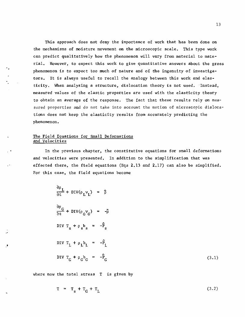
The Field Equations for Small Deformations and Velocities

In the previous chapter, the constitutive equations for small deformations

and velocities were presented. In addition to the simplification that was

effected there, the field equations (Eqs 2.13 and 2.17) can also be simplified.

For this case, the field equations become

aP L DIV(P L vL) " -+ = P at

aP G DIV(PGVG)

A -+ = -P ot

" DIV T + P b = -p s s s S

A

DIV TL + PLbL = -p

L

" DIV TG + PGbG = -p G (3.1)

where now the total stress T is given by

(3.2)

.~

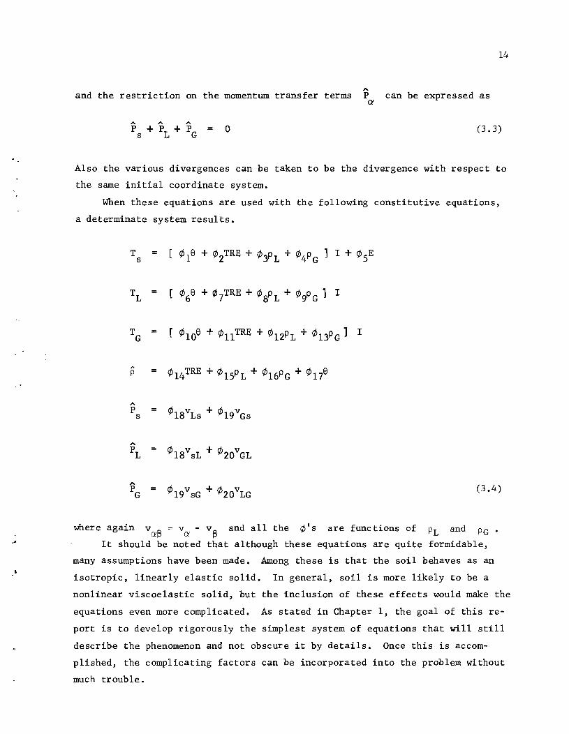
14

" and the restriction on the momentum transfer terms P can be expressed as Ct

= o (3.3)

Also the various divergences can be taken to be the divergence with respect to

the same initial coordinate system.

When these equations are used with the following constitutive equations,

a determinate system results.

TL = [ ¢69 + ¢7TRE + ¢SP L + ¢9P G 1 I

TG = [ ¢ 109 + ¢1l TRE + ¢12PL + ¢13P G ] I

" = ¢14TRE + ¢lSP L + ¢16PG + ¢179 P

A

P = ¢lSvLs + ¢19vGs s

" PL = ¢lSvsL + ¢20vGL

" (3.4) PG = ¢19v sG + ¢20vLG

where again vaS = va - Vs and all the ¢'s are functions of PL and PG'

It should be noted that although these equations are quite formidable,

many assumptions have been made. Among these is that the soil behaves as an

isotropic, linearly elastic solid. In general, soil is more likely to be a

nonlinear viscoelastic solid, but the inclusion of these effects would make the

equations even more complicated. As stated in Chapter 1, the goal of this re­

port is to develop rigorously the simplest system of equations that will still

describe the phenomenon and not obscure it by details. Once this is accom­

plished, the complicating factors can be incorporated into the problem without

much trouble.

15

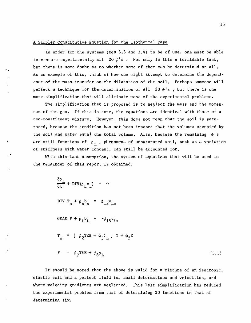
A Simpler Constitutive Equation for the Isothermal Case

In order for the systems (Eqs 3.3 and 3.4) to be of use, one must be able

to measure experimentally all 20 ¢IS. Not only is this a formidable task,

but there is some doubt as to whether some of them can be determined at all.

As an example of this, think of how one might attempt to determine the depend­

ence of the mass transfer on the dilatation of the soil. Perhaps someone will

perfect a technique for the determination of all 20 ¢IS , but there is one

more simplification that will eliminate most of the experimental problems.

The simplification that is proposed is to neglect the mass and the momen­

tum of the gas. If this is done, the equations are identical with those of a

two-constituent mixture. However, this does not mean that the soil is satu­

rated, because the condition has not been imposed that the volumes occupied by

the soil and water equal the total volume. Also, because the remaining ¢IS are still functions of P

L, phenomena of unsaturated soil, such as a variation

of stiffness with water content, can still be accounted for.

With this last assumption, the system of equations that will be used in

the remainder of this report is obtained:

DIV T + P b s s s

T s

p

=

= o

=

(3.5)

It should be noted that the above is valid for a mixture of an isotropic,

elastic soil and a perfect fluid for small deformations and velocities, and

where velocity gradients are neglected. This last simplification has reduced

the experimental problem from that of determining 20 functions to that of

determining six.

16

Relation to Existing Theories

To make comparisons of the system, Eq 3.5, with existing theories, the

only body force is taken to be gravity and the velocity of the soil is assumed

to be zero. Also, a new parameter K is defined and the following relations

are written:

= GRAD Y Z s

Equations 3.5 can now be written

where

Of)

K GRAD H =

DIV

H

+ GRAD(y Z + H) = 0 s

Note that the second of Eqs 3.7 is the well-known Darcy's Law.

(3.6)

(3.7)

If the first two equations are combined, the well-known flow or diffusion

equation is obtained.

Of)

at - DIV(K GRAD H) = 0 (3.8)

17

This equation cannot be solved alone, however, because it is coupled to the

balance of momentum for the solid through H. Also, by observing the second

equation, one would be tempted to say that the presence of the liquid affects

the solid like a body force which is the gradient of the head causing flow

H. This is not, in general, true, since the liquid also affects the stress

in the solid through the constitutive equation as well as through the balance

laws. Thus, these results show that that Eq 3.6 can be put into a form that is

similar to that now used, but the interpretation of the terms is different from

that which has been used previously.

CHAPTER 4. A DISCUSS ION OF EXPERIMENTS THAT WILL DETERMINE THE CONSTITUTIVE PARAMETERS

Before any of this work can be of use, the ¢'s must be determined

experimentally. In this chapter, a set of experiments that will determine the

¢'s will be discussed. Although there are infinitely many experiments that

can be run, the prime consideration in the choice of the ones that will be

presented is simplicity. These experiments will require measurements of

quantities such as strain, concentration, and total stress. These measure­

ments can be made with reasonable accuracy and simplicity.

The constitutive equations for isothermal stress conditions given by

Eqs 4.1 contain five functions. Note that the function numbering given here

is, as a matter of convenience, different from that given in Eq 3.4.

=

= (4.1)

In addition, a permeability function defined by Eq 4.2 is to be determined.

= (4.2)

Thus, there is a total of six functions of the density of the fluid to be deter­

mined. This will require a series of four tests, all four performed for vari­

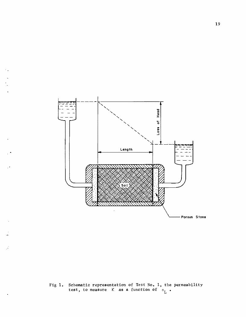
ous values of PL' A graphic description of five experiments which can be

used is found in Figs 1 through 5. The following discussion indicates how these

tests may be used.

If Eq 4.2 is rewritten using

18

I ----.:::-- _. - ----"'--------------. .... -- , - - -- , - - _. , "-

"­"-

"-"-

"-"-

Length

"-"­

"­,

-o en .. o ..J

'I ~-

Porous Stone

Fig 1. Schematic representation of Test No.1, the permeability test, to measure K as a function of 0L •

19

50."\ '--f-..... ;,,' .... ,

,If

" /\ I , I ,

I \ , \

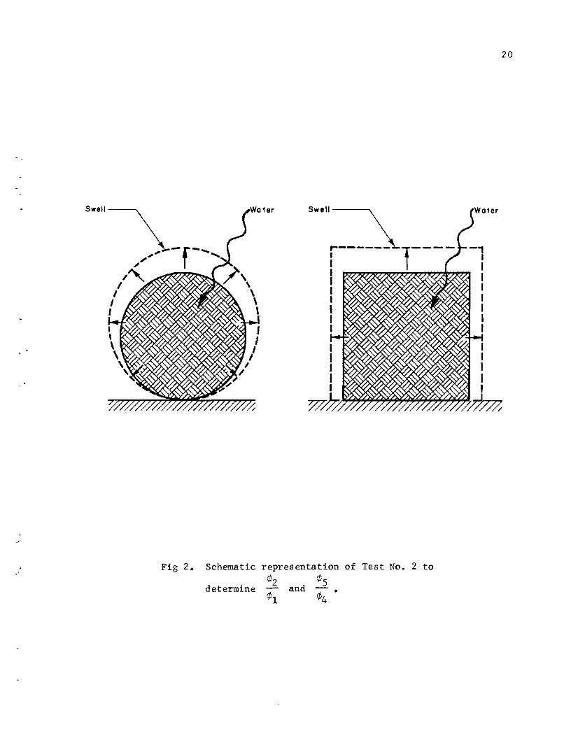
Fig 2. Schematic

determine

swel'~

r-----~r---I I I I I I I

representation of ¢2 ¢S - and -. ¢1 ¢4

Test No.2 to

20

Pressure

Controlled Amount of Water

Porous Stone

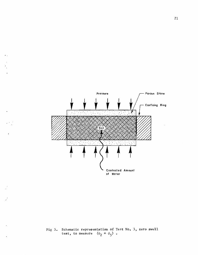
Fig 3. Schematic representation of Test No.3, zero swell test, to measure (¢z + ¢S) •

21

• ,/"",~----- .......... , /" / '\!

I \ I \ I \

I \ I , .. , I \ I \ / \ I

\ /

/" ........... _----;""'/' ~ H,d",f,!;e P .. "",,

.... __ .... t H,d,,","e Pressure

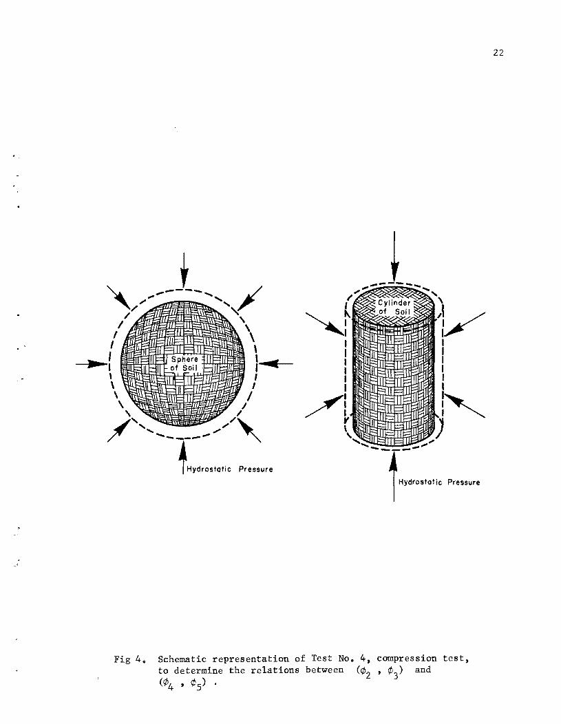
Fig 40 Schematic representation of Test No o 4, compression test, to determine the relations between (¢2' ¢3) and (¢4 ' ¢S) •

22

Shear Force

)III

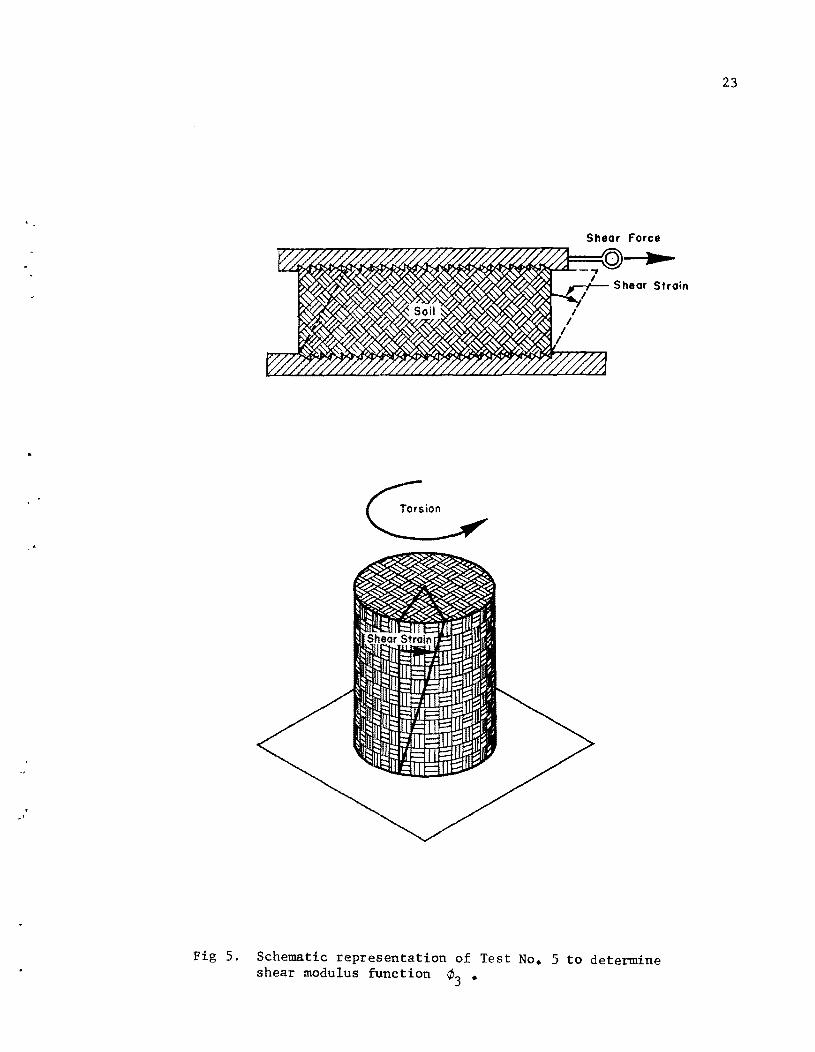
Fig 5. Schematic representation of Test No. 5 to determine shear modulus function ¢3 •

23

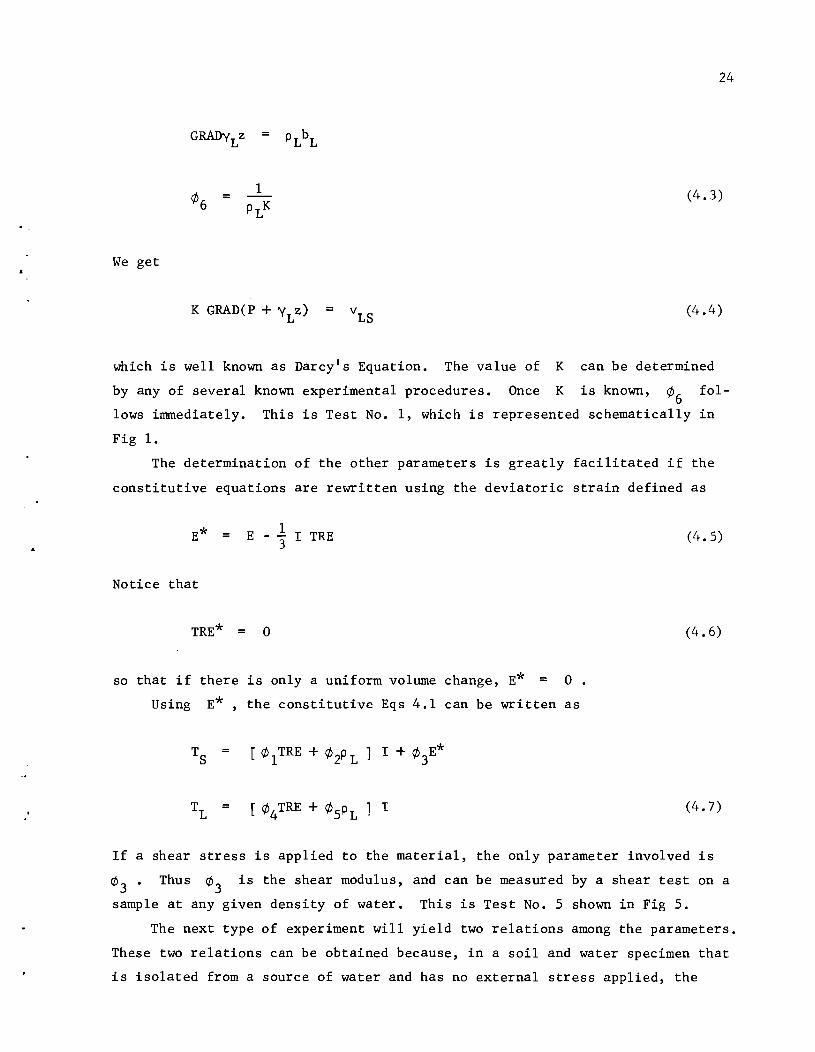
24

=

= (4.3)

We get

= (4.4 )

which is well known as Darcy's Equation. The value of K can be determined

by any of several known experimental procedures. Once K is known, ¢6 fol­

lows immediately. This is Test No.1, which is represented schematically in

Fig 1.

The determination of the other parameters is greatly facilitated if the

constitutive equations are rewritten using the deviatoric strain defined as

E* = E - ~ I TRE (4.5)

Notice that

TRE* = 0 (4.6)

so that if there is only a uniform volume change, E* = O.

Using E*, the constitutive Eqs 4.1 can be written as

= (4.7)

If a shear stress is applied to the material, the only parameter involved is

Thus is the shear modulus, and can be measured by a shear test on a

sample at any given density of water. This is Test No.5 shown in Fig 5.

The next type of experiment will yield two relations among the parameters.

These two relations can be obtained because, in a soil and water specimen that

is isolated from a source of water and has no external stress applied, the

25

external stress in both the water and in the soil is zero. Thus if one starts

with an initially dry spherical sample of soil and adds a known amount of water,

the density of the water is known. If ample time is allowed for the water to

move throughout the specimen, symmetry requires E* to be zero and the change

in volume is easily measured, so that E*, TRE , PL ' TL ' and TS are all

known. This is Test No.2 shown in Fig 2 and it gives two relations among the

remaining four unknown parameters.

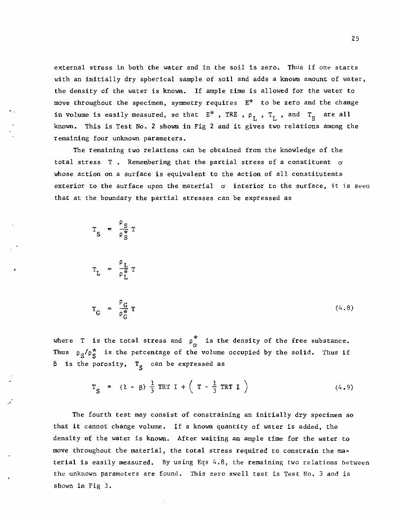
The remaining two relations can be obtained from the knowledge of the

total stress T. Remembering that the partial stress of a constituent a

whose action on a surface is equivalent to the action of all constitutents

exterior to the surface upon the material a interior to the surface, it is seen

that at the boundary the partial stresses can be expressed as

~&e

Thus

T S

=

=

=

Ps -T p*

S

PL -T p*

L

PG -T p*

G (4.8)

* T is the total stress and Pa

is the density of the free substance.

PS/p; is the percentage of the volume occupied by the solid. Thus if

~ is the porosity, TS can be expressed as

(1 - ~) ~ TRT I + ( T - 1 TRT I ) (4.9)

The fourth test may consist of constraining an initially dry specimen so

that it cannot change volume. If a known quantity of water is added, the

density of the water is known. After waiting an ample time for the water to

move throughout the material, the total stress required to constrain the ma­

terial is easily measured. By using Eqs 4.8, the remaining two relations between

the unknown parameters are found. This zero swell test is Test No.3 and is

shown in Fig 3.

..

26

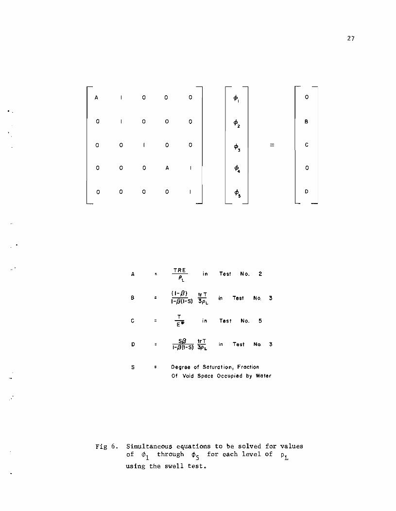
Thus if these tests are performed for various values of the water density,

the material parameters can be easily obtained as a function of the density.

The system of equations derived from these tests is given in Fig 6.

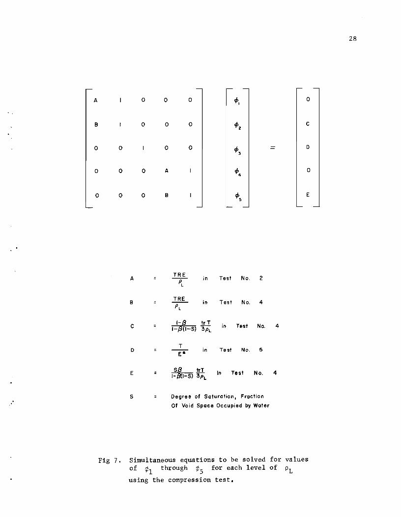
A compression test (Fig 4) may be used in place of the zero volume change

test. In this test, a soil specimen of known water density is subjected to a

known total stress and the volume strain is measured. A different set of

equations is produced and these equations are shown in Fig 7.

A 0 0 0 q,1

0 0 0 0 q,z

0 0 0 0 q,3

0 0 0 A q,4

0 0 0 0 q,S

A TRE

in Test No. 2 = PL

B = ( 1-{3) tr T

in Test No. 3 1-{3(1-5) 3PL

c = T

EW in Test No. 5

D = slJ. trT in Test No. ~ 1-,8(1-5) 3PL

s = Degree of Saturation, Fraction

Of Void Space Occupied by Water

Fig 6. Simultaneous equations to be solved for values of ¢l through ¢s for each level of PL using the swell test.

27

0

B

C

0

D

. .

A 0 0 0 ifJ1 0

B 0 0 0 ifJz c

0 0 0 0 ifJ) D

0 0 0 A ifJ4

0

0 0 0 B ifJS E

A = TRE in Test No. 2

PL

B TRE

in Test No. 4 PL

C I-~ tr T in Test No. 4 1-/81-5) 3PL

T D

E-in Test No. 5

E ~trT 1- 1-5) 3h In Test No. 4

5 Degree of Saturation, Fraction

Of Void Space Occupied by Water

Fig 7. Simultaneous equations to be solved for values of ¢l through ¢s for each level of PL using the compression test.

28

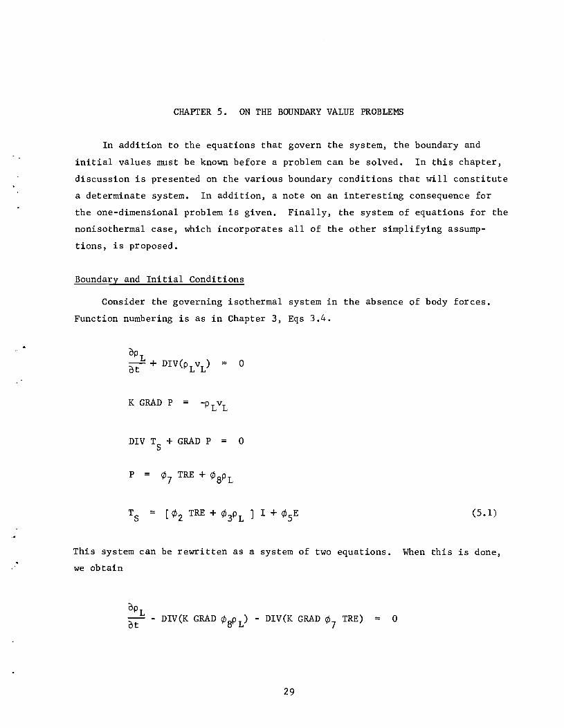
CHAPI'ER 5. ON THE BOUNDARY VALUE PROBLEMS

In addition to the equations that govern the system, the boundary and

initial values must be known before a problem can be solved. In this chapter,

discussion is presented on the various boundary conditions that will constitute

a determinate system. In addition, a note on an interesting consequence for

the one-dimensional problem is given. Finally, the system of equations for the

nonisothermal case, which incorporates all of the other simplifying assump­

tions, is proposed.

Boundary and Initial Conditions

Consider the governing isothermal system in the absence of body forces.

Function numbering is as in Chapter 3, Eqs 3.4.

= o

K GRAD P =

DIV TS + GRAD P = o

= (5.1)

This system can be rewritten as a system of two equations. When this is done,

we obtain

op ot

L - DIV(K GRAD ¢8PL) - DIV(K GRAD ¢7 TRE) = 0

29

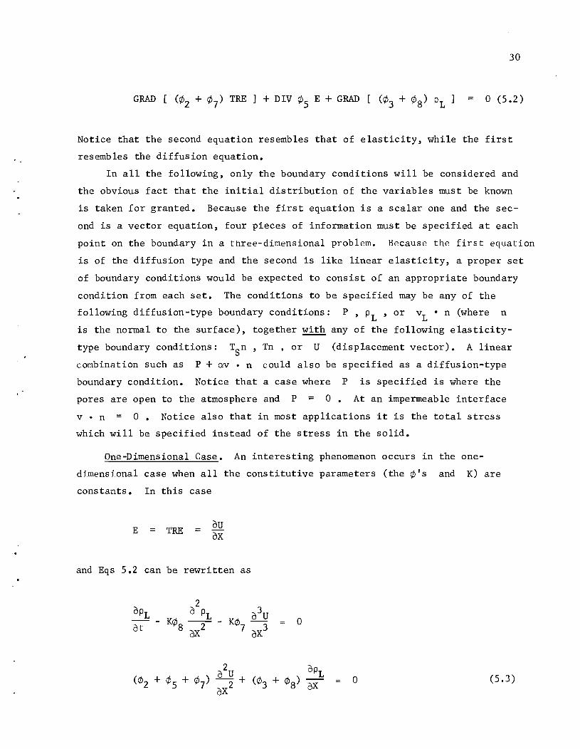
30

Notice that the second equation resembles that of elasticity, while the first

resembles the diffusion equation.

In all the following, only the boundary conditions will be considered and

the obvious fact that the initial distribution of the variables must be known

is taken for granted. Because the first equation is a scalar one and the sec­

ond is a vector equation, four pieces of information must be specified at each

point on the boundary in a three-dimensional problem. Because the first equation

is of the diffusion type and the second is like linear elasticity, a proper set

of boundary conditions would be expected to consist of an appropriate boundary

condition from each set. The conditions to be specified may be any of the

following diffusion-type boundary conditions: P, PL ,or vL • n (where n

is the normal to the surface), together with any of the following elasticity­

type boundary conditions: TSn, Tn , or U (displacement vector). A linear

combination such as P + QV • n could also be specified as a diffusion-type

boundary condition. Notice that a case where P is specified is where the

pores are open to the atmosphere and P = o At an impermeable interface

= o • Notice also that in most applications it is the total stress

which will be specified instead of the stress in the solid.

One-Dimensional Case. An interesting phenomenon occurs in the one­

dimensional case when all the constitutive parameters (the ¢'s and K) are

constants. In this case

E = TRE = aU oX

and Eqs 5.2 can be rewritten as

2 a PL

- K¢ ---8 ox2 o

o (5.3)

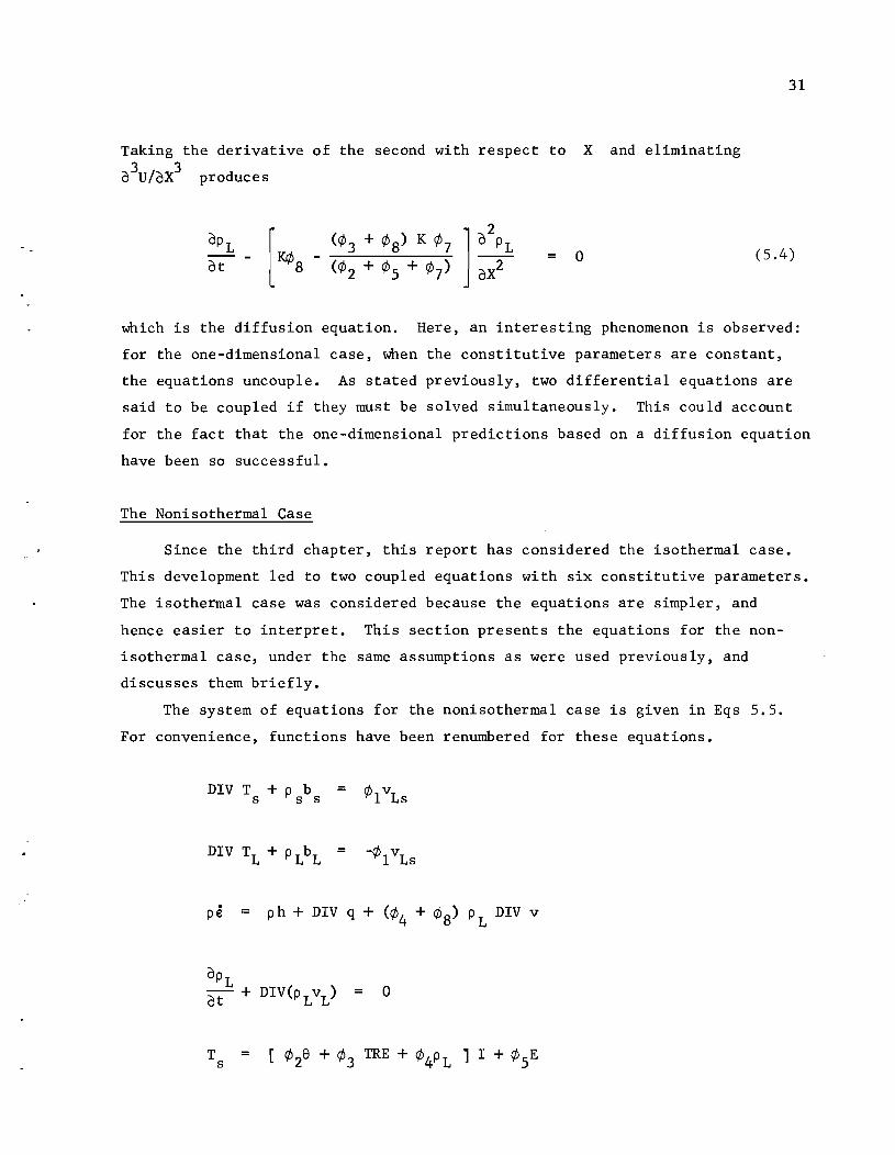
Taking the derivative of the second with respect to X and eliminating

o3u/ oX3 produces

31

(¢3 + ¢S) K ¢7

(¢2 + ¢S + ¢7) = o (5.4)

which is the diffusion equation. Here, an interesting phenomenon is observed:

for the one-dimensional case, when the constitutive parameters are constant,

the equations uncouple. As stated previously, two differential equations are

said to be coupled if they must be solved simultaneously. This could account

for the fact that the one-dimensional predictions based on a diffusion equation

have been so successful.

The Nonisothermal Case

Since the third chapter, this report has considered the isothermal case.

This development led to two coupled equations with six constitutive parameters.

The isothermal case was considered because the equations are simpler, and

hence easier to interpret. This section presents the equations for the non­

isothermal case, under the same assumptions as were used previously, and

discusses them briefly.

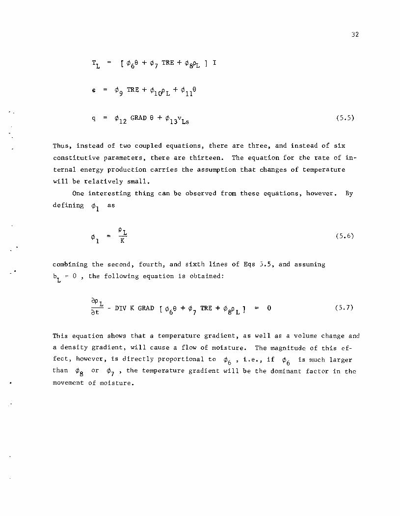
The system of equations for the nonisothermal case is given in Eqs 5.5.

For convenience, functions have been renumbered for these equations.

DIV T + P b s s s =

=

pe =

= o

32

T L [ ¢ 6 e + ¢ 7 TRE + ¢ aPL ] I

q = (5.5)

Thus, instead of two coupled equations, there are three, and instead of six

constitutive parameters, there are thirteen. The equation for the rate of in­

ternal energy production carries the assumption that changes of temperature

will be relatively small.

One interesting thing can be observed from these equations, however. By

defining ¢l as

¢l PL = K

combining the second, fourth, and sixth lines of Eqs 5.5, and assuming

bL

~ 0 , the following equation is obtained:

(5.6)

(5.7)

This equation shows that a temperature gradient, as well as a volume change and

a density gradient, will cause a flow of moisture. The magnitude of this ef­

fect, however, is directly proportional to ¢6 ' i.e., if ¢6 is much larger

than ¢a or ¢7 ' the temperature gradient will be the dominant factor in the

movement of moisture.

CHAPTER 6. CONCLUSIONS

As was stated in the introduction, the goal of this work is the simplest

rigorous formulation of the problem that still describes the phenomenon. The

system, Eq 3.5, appears to achieve this goal. However, the level of mathemati­

cal rigor used in this report needs to be discussed. This work was not planned

to be a contribution to the basic formulation of mixture theory. The main con­

tribution lies not in the development of the balance laws, since they are well

known, but in the constitutive equations and the interpretation of the various

results. Also, because this work was intended for use in soil mechanics, and

in the interest of clarity, some mathematical rigor and precision has purposely

been deleted.

The conspicuous absence of soil mechanics terminology and concepts such

as pore pressure, suction, and effective stress is deliberate. A profusion of

such terms exists because of the predominant microscopic viewpoint in soil

mechanics. Many definitions and technical terms are required in order to

adequately describe the different microscopic states of pressure and geometry

in each of the soil constituents. In this report, no such terminology has

been used in a deliberate attempt to formulate the problem in terms of well­

known physical variables such as volume strain, shearing strain, volume con­

centration of soil and of water, and volume of water discharge. These quanti­

ties can be measured readily and no other assumptions are required.

A system of simultaneous differential equations has been proposed both

for the isothermal and the nonisothermal case. Two coupled equations repre­

sent the isothermal case and three coupled equations represent the nonisother­

mal case. The equations are developed from the general field equations as a

result of some explicit simplifying assumptions. These assumptions are as

follows:

(1) The deformation of the soil is small.

(2) The velocities are small.

(3) The velocity gradients are small enough to be neglected.

33

•

.,

"

(4) The stress in water and air is hydrostatic.

(5) The soil constituents are isotropic.

(6) There is no change in the mass of the soil.

(7) The changes of temperature will be small.

(8) The mass and momentum of the gas may be neglected.

In the isothermal case, assumption (7) becomes

(7a) There are no temperature changes or gradients.

34

Constitutive relations carrying the same assumptions require that a total

of six material functions be found for the isothermal case. Thirteen material

functions are required for the nonisothermal case.

A series of four different tests run at several water content levels is

required for measuring the six isothermal material functions. Five simple

tests are shown which may be used in determining these functions. Both sug-

gested testing procedures use the following three tests:

(1) permeability test,

(2)

(3)

shear test, and

free swell test.

The first suggested method uses a swell pressure test in addition to these

three. The second suggested method uses a constant water content compression

test along with the three mentioned above. Methods of combining these test

data to determine values of the material functions are demonstrated in Chap­

ter 4.

The equations presented in this report represent a simple but comprehen­

sive description of the mechanics of behavior of a soil mass which changes

volume under the influence of water movement.

, .

REFERENCES

1. Truesdell, C., and R. A. Toupin, "The Classical Field Theories," Handbuch der Physik, Vol 111/1, S. F1ugge, Editor, Springer-Verlag, Berlin, 1960. (Translated into English.)

2. Truesdell, C., and W. Noll, "The Nonlinear Field Theories," Handbuch der Physik, Vol 111/3, S. F1ugge, Editor, Springer-Verlag, Berlin, 1960. (Translated into English.)

35