remote sensing

Article

Contour Detection for UAV-Based Cadastral Mapping

Sophie Crommelinck 1,*, Rohan Bennett 1, Markus Gerke 2, Michael Ying Yang 1

and George Vosselman 1

1 Faculty of Geo-Information Science and Earth Observation (ITC), University of Twente,NL-7500AE Enschede, The Netherlands; r.m.bennett@utwente.nl (R.B.);michael.yang@utwente.nl (M.Y.Y.); george.vosselman@utwente.nl (G.V.)

2 Institute of Geodesy und Photogrammetry, Technical University of Brunswick, D-38106 Braunschweig,Germany; m.gerke@tu-bs.de

* Correspondence: s.crommelinck@utwente.nl; Tel.: +31-53-489-5524

Academic Editors: Farid Melgani, Francesco Nex, Richard Gloaguen and Prasad S. ThenkabailReceived: 2 December 2016; Accepted: 15 February 2017; Published: 18 February 2017

Abstract: Unmanned aerial vehicles (UAVs) provide a flexible and low-cost solution for theacquisition of high-resolution data. The potential of high-resolution UAV imagery to create andupdate cadastral maps is being increasingly investigated. Existing procedures generally involvesubstantial fieldwork and many manual processes. Arguably, multiple parts of UAV-based cadastralmapping workflows could be automated. Specifically, as many cadastral boundaries coincide withvisible boundaries, they could be extracted automatically using image analysis methods. This studyinvestigates the transferability of gPb contour detection, a state-of-the-art computer vision method,to remotely sensed UAV images and UAV-based cadastral mapping. Results show that the approachis transferable to UAV data and automated cadastral mapping: object contours are comprehensivelydetected at completeness and correctness rates of up to 80%. The detection quality is optimal when theentire scene is covered with one orthoimage, due to the global optimization of gPb contour detection.However, a balance between high completeness and correctness is hard to achieve, so a combinationwith area-based segmentation and further object knowledge is proposed. The localization qualityexhibits the usual dependency on ground resolution. The approach has the potential to accelerate theprocess of general boundary delineation during the creation and updating of cadastral maps.

Keywords: UAV photogrammetry; remote sensing; computer vision; image segmentation; contourgeneration; object detection; boundary localization; cadastral boundaries; land administration

1. Introduction

Unmanned aerial vehicles (UAVs) have gained increasing popularity in remote sensing as theyprovide a rapid, low-cost and flexible acquisition system for high-resolution data including digitalsurface models (DSMs), orthoimages and point clouds [1–3]. Recently, cadastral mapping has emergedas a field of application for UAVs [4–8]. Cadastral maps show the extent, value and ownership ofland, are combinable with a corresponding register [9] and are considered crucial for a continuous andsustainable recording of land rights [10]. In contemporary settings, UAV data is employed both to createand to update cadastral maps, mostly through manual delineation of visible cadastral boundaries.An overview of case studies investigating the potential of UAVs for cadastral mapping and theirapproaches for boundary delineation is provided in [11]. However, none of the case studies describedprovide an automated approach for cadastral boundary delineation. In particular, visible boundaries,manifested through physical objects, could potentially be extracted automatically [12]. A large numberof cadastral boundaries are assumed to be visible, as they coincide with natural or manmade objectcontours [13,14]. Contours refer to outlines of visible objects and will be used synonymously below.

Remote Sens. 2017, 9, 171; doi:10.3390/rs9020171 www.mdpi.com/journal/remotesensing

Remote Sens. 2017, 9, 171 2 of 13

Such visible boundaries might be extractable with computer vision methods that detect object contoursin images. Those contours could be used as basis for a delineation of cadastral boundaries thatincorporate further knowledge and require further legal adjudication.

1.1. Contour Detection

Contour detection, especially in computer vision, refers to finding boundaries between objects orsegments. Early approaches, such as Canny edge detection [15], extract edges by calculating gradientsof local brightness, which are thereafter combined to form contours. The approach typically detectsirrelevant edges in textured regions. Later approaches include additional cues such as texture [16] andcolor [17] to identify contours. Maire et al. extended these approaches to consider multiple cues on boththe local and global image scales through spectral partitioning [18]. Image information on a global scaleallows for identification of contours not initially recognized by generating closed object outlines andeliminating irrelevant contours in textured regions. In [19,20], the closing of object outlines is providedby a hierarchical segmentation that partitions an image into meaningful objects. Detecting contoursand assigning probabilities as presented in [18–20] is referred to as gPb (globalized probability of boundary).The concept is summarized in Figure 1. The justification for using the method is based on [11], in whicha workflow and feature extraction methods suitable for cadastral mapping are provided. gPb contourdetection combines the proposed workflow steps of image segmentation, line extraction and contourgeneration. A combination of other methods, as proposed in [11], might also be applicable. Due to thenovelty of this research field, it cannot be definitively stated which approach has the most potential tobridge the described research gap. This study does not compare the usability of different approaches.Instead, it investigates the potential and limitations of gPb contour detection as an initial step ina workflow that needs to be extended for a final approximation of visible cadastral boundaries.

Remote Sens. 2017, 9, 171 2 of 13

be used synonymously below. Such visible boundaries might be extractable with computer vision methods that detect object contours in images. Those contours could be used as basis for a delineation of cadastral boundaries that incorporate further knowledge and require further legal adjudication.

1.1. Contour Detection

Contour detection, especially in computer vision, refers to finding boundaries between objects or segments. Early approaches, such as Canny edge detection [15], extract edges by calculating gradients of local brightness, which are thereafter combined to form contours. The approach typically detects irrelevant edges in textured regions. Later approaches include additional cues such as texture [16] and color [17] to identify contours. Maire et al. extended these approaches to consider multiple cues on both the local and global image scales through spectral partitioning [18]. Image information on a global scale allows for identification of contours not initially recognized by generating closed object outlines and eliminating irrelevant contours in textured regions. In [19,20], the closing of object outlines is provided by a hierarchical segmentation that partitions an image into meaningful objects. Detecting contours and assigning probabilities as presented in [18–20] is referred to as gPb (globalized probability of boundary). The concept is summarized in Figure 1. The justification for using the method is based on [11], in which a workflow and feature extraction methods suitable for cadastral mapping are provided. gPb contour detection combines the proposed workflow steps of image segmentation, line extraction and contour generation. A combination of other methods, as proposed in [11], might also be applicable. Due to the novelty of this research field, it cannot be definitively stated which approach has the most potential to bridge the described research gap. This study does not compare the usability of different approaches. Instead, it investigates the potential and limitations of gPb contour detection as an initial step in a workflow that needs to be extended for a final approximation of visible cadastral boundaries.

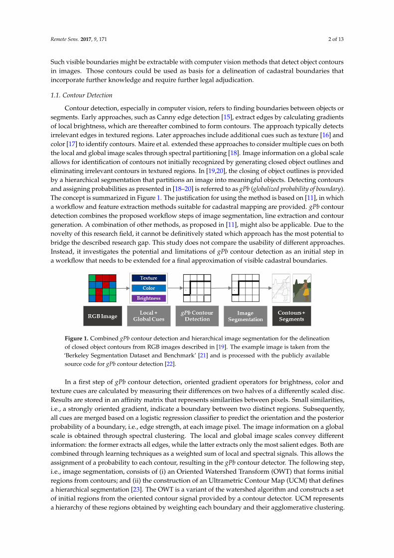
Figure 1. Combined gPb contour detection and hierarchical image segmentation for the delineation of closed object contours from RGB images described in [19]. The example image is taken from the ‘Berkeley Segmentation Dataset and Benchmark’ [21] and is processed with the publicly available source code for gPb contour detection [22].

In a first step of gPb contour detection, oriented gradient operators for brightness, color and texture cues are calculated by measuring their differences on two halves of a differently scaled disc. Results are stored in an affinity matrix that represents similarities between pixels. Small similarities, i.e., a strongly oriented gradient, indicate a boundary between two distinct regions. Subsequently, all cues are merged based on a logistic regression classifier to predict the orientation and the posterior probability of a boundary, i.e., edge strength, at each image pixel. The image information on a global scale is obtained through spectral clustering. The local and global image scales convey different information: the former extracts all edges, while the latter extracts only the most salient edges. Both are combined through learning techniques as a weighted sum of local and spectral signals. This allows the assignment of a probability to each contour, resulting in the gPb contour detector. The following step, i.e., image segmentation, consists of (i) an Oriented Watershed Transform (OWT) that forms initial regions from contours; and (ii) the construction of an Ultrametric Contour Map (UCM) that defines a hierarchical segmentation [23]. The OWT is a variant of the watershed algorithm and constructs a set of initial regions from the oriented contour signal provided by a contour detector. UCM represents a hierarchy of these regions obtained by weighting each boundary and their

Figure 1. Combined gPb contour detection and hierarchical image segmentation for the delineationof closed object contours from RGB images described in [19]. The example image is taken from the‘Berkeley Segmentation Dataset and Benchmark’ [21] and is processed with the publicly availablesource code for gPb contour detection [22].

In a first step of gPb contour detection, oriented gradient operators for brightness, color andtexture cues are calculated by measuring their differences on two halves of a differently scaled disc.Results are stored in an affinity matrix that represents similarities between pixels. Small similarities,i.e., a strongly oriented gradient, indicate a boundary between two distinct regions. Subsequently,all cues are merged based on a logistic regression classifier to predict the orientation and the posteriorprobability of a boundary, i.e., edge strength, at each image pixel. The image information on a globalscale is obtained through spectral clustering. The local and global image scales convey differentinformation: the former extracts all edges, while the latter extracts only the most salient edges. Both arecombined through learning techniques as a weighted sum of local and spectral signals. This allows theassignment of a probability to each contour, resulting in the gPb contour detector. The following step,i.e., image segmentation, consists of (i) an Oriented Watershed Transform (OWT) that forms initialregions from contours; and (ii) the construction of an Ultrametric Contour Map (UCM) that definesa hierarchical segmentation [23]. The OWT is a variant of the watershed algorithm and constructs a setof initial regions from the oriented contour signal provided by a contour detector. UCM representsa hierarchy of these regions obtained by weighting each boundary and their agglomerative clustering.

Remote Sens. 2017, 9, 171 3 of 13

The image segmentation, consisting of the two steps of OWT and UCM, can be applied to the output ofany contour detector. However, it has been proven to work optimally on the output of the gPb contourdetector [20]. The overall results are (i) a contour map, in which each pixel is assigned a probabilityfor being a boundary pixel; and (ii) a binary boundary map, in which each pixel is labeled as either‘boundary’ or ‘no boundary’ and from which closed segments can be derived. The number of contourstransferred from the contour map to closed segments in the boundary map is defined by a threshold,which is referred to as scale k in [19,20] and in the following. The processing pipeline of gPb-owt-ucmis referred to as gPb contour detection in this study.

gPb contour detection provides accurate results compared to other approaches on imagesegmentation (e.g., mean shift, multiscale normalized cuts and region merging) and edge detection (e.g.,Prewitt, Sobel, Roberts operator and Canny detector) [19] and is often referred to as a state-of-the-artmethod for contour detection [24–26]. These comparisons are based on computer vision images,while its performance on remote sensing data has not been evaluated as extensively against comparableapproaches. The main advantage of the method is its combination of edge detection and hierarchicalimage segmentation, while integrating image information on texture, color and brightness on a botha local and global scale. As the cue combination is learned, based on a large number of natural imagesfrom the ‘Berkeley Segmentation Dataset and Benchmark’ [21], the approach seeks to be transferable toimages of different contexts. Nevertheless, gPb contour detection has hardly been applied to remotelysensed data [27,28] and, to the best of the authors’ knowledge, never to UAV data. The transferability ofmethods from computer vision to remote sensing is challenging, as both are often developed for imagedata with different characteristics: a benchmark dataset used in computer vision, such as the ‘BerkeleySegmentation Dataset and Benchmark’, contains natural images of maximal 1000 pixels in width andheight, whereas a benchmark dataset used in remote sensing, such as the ‘ISPRS Benchmark’ [29],contains images from multiple sensors with higher numbers of pixels and larger ground sampledistances (GSD).

1.2. Objective and Organization of the Study

This study investigates which processing is required for a state-of-the-art contour detectionmethod from computer vision—namely gPb contour detection—to be applied to remotely senseddata with a high resolution—namely UAV data. Once the technical transferability is defined,the applicability of the method within the application field of cadastral mapping is investigated.This study aims to outline the potential of gPb contour detection for an automated delineation of visibleobjects that indicate cadastral boundaries.

Overall, the study addresses the research gaps of transferring a method developed withincomputer vision to an application in remote sensing, where images have different characteristics.Further, it encounters the lack of automation within cadastral boundary delineation by investigatingthe applicability of gPb contour detection.

The paper is structured as follows: after having described the context of this research (Section 1),the UAV datasets as well as the methodological approach are described (Section 2). Then, the resultsare described (Section 3) and discussed (Section 4). Concluding remarks include generic statementsabout the transferability and applicability of gPb contour detection for UAV-based delineation of visiblecadastral boundaries (Section 5).

2. Materials and Methods

2.1. UAV Data

Three UAV orthoimages of different extents showing rural areas in Germany, France and Indonesiawere selected for this study. Rural areas were chosen because the number of visible boundaries isusually higher in rural areas compared to high-density urban areas. For Amtsvenn and Lunyuk,data was captured with indirect georeferencing, i.e., Ground Control Points (GCPs) were distributed

Remote Sens. 2017, 9, 171 4 of 13

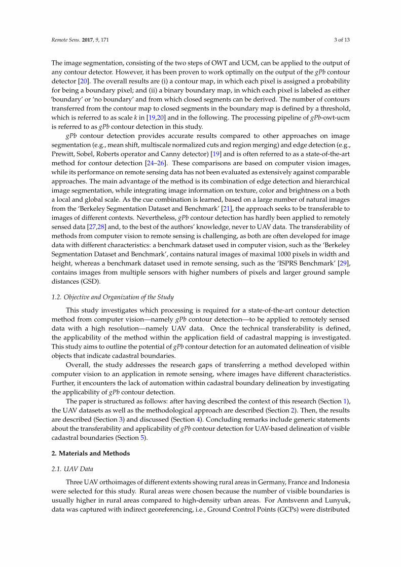
within the field and measured with a Global Navigation Satellite System (GNSS). For Toulouse,data was captured with direct georeferencing, i.e., through an on-board Post-Processing Kinematic(PPK) unit. All orthoimages were generated with Pix4DMapper. Table 1 shows specifications of thedata capture, while Figure 2 shows orthoimages of the study areas.

Table 1. Specifications of UAV datasets per study area.

Location Latitude/Longitude UAV Model Camera/FocalLength [mm]

OverlapForward/Sideward

[%]

GSD[cm] Extent [m] Pixels

Amtsvenn,Germany 52.17335/6.92865 GerMAP G180 Ricoh

GR/18.3 80/65 4.86 1000 × 1000 20,538 × 20,538

Toulouse,France 43.21596/0.99870 DT18 PPK DT-3Bands

RGB/5.5 80/70 3.61 500 × 500 13,816 × 13,816

Lunyuk,Indonesia −8.97061/117.21819 DJI Phantom 3 Sony EXMOR

FC300S/3.68 90/60 3.00 250 × 250 8344 × 8344

2.2. Reference Data

The study is based on the assumption that large portions of cadastral boundaries are visible [14].Therefore, the method is intended to extract contours of physical objects that demarcate cadastralboundaries. A general list of such objects is rarely available in the literature and strongly dependson the area of investigation [11]. From a list of objects provided in [11], the following objects wereassumed to indicate cadastral boundaries for the investigated study areas: roads, fences, hedges,stone walls, roof outlines, agricultural field outlines as well as outlines of tree groups. The contours ofthese objects were manually digitized for all three orthoimages (Figure 2). The reference data does notaim to delineate cadastral boundaries, since a subset of these, i.e., visible boundaries, are consideredin this study. Cadastral boundaries are assumed to be more regular than the outlines of visibleobjects delineated as reference data. A workflow for cadastral boundary delineation would need tocontain a step in which extracted contours are generalized to be more likely to be cadastral boundaries.This study is not designed to provide such a complete workflow; it seeks to delineate object contoursas a first workflow step. Further workflow steps as proposed in [11] would need to be added, in orderto derive data that is comparable with cadastral data.

Remote Sens. 2017, 9, 171 4 of 13

Kinematic (PPK) unit. All orthoimages were generated with Pix4DMapper. Table 1 shows specifications of the data capture, while Figure 2 shows orthoimages of the study areas.

Table 1. Specifications of UAV datasets per study area.

Location Latitude/Longitude UAV Model Camera/Focal Length [mm]

OverlapForward/Sideward

[%]

GSD [cm]

Extent [m]

Pixels

Amtsvenn, Germany

52.17335/6.92865 GerMAP G180 Ricoh

GR/18.3 80/65 4.86

1000 × 1000

20,538 × 20,538

Toulouse, France

43.21596/0.99870 DT18 PPK DT-3Bands RGB/5.5

80/70 3.61 500 × 500 13,816 × 13,816

Lunyuk, Indonesia

−8.97061/117.21819 DJI Phantom 3 Sony EXMOR FC300S/3.68

90/60 3.00 250 × 250 8344 × 8344

2.2. Reference Data

The study is based on the assumption that large portions of cadastral boundaries are visible [14]. Therefore, the method is intended to extract contours of physical objects that demarcate cadastral boundaries. A general list of such objects is rarely available in the literature and strongly depends on the area of investigation [11]. From a list of objects provided in [11], the following objects were assumed to indicate cadastral boundaries for the investigated study areas: roads, fences, hedges, stone walls, roof outlines, agricultural field outlines as well as outlines of tree groups. The contours of these objects were manually digitized for all three orthoimages (Figure 2). The reference data does not aim to delineate cadastral boundaries, since a subset of these, i.e., visible boundaries, are considered in this study. Cadastral boundaries are assumed to be more regular than the outlines of visible objects delineated as reference data. A workflow for cadastral boundary delineation would need to contain a step in which extracted contours are generalized to be more likely to be cadastral boundaries. This study is not designed to provide such a complete workflow; it seeks to delineate object contours as a first workflow step. Further workflow steps as proposed in [11] would need to be added, in order to derive data that is comparable with cadastral data.

(a) (b) (c)

Figure 2. Manually delineated object contours used as reference data to determine the detection quality overlaid on UAV orthoimages of (a) Amtsvenn, Germany; (b) Toulouse, France and (c) Lunyuk, Indonesia.

2.3. Image Processing Workflow

The method investigated, gPb contour detection, is open-source and available as a precompiled Matlab package [22]. This implementation was found to be inapplicable because of long computing time and insufficient memory when processing images of more than 1000 pixels in width and height. Therefore, an image processing workflow that reduces the original image size to 1000 × 1000 pixels was designed (Figure 3). The workflow consists of four steps, which are explained in the following. Apart from the Matlab implementation for gPb contour detection, all workflow steps were

Figure 2. Manually delineated object contours used as reference data to determine the detectionquality overlaid on UAV orthoimages of (a) Amtsvenn, Germany; (b) Toulouse, France and(c) Lunyuk, Indonesia.

2.3. Image Processing Workflow

The method investigated, gPb contour detection, is open-source and available as a precompiledMatlab package [22]. This implementation was found to be inapplicable because of long computingtime and insufficient memory when processing images of more than 1000 pixels in width andheight. Therefore, an image processing workflow that reduces the original image size to 1000 × 1000

Remote Sens. 2017, 9, 171 5 of 13

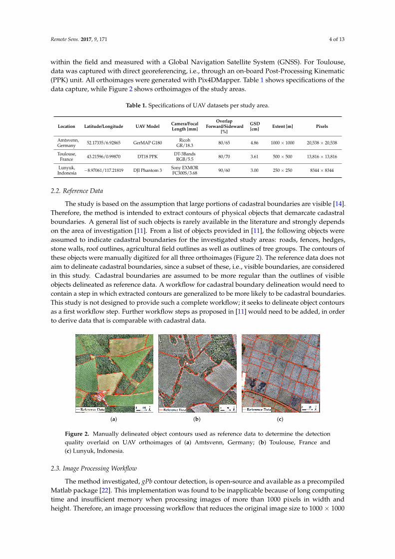
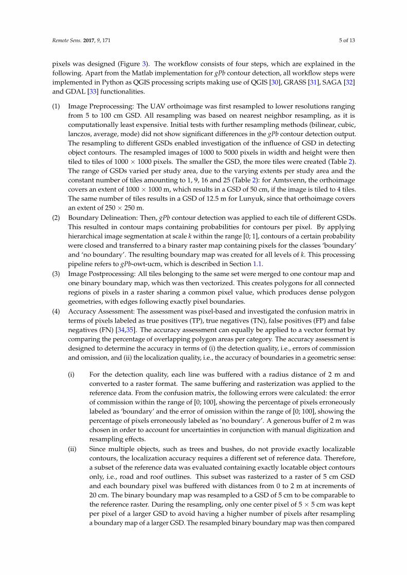
pixels was designed (Figure 3). The workflow consists of four steps, which are explained in thefollowing. Apart from the Matlab implementation for gPb contour detection, all workflow steps wereimplemented in Python as QGIS processing scripts making use of QGIS [30], GRASS [31], SAGA [32]and GDAL [33] functionalities.

(1) Image Preprocessing: The UAV orthoimage was first resampled to lower resolutions rangingfrom 5 to 100 cm GSD. All resampling was based on nearest neighbor resampling, as it iscomputationally least expensive. Initial tests with further resampling methods (bilinear, cubic,lanczos, average, mode) did not show significant differences in the gPb contour detection output.The resampling to different GSDs enabled investigation of the influence of GSD in detectingobject contours. The resampled images of 1000 to 5000 pixels in width and height were thentiled to tiles of 1000 × 1000 pixels. The smaller the GSD, the more tiles were created (Table 2).The range of GSDs varied per study area, due to the varying extents per study area and theconstant number of tiles amounting to 1, 9, 16 and 25 (Table 2): for Amtsvenn, the orthoimagecovers an extent of 1000 × 1000 m, which results in a GSD of 50 cm, if the image is tiled to 4 tiles.The same number of tiles results in a GSD of 12.5 m for Lunyuk, since that orthoimage coversan extent of 250 × 250 m.

(2) Boundary Delineation: Then, gPb contour detection was applied to each tile of different GSDs.This resulted in contour maps containing probabilities for contours per pixel. By applyinghierarchical image segmentation at scale k within the range [0; 1], contours of a certain probabilitywere closed and transferred to a binary raster map containing pixels for the classes ‘boundary’and ‘no boundary’. The resulting boundary map was created for all levels of k. This processingpipeline refers to gPb-owt-ucm, which is described in Section 1.1.

(3) Image Postprocessing: All tiles belonging to the same set were merged to one contour map andone binary boundary map, which was then vectorized. This creates polygons for all connectedregions of pixels in a raster sharing a common pixel value, which produces dense polygongeometries, with edges following exactly pixel boundaries.

(4) Accuracy Assessment: The assessment was pixel-based and investigated the confusion matrix interms of pixels labeled as true positives (TP), true negatives (TN), false positives (FP) and falsenegatives (FN) [34,35]. The accuracy assessment can equally be applied to a vector format bycomparing the percentage of overlapping polygon areas per category. The accuracy assessment isdesigned to determine the accuracy in terms of (i) the detection quality, i.e., errors of commissionand omission, and (ii) the localization quality, i.e., the accuracy of boundaries in a geometric sense:

(i) For the detection quality, each line was buffered with a radius distance of 2 m andconverted to a raster format. The same buffering and rasterization was applied to thereference data. From the confusion matrix, the following errors were calculated: the errorof commission within the range of [0; 100], showing the percentage of pixels erroneouslylabeled as ‘boundary’ and the error of omission within the range of [0; 100], showing thepercentage of pixels erroneously labeled as ‘no boundary’. A generous buffer of 2 m waschosen in order to account for uncertainties in conjunction with manual digitization andresampling effects.

(ii) Since multiple objects, such as trees and bushes, do not provide exactly localizablecontours, the localization accuracy requires a different set of reference data. Therefore,a subset of the reference data was evaluated containing exactly locatable object contoursonly, i.e., road and roof outlines. This subset was rasterized to a raster of 5 cm GSDand each boundary pixel was buffered with distances from 0 to 2 m at increments of20 cm. The binary boundary map was resampled to a GSD of 5 cm to be comparable tothe reference raster. During the resampling, only one center pixel of 5 × 5 cm was keptper pixel of a larger GSD to avoid having a higher number of pixels after resamplinga boundary map of a larger GSD. The resampled binary boundary map was then compared

Remote Sens. 2017, 9, 171 6 of 13

to the reference raster. Based on the confusion matrix, the number of TPs per buffer zonewas calculated to investigate the distance between TPs and the reference data and thusthe influence of GSD on the localization quality.

Remote Sens. 2017, 9, 171 6 of 13

Figure 3. Image processing workflow for delineation of visual object contours from UAV orthoimages and its assessment based on the comparison to reference data.

3. Results

Resampling and tiling the UAV orthoimages to tiles of 1000 × 1000 pixels results in a higher number of tiles for images of a smaller GSD (Table 2). Applying gPb contour detection on each tile of 1000 × 1000 pixels belonging to the same set of tiles with an identical GSD results in a contour map and a binary boundary map (Figure 4). The lower the level of k, the fewer contours are transferred from the contour map to the binary boundary map (Figure 5). The processing time for each tile ranged from 10 to 13 min and was 11 min on average, with gPb contour detection running single-threaded. The accuracy assessment is shown in terms of detection quality (Figure 6) and localization quality (Figure 7). To separate the influence of GSD and tiling on the detection quality, each untiled image of the largest GSD per study area was tiled to 25 tiles and assessed (Table 3).

Table 2. Number of pixels and ground sample distance (GSD) per tile after image preprocessing.

Pixels Tiles GSD (cm)Amtsvenn

GSD (cm)Toulouse

GSD (cm) Lunyuk

5000 × 5000 25 20 10 5 4000 × 4000 16 25 12.5 6.25 3000 × 3000 9 33 16.5 8.3 2000 × 2000 4 50 25 12.5 1000 × 1000 1 100 50 25

Table 3. Comparison of detection quality for images of largest ground sample distance (GSD) per study area for the untiled image and the same image merged from 25 tiles. Lower errors are marked in bold.

Amtsvenn Toulouse Lunyuk Pixels; GSD[cm] 1000 × 1000; 100 1000 × 1000; 50 1000 × 1000; 25

Tiles 1 25 1 25 1 25 Error of commission [%] 55.15 70.01 23.43 53.88 17.21 31.10

Error of omission [%] 13.44 68.75 27.44 90.12 52.30 96.24

Figure 3. Image processing workflow for delineation of visual object contours from UAV orthoimagesand its assessment based on the comparison to reference data.

3. Results

Resampling and tiling the UAV orthoimages to tiles of 1000 × 1000 pixels results in a highernumber of tiles for images of a smaller GSD (Table 2). Applying gPb contour detection on each tile of1000 × 1000 pixels belonging to the same set of tiles with an identical GSD results in a contour mapand a binary boundary map (Figure 4). The lower the level of k, the fewer contours are transferredfrom the contour map to the binary boundary map (Figure 5). The processing time for each tile rangedfrom 10 to 13 min and was 11 min on average, with gPb contour detection running single-threaded.The accuracy assessment is shown in terms of detection quality (Figure 6) and localization quality(Figure 7). To separate the influence of GSD and tiling on the detection quality, each untiled image ofthe largest GSD per study area was tiled to 25 tiles and assessed (Table 3).

Table 2. Number of pixels and ground sample distance (GSD) per tile after image preprocessing.

Pixels Tiles GSD (cm) Amtsvenn GSD (cm) Toulouse GSD (cm) Lunyuk

5000 × 5000 25 20 10 54000 × 4000 16 25 12.5 6.253000 × 3000 9 33 16.5 8.32000 × 2000 4 50 25 12.51000 × 1000 1 100 50 25

Table 3. Comparison of detection quality for images of largest ground sample distance (GSD) per studyarea for the untiled image and the same image merged from 25 tiles. Lower errors are marked in bold.

Amtsvenn Toulouse Lunyuk

Pixels; GSD[cm] 1000 × 1000; 100 1000 × 1000; 50 1000 × 1000; 25

Tiles 1 25 1 25 1 25

Error of commission [%] 55.15 70.01 23.43 53.88 17.21 31.10Error of omission [%] 13.44 68.75 27.44 90.12 52.30 96.24

Remote Sens. 2017, 9, 171 7 of 13Remote Sens. 2017, 9, 171 7 of 13

(a) (b) (c)

(d) (e) (f)

(g) (h) (i)

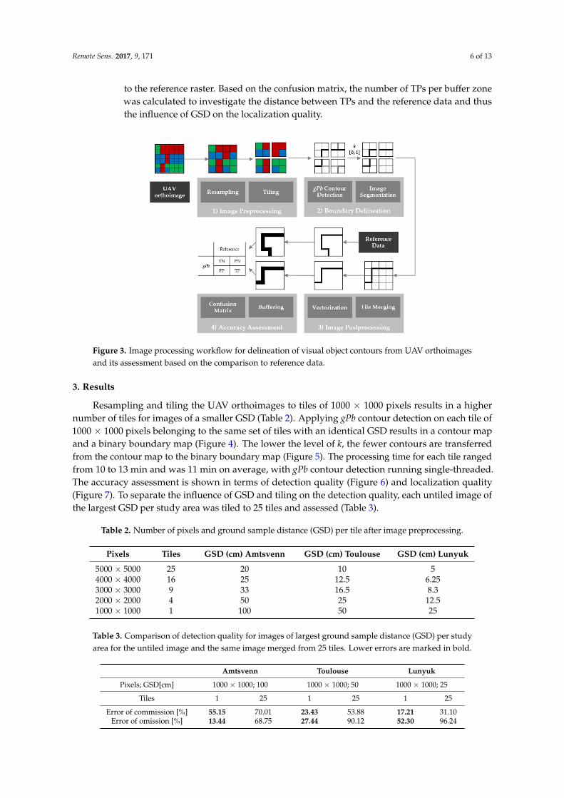
Figure 4. (a–i) Examples of contour maps (a,d,g) and binary boundary maps (k = 0.1) of Amtsvenn (a–c), Toulouse (d–f) and Lunyuk (g–i). The boundary maps are buffered with 2 m to increase their visibility. (a,b,d,e,g,h) result from an untiled input image of 1000 × 1000 pixels, (c,f,i) from an input image of 5000 × 5000 pixels merged from 25 tiles.

Figure 4. (a–i) Examples of contour maps (a,d,g) and binary boundary maps (k = 0.1) of Amtsvenn(a–c), Toulouse (d–f) and Lunyuk (g–i). The boundary maps are buffered with 2 m to increase theirvisibility. (a,b,d,e,g,h) result from an untiled input image of 1000 × 1000 pixels, (c,f,i) from an inputimage of 5000 × 5000 pixels merged from 25 tiles.Remote Sens. 2017, 9, 171 8 of 13

(a) (b) (c)

Figure 5. Binary boundary maps derived from untiled UAV orthoimage of Amtsvenn with a size of 1000 × 1000 pixels and 100 cm GSD at level (a) k = 0.1; (b) k = 0.3; and (c) k = 0.5.

(a) (b) (c)

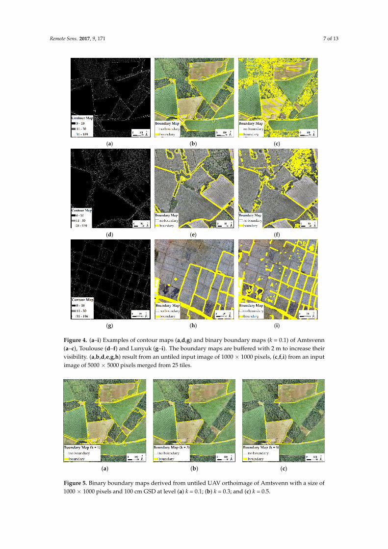
Figure 6. Detection quality: the errors of commission and omission is shown for binary boundary maps of different Ground Sample Distances (GSD) derived for (a) Amtsvenn; (b) Toulouse; and (c) Lunyuk at level k = 0.1.

(a) (b) (c)

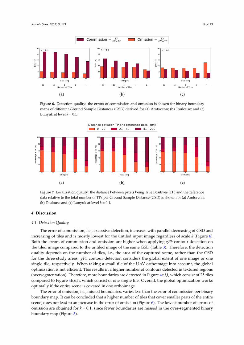
Figure 7. Localization quality: the distance between pixels being True Positives (TP) and the reference data relative to the total number of TPs per Ground Sample Distance (GSD) is shown for (a) Amtsvenn; (b) Toulouse and (c) Lunyuk at level k = 0.1.

4. Discussion

4.1. Detection Quality

The error of commission, i.e., excessive detection, increases with parallel decreasing of GSD and increasing of tiles and is mostly lowest for the untiled input image regardless of scale k (Figure 6). Both the errors of commission and omission are higher when applying gPb contour detection on the

Figure 5. Binary boundary maps derived from untiled UAV orthoimage of Amtsvenn with a size of1000 × 1000 pixels and 100 cm GSD at level (a) k = 0.1; (b) k = 0.3; and (c) k = 0.5.

Remote Sens. 2017, 9, 171 8 of 13

Remote Sens. 2017, 9, 171 8 of 13

(a) (b) (c)

Figure 5. Binary boundary maps derived from untiled UAV orthoimage of Amtsvenn with a size of 1000 × 1000 pixels and 100 cm GSD at level (a) k = 0.1; (b) k = 0.3; and (c) k = 0.5.

(a) (b) (c)

Figure 6. Detection quality: the errors of commission and omission is shown for binary boundary maps of different Ground Sample Distances (GSD) derived for (a) Amtsvenn; (b) Toulouse; and (c) Lunyuk at level k = 0.1.

(a) (b) (c)

Figure 7. Localization quality: the distance between pixels being True Positives (TP) and the reference data relative to the total number of TPs per Ground Sample Distance (GSD) is shown for (a) Amtsvenn; (b) Toulouse and (c) Lunyuk at level k = 0.1.

4. Discussion

4.1. Detection Quality

The error of commission, i.e., excessive detection, increases with parallel decreasing of GSD and increasing of tiles and is mostly lowest for the untiled input image regardless of scale k (Figure 6). Both the errors of commission and omission are higher when applying gPb contour detection on the

Figure 6. Detection quality: the errors of commission and omission is shown for binary boundarymaps of different Ground Sample Distances (GSD) derived for (a) Amtsvenn; (b) Toulouse; and (c)Lunyuk at level k = 0.1.

Remote Sens. 2017, 9, 171 8 of 13

(a) (b) (c)

Figure 5. Binary boundary maps derived from untiled UAV orthoimage of Amtsvenn with a size of 1000 × 1000 pixels and 100 cm GSD at level (a) k = 0.1; (b) k = 0.3; and (c) k = 0.5.

(a) (b) (c)

Figure 6. Detection quality: the errors of commission and omission is shown for binary boundary maps of different Ground Sample Distances (GSD) derived for (a) Amtsvenn; (b) Toulouse; and (c) Lunyuk at level k = 0.1.

(a) (b) (c)

Figure 7. Localization quality: the distance between pixels being True Positives (TP) and the reference data relative to the total number of TPs per Ground Sample Distance (GSD) is shown for (a) Amtsvenn; (b) Toulouse and (c) Lunyuk at level k = 0.1.

4. Discussion

4.1. Detection Quality

The error of commission, i.e., excessive detection, increases with parallel decreasing of GSD and increasing of tiles and is mostly lowest for the untiled input image regardless of scale k (Figure 6). Both the errors of commission and omission are higher when applying gPb contour detection on the

Figure 7. Localization quality: the distance between pixels being True Positives (TP) and the referencedata relative to the total number of TPs per Ground Sample Distance (GSD) is shown for (a) Amtsvenn;(b) Toulouse and (c) Lunyuk at level k = 0.1.

4. Discussion

4.1. Detection Quality

The error of commission, i.e., excessive detection, increases with parallel decreasing of GSD andincreasing of tiles and is mostly lowest for the untiled input image regardless of scale k (Figure 6).Both the errors of commission and omission are higher when applying gPb contour detection onthe tiled image compared to the untiled image of the same GSD (Table 3). Therefore, the detectionquality depends on the number of tiles, i.e., the area of the captured scene, rather than the GSDfor the three study areas: gPb contour detection considers the global extent of one image or onesingle tile, respectively. When taking a small tile of the UAV orthoimage into account, the globaloptimization is not efficient. This results in a higher number of contours detected in textured regions(oversegmentation). Therefore, more boundaries are detected in Figure 4c,f,i, which consist of 25 tilescompared to Figure 4b,e,h, which consist of one single tile. Overall, the global optimization worksoptimally if the entire scene is covered in one orthoimage.

The error of omission, i.e., missed boundaries, varies less than the error of commission per binaryboundary map. It can be concluded that a higher number of tiles that cover smaller parts of the entirescene, does not lead to an increase in the error of omission (Figure 6). The lowest number of errors ofomission are obtained for k = 0.1, since fewer boundaries are missed in the over-segmented binaryboundary map (Figure 5).

Remote Sens. 2017, 9, 171 9 of 13

The overall detection accuracy is close to 100%, since many pixels are classified correctly as ‘noboundary’. It is therefore not visualized in Figure 6. A low level of k leads to an oversegmentationof the image, while a higher level of k leads to an undersegmentation or even no boundaries beingcontained in the binary boundary map (Figure 5), which influences the errors of commission andomission accordingly. However, even for the lowest level of k, contours indicated in the contour map(Figure 4g) might not be transferred to the binary boundary map (Figure 4h). This indicates thatwhen aiming for a high completeness of detected contours, i.e., a low error of omission, which isconsidered optimal in [36] before integrating user interaction, the contour map should be consideredfor further processing.

The results for Amtsvenn show the highest number of errors of commission, due to many texturedregions in which boundaries are erroneously detected. The error of commission is lowest for Lunyuk,since the image contains barely any textured regions or small objects. The high errors of omission forthe Toulouse and Lunyuk data reveal that boundaries are less definite and visible in these images.

4.2. Localization Quality

The number of TPs within 20 cm distance of the reference data relative to the total numberof TPs per GSD decreases for larger GSDs, for all study areas (Figure 7). The total number of TPswas comparable, as only one center pixel was kept in the gPb contour detection raster of 5 cm GSDthat was compared to the reference data of the same GSD. For GSDs of 20–33 cm (Amtsvenn) and10–25 cm (Toulouse and Lunyuk), the amount of TP localized within 20 cm distance from the referencedata ranges between 50% and 60%. This percentage decreases for all study areas when the GSD isincreased to 100 cm. The results indicate that contours are more accurately localized for UAV imagesof a higher resolution.

4.3. Discussion of the Evaluation Approach

The study results (Section 4.1, Section 4.2) strongly depend on the applied buffer distance.For detection quality, a buffer distance of 2 m was chosen. This does not represent the followingtwo visually observed cases: (i) some boundaries run along the shadow of an object and aretherefore shifted compared to the reference data that runs along the actual object contour; (ii) someboundaries are covered by other objects, e.g., trees covering streets. Merging contours of smallerobjects with the applied buffer distance does not represent such cases. Such issues could be resolvedwith an object detection that includes semantics, i.e., knowledge about the objects to be extracted.UAV-based approaches have the potential to extract such object knowledge through incorporationof high-resolution imagery, pointclouds and DSMs. According to Mayer, the use of such additionalinformation makes object extraction more robust and reliable [36]. The approach to detection quality isemployed similarly in other studies [34,35,37,38]. The authors argue that despite its strong dependencyon the buffer size and its focus on positional accuracy while neglecting factors such as topologicalaccuracy, the buffer approach provides a simple and comprehensive accuracy measure. Further, it canbe used on both a vector and a raster representation and is easy to implement [38]. For a comparisonto cadastral data, a smaller buffer size, according to local accuracy requirements, should be considered.

Apart from the accuracy assessment method, the manually drawn reference data stronglyinfluences the results. Manually drawn reference data is argued to be valid for measuring the degree towhich an automated system, as proposed in this study, outperforms a human operator [36]. However,each human might draw different reference data. Averaging a large amount of manually drawnreference data, as proposed in [17], might reduce errors produced by an individual. Manually drawnreference data was chosen instead of real cadastral data, as the approach does not aim to delineate finalcadastral boundaries, but the outlines of physical objects demarcating visible cadastral boundaries.To which extent these visible boundaries coincide with cadastral data, appears to be highlycase-depended and needs to be investigated in future work. Our approach is designed for casesin which cadastral data is largely visible.

Remote Sens. 2017, 9, 171 10 of 13

4.4. Transferability and Applicability of gPb for Boundary Delineation

gPb contour detection appears to be transferable to UAV orthoimages, when reducing the images’resolution. The approach shows potential for the automation of cadastral boundary delineation incases where cadastral maps are scarcely available and concepts such as fit-for-purpose and responsibleland administration are in place [39,40]. Such concepts accept general boundaries, for which thepositional correctness is of lower importance [14]. In cases where a map needs to be created or updated,and general boundaries are accepted, editing automatically generated visible boundaries of highcompleteness, correctness and topological accuracy on a UAV orthoimage might be less cost- andtime-intensive than manually digitizing all boundaries. This would need to be verified by comparingboth cadastral mapping workflows as a whole. Hence, future work is required to determine to whichdegree the object contours coincide with cadastral boundaries and which level of accuracy is required tooutperform a manual cadastral mapping workflow. For road extraction, which is closely related to theobject detection of this study, Mayer et al. propose a correctness of around 85% and a completeness ofaround 70% for an approach to be of real practical importance, which relates to an error of commissionof 15% and an error of omission of 30% [41]. Such values can hardly be achieved when applyingsolely gPb contour detection for cadastral boundary delineation. The contours of gPb contour detectionshould be considered as an initial workflow step in a complete processing chain, as proposed in [11].One idea would be to use the gPb contour detection for a general localization of potential visibleboundaries and to integrate further approaches taking into account the full resolution provided byUAVs to decide on the final probability and localization for a visible boundary. Those boundarieswould then need to be connected and regularized to form a closed network of potential cadastralboundaries, before integrating human interaction. Once such a complete workflow is developed,a comparison to direct techniques and indirect techniques using aerial or satellite images of lowerresolutions is feasible. However, even if UAV-based cadastral mapping fulfills the expected criteria,the approach is unlikely to substitute convention approaches, as UAVs are currently not suitable tomap large areas and are limited in use due to regulations [5].

Furthermore, there might be cases in which only a small portion of cadastral boundaries isvisible or object contours do not coincide with cadastral boundaries. Then, the proposed data-drivenapproach will need to be combined with a knowledge-driven approach. To reliably delineate a closedand geometrically and topologically correct network of boundaries, further object knowledge shouldbe incorporated, e.g., through semi-supervised machine learning approaches and thus derivedcomplementary data. The contour map containing the probability for each contour detected and forwhich the level of k does not need to be defined, could be employed as a first workflow step. The salientcontours detected in this step could be balanced by incorporating an area-based segmentation,resulting in more homogeneous areas. Adding further steps to the workflow could generate an outputdirectly comparable to cadastral boundaries. In future, the authors aim to develop a workflow thatremains as automatic, generic and adaptive to different scenarios as possible, similarly formulatedin [42] as a need for contemporary boundary detection schemes.

5. Conclusions

This study examines the recent endeavor of making the process of cadastral mapping morereproducible, transparent, automated, scalable and cost-effective. This is investigated by proposingthe application of UAV orthoimages combined with automated image analysis, i.e., a state-of-the-artcomputer vision method that has never been applied to UAV data. The approach does not requireprior knowledge (learning) and automatically detects object contours from UAV orthoimages thatindicate visible cadastral boundaries. More specifically, this study investigates the transferabilityof gPb contour detection to UAV images and its applicability for automated delineation of objectsdemarcating visible cadastral boundaries. This is investigated in terms of detection and localizationquality for three different study areas.

Remote Sens. 2017, 9, 171 11 of 13

The results show the potential and limitations of gPb contour detection within the describedapplication field. The approach is most suitable for areas in which object contours are clearly visibleand coincide with cadastral boundaries. However, the approach is of limited usability as a standaloneapproach for cadastral mapping: it can be employed for an initial localization of candidate objectboundaries, which need to be verified and located exactly by integrating further workflow steps.The design and implementation of such a complete workflow that incorporates the high resolutionthat UAV data provides is the focus of our future work. To establish the comparability of the detectedobject contours with cadastral boundaries, future work will focus on incorporating the approachproposed here with machine learning methods to integrate further object knowledge. The goal is togenerate a tool for cadastral boundary delineation that is highly automatic, generic and adaptive todifferent scenarios.

Acknowledgments: This work was supported by its4land, which is part of the Horizon 2020 program of theEuropean Union (project number 687828). We are grateful to Claudia Stöcker, Sheilla Ayu Ramadhani andDelAirTech for capturing, processing and providing the UAV data. We acknowledge the financial support of theOpen Science Fund of the University of Twente, which supports open access publishing.

Author Contributions: Sophie Crommelinck processed all the data for this paper. Markus Gerke, Rohan Bennett,Michael Ying Yang and George Vosselman contributed to the analysis and interpretation of the data.The manuscript was written by Sophie Crommelinck with contributions from Markus Gerke, Rohan Bennett,Michael Ying Yang and George Vosselman.

Conflicts of Interest: The authors declare no conflict of interest.

Abbreviations

The following abbreviations are used in this manuscript:

DSM Digital Surface ModelFN False NegativeFP False PositiveGCP Ground Control PointsGNSS Global Navigation Satellite SystemgPb Globalized Probability of BoundaryGSD Ground Sample DistanceOWT Oriented Watershed TransformPPK Post Processing KinematicTN True NegativeTP True PositiveUAV Unmanned Aerial VehicleUCM Ultrametric Contour Map

References

1. Colomina, I.; Molina, P. Unmanned aerial systems for photogrammetry and remote sensing: A review.ISPRS J. Photogramm. Remote Sens. 2014, 92, 79–97. [CrossRef]

2. Nex, F.; Remondino, F. UAV for 3D mapping applications: A review. Appl. Geomat. 2014, 6, 1–15. [CrossRef]3. Pajares, G. Overview and current status of remote sensing applications based on unmanned aerial vehicles

(UAVs). Photogramm. Eng. Remote Sens. 2015, 81, 281–329. [CrossRef]4. Manyoky, M.; Theiler, P.; Steudler, D.; Eisenbeiss, H. Unmanned aerial vehicle in cadastral applications.

Int. Arch. Photogramm. Remote Sens. Spat. Inf. Sci. 2011, 63, 1–6. [CrossRef]5. Barnes, G.; Volkmann, W. High-resolution mapping with unmanned aerial systems. Surv. Land Inf. Sci. 2015,

74, 5–13.6. Mumbone, M.; Bennett, R.; Gerke, M.; Volkmann, W. Innovations in boundary mapping: Namibia, customary

lands and UAVs. In Proceedings of the World Bank Conference on Land and Poverty, Washington, DC, USA,23–27 March 2015; pp. 1–22.

7. Volkmann, W.; Barnes, G. Virtual surveying: Mapping and modeling cadastral boundaries using UnmannedAerial Systems (UAS). In Proceedings of the FIG Congress: Engaging the Challenges—Enhancing theRelevance, Kuala Lumpur, Malaysia, 16–21 June 2014; pp. 1–13.

Remote Sens. 2017, 9, 171 12 of 13

8. Maurice, M.J.; Koeva, M.N.; Gerke, M.; Nex, F.; Gevaert, C. A photogrammetric approach for map updatingusing UAV in Rwanda. In Proceedings of the GeoTech Rwanda—International Conference on GeospatialTechnologies for Sustainable Urban and Rural Development, Kigali, Rwanda, 18–20 November 2015; pp. 1–8.

9. Binns, B.O.; Dale, P.F. Cadastral Surveys and Records of Rights in Land Administration. Available online:http://www.fao.org/docrep/006/v4860e/v4860e03.htm (accessed on 10 November 2016).

10. Williamson, I.; Enemark, S.; Wallace, J.; Rajabifard, A. Land Administration for Sustainable Development;ESRI Press Academic: Redlands, CA, USA, 2010; p. 472.

11. Crommelinck, S.; Bennett, R.; Gerke, M.; Nex, F.; Yang, M.; Vosselman, G. Review of automatic featureextraction from high-resolution optical sensor data for UAV-based cadastral mapping. Remote Sens. 2016, 8,1–28. [CrossRef]

12. Jazayeri, I.; Rajabifard, A.; Kalantari, M. A geometric and semantic evaluation of 3D data sourcing methodsfor land and property information. Land Use Policy 2014, 36, 219–230. [CrossRef]

13. Bennett, R.; Kitchingman, A.; Leach, J. On the nature and utility of natural boundaries for land and marineadministration. Land Use policy 2010, 27, 772–779. [CrossRef]

14. Zevenbergen, J.; Bennett, R. The visible boundary: More than just a line between coordinates. In Proceedingsof the GeoTech Rwanda—International Conference on Geospatial Technologies for Sustainable Urban andRural Development, Kigali, Rwanda, 18–20 November 2015; pp. 1–4.

15. Canny, J. A computational approach to edge detection. IEEE Trans. Pattern Anal. Mach. Intell. 1986, 6,679–698. [CrossRef]

16. Malik, J.; Belongie, S.; Leung, T.; Shi, J. Contour and texture analysis for image segmentation. Int. J.Comput. Vis. 2001, 43, 7–27. [CrossRef]

17. Martin, D.R.; Fowlkes, C.C.; Malik, J. Learning to detect natural image boundaries using local brightness,color, and texture cues. IEEE Trans. Pattern Anal. Mach. Intell. 2004, 26, 530–549. [CrossRef] [PubMed]

18. Maire, M.; Arbeláez, P.; Fowlkes, C.; Malik, J. Using contours to detect and localize junctions in naturalimages. In Proceedings of the IEEE Conference on Computer Vision and Pattern Recognition, Anchorage,AK, USA, 23–28 June 2008; pp. 1–8.

19. Arbelaez, P.; Maire, M.; Fowlkes, C.; Malik, J. Contour detection and hierarchical image segmentation.Pattern Anal. Mach. Intell. 2011, 33, 898–916. [CrossRef] [PubMed]

20. Arbelaez, P.; Maire, M.; Fowlkes, C.; Malik, J. From contours to regions: An empirical evaluation.In Proceedings of the IEEE Conference on Computer Vision and Pattern Recognition (CVPR), Miami Beach,FL, USA, 20–25 June 2009; pp. 2294–2301.

21. Arbeláez, P.; Fowlkes, C.; Martin, D. Berkeley Segmentation Dataset and Benchmark. Available online:https://www2.eecs.berkeley.edu/Research/Projects/CS/vision/bsds/ (accessed on 10 November 2016).

22. Arbeláez, P.; Maire, M.; Fowlkes, C.; Malik, J. Contour Detection and Image Segmentation Resources.Available online: https://www2.eecs.berkeley.edu/Research/Projects/CS/vision/grouping/resources.html(accessed on 10 November 2016).

23. Arbelaez, P. Boundary extraction in natural images using ultrametric contour maps. In Proceedings ofthe Conference on Computer Vision and Pattern Recognition Workshop (CVPRW), New York, NY, USA,17–22 June 2006. [CrossRef]

24. Jevnisek, R.J.; Avidan, S. Semi global boundary detection. Comput. Vis. Image Understand. 2016, 152, 21–28.[CrossRef]

25. Zhang, X.; Xiao, P.; Song, X.; She, J. Boundary-constrained multi-scale segmentation method for remotesensing images. ISPRS J. Photogramm. Remote Sens. 2013, 78, 15–25. [CrossRef]

26. Szeliski, R. Computer Vision: Algorithms and Applications; Springer: London, UK, 2010; p. 812.27. Dornaika, F.; Moujahid, A.; El Merabet, Y.; Ruichek, Y. Building detection from orthophotos using a machine

learning approach: An empirical study on image segmentation and descriptors. Expert Syst. Appl. 2016, 58,130–142. [CrossRef]

28. Hou, B.; Kou, H.; Jiao, L. Classification of polarimetric SAR images using multilayer autoencoders andsuperpixels. IEEE J. Sel. Top. Appl. Earth Observ. Remote Sens. 2016, 9, 3072–3081. [CrossRef]

29. Rottensteiner, F.; Sohn, G.; Gerke, M.; Wegner, J.D.; Breitkopf, U.; Jung, J. Results of the ISPRS benchmark onurban object detection and 3D building reconstruction. ISPRS J. Photogramm. Remote Sens. 2014, 93, 256–271.[CrossRef]

Remote Sens. 2017, 9, 171 13 of 13

30. QGIS Development Team. QGIS Geographic Information System; Open Source Geospatial Foundation: Chicago,CA, USA, 2009. Available online: www.qgis.osgeo.org (accessed on 21 June 2016).

31. GRASS Developmnet Team. Geographic Resources Analysis Support System (GRASS) Software, Version 7.0.Available online: www.grass.osgeo.org (accessed on 21 June 2016).

32. Conrad, O.; Bechtel, B.; Bock, M.; Dietrich, H.; Fischer, E.; Gerlitz, L.; Wehberg, J.; Wichmann, V.; Böhner, J.System for automated geoscientific analyses (SAGA) Version 2.1.4. Geosci. Model Dev. 2015, 8, 1991–2007.[CrossRef]

33. GDAL Development Team. GDAL—Geospatial Data Abstraction Library, version 2.1.2; Open Source GeospatialFoundation: Chicago, CA, USA, 2016. Available online: www.gdal.org (accessed on 5 January 2017).

34. Wiedemann, C.; Heipke, C.; Mayer, H.; Jamet, O. Empirical evaluation of automatically extracted road axes.In Empirical Evaluation Techniques in Computer Vision; IEEE Computer Society Press: Los Alamitos, CA, USA,1998; pp. 172–187.

35. Shi, W.; Cheung, C.K.; Zhu, C. Modelling error propagation in vector-based buffer analysis. Int. J. Geogr.Inf. Sci. 2003, 17, 251–271. [CrossRef]

36. Mayer, H. Object extraction in photogrammetric computer vision. ISPRS J. Photogramm. Remote Sens. 2008,63, 213–222.

37. Kumar, M.; Singh, R.; Raju, P.; Krishnamurthy, Y. Road network extraction from high resolution multispectralsatellite imagery based on object oriented techniques. ISPRS Ann. Photogramm. Remote Sens. Spat. Inf. Sci.2014, 2, 107–110. [CrossRef]

38. Goodchild, M.F.; Hunter, G.J. A simple positional accuracy measure for linear features. Int. J. Geogr. Inf. Sci.1997, 11, 299–306. [CrossRef]

39. Enemark, S.; Bell, K.C.; Lemmen, C.; McLaren, R. Fit-For-Purpose Land Administration; International Federationof Surveyors: Frederiksberg, Denmark, 2014; p. 42.

40. Zevenbergen, J.; de Vries, W.; Bennett, R.M. Advances in Responsible Land Administration; CRC Press: Padstow,UK, 2015; p. 279.

41. Mayer, H.; Hinz, S.; Bacher, U.; Baltsavias, E. A test of automatic road extraction approaches. ISPRS Int. Arch.Photogramm. Remote Sens. Spat. Inform. Sci. 2006, 36, 209–214.

42. Basaeed, E.; Bhaskar, H.; Al-Mualla, M. CNN-based multi-band fused boundary detection for remotelysensed images. In Proceedings of the International Conference on Imaging for Crime Prevention andDetection, London, UK, 15–17 July 2015; pp. 1–6.

© 2017 by the authors; licensee MDPI, Basel, Switzerland. This article is an open accessarticle distributed under the terms and conditions of the Creative Commons Attribution(CC BY) license (http://creativecommons.org/licenses/by/4.0/).