contouring and isosurfaces - cgl @ ethz › ... › notes › slides › 02-contouring.pdf · basic...
TRANSCRIPT

Contouring and Isosurfaces
Ronald Peikert SciVis 2007 - Contouring 2-1
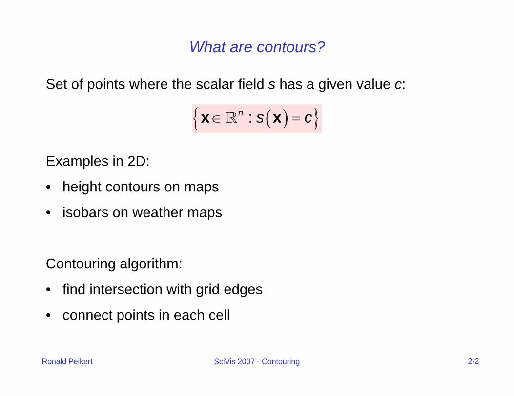
What are contours?
Set of points where the scalar field s has a given value c:
( ){ }:n s c∈ =x x
Examples in 2D:
( ){ }
• height contours on maps
• isobars on weather maps
Contouring algorithm:
• find intersection with grid edges
• connect points in each cell
Ronald Peikert SciVis 2007 - Contouring 2-2

Example
2 types of degeneracies:yp g• isolated points (c=6)• flat regions (c=8)
Ronald Peikert SciVis 2007 - Contouring 2-3
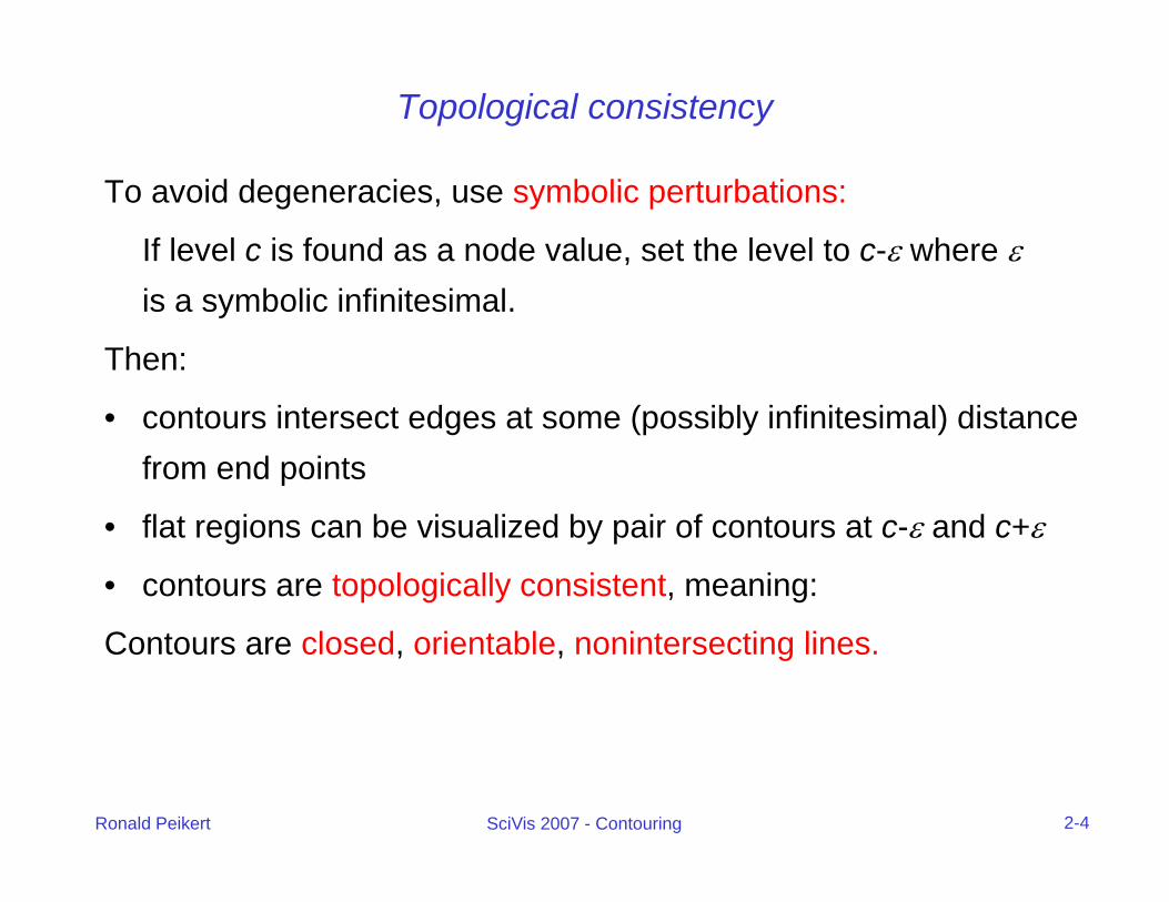
Topological consistency
To avoid degeneracies, use symbolic perturbations:
If level c is found as a node value, set the level to c-ε where εis a symbolic infinitesimal.
Then:
• contours intersect edges at some (possibly infinitesimal) distance from end points
• flat regions can be visualized by pair of contours at c-ε and c+ε
• contours are topologically consistent, meaning:
Contours are closed, orientable, nonintersecting lines.
Ronald Peikert SciVis 2007 - Contouring 2-4

Ambiguities of contours
What is the correct contour of c=4?
Two possibilities, both are orientable:
• values s(x)>c are on the left side
• values s(x)<c are on the right side
Answer: correctness depends on interior values of s(x).
But different interpolation schemes are possible.
Better question: What is the correct contour with respect to bilinear interpolation?
Ronald Peikert SciVis 2007 - Contouring 2-5

( ) ( ) ( ) ( )
Contours in a quadrangle cell
• local coordinates:• function values:• bilinear interpolant:
( ) ( ) ( ) ( )0,0 , 1,0 , 0,1 , 1,100 10 01 11, , ,s s s s
bilinear interpolant:
( )( ) ( ) ( )00 10 01 111 1 1 1s x y s x y s x y s x y s= − − + − + − +
Axy Bx Cy D+ + +
If A=0, contour equation is
Axy Bx Cy D= + + +
c Bx Cy D= + +contours are straight lines, all parallel
If A≠0 contour equation isC B BCc A x y D⎛ ⎞⎛ ⎞= + + + −⎜ ⎟⎜ ⎟If A≠0, contour equation is
contours are hyperbola, except for level
c A x y DA A A
+ + +⎜ ⎟⎜ ⎟⎝ ⎠⎝ ⎠
BCc DA
= −
Ronald Peikert SciVis 2007 - Contouring 2-6
A

Contours in a quadrangle cell
C B⎛ ⎞⎛ ⎞Contour equation for special level:
Contour is a pair of axis-aligned straight lines /x C A= −
0 C BA x yA A
⎛ ⎞⎛ ⎞= + +⎜ ⎟⎜ ⎟⎝ ⎠⎝ ⎠
Contour is a pair of axis aligned straight lines and .
/x C A=/y B A= −
Applied to example:• contour equation:
( )( )10 0 3 0 5 4 5
• special level c=4.5
( )( )10 0.3 0.5 4.5c x y= − − − +
• saddle point at (0.3, 0.5)
Ronald Peikert SciVis 2007 - Contouring 2-7

Contours in a quadrangle cell
Decision can be made without computing special level or saddle point, by comparing fractions of edges:
Using local coordinates, this works also for curvilinear and unstructured grids.
Ronald Peikert SciVis 2007 - Contouring 2-8

Contours in a quadrangle cell
Note: For drawing, straight lines are sufficient.Drawing hyperbola does not lead to better contours:
n
Reason: piecewise bilinear function is not C1.
Ronald Peikert SciVis 2007 - Contouring 2-9

Contours in a quadrangle cell
Basic contouring algorithms:• cell-by-cell algorithms: simple structure, but generate
disconnected segments, require post-processingg , q p p g• contour propagation methods: more complicated, but
generate connected contours
"Marching squares" algorithm (systematic cell-by-cell):• process nodes in ccw order denoted here as 0 1 2 3, , ,x x x xprocess nodes in ccw order, denoted here as• compute at each node the reduced field
(which is forced to be nonzero)th
0 1 2 3, , ,x x x x
( ) ( ) ( )i is s c ε= − −x xix
• take its sign as the ith bit of a 4-bit integer• use this as an index for lookup table containing the connectivity
information:
Ronald Peikert SciVis 2007 - Contouring 2-10

Contours in a quadrangle cell
( ) 0
0 1 2 3( ) 0is >x
( ) 0is <x
Alternating signs exist i 6 d 9
0 1 2 3
in cases 6 and 9.Choose the solid or
dashed line?
4 5 6 7
Both are possible for topological consistency
8 9 10 11consistency.
This allows to have a fixed table of 16 cases12 13 14 15
Ronald Peikert SciVis 2007 - Contouring 2-11
cases.

Contours in triangle/tetrahedral cells
Linear interpolation of cells impliespiece-wise linear contours.
Contours are unambiguous, making"marching triangles" even simpler than"marching squares"marching squares .
Question: Why not split quadrangles into two triangles (and hexahedra into five or six tetrahedra) and use marching triangles (tetrahedra)?
Answer: This can introduce periodic artifacts!
Ronald Peikert SciVis 2007 - Contouring 2-12

Contours in triangle/tetrahedral cells
Illustrative example: Find contour at level c=40.0 !
60.0 50.0 45.0 42.5
20.0 30.0 35.0 37.5
original quad grid, yielding vertices and contourtriangulated grid, yielding vertices and contour
Ronald Peikert SciVis 2007 - Contouring 2-13

Contours in triangle/tetrahedral cells
3D example based on real (downsampled) dataset.Contour (=isosurface) in
original hexahedral grid vs. in tetrahedrized grid:
Ronald Peikert SciVis 2007 - Contouring 2-14

The marching cubes algorithm
Contours of 3D scalar fields are known as isosurfaces.Before 1987, isosurfaces were computed as • contours on planar slices followed bycontours on planar slices, followed by• "contour stitching".
The marching cubes algorithm computes contours directly in 3D.• Pieces of the isosurfaces are generated on a cell-by-cell basis. • Similar to marching squares a 8 bit number is computed from• Similar to marching squares, a 8-bit number is computed from
the 8 signs of on the corners of a hexahedral cell.• The isosurface piece is looked up in a table with 256 entries.
( )is x
Ronald Peikert SciVis 2007 - Contouring 2-15

The marching cubes algorithm
How to build up the table of 256 cases?
Lorensen and Cline (1987) exploited 3 types of symmetries:Lorensen and Cline (1987) exploited 3 types of symmetries:• rotational symmetries of the cube• reflective symmetries of the cube• sign changes of
They published a reduced set of 14*) cases shown on the next
( )s x
They published a reduced set of 14 ) cases shown on the next slides where
• white circles indicate positive signs of ( )s x• the positive side of the isosurface is drawn in red, the negative
side in blue.
Ronald Peikert SciVis 2007 - Contouring 2-16
*) plus an unnecessary "case 14" which is a symmetric image of case 11.

The marching cubes algorithm
case 0 case 1 case 2 case 3
case 4 case 5 case 6 case 7
Ronald Peikert SciVis 2007 - Contouring 2-17
case 4 case 5 case 6 case 7

The marching cubes algorithm
case 8 case 9 case 10 case 11
case 12 case 13
Ronald Peikert SciVis 2007 - Contouring 2-18
case 12 case 13

The marching cubes algorithm
Do the pieces fit together?• The correct isosurfaces of the trilinear
interpolant would fit (trilinear reduces to p (bilinear on the cell interfaces)
• but the marching cubes polygons don't necessarily fitnecessarily fit.
Examplecase 10
• case 10, on top of• case 3 (rotated, signs changed)have matching signs at nodes but polygonshave matching signs at nodes but polygons
don't fit.
case 3
Ronald Peikert SciVis 2007 - Contouring 2-19
case 3
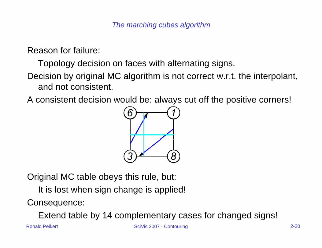
The marching cubes algorithm
Reason for failure: Topology decision on faces with alternating signs.
Decision by original MC algorithm is not correct w r t the interpolantDecision by original MC algorithm is not correct w.r.t. the interpolant, and not consistent.
A consistent decision would be: always cut off the positive corners!
Original MC table obeys this rule, but: It is lost when sign change is applied!
Consequence:
Ronald Peikert SciVis 2007 - Contouring 2-20
Consequence: Extend table by 14 complementary cases for changed signs!

The marching cubes algorithm
case 7case 3 case 6
case 3c case 6c case 7c
Ronald Peikert SciVis 2007 - Contouring 2-21
case 3c case 6c case 7c

The marching cubes algorithm
The remaining complementary cases are obtained simply by changing the orientation.
Example:p
case 1 case 1c
Based on the 28 cases, the full 256 cases are obtained by
case 1 case 1c
• rotations of the cube• reflections of the cube (and re-orienting of triangles)
Ronald Peikert SciVis 2007 - Contouring 2-22

The marching cubes algorithm
Summary of marching cubes algorithm:
Pre-processing steps:Pre processing steps:• build a table of the 28 cases• derive a table of the 256 cases, containing info on
– intersected cell edges, e.g. for case 3/256 (see case 2/28):(0,2), (0,4), (1,3), (1,5)
– triangles based on these points e g for case 3/256:triangles based on these points, e.g. for case 3/256:(0,2,1), (1,3,2).
Ronald Peikert SciVis 2007 - Contouring 2-23

The marching cubes algorithm
Loop over cells:• find sign of for the 8 corner nodes, giving 8-bit integer• use as index into (256 case) table
( )s xuse as index into (256 case) table
• find intersection points on edges listed in table, using linear interpolation
• generate triangles according to table
Post-processing steps:Post processing steps:• connect triangles (share vertices)• compute normal vectors
– by averaging triangle normals (problem: thin triangles!)– by estimating the gradient of the field s(x) (better)
Ronald Peikert SciVis 2007 - Contouring 2-24

The asymptotic decider algorithm
Motivation for a different isosurface algorithm:
Marching cubes can produce "bad" topologyMarching cubes can produce bad topology.2D example (marching squares):
Asymptotic decider algorithm (Nielson and Hamann 1991) :Asymptotic decider algorithm (Nielson and Hamann 1991) :• generate topologically correct contours (as oriented straight line
segments) on the cell interfaces• connect these around the cell, resulting in one or more polygons• triangulate the polygons
~/avs/networks/SciVis/MCandAD*.net
Ronald Peikert SciVis 2007 - Contouring 2-25

The asymptotic decider algorithm
In general, the AD algorithm generates better isosurfaces.
HoweverHowever,• it cannot be easily implemented with a table like MC (too many
cases)• it generates polygons with up to 12 sides (MC: up to 7)• the topology is correct w.r.t the trilinear interpolant, but the
geometry can deviate g y• some polygons cannot be "cleanly" triangulated
A few examples are given on the next slide, showing isosurfaces of the trilinear interpolant.
Ronald Peikert SciVis 2007 - Contouring 2-26

The asymptotic decider algorithm
2
2-3
-3 2
4
-1 -536
-5
3-4
-1
-3
-2 22
-2
3 2
-3 -3-2
6
8-sided polygon 9-sided polygon 12-sided polygon
Th 8 id d l h lid i l i !The 8-sided polygon has no valid triangulation!• either some triangles lie on faces of the cell• or an extra vertex has to be used
Ronald Peikert SciVis 2007 - Contouring 2-27
or an extra vertex has to be used ~/avs/networks/SciVis/AD*net

Post-processing of isosurfaces
Example (VTK demo):pine root dataset
(1) unprocessedMC isosurfaceMC isosurface
Ronald Peikert SciVis 2007 - Contouring 2-28
Data: J. McFall, Center for In Vivo Microscopy, Duke University

Post-processing of isosurfaces
Example (VTK demo):pine root dataset
(2) largest connectedcomponent onlycomponent only
Algorithm: connected component labelingcomponent labeling
Ronald Peikert SciVis 2007 - Contouring 2-29

Post-processing of isosurfaces
Example (VTK demo):pine root dataset
(3) decimated from351,118 to351,118 to 81,111 triangles
P f d i tiPurpose of decimation:• data reduction• improve mesh quality
(thin/small triangles)Algorithm (Schroeder):• vertex removal
Ronald Peikert SciVis 2007 - Contouring 2-30
• feature edges kept

The dividing cubes algorithm
An early point-based algorithm (Crawford et al. '87): For each cell • check whether it is intersected by the isosurface:
min maxi is c s< <
• subdivide intersected cell into subcells using trilinear interpolation
m m m× ×i ii cell i cell∈ ∈
• draw the centers of all intersected subcellsPoints can be lit:• estimate the gradient and use it as the normal vectorestimate the gradient and use it as the normal vector
50’078 and2’506’989 points
Ronald Peikert SciVis 2007 - Contouring 2-31

Optimized isosurface algorithms
Approaches to speeding up isosurface computation:
View dependent algorithmsView dependent algorithms• occluded triangles not computed• GPU-based isosurface computation and rendering
Data preprocessing for fast computation of multiple isosurfaces (multiple levels) e g for interactive exploration of the data(multiple levels), e.g. for interactive exploration of the data.
• many methods: octree, extrema graph, span space• common goal: avoid computation in non-intersected cells.
Ronald Peikert SciVis 2007 - Contouring 2-32

The octree-based algorithm
Method by Wilhelms and van Gelder (1992) for (block-)structured grids.
Pre-processing:• recursively split the grid in two subgrids, building up a binary tree
f b id t litti h i l ll h dof subgrids, stop splitting when single cells are reached.• compute minimum and maximum of s(x) per subgrid, store as an
interval [min, max] in the tree.
Computing the isosurface for a level c:starting at the root• starting at the root,
• descend recursively to subtrees if min<c<max• if a leaf is reached, generate the isosurface for the respective
Ronald Peikert SciVis 2007 - Contouring 2-33
, g pcell with MC or AD.

The span-space algorithm
Method by Livnat (1996).
Pre-processing:Pre processing: • for each cell compute min and max, • treat (min,max) as a point in the span space (Euclidean plane)• store points in boxes, non-empty boxes organized as linked list
max
Ronald Peikert SciVis 2007 - Contouring 2-34
min

The span-space algorithm
Computing the isosurface for a level c:• Find the intersected cells in the quadrant min<c, max>c
Performance gain for datasets with small local variation,i.e. points in span space distributed mostly near diagonal
max
c
Ronald Peikert SciVis 2007 - Contouring 2-35c
min

Limitations of isosurfaces
Isosurfaces represent only a single level within the data range.In practial data, there is often not a single "interesting" level.
Example: Von Kármán vortex street, colored by entropy.
"interesting" level: red on the left, green on the right.H h ld 3D i f th d t b i li d?
Ronald Peikert SciVis 2007 - Contouring 2-36
How should a 3D version of these data be visualized?

Limitations of isosurfaces
Transparent rendering of multiple isosurfaces is possible, but:• limited to a small number by visibility• alpha-blending requires depth sortingalpha blending requires depth sorting
Alternatives:• feature extraction methods, e.g. detecting "blobs" (maximal
ellipse-like contours).• volume rendering can show ranges of "interesting" levels of thevolume rendering can show ranges of interesting levels of the
field and/or its gradient.
Ronald Peikert SciVis 2007 - Contouring 2-37