contrastive learning of structured world models

Published as a conference paper at ICLR 2020

CONTRASTIVE LEARNING OF STRUCTUREDWORLD MODELS

Thomas KipfUniversity of [email protected]

Elise van der PolUniversity of AmsterdamUvA-Bosch Delta [email protected]

Max WellingUniversity of [email protected]

ABSTRACT

A structured understanding of our world in terms of objects, relations, and hierar-chies is an important component of human cognition. Learning such a structuredworld model from raw sensory data remains a challenge. As a step towards thisgoal, we introduce Contrastively-trained Structured World Models (C-SWMs). C-SWMs utilize a contrastive approach for representation learning in environmentswith compositional structure. We structure each state embedding as a set of ob-ject representations and their relations, modeled by a graph neural network. Thisallows objects to be discovered from raw pixel observations without direct super-vision as part of the learning process. We evaluate C-SWMs on compositionalenvironments involving multiple interacting objects that can be manipulated inde-pendently by an agent, simple Atari games, and a multi-object physics simulation.Our experiments demonstrate that C-SWMs can overcome limitations of modelsbased on pixel reconstruction and outperform typical representatives of this modelclass in highly structured environments, while learning interpretable object-basedrepresentations.

1 INTRODUCTION

Compositional reasoning in terms of objects, relations, and actions is a central ability in humancognition (Spelke & Kinzler, 2007). This ability serves as a core motivation behind a range ofrecent works that aim at enriching machine learning models with the ability to disentangle scenesinto objects, their properties, and relations between them (Chang et al., 2016; Battaglia et al., 2016;Watters et al., 2017; van Steenkiste et al., 2018; Kipf et al., 2018; Sun et al., 2018; 2019b; Xuet al., 2019). These structured neural models greatly facilitate predicting physical dynamics and theconsequences of actions, and provide a strong inductive bias for generalization to novel environmentsituations, allowing models to answer counterfactual questions such as “What would happen if Ipushed this block instead of pulling it?”.

Arriving at a structured description of the world in terms of objects and relations in the first place,however, is a challenging problem. While most methods in this area require some form of humanannotation for the extraction of objects or relations, several recent works study the problem of objectdiscovery from visual data in a completely unsupervised or self-supervised manner (Eslami et al.,2016; Greff et al., 2017; Nash et al., 2017; van Steenkiste et al., 2018; Kosiorek et al., 2018; Jan-ner et al., 2019; Xu et al., 2019; Burgess et al., 2019; Greff et al., 2019; Engelcke et al., 2019).These methods follow a generative approach, i.e., they learn to discover object-based representa-tions by performing visual predictions or reconstruction and by optimizing an objective in pixelspace. Placing a loss in pixel space requires carefully trading off structural constraints on latentvariables vs. accuracy of pixel-based reconstruction. Typical failure modes include ignoring visu-ally small, but relevant features for predicting the future, such as a bullet in an Atari game (Kaiseret al., 2019), or wasting model capacity on visually rich, but otherwise potentially irrelevant features,such as static backgrounds.

To avoid such failure modes, we propose to adopt a discriminative approach using contrastive learn-ing, which scores real against fake experiences in the form of state-action-state triples from an

1


experience buffer (Lin, 1992), in a similar fashion as typical graph embedding approaches score truefacts in the form of entity-relation-entity triples against corrupted triples or fake facts.

We introduce Contrastively-trained Structured World Models (C-SWMs), a class of models forlearning abstract state representations from observations in an environment. C-SWMs learn a setof abstract state variables, one for each object in a particular observation. Environment transitionsare modeled using a graph neural network (Scarselli et al., 2009; Li et al., 2015; Kipf & Welling,2016; Gilmer et al., 2017; Battaglia et al., 2018) that operates on latent abstract representations.

This paper further introduces a novel object-level contrastive loss for unsupervised learning ofobject-based representations. We arrive at this formulation by adapting methods for learning trans-lational graph embeddings (Bordes et al., 2013; Wang et al., 2014) to our use case. By establishinga connection between contrastive learning of state abstractions (Francois-Lavet et al., 2018; Thomaset al., 2018) and relational graph embeddings (Nickel et al., 2016a), we hope to provide inspirationand guidance for future model improvements in both fields.

In a set of experiments, where we use a novel ranking-based evaluation strategy, we demonstrate thatC-SWMs learn interpretable object-level state abstractions, accurately learn to predict state transi-tions many steps into the future, demonstrate combinatorial generalization to novel environmentconfigurations and learn to identify objects from scenes without supervision.

2 STRUCTURED WORLD MODELS

Our goal is to learn an object-oriented abstraction of a particular observation or environment state.In addition, we would like to learn an action-conditioned transition model of the environment thattakes object representations and their relations and interactions into account.

We start by introducing the general framework for contrastive learning of state abstractions andtransition models without object factorization in Sections 2.1–2.2, and in the following describe avariant that utilizes object-factorized state representations, which we term a Structured World Model.

2.1 STATE ABSTRACTION

We consider an off-policy setting, where we operate solely on a buffer of offline experience, e.g.,obtained from an exploration policy. Formally, this experience buffer B = {(st, at, st+1)}Tt=1 con-tains T tuples of states st ∈ S , actions at ∈ A, and follow-up states st+1 ∈ S , which are reachedafter taking action at. We do not consider rewards as part of our framework for simplicity.

Our goal is to learn abstract or latent representations zt ∈ Z of environment states st ∈ S thatdiscard any information which is not necessary to predict the abstract representation of the follow-up state zt+1 ∈ Z after taking action at. Formally, we have an encoder E : S → Z which mapsobserved states to abstract state representations and a transition model T : Z × A → Z operatingsolely on abstract state representations.

2.2 CONTRASTIVE LEARNING

Our starting point is the graph embedding method TransE (Bordes et al., 2013): TransE embedsfacts from a knowledge base K = {(et, rt, ot)}Tt=1, which consists of entity-relation-entity triples(et, rt, ot), where et is the subject entity (analogous to the source state st in our case), rt is therelation (analogous to the action at in our experience buffer), and ot is the object entity (analogousto the target state st+1).

TransE defines the energy of a triple (et, rt, ot) as H = d(F (et) + G(rt), F (ot)), where F (andG) are embedding functions that map discrete entities (and relations) to RD, where D is the dimen-sionality of the embedding space, and d(·, ·) denotes the squared Euclidean distance. Training iscarried out with an energy-based hinge loss (LeCun et al., 2006), with negative samples obtained byreplacing the entities in a fact with random entities from the knowledge base.

We can port TransE to our setting with only minor modifications. As the effect of an action is ingeneral not independent of the source state, we replace G(rt) with T (zt, at), i.e., with the transition

2


function, conditioned on both the action and the (embedded) source state via zt = E(st). The overallenergy of a state-action-state triple then can be defined as follows: H = d(zt + T (zt, at), zt+1).

This additive form of the transition model provides a strong inductive bias for modeling effects ofactions in the environment as translations in the abstract state space. Alternatively, one could modeleffects as linear transformations or rotations in the abstract state space, which motivates the use of agraph embedding method such as RESCAL (Nickel et al., 2011), CompleX (Trouillon et al., 2016),or HolE (Nickel et al., 2016b).

With the aforementioned modifications, we arrive at the following energy-based hinge loss:

L = d(zt + T (zt, at), zt+1) + max(0, γ − d(zt, zt+1)) , (1)

defined for a single (st, at, st+1) with a corrupted abstract state zt = E(st). st is sampled at randomfrom the experience buffer. The margin γ is a hyperparameter for which we found γ = 1 to be agood choice. Unlike Bordes et al. (2013), we place the hinge only on the negative term instead ofon the full loss and we do not constrain the norm of the abstract states zt, which we found to workbetter in our context (see Appendix A.3). The overall loss is to be understood as an expectation ofthe above over samples from the experience buffer B.

2.3 OBJECT-ORIENTED STATE FACTORIZATION

Our goal is to take into account the compositional nature of visual scenes, and hence we wouldlike to learn a relational and object-oriented model of the environment that operates on a factoredabstract state space Z = Z1× . . .×ZK , whereK is the number of available object slots. We furtherassume an object-factorized action space A = A1 × . . .×AK . This factorization ensures that eachobject is independently represented and it allows for efficient sharing of model parameters acrossobjects in the transition model. This serves as a strong inductive bias for better generalization tonovel scenes and facilitates learning and object discovery. The overall C-SWM model architectureusing object-factorized representations is shown in Figure 1.

CNN

Object extractor

MLP

Object encoder

GNN

Transitionmodel

Contrastiveloss

st mt zt zt + Δzt zt+1

Figure 1: The C-SWM model is composed of the following components: 1) a CNN-based objectextractor, 2) an MLP-based object encoder, 3) a GNN-based relational transition model, and 4) anobject-factorized contrastive loss. Colored blocks denote abstract states for a particular object.

Encoder and Object Extractor We split the encoder into two separate modules: 1) a CNN-basedobject extractor Eext, and 2) an MLP-based object encoder Eenc. The object extractor module is aCNN operating directly on image-based observations from the environment with K feature maps inits last layer. Each feature mapmk

t = [Eext(st)]k can be interpreted as an object mask correspondingto one particular object slot, where [. . .]k denotes selection of the k-th feature map. For simplicity,we only assign a single feature map per object slot which sufficed for the experiments consideredin this work (see Appendix A.4). To allow for encoding of more complex object features (otherthan, e.g., position/velocity), the object extractor can be adapted to produce multiple feature mapsper object slot. After the object extractor module, we flatten each feature map mk

t (object mask) andfeed it into the object encoder Eenc. The object encoder shares weights across objects and returnsan abstract state representation: zkt = Eenc(m

kt ) with zkt ∈ Zk. We set Zk = RD in the following,

where D is a hyperparameter.

Relational Transition Model We implement the transition model as a graph neural network(Scarselli et al., 2009; Li et al., 2015; Kipf & Welling, 2016; Battaglia et al., 2016; Gilmer et al.,2017; Battaglia et al., 2018), which allows us to model pairwise interactions between object states

3


while being invariant to the order in which objects are represented. After the encoder stage, we havean abstract state description zkt ∈ Zk and an action akt ∈ Ak for every object in the scene. We repre-sent actions as one-hot vectors (or a vector of zeros if no action is applied to a particular object), butnote that other choices are possible, e.g., for continuous action spaces. The transition function thentakes as input the tuple of object representations zt = (z1t , . . . , z

Kt ) and actions at = (a1t , . . . , a

Kt )

at a particular time step:

∆zt = T (zt, at) = GNN({(zkt , akt )}Kk=1) . (2)

T (zt, at) is implemented as a graph neural network (GNN) that takes zkt as input node features. Themodel predicts updates ∆zt = (∆z1t , . . . ,∆z

Kt ). The object representations for the next time step

are obtained via zt+1 = (z1t + ∆z1t , . . . , zKt + ∆zKt ). The GNN consists of node update functions

fnode and edge update functions fedge with shared parameters across all nodes and edges. Thesefunctions are implemented as MLPs and we choose the following form of message passing updates:

e(i,j)t = fedge([z

it, z

jt ]) (3)

∆zjt = fnode([zjt , a

jt ,∑

i 6=j e(i,j)t ]) , (4)

where e(i,j)t is an intermediate representation of the edge or interaction between nodes i and j. Thiscorresponds to a single round of node-to-edge and edge-to-node message passing. Alternatively,one could apply multiple rounds of message passing, but we did not find this to be necessary for theexperiments considered in this work. Note that this update rule corresponds to message passing on afully-connected scene graph, which isO(K2). This can be reduced to linear complexity by reducingconnectivity to nearest neighbors in the abstract state space, which we leave for future work. Wedenote the output of the transition function for the k-th object as ∆zkt = T k(zt, at) in the following.

Multi-object Contrastive Loss We only need to change the energy function to take the factoriza-tion of the abstract state space into account, which yields the following energy H for positive triplesand H for negative samples:

H =1

K

K∑k=1

d(zkt + T k(zt, at), zkt+1) , H =

1

K

K∑k=1

d(zkt , zkt+1) , (5)

where zkt is the k-th object representation of the negative state sample zt = E(st). The overallcontrastive loss for a single state-action-state sample from the experience buffer then takes the form:

L = H + max(0, γ − H) . (6)

3 RELATED WORK

For coverage of related work in the area of object discovery with autoencoder-based models, werefer the reader to the Introduction section. We further discuss related work on relational graphembeddings in Section 2.2.

Structured Models of Environments Recent work on modeling structured environments suchas interacting multi-object or multi-agent systems has made great strides in improving predictiveaccuracy by explicitly taking into account the structured nature of such systems (Sukhbaatar et al.,2016; Chang et al., 2016; Battaglia et al., 2016; Watters et al., 2017; Hoshen, 2017; Wang et al., 2018;van Steenkiste et al., 2018; Kipf et al., 2018; Sanchez-Gonzalez et al., 2018; Xu et al., 2019). Thesemethods generally make use of some form of graph neural network, where node update functionsmodel the dynamics of individual objects, parts or agents and edge update functions model theirinteractions and relations. Several recent works succeed in learning such structured models directlyfrom pixels (Watters et al., 2017; van Steenkiste et al., 2018; Xu et al., 2019; Watters et al., 2019),but in contrast to our work rely on pixel-based loss functions. The latest example in this line ofresearch is the COBRA model (Watters et al., 2019), which learns an action-conditioned transitionpolicy on object representations obtained from an unsupervised object discovery model (Burgesset al., 2019). Unlike C-SWM, COBRA does not model interactions between object slots and relieson a pixel-based loss for training. Our object encoder, however, is more limited and utilizing aniterative object encoding process such as in MONet (Burgess et al., 2019) would be interesting forfuture work.

4


Contrastive Learning Contrastive learning methods are widely used in the field of graph rep-resentation learning (Bordes et al., 2013; Perozzi et al., 2014; Grover & Leskovec, 2016; Bordeset al., 2013; Schlichtkrull et al., 2018; Velickovic et al., 2018), and for learning word representations(Mnih & Teh, 2012; Mikolov et al., 2013). The main idea is to construct pairs of related data exam-ples (positive examples, e.g., connected by an edge in a graph or co-occuring words in a sentence)and pairs of unrelated or corrupted data examples (negative examples), and use a loss function thatscores positive and negative pairs in a different way. Most energy-based losses (LeCun et al., 2006)are suitable for this task. Recent works (Oord et al., 2018; Hjelm et al., 2018; Henaff et al., 2019;Sun et al., 2019a; Anand et al., 2019) connect objectives of this kind to the principle of learningrepresentations by maximizing mutual information between data and learned representations, andsuccessfully apply these methods to image, speech, and video data.

State Representation Learning State representation learning in environments similar to ours isoften approached by models based on autoencoders (Corneil et al., 2018; Watter et al., 2015; Ha &Schmidhuber, 2018; Hafner et al., 2019; Laversanne-Finot et al., 2018) or via adversarial learning(Kurutach et al., 2018; Wang et al., 2019). Some recent methods learn state representations withoutrequiring a decoder back into pixel space. Examples include the selectivity objective in Thomas et al.(2018), the contrastive objective in Francois-Lavet et al. (2018), the mutual information objective inAnand et al. (2019), the distribution matching objective in Gelada et al. (2019) or using causality-based losses and physical priors in latent space (Jonschkowski & Brock, 2015; Ehrhardt et al., 2018).Most notably, Ehrhardt et al. (2018) propose a method to learn an object detection module and aphysics module jointly from raw video data without pixel-based losses. This approach, however,can only track a single object at a time and requires careful balancing of multiple loss functions.

4 EXPERIMENTS

Our goal of this experimental section is to verify whether C-SWMs can 1) learn to discover objectrepresentations from environment interactions without supervision, 2) learn an accurate transitionmodel in latent space, and 3) generalize to novel, unseen scenes. Our implementation is availableunder https://github.com/tkipf/c-swm.

4.1 ENVIRONMENTS

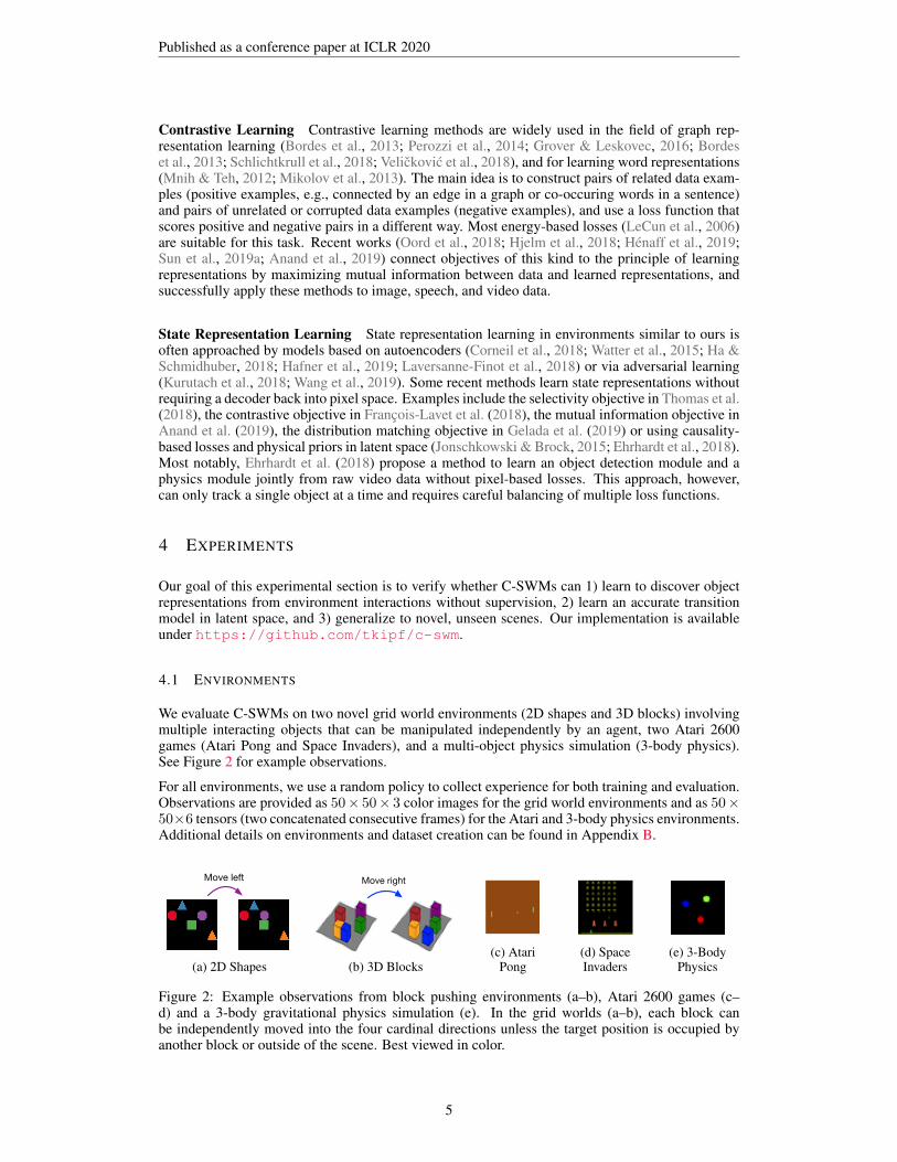
We evaluate C-SWMs on two novel grid world environments (2D shapes and 3D blocks) involvingmultiple interacting objects that can be manipulated independently by an agent, two Atari 2600games (Atari Pong and Space Invaders), and a multi-object physics simulation (3-body physics).See Figure 2 for example observations.

For all environments, we use a random policy to collect experience for both training and evaluation.Observations are provided as 50× 50× 3 color images for the grid world environments and as 50×50×6 tensors (two concatenated consecutive frames) for the Atari and 3-body physics environments.Additional details on environments and dataset creation can be found in Appendix B.

Move left Move right

(a) 2D Shapes

Move left Move right

(b) 3D Blocks(c) Atari

Pong(d) SpaceInvaders

(e) 3-BodyPhysics

Figure 2: Example observations from block pushing environments (a–b), Atari 2600 games (c–d) and a 3-body gravitational physics simulation (e). In the grid worlds (a–b), each block canbe independently moved into the four cardinal directions unless the target position is occupied byanother block or outside of the scene. Best viewed in color.

5

https://github.com/tkipf/c-swm


4.2 EVALUATION METRICS

In order to evaluate model performance directly in latent space, we make use of ranking metrics,which are commonly used for the evaluation of link prediction models, as in, e.g., Bordes et al.(2013). This allows us to assess the quality of learned representations directly without relying onauxiliary metrics such as pixel-based reconstruction losses, or performance in downstream taskssuch as planning.

Given an observation encoded by the model and an action, we use the model to predict the rep-resentation of the next state, reached after taking the action in the environment. This predictedstate representation is then compared to the encoded true observation after taking the action in theenvironment and a set of reference states (observations encoded by the model) obtained from theexperience buffer. We measure and report both Hits at Rank 1 (H@1) and Mean Reciprocal Rank(MRR). Additional details on these evaluation metrics can be found in Appendix C.

4.3 BASELINES

Autoencoder-based World Models The predominant method for state representation learning isbased on autoencoders, and often on the VAE (Kingma & Welling, 2013; Rezende et al., 2014)model in particular. This World Model baseline is inspired by Ha & Schmidhuber (2018) and useseither a deterministic autoencoder (AE) or a VAE to learn state representations. Finally, an MLP isused to predict the next state after taking an action.

Physics As Inverse Graphics (PAIG) This model by Jaques et al. (2019) is based on an encoder-decoder architecture and trained with pixel-based reconstruction losses, but uses a differentiablephysics engine in the latent space that operates on explicit position and velocity representations foreach object. Thus, this model is only applicable to the 3-body physics environment.

4.4 TRAINING AND EVALUATION SETTING

We train C-SWMs on an experience buffer obtained by running a random policy on the respectiveenvironment. We choose 1000 episodes with 100 environment steps each for the grid world envi-ronments, 1000 episodes with 10 steps each for the Atari environments and 5000 episodes with 10steps each for the 3-body physics environment.

For evaluation, we populate a separate experience buffer with 10 environment steps per episode anda total of 10.000 episodes for the grid world environments, 100 episodes for the Atari environmentsand 1000 episodes for the physics environment. For the Atari environments, we minimize train/testoverlap by ‘warm-starting’ experience collection in these environments with random actions beforewe start populating the experience buffer (see Appendix B), and we ensure that not a single fulltest set episode coincides exactly with an episode from the training set. The state spaces of thegrid world environments are large (approx. 6.4M unique states) and hence train/test coincidence ofa full 10-step episode is unlikely. Overlap is similarly unlikely for the physics environment whichhas a continuous state space. Hence, performing well on these tasks will require some form ofgeneralization to new environment configurations or an unseen sequence of states and actions.

All models are trained for 100 epochs (200 for Atari games) using the Adam (Kingma & Ba, 2014)optimizer with a learning rate of 5 · 10−4 and a batch size of 1024 (512 for baselines with decodersdue to higher memory demands, and 100 for PAIG as suggested by the authors). Model architecturedetails are provided in Appendix D.

4.5 QUALITATIVE RESULTS

We present qualitative results for the grid world environments in Figure 3 and for the 3-body physicsenvironment in Figure 4. All results are obtained on hold-out test data. Further qualitative results(incl. on Atari games) can be found in Appendix A.

In the grid world environments, we can observe that C-SWM reliably discovers object-specific fil-ters for a particular scene, without direct supervision. Further, each object is represented by twocoordinates which correspond (up to a random linear transformation) to the true object position in

6


(a) Discovered object masks in a scene from the 3Dcubes (top) and 2D shapes (bottom) environments.

(b) Learned abstract state transition graph of the yel-low cube (left) and the green square (right), whilekeeping all other object positions fixed at test time.

Figure 3: Discovered object masks (left) and direct visualization of the 2D abstract state spaces andtransition graphs for a single object (right) in the block pushing environments. Nodes denote stateembeddings obtained from a test set experience buffer with random actions and edges are predictedtransitions. The learned abstract state graph clearly captures the underlying grid structure of theenvironment both in terms of object-specific latent states and in terms of predicted transitions, butis randomly rotated and/or mirrored. The model further correctly captures that certain actions donot have an effect if a neighboring position is blocked by another object (shown as colored spheres),even though the transition model does not have access to visual inputs.

(a) Observations from 3-body gravitational physics simulation(bottom) and learned abstract state transition graph for a singleobject slot (top).

2.5 0.0 2.5

1

0

1

2

(b) Abstract state transition graph from50 test episodes for single object slot.

Figure 4: Qualitative results for 3-body physics environment for a single representative test setepisode (left) and for a dataset of 50 test episodes (right). The model learns to smoothly embed objecttrajectories, with the circular motion represented in the latent space (projected from four to twodimensions via PCA). In the abstract state transition graph, orange nodes denote starting states fora particular episode, green links correspond to ground truth transitions and violet links correspondto transitions predicted by the model. One trajectory (in the center) strongly deviates from typicaltrajectories seen during training, and the model struggles to predict the correct transition.

the scene. Although we choose a two-dimensional latent representation per object for easier vi-sualization, we find that results remain unchanged if we increase the dimensionality of the latentrepresentation. The edges in this learned abstract transition graph correspond to the effect of a par-ticular action applied to the object. The structure of the learned latent representation accuratelycaptures the underlying grid structure of the environment. We further find that the transition model,which only has access to latent representations, correctly captures whether an action has an effect ornot, e.g., if a neighboring position is blocked by another object.

Similarly, we find that the model can learn object-specific encoders in the 3-body physics envi-ronment and can learn object-specific latent representations that track location and velocity of aparticular object, while learning an accurate latent transition model that generalizes well to unseenenvironment instances.

4.6 QUANTITATIVE RESULTS

We set up quantitative experiments for evaluating the quality of both object discovery and the qualityof the learned transition model. We compare against autoencoder baselines and model variants thatdo not represent the environment in an object-factorized manner, do not use a GNN, or do not makeuse of contrastive learning. Performing well under this evaluation setting requires some degree of(combinatorial) generalization to unseen environment instances.

7


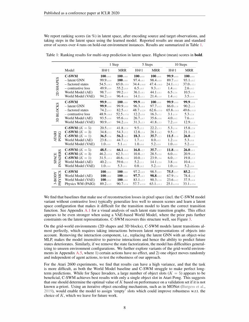
We report ranking scores (in %) in latent space, after encoding source and target observations, andtaking steps in the latent space using the learned model. Reported results are mean and standarderror of scores over 4 runs on hold-out environment instances. Results are summarized in Table 1.

Table 1: Ranking results for multi-step prediction in latent space. Highest (mean) scores in bold.

1 Step 5 Steps 10 Steps

Model H@1 MRR H@1 MRR H@1 MRR

2DSH

APE

S C-SWM 100±0.0 100±0.0 100±0.0 100±0.0 99.9±0.0 100±0.0

– latent GNN 99.9±0.0 100±0.0 97.4±0.1 98.4±0.0 89.7±0.3 93.1±0.2

– factored states 54.5±18.1 65.0±15.9 34.4±16.0 47.4±16.0 24.1±11.2 37.0±12.1

– contrastive loss 49.9±0.9 55.2±0.9 6.5±0.5 9.3±0.7 1.4±0.1 2.6±0.2

World Model (AE) 98.7±0.5 99.2±0.3 36.1±8.1 44.1±8.1 6.5±2.6 10.5±3.6

World Model (VAE) 94.2±1.0 96.4±0.6 14.1±1.1 21.4±1.4 1.4±0.2 3.5±0.4

3DB

LO

CK

S C-SWM 99.9±0.0 100±0.0 99.9±0.0 100±0.0 99.9±0.0 99.9±0.0

– latent GNN 99.9±0.0 99.9±0.0 96.3±0.4 97.7±0.3 86.0±1.8 90.2±1.5

– factored states 74.2±9.3 82.5±8.3 48.7±12.9 62.6±13.0 65.8±14.0 49.6±11.0

– contrastive loss 48.9±16.8 52.5±17.8 12.2±5.8 16.3±7.1 3.1±1.9 5.3±2.8

World Model (AE) 93.5±0.8 95.6±0.6 26.7±0.7 35.6±0.8 4.0±0.2 7.6±0.3

World Model (VAE) 90.9±0.7 94.2±0.6 31.3±2.3 41.8±2.3 7.2±0.9 12.9±1.3

ATA

RI

PON

G

C-SWM (K = 5) 20.5±3.5 41.8±2.9 9.5±2.2 22.2±3.3 5.3±1.6 15.8±2.8

C-SWM (K = 3) 34.8±5.3 54.3±5.2 12.8±3.4 28.1±4.2 9.5±1.7 21.1±2.8

C-SWM (K = 1) 36.5±5.6 56.2±6.2 18.3±1.9 35.7±2.3 11.5±1.0 26.0±1.2

World Model (AE) 23.8±3.3 44.7±2.4 1.7±0.5 8.0±0.5 1.2±0.8 5.3±0.8

World Model (VAE) 1.0±0.0 5.1±0.1 1.0±0.0 5.2±0.0 1.0±0.0 5.2±0.0

SPA

CE

INVA

DE

RS C-SWM (K = 5) 48.5±7.0 66.1±6.6 16.8±2.7 35.7±3.7 11.8±3.0 26.0±4.1

C-SWM (K = 3) 46.2±13.0 62.3±11.5 10.8±3.7 28.5±5.8 6.0±0.4 20.9±0.9

C-SWM (K = 1) 31.5±13.1 48.6±11.8 10.0±2.3 23.9±3.6 6.0±1.7 19.8±3.3

World Model (AE) 40.2±3.6 59.6±3.5 5.2±1.1 14.1±2.0 3.8±0.8 10.4±1.3

World Model (VAE) 1.0±0.0 5.3±0.1 0.8±0.2 5.2±0.0 1.0±0.0 5.2±0.0

3-B

OD

YPH

YSI

CS C-SWM 100±0.0 100±0.0 97.2±0.9 98.5±0.5 75.5±4.7 85.2±3.1

World Model (AE) 100±0.0 100±0.0 97.7±0.3 98.8±0.2 67.9±2.4 78.4±1.8

World Model (VAE) 100±0.0 100±0.0 83.1±2.5 90.3±1.6 23.6±4.2 37.5±4.8

Physics WM (PAIG) 89.2±3.5 90.7±3.4 57.7±12.0 63.1±11.1 25.1±13.0 33.1±13.4

We find that baselines that make use of reconstruction losses in pixel space (incl. the C-SWM modelvariant without contrastive loss) typically generalize less well to unseen scenes and learn a latentspace configuration that makes it difficult for the transition model to learn the correct transitionfunction. See Appendix A.1 for a visual analysis of such latent state transition graphs. This effectappears to be even stronger when using a VAE-based World Model, where the prior puts furtherconstraints on the latent representations. C-SWM recovers this structure well, see Figure 3.

On the grid-world environments (2D shapes and 3D blocks), C-SWM models latent transitions al-most perfectly, which requires taking interactions between latent representations of objects intoaccount. Removing the interaction component, i.e., replacing the latent GNN with an object-wiseMLP, makes the model insensitive to pairwise interactions and hence the ability to predict futurestates deteriorates. Similarly, if we remove the state factorization, the model has difficulties general-izing to unseen environment configurations. We further explore variants of the grid-world environ-ments in Appendix A.5, where 1) certain actions have no effect, and 2) one object moves randomlyand independent of agent actions, to test the robustness of our approach.

For the Atari 2600 experiments, we find that results can have a high variance, and that the taskis more difficult, as both the World Model baseline and C-SWM struggle to make perfect long-term predictions. While for Space Invaders, a large number of object slots (K = 5) appears to bebeneficial, C-SWM achieves best results with only a single object slot in Atari Pong. This suggeststhat one should determine the optimal value ofK based on performance on a validation set if it is notknown a-priori. Using an iterative object encoding mechanism, such as in MONet (Burgess et al.,2019), would enable the model to assign ‘empty’ slots which could improve robustness w.r.t. thechoice of K, which we leave for future work.

8


We find that both C-SWMs and the autoencoder-based World Model baseline excel at short-termpredictions in the 3-body physics environment, with C-SWM having a slight edge in the 10 step pre-diction setting. Under our evaluation setting, the PAIG baseline (Jaques et al., 2019) underperformsusing the hyperparameter setting recommended by the authors. Note that we do not tune hyperpa-rameters of C-SWM separately for this task and use the same settings as in other environments.

4.7 LIMITATIONS

Instance Disambiguation In our experiments, we chose a simple feed-forward CNN architecturefor the object extractor module. This type of architecture cannot disambiguate multiple instancesof the same object present in one scene and relies on distinct visual features or labels (e.g., thegreen square) for object extraction. To better handle scenes which contain potentially multiplecopies of the same object (e.g., in the Atari Space Invaders game), one would require some form ofiterative disambiguation procedure to break symmetries and dynamically bind individual objects toslots or object files (Kahneman & Treisman, 1984; Kahneman et al., 1992), such as in the style ofdynamic routing (Sabour et al., 2017), iterative inference (Greff et al., 2019; Engelcke et al., 2019)or sequential masking (Burgess et al., 2019; Kipf et al., 2019).

Stochasticity & Markov Assumption Our formulation of C-SWMs does not take into accountstochasticity in environment transitions or observations, and hence is limited to fully deterministicworlds. A probabilistic extension of C-SWMs is an interesting avenue for future work. For sim-plicity, we make the Markov assumption: state and action contain all the information necessary topredict the next state. This allows us to look at single state-action-state triples in isolation. To gobeyond this limitation, one would require some form of memory mechanism, such as an RNN aspart of the model architecture, which we leave for future work.

5 CONCLUSIONS

Structured world models offer compelling advantages over pure connectionist methods, by enablingstronger inductive biases for generalization, without necessarily constraining the generality of themodel: for example, the contrastively trained model on the 3-body physics environment is free tostore identical representations in each object slot and ignore pairwise interactions, i.e., an unstruc-tured world model still exists as a special case. Experimentally, we find that C-SWMs make effectiveuse of this additional structure, likely because it allows for a transition model of significantly lowercomplexity, and learn object-oriented models that generalize better to unseen situations.

We are excited about the prospect of using C-SWMs for model-based planning and reinforcementlearning in future work, where object-oriented representations will likely allow for more accuratecounterfactual reasoning about effects of actions and novel interactions in the environment. Wefurther hope to inspire future work to think beyond autoencoder-based approaches for object-based,structured representation learning, and to address some of the limitations outlined in this paper.

ACKNOWLEDGEMENTS

We would like to thank Marco Federici and Adam Kosiorek for helpful discussions. We wouldfurther like to thank the anonymous reviewers for valuable feedback. T.K. acknowledges funding bySAP SE.

REFERENCES

Ankesh Anand, Evan Racah, Sherjil Ozair, Yoshua Bengio, Marc-Alexandre Cote, and R DevonHjelm. Unsupervised state representation learning in Atari. arXiv preprint arXiv:1906.08226,2019.

Jimmy Lei Ba, Jamie Ryan Kiros, and Geoffrey E Hinton. Layer normalization. arXiv preprintarXiv:1607.06450, 2016.

Peter Battaglia, Razvan Pascanu, Matthew Lai, Danilo Jimenez Rezende, et al. Interaction networksfor learning about objects, relations and physics. In NIPS, 2016.

9


Peter W Battaglia, Jessica B Hamrick, Victor Bapst, Alvaro Sanchez-Gonzalez, Vinicius Zambaldi,Mateusz Malinowski, Andrea Tacchetti, David Raposo, Adam Santoro, Ryan Faulkner, et al.Relational inductive biases, deep learning, and graph networks. arXiv preprint arXiv:1806.01261,2018.

Marc G Bellemare, Yavar Naddaf, Joel Veness, and Michael Bowling. The arcade learning envi-ronment: An evaluation platform for general agents. Journal of Artificial Intelligence Research,2013.

Antoine Bordes, Nicolas Usunier, Alberto Garcia-Duran, Jason Weston, and Oksana Yakhnenko.Translating embeddings for modeling multi-relational data. In NIPS, 2013.

Greg Brockman, Vicki Cheung, Ludwig Pettersson, Jonas Schneider, John Schulman, Jie Tang, andWojciech Zaremba. Openai gym. arXiv preprint arXiv:1606.01540, 2016.

Christopher P Burgess, Loic Matthey, Nicholas Watters, Rishabh Kabra, Irina Higgins, MattBotvinick, and Alexander Lerchner. Monet: Unsupervised scene decomposition and represen-tation. arXiv preprint arXiv:1901.11390, 2019.

Michael B Chang, Tomer Ullman, Antonio Torralba, and Joshua B Tenenbaum. A compositionalobject-based approach to learning physical dynamics. arXiv preprint arXiv:1612.00341, 2016.

Dane Corneil, Wulfram Gerstner, and Johanni Brea. Efficient model-based deep reinforcementlearning with variational state tabulation. arXiv preprint arXiv:1802.04325, 2018.

Sebastien Ehrhardt, Aron Monszpart, Niloy Mitra, and Andrea Vedaldi. Unsupervised intuitivephysics from visual observations. In Asian Conference on Computer Vision. Springer, 2018.

Martin Engelcke, Adam R Kosiorek, Oiwi Parker Jones, and Ingmar Posner. Genesis: Gener-ative scene inference and sampling with object-centric latent representations. arXiv preprintarXiv:1907.13052, 2019.

SM Ali Eslami, Nicolas Heess, Theophane Weber, Yuval Tassa, David Szepesvari, KorayKavukcuoglu, and Geoffrey E Hinton. Attend, infer, repeat: Fast scene understanding with gen-erative models. In NIPS, 2016.

Vincent Francois-Lavet, Yoshua Bengio, Doina Precup, and Joelle Pineau. Combined reinforcementlearning via abstract representations. arXiv preprint arXiv:1809.04506, 2018.

Carles Gelada, Saurabh Kumar, Jacob Buckman, Ofir Nachum, and Marc G Bellemare. Deep-MDP: Learning continuous latent space models for representation learning. arXiv preprintarXiv:1906.02736, 2019.

Justin Gilmer, Samuel S Schoenholz, Patrick F Riley, Oriol Vinyals, and George E Dahl. Neuralmessage passing for quantum chemistry. In ICML, 2017.

Klaus Greff, Sjoerd van Steenkiste, and Jurgen Schmidhuber. Neural expectation maximization. InNIPS, 2017.

Klaus Greff, Raphael Lopez Kaufmann, Rishab Kabra, Nick Watters, Chris Burgess, Daniel Zoran,Loic Matthey, Matthew Botvinick, and Alexander Lerchner. Multi-object representation learningwith iterative variational inference. arXiv preprint arXiv:1903.00450, 2019.

Aditya Grover and Jure Leskovec. node2vec: Scalable feature learning for networks. In KDD, 2016.

David Ha and Jurgen Schmidhuber. World models. arXiv preprint arXiv:1803.10122, 2018.

Danijar Hafner, Timothy Lillicrap, Ian Fischer, Ruben Villegas, David Ha, Honglak Lee, and JamesDavidson. Learning latent dynamics for planning from pixels. In ICML, 2019.

Olivier J Henaff, Ali Razavi, Carl Doersch, SM Eslami, and Aaron van den Oord. Data-efficientimage recognition with contrastive predictive coding. arXiv preprint arXiv:1905.09272, 2019.

10


R Devon Hjelm, Alex Fedorov, Samuel Lavoie-Marchildon, Karan Grewal, Adam Trischler, andYoshua Bengio. Learning deep representations by mutual information estimation and maximiza-tion. arXiv preprint arXiv:1808.06670, 2018.

Yedid Hoshen. Vain: Attentional multi-agent predictive modeling. In NIPS, 2017.

John D Hunter. Matplotlib: A 2d graphics environment. Computing In Science & Engineering,2007.

Sergey Ioffe and Christian Szegedy. Batch normalization: Accelerating deep network training byreducing internal covariate shift. arXiv preprint arXiv:1502.03167, 2015.

Michael Janner, Sergey Levine, William T Freeman, Joshua B Tenenbaum, Chelsea Finn, and JiajunWu. Reasoning about physical interactions with object-oriented prediction and planning. In ICLR,2019.

Miguel Jaques, Michael Burke, and Timothy Hospedales. Physics-as-inverse-graphics: Joint unsu-pervised learning of objects and physics from video. arXiv preprint arXiv:1905.11169, 2019.

Rico Jonschkowski and Oliver Brock. Learning state representations with robotic priors. Au-tonomous Robots, 2015.

Daniel Kahneman and Anne Treisman. Changing views of Attention and Automaticity. AcademicPress, Inc., San Diego, CA, 1984.

Daniel Kahneman, Anne Treisman, and Brian J Gibbs. The reviewing of object files: Object-specificintegration of information. Cognitive psychology, 1992.

Lukasz Kaiser, Mohammad Babaeizadeh, Piotr Milos, Blazej Osinski, Roy H Campbell, KonradCzechowski, Dumitru Erhan, Chelsea Finn, Piotr Kozakowski, Sergey Levine, et al. Model-basedreinforcement learning for atari. arXiv preprint arXiv:1903.00374, 2019.

Diederik P Kingma and Jimmy Ba. Adam: A method for stochastic optimization. arXiv preprintarXiv:1412.6980, 2014.

Diederik P Kingma and Max Welling. Auto-encoding variational bayes. arXiv preprintarXiv:1312.6114, 2013.

Thomas Kipf, Ethan Fetaya, Kuan-Chieh Wang, Max Welling, and Richard Zemel. Neural relationalinference for interacting systems. In ICML, 2018.

Thomas Kipf, Yujia Li, Hanjun Dai, Vinicius Zambaldi, Alvaro Sanchez-Gonzalez, Edward Grefen-stette, Pushmeet Kohli, and Peter Battaglia. Compile: Compositional imitation learning andexecution. In ICML, 2019.

Thomas N Kipf and Max Welling. Semi-supervised classification with graph convolutional net-works. arXiv preprint arXiv:1609.02907, 2016.

Adam Kosiorek, Hyunjik Kim, Yee Whye Teh, and Ingmar Posner. Sequential attend, infer, repeat:Generative modelling of moving objects. In NeurIPS, 2018.

Thanard Kurutach, Aviv Tamar, Ge Yang, Stuart J Russell, and Pieter Abbeel. Learning plannablerepresentations with causal infogan. In NeurIPS, 2018.

Adrien Laversanne-Finot, Alexandre Pere, and Pierre-Yves Oudeyer. Curiosity driven explorationof learned disentangled goal spaces. arXiv preprint arXiv:1807.01521, 2018.

Yann LeCun, Sumit Chopra, Raia Hadsell, M Ranzato, and F Huang. A tutorial on energy-basedlearning. Predicting structured data, 2006.

Yujia Li, Daniel Tarlow, Marc Brockschmidt, and Richard Zemel. Gated graph sequence neuralnetworks. arXiv preprint arXiv:1511.05493, 2015.

Long-Ji Lin. Self-improving reactive agents based on reinforcement learning, planning and teaching.Machine learning, 8(3-4):293–321, 1992.

11


Tomas Mikolov, Kai Chen, Greg Corrado, and Jeffrey Dean. Efficient estimation of word represen-tations in vector space. arXiv preprint arXiv:1301.3781, 2013.

Andriy Mnih and Yee Whye Teh. A fast and simple algorithm for training neural probabilisticlanguage models. arXiv preprint arXiv:1206.6426, 2012.

Charlie Nash, Ali Eslami, Chris Burgess, Irina Higgins, Daniel Zoran, Theophane Weber, and PeterBattaglia. The multi-entity variational autoencoder. In NIPS Workshops, 2017.

Maximilian Nickel, Volker Tresp, and Hans-Peter Kriegel. A three-way model for collective learningon multi-relational data. In ICML, 2011.

Maximilian Nickel, Kevin Murphy, Volker Tresp, and Evgeniy Gabrilovich. A review of relationalmachine learning for knowledge graphs. Proceedings of the IEEE, 2016a.

Maximilian Nickel, Lorenzo Rosasco, and Tomaso Poggio. Holographic embeddings of knowledgegraphs. In AAAI, 2016b.

Aaron van den Oord, Yazhe Li, and Oriol Vinyals. Representation learning with contrastive predic-tive coding. arXiv preprint arXiv:1807.03748, 2018.

Bryan Perozzi, Rami Al-Rfou, and Steven Skiena. Deepwalk: Online learning of social representa-tions. In KDD, 2014.

Danilo Jimenez Rezende, Shakir Mohamed, and Daan Wierstra. Stochastic backpropagation andapproximate inference in deep generative models. arXiv preprint arXiv:1401.4082, 2014.

Sara Sabour, Nicholas Frosst, and Geoffrey E Hinton. Dynamic routing between capsules. In NIPS,2017.

Alvaro Sanchez-Gonzalez, Nicolas Heess, Jost Tobias Springenberg, Josh Merel, Martin Riedmiller,Raia Hadsell, and Peter Battaglia. Graph networks as learnable physics engines for inference andcontrol. In ICML, 2018.

Franco Scarselli, Marco Gori, Ah Chung Tsoi, Markus Hagenbuchner, and Gabriele Monfardini.The graph neural network model. IEEE Transactions on Neural Networks, 2009.

Michael Schlichtkrull, Thomas N Kipf, Peter Bloem, Rianne Van Den Berg, Ivan Titov, and MaxWelling. Modeling relational data with graph convolutional networks. In ESWC, 2018.

Elizabeth S Spelke and Katherine D Kinzler. Core knowledge. Developmental science, 2007.

Sainbayar Sukhbaatar, Rob Fergus, et al. Learning multiagent communication with backpropaga-tion. In NIPS, 2016.

Chen Sun, Abhinav Shrivastava, Carl Vondrick, Kevin Murphy, Rahul Sukthankar, and CordeliaSchmid. Actor-centric relation network. In ECCV, 2018.

Chen Sun, Fabien Baradel, Kevin Murphy, and Cordelia Schmid. Contrastive bidirectional trans-former for temporal representation learning. arXiv preprint arXiv:1906.05743, 2019a.

Chen Sun, Abhinav Shrivastava, Carl Vondrick, Rahul Sukthankar, Kevin Murphy, and CordeliaSchmid. Relational action forecasting. arXiv preprint arXiv:1904.04231, 2019b.

Valentin Thomas, Emmanuel Bengio, William Fedus, Jules Pondard, Philippe Beaudoin, HugoLarochelle, Joelle Pineau, Doina Precup, and Yoshua Bengio. Disentangling the independentlycontrollable factors of variation by interacting with the world. arXiv preprint arXiv:1802.09484,2018.

Theo Trouillon, Johannes Welbl, Sebastian Riedel, Eric Gaussier, and Guillaume Bouchard. Com-plex embeddings for simple link prediction. In ICML, 2016.

Sjoerd van Steenkiste, Michael Chang, Klaus Greff, and Jurgen Schmidhuber. Relational neural ex-pectation maximization: Unsupervised discovery of objects and their interactions. arXiv preprintarXiv:1802.10353, 2018.

12


Petar Velickovic, William Fedus, William L Hamilton, Pietro Lio, Yoshua Bengio, and R DevonHjelm. Deep graph infomax. arXiv preprint arXiv:1809.10341, 2018.

Angelina Wang, Thanard Kurutach, Kara Liu, Pieter Abbeel, and Aviv Tamar. Learning roboticmanipulation through visual planning and acting. arXiv preprint arXiv:1905.04411, 2019.

Tingwu Wang, Renjie Liao, Jimmy Ba, and Sanja Fidler. Nervenet: Learning structured policy withgraph neural networks. In ICLR, 2018.

Zhen Wang, Jianwen Zhang, Jianlin Feng, and Zheng Chen. Knowledge graph embedding by trans-lating on hyperplanes. In AAAI, 2014.

Manuel Watter, Jost Springenberg, Joschka Boedecker, and Martin Riedmiller. Embed to control: Alocally linear latent dynamics model for control from raw images. In NIPS, 2015.

Nicholas Watters, Daniel Zoran, Theophane Weber, Peter Battaglia, Razvan Pascanu, and AndreaTacchetti. Visual interaction networks: Learning a physics simulator from video. In NIPS, 2017.

Nicholas Watters, Loic Matthey, Matko Bosnjak, Christopher P Burgess, and Alexander Lerchner.Cobra: Data-efficient model-based rl through unsupervised object discovery and curiosity-drivenexploration. arXiv preprint arXiv:1905.09275, 2019.

Bing Xu, Naiyan Wang, Tianqi Chen, and Mu Li. Empirical evaluation of rectified activations inconvolutional network. arXiv preprint arXiv:1505.00853, 2015.

Zhenjia Xu, Zhijian Liu, Chen Sun, Kevin Murphy, William T Freeman, Joshua B Tenenbaum,and Jiajun Wu. Unsupervised discovery of parts, structure, and dynamics. arXiv preprintarXiv:1903.05136, 2019.

13


A ADDITIONAL RESULTS AND DISCUSSION

A.1 OBJECT-SPECIFIC REPRESENTATIONS

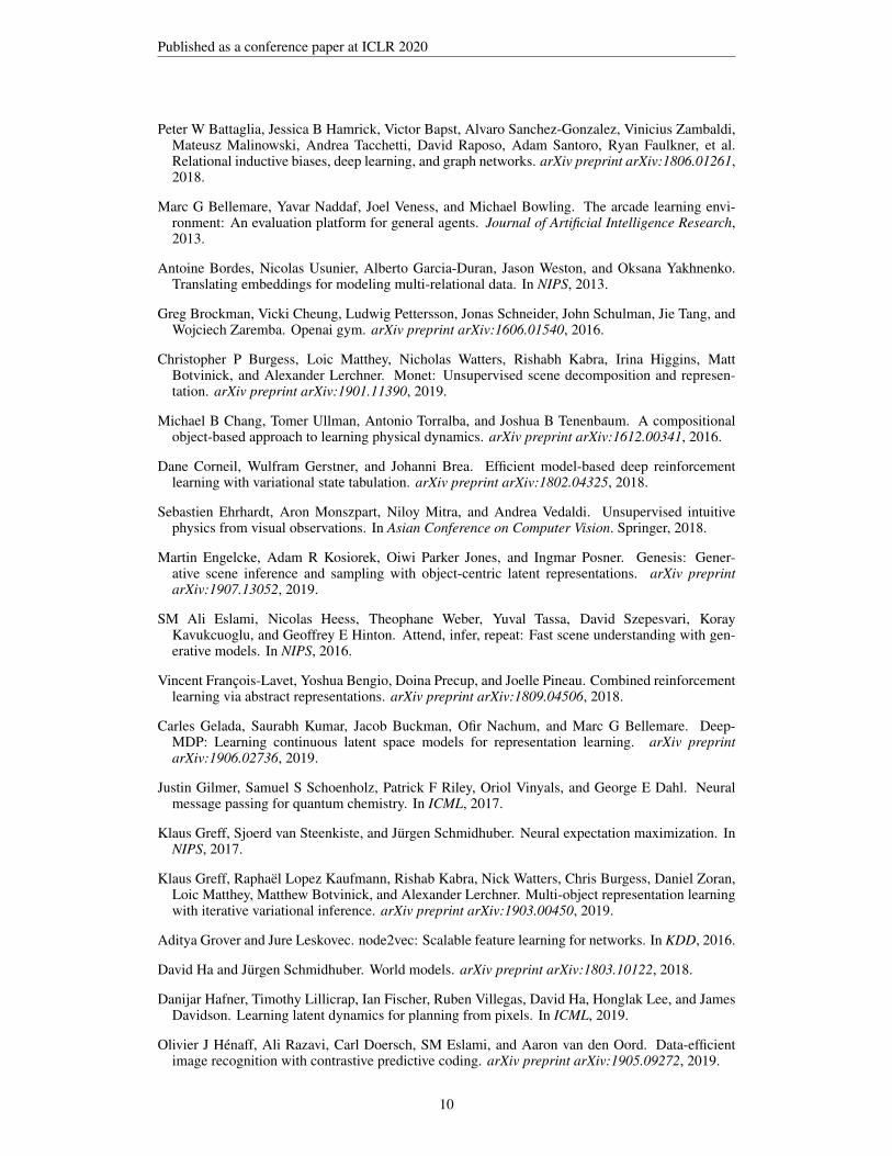
We visualize abstract state transition graphs separated by object slot for the 3D cubes environmentin Figure 5. Discovered object representations in the 2D shapes dataset (not shown) are qualitativelyvery similar. We apply the same visualization technique to the model variant without contrastiveloss, which is instead trained with a decoder model and a loss in pixel space. See Figure 6 for thisbaseline and note that the regular structure in the latent space is lost, which makes it difficult for thetransition model to learn transitions which generalize to unseen environment instances.

Qualitative results for the 3-body physics dataset are summarized in Figures 7 and 8 for two differentrandom seeds.

(a) Object slot 1. (b) Object slot 2. (c) Object slot 3. (d) Object slot 4. (e) Object slot 5.

Figure 5: Abstract state transition graphs per object slot for a trained C-SWM model on the 3Dcubes environment (with all objects allowed to be moved, i.e., none are fixed in place). Edge colordenotes action type. The abstract state graph is nearly identical for each object, which illustrates thatthe model successfully represents objects in the same manner despite their visual differences.

(a) Object slot 1. (b) Object slot 2. (c) Object slot 3. (d) Object slot 4. (e) Object slot 5.

Figure 6: Abstract state transition graphs per object slot for a trained SWM model without con-trastive loss, using instead a loss in pixel space, on the 3D cubes environment. Edge color denotesaction type.

(a) Discovered object-specific filters.2.5 0.0 2.5

2

1

0

1

2

(b) Object slot 1.2.5 0.0 2.5

2

0

2

(c) Object slot 2.2.5 0.0 2.5

1

0

1

2

(d) Object slot 3.

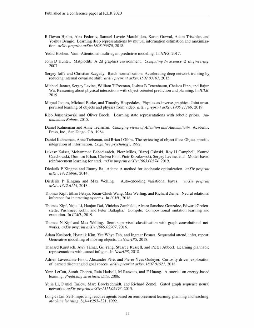
Figure 7: Object filters (left) and abstract state transition graphs per object slot (right) for a trainedC-SWM model on unseen test instances of the 3-body physics environment (seed 1).

For the Atari 2600 environments, we generally found latent object representations to be less in-terpretable. We attribute this to the fact that a) objects have different roles and are in general notexchangeable (in contrast to the block pushing grid world environments and the 3-body physicsenvironment), b) actions affect only one object directly, but many other objects indirectly in twoconsecutive frames, and c) due to multiple objects in one scene sharing the same visual features.See Figure 9 for an example of learned representations in Atari Pong and Figure 10 for an examplein Space Invaders.

14


(a) Discovered object-specific filters.2 0 2

2

1

0

1

2

(b) Object slot 1.2 0 2

2

1

0

1

2

(c) Object slot 2.2 0 2

2

1

0

1

2

(d) Object slot 3.

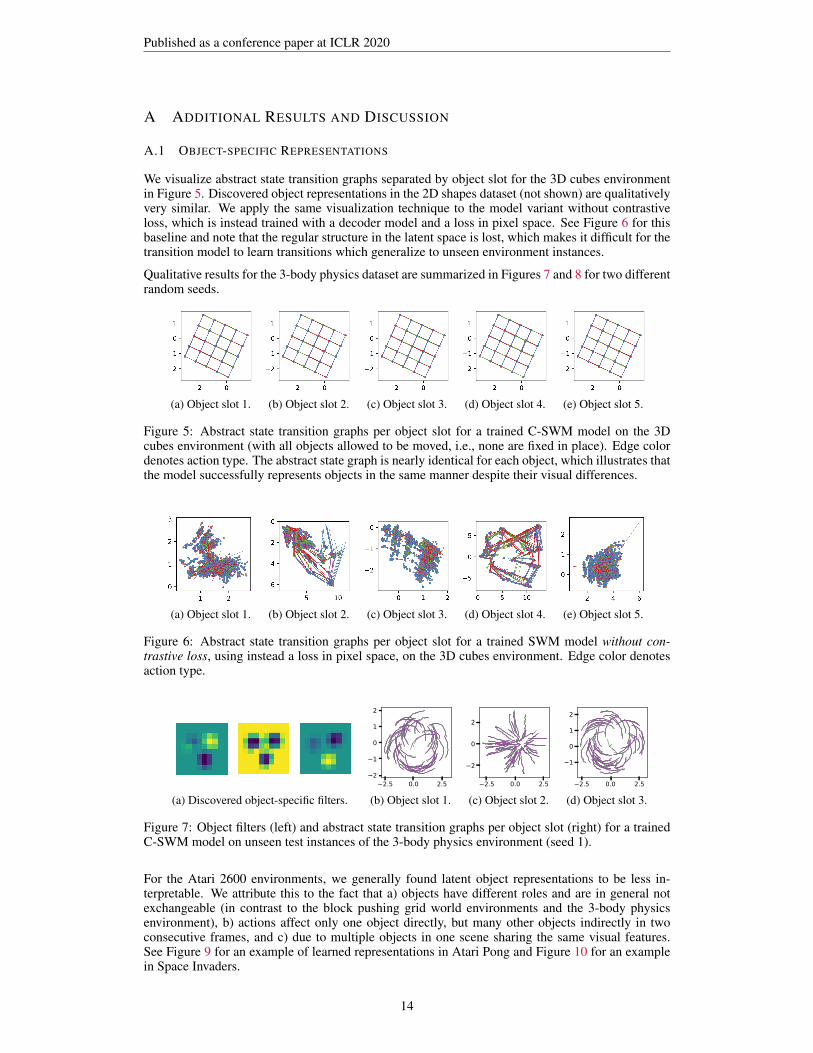
Figure 8: Object filters (left) and abstract state transition graphs per object slot (right) for a trainedC-SWM model on unseen test instances of the 3-body physics environment (seed 2).


1

0

1

(b) Object slot 1.2.5 0.0 2.5

2

0

2


1

0

1

(d) Object slot 3.

Figure 9: Object filters (left) and abstract state transition graphs per object slot (right) for a trainedC-SWM model with K = 3 object slots on unseen test instances of the Atari Pong environment.


0.05

0.00

0.05

0.10

(b) Object slot 1.2.5 0.0 2.5

0.0

0.5

1.0


2

0

2

(d) Object slot 3.

Figure 10: Object filters (left) and abstract state transition graphs per object slot (right) for a trainedC-SWM model withK = 3 object slots on unseen test instances of the Space Invaders environment.

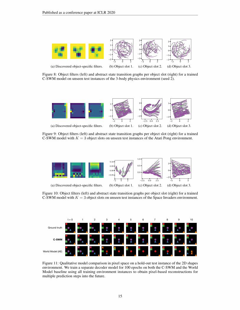
Ground truth

C-SWM

World Model (AE)

t = 0 1 2 3 4 5 6 7 8 9 10

Figure 11: Qualitative model comparison in pixel space on a hold-out test instance of the 2D shapesenvironment. We train a separate decoder model for 100 epochs on both the C-SWM and the WorldModel baseline using all training environment instances to obtain pixel-based reconstructions formultiple prediction steps into the future.

15


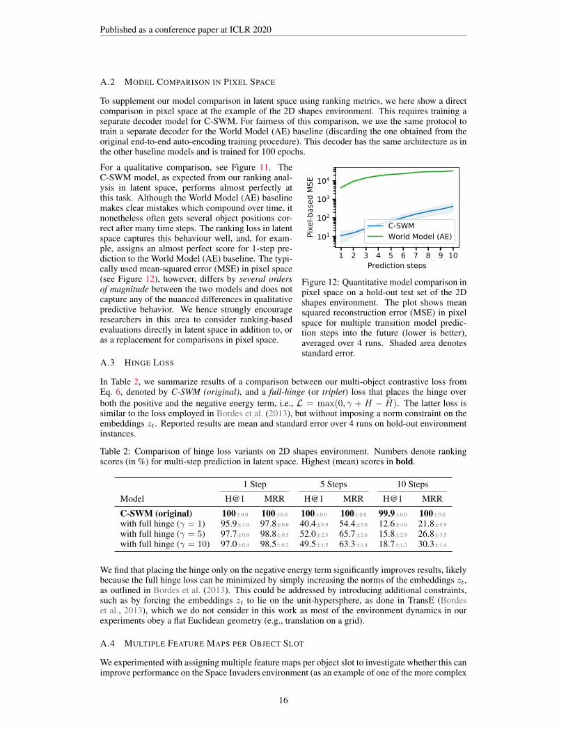
A.2 MODEL COMPARISON IN PIXEL SPACE

To supplement our model comparison in latent space using ranking metrics, we here show a directcomparison in pixel space at the example of the 2D shapes environment. This requires training aseparate decoder model for C-SWM. For fairness of this comparison, we use the same protocol totrain a separate decoder for the World Model (AE) baseline (discarding the one obtained from theoriginal end-to-end auto-encoding training procedure). This decoder has the same architecture as inthe other baseline models and is trained for 100 epochs.

1 2 3 4 5 6 7 8 9 10Prediction steps

101

102

103

104

Pixe

l-bas

ed M

SE

C-SWMWorld Model (AE)

Figure 12: Quantitative model comparison inpixel space on a hold-out test set of the 2Dshapes environment. The plot shows meansquared reconstruction error (MSE) in pixelspace for multiple transition model predic-tion steps into the future (lower is better),averaged over 4 runs. Shaded area denotesstandard error.

For a qualitative comparison, see Figure 11. TheC-SWM model, as expected from our ranking anal-ysis in latent space, performs almost perfectly atthis task. Although the World Model (AE) baselinemakes clear mistakes which compound over time, itnonetheless often gets several object positions cor-rect after many time steps. The ranking loss in latentspace captures this behaviour well, and, for exam-ple, assigns an almost perfect score for 1-step pre-diction to the World Model (AE) baseline. The typi-cally used mean-squared error (MSE) in pixel space(see Figure 12), however, differs by several ordersof magnitude between the two models and does notcapture any of the nuanced differences in qualitativepredictive behavior. We hence strongly encourageresearchers in this area to consider ranking-basedevaluations directly in latent space in addition to, oras a replacement for comparisons in pixel space.

A.3 HINGE LOSS

In Table 2, we summarize results of a comparison between our multi-object contrastive loss fromEq. 6, denoted by C-SWM (original), and a full-hinge (or triplet) loss that places the hinge overboth the positive and the negative energy term, i.e., L = max(0, γ + H − H). The latter loss issimilar to the loss employed in Bordes et al. (2013), but without imposing a norm constraint on theembeddings zt. Reported results are mean and standard error over 4 runs on hold-out environmentinstances.

Table 2: Comparison of hinge loss variants on 2D shapes environment. Numbers denote rankingscores (in %) for multi-step prediction in latent space. Highest (mean) scores in bold.



C-SWM (original) 100±0.0 100±0.0 100±0.0 100±0.0 99.9±0.0 100±0.0

with full hinge (γ = 1) 95.9±1.0 97.8±0.6 40.4±5.9 54.4±5.8 12.6±4.0 21.8±5.9

with full hinge (γ = 5) 97.7±0.9 98.8±0.5 52.0±2.5 65.7±2.6 15.8±2.9 26.8±3.5

with full hinge (γ = 10) 97.0±0.4 98.5±0.2 49.5±1.5 63.3±1.4 18.7±1.2 30.3±1.4

We find that placing the hinge only on the negative energy term significantly improves results, likelybecause the full hinge loss can be minimized by simply increasing the norms of the embeddings zt,as outlined in Bordes et al. (2013). This could be addressed by introducing additional constraints,such as by forcing the embeddings zt to lie on the unit-hypersphere, as done in TransE (Bordeset al., 2013), which we do not consider in this work as most of the environment dynamics in ourexperiments obey a flat Euclidean geometry (e.g., translation on a grid).

A.4 MULTIPLE FEATURE MAPS PER OBJECT SLOT

We experimented with assigning multiple feature maps per object slot to investigate whether this canimprove performance on the Space Invaders environment (as an example of one of the more complex

16


environments considered in this work). All other model settings are left unchanged. Results aresummarized in Table 3. The original model variant with one feature map per object slot (using atotal of K = 5 slots) is denoted by C-SWM (original). Reported results are mean and standard errorover 4 runs on hold-out environment instances.

Table 3: Comparison of model variants with multiple feature maps per object on the Space Invadersenvironment. Numbers denote ranking scores (in %) for multi-step prediction in latent space.



C-SWM (original) 48.5±7.0 66.1±6.6 16.8±2.7 35.7±3.7 11.8±3.0 26.0±4.1

with 2 feature maps 48.2±7.1 65.7±6.8 12.8±3.0 27.7±3.2 8.2±2.9 21.2±3.4



We find that there is no clear advantage in using multiple feature maps per object slot for the SpaceInvaders environment, but this might nonetheless prove useful for environments of more complexnature.

A.5 GRID-WORLD ENVIRONMENT VARIANTS

To further evaluate the robustness of our approach, we experimented with two variants of the 2Dshapes grid-world environment with five objects. In the first variant, termed no-op action, we includean additional ‘no-op’ action for each object that has no effect. This mirrors the setting present inmany Atari 2600 benchmark environments that have an explicit no-op action. In the second variant,termed random object, we assign a special property to one out of the five objects: a random action isapplied to this object at every turn, i.e., the agent only has control over the other four objects and inevery environment step, a total of two objects receive an action (one by the agent, which only affectsone out of the first four objects, and one random action on the last object). This is to test how themodel behaves in the presence of other agents that act randomly. As our model is fully deterministic,it is to be expected that adding a source of randomness in the environment will pose a challenge.

We report results in Table 4. Reported numbers are mean and standard error over 4 runs on hold-outenvironment instances. We find that adding a no-op action has little effect on our model, but addinga randomly moving object reduces predictive performance. Performance in the latter case couldpotentially be improved by explicitly modeling stochasticity in the environment.

Table 4: Comparison of C-SWM on variants of the 2D shapes environment. Numbers denote rankingscores (in %) for multi-step prediction in latent space.



C-SWM (original env.) 100±0.0 100±0.0 100±0.0 100±0.0 99.9±0.0 100±0.0

+ no-op action 100±0.0 100±0.0 100±0.0 100±0.0 99.9±0.0 99.9±0.0

+ random object 98.4±0.1 99.2±0.0 95.9±0.2 97.6±0.1 90.4±0.3 93.7±0.2

A.6 STABILITY

The discovered object representations and identifications can vary between runs. While we foundthat this process is very stable for the simple grid world environments where actions only affect asingle object, we found that results can be initialization-dependent on the Atari environments, whereactions can have effects across all objects, and the 3-body physics simulation (see Figures 7 and 8),which does not have any actions. In some cases, the discovered representation can be less suitablefor forward prediction in time or for generalization to novel scenes, which explains the variance insome of our results on these datasets.

17


A.7 TRAINING TIME

We found that the overall training time of the C-SWM model was comparable to that of the WorldModel baseline. Both C-SWM and the World Model baseline trained for approx. 1 hour wall-clocktime on the 2D shapes dataset, approx. 2 hours on the 3D cubes dataset, and approx. 30min on the3-body physics environment using a single NVIDIA GTX1080Ti GPU. The Atari Pong and SpaceInvaders models trained for typically less than 20 minutes. A notable exception is the PAIG baselinemodel (Jaques et al., 2019) which trained for approx. 6 hours on a NVIDIA TitanX Pascal GPUusing the recommended settings by the authors of the paper.

B DATASETS

B.1 GRID WORLDS

To generate an experience buffer for training, we initialize the environment with random objectplacements and uniformly sample an object and an object-specific action at every time step.

We provide state observations as 50× 50× 3 tensors with RGB color channels, normalized to [0, 1].Actions are provided as a 4-dim one-hot vector (if an action is applied) or a vector of zeros per objectslot in the environment. The action one-hot vector encodes the directional movement action appliedto a particular object, or is represented as a vector of zeros if no action is applied to a particularobject. Note that only a single object receives an action per time step. For the Atari environments,we provide a copy of the one-hot encoded action vector to every object slot, and for the 3-bodyphysics environment, which has no actions, we do not provide an action vector.

2D Shapes This environment is a 5 × 5 grid world with 5 different objects placed at randompositions. Each location can only be occupied by at maximum one object. Each object is representedby a unique shape/color combination, occupying 10 × 10 pixels on the overall 50 × 50 pixel grid.At each time step, one object can be selected and moved by one position along the four cardinaldirections. See Figure 2a for an example. The action has no effect if the target location in a particulardirection is occupied by another object or outside of the 5× 5 grid. Thus, a learned transition modelneeds to take pairwise interactions between object properties (i.e., their locations) into account, as itwould otherwise be unable to predict the effect of an action correctly.

3D Blocks To investigate to what degree our model is robust to partial occlusion and perspectivechanges, we implement a simple block pushing environment using Matplotlib (Hunter, 2007) as arendering tool. The underlying environment dynamics are the same as in the 2D Shapes dataset, andwe only change the rendering component to make for a visually more challenging task that involvesa different perspective and partial occlusions. See Figure 2b for an example.

B.2 ATARI 2600 GAMES

Atari Pong We make use of the Arcade Learning Environment (Bellemare et al., 2013) to createa small environment based on the Atari 2600 game Pong which is restricted to the first interactionbetween the ball and the player-controlled paddle, i.e., we discard the first couple of frames from theexperience buffer where the opponent behaves completely independent of any player action. Specifi-cally, we discard the first 58 (random) environment interactions. We use the PONGDETERMINISTIC-V4 variant of the environment in OpenAI Gym (Brockman et al., 2016). We use a random policyand populate an experience buffer with 10 environment interactions per episode, i.e., T = 10. Anobservation consists of two consecutive frames, cropped (to exclude the score) and resized to 50×50pixels each. See Figure 2c for an example.

Space Invaders This environment is based on the Atari 2600 game Space Invaders, using theSPACEINVADERSDETERMINISTIC-V4 variant of the environment in OpenAI Gym (Brockmanet al., 2016), and processed / restricted in a similar manner as the Pong environment. We dis-card the first 50 (random) environment interactions for each episode and only begin populating theexperience buffer thereafter. See Figure 2d for an example observation.

18


B.3 3-BODY PHYSICS

The 3-body physics simulation environment is an interacting system that evolves according to clas-sical gravitational dynamics. Different from the other environments considered here, there are noactions. This environment is adapted from Jaques et al. (2019) using their publicly available imple-mentation1, where we set the step size (dt) to 2.0 and the initial maximum x and y velocities to 0.5.We concatenate two consecutive frames of 50× 50 pixels each to provide the model with (implicit)velocity information. See Figure 4 for an example observation sequence.

C EVALUATION METRICS

C.1 HITS AT RANK K (H@K)

This score is 1 for a particular example if the predicted state representation is in the k-nearest neigh-bor set around the encoded true observation, where we define the neighborhood of a node to includethe node itself. Otherwise this score is 0. In other words, this score measures whether the rankof the predicted state representation is smaller than or equal to k, when ranking all reference staterepresentations by distance to the true state representation. We report the average of this score overa particular evaluation dataset.

C.2 MEAN RECIPROCAL RANK (MRR)

This score is defined as the average inverse rank, i.e., MRR = 1N

∑Nn=1

1rankn

, where rankn is therank of the n-th sample.

D ARCHITECTURE AND HYPERPARAMETERS

D.1 OBJECT EXTRACTOR

For the 3D cubes environment, the object extractor is a 4-layer CNN with 3×3 filters, zero-padding,and 16 feature maps per layer, with the exception of the last layer, which has K = 5 feature maps,i.e., one per object slot. After each layer, we apply BatchNorm (Ioffe & Szegedy, 2015) and aReLU(x) = max(0, x) activation function. For the 2D shapes environment, we choose a simplerCNN architecture with only a single convolutional layer with 10 × 10 filters and a stride of 10,followed by BatchNorm and a ReLU activation or LeakyReLU (Xu et al., 2015) for the Atari 2600and physics environments. This layer has 16 feature maps and is followed by a channel-wise lineartransformation (i.e., a 1 × 1 convolution), with 5 feature maps as output. For both models, wechoose a sigmoid activation function after the last layer to obtain object masks with values in (0, 1).We use the same two-layer architecture for the Atari 2600 environments and the 3-body physicsenvironment, but with 9× 9 filters (and zero-padding) in the first layer, and 5× 5 filters with a strideof 5 in the second layer.

D.2 OBJECT ENCODER

After reshaping/flattening the output of the object extractor, we obtain a vector representation perobject (2500-dim for the 3D cubes environment, 25-dim for the 2D shapes environment, and 1000-dim for Atari 2600 and physics environments). The object encoder is an MLP with two hiddenlayers of 512 units and each, followed by ReLU activation functions. We further use LayerNorm(Ba et al., 2016) before the activation function of the second hidden layer. The output of the finaloutput layer is 2-dimensional (4-dimensional for Atari 2600 and physics environments), reflectingthe ground truth object state, i.e., the object coordinates in 2D (although this is not provided to themodel), and velocity (if applicable).

1https://github.com/seuqaj114/paig

19

https://github.com/seuqaj114/paig


D.3 TRANSITION MODEL

Both the node and the edge model in the GNN-based transition model are MLPs with the samearchitecture / number of hidden units as the object encoder model, i.e., two hidden layers of 512units each, LayerNorm and ReLU activations.

D.4 LOSS FUNCTION

The margin in the hinge loss is chosen as γ = 1. We further multiply the squared Euclidean distanced(x, y) in the loss function with a factor of 0.5/σ2 with σ = 0.5 to control the spread of theembeddings. We use the same setting in all experiments.

D.5 BASELINES

World Model Baseline The World Model baseline is trained in two stages: First, we train an auto-encoder or a VAE with a 32-dim latent space, where the encoder is a CNN with the same architectureas the object extractor used in the C-SWM model, followed by an MLP with the same architectureas the object encoder module in C-SWM on the flattened representation of the output of the encoderCNN. The decoder exactly mirrors this architecture where we replace convolutional layers withdeconvolutional layers. We verified that this architecture can successfully build representations ofsingle frames.

(a) 3D Cubes (b) 2D Shapes

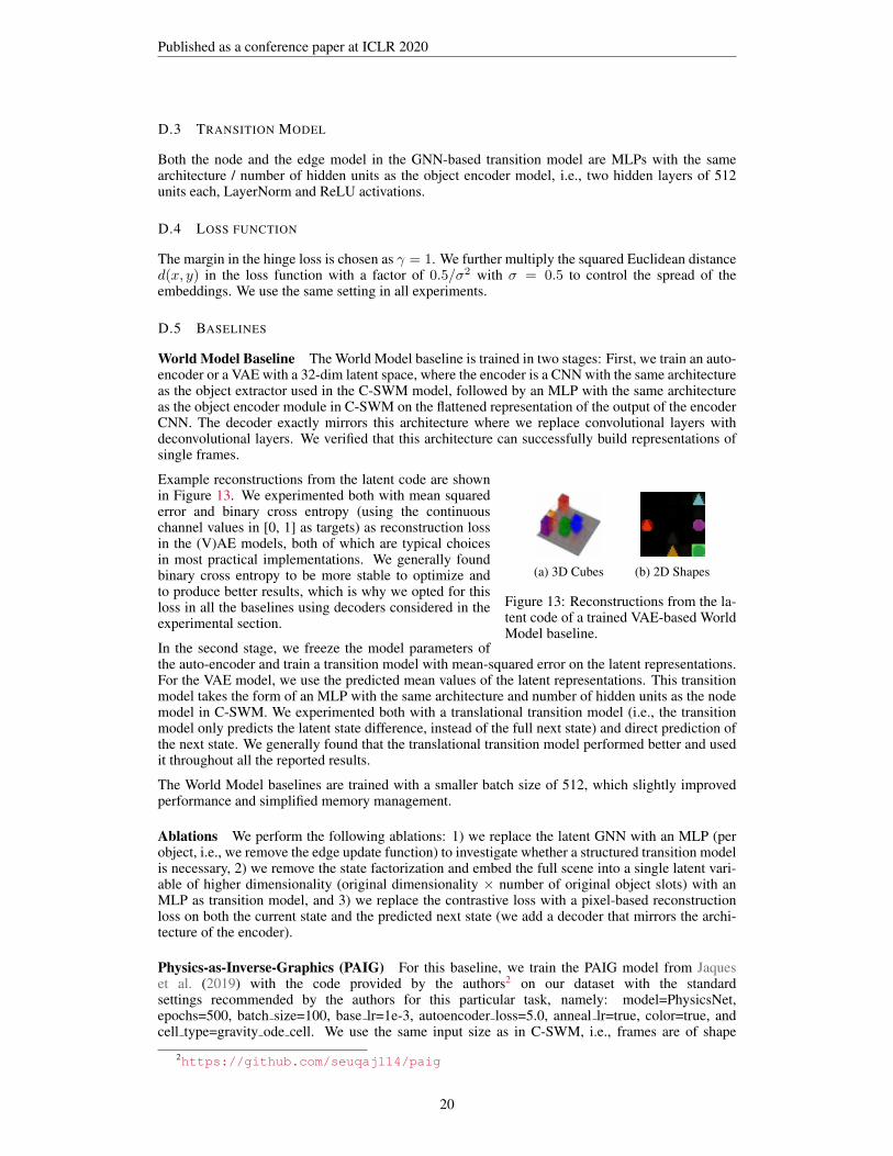
Figure 13: Reconstructions from the la-tent code of a trained VAE-based WorldModel baseline.

Example reconstructions from the latent code are shownin Figure 13. We experimented both with mean squarederror and binary cross entropy (using the continuouschannel values in [0, 1] as targets) as reconstruction lossin the (V)AE models, both of which are typical choicesin most practical implementations. We generally foundbinary cross entropy to be more stable to optimize andto produce better results, which is why we opted for thisloss in all the baselines using decoders considered in theexperimental section.

In the second stage, we freeze the model parameters ofthe auto-encoder and train a transition model with mean-squared error on the latent representations.For the VAE model, we use the predicted mean values of the latent representations. This transitionmodel takes the form of an MLP with the same architecture and number of hidden units as the nodemodel in C-SWM. We experimented both with a translational transition model (i.e., the transitionmodel only predicts the latent state difference, instead of the full next state) and direct prediction ofthe next state. We generally found that the translational transition model performed better and usedit throughout all the reported results.

The World Model baselines are trained with a smaller batch size of 512, which slightly improvedperformance and simplified memory management.

Ablations We perform the following ablations: 1) we replace the latent GNN with an MLP (perobject, i.e., we remove the edge update function) to investigate whether a structured transition modelis necessary, 2) we remove the state factorization and embed the full scene into a single latent vari-able of higher dimensionality (original dimensionality × number of original object slots) with anMLP as transition model, and 3) we replace the contrastive loss with a pixel-based reconstructionloss on both the current state and the predicted next state (we add a decoder that mirrors the archi-tecture of the encoder).

Physics-as-Inverse-Graphics (PAIG) For this baseline, we train the PAIG model from Jaqueset al. (2019) with the code provided by the authors2 on our dataset with the standardsettings recommended by the authors for this particular task, namely: model=PhysicsNet,epochs=500, batch size=100, base lr=1e-3, autoencoder loss=5.0, anneal lr=true, color=true, andcell type=gravity ode cell. We use the same input size as in C-SWM, i.e., frames are of shape

2https://github.com/seuqaj114/paig

20

https://github.com/seuqaj114/paig


50 × 50 × 3. We further set input steps=2, pred steps=10 and extrap steps=0 to match our settingof predicting for a total of 10 frames while conditioning on a pair of 2 initial frames to obtain ini-tial position and velocity information. We train this model with four different random seeds. Forevaluation, we extract learned position representations for all frames of the test set and further runthe latent physics prediction module (conditioned on the first two initial frames) to obtain modelpredictions. We further augment position representations with velocity information by taking thedifference between two consecutive position representations and concatenating this representationwith the 2-dim position representation, which we found to slightly improve results. In total, weobtain a 12-dim (4-dim × 3 objects) representation for each time step, i.e., the same as C-SWM.From this, we obtain ranking metrics. We found that one of the training runs (seed=2) collapsed alllatent representations to a single point. We exclude this run in the results reported in Table 1, i.e.,we report average and standard error over the three other runs only.

21

contrastive learning of structured world models

Documents