contribution to flight guidance in high density traffic
TRANSCRIPT

HAL Id: tel-01833564https://tel.archives-ouvertes.fr/tel-01833564v2
Submitted on 15 May 2019
HAL is a multi-disciplinary open accessarchive for the deposit and dissemination of sci-entific research documents, whether they are pub-lished or not. The documents may come fromteaching and research institutions in France orabroad, or from public or private research centers.
L’archive ouverte pluridisciplinaire HAL, estdestinée au dépôt et à la diffusion de documentsscientifiques de niveau recherche, publiés ou non,émanant des établissements d’enseignement et derecherche français ou étrangers, des laboratoirespublics ou privés.
Contribution to flight guidance in high density trafficHector Escamilla Nuñez
To cite this version:Hector Escamilla Nuñez. Contribution to flight guidance in high density traffic. Signal and ImageProcessing. Université Paul Sabatier - Toulouse III, 2018. English. NNT : 2018TOU30074. tel-01833564v2

THESETHESEEn vue de l’obtention du
DOCTORAT DE L’UNIVERSITE DE TOULOUSE
Delivre par : l’Universite Toulouse 3 Paul Sabatier (UT3 Paul Sabatier)
Presentee et soutenue le 19/06/2018 par :
Hector ESCAMILLA NUNEZ
Contribution au guidage des avions en trafic a haute densite
JURYDavid ZAMMIT MANGION Universite de Malte RapporteurJose Raul CARREIRAAZINHEIRA
Universite de Lisbonne Rapporteur
Boutaib DAHHOU Universite Paul Sabatier President du JuryFatiha NEJJARI Universite Polytechnique de
CatalogneExaminateur
Antoine DROUIN ENAC ExaminateurFelix MORA CAMINO ENAC Examinateur
Ecole doctorale et specialite :MITT : Signal, Image, Acoustique et Optimisation
Unite de Recherche :Ecole Nationale de l’Aviation Civile (ENAC), Laboratoire de Mathematiques Appliquees, In-formatique, et Automatique pour l’Aerien (MAIAA).
Directeur(s) de These :Felix MORA CAMINO et Antoine DROUIN
Rapporteurs :David ZAMMIT MANGION et Jose Raul CARREIRA AZINHEIRA


i
Declaration of AuthorshipI, Héctor ESCAMILLA NÚÑEZ, declare that this thesis titled, "Contribution toFlight Guidance in High Density Traffic" and the work presented in it are my own. Iconfirm that:
• This work was done wholly or mainly while in candidature for a research de-gree at this University.
• Where I have consulted the published work of others, this is always clearlyattributed.
• I have acknowledged all main sources of help.
Signed:
Date:


iii
“It matters not how strait the gate,How charged with punishments the scroll,I am the master of my fate,I am the captain of my soul.”
William Ernest Henley


v
Abstract
This work is developed with the perspective of SESAR and Next-Gen projects, wherenew applications of Air Traffic Management (ATM) such as the Full 4D Managementconcept, are centered on Trajectory-Based Operations (TBO), deeply related with theextension of the flexibility in separation between aircraft, and hence, with the aug-mentation of air traffic capacity.Therefore, since a shift from fixed routes and Air Traffic Control (ATC) clearances toflexible trajectories is imminent, while relying on higher levels of onboard automa-tion, the thesis hinges around topics that should enable or ease the transition fromcurrent systems to systems compliant with the new expectancies of Trajectory-BasedOperations.The main axes of the manuscript can be summarized in three topics: 4D trajectorygeneration, 4D guidance, and mass estimation for trajectory optimization.Regarding the trajectory generation, the need of airspace users to plan their pre-ferred route from an entry to an exit point of the airspace without being constrainedby the existent configurations is considered. Thus, a particular solution for 4Dsmooth path generation from preexisting control points is explored.The method is based on Bezier curves, and is able to control the Euclidian distancebetween the given control points and the proposed trajectory. This is done by re-shaping the path to remain within load factor limits, taking into account a tradeoffbetween path curvature and aircraft intended speed, representing a milestone in theroad towards Trajectory-Based Operations.It is considered that accurate 4D guidance will improve safety by decreasing theoccurrence of near mid-air collisions for planned conflict free 4D trajectories. Inconsequence, two autopilots and two guidance approaches are developed with theobjective of diminishing the workload for air traffic controllers associated to a singleflight. The backstepping and feedback linearization techniques are used for attitudecontrol, while direct and indirect nonlinear inversion are adopted for guidance.Furthermore, the impact of inaccurate mass knowledge in trajectory guidance, withconsequences in optimization, fuel consumption, and aircraft performance, has ledto the implementation of an on-board aircraft mass estimation. The created approachis based on least squares, providing an initial mass estimation, and online computa-tions of the current mass, both with enough accuracy to meet the objectives relatedto TBO.The methods proposed in this thesis are tested in a six degrees of freedom Matlabmodel with its parameters chosen similar to an aircraft type B737-200 or A320-200.The simulation is based on a full nonlinear modelling of transport aircraft dynamicsunder wind disturbances. Trained neural networks are used to obtain the aerody-namic coefficients corresponding the aircraft forces and moments.
Keywords: Trajectory Generation, Automatic control, Trajectory Tracking, Mass Esti-mation, Transport Aircraft Simulation


vii
Résumé
Ce travail est développé dans le contexte des projets SESAR et Next-Gen, où de nou-velles applications de la gestion du trafic aérien (ATM) comme le concept de gestiond’opérations en 4D, se sont focalisées sur les opérations basées sur la trajectoire (TBO- Trajectory Based Operations). Ces opérations sont en relation avec l’extension dela flexibilité de la séparation entre avions, et par conséquence, avec l’augmentationde la capacité du trafic aérien.En sachant qu’une évolution des routes fixes et autorisations émises par le contrôledu trafic aérien (ATC - Air Traffic Control) vers des trajectoires flexibles est immi-nente, en s’appuyant en même temps aux niveaux les plus élevés de l’automatiqueembarquée, ce travail de recherche s’intéresse aux sujets qui aideront à la transitiondes systèmes actuels vers les systèmes compatibles avec les nouveaux besoins desTBO.Les principaux axes de recherche de ce manuscrit s’articulent en trois points: Lagénération de trajectoires en 4D, le guidage en 4D, et l’estimation de la masse d’unavion pour l’optimisation des trajectoires.Concernant la génération des trajectoires, le besoin des utilisateurs d’espaces aériensde planifier leurs routes préférées à partir d’un point d’entrée dans l’espace aériensans être limités par les configurations existantes est considéré. Une solution parti-culière pour la génération de trajectoires lisses en 4D à partir de points de contrôleprédéfinis est alors explorée.La méthode proposée s’appuie sur les courbes de Bézier, et elle permet de contrôlerla distance euclidienne entre le point de contrôle donné et la trajectoire proposée.Ceci est fait en modifiant la trajectoire de telle façon qu’elle reste à l’intérieur deslimites des facteurs de charge, en considérant un compromis entre la courbure dela trajectoire et la vitesse voulue de l’avion, ce qui représente une étape importantedans le chemin vers les TBO.Le guidage précis en 4D améliorera la sûreté en diminuant l’occur- rence de quasi-collisions aériennes pour des trajectoires en 4D planifiées en avance. En conséquence,deux autopilotes et deux méthodes de guidage sont développées avec l’objectif deréduire la charge de travail des contrôleurs du trafic aérien associée à un vol. Lestechniques de backstepping et feedback linearization sont utilisées pour le pilotage,alors que l’inversion non linéaire directe et indirecte sont adoptées pour le guidage.De plus, l’impact de la connaissance inexacte de la masse de l’avion dans le suivi detrajectoires, ses conséquences dans l’optimisation, la consommation de carburant,et la performance de l’avion, a conduit à l’implémentation d’une estimation embar-quée de la masse de l’avion. L’approche créée est basée sur les moindres carrées, enfournissant des estimations de la masse initiale et la masse courante, toutes les deuxavec une précision suffisante pour atteindre les objectifs liées aux TBO.Les méthodes proposées dans cette thèse sont examinées en utilisant un modèle àsix degrés de liberté, dont les paramètres approchent un appareil du type B737-200ou A320-200. La simulation est basée sur une modélisation complète et non linéairede la dynamique des avions de transport incluant des perturbations liées au vent.Des réseaux de neurones sont utilisés pour obtenir les différents coefficients aérody-namiques correspondant aux forces et moments de l’avion.


ix
AcknowledgementsI would like to thank first to my parents, for their limitless love and support through-out my life. Secondly, I give my gratitude to my brother and my friends, for theirlove and sincere advice full of rawness and truth. They are all pillars of my life.To E., for encouraging me in every possible way, and for being an outstanding per-son since the day we met.
To my thesis supervisors F. Mora and A. Drouin, for accepting me in their researchenvironment and show me the different facets and commitments of a researcher.To CONACYT, for its support program to Ph.D. students, knowing that without it,this professional and personal growth would have been impossible.


xi
Contents
Declaration of Authorship i
Abstract v
Résumé vii
Acknowledgements ix
List of Abbreviations xxi
List of Constants xxiii
List of Symbols xxv
1 General Introduction 1
2 General view of Air Traffic Organization 52.1 Current Organization of Air Traffic . . . . . . . . . . . . . . . . . . . . . 6
2.1.1 Air Traffic Management (ATM) . . . . . . . . . . . . . . . . . . . 72.1.1.1 Air Traffic Services (ATS) . . . . . . . . . . . . . . . . . 72.1.1.2 Air Traffic Flow and Capacity Management (ATFCM) 122.1.1.3 Air Space Management (ASM) . . . . . . . . . . . . . . 14
2.1.2 Aeronautical Meteorology . . . . . . . . . . . . . . . . . . . . . . 172.2 Modern Air Traffic Organization . . . . . . . . . . . . . . . . . . . . . . 20
2.2.1 Freeflight . . . . . . . . . . . . . . . . . . . . . . . . . . . . . . . 242.2.2 SESAR and NextGen . . . . . . . . . . . . . . . . . . . . . . . . . 27
2.2.2.1 Implementation of TBO . . . . . . . . . . . . . . . . . . 292.3 Conclusion . . . . . . . . . . . . . . . . . . . . . . . . . . . . . . . . . . . 31
3 Flight Dynamics of Transport Aircraft under Wind Disturbances 333.1 Reference Frames . . . . . . . . . . . . . . . . . . . . . . . . . . . . . . . 34
3.1.1 Adopted frames . . . . . . . . . . . . . . . . . . . . . . . . . . . . 343.1.1.1 Inertial Frame . . . . . . . . . . . . . . . . . . . . . . . 343.1.1.2 Earth-fixed Reference Frame . . . . . . . . . . . . . . . 343.1.1.3 Body Reference Frame . . . . . . . . . . . . . . . . . . 343.1.1.4 Stability Reference Frame . . . . . . . . . . . . . . . . . 343.1.1.5 Wind Reference Frame . . . . . . . . . . . . . . . . . . 34
3.1.2 Rotation Matrices between frames . . . . . . . . . . . . . . . . . 363.2 Equations of motion . . . . . . . . . . . . . . . . . . . . . . . . . . . . . 38
3.2.1 Guidance Dynamics . . . . . . . . . . . . . . . . . . . . . . . . . 383.2.2 Attitude Dynamics . . . . . . . . . . . . . . . . . . . . . . . . . . 393.2.3 Dynamics in the wind frame . . . . . . . . . . . . . . . . . . . . 423.2.4 Actuator Dynamics . . . . . . . . . . . . . . . . . . . . . . . . . . 43
3.3 Reduced equations of motion . . . . . . . . . . . . . . . . . . . . . . . . 45

xii
3.3.1 Longitudinal Motion . . . . . . . . . . . . . . . . . . . . . . . . . 453.3.1.1 Level Flight . . . . . . . . . . . . . . . . . . . . . . . . . 47
3.3.2 Lateral-directional Motion . . . . . . . . . . . . . . . . . . . . . . 473.3.2.1 Steady turn . . . . . . . . . . . . . . . . . . . . . . . . . 48
3.4 Dimensionless Aerodynamic Coefficients . . . . . . . . . . . . . . . . . 493.5 Load factor . . . . . . . . . . . . . . . . . . . . . . . . . . . . . . . . . . . 513.6 Compilation of equations . . . . . . . . . . . . . . . . . . . . . . . . . . 54
3.6.1 Complete Aircraft Dynamics . . . . . . . . . . . . . . . . . . . . 543.6.1.1 Guidance equations . . . . . . . . . . . . . . . . . . . . 543.6.1.2 Attitude equations . . . . . . . . . . . . . . . . . . . . . 543.6.1.3 Actuator equations . . . . . . . . . . . . . . . . . . . . 54
3.6.2 Reduced Aircraft Dynamics . . . . . . . . . . . . . . . . . . . . . 553.6.2.1 Longitudinal motion . . . . . . . . . . . . . . . . . . . 553.6.2.2 Lateral motion . . . . . . . . . . . . . . . . . . . . . . . 55
3.6.3 Load Factor equations . . . . . . . . . . . . . . . . . . . . . . . . 553.7 Conclusion . . . . . . . . . . . . . . . . . . . . . . . . . . . . . . . . . . . 56
4 6DOF Transport Aircraft Simulation using MATLAB 574.1 Aerodynamic Coefficients using Neural Networks . . . . . . . . . . . . 58
4.1.1 Introduction to Machine Learning . . . . . . . . . . . . . . . . . 584.1.1.1 Polynomial Curve fitting . . . . . . . . . . . . . . . . . 584.1.1.2 Bayesian Approach . . . . . . . . . . . . . . . . . . . . 594.1.1.3 Bayesian curve fitting . . . . . . . . . . . . . . . . . . . 634.1.1.4 Model Selection . . . . . . . . . . . . . . . . . . . . . . 644.1.1.5 Linear Models for Regression . . . . . . . . . . . . . . 64
4.1.2 Neural Networks Model . . . . . . . . . . . . . . . . . . . . . . . 654.1.3 Aerodynamic Coefficients . . . . . . . . . . . . . . . . . . . . . . 67
4.1.3.1 Lift and Drag Coefficients . . . . . . . . . . . . . . . . 694.1.3.2 Sideforce Coefficient . . . . . . . . . . . . . . . . . . . . 694.1.3.3 Rolling moment . . . . . . . . . . . . . . . . . . . . . . 714.1.3.4 Yawing Coefficient . . . . . . . . . . . . . . . . . . . . . 754.1.3.5 Pitching Coefficient . . . . . . . . . . . . . . . . . . . . 77
4.2 Simulation of Aircraft Dynamics in Open Loop . . . . . . . . . . . . . . 804.3 Data Visualization through FlightGear flight simulator . . . . . . . . . 854.4 Conclusions . . . . . . . . . . . . . . . . . . . . . . . . . . . . . . . . . . 86
5 4D Trajectory Generation for Transport Aircraft using Bezier curves 875.1 Introduction . . . . . . . . . . . . . . . . . . . . . . . . . . . . . . . . . . 885.2 Bezier Curves Definition . . . . . . . . . . . . . . . . . . . . . . . . . . . 92
5.2.1 Continuity and Curvature of a Curve . . . . . . . . . . . . . . . 935.3 Trajectory Generation . . . . . . . . . . . . . . . . . . . . . . . . . . . . . 96
5.3.1 G2 Continuity Path Generation . . . . . . . . . . . . . . . . . . . 965.3.2 Time-Parametrization of the Path . . . . . . . . . . . . . . . . . . 98
5.4 Reshaping of the Trajectory . . . . . . . . . . . . . . . . . . . . . . . . . 1015.5 Load Factor and Curvature of the Trajectory . . . . . . . . . . . . . . . . 1055.6 Generation of a full Flight Profile . . . . . . . . . . . . . . . . . . . . . . 110
5.6.1 Multiplicity of trajectories . . . . . . . . . . . . . . . . . . . . . . 1135.7 Conclusion . . . . . . . . . . . . . . . . . . . . . . . . . . . . . . . . . . . 114

xiii
6 Aircraft Mass Estimation 1156.1 Introduction . . . . . . . . . . . . . . . . . . . . . . . . . . . . . . . . . . 116
6.1.1 Base of Aircraft Data (BADA) . . . . . . . . . . . . . . . . . . . . 1196.1.1.1 BADA Fuel Consumption Model . . . . . . . . . . . . 120
6.1.2 Fuel Consumption Model of the ICAO Engine Emission Data-bank . . . . . . . . . . . . . . . . . . . . . . . . . . . . . . . . . . 120
6.2 Mass Estimations based on the longitudinal equations of motion . . . . 1236.3 Mass Estimation based on Least Squares . . . . . . . . . . . . . . . . . . 1286.4 Conclusions . . . . . . . . . . . . . . . . . . . . . . . . . . . . . . . . . . 132
7 Introduction to Control Theory 1337.1 Linear Systems Theory . . . . . . . . . . . . . . . . . . . . . . . . . . . . 134
7.1.1 First and Second Order Systems . . . . . . . . . . . . . . . . . . 1347.1.1.1 First Order Systems . . . . . . . . . . . . . . . . . . . . 1347.1.1.2 State-Space Representation and General Solution of
Linear Time Invariant Systems . . . . . . . . . . . . . . 1377.1.1.3 Second Order Systems . . . . . . . . . . . . . . . . . . 138
7.1.2 Stability of Linear Systems . . . . . . . . . . . . . . . . . . . . . 1457.1.2.1 Input-Output Stability of LTI systems . . . . . . . . . . 1457.1.2.2 Internal Stability of LTI systems . . . . . . . . . . . . . 145
7.1.3 Controllability and Observability of Linear Systems . . . . . . . 1467.1.4 Control Approaches of Linear Systems . . . . . . . . . . . . . . 147
7.1.4.1 State-Feedback . . . . . . . . . . . . . . . . . . . . . . . 1477.1.4.2 PID control . . . . . . . . . . . . . . . . . . . . . . . . . 148
7.2 Nonlinear Systems Theory . . . . . . . . . . . . . . . . . . . . . . . . . . 1497.2.1 Autonomous Systems . . . . . . . . . . . . . . . . . . . . . . . . 149
7.2.1.1 Equilibrium point . . . . . . . . . . . . . . . . . . . . . 1507.2.1.2 Stability in the sense of Lyapunov . . . . . . . . . . . . 1507.2.1.3 Asymptotic and Exponential Stability . . . . . . . . . . 1507.2.1.4 Local and Global Stability . . . . . . . . . . . . . . . . 1517.2.1.5 Lyapunov’s Linearization Method . . . . . . . . . . . . 1517.2.1.6 Lyapunov’s Direct Method . . . . . . . . . . . . . . . . 1527.2.1.7 Invariant Set Theorems . . . . . . . . . . . . . . . . . . 153
7.2.2 Non-autonomous Systems . . . . . . . . . . . . . . . . . . . . . . 1557.2.2.1 Preliminaries . . . . . . . . . . . . . . . . . . . . . . . . 1557.2.2.2 Barbalat’s Lemma . . . . . . . . . . . . . . . . . . . . . 156
7.2.3 Control Approaches for Nonlinear systems . . . . . . . . . . . . 1567.2.3.1 Feedback linearization . . . . . . . . . . . . . . . . . . 156
7.3 Modern Flight Guidance Systems . . . . . . . . . . . . . . . . . . . . . . 1607.4 Conclusion . . . . . . . . . . . . . . . . . . . . . . . . . . . . . . . . . . . 163
8 4D Guidance Control for Transport Aircraft 1658.1 Attitude Control . . . . . . . . . . . . . . . . . . . . . . . . . . . . . . . . 166
8.1.1 Backstepping . . . . . . . . . . . . . . . . . . . . . . . . . . . . . 1668.1.1.1 Numerical Simulation . . . . . . . . . . . . . . . . . . . 170
8.1.2 Non Linear Inversion . . . . . . . . . . . . . . . . . . . . . . . . 1728.1.2.1 Numerical Simulation . . . . . . . . . . . . . . . . . . . 175
8.2 Guidance Control . . . . . . . . . . . . . . . . . . . . . . . . . . . . . . . 1808.2.1 Non Linear Inversion . . . . . . . . . . . . . . . . . . . . . . . . 180
8.2.1.1 Stability of direct NLI Guidance Control using Lya-punov theory . . . . . . . . . . . . . . . . . . . . . . . . 183

xiv
8.2.1.2 Numerical Simulation . . . . . . . . . . . . . . . . . . . 1848.2.1.3 Sensitivity analysis with respect to wind disturbances
for the direct NLI approach . . . . . . . . . . . . . . . . 1878.2.2 Total Energy . . . . . . . . . . . . . . . . . . . . . . . . . . . . . . 1898.2.3 Guidance Control based on indirect NLI . . . . . . . . . . . . . 190
8.2.3.1 Numerical Simulation . . . . . . . . . . . . . . . . . . . 1928.3 Conclusion . . . . . . . . . . . . . . . . . . . . . . . . . . . . . . . . . . . 195
9 Conclusions and Perspectives 1979.1 General Conclusions . . . . . . . . . . . . . . . . . . . . . . . . . . . . . 197
9.1.1 Trajectory Generation . . . . . . . . . . . . . . . . . . . . . . . . 1979.1.1.1 Numerical Simulation of an Aircraft . . . . . . . . . . 198
9.1.2 Flight Control Systems . . . . . . . . . . . . . . . . . . . . . . . . 1999.1.2.1 Aircraft Mass Estimation . . . . . . . . . . . . . . . . . 200
9.2 Future Work . . . . . . . . . . . . . . . . . . . . . . . . . . . . . . . . . . 2019.2.1 Trajectory Generation . . . . . . . . . . . . . . . . . . . . . . . . 201
9.2.1.1 Numerical Simulation of an Aircraft . . . . . . . . . . 2019.2.2 Flight Control Systems . . . . . . . . . . . . . . . . . . . . . . . . 201
9.2.2.1 Aircraft Mass Estimation . . . . . . . . . . . . . . . . . 202
A Coordinate Transformations 203A.1 Transformation of a Vector . . . . . . . . . . . . . . . . . . . . . . . . . . 203A.2 The Rotation Matrix . . . . . . . . . . . . . . . . . . . . . . . . . . . . . . 204A.3 Transformation of the Derivative of a vector . . . . . . . . . . . . . . . . 205
B Gaussian Distribution 207B.1 Mathematical Representation . . . . . . . . . . . . . . . . . . . . . . . . 207
B.1.1 Univariate Gaussian Distribution . . . . . . . . . . . . . . . . . . 207B.1.2 Multivariate Gaussian Distribution . . . . . . . . . . . . . . . . 207
B.2 Regression applied to a Gaussian distribution using the MaximumLikelihood approach . . . . . . . . . . . . . . . . . . . . . . . . . . . . . 209
C Neural Networks Performance 211
List of Publications 215
Bibliography 217

xv
List of Figures
2.1 Example of an TCAS time/altitude Volume of Protection (Wikipedia,2017). . . . . . . . . . . . . . . . . . . . . . . . . . . . . . . . . . . . . . . 10
2.2 Tower Control Unit (KLM, 2017). . . . . . . . . . . . . . . . . . . . . . . 122.3 Approach/Terminal Control Unit (StackExchange, 2017a). . . . . . . . 122.4 Handling of Air Traffic (StackExchange, 2017b). . . . . . . . . . . . . . 132.5 Classification of Airspace (FAA, 2017). . . . . . . . . . . . . . . . . . . . 142.6 Aeronautical charts (SkyVector, 2017). . . . . . . . . . . . . . . . . . . . 172.7 Common MET information (SkyVector, 2017). . . . . . . . . . . . . . . . 192.8 Comparison between Conventional, RNAV, and RNP routes. . . . . . . 212.9 Error definition in RNP. . . . . . . . . . . . . . . . . . . . . . . . . . . . 212.10 Navigation specifications for different flight phases. . . . . . . . . . . . 222.11 Free Flight implementation (Eurocontrol, 2017i). . . . . . . . . . . . . . 262.12 Concept of CDO (Eurocontrol October 2011). . . . . . . . . . . . . . . . . 30
3.1 Earth frame and Body frame. . . . . . . . . . . . . . . . . . . . . . . . . 353.2 Wind frame and Stability frame. AoA and Sideslip angle in the posi-
tive sense. . . . . . . . . . . . . . . . . . . . . . . . . . . . . . . . . . . . 353.3 Forces acting on an aircraft. . . . . . . . . . . . . . . . . . . . . . . . . . 383.4 Positive sense of velocities and aerodynamic forces and moments. . . . 413.5 Flight Path Angle. . . . . . . . . . . . . . . . . . . . . . . . . . . . . . . . 453.6 Steady turn forces. . . . . . . . . . . . . . . . . . . . . . . . . . . . . . . 523.7 Pitch up motion. . . . . . . . . . . . . . . . . . . . . . . . . . . . . . . . . 53
4.1 Neural Network architecture. . . . . . . . . . . . . . . . . . . . . . . . . 674.2 Aircraft drawing (Dimensions in feet). . . . . . . . . . . . . . . . . . . . 694.3 Coefficient CL. . . . . . . . . . . . . . . . . . . . . . . . . . . . . . . . . . 704.4 Coefficient CD. . . . . . . . . . . . . . . . . . . . . . . . . . . . . . . . . . 704.5 Coefficient CYβ . . . . . . . . . . . . . . . . . . . . . . . . . . . . . . . . . 714.6 Top and front view of a plane showing a positive β. The right and
left wings are in low positions and are denoted by R, L, respectively.Positive sweep angle of the wings along with a positive wing dihedralis also shown. . . . . . . . . . . . . . . . . . . . . . . . . . . . . . . . . . 71
4.7 Coefficient Clβ . . . . . . . . . . . . . . . . . . . . . . . . . . . . . . . . . 734.8 Coefficient Clp . . . . . . . . . . . . . . . . . . . . . . . . . . . . . . . . . . 734.9 Coefficient Clr . . . . . . . . . . . . . . . . . . . . . . . . . . . . . . . . . . 744.10 Coefficient Cnβ . . . . . . . . . . . . . . . . . . . . . . . . . . . . . . . . . 764.11 Coefficient Cnp . . . . . . . . . . . . . . . . . . . . . . . . . . . . . . . . . 764.12 Coefficient Cnr . . . . . . . . . . . . . . . . . . . . . . . . . . . . . . . . . 774.13 Coefficient Cmα . . . . . . . . . . . . . . . . . . . . . . . . . . . . . . . . . 784.14 Coefficient Cmq . . . . . . . . . . . . . . . . . . . . . . . . . . . . . . . . . 794.15 Block diagram of the aircraft simulation. . . . . . . . . . . . . . . . . . . 804.16 Thrust vs Airspeed graph indicating values of AoA at FL320. . . . . . . 814.17 Thrust vs Airspeed graph indicating values of AoA at FL020. . . . . . . 82

xvi
4.18 Longitudinal response of aircraft. . . . . . . . . . . . . . . . . . . . . . . 834.19 Longitudinal response of aircraft (zoom). . . . . . . . . . . . . . . . . . 834.20 Lateral response of aircraft. . . . . . . . . . . . . . . . . . . . . . . . . . 844.21 FlightGear Simulation using Matlab dynamic model. . . . . . . . . . . 85
5.1 Block diagram of the Trajectory Generation algorithm. . . . . . . . . . . 915.2 Second order Bezier curve example. . . . . . . . . . . . . . . . . . . . . 935.3 Different types of continuity in a curve. . . . . . . . . . . . . . . . . . . 955.4 G2 and G1 continuity path with auxiliary control points. . . . . . . . . 975.5 Bezier curve completed with starting and ending straight lines. . . . . 985.6 Generated path based on quintic Bezier curves. . . . . . . . . . . . . . . 995.7 Generated path showing arc lengths and joints of Bezier curves. . . . . 995.8 Curvature of the G1 and G2 continuity paths. . . . . . . . . . . . . . . . 1005.9 100m deviation reshaped path for a triplet of control points using an
auxiliary control point (Q3). . . . . . . . . . . . . . . . . . . . . . . . . . 1015.10 Curvature for a triplet of control points of the 100m deviation re-
shaped G2 path, and the G1 initial path. . . . . . . . . . . . . . . . . . . 1035.11 100m deviation reshaped path. . . . . . . . . . . . . . . . . . . . . . . . 1045.12 Curvature of reshaped path. . . . . . . . . . . . . . . . . . . . . . . . . . 1045.13 Control points of example, Arc lengths, and Times. . . . . . . . . . . . . 1065.14 Load factor at different velocities. . . . . . . . . . . . . . . . . . . . . . . 1065.15 Curvature at different velocities. . . . . . . . . . . . . . . . . . . . . . . 1075.16 Zoom to the generated trajectory close to the control point P2 with a
10m maximum deviation. . . . . . . . . . . . . . . . . . . . . . . . . . . 1075.17 Load factor and Curvature of the trajectory with a 10m maximum de-
viation. . . . . . . . . . . . . . . . . . . . . . . . . . . . . . . . . . . . . . 1085.18 Zoom to the generated trajectory close to the control point P2 forcing
a maximum load factor compared with Reshaping algorithm. . . . . . 1095.19 Load factor and Curvature of the trajectory close to the control point
P2 with a maximum load factor. . . . . . . . . . . . . . . . . . . . . . . . 1095.20 Vertical profile from flight AF7527 (Flightradar24, 2017). . . . . . . . . 1105.21 Lateral profile from flight AF7527. . . . . . . . . . . . . . . . . . . . . . 1105.22 Reproduction of the lateral/vertical profile of the flight AF7527. . . . . 1115.23 Multiplicity of the flight profile. . . . . . . . . . . . . . . . . . . . . . . . 113
6.1 Different weights of an aircraft (StackExchange, 2017c). . . . . . . . . . 1166.2 Performance Table file of an A320 (Eurocontrol, 2017d). . . . . . . . . . 1216.3 Mass estimation scheme. . . . . . . . . . . . . . . . . . . . . . . . . . . . 1236.4 Altitude and Rate of Climb for mass inference. . . . . . . . . . . . . . . 1256.5 Variables used to infer aircraft mass and Thrust profile. . . . . . . . . . 1256.6 Fuel consumption and Thrust profile inference. . . . . . . . . . . . . . . 1266.7 Mass inference at different sampling times. . . . . . . . . . . . . . . . . 1276.8 Initial mass estimation. . . . . . . . . . . . . . . . . . . . . . . . . . . . . 1296.9 Initial mass estimation and initial mass inference errors at different
sampling times. . . . . . . . . . . . . . . . . . . . . . . . . . . . . . . . . 1306.10 Mass estimation using initial mass estimations. . . . . . . . . . . . . . . 1306.11 Mass estimation and mass inference errors at different sampling times. 131
7.1 First order linear systems zero-input response (MIT, 2017). . . . . . . . 1357.2 Step response of 1st order systems (MIT, 2017). . . . . . . . . . . . . . . 1357.3 Impulse response of 1st order systems (MIT, 2017). . . . . . . . . . . . . 136

xvii
7.4 Unit ramp response of 1st order systems (MIT, 2017). . . . . . . . . . . 1367.5 Overdamped and critically damped zero-input response of 2nd order
systems with y(0) = 1 and y(0) = 0 (MIT, 2017). . . . . . . . . . . . . . 1407.6 Underdamped and critically damped zero-input response of 2nd or-
der systems with y(0) = 1 and y(0) = 0 (MIT, 2017). . . . . . . . . . . . 1417.7 Poles of 2nd order systems at different damping factors (MIT, 2017). . 1427.8 Step response of 2nd order systems with y(0) = 0 and y(0) = 0 (MIT,
2017). . . . . . . . . . . . . . . . . . . . . . . . . . . . . . . . . . . . . . . 1437.9 Impulse response of 2nd order systems with y(0) = 0 and y(0) = 0
(MIT, 2017). . . . . . . . . . . . . . . . . . . . . . . . . . . . . . . . . . . 1437.10 Convergence to the invariant set M. . . . . . . . . . . . . . . . . . . . . 1547.11 Classical structure of Flight Control Systems (Mora-Camino, 2017). . . 160
8.1 Block diagram of the backstepping controller. . . . . . . . . . . . . . . . 1698.2 φ, α and β response. . . . . . . . . . . . . . . . . . . . . . . . . . . . . . 1708.3 Attitude control behaviour. . . . . . . . . . . . . . . . . . . . . . . . . . 1708.4 Attitude control behaviour at different frequencies. . . . . . . . . . . . 1718.5 Attitude control behaviour at different frequencies. . . . . . . . . . . . 1718.6 Block diagram of the NLI controller. . . . . . . . . . . . . . . . . . . . . 1748.7 Attitude control behaviour. . . . . . . . . . . . . . . . . . . . . . . . . . 1758.8 Control effort. . . . . . . . . . . . . . . . . . . . . . . . . . . . . . . . . . 1758.9 Attitude response to disturbances. . . . . . . . . . . . . . . . . . . . . . 1768.10 Pitch rate response. . . . . . . . . . . . . . . . . . . . . . . . . . . . . . . 1778.11 Roll rate response. . . . . . . . . . . . . . . . . . . . . . . . . . . . . . . . 1778.12 Slip/Skid Indicator for turn coordination. The ball to the right indi-
cates slip and to the left indicates skid. Only gravity forces affect theball position (CFI, 2017). . . . . . . . . . . . . . . . . . . . . . . . . . . . 178
8.13 Yaw rate step response . . . . . . . . . . . . . . . . . . . . . . . . . . . . 1798.14 Block diagram of the direct NLI controller. . . . . . . . . . . . . . . . . 1838.15 Guidance control test . . . . . . . . . . . . . . . . . . . . . . . . . . . . . 1858.16 Guidance response to a 100m step with constant thrust. . . . . . . . . . 1858.17 Longitudinal response to a 100m step with a variable thrust. . . . . . . 1868.18 Longitudinal response to a 300m step with constant and variable thrust.1868.19 Position response to disturbances. . . . . . . . . . . . . . . . . . . . . . 1878.20 Wind knowledge effect on position errors. . . . . . . . . . . . . . . . . . 1888.21 Change in ψ required to follow the reference trajectory . . . . . . . . . 1928.22 Block diagram of the indirect NLI controller. . . . . . . . . . . . . . . . 1928.23 Trajectory tracking control law simulation. . . . . . . . . . . . . . . . . 1938.24 Y desired stands for yR. Y stands for yE . Heading and roll angles are
also shown. . . . . . . . . . . . . . . . . . . . . . . . . . . . . . . . . . . 193
9.1 Panoramic view of the proposed control approaches. . . . . . . . . . . 1999.2 Dynamic protection area depending on wind direction. . . . . . . . . . 201
A.1 Basic rotation about xa1. . . . . . . . . . . . . . . . . . . . . . . . . . . . 204
C.1 Performance of the proposed CL coefficient. . . . . . . . . . . . . . . . . 211C.2 Performance of the proposed CYβ coefficient. . . . . . . . . . . . . . . . 211C.3 Performance of the proposed Clβ coefficient. . . . . . . . . . . . . . . . 212C.4 Performance of the proposed Clp coefficient. . . . . . . . . . . . . . . . 212C.5 Performance of the proposed Clr coefficient. . . . . . . . . . . . . . . . 212C.6 Performance of the proposed Cmα coefficient. . . . . . . . . . . . . . . . 213

xviii
C.7 Performance of the proposed Cmq coefficient. . . . . . . . . . . . . . . . 213C.8 Performance of the proposed Cnβ coefficient. . . . . . . . . . . . . . . . 213C.9 Performance of the proposed Cnp coefficient. . . . . . . . . . . . . . . . 214C.10 Performance of the proposed Cnr coefficient. . . . . . . . . . . . . . . . 214

xix
List of Tables
2.1 Airspace Classification . . . . . . . . . . . . . . . . . . . . . . . . . . . . 15
5.1 Control Points. . . . . . . . . . . . . . . . . . . . . . . . . . . . . . . . . . 995.2 Times and Arc lengths. . . . . . . . . . . . . . . . . . . . . . . . . . . . . 1005.3 Distance of curve from control points. . . . . . . . . . . . . . . . . . . . 1035.4 Control points for an aircraft changing airways. . . . . . . . . . . . . . 1055.5 Arc lengths and times at different velocities . . . . . . . . . . . . . . . . 1065.6 Auxiliary control points to force a high load factor . . . . . . . . . . . . 1085.7 Flight Profile of AF7527. . . . . . . . . . . . . . . . . . . . . . . . . . . . 112
6.1 Fuel flow coefficients . . . . . . . . . . . . . . . . . . . . . . . . . . . . . 1206.2 Fuel Consumption data. . . . . . . . . . . . . . . . . . . . . . . . . . . . 1226.3 Maximum Thrust provided by engines used in A320-200/B737-200 . . 1226.4 Percentage of Thrust used in different flight phases . . . . . . . . . . . 122
7.1 Characteristic responses of y + 2ζωny + ω2ny = f(t) (MIT, 2017). . . . . 144
7.2 Gain Computation for a PID controller (Ziegler-Nichols). . . . . . . . . 148
8.1 Error depending on Wind knowledge . . . . . . . . . . . . . . . . . . . 1888.2 Controllers summary . . . . . . . . . . . . . . . . . . . . . . . . . . . . . 196


xxi
List of Abbreviations
ABAS Aircraft Based Augmentation Systema.c. Aerodynamic CenterACAS Airborne Collision Avoidance SystemsACC Area Control CentreADS-B Automatic Dependent Surveillance – BroadcastAGL Above Ground LevelAIS/AIM Aeronautical Information Services/ManagementANSP Air Navigation Service ProviderAoA Angle of AttackARTCC Air Route Traffic Control CenterASAS Airborne Separation Assistance SystemASM Air Space ManagementATC Air Traffic ControlATFCM Air Traffic Flow and Capacity ManagementATM Air Traffic ManagementATS Air Traffic ServicesATSAW Airborne Traffic Situational AWarenessBADA Base of Aircraft DAtaCANSO Civil Air Navigation Services OrganisationCAS Calibrated Air SpeedCDM Collaborative Decision MakingCDO/CCO Continuous Descent/Climb Operationsc.g. Center of GravityCNS Communications, Navigation and Surveillance SystemsDCAC Direction Générale de l’Aviation CivileDOF Degrees Of FreedomDME Distance Measuring EquipmentDSNA Direction des Services de la Navigation AérienneEOW Empty Operating WeightFAB Functional Airspace BlockFANS Future Air Navigation SystemsFCU Flight Control UnitFDR Flight Data RecorderFGS Flight Guidance SystemsFIR Flight Information RegionFIS/-B Flight Information Service / - BroadcastFL Flight LevelFMS Flight Management SystemFPA Flight Path AngleFRA Free Route AirspaceGBAS Ground Based Augmentation SystemsGNSS Global Navigation Satellite SystemsGTOW Gross Take-Off Weight

xxii
IAS Indicated Air SpeedICAO International Civil Aviation OrganizationIFR Instrument Flight RulesILS Instrument Landing SystemINS Inertial Navigation SystemIRU Inertial Reference UnitMCDU Multipurpose Control Display UnitMET Aeronautical METeorology Service for Air NavigationMLS Microwave Landing SystemNLI Non Linear InversionNDB Non Directional BeaconNN Neural NetowrkPBN Performance Based NavigationPFD Primary Flight DisplayRBT Reference Business TrajectoryRNP Required Navigation PerformanceRVR Runway Visual RangeSAR Search And RescueSBAS Satellite - Based Augmentation SystemsSSR Secondary Surveillance RadarSVFR Special Visual Flight RulesTAS True Air SpeedTCAS Traffic Collision Avoidance SystemTIS-B Traffic Information Service - BroadcastTBO Trajectory Based OperationsTMA Terminal Manoeuvring AreaTOW Take-Off WeightTRACON Terminal Radar Approach CONtrolVFR Visual Flight RulesVHF Very High FrequencyVOR Very High Frequency Omnidirectional RangeVoP Volume of Protectionw.r.t. with respect toZFW Zero Fuel Weight

xxiii
List of Constants
Aircraft c.g. position Xcg = 15.3 mAircraft c.g. position Ycg = 0 mAircraft c.g. position Zcg = −1.016 mControl surfaces time-constants ξail,ele,rud = .05 sInertia matrix component A = 1, 278, 369.56 kg· m2
Inertia matrix component B = 3, 781, 267.79 kg·m2
Inertia matrix component C = 4, 877, 649.98 kg·m2
Inertia matrix component E = 135, 588.17 kg·m2
Maximum speed Vmax = 0.85 MachMean chord c = 4.35 mPitching due to aircraft c.g. offset w.r.t. the a.c. coefficient Cm0 = −0.094Pitching due to elevator deflection coefficient Cmδele = −0.003 rad−1
Rolling due to ailerons deflection coefficient Clδail = −0.02 rad−1
Rolling due to ruder deflection coefficient Clδrud = 0 rad−1
Service ceiling hmax = 10, 700 mThrust time-constant ξT = 2.5 sWing area S = 123.55 m2
Wingspan b = 28.34 mYawing due to ailerons deflection coefficient Cnδail = 0.002 rad−1
Yawing due to ruder deflection coefficient Cnδrud = −0.07 rad−1


xxv
List of Symbols
CL, CD, CY Lift/Drag/Sideforce aerodynamic coefficientsCl, Cm, Cn Rolling/Pitching/Yawing aerodynamic coefficientsfE Resultant force in the earth frame acting on the aircraft NFthr, L,D, Y Thrust/Lift/Drag/Sideforce NFxa , Fya , Fza Aerodynamic Forces in the body frame Ng Gravity m/s2
hE Angular momentum in the earth frame kg ·m2/sI Inertia Matrix kg·m2
LEB Rotation matrix from the body to earth frameLBW Rotation matrix from the wind to body frameMext = [L′,M,N ]T Rolling/Pitching/Yawing moments N·mm Aircraft mass kg
ncg = [nx, ny, nz]T Load Factor in the body frame g
q Free-stream dynamic pressure kg/(m·s2)u, v, w Groundspeed in the body frame m/sVa Airspeed in the wind frame m/sVab Airspeed in the body frame m/s
VW =[VWx , VWy , VWz
]T Wind in the body frame m/sW Aircraft weight NWapp Apparent weight of the aircraft NXE , YE , ZE Aircraft position in the earth frame m
α Angle of Attack
αm AoA required to fly at minimum Thrust
β Sideslip Angle
δ = [δail, δele, δrud]T Deflection of aileron/elevator/rudder
η = [φ, θ, ψ]T Euler angles (roll, pitch, yaw)
γ Flight Path Angle
µ Thrust specific fuel consumption kg/(N·s)Ω = [p, q, r]T Angular velocities /sωd Damped natural frequency rad/sωn Undamped natural frequency rad/s
ρ Air density kg/m3
σ Standard deviationζ Damping ratio of second order systems


xxvii
A mis padres . . .A México, mi tierra natal con amor . . .


1
Chapter 1
General Introduction
Air traffic is experiencing a sustained growth since the last decades, provoking thesaturation of the main air spaces in large areas of many countries. Moreover, airtraffic is expected to increase even more in the upcoming years. In 2012, 9.5 millionflights and 0.7 billion passengers were processed, but for 2035, 14.4 million flightswith 1.4 billion passengers are expected (Eurocontrol, 2016). In general terms, twiceof today’s flight demand is expected over the next 20 years.Therefore, it is a fact that current Air Traffic Management (ATM) infrastructure willnot be able to support the growing demand unless refinements and enhancementsare addressed towards an improved ATM service.In consequence, research projects such as SESAR JU (Single European Sky ATM Re-search Joint Undertaking) and Next-Gen (Next Generation Air Transportation Sys-tem) are in charge of the development and deployment of the necessary items tobuild the world’s future air transportation system.Among all the objectives encompassed within these projects, two main items seempertinent:
1. Strategic datalink services for information sharing.
2. Negotiation between Air Traffic Control (ATC) constraints and aircraft prefer-ences in order to ensure an optimal use of airspace, while allowing aircraft tofly their preferred trajectories under the 4D guidance paradigm.
For this research work, the second point is of great interest.Current Flight Guidance Systems (FGS) for transport aircraft operate in a mode-based logic, where the Flight Management System (FMS) switches different con-trol strategies (modes) to achieve specific control objectives. These control strategiesare currently based on linear control theory, using either PID controllers, or State-Feedback linear approaches. However, since wind disturbances remain as one ofthe main causes of guidance errors, these guidance techniques need to be improved.Therefore, the first objective of this research is to develop a nonlinear control strategyincluding both guidance and piloting loops, capable of taking into account wind dis-turbances, such that an enhanced tracking performance is achieved. Furthermore,considering that the approaches used to develop these guidance strategies rely on anumerical inversion of the aircraft model, better knowledge of the aircraft parame-ters is tough to improve the numerical inversion accuracy, and therefore, lead to abetter guidance performance. In this work, the aircraft mass is considered a game-changer in terms of performance, such that a method to estimate this parameter isdeveloped.In addition to this, worldwide stakeholders are interested in flying their preferredroutes. However, current ATC structure seems too rigid to support such action, andthe unpredictability of aircraft operations eliminates the possibility of planning an

2 Chapter 1. General Introduction
intended trajectory free of conflicts. In this way, with the view of increasing trafficsafety and airspace capacity, the second objective of this manuscript is to providea trajectory generation device able to better manage air traffic flows while meetinga set of flight profile constraints, which vary in general from flight to flight. Themethod proposed, should be able to address potential conflict resolution, allow air-craft to fly closer, and display the same functionalities of current flight planing de-vices.Since the numerical feasibility of the presented approaches needs to be analyzed, thenumerical simulation of a transport aircraft is needed. Thus, an important action ofthis thesis dissertation arises.Stated this, the principal objectives of the thesis can be summarized in two items(O.1 and O.2), along with two needed actions (A.1 and A.2):
• O.1 Development of a Trajectory Generation Algorithm valid for 4D Guidance.
• O.2 Development of an Autopilot and a 4D Guidance Strategy for TransportAircraft.
A.1 Numerical Simulation of a 6DOF Transport Aircraft.
A.2 Aircraft Mass Estimation.
In order to better present the efforts and findings towards the principal objectives ofthis research, the manuscript is organized as follows:
Chapter 2 provides a panoramic vision of the current organization of Air trafficand its evolution towards the Trajectory-Based Operations paradigm, motivated bythe expected growth of air traffic in the upcoming years and its related issues. Thisis crucial to understand the context that drives the contributions tackled in this re-search. Moreover, fundamental concepts such as the Performed-Based Navigation,Freeflight, and 4D operations are provided, all converging in the frame of SESARand Next-Gen projects.
Chapter 3 introduces the flight dynamics of transport aircraft using the prin-cipal notation and reference frames. The rotational and translational motions aredescribed by a set of nonlinear equations, which are presented in both a complete,and reduced form, taking into account wind contributions. Furthermore, notionsof aerodynamics and load factor are given due to its relevance in other chapters.The equations presented throughout the chapter establish the basis of flight analy-sis, since they represent the behavior of an aircraft during flight.
Chapter 4 describes a numerical simulation of the presented flight dynamics us-ing Matlab, such that any theoretical proposition with regards to the aircraft motionis tested. Considering that many aerodynamic parameters are obtained via machinelearning techniques, a background on this subject is presented, along with their par-ticular application in this work.
Chapter 5 formulates a new method to generate trajectories valid for transportaircraft equipped with 4D guidance capabilities. These trajectories are meant to helpin the transition from current ATC routes to Business trajectories, fulfilling safetyconstraints and helping to ease capacity issues and performance of guidance sys-tems. The smoothness and feasibility of the proposed trajectories is analyzed fordifferent scenarios, where current FMS functions of modern aircraft are reproduced

Chapter 1. General Introduction 3
and optimized.
Chapter 6 discusses the relevance of an accurate aircraft mass estimation for air-borne and ground systems performance, pointing out the lack of information andpossible benefits regarding the knowledge of the aircraft mass. In consequence, amass estimation method based on fuel consumption models is presented. The ap-proach considered is only analyzed during the climb phase, but its extension to acomplete flight is straightforward. The algorithm also enables the computation ofinitial mass estimates, which increases its accuracy as more data becomes available.In general terms, the aircraft mass estimation is conceived to complete the simula-tion of a transport aircraft, in order to ease the guidance efforts to follow a desiredtrajectory, considering that a better knowledge of the aircraft parameters leads to abetter guidance performance.
Chapter 7 delivers a sound background on linear and nonlinear systems, as wellas linear and nonlinear control techniques. This serves as a basis for the propositionof guidance and autopilot methods. Moreover, the structure and operating princi-ple of flight control systems of modern transport aircraft is covered, where specialattention is put on the lateral/vertical guidance modes, since they are encouragedto be substituted by up-to-date approaches.
Chapter 8 presents two autopilots and two 4D guidance methods based on non-linear control theory. In this manner, having a time-parameterized trajectory to befollowed, full 4D trajectory tracking is enabled by the use of any of the guidancealgorithms along with any of the autopilots. This automation level is a milestone to-wards Trajectory-Based Operations. Furthermore, each autopilot controls differentpiloting variables, such that compatibility issues are addressed. In the same way,each guidance approach use different control inputs, such that compatibility issueswith current guidance systems are also avoided. The advantages and drawbacks ofeach method are pointed out.
Chapter 9 is the final chapter of this research, such that a general conclusionand the potential improvements are provided. This chapter summarizes the effortsdeveloped towards the transition from current organization of air traffic towards thefuture air transportation system, compliant with the new expectancies of Trajectory-Based Operations.


5
Chapter 2
General view of Air TrafficOrganization
In this Chapter, with the aim of providing a general view of transport aircraft inthe aviation world, a general description of the major components for traffic orga-nization are described. Moreover, since air travel is the fastest and one of the safestmethods of transport for long distances, a dramatic increase of air traffic is foreseen,such that twice of current flight demand is expected over the next 20 years.In Section 2.1, the current traffic organization is covered, encompassing relevant en-ablers and topics regarding Air Traffic Management, Air Traffic Services and AirTraffic Control, Air Traffic Flow and Capacity Management, Airspace Management,Aeronautical meteorology, among others. Then, under the new requirements whichare going to be needed to face the air traffic growth expected in the upcoming years,a modern traffic organization based on emerging technologies is provided in Sec-tion 2.2. This section covers topics related to Performance-Based Navigation, GlobalNavigation Satellite Systems, the Freeflight concept, and the SESAR and Next-Genprojects along with Trajectory-Based Operations.Finally, conclusions of the chapter are given in Section 2.3.The upgrade of current systems towards new air traffic organizations is being per-formed gradually. In this manner, a shift from sensor-based to performance-basednavigation is expected first, reducing aviation congestion and establishing flexibleroutes with new procedures. Moreover, safety and accessibility to challenging air-ports will be improved, increasing airspace capacity and reducing the impact of air-craft noise, working towards the next ATM evolution and reducing dramaticallyATC intervention.Therefore, flight-crews will be eventually expected to ensure aircraft separation,performed without excluding the key role that the expansion of Global Naviga-tion Satellite Systems plays at the enhancement an efficient use of airspace. Hence,air traffic conflicts in the modern air traffic organization will be handled by self-separation on-board systems, and airspace users will be able to freely plan their pre-ferred route from an entry to an exit point of the airspace, using published or unpub-lished waypoints for their routes. This represents a milestone towards Trajectory-Based Operations and 4D trajectories usage in a defined airspace. Besides, airspacedefinition will depend on traffic flows demands instead of national borders. In otherwords, aircraft will be flying their preferred trajectories without being constrainedby airspace configurations, implying a shift from fixed routes and ATC clearances toflexible trajectories, while relying on higher levels of on-board automation.

6 Chapter 2. General view of Air Traffic Organization
2.1 Current Organization of Air Traffic
The main goal of air navigation is to guide an aircraft from an initial geographicposition to a final destination. The use of operational, juridic, and technical frame-works, as well as Air Navigation Service Providers (ANSPs), are pillars to achievethis goal.Regarding the ANSPs (also known as aids to navigation), they refer to a public or aprivate legal entity in charge of providing Air Navigation Services to airspace usersduring all phases of operations.A non-exhaustive scheme of the current air traffic organization and the principalnavigation service providers are:
• Air Navigation Service Providers (ANSPs)
– Communications, Navigation and Surveillance Systems - Air Traffic Man-agement (CNS-ATM).
a Air Traffic Services (ATS)· Flight Information Service (FIS)· Alerting Service· Air Traffic Control (ATC)
b Air Traffic Flow and Capacity Management (ATFCM)c Air Space Management (ASM)
– Aeronautical Meteorology Service for Air Navigation (MET)
– Aeronautical Information Services/Management (AIS/AIM).
– Search and Rescue (SAR).
ANSPs can be private organisations, government departments or state companies.An extensive number of the world’s ANSPs are members of the Civil Air Naviga-tion Services Organisation (CANSO), located at the airport Amsterdam Schiphol.CANSO supports over 85% of world’s air traffic. According to (EC, 2017), the fivebiggest ANSPs in Europe (DFS for Germany, DSNA for France, ENAIRE for Spain,ENAV for Italy and NATS for the UK), deal with 60% of the European gate-to-gateservice provision costs, and handle around 54% of European traffic. The 40% of re-maining gate-to-gate costs are taken by 32 other ANSPs.In the case of France, the General Directorate of Civil Aviation (Direction Généralede l’Aviation Civile, DCAC) governs and supervises the civil aviation activities,while the DSNA (Direction des Services de la Navigation Aérienne), acts as the civilANSP. The DSNA has three regional centers for overseas territories (Antilles-FrenchGuiana, Indian Ocean and Saint-Pierre-et-Miquelon), five en-route control centers(Brest, Paris, Reims, Aix-en-Provence and Bordeaux), and nine regional approachand control centers (Nantes, Lille, Paris, Strasburg, Lyon, Nice, Marseille, Toulouseand Bordeaux).One of the main enablers is the International Civil Aviation Organization (ICAO),a specialized agency created in 1947 that reaches consensus and develops interna-tional Standards, Recommended Practices and Procedures (SARPs), as well as poli-cies in support of sectors of the air transportation systems such as:
• Safety
• Air Navigation Capacity and Efficiency
• Security

2.1. Current Organization of Air Traffic 7
• Air Transport Policy and Regulation
• Environmental Protection
Furthermore, ICAO is committed to provide optimal responses to problems in avi-ation systems originated by natural disasters or other causes. Moreover, it supportsregional security initiatives towards the strengthening of global aviation security.Regarding ICAO’s involvement in the environment, limitation or reduction of green-house gas emissions and the number of people affected by significant aircraft noiseare important. ICAO is in charge of monitoring and report of numerous air transportperformance metrics and auditation of States’ civil aviation capabilities.In close relation to ICAO, Eurocontrol is an intergovernmental organisation in chargeof building a Single European Sky committed to deliver the required ATM perfor-mance of the future.In this chapter, only the CNS-ATM and MET services are described. However, moreinformation about AIS/AIM and SAR can be found in (ICAO July 2010) and (ICAOJuly 2004), respectively.
2.1.1 Air Traffic Management (ATM)
The Communications, Navigation and Surveillance - Air Traffic Management (CNS-ATM) refer to all the procedures, technology and human resources which make pos-sible the safe guidance of aircraft, by respecting separation constraints with respectto other aircraft. Moreover, it refers to the management of aircraft traffic at the air-ports where they take-off and land, considering the evolving needs of air transit overtime. In other words, CNS-ATM encompasses all the systems that enable an aircraftto depart from an airport, transit their respective trajectories, and land at their desti-nation.Further information about CNS sytems is available on (ICAO July 2006).
2.1.1.1 Air Traffic Services (ATS)
According to (ICAO July 2001[a]), ATS is a generic term encompassing flight infor-mation service, alerting service, air traffic advisory service and air traffic controlservice. Each item is described briefly based on the Chapter 9 of (ICAO July 2016).
• Flight Information Service (FIS):It is provided with the aim of giving advice and useful information for the safeand efficient conduct of flights. This service is available to any aircraft withina Flight Information Region (FIR). Some of the data provided are:
a Meteorological information which may affect the safety of aircraft opera-tions (SIGMET and AIRMET).
b Volcanic activity (volcanic ash clouds and volcanic eruptions).
c Release of radioactive materials or toxic chemicals into the atmosphere .
d Navigation aids availability.
e Aerodromes and associated facilities condition (state of areas affected by wa-ter, ice, or snow).
f Unmanned free balloons.
g Collision hazards.

8 Chapter 2. General view of Air Traffic Organization
• Alerting service:It is provided to notify the concerned organizations of aircraft in need of searchand rescue, as well as assistance. This service is given to all aircraft subject toair traffic control, to aircraft that have filed a flight plan, aircraft known toATS units, and aircraft in threat or subject of illicit interference. This is a 24/7service provided by competent ATC units.
• Air traffic advisory service:It is provided within advisory airspace to ensure separation between aircraftoperating on Instrument Flight Rules (IFR) flight plans. Since this service mayprovide incomplete information about the traffic in the area, the safety degreeto replace an air traffic control service is not reached. Thus, it is only imple-mented temporarily and provides only advisory information and not clearanceswhen actions are proposed to an aircraft regarding collision avoidance.
• Air traffic control service:It is provided in order to maintain safe separation between aircraft in general(in line with (ICAO 2016)) and on the aerodrome manoeuvring areas (areasused for take-off, landing and taxiing, excluding aprons1) between aircraft andobstructions. Another purpose is to dispatch and maintain an orderly flow ofair traffic.Air traffic control service is provided to all IFR flights in airspace Classes A,B, C, D and E, to all Visual Flight Rules (VFR) flights in airspace Classes B, Cand D, to all special VFR flights, and to all aerodrome traffic at controlled aero-dromes. Airspace classes are explained later.Clearances issued by ATC units provide separation between all flights in airspaceClasses A and B, between IFR flights in airspace Classes C, D and E, betweenIFR flights and VFR flights in airspace Class C, between IFR flights and specialVFR flights, and between special VFR flights when they are issued by the cor-responding ATS authority.In order to accomplish its purposes, the air traffic control service is divided inthree parts:
a Aerodrome control service.Concerned to the provision of air traffic control service for aerodrometraffic.
b Approach/Terminal control service.Concerned to the provision of air traffic control service for those parts ofcontrolled fights associated with arrival or departure.
c Area control service.Concerned to the provision of air traffic control service for controlledflights, except for those parts of arrival, departure, and aerodrome traf-fic.
2.1.1.1.1 Air Traffic Control (ATC)
ATC is a service which has the objective to provide a safe and expeditious control ofair traffic. This service is supplied by ground-based air traffic controllers in chargeof guiding an aircraft on the ground and through the sky in controlled airspace. In
1Areas of an airport intended to accommodate aircraft for loading/unloading of mail or cargo,passengers, fuelling, parking or maintenance.

2.1. Current Organization of Air Traffic 9
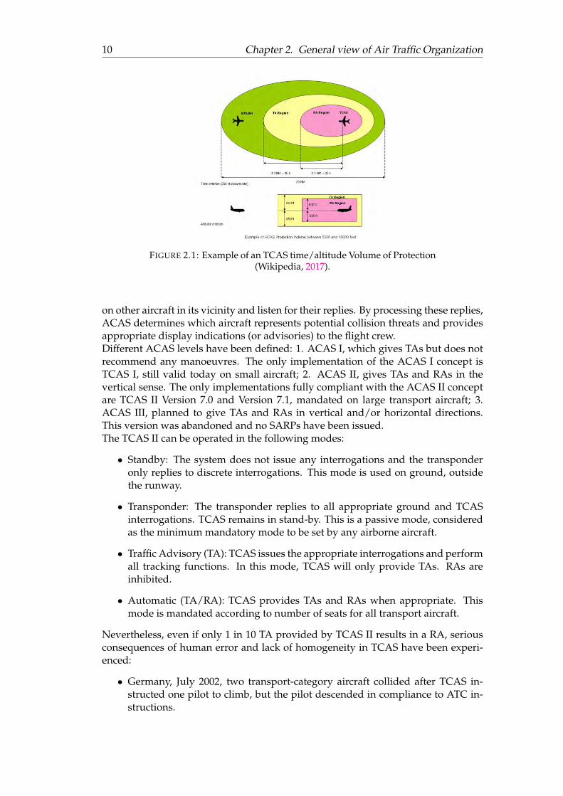
addition to this, it can address advisory services in non-controlled airspace.Depending on the type of flight and the class of airspace, ATC may provide instruc-tions that pilots are required to follow. On the other hand, ATC advisories (or flightinformation) can be neglected at the pilot’s discretion. Thus, even if the responsibil-ity for the safe operation of the aircraft is shared between ATC and the pilots, thefinal authority is the pilot in command, being able to deviate from ATC instructionsin an emergency to assure the safe operation of their aircraft.Concerning the separation between aircraft, mandatory rules are imposed for colli-sion prevention, assuring a minimum empty space around each aircraft at all times.In this manner, when a trajectory is planned for an aircraft, the uncertainty in thecomputation of future position of the aircraft is expressed in a "Volume of Protection"(VoP) around the estimated position of the aircraft, along with a level of confidencethat the aircraft will be within this VoP. Then, if no transgression between VoPs ofdifferent aircraft is found in the specified look-ahead time, it is considered that thereis no conflict for the planned trajectory (Suchkov, Swierstra, and Nuic, June 2003).The minimum size of this VoP is a circle of 2.5NM around the aircraft position, andthen, due to different longitudinal/lateral errors, an oval-shape bubble representinguncertainties is considered (Suchkov, Swierstra, and Nuic, June 2003). Also, it is of-ten considered that the longitudinal-track uncertainty increases with respect to thelook-ahead time.Current aircraft are equipped with collision avoidance systems that alert the pilotswhen other aircraft get too close. This is the case of the Traffic Alert and CollisionAvoidance Systems (TCAS), which is a specific implementation of the Airborne Col-lision Avoidance Systems (ACAS) concept developed by ICAO (ICAO 2006a). How-ever, not all TCAS systems can be considered as accepted ACAS.The TCAS II concept, for example, operates such that, when there is a reasonableconfidence that minimum separation standard (time-based) might become violatedin the near future, pilots are advised with tactical resolutions in order to avoid po-tential collisions (mid-air collisions and near mid air collisions). This is achievedthrough Resolution Advisories (RAs), which recommend actions (including ma-noeuvres), and through Traffic Advisories (TAs), which are intended to prompt vi-sual acquisition and to act as a precursor to RAs.An RA is generated nominally 15 to 35 seconds before the closest point of approachof the aircraft, and a TA from 48 to 20 seconds in advance of a RA. In Figure 2.1 isshown an example of the TCAS Protection Volume. Note that warning times dependon sensitivity levels of RAs.Consequently, it can be said that ACAS has been designed to provide a safety-net
collision avoidance service for the existing conventional air traffic control systems,while minimizing unwanted alarms in encounters where the collision risk does notneed escape manoeuvres. This system is based on Secondary Surveillance Radar(SSR) transponders, where three types of operation modes are available:
• Mode A: Transmission of 4 digit code on request.
• Mode C: Transmission of the standard barometric altitude on request.
• Mode S: Transmission of various parameters upon selective request. Coverageup to 120NM.
Since 1995, all Airbus aircraft are equipped with Mode S transponder, transmittingflight ID, altitude, and mode A code, and since 2001, all IFR aircraft in Europe arerequired to be equiped with mode S transponder.ACAS equipment in the aircraft interrogates Mode A/C and Mode S transponders
10 Chapter 2. General view of Air Traffic Organization
FIGURE 2.1: Example of an TCAS time/altitude Volume of Protection(Wikipedia, 2017).
on other aircraft in its vicinity and listen for their replies. By processing these replies,ACAS determines which aircraft represents potential collision threats and providesappropriate display indications (or advisories) to the flight crew.Different ACAS levels have been defined: 1. ACAS I, which gives TAs but does notrecommend any manoeuvres. The only implementation of the ACAS I concept isTCAS I, still valid today on small aircraft; 2. ACAS II, gives TAs and RAs in thevertical sense. The only implementations fully compliant with the ACAS II conceptare TCAS II Version 7.0 and Version 7.1, mandated on large transport aircraft; 3.ACAS III, planned to give TAs and RAs in vertical and/or horizontal directions.This version was abandoned and no SARPs have been issued.The TCAS II can be operated in the following modes:
• Standby: The system does not issue any interrogations and the transponderonly replies to discrete interrogations. This mode is used on ground, outsidethe runway.
• Transponder: The transponder replies to all appropriate ground and TCASinterrogations. TCAS remains in stand-by. This is a passive mode, consideredas the minimum mandatory mode to be set by any airborne aircraft.
• Traffic Advisory (TA): TCAS issues the appropriate interrogations and performall tracking functions. In this mode, TCAS will only provide TAs. RAs areinhibited.
• Automatic (TA/RA): TCAS provides TAs and RAs when appropriate. Thismode is mandated according to number of seats for all transport aircraft.
Nevertheless, even if only 1 in 10 TA provided by TCAS II results in a RA, seriousconsequences of human error and lack of homogeneity in TCAS have been experi-enced:
• Germany, July 2002, two transport-category aircraft collided after TCAS in-structed one pilot to climb, but the pilot descended in compliance to ATC in-structions.

2.1. Current Organization of Air Traffic 11
• Japan, January 2001, a Boeing 747 followed the ATC instruction to descend in-stead of the TCAS RA to climb, intersecting course with a McDonnell DouglasDC-10. The collision was avoided when the 747 was put into a steep descentafter visual contact with the other aircraft. About 100 crew and passengers onthe B747 sustained injuries due the emergency maneuver.
• Switzerland, June 2011, the crew from a Raytheon 390 followed an ATC de-scent clearance during their TCAS climb RA, creating a conflict with an Airbus319. Both aircraft passed in very close proximity (0.6 nm horizontally and 50feet vertically) without either seeing the other.
• Switzerland, May 2012, an Airbus 320 departing Zurich in a climbing turnreceived a TCAS RA to climb caused by an AW 139 only equipped with TCASI, also departing from Zurich. The conflict in Class C airspace was attributedto inappropriate clearance by the TWR controller and inappropriate separationmonitoring.
• May 2013, an Airbus 319 in Swiss Class C airspace received a TCAS RA tolevel off. This was due to a Boeing 737 located above, after being inadvertentlygiven an incorrect climb clearance by ATC.
The standardisation of ADS-B (Automatic Dependent Surveillance – Broadcast), TIS-B (Traffic Information Service - Broadcast), FIS-B (Flight Information Services - Broad-cast) messages, and their use on new Airborne Traffic Situational Awareness Ap-plications (ATSAW) (explained in Section 2.2.1), could lead to the replacement ofthe radar as a primary surveillance method. These broadcasts do not depend onany ground-based systems, but on transponders installed on the aircraft. This is asurveillance technique that relies on aircraft or airport vehicles broadcasting theiridentity, position, speed, altitude, heading and other information (ADS-B Out) de-rived from on board systems (e.g. GNSS). The transmitted signal can be captured forsurveillance purposes on the ground, or on board other aircraft (ADS-B In) in orderto facilitate airborne traffic situational awareness, and self-separation.The ADS-B is automatic because no external stimulus is needed. Therefore, the emit-ter has no knowledge of who receives the message due to the lack of interrogationor two-way contract. Also, the ADS-B is dependent because it relies on on-boardsystems. Moreover, wind estimations based on ADS-B data have been the subjectof recent research (Leege, Mulder, and Paassen, 2012), (Leege, Paassen, and Mulder,2013).
2.1.1.1.2 ATC units
The controlled airspace is divided into three ATC units in order to provide alertingservice and flight information service.
• Aerodrome control unit or Tower Control Unit (TWR): This unit controls flightsin the vicinity of aerodromes as well as traffic on the runway and taxiway. Inother words, it is in charge of the aircraft during landing and take-off phases.Visual contact with traffic is made from the TWR cab (see Fig. 2.2).
• Approach/Terminal Control Unit (APP)This unit controls arriving and departing aircaft in the Terminal ManoeuvringAreas (TMAs) and sometimes beyond (see Fig. 2.3). The area of responsibility

12 Chapter 2. General view of Air Traffic Organization
(a) TWR outside view. (b) TWR cab inside view.
FIGURE 2.2: Tower Control Unit (KLM, 2017).
of the APP is larger than that of the TWR. Approach controllers are respon-sible for sequencing arriving traffic for landing, and for providing separationbetween departing and arriving aircraft. The main tool of APP controllers isradar. In the United States of America, the APP is referred to as a TerminalRadar Approach Control (TRACON).
(a) Facility. (b) Air Traffic in a TMA.
FIGURE 2.3: Approach/Terminal Control Unit (StackExchange,2017a).
• Area Control Centre (ACC)Defined as a facility responsible for controlling en-route traffic in a definedvolume of airspace or FIR at high altitudes between airport approaches anddepartures. In USA, the ACC is referred to as an Air Route Traffic ControlCenter (ARTCC).
The APP (or TRACON) unit works between ACC (or ARTCC) and TWR (see Fig.2.4).
2.1.1.2 Air Traffic Flow and Capacity Management (ATFCM)
According to (ICAO July 2001[a]), ATFCM is a service in charge of managing a safe,orderly and expeditious flow of air traffic in order to avoid exceeding airport orair traffic control capacity, but ensuring that the maximum available capacity de-clared by the appropriate ATS authority is used efficiently. In other words, it aims tomeet traffic demand without overflowing airspace and/or aerodrome capacity, andif capacity is exhausted, rejects excess demand to maintain the maximum availablecapacity.

2.1. Current Organization of Air Traffic 13
FIGURE 2.4: Handling of Air Traffic (StackExchange, 2017b).
Since all aircraft using ATC need to file a flight plan and send it to a central repos-itory, air traffic flow and capacity computations are performed before flights. Ac-cording to (Eurocontrol, 2017a), the ATFCM activities are divided into three phases:
• Strategic Phase (1 year before flight - 1 week before time operations).The Network Operations Centre (NMOC), which manages one single flowmanagement system over Europe, helps the ANSPs to predict the capacitydemand for each ATC center. Then, a routing scheme is prepared such thatcapacity is maximized and air traffic is balanced. A Network Operations Plan(NOP) is issued.
• Pre-tactical Phase (6 days before time operations).The NMOC provides a daily plan optimising the ATM network performanceby minimising delays and costs. This plan is the result of Collaborative Deci-sion Making (CDM) processes, designed to ensure that affected stakeholders,service providers, and airspace users, can discuss capacity demands, flight ef-ficiency issues, and formulate plans considering all pertinent aspects. The out-put of this phase is an ATFCM daily plan (ADP), which can anticipate capacityshortfalls for certain ACCs/airports due to specific events such as large-scalemilitary exercises, sporting events, holidays, etc.
• Tactical Phase (the day of operations).The tactical phase consists of the monitoring and update of the Daily Planmade the day before, continuing to optimise capacity in order to minimise de-lays. Also, the flights of that day receive an individual departure time (slots).According to (Eurocontrol, 2017b), in order to avoid too many aircraft in the airat the same time and place, the NMOC calculates take-off times (CTOTs), alsoknown as slots. One slot is a period of time within which take-off has to takeplace (in Europe, 5 minutes before and 10 minutes after the CTOT). If, for somereason a slot is missed, the NMOC assigns a new one. Also, slot improvementscan be made to make use of the newly available capacity.
Both ATC sectors and airports have finite capacities and both are highly computer-ized for its regulation.Regarding airports, only one aircraft can land or take-off from a given runway at onemoment. In this manner, due to minimum separation distance or time to avoid col-lisions between planes, hourly capacities and aircraft delay computation are neededto evaluate the airport performance. Moreover, airport capacity varies throughoutthe day since it depends on several factors such as the number of runways, availabil-ity of ATC, layout of taxiways, weather, etc. In (FAA September 1983), computation

14 Chapter 2. General view of Air Traffic Organization
of airport capacity and aircraft delay for airport planning and design is stated, defin-ing properly the capacity as a measure of the maximum number of aircraft opera-tions which can be accommodated on the airport or airport component in one hour.On the other hand, capacity in an ATC sector is determined by the number of airtraffic controllers and complexity of the airspace under their control, such that oneaircraft may be subject to many restrictions such as changing routes instead of latedeparture, so no overflow of capacity in the departing airport, nor in the airspacesector is ensured. Nevertheless, time-critical flights (e.g. flights carrying human or-gans for organ transplantation) are exempted from such restrictions.Detailed information about the procedures and roles of the involved participants inthe ATFCM can be found in (Eurocontrol 2017g).
2.1.1.3 Air Space Management (ASM)
An airspace is defined as a portion of the atmosphere controlled by a country aboveits territory, including its territorial waters. Then, a controlled airspace is an airspacewhere air traffic control service is provided in accordance with the airspace classifi-cation.In Table 2.1, the airspace classification is described according to the Chapter 2, Ap-pendix 4 of (ICAO July 2001[a]). It is important to note that ICAO is a regulatorybody and not a direct ATC service. Thus, international air traffic control is delegatedto those nations who accept the responsibility for providing ATC services.The airspace classification assigns letters to each class. Classes from A to E are con-sidered as controlled airspace by an ACC, and F and G are uncontrolled airspace.However, since each national aviation authority determines how it uses the ICAOclassifications in its airspace design, the rules in some countries are modified so thatthey can fit the airspace rules and air traffic services that existed before the ICAOstandardisation. For example, class F is designed as an special airspace dependingon the country or region, which may not be always available.Figure 2.5 depicts these airspace classes at different altitudes Above Ground Level(AGL).In terms of normativity, (ICAO July 2005) is the guiding document when flying in
FIGURE 2.5: Classification of Airspace (FAA, 2017).
international airspace.In order to identify which country controls which airspace and determines whichprocedures needs to be used, ICAO divided the airspace of the world into FlightInformation Regions (FIRs), where one major ATC authority is identified with eachFIR.The FIRs may be subdivided into smaller Areas which can comprise from two tonine sectors. Each Area has enough controllers trained on all sectors in that Area.In sectors, they use distinct radio frequencies for communication with aircraft, and

2.1. Current Organization of Air Traffic 15
TABLE 2.1: Airspace Classification
Class Type offlight
Separationprovided Service provided Speed
limitationa
Radiocommunication
requirement
Subjectto ATC
clearance
A IFR only All aircraft ATC service N/A Continuoustwo-way Yes
IFR All aircraft ATC service N/A Continuoustwo-way Yes
B VFR All aircraft ATC service N/A Continuoustwo-way Yes
IFR IFR from IFRIFR from VFR ATC service N/A Continuous
two-way Yes
C VFR VFR from IFR
1. ATC service forseparation from IFR.2. VFR/VFR traffic
information (and trafficavoidance advice
on request)
Yes Continuoustwo-way Yes
IFR IFR from IFR
ATC service, trafficinformation about
VFR flights (and trafficavoidance advice
on request)
Yes Continuoustwo-way Yes
D VFR Nil
IFR/VFR andVFR/VFR
traffic information(and traffic avoidance
advice on request)
Yes Continuoustwo-way Yes
IFR IFR from IFR
ATC service and,as far as practical,traffic informationabout VFR flight
Yes Continuoustwo-way Yes
E VFR Nil Traffic informationas far as practical Yes No No
IFR IFR from IFRas far as practical
Ait trafficadvisory service;
Flight informationservice
Yes Continuoustwo-way No
F VFR Nil Flight informationservice Yes No No
IFR Nil Flight informationservice Yes Continuous
two-way No
G VFR Nil Flight informationservice Yes No No
a250knot IAS below 10,000ft AMSL (or FL100 when height of the transition altitude is lower).
each sector has a secure landline communication with adjacent sectors, approachcontrols, areas, ACCs, flight service centers, and military aviation control facilities.These landline communications are shared among all sectors that need them and areavailable on a first-come / first-served basis. Aircraft passing from one sector to an-other are handed off and requested to change frequencies to contact the next sectorcontroller.Concerning the sector boundaries, these are specified by aeronautical charts. Theusage of aeronautical charts allow pilots to know their location, topographic fea-tures, hazards and obstructions, navigation aids, navigation routes, landing areas,and other information such as radio frequencies and airspace boundaries.Moreover, specific types of charts are used depending on the phases of a flight. Ac-cording to (ICAO July 2001[b]), a rough and non extensive classification of charttypes is:
• World aeronautical
• Airport

16 Chapter 2. General view of Air Traffic Organization
• Terrain
• En-route
• Area/Sectional
• Standard Instrument Departure (SID)
• Standard Terminal Arrival Routes (STARS)
• Visual Approach
Examples of the aeronautical charts corresponding to the Toulouse area are shownin Figure 2.6. The charts used for IFR flights contain all relevant information aboutlocations of waypoints, or fixes. This is due to the lack of visual reference to theground, and therefore the need of pilots to rely on internal (GPS) or external (VOR)navigation aids. Moreover, the Victor airways defined as straight-line segments canbe appreciated in the figure.Special Areas of Operations (SAOs) can also be included in the aeronautical charts,
defined as permanent or temporary designated airspaces in which certain activitiesare confined, or areas where limitations are imposed to aircraft which are not part ofthose activities. These SAOs consist usually of:
• Prohibited areas (e.g. location of the White House)
• Military Operation Areas (MOAs)
• Military Training Route (MTR)
• Restricted areas (artillery firing, aerial gunnery, or guided missiles)
• Parachute jump aircraft operations
• Warning areas
• Alert areas
The traffic organization within airspaces can be split into en-route/oceanic and air-port/TMA.Concerning the en-route/oceanic airspaces, aircraft are expected to fly through thecenter line of airways or in a direct course between navaids. Each airway is based ona straight line at a certain Flight Level between fixed geographic coordinates of satel-lite navigation systems (GNSS), between two navigational aids (navaids), or at theintersection of two navaids. Commonly used navaids are the Very High Frequency(VHF) Omnidirectional Range (VOR) stations, Non Directional Beacons (NDBs) andDistance Measuring Equipment (DME). Airways possess a limited width used todefine the permitted navigation errors for each airway.On the other hand, en-route flights controlled by the ACCs, or arriving and depart-ing traffic in the TMAs, need to ensure a minimum separation distance betweenaircraft. According to the Chapter 5 of (ICAO July 2016), this separation distancevaries depending on the use of navaids, flight level, flight phase, etc.

2.1. Current Organization of Air Traffic 17
(a) High-altitude IFR en-route chart.
(b) Low-altitude IFR en-route chart.
(c) Sectional VFR chart for low levels.
FIGURE 2.6: Aeronautical charts (SkyVector, 2017).
2.1.2 Aeronautical Meteorology
A forecast is defined as the expected meteorological conditions for a specified areawithin a period of time. The organizations providing global weather forecasts are theEuropean Centre for Medium-Range Weather Forecasts (ECMWF) (ECMWF, 2017)and the USA National Center for Environmental Prediction (NCEP) (NOAA, 2017).The ECMWF’s forecasts cover time frames ranging from medium-range, to monthlyand seasonal, and up to a year ahead. The predictions describe the range of possiblescenarios and their likelihood of occurrence using their own atmospheric model anddata assimilation system, the Integrated Forecast System (IFS).

18 Chapter 2. General view of Air Traffic Organization
In parallel, the NCEP delivers weather, water, climate and space weather guidance,forecasts, warnings and analyses to its partners and external user communities. TheNCEP is divided in nine centers: Climate Prediction, Environmental Modeling, Na-tional Hurricane, NCEP Central Operations, Ocean Prediction, Space Weather Pre-diction, Storm Prediction, Weather Prediction, and the most relevant to this work,the Aviation Weather Center (AWC, 2017), which delivers consistent, timely and ac-curate weather information like aviation warnings and forecasts of hazardous flightconditions at all levels for the world airspace system. The model used for the NCEPis the Global Forecast System (GFS).According to Eurocontrol (Eurocontrol, 2017e), the meteorological service is pro-vided unlike any other within ATM systems. This is due to the division of responsi-bilities. Either a member state can provide MET services as an element in a portfolioof weather services, or it can have a service dedicated only to aviation meteorology.Thus, the MET service provider may be the meteorological service of a member state,a part of the national ANSP, military services, or a commercial provider of weatherservices.In the international field, the World Meteorological Organisation (WMO) is responsi-ble to meet the operational requirements stated by ICAO in (ICAO July 2007), whichis the annex describing the meteorological services that shall be provided by all des-ignated MET providers around the globe.Common information given by MET providers are the METAR/TAF, SIGMET andAIRMET. The METAR (METeorological Airport Report) is an observation report(not a forecast) containing data such as temperature, dew point, wind direction andspeed, precipitation, cloud cover and heights, visibility, and barometric pressure. Itcan also include precipitation amounts, lightning, Runway Visual Range (RVR) andother information.The complement to METARs are called TAF (Terminal Aerodrome Forecast), andthey report forecasted weather rather than current weather.The SIGMET (SIGnificant METeorologic information), advises of weather that is po-tentially hazardous to all aircraft: Severe Icing, Extreme Turbulence, Dust storms,low visibility to less than three miles and Volcanic Ash.Concerning AIRMET (AIRmen’s METeorological information), they advise of poten-tially hazardous weather that does not meet SIGMET criteria, for example:
• IFR or Mountain Obscuration
a Visibility less than three miles affecting more than 50% of the given area.
b Extensive mountain obscuration.
• Turbulence
a Continuous surface winds greater than 30 knots at the surface.
b Moderate Turbulence.
• Icing
a Freezing levels
b Moderate icing
In Figure 2.7, weather stations and SIGMET areas in Europe, as well as AIRMETareas in USA are shown.

2.1. Current Organization of Air Traffic 19
(a) AIRMETS in the US. 12 Dec 2017, 13hrs UTC
(b) SIGMETS and weather stations in Europe. 12 Dec 2017, 13hrs UTC
FIGURE 2.7: Common MET information (SkyVector, 2017).

20 Chapter 2. General view of Air Traffic Organization
2.2 Modern Air Traffic Organization
The expected growth of air traffic in the upcoming years has led to the need ofairspace optimization. An approach to this optimization is through the improve-ment of Area Navigation (RNAV) systems, such that flight crew and air traffic con-trollers need to know the on-board RNAV system performance capabilities of eachaircraft to determine if they fit into the new airspace requirements.RNAV is a method of navigation that allows aircraft to fly on a desired path withinthe coverage of ground navaids, and/or within the capability limits of self-containedaids. This navigation system may involve VORs and DMEs (Distance MeasurementEquipments), INS/IRU (Inertial Navigation System / Inertial Reference Unit), orsatellite systems (GNSS positioning) to determine the position of aircraft.However, since area navigation is based on the performance of available equipment,an alternative concept was introduced by ICAO in 2008, the Performance-BasedNavigation (PBN). PBN is based on the specification of performance requirementsfor aircraft navigating on an ATS route, on a terminal or approach procedure (ICAO2008). In other words, a shift from sensor-based to performance-based navigation iscarried on.The Performance-Based Navigation concept identifies 3 main components to re-spond to airspace requirements:
• Navigation Application: It refers to the application of the NAVAID infrastruc-ture with its associated Navigation Specification in ATS routes and instrumentflight procedures for an airspace concept. Considering an airspace concept asa general plan (in terms of safety, capacity, efficiency, environment and accessobjectives) for a particular airspace.
• NAVAID infrastructure: It refers to the ground (VOR and DME) and space(GNSS) navaids. The use of NDBs is excluded from PBN.
• Navigation Specification: It is a set of aircraft and air-crew requirements neededto support a navigation application within a defined airspace concept. Thereare two navigation specifications, the Area Navigation (RNAV) and the Re-quired Navigation Performance (RNP). The RNP specification requires on-board performance monitoring and alerting, and RNAV does not. Then, anRNAV system with an on-board performance monitoring and alerting capabil-ity, capable of achieving the performance requirement of RNP specifications, itis referred to it as a RNP system.
As stated before, modern aircraft equipped with RNAV capabilities allow aircraft tofly a chosen route within the navaids coverage, rather than flying from one navaidto another, like conventional navigation systems. However, the use of RNP systemsallows to monitor the navigation performance that is being achieved while inform-ing the crew about it. This on-board monitoring and alerting enhances the pilot’ssituational awareness, such that closer spacing from aircraft to aircraft without ATCintervention and reduced distances for obstacle clearance are achieved.The constraints associated to conventional, ground-based sensor specific routes /procedures, and the flexibility and benefits of performance-based, non-sensor spe-cific navigation, are shown in Figure 2.8.Each RNP and RNAV specification is designated in the form of RNP-X/RNAV-X,
where X denotes the lateral navigation accuracy in nautical miles. This means thatan aircraft following the specification must have the capability of remaining withinX nautical miles to the right or left side of the centerline with an accuracy of at least

2.2. Modern Air Traffic Organization 21
FIGURE 2.8: Comparison between Conventional, RNAV, and RNProutes.
the 95% (within 2σ in a normal distribution) of the flight time. The performance ofRNP systems is quantified by the Total System Error (TSE), which is given by
TSE =√NSE2 + FTE2 + PDE2 (2.1)
where the Path Definition Error (PDE), Navigation System Error (NSE), and theFlight Technical Error (FTE), can be seen in Figure 2.9.In terms of integrity, the probability that the TSE of each aircraft operating in RNPstays within the specified cross-track containment limit (expressed by±2xRNP) shallbe at least the 99.999% (within 4.4σ in a normal distribution) per flight hour for RNP,and 99.99999% (5.3σ) for RNP AR (RNP Authorization Required) (ICAO 2008).The navigation specifications for different flight phases is given by the tree in Fig-
FIGURE 2.9: Error definition in RNP.

22 Chapter 2. General view of Air Traffic Organization
ure 2.10. For arrival and departure trajectories on an aerodrome, RNP 1 or RNAV
Navigation Specifications
RNP Specifications
Designation RNP 0.3RNP 1RNP 2
RNP APCHRNP AR APCHAdvanced RNP
For otherflight phases
DesignationRNP 4
For oceanic and RemoteContinental Navigation
Applications
DesignationRNP
with additionalrequirements
to be determined(3D, 4D)
RNAV Specifications
DesignationRNAV 1RNAV 2RNAV 5
For en-routeand terminalnavigation
applications
DesignationRNP 10
For oceanic and RemoteContinental Navigation
Applications
FIGURE 2.10: Navigation specifications for different flight phases.
1 or 2 is planned according to traffic density, radar equipment and communicationresources, but the approach operations are divided in two specifications, the RNPAPCH and RNP AR APCH. According to (ICAO 2009), the RNP APCH is intendedfor general RNP requirements without operational authorization (up to RNP 0.3),and the RNP AR APCH demands a higher level of navigation performance (fromRNP 0.3 to RNP 0.1) in order to overcome issues of airport access in obstacle-richenvironments, facilitating ATM evolution. RNP AR APCH approach requires oper-ational authorization from the state regulatory authority.In the same way, it is important to include the key role that the expansion of GlobalNavigation Satellite Systems (GNSS) such as GPS (USA), BeiDou (China), Galileo(Europe), and Glonass (Russia), plays at the enhancement of the diversity of RNPand RNAV systems, as well as allowing an efficient use of airspace (route place-ment, fuel efficiency and noise abatement).According to (GSA, 2017), the performance of European GNSS is assessed by:
• Accuracy: Difference between the measured and real position, speed or timeof the receiver.
• Integrity: Capacity to provide confidence thresholds and alarms during anoma-lies in the positioning data.
• Continuity: Navigation system’s ability to function uninterruptedly.
• Availability: Time percentage where the signal is accurate, integral and contin-uous.
Furthermore, current expansions of GNSS can be categorized as:
• Satellite-Based Augmentation Systems (SBAS): Errors from GNSS are correctedin ground stations. Then, correction/information messages are broadcastedusing geostationary satellites to final users (aircraft), covering large areas andimproving performance of regular GNSS.
– Wide Area Augmentation System (WAAS) for North America.
2.2. Modern Air Traffic Organization 23
– Multi-functional Transport Satellite (MTSAT) and Multi-functional Satellite-based Augmentation System (MSAS) from Japan.
– European Geostationary Navigation Overlay Service (EGNOS) from Eu-rope.
– Global Positioning System (GPS) and Geostationary Earth Orbit (GEO)Augmented Navigation (GAGAN) from India.
– Systems under development:
∗ System of Differential Correction and Monitoring (SDCM) from Rus-sia∗ Beidou SBAS from China∗ KASS from South Korea∗ SBAS ASECNA from 17 African states
• Ground Based Augmentation Systems (GBAS): They provide augmentation toregular GNSS constellations at airport level, enhancing approach, landing, de-parture and surface operations. Position errors below 1m (1σ) in both horizon-tal and vertical axis are achieved. These systems broadcast correction messagesusing VHF radio datalink from ground transmitters, as an evolution of ILS (In-strument Landing System) and MLS (Microwave Landing System). In termsof landing performace2, primary GNSS with SBAS augmentation are limitedto CAT I approaches. On the other hand, GBAS allows CAT I, II and III ap-proaches. Global standards for GBAS CAT III validation were agreed in 2010and are expected to be ready in the 2015-17 timeframe.
• Aircraft Based Augmentation System (ABAS): They augment and/or integrateinformation obtained from other GNSS elements with available on-board in-formation.
In France, a schedule for the implementation of PBN operations is developped in(DGAC March 2012), where short, medium and long term goals are established.The short term goals (2012/2014) involve the following milestones: RNP 4 or RNAV10for oceanic operations and RNAV 5 for continental; Gradual implementations ofRNAV 1 for terminal operations; Gradual implementations of RNP APCH3 (foresse-ing to RNP AR APCH) for approach operations.
2Instrument approach operations are classified based on a designed lower operating minima. Be-low this minima, an approach operation shall only be continued with the required visual reference asfollows:
– Type A: A minimum descent height or decision height at or above 75m (250ft).
– Type B: A decision height below 75m. Type B approaches are categorize as:
∗ CAT I: A decision height not lower than 60m and with either a visibility not less than 800mor a RVR not less than 550m.
∗ CAT II: A decision height lower than 60m but no lower than 30m and RVR not less than300m.
∗ CAT IIIA: A decision height lower than 30m or no decision height and RVR not less than175m.
∗ CAT IIIB: A decision height lower than 15m or no no decision height and RVR less than175m but not less than 50m.
∗ CAT IIIC:no decision height and no runway visual range limitations.
CAT II and III instrument approach operations shall not be authorized unless RVR informationis provided.
3The RNP APCH, also called RNAV (GNSS), is associated to 4 type of approaches:
24 Chapter 2. General view of Air Traffic Organization
As medium term goals (2015/2019), the widescale deployment of RNAV1 for termi-nal operations, and the widescale deployment of RNP APCH and RNP AR APCHfor approach operations is planned, along with the initiation of advanced RNP.Finally, the long term objectives planned for the 2020 and after are: RNP 2 spec-ification for continental en-route operations and RNP 0.3 applicable to departure,en-route, and approach operations (developed mainly for helicopter operations);Definition of the Advanced RNP specification, whose objective is to enable variousrequirements (variable navigation details, capacity to make fixed radius turns, 4Dmanagement) for en-route, arrival, departure and approach requirements under asingle navigation specification; Introduction of new functionalities for RNP specifi-cations such as fixed radius turns (RF or Radius to Fix) in Terminal Areas, and FRT(Fixed Radius Transition) for the en-route phase.Currently, the French territory has RNAV 1 trajectories (PRNAV in Europe) availablein more than 75% of terminal zones of the DSNA.The expected benefits of the PBN concept through the navigation application are toprovide flexible routes and terminal procedures, reduce aviation congestion, con-serve fuel, reduce the impact of aircraft noise, improve safety and accessibility tochallenging airports, and increase airspace capacity, all of this while reducing oravoiding sensor-specific operations, routes and procedures and their associated costs.Moreover, the use of RNAV and RNP systems is clarified, such that the need of tac-tical ATC intervention is reduced dramatically, as the aircraft-to-aircraft separationis within the airspace design (Eurocontrol January 2013).All these benefits pointed out converge into the Freeflight concept, where the flight-crew is supposed to assure the separation from all known aircraft in accordance withapplicable airborne separation minima.
2.2.1 Freeflight
After the establishment of a Committee regarding the Future Air Navigation Sys-tems (FANS) in the early nineties, a new ATC method with no centralized controlwas proposed. This proposal, known as Freeflight, aimed to reduce the human fac-tor dependance, transferring more responsabilities to the growing technology, suchthat computers will ensure the required separation between aircraft.The main objective of the Freeflight concept is to allow aircraft flying under IFR tofollow their optimal route, while moving the responsibility of self-separation to theflight-crew, such that new procedures and rules of the air will be necessary, andground ATM components will be assigned a different role.This infers that the Freeflight concept requires a very high performance of aircraftnavigation systems in order to achieve a required level of safety, back-up proceduresmight be necessary for noncompliance scenarios.
• Non Precision Approach (NPA) with LNAV (Lateral Navigation) minima: Lateral guidancebased on ABAS reinforced GNSS signal is provided for final approach.
• Non Precision Approach (NPA) with LP (Localiser Performance) minima: Lateral guidancebased on SBAS reinforced GNSS signal is provided for final approach.
• Approach with vertical guidance of barometric type in final (APV Baro-VNAV) withLNAV/VNAV minima: Lateral guidance based on ABAS reinforced GNSS signal.
• Approach with SBAS type vertical guidance in final (APV SBAS) with LPV (Localiser Perfor-mance with Vertical guidance) minima: Lateral guidance based on SBAS reinforced GNSS sig-nal.
By the end of 2016, the DGAC expects to publish RNAV(GNSS) approaches over all controlled IFRaerodrome runway ends, including a certain number with vertical guidance (APV SBAS or APV Baro-VNAV).
2.2. Modern Air Traffic Organization 25
Concerning modern systems in charge of providing flight information of surround-ing traffic, and enabling the flight-crew to maintain separation of their aircraft fromone or more aircraft, ACAS versions like TCAS III and IV were abandoned. In spiteof the fact that these versions were capable to give Vertical and/or Horizontal di-rection as RAs, TCAS in its current form is not compatible with new operationalconcepts where spacing between aircraft is reduced, since superior technology hasmade TCAS approaches obsolete. Thus, the Airborne Separation Assistance System(ASAS) was proposed instead. The different ASAS application categories are:
• Airborne Traffic Situational AWareness applications (ATSAW): They only helpthe pilot to understand surrounding traffic.
• Airborne SPAcing applications (ASPA): Air Traffic Controllers are responsibleof separation between aircraft while demanding pilots to perform tasks to en-sure separation.
• Airborne SEParation applications (ASEP): Air Traffic Controller gives the sep-aration responsibility to the pilot for a limited time and only to one aircraft.
• Airborne Own-separation applications (AO): All pilots are responsible of theirown separation with respect to other aircraft. Air Traffic Controllers have noresponsibility, and indeed, they are not required. This is a highest autonomouslevel, corresponding to the Freeflight concept.
Therefore, the suggested strategy to avoid traffic conflicts in the modern air traf-fic organization is to maintain the self-separation trough the ASAS systems, and ifneeded, ACAS systems would provide a last-minute alert. In other words, the ASASassumes the responsibility of maintaining separation but the ACAS will remain asthe final conflict resolution resource.In this way, aircraft would operate with more and more autonomy when changingfrom one airspace to another, flying closer and assuring a safe distance with respectto other aircraft, provoking an enhancement of airspace capacity, safety and flexi-bility of air routes. It must be considered that the evolution from current controlledairspace to the airspaces where airborne self-separation is implemented will be grad-ually, hereby, special attention to transition areas is required. The expected evolutionof ATM after the Freeflight implementation in low density areas is focused in the dy-namic use of airspace, and then, in the implementation of the Freeflight concept inall domains.Currently, the Free Flight concept is implemented at Europe as a Free Route Airspace(FRA), where according to (Eurocontrol, 2017h), is a defined airspace where userscan freely plan a route from an entry to an exit point of the airspace, using publishedor unpublished waypoints for their routes (with no relation to ATS route networks).These routes are subjected to availability, and flights are subjected to air traffic con-trol. Besides, it is stated that flying distances caused by moving from routes to freeairspace can be reduced by 7.5 million NM, equivalent to 45,000 tons of fuel saved,or 37 million euros. Moreover, a FRA environment provides more stable trajectoriesand enhancement of conflict detection tools usage.Since the free routing across the European airspace represents a milestone on theroad to SESAR business trajectories and 4D profiles, a major part of the Europeanairspace is expected to have implemented FRA by the end of 2019 as a result ofcooperation between the ANSPs, airspace users, network managers, and militarypartners. In Figure 2.11 is shown the planned implementation of FRA in Europe,from a start in the summer of 2017 up to 2021/2022.

26 Chapter 2. General view of Air Traffic Organization
UDDDLIPPUBBALHCC
LHKR
LKAA
LSAZLFEE
LIMM
ESMMEVRR
LFRR
UKBV
LUUU
LMMM
GCCC
EETT
LBSR
EISN
EPWW
LFMM
EGTT
UGGG
LZBB
LYBA
ESOS
LJLA
LIBBLPPC
LFBB
EFIN
UKDV
UKOVLSAG
LOVV
LWSSLAAALECB
LRBB
LGGG
LDZO
UKLV
EYVC
LCCC
LGMD
EDUU
LIRR
LPPO
LECS
UKOVLFFF
UKDV
EDYY
EGPXRAW
LECMASU
LECMSAU
EGPXRAE
GMMMWESGMMMOCE
EGPXCEN
LECM
GMMM
LTAA
ENOR
ENOB
BIRD
EGPX
EKDK
Free Route Airspace ImplementationSummer 2017
Cross-Border ActivitiesFRA Plans to be updatedFRA (H24 / might be level restricted or on seasonal basis)FRA (Night / might be level restricted or on seasonal basis)DCT Comprehensive (H24)DCT Comprehensive (H24 partial AoR)DCT Comprehensive (Night and/or WE)DCT Limited (Night)
This map is for information purposes only.
© EUROCONTROL, November 2016
l
l
(a) Free Flight implementation in 2017.
EGPX
UDDDLIPP
EKDK
UBBALHCC
LHKR
LKAA
LSAZLFEE
LIMM
ESMMEVRR
LFRR LUUU
LMMM
GCCC
EETT
LBSR
EISN
EPWW
LFMM
EGTT
UGGG
LZBB
LYBA
ESOS
LJLA
LIBBLPPC
LFBB
EFIN
LSAGLOVV
LWSSLAAALECB
LRBB
LGGG
LDZO
EYVC
LCCC
LGMDLIRR
LPPO
LECS
LFFF
EDYY
UKBV
LECMASU
GMMMSOU
LECMSAU
GMMMNOR GMMMEAS
GMMMWESGMMMOCE
EDUUNorthEDUUEast
EDUUSouth
EDUUCentralWest
LECMLTAA
ENOR
ENOB
BIRD
Free Route Airspace ImplementationEnd 2021
Cross-Border ActivitiesFRA Plans to be updatedFRA (H24 / might be level restricted or on seasonal basis)FRA (Night / might be level restricted or on seasonal basis)DCT Comprehensive (H24)DCT Comprehensive (H24 partial AoR)DCT Comprehensive (Night and/or WE)DCT Limited (Night)
This map is for information purposes only.
© EUROCONTROL, November 2016
EDYY
EDUUCentralWest
EDWWEastEDMMEast
EDMMSouth
EDWW FL245 - FL285EDMM FL245 - FL315
BIA/Dl
l
(b) Free Flight implementation at the end of 2021.
FIGURE 2.11: Free Flight implementation (Eurocontrol, 2017i).

2.2. Modern Air Traffic Organization 27
2.2.2 SESAR and NextGen
According to (Eurocontrol, 2016), in 2012, 9.5 million flight were processed (0.7 bil-lion passengers), and for 2035, 14.4 million flights with 1.4 billion passengers areexpected. Furthermore, according to (Eurocontrol, 2017j), ATM in Europe handlesaround 26,000 flights daily, and by 2020, the traffic is expected to be doubled. Inaddition to this, the operating costs of ATM are rising at 2-3 billion euros per year.Therefore, the issue of improving the ATM performance while reducing operativecosts needs to be addressed.When this dramatic air traffic growth was detected, two projects were launched, oneby the U.S.A., and the other by the European Comission.In 2003, the Joint Planning and Development Office (JPDO) was established in or-der to provide a vision of the future U.S.A. air transportation system. The resultwas the Integrated National Plan for the Next Generation Air Transportation Sys-tem (better known as Next-Gen) in 2004, which defined the needed objectives andrequirements to improve the air transportation system (FAA, 2016). This projectinvolves several government agencies such as the FAA, NASA, Department of De-fense, National Weather Service, and the Transportation Security Administration,which released in 2007 the Next-Gen Concept of Operations, providing an overviewof the project goals for 2025.On the european side, a solution was launched by the European Commission in1999, under the idea to organize the airspace considering traffic flows instead of na-tional borders (FAB - Functional Airspace Block), giving birth to the Single EuropeanSky (SES).The current proposal of 9 FABs for the optimization of the European airspace is givenby (Eurocontrol, 2017k) as:
• FAB Europe Central (FABEC): France, Germany, Belgium, Netherlands, Lux-embourg and Switzerland (55% of flights through Europe pass over this airspace).
• FAB Central Europe (FABCE): Czech Republic, Slovak Republic, Austria, Hun-gary, Croatia, Slovenia, Bosnia and Herzegovina;
• North European FAB (NEFAB): Estonia, Finland, Latvia and Norway.
• South West FAB (SW FAB): Portugal and Spain.
• Baltic FAB: Poland and Lithuania.
• Danube FAB: Bulgaria and Romania;
• Denmark-Sweden FAB.
• UK- Ireland FAB.
• Blue Med FAB: Italy, Malta, Greece, Cyprus, as well as Egypt, Tunisia, Albaniaand Jordan as observers;
The primary goal of the SES was to provide the legislative framework required tocope with the capacity, environmental impact, and safety needs of future air traffic,foreseeing the improvement of current systems in the mentioned areas.Regarding the technological side of the SES, the Single European Sky ATM Research(SESAR) project was launched in 2004, in charge of the development and deploy ofthe necessary items to build the Europe’s future air transportation system. Threeyears later, a private-public partnership in the research and development sector of

28 Chapter 2. General view of Air Traffic Organization
ATM was founded by the European Union and Eurocontrol, named SESAR JointUndertaking (SESAR JU), encompassing 19 members representing over 100 compa-nies working towards the innovation of the ATM community.Some updated goals to be achieved by SESAR JU in the middle term (2009-2016)were to start the improvements concerning Continuous Descents and Climbs, taxi-ing, and CDM processes, and by the 2020 and further, depending on the availabilityof on-board equipment in aircraft, to introduce an optimized management of 4Dtrajectories (3D+T), autonomous self-separation of aircraft, and consequently, theredistribution of pilots/air traffic controllers/ machines roles. Yielding to a moreefficient air traffic management and reductions of CO2 emiisions (SESAR, 2017).These objectives are based on the Trajectory-Based Operations, which relies on theprovision of air navigation services (ANS) for business trajectories, and consistsof several ATM functions such as demand and capacity balancing, flexible use ofairspace, solution to air traffic conflicts, and tactical separation of aircraft, just tomention a few. In other words, the TBO concept allows aircraft to fly their preferredtrajectories without being constraint by airspace configurations.According to (ICAO, March 2014), a Business Trajectory is the preferred (optimal)profile for a flight determined by the aircraft operator. This trajectory is defined ina three dimensional flight profile with timestamps in specific points (4D), such thatATM constraints are meet. Prior to departure, a Shared Business Trajectory (SBT) issubmitted to ATM, and if agreed, it will become the Reference Business Trajectory(RBT). This RBT is updated and shared as required during the flight with every newmanoeuver resulting from the trajectory management loop between all ATM stake-holders. In other words, ideal TBO operates gate-to-gate using 4D trajectories formanage and control of airborne/ground operations. However, in (ICAO, July 2014),a not so radical 4D end-to-end trajectory is suggested, assuring that this would cre-ate a rigid non in-flight optimizable structure, incapable to respond to unpredictableelements such as capacity or weather. Alternatively, it is suggested the definition of"how to" and "how much" to optimize a trajectory depending on the type of con-straint.In the same tenor, since 4D trajectories are negotiated and updated between flightcrews and ATC, a shift from fixed routes and ATC clearances to flexible trajectories isinherent. Thus, higher levels of onboard automation are mandatory, while the lack ofdetailed aircraft parameters (usually known only on-board) become a reason for theSESAR TBO concept to support the use of ADS-C EPP (Extended Projected Profile).This is an improved version of ADS-C messages4. The EPP extends the trajectoryprediction beyond ANSP boundaries by reflecting the future trajectory predicted bythe FMS. Also, the EPP confirms that the aircraft’s FMS is consistent with any issuedlateral or vertical constraints and/or target time. In this manner, one reference tra-jectory and the corresponding flight information is shared between all ATM actors.More information regarding the sharing of trajectory predictions and time adher-ence in TBO, is available in (ICAO, October 2014[a]), (ICAO, October 2014[b]).Summarising, the general benefits of TBO can be stated as:
• Aircraft separation is reduced due to the decrease of uncertainty in the trajec-tories, thanks to higher guidance accuracy.
4ADS-C (Automatic Dependent Surveillance-Contract) operates similarly to ADS-B, but the data istransmitted based on an explicit contract (demand, periodic, event or emergency) between an ANSPand an aircraft. It is mainly used in the provision of ATS over transcontinental or transoceanic areas(low traffic levels)(SKYbrary, 2017).

2.2. Modern Air Traffic Organization 29
• An enhancement of capacity and efficiency in traffic flows within a given airspaceis assured since time-dependent reference trajectories are given.
• An optimal update of tactical trajectories due to weather or conflict avoidancecan be made since the reference trajectory is shared between all ATM actors.Since an optimal trajectory is more likely to be used, and they are usuallyshorter than the original path, reductions of CO2 emission and fuel burn areexpected.
• Flight predictability and safety are increased due to the use of GNSS and groundsystems.
2.2.2.1 Implementation of TBO
Continuous Descent and Continuous Climb Operations (CDO and CCO) are clearexamples of the use of TBO, where optimal flight paths are intended in order toachieve the best economic/environmental benefits (see Figure 2.12). These opera-tions could save from 50 to 200kg of fuel per flight using a single CCO or CDO,compared to a non-optimized profile (Eurocontrol, 2017l). Moreover, according to(NASA, 2013), data from the 27 busiest airports in the U.S.A. indicates that 188 mil-lion gallons of fuel per year could be saved with continuous climbs, and 218 millionwith continuous descents.CDO procedures were first evaluated at Louisville-Standiford International Airport,tested at Atlanta/Hartsfield-Jackson International Airport, and demonstrated at theMiami International Airport in May 2008. However CDO interaction with non-CDOflights, pilot adjustments to drag-generating devices (throttle changes, flap settings,landing gear extension), and further studies on the benefits of these operations, haveprovoked delays in their full implementation.On the other hand, CCOs are expected to be included as a part of a SID(StandardInstrument Departure), so ATC and flight crews have a fixed procedure defined inadvance.Ideally, CDOs use minimum engine thrust in a low drag configuration prior to land-ing, while CCOs use climb engine thrust and speeds until reaching cruise altitude(faster than step climbs). Both CDOs and CCOs are highly encouraged in Europe. Inconsequence, their associated ICAO manual have been issued, (ICAO 2010), (ICAO2013), respectively.
In addition to CCO and CDO techniques, 4D operations have been addressed inboth SESAR and Next-Gen projects, where the time integration as an extra dimen-sion to a 3D trajectory allows to consider delays as distortions from the referencetrajectory.The 4D concept relies on RBT (Reference Business Trajectory) that airspace userschoose to fly, and ANSPs to provide. This 4D (time-based) operations are consideredas milestones towards Trajectory-Based Operations due to their level of informationsharing between ATC and flight crews, as well as the required avionics, and requiredlevels of on-board automation.In the SESAR context, 4D trajectory management is divided in two stages, initial 4D(i4D), and Full 4D.The i4D consists in using airborne computed predictions in ground systems to de-fine a target time of arrival at a merging point to each aircraft converging to thispoint (e.g. Initial Approach Fix), such that traffic is sequenced. This implies fewertactical interventions and improved de-confliction situation.Although Controlled Time of Arrival (CTA) is a functionality available in modern

30 Chapter 2. General view of Air Traffic Organization
FIGURE 2.12: Concept of CDO (Eurocontrol October 2011).
Flight Management Systems, its use to improve efficiency in traffic management hasbeen explored only recently. According to (Klooster, Amo, and Manzi, 2009), thewind data available to the FMS, the speed and altitude constraints, and configura-tion for landing, are determinant factors that have a substantial impact on the CTAaccuracy. Therefore, higher wind modelling accuracy may considerably improve theaccuracy of the CTA operation.Implementation of the i4D was performed successfully the 10th February of 2012with an A320 test aircraft flying from Toulouse to Copenhagen, Stockholm, and thenback to Toulouse, underlying the datalink interoperability (exchange of trajectorypredictions between an advanced aircraft FMS and the ground automation systems)as a key element (Mutuel, Paricaud, and Neri, 2013), (SESAR Factsheet 2012).Regarding the Full 4D Trajectory Management concept of SESAR (4D gate-to-gate),it was initially planned to start the implementation between 2017 and 2019, but itwas delayed due to its impact on airborne and ground systems, as well as in theexistent procedures.In order to advance towards full 4D trajectories, some requirements for on-boardsystems and crew procedures need to be accomplished. For example: advanced fea-tures for FMS (improved wind modelling and update in the FMS), improved FMSability to meet time constraints, improvement of personalized, filtered, informationsharing like datalink (CPDLC and ADS-C EPP) for transmission of altitude, time,speed predictions, aircraft gross weight, etc., and introduction of SWIM (System-wide Information Management), just to mention a few.Moreover, considering that:
• Conflict detection is more complex since trajectories will no longer follow stan-dard airways, making conflicting points moving locations.
• TBO improvement in only a part of the trajectory will limit the benefit.
• Action of controllers will have an impact in the trajectory as a whole, since thereach of control points needs to be done in time and not later or earlier.
cost benefit analysis are being developed to ensure that costs associated with 4Davionics are justified by the potential benefits.
2.3. Conclusion 31
2.3 Conclusion
A summary regarding the current air traffic organization has been provided, describ-ing the main features of the CNS-ATM and MET services. Then, after recognizingthe imminent growth of air traffic, the solutions adopted by the European Unionand the United States of America were described as a part of a modern air trafficorganization.The advantages of a modern organization of air traffic have been pointed out, andthe gradual shift from fixed routes and ATC clearances towards flexible trajectories,higher levels of on-board automation, reduced aviation congestion, and improvedsafety, has been described.Moreover, the use of new technologies such as ADS-B/C, Global Navigation SatelliteSystems (GNSS), and their interaction with current ATM has also been described.Taking into account that the main goal of SESAR and Next-Gen projects is focusedon enhancing the airspace capacity while maintaining safety, the nearest concept tobe implemented is TBO, therefore, the Continuous Climb/Descent Operations andthe 4D concept are of great interest. This is expected since the Freeflight concept forhigh traffic regions will result in an increase of air conflicts, and automatic conflictresolutions may end in a permanent state of routes reconfiguration.Furthermore, certain similarities between the objectives of this thesis with respect tothe expected benefits of TBO are found.


33
Chapter 3
Flight Dynamics of TransportAircraft under Wind Disturbances
In this chapter, the nonlinear differential equations describing the behaviour of trans-port aircraft are described, such that they serve not only as a basis for further chap-ters, but also as a formal introduction for understanding the relation between dif-ferent frames, variables, and physical phenomena that contribute to explain aircraftflight. To begin with, an aircraft is considered as a rigid body with six degrees of free-dom (6 DOF) flying through a quasi-stationary flow field. The principal notation andnonlinear differential equations describing the aerodynamic forces and moments aswell as the motion of the aircraft are given based on (Etkin, 1972), (Etkin and Reid,1996), (Stevens and Lewis, 1992). This aircraft model hinges upon the Newton’s 2ndlaw.In Section 3.1, the reference frames and their respective rotation matrices betweeneach other are given. Then, Section 3.2 gives the rigid body equations, constructedby a set of nonlinear differential equations split into guidance and attitude dynam-ics. Moreover, a brief description of the aerodynamic force and moment coefficientsthat define the behaviour of the aircraft is provided. In spite of the fact that theseequations are called the complete mathematical model, some subsystems such asthe engines or the control surfaces are bypassed. Therefore, towards a more realisticapproach, first-order dynamics are proposed to govern the control surfaces and theengines. Besides, considering that some of the main disturbances during flights arecaused by wind gusts, it seems natural to take into account their effects while mod-elling the aircraft dynamics. In this manner, flight dynamics are expressed assumingwind contributions.Once the complete aircraft model is built up, it is a common practice in the litera-ture to simplify these equations into longitudinal and lateral motions, opening thedoor to a less complex analysis of flight mechanics. Stated this, one may infer thatthese simplified models are only valid for a limited domain of the behaviour of theaircraft. Thus, Section 3.3 presents the reduced equations of motion.In Section 3.4, an insight in aerodynamics regarding the force and moments coeffi-cients is provided to better understand the nature of the aircraft behaviour. Simul-taneously, it will serve as a basis for further chapters where numerical values areproposed for these coefficients. In addition to this, considering that transport air-craft are intended to look after passengers comfort, and structural limitations haveto be attended, the flight maneuvers are restricted by load factor boundaries. Hence,the relations to express the load factor depending on the aircraft variables are alsogiven in Section 3.5. Finally, a compilation of the relevant equations is presented inSection 3.6 for the reader’s convenience, and conclusions are given in Section 3.7.

34 Chapter 3. Flight Dynamics of Transport Aircraft under Wind Disturbances
3.1 Reference Frames
It is common to observe how not all variables are convenient to be expressed in onlyone reference frame, yielding to the choice of multiple frames to easily describe aphysical phenomena. In this work, only the necessary ones to express the aircraftdynamics are described.
3.1.1 Adopted frames
3.1.1.1 Inertial Frame
The inertial reference frame, represented by FI = (OI , xI , yI , zI), has the origin onthe center of the earth. The zI axis points north, the xI points towards the vernalequinox, and yI is perpendicular to both in a right-handed rotation. The WGS84(World Geodetic System) is considered. In the perspective of flight dynamics, sincethe relevant motions regarding dynamic stability have a very short duration com-pared to the motion of the earth itself, this frame is of minimal use, therefore will beignored.
3.1.1.2 Earth-fixed Reference Frame
The local earth reference frame is considered for the description of the trajectoriesthat an aircraft is flying, as well as the trajectories that the aircraft is supposed tofollow. This frame is denoted by FE = (OE , xE , yE , zE), and its origin is arbitrarilylocated on the ground. It is worth to say that the trajectory to be followed by theaircraft, referred to it as a 4D reference trajectory, is defined by three functions asso-ciated with the coordinates of the center of gravity of the aircraft supposed to followit. These functions are parameterized by time: xR(t), yR(t), zR(t), t ∈ [tinit, tend].
3.1.1.3 Body Reference Frame
A third reference frame is considered to represent the fast dynamics of the aircraft.It is attached to the body’s c.g. and is defined as FB = (C, xB, yB, zB), referred toit as the body frame. The xB axis goes from tail to nose of the aircraft while the zBaxis, perpendicular to the latter, points downwards and lies in the symmetry planeof the aircraft. To complete the triad, the direction of yB can be obtained by the crossproduct ~zB × ~xB . Figure 3.1 represents graphically the body and earth frame.
3.1.1.4 Stability Reference Frame
This frame, denoted by FS = (C, xS , yS , zS), has its axes chosen such that CxB isaligned with the aircraft velocity vector relative to the surrounding air mass (betterknown as airspeed, Va) by performing only a rotation around the yB axis.
3.1.1.5 Wind Reference Frame
Lastly, denoted by FW = (C, xW , yW , zW ), the wind frame is introduced since itallows to represent the aerodynamic forces on the aircraft. This frame has its xWaxis aligned with the airspeed. The difference between xB and xS , which is theprojection of xW in the CxBzB plane, gives birth to the angle of attack (α) (shortnotation: AoA). Also, the angle created by the projection of Va in the CxByB planeand the xB axis, is known as the sideslip angle (β). In the Figure 3.2 are represented

3.1. Reference Frames 35
FIGURE 3.1: Earth frame and Body frame.
the wind and stability frames with respect to the body frame.
FIGURE 3.2: Wind frame and Stability frame. AoA and Sideslip anglein the positive sense.

36 Chapter 3. Flight Dynamics of Transport Aircraft under Wind Disturbances
3.1.2 Rotation Matrices between frames
The interaction between different variables attached to different reference frames isdescribed mathematically thanks to the rotation matrices. These rotation matricesallow the mapping of variables from one frame to another. Consider the case ofmapping variables from the body frame into the wind frame, passing through thestability frame. This is done by making a rotation around two axes, denoted by xS
ySzS
=
cα 0 sα0 1 0−sα 0 cα
xByBzB
(3.1a)
xWyWzW
=
cβ sβ 0−sβ cβ 0
0 0 1
xSySzS
(3.1b)
Thus, in the inverse sense, physical quantities from the wind frame can be mappedinto the body frame by the following rotation matrix:
LBW =
cβ sβ 0−sβ cβ 0
0 0 1
cα 0 sα0 1 0−sα 0 cα
T
=
cαcβ −cαsβ −sαsβ cβ 0sαcβ −sαsβ cα
(3.2)
For more details on rotation matrices, see Appendix A.Therefore, in the case of the airspeed, which has only one component in the axes ofthe wind frame
(Vaw = [Va, 0, 0]T
), it can be represented in the body frame as
Vab = LBWVaw (3.3a)
Vab =
VacαcβVasβVasαcβ
(3.3b)
Moreover, if the wind components in the body frame are taken into account as Vw =[Vwx , Vwy , Vwz ]
T , the inertial velocity of the aircraft in the body frame is denoted by.
VB =
uvw
=
Vacαcβ + VwxVasβ + VwyVasαcβ + Vwz
(3.4)
Hence, the following relations are extracted from (3.4):
α = arctan
(w − Vwzu− Vwx
)(3.5a)
β = arcsin
(v − VwyVa
)(3.5b)
Va =√
(u− Vwx)2 + (v − Vwy)2 + (w − Vwz)2 (3.5c)
The vector R = [α, β, Va]T is defined for simplicity in further equations.
In the same tenor, the angles created from the difference between the body frameand the earth frame are the euler angles
(η = [φ, θ, ψ]T
), used to describe the atti-
tude of the aircraft.The euler angles are born as follows: It is a fact that the FB frame rotates, while FE

3.1. Reference Frames 37
is fixed, so the rotated frame FB can be imagined to be initially aligned with FE ,before undergoing three elemental rotations (rotations about the axes of a coordi-nate system) represented by the Euler angles. Any target orientation for FB can beachieved by composing three elemental rotations, these rotations occur around theaxes of the frame FB , attached to the moving body. Therefore, the rotation matrixfrom the body to the earth frame considering a rotation around the axes in the orderzByBxB , is given by:
LEB =
cθcψ sφsθcψ − cφsψ cφsθcψ + sφsψcθsψ sφsθsψ + cφcψ cφsθsψ − sφcψ−sθ sφcθ cφcθ
(3.6)
where the euler angles are bounded as φ−π, π; θ−π2 ,
π2 ; ψ−π, π, and limits are
never reached during normal operation for transportation aircraft.Consequently, the velocity of the aircraft in the earth frame is given by:
VE =
xE˙yE˙zE
= LEB
uvw
(3.7)
The rotation matrices used here belong to the SO3 group. Thus, the inverse of anyof these matrices equals to its transpose.

38 Chapter 3. Flight Dynamics of Transport Aircraft under Wind Disturbances
3.2 Equations of motion
The four principal forces on an aircraft are shown in Figure 3.3, where the Thrust(Fthr) is provided by the engines in the opposite direction of the Drag (D), and theWeight of the aircraft (W ) is compensated by the Lift (L).Lift and Drag of the wing are assumed to act in the wing’s pressure center, so that
FIGURE 3.3: Forces acting on an aircraft.
if a frame has its origin in this point of the aircraft, the pitching moment is equalto zero. This decision is far from being the optimal due to the changing locationof the centre of pressure along the wing as the angle of attack changes. In order toavoid this problem, a point called aerodynamic center (a.c.) is defined, where thepitching moment is almost invariant relative to the AoA variation (within permittedlimits). In subsonic velocities (Mach<1), the a.c. is at 1/4 of the wind chord, whichis geometrically forward the centre of pressure, such that if a frame is chosen withits origin in the a.c., it will cause an approximately constant nose-down (negative)moment relative to the AoA positive variation when static stability is positive. Asthe the center of gravity (c.g.) of the aircraft moves ahead the a.c., the more positivestatic stability is obtained.Therefore, considering the body frame attached to the c.g. of the aircraft, the equa-tions of motion are split into guidance equations, assumed to be the slow dynamics,and in attitude equations, considered as the fast dynamics. Moreover, first ordermodels for the actuators are considered.
3.2.1 Guidance Dynamics
Considering the Newton’s 2nd law with fE as the resultant force acting on the air-craft, one should obtain the external and internal forces acting on the aircraft. How-ever, the internal forces (those exerted by one small aircraft’s mass element upon an-other), all occur in equal and opposite pairs, such that by Newton’s third law, theycontribute nothing to the resultant force. Consequently, fE is the resultant externalforce acting on the aircraft, and it is obtained by:
fE = mVE (3.8a)
LEBfB = md
dt(LEBVB) = m
(LEBVB + LEBVB
)(3.8b)

3.2. Equations of motion 39
Then, denoting the angular rates by Ω = [p, q, r]T , the Euler property is given by
LEB = LEBΩ = LEB
0 −r qr 0 −p−q p 0
(3.9)
Therefore, (3.8b) can be rewritten as
fB = m(VB + Ω× VB
)(3.10)
where m is the aircraft mass, and fB is the vector of external forces in the body frame,conformed by the aerodynamic forces, the thrust, which is assumed to be alignedwith the xB axis, and the gravitational force projected in the body frame, yielding
fB = mLBE
00g
+
FxaFyaFza
+
Fthr00
(3.11)
where the aerodynamic forces, generated in the wind frame as Lift, Drag, and Side-force (Y ), are denoted in the body frame using (3.2) such that Fxa
FyaFza
= LBW
−DY−L
(3.12)
which are simultaneously related with their aerodynamic force coefficients by: DYL
=1
2ρSV 2
a
CDCYCL
(3.13)
with ρ as the air density and S wing area. Some authors prefer to use the free-streamdynamic pressure, denoted by q = 1
2ρV2a . However, the full notation will be kept in
this work. The aerodynamic force coefficients CD,Y,L will be addressed later.Thus, an acceleration equation in the body frame using (3.10) and (3.11) is denotedby: u
vw
=
1m (Fxa + Fthr)− gsθ + rv − qw
1mFya + gcθsφ + pw − ru1mFza + gcθcφ + qu− pv
(3.14)
While in the Earth frame, (3.8a) is rewritten as: xEyEzE
= LEB
Fxa + FthrFyaFza
1
m+
00g
(3.15)
3.2.2 Attitude Dynamics
Concerning the attitude of the aircraft, the angular rates are produced by the deflec-tion of ailerons, elevator and rudder, denoted by [δail, δele, δrud]
T . Hence, the totalangular momentum hE (not the same as moment) with respect to the aircraft’s c.g.needs to be obtained, since this quantity remains constant unless an external mo-ment actuates on the aircraft. For a moving point other than the mass center, the

40 Chapter 3. Flight Dynamics of Transport Aircraft under Wind Disturbances
following equations do not apply.Using a similar argument to that used for the forces, the total angular momentumis shown to be the resultant external moment about de aircraft’s c.g., and it is relatedwith the rolling, pitching and yawing aerodynamic moments (Mext = [L′,M,N ]T )by
MextE = hE (3.16a)
LEBMext =d
dt(LEBhB) = LEBhB + LEBhB (3.16b)
Knowing that hB = IΩ, and that I stands for the inertia matrix, assumed to beconstant, with some components equal to zero due to the aircraft symmetry, anddenoted by
I =
A 0 −E0 B 0−E 0 C
(3.17)
equation (3.16b) can be written as
Mext = IΩ + Ω× (IΩ) (3.18)
Then, rearranging for the angular rates like in (Lombaerts et al., May-June 2009), therotational equations of the aircraft can be expressed by:
Ω = I−1Mext − I−1Ω× (IΩ) (3.19)
with
I−1 =1
B(AC − E2)
BC 0 BE0 AC − E2 0BE 0 AB
(3.20)
It is known that the aerodynamic moments are dependent in part on the deflectionof control surfaces, aircraft velocity, air density, and other parameters such as certainaerodynamic moment coefficients. The relations for these aerodynamic moments aregiven by:
Mext =
L′
MN
=1
2ρSV 2
a
bClcCmbCn
+ Cδ
δailδeleδrud
(3.21)
where
Cδ =
bClδail 0 bClδrud0 cCmδele 0
bCnδail 0 bCnδrud
(3.22)
with b as the wingspan and c as the mean chord. The rolling, pitching and yawingaerodynamic moment coefficients (Cl, Cm, Cn, respectively) are denoted by: Cl
CmCn
=
Clββ + Clpbp
2Va+ Clr
br2Va
Cm0 + Cmαα+ Cmqcq
2Va
Cnββ + Cnpbp
2Va+ Cnr
br2Va
(3.23)

3.2. Equations of motion 41
where Clβ,p,r,δail,δrud , Cm0,α,q,δele, Cnβ,p,r,δail,δrud , will be addressed later.
Then, equation (3.19) can be rewritten using (3.21) as
Ω = I−1
1
2ρV 2
a S
bClcCmbCn
+ Cδ
δailδeleδrud
+
(B − C)qr + Epq(C −A)pr − E(p2 − r2)
(A−B)pq − Erq
(3.24)
or in a compact form by introducing (3.20) as
Ω =1
B(AC − E2)
BC 0 BE0 AC − E2 0BE 0 AB
(B − C)qr + Epq + L′
(C −A)pr − E(p2 − r2) +M(A−B)pq − Erq +N
(3.25)
Moreover, the rotation speed components are related with the attitude angular ratesby the Euler equations, given by: φ
θ
ψ
=
1 tgθsφ tgθcφ0 cφ −sφ0
sφcθ
cφcθ
pqr
(3.26)
Positive sense of forces, moments and velocities can be seen in Figure 3.4.
FIGURE 3.4: Positive sense of velocities and aerodynamic forces andmoments.

42 Chapter 3. Flight Dynamics of Transport Aircraft under Wind Disturbances
3.2.3 Dynamics in the wind frame
In order to express the flight dynamics in the wind frame, (3.5a) is differentiated,and using (3.4), (3.12), (3.14), the rate of change of the AoA is given by:
α =(u− Vwx)(w − Vwz)− (w − Vwz)(u− Vwx)
(u− Vwx)2 + (w − Vwz)2
=1
Vacβ
[cα(w − Vwz)− sα(u− Vwx)
]=
1
Vacβ
(g1 −
1
m(L+ Fthrsα)
)+ p
(−tanβcα −
Vwycα
Vacβ
)+ q
(1 +
Vwxcα + VwzsαVacβ
)+ r
(−tanβsα −
Vwysα
Vacβ
)+
1
Vacβ
(Vwxsα − Vwzcα
)(3.27)
with:
g1 = g (cαcθcφ + sαsθ)
Similarly, differentiating (3.5b), and using (3.4), (3.12), (3.14), the rate of change ofthe sideslip angle is given by:
β =Va(v − Vwy)− (v − Vwy)VaVa√V 2a − (v − Vwy)2
=cβ(v − Vwy)− cαsβ(u− Vwx)− sαsβ(w − Vwz)
Va
=1
Va
(g2 +
1
m(Y − Fthrcαsβ)
)+ p
(sα +
Vwzcβ + Vwysαsβ
Va
)+ q
(Vwzcαsβ − Vwxsαsβ
Va
)+ r
(−cα −
(Vwycαsβ + Vwxcβ)
Va
)+
1
Va
(Vwxcαsβ − Vwycβ + Vwzsαsβ
)(3.28)
with:
g2 = g (cβcθsφ + sβcαsθ − sαsβcθcφ)
Then, from (3.5c), and using (3.4), (3.12), (3.14), it is obtained:
Va =(u− Vwx)(u− Vwx) + (v − Vwy)(v − Vwy) + (w − Vwz)(w − Vwz)
Va
= g3 +1
m(Fthrcαcβ −D) + p
(Vwzsβ − Vwysαcβ
)+ q (Vwxsαcβ − Vwzcαcβ)
+ r(Vwycαcβ − Vwxsβ
)− Vwxcαcβ − Vwysβ − Vwzsαcβ (3.29)
with:
g3 = g (−cαcβsθ + sβcθsφ + sαcβcθcφ)
The expression in matrix form of relations (3.27), (3.28) and (3.29), rearranged for Ωis denoted by: α
β
Va
=
H11 H12 H13
H21 H22 H23
H31 H32 H33
pqr
+
Q1
Q2
Q3
(3.30)

3.2. Equations of motion 43
where
H11 = −(tanβcα +
Vwycα
Vacβ
)H12 = 1 +
Vwxcα + VwzsαVacβ
H13 = −(tanβsα +
Vwysα
Vacβ
)H21 = sα +
Vwzcβ + Vwysαsβ
Va
H22 =Vwzcαsβ − Vwxsαsβ
Va
H23 = −(cα +
Vwycαsβ + Vwxcβ
Va
)H31 = Vwzsβ − VwysαcβH32 = Vwxsαcβ − VwzcαcβH33 = Vwycαcβ − Vwxsβ
Q1 =1
Vacβ
(g1 −
1
m(L+ Fthrsα)
)+
1
Vacβ
(Vwxsα − Vwzcα
)Q2 =
1
Va
(g2 +
1
m(Y − Fthrcαsβ)
)+
1
Va
(Vwxcαsβ − Vwycβ + Vwzsαsβ
)Q3 = g3 +
1
m(Fthrcαcβ −D)− Vwxcαcβ − Vwysβ − Vwzsαcβ
which can be written as:R = H (R) Ω +Q (R) (3.31)
It can be easily verified that if the wind components are zero, the equations (3.27),(3.28) and (3.29) take the form:
α = q − tan(β) (pcα + rsα) +1
Vacβ
[g1 −
1
m(L+ Fthrsα)
](3.32a)
β = psα − rcα +1
Va
[1
m(Y − Fthrcαsβ) + g2
](3.32b)
Va = g3 +1
m(Fthrcαcβ −D)
(3.32c)
3.2.4 Actuator Dynamics
Let a first-order model be adopted for the aerodynamic actuators, writing δdi (i =ail, ele, rud) as the commanded positions of the control surfaces, and δi as the currentpositions of the control surfaces:
δi =1
ξi
(δdi − δi
)(3.33)

44 Chapter 3. Flight Dynamics of Transport Aircraft under Wind Disturbances
where ξi are the time-constants. Also, the resultant thrust produced by the enginesis supposed to behave as a first-order system, denoted by
Fthr =1
ξT
(F dthr − Fthr
)(3.34)
where the F dthr is the desired thrust and Fthr the current thrust. Besides, the time-constants of the actuators keep the relation: ξT >> ξi .

3.3. Reduced equations of motion 45
3.3 Reduced equations of motion
Nowadays, the Flight Management System is in charge of designing the route that anaircraft is going to fly from the departure airport to the arrival airport, better knownas the flight plan (Walter, 2014). The resultant flight plan, constructed from way-points, bearings, geographical locations or distances inserted by the crew, is createdin two separate plans, the lateral and vertical. Consequently, it is a common practiceto split the complete aircraft dynamics in longitudinal and lateral-directional mo-tions, such that flight controls are also separated. The longitudinal motion is used tofollow the vertical flight plan, and the lateral-directional to follow the lateral flightplan.By splitting the aircraft dynamics, there is the advantage of reducing the numberof nonlinear differential equations describing either the longitudinal or lateral be-haviour. On the other hand, the natural coupling of both motions is lost (for a nonsymmetric flight situation). It is also interesting that for steady level flight, climbing,or descending, the lateral dynamics are decoupled from the longitudinal dynamics,reducing considerably the complexity of the equations of motion.
3.3.1 Longitudinal Motion
In order to obtain the longitudinal equations, given by the movement in the CxBzBplane, some assumptions have to be made. It is assumed that the sideslip angle iszero, as well as the bank angle, consequently, the angular rates p and r are inexistentand the pitch rate is given by the reduction of equation (3.26) as
θ = q (3.35)
Moreover, from (3.25) it is obtained that
q =M
B(3.36)
Applying these considerations to equations (3.27) and (3.29), and introducing theFlight Path Angle (f.p.a.), depicted in Figure 3.5 and denoted by
γ = θ − α (3.37)
the vertical motion in the wind frame is given by:
FIGURE 3.5: Flight Path Angle.
46 Chapter 3. Flight Dynamics of Transport Aircraft under Wind Disturbances
γ =1
mVa(L+ Fthrsα −mgcγ)− q
(Vwxcα + Vwzsα
Va
)+
1
Va
(Vwzcα − Vwxsα
)(3.38a)
Va =1
m(Fthrcα −D −mgsγ) + q (Vwxsα − Vwzcα)− Vwxcα − Vwzsα (3.38b)
Furthermore, (3.2) becomes
LBW =
cα 0 −sα0 1 0sα 0 cα
(3.39)
Therefore, it is extracted from (3.12) that[FxaFza
]=
[Lsα −Dcα−Lcα −Dsα
](3.40)
and consequently, from substituting (3.40) in (3.14), it is obtained
u =1
m(Fthr + Lsα −Dcα)− gsθ − qw (3.41a)
w = − 1
m(Lcα +Dsα) + gcθ + qu (3.41b)
In the same way, considering φ = 0 in (3.6), the following relations are extractedfrom (3.7):
xE = ucθcψ + wsθcψ (3.42a)zE = −usθ + wcθ (3.42b)
Then, if β = 0 in (3.4), it is obtained that
u = Vacα + Vwx (3.43a)w = Vasα + Vwz (3.43b)
Thus, if (3.42) and (3.43) are combined, yields
xE = Vacψ(cαcθ + sαsθ) + Vwxcθcψ + Vwzsθcψ (3.44a)zE = Va(sαcθ − cαsθ)− Vwxsθ + Vwzcθ (3.44b)
which can be rewritten using the f.p.a. γ as
xE = Vacγcψ + Vwxcθcψ + Vwzsθcψ (3.45a)zE = −Vasγ − Vwxsθ + Vwzcθ (3.45b)
It can be easily verified that if the wind components are neglected, (3.38a) and (3.45)are reduced to
γ =1
mVa(L+ Fthrsα −mgcγ) (3.46a)
Va =1
m(Fthrcα −D −mgsγ) (3.46b)
xE = Vacγcψ (3.46c)zE = −Vasγ (3.46d)

3.3. Reduced equations of motion 47
One last generalization can be pulled of the longitudinal equations, this is when theaircraft is flying at constant altitude.
3.3.1.1 Level Flight
Assume that the aircraft is flying at constant altitude, hence, the f.p.a. dynamics arezero. In consequence, from (3.46a) and (3.46b) is obtained that
mg = Fthrsα + L (3.47a)
Va =1
m(Fthrcα −D) (3.47b)
and, if the velocity is assumed constant
Fthrcα = D (3.48)
3.3.2 Lateral-directional Motion
Moving on to the lateral equations, given by the movement in theCxByB plane, theyare obtained by assuming that θ = q = 0, such that from (3.26) it is obtained that
φ = p (3.49a)
ψ = rcφ (3.49b)
and from (3.25)
p =1
AC − E2
(CL′ + EN
)(3.50a)
r =1
AC − E2
(EL′ +AN
)(3.50b)
Therefore, under these assumptions, the lateral motion in the wind frame is givenby the reduction of (3.28) as
β =1
Va
(g (cβsφ − sαsβcφ) +
1
m(Y − Fthrcαsβ)
)+ p
(sα +
Vwzcβ + Vwysαsβ
Va
)+ r
(−cα −
(Vwycαsβ + Vwxcβ)
Va
)+
1
Va
(Vwxcαsβ − Vwycβ + Vwzsαsβ
)(3.51)
Furthermore, since the rotation matrix LBW remains as (3.2), the aerodynamic forceobtained from (3.12) is expressed by
Fya = −Dsβ + Y cβ (3.52)
Then, substituting (3.52) in (3.14) yields to
v =1
m(−Dsβ + Y cβ) + gsφ + pw − ru (3.53)
In this manner, if φ = 0 in (3.6), it is extracted from (3.7) the relation:
yE = ucθsψ + vcψ + wsθsψ (3.54)
48 Chapter 3. Flight Dynamics of Transport Aircraft under Wind Disturbances
and substituting (3.4) in (3.54), considering β = 0 yields to
yE = Vasψ (cθcα + sθsα) + Vwxcθsψ + Vwycψ + Vwzsθsψ (3.55)
Finally, if the wind components are neglected, (3.51) and (3.55) turn into
β =1
Va
(g (cβsφ − sαsβcφ) +
1
m(Y − Fthrcαsβ)
)+ psα − rcα (3.56a)
yE = Vacγsψ (3.56b)
One last generalization of the lateral movement is when the transport aircraft per-form equilibrated turns.
3.3.2.1 Steady turn
Considering that the aircraft is turning at constant altitude with a non-zero headingrate, the body-axis angular rates are given by:
Ω =
pqr
= LBE
00
ψ
(3.57)
and the AoA, sideslip angle, and the wind components are zero. It is obtained from(3.4) that VB = [u, v, w]T = [Va, 0, 0]T . Thus, from the force equations in yB given by(3.14), if is considered that the aerodynamic force is zero, the expression
v =1
mFya + gcθsφ + pw − ru (3.58)
turns intosφ =
Var
gcθ(3.59)
In consequence, using the yaw rate of (3.57), the heading rate is obtained:
ψ =g
Vatanφ (3.60)
This relation denotes how banked turns can be performed through the coupling ofrolling and yawing motions. Moreover, since banked turns can be performed eitheras a coordinated turn (coordination of the ailerons and rudder), or uncoordinatedturn (skidding or sliding turn), a brief analysis about this subject is provided later.

3.4. Dimensionless Aerodynamic Coefficients 49
3.4 Dimensionless Aerodynamic Coefficients
In Section 3.2, the equations (3.13) and (3.21) were given to describe the aerodynamicforces and moments. D
YL
=1
2ρSV 2
a
CDCYCL
and L′
MN
=1
2ρSV 2
a
bClcCmbCn
+ Cδ
δailδeleδrud
where
Cδ =
bClδail 0 bClδrud0 cCmδele 0
bCnδail 0 bCnδrud
These aerodynamic forces and moments, can be expressed in terms of the dimensionalstability derivatives (also called aerodynamic derivatives), which are the changes of anaerodynamic force or moment due to a motion variable like (u, v, w, p, q, r). In ad-dition to this, the dimensional stability derivatives are expressed in terms of nondi-mensional stability derivatives, which are the partial derivatives of the force or mo-ment aerodynamic coefficients with respect to a nondimensional motion quantity(u, v, w, p, q, r). These nondimensional quantities are given by (Etkin and Reid, 1996)as
u = uVa
v = vVa
w = wVa
p = pb2Va
q = qc2Va
r = rb2Va
An example to clarify this is provided for the aerodynamic rolling moment L′ =12ρV
2a SbCl. Note that the aerodynamic moments generated by the ailerons and ruder
are neglected for the example. Thus, the rolling moment is expressed using thedimensional stability derivatives as
L′ = L′vv + L′pp+ L′rr (3.61)
where the derivative L′r, for example, represents the change in the rolling momentdue to the angular velocity r, given by the partial derivative
L′r =∂L′
∂r=
1
2ρV 2
a Sb∂Cl∂r
(3.62)
Thus, considering that the partial derivative can be expressed in terms of a nondi-mensional quantity, if the expression for r = rb/2Va is included (hence ∂r = 2Va
b ∂r),(3.62) is rewritten using Clr = ∂Cl
∂r as
L′r =1
4ρVaSb
2Clr (3.63)

50 Chapter 3. Flight Dynamics of Transport Aircraft under Wind Disturbances
Analogously for the other dimensional derivatives, it is obtained that
L′v =1
2ρVabSClβ (3.64a)
L′p =1
4ρVab
2SClp (3.64b)
L′r =1
4ρVab
2SClr (3.64c)
whereClβ , Clp andClr are the nondimensional stability derivatives. Therefore, (3.61)is rewritten as
L′ =1
2ρV 2
a Sb
(Clβ
v
Va+ Clp
pb
2Va+ Clr
rb
2Va
)(3.65)
leading to an expression of the form
L′ =1
2ρV 2
a SbCl (3.66)
where
Cl =
(Clβ
v
Va+ Clp
pb
2Va+ Clr
rb
2Va
)(3.67)
Then, considering that β = vVa
by linearizing (3.5b), and neglecting wind effects, it isobtained that
Cl =
(Clββ + Clp
pb
2Va+ Clr
rb
2Va
)(3.68)
In this manner, when the same logic is applied for all the aerodynamic moments, theexpression (3.23) is found, denoted by Cl
CmCn
=
Clββ + Clpbp
2Va+ Clr
br2Va
Cm0 + Cmαα+ Cmqcq
2Va
Cnββ + Cnpbp
2Va+ Cnr
br2Va
On the other hand, when the same process is followed for the aerodynamic forces,it is found that the main contribution for the Lift coeficient CL is given by the AoA(CLα), for the Sideforce coefficient is the sideslip angle (CYβ ), and the Drag coeffi-cient is obtained from the Lift coefficient. This is denoted by: CL
CYCD
=
CLααCYββ
CD(CL)
(3.69)
where each nondimensional stability derivative contribution is briefly explained inthe next chapter, along with numerical values used for the simulation of a 6DOFtransport aircraft.

3.5. Load factor 51
3.5 Load factor
The load factor, commonly expressed in g units, refers to the fact that an observeron board an aircraft will experience an apparent acceleration of gravity relative toits frame of reference. For example, an observer on board an aircraft performing aturn with a load factor of 2, i.e., a 2g turn, will see objects falling to the aircraft floorat twice the normal acceleration of gravity. Consequently, the observer will have anapparent weight of twice his actual weight.Since transport aircraft are designed to flight smooth trajectories, some limitationson the load factor have to be respected for the well being and comfort of passen-gers. According to (FAA May 2017), on a typical flight, the load factor is limited to+2.5g and -1g for regular maneuvers, or up to 3.8g in maximum takeoff weight. Theexpressions for the load factor (in the body frame) of an aircraft are given by
ncg =1
mgWapp =
1
mg
mg −sθcθsφcθcφ
+mVB × Ω
(3.70)
where Wapp is the apparent weight of the aircraft. Some relations can be extractedfrom assumptions on these equations. The case of a steady turn is considered first.Thus, rewriting (3.70) in a scalar form yields to
nx = −sθ +(rv − qw)
g(3.71a)
ny = cθsφ +(pw − ru)
g(3.71b)
nz = cθcφ +(qu− pv)
g(3.71c)
Separately, under the assumptions of a steady turn given by (3.57), it was obtainedthe relation (3.60). This relation can also be obtained by assuming ny = 0 and using(3.57).Hence, using (3.57) and (3.60) in (3.71c), it is obtained that
nz =cθcφ
(3.72)
Note that the bigger value of nz is obtained when θ = 0. In this way, the maximumbank angle before reaching a 2.5g limit is 66.5.Another analysis that can be done is the one involving the centrifugal acceleration(see Figure 3.6), yielding
mV 2a
R= Lsφ (3.73a)
Lcφ = W (3.73b)
Therefore, (3.73b) can be rewritten as
L
W=
1
cφ= nz (3.74)
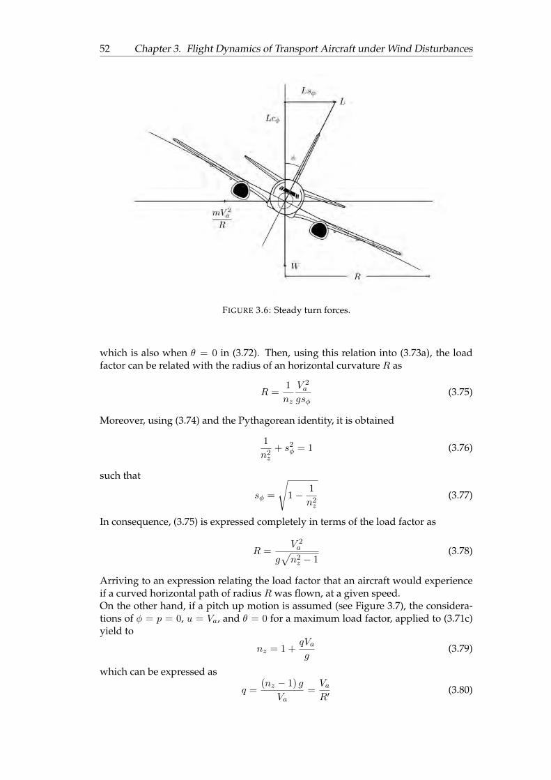
52 Chapter 3. Flight Dynamics of Transport Aircraft under Wind Disturbances
FIGURE 3.6: Steady turn forces.
which is also when θ = 0 in (3.72). Then, using this relation into (3.73a), the loadfactor can be related with the radius of an horizontal curvature R as
R =1
nz
V 2a
gsφ(3.75)
Moreover, using (3.74) and the Pythagorean identity, it is obtained
1
n2z
+ s2φ = 1 (3.76)
such that
sφ =
√1− 1
n2z
(3.77)
In consequence, (3.75) is expressed completely in terms of the load factor as
R =V 2a
g√n2z − 1
(3.78)
Arriving to an expression relating the load factor that an aircraft would experienceif a curved horizontal path of radius R was flown, at a given speed.On the other hand, if a pitch up motion is assumed (see Figure 3.7), the considera-tions of φ = p = 0, u = Va, and θ = 0 for a maximum load factor, applied to (3.71c)yield to
nz = 1 +qVag
(3.79)
which can be expressed as
q =(nz − 1) g
Va=VaR′
(3.80)

3.5. Load factor 53
where R′ is the radius of the vertical curve.As a remark, consider the case of a flight at constant altitude. This can be repre-
FIGURE 3.7: Pitch up motion.
sented as a pitch up motion with an infinite radius R′ =∞. Thus, from (3.80), it canbe said that since Va is a given non-zero value, the expression (nz − 1) g ≈ 0 must betrue. Therefore, since g is the gravity, the only solution is nz = 1, which correspondsto a flight with constant altitude.

54 Chapter 3. Flight Dynamics of Transport Aircraft under Wind Disturbances
3.6 Compilation of equations
3.6.1 Complete Aircraft Dynamics
3.6.1.1 Guidance equations uvw
=
1m (Fxa + Fthr)− gsθ + rv − qw
1mFya + gcθsφ + pw − ru1mFza + gcθcφ + qu− pv
(3.81)
FxaFyaFza
= LBW
−DY−L
(3.82)
DYL
=1
2ρSV 2
a
CDCYCL
(3.83)
VE =
xE˙yE˙zE
= LEB
uvw
(3.84)
VB =
uvw
=
Vacαcβ + VwxVasβ + VwyVasαcβ + Vwz
(3.85)
xEyEzE
= LEB
Fxa + FthrFyaFza
1
m+
00g
(3.86)
3.6.1.2 Attitude equations
pqr
=1
B(AC − E2)
BC 0 BE0 AC − E2 0BE 0 AB
(B − C)qr + Epq + L′
(C −A)pr − E(p2 − r2) +M(A−B)pq − Erq +N
(3.87) L′
MN
=1
2ρSV 2
a
bClcCmbCn
+
bClδail 0 bClδrud0 cCmδele 0
bCnδail 0 bCnδrud
δailδeleδrud
(3.88)
φ
θ
ψ
=
1 tgθsφ tgθcφ0 cφ −sφ0
sφcθ
cφcθ
pqr
(3.89)
α
β
Va
=
H11 H12 H13
H21 H22 H23
H31 H32 H33
pqr
+
Q1
Q2
Q3
(3.90)
3.6.1.3 Actuator equations
δi =1
ξi
(δdi − δi
)(3.91)

3.6. Compilation of equations 55
Fthr =1
ξT
(F dthr − Fthr
)(3.92)
3.6.2 Reduced Aircraft Dynamics
3.6.2.1 Longitudinal motion
γ =1
mVa(L+ Fthrsα −mgcγ)− q
(Vwxcα + Vwzsα
Va
)+
1
Va
(Vwzcα − Vwxsα
)(3.93)
Va =1
m(Fthrcα −D −mgsγ) + q (Vwxsα − Vwzcα)− Vwxcα − Vwzsα (3.94)
xE = Vacγcψ + Vwxcθcψ + Vwzsθcψ (3.95)zE = −Vasγ − Vwxsθ + Vwzcθ (3.96)
θ = q (3.97)
q =M
B(3.98)
3.6.2.2 Lateral motion
β =1
Va
(g (cβsφ − sαsβcφ) +
1
m(Y − Fthrcαsβ)
)+ p
(sα +
Vwzcβ + Vwysαsβ
Va
)+ r
(−cα −
(Vwycαsβ + Vwxcβ)
Va
)+
1
Va
(Vwxcαsβ − Vwycβ + Vwzsαsβ
)(3.99)
yE = Vacγsψ + Vwxcθsψ + Vwycψ + Vwzsθsψ (3.100)
ψ =g
Vatanφ (3.101)
φ = p (3.102)
ψ = rcφ (3.103)
p =1
AC − E2
(CL′ + EN
)(3.104)
r =1
AC − E2
(EL′ +AN
)(3.105)
3.6.3 Load Factor equations
nx = −sθ +(rv − qw)
g(3.106)
ny = cθsφ +(pw − ru)
g(3.107)
nz = cθcφ +(qu− pv)
g(3.108)

56 Chapter 3. Flight Dynamics of Transport Aircraft under Wind Disturbances
3.7 Conclusion
The principal reference frames and their corresponding rotation matrices were pro-vided. They allow a particular representation of a 6DOF aircraft motion using a setof nonlinear differential equations. These equations were rearranged so they fit intothe purposes of this work. A clear example is the wind consideration in the AoA,sideslip and airspeed, instead of a wind disturbance directly in the aircraft position.Furthermore, an introduction to the aerodynamic coefficients of an aircraft was pro-vided. Nevertheless, this topic is complemented in Chapter 4.In addition to this, load factor assumptions for the pitching motion and steady turnshave been considered, such that instead of expressing the load factor of an aircraftdepending on the aircraft state, it was expressed depending on the curvature of thetrajectory that is following. Thus, the obtained expressions could be used for pathgeneration purposes.No aeroelasticity effects were considered, nor the effects of high lift devices or draggenerating elements such as flaps, slats or landing gear.

57
Chapter 4
6DOF Transport AircraftSimulation using MATLAB
After obtaining all the nonlinear differential equations that describe the full be-haviour of a transport aircraft, these are used to develop a six degree of freedomMatlab (Matlab, 2017) model, described in this chapter. The aircraft parameters werechosen similar to an aircraft type Boeing 737-200 or an Airbus 320-200, flying in anInternational Standard Atmosphere model with uniform gravity.One of the main challenges of simulating a full aircraft is in obtaining the aerody-namic nondimensional coefficient values. This is because each coefficient is com-posed by one or more nondimensional stability derivatives, and that they differ fromplane to plane. In general, resources like fluid analysis, wind tunnel tests, or databases are available to obtain these values. However, issues are encountered for eachoption.In this work, the lack of wind tunnels and need of an aircraft mock up, as well assteakholders not sharing easily enough this information, has led to software analy-sis.Hence, data bases were obtained only from public domain softwares, such that any-one is able to reproduce or modify the presented approach. First, the static stability,control and dynamic derivative characteristics of the chosen aircraft are computedusing the methods contained in the USAF Stability and Control DATCOM. Then,the obtained data is compared and refined using the corresponding JSBSim opensource Flight Dynamic Model (FDM). JSBSim is employed to drive the motion-baseresearch simulators of many universities worldwide.Furthermore, due to the complexity and size of the data bases, two-layer feed-forwardneural networks with sigmoid hidden neurons and linear output neurons were trainedto obtain the values of the coefficients: CD,Y,L, Clβ,p,r,δail,δrud ;Cm0,α,q,δele
;Cnβ,p,r,δail,δrud ,allowing to develop a complete aircraft model.As a result, Section 4.1 of this chapter is subdivided in three subsections. Subsections4.1.1 and 4.1.2 are an extensive background on machine learning towards supervisedlearning, in order to better understand the neural networks used in the simulation.Subsection 4.1.3, regards to relevant information about the stability derivatives aswell as their numerical values for our case study.Section 4.2 shows the aircraft behaviour in open loop, so that the model is verifiedaccording to the theory presented.Finally, conclusions are given in Section 4.4.
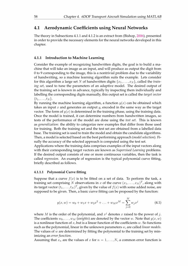
58 Chapter 4. 6DOF Transport Aircraft Simulation using MATLAB
4.1 Aerodynamic Coefficients using Neural Networks
The theory in Subsections 4.1.1 and 4.1.2 is an extract from (Bishop, 2006), presentedin order to provide the necessary elements for the neural networks developed in thischapter.
4.1.1 Introduction to Machine Learning
Consider the example of recognizing handwritten digits, the goal is to build a ma-chine that will take an image as an input, and will produce as output the digit from0 to 9 corresponding to the image, this is a nontrivial problem due to the variabilityof handwriting, so a machine learning algorithm suits the example. Lets considerfor this algorithm a large set N of handwritten digits x1, . . . , xN, called the train-ing set, used to tune the parameters of an adaptive model. The desired output ofthe training set is known in advance, typically by inspecting them individually andlabelling the corresponding digits manually, this output set is called the target vectort1, . . . , tN.By running the machine learning algorithm, a function y(x) can be obtained whichtakes an input x and generates an output y, encoded in the same way as the targetvector. The form of y(x) is determined in the training phase, using the training data.Once the model is trained, it can determine numbers from handwritten images, sotests of the performance of the model are done using the test set. This is knownas generalization: the ability to categorize new examples that differ from those usedfor training. Both the training set and the test set are obtained from a labelled database. The training set is used to train the model and obtain the candidate algorithms.Then, a model is selected based on the best performing approach (model selection). Fi-nally the accuracy of the selected approach is computed using the test set.Applications where the training data comprises examples of the input vectors alongwith their corresponding target vectors are known as Supervised Learning problems.If the desired output consists of one or more continuous variables, then the task iscalled regression. An example of regression is the typical polynomial curve fitting,briefly described as follows.
4.1.1.1 Polynomial Curve fitting
Suppose that a curve f(x) is to be fitted on a set of data. To perform the task, atraining set comprising N observations in x of the curve (x1, . . . , xN )T , along withits target vector (t1, . . . , tN )T , given by the value of f(x) with some added noise, aresupposed to be given. Then, a basic curve fitting can be proposed by the function:
y(x,w) = w0 + w1x+ w2x2 + . . .+ wMx
M =M∑j=0
wjxj (4.1)
where M is the order of the polynomial, and xj denotes x raised to the power of j.The coefficients w0, . . . , wM (weights) are denoted by the vector w. Note that y(x,w)is a nonlinear function of x, but is a linear function of the coefficients w. So functionssuch as the polynomial, linear in the unknown parameters w, are called linear models.The values of w are determined by fitting the polynomial to the training set by min-imizing an error function.Assuming that xn are the values of x for n = 1, . . . , N , a common error function is

4.1. Aerodynamic Coefficients using Neural Networks 59
given by the sum of the squares of the error between the predictions y(xn, w) foreach data point xn and the corresponding target values tn:
E(w) =1
2
N∑n=1
y(xn, w)− tn2 (4.2)
The curve fitting problem can be solved by choosing values for w, such that E(w)is as small as possible. Since the error function is a quadratic function of the coef-ficients w, its derivatives with respect the coefficients will be linear in the elementsof w, and so the minimization of the error function has a unique solution w∗, whichcan be found in closed form. The resulting polynomial will be given by y(x,w∗).Then, the remaining problem is to choose the order M of the polynomial, in otherwords, the model selection. Some problems of the model selection are a poor rep-resentation of the curve to be fitted, and the over-fitting phenomenon, which willhappen if E(w∗) = 0, but the polynomial does not fit properly the curve proposed.Since the goal is to make a good generalization by making accurate predictions fornew data, a good model selection can be made by evaluating for each choice of M ,the residual value of E(w∗) (given by (4.2)) for the training data. Moreover, E(w∗)can be evaluated for the test set to measure how well the model is predicting the val-ues of t for new data observations of x. It is convenient to use the root-mean-squareerror, measured in the same scale and units as the target variable t, defined by:
ERMS =√
2E(w∗)/N (4.3)
As the size of N increases, the more complex model can be used to fit to the data.In addition to this, it will be seen that the use of least squares to find the model pa-rameters represents a specific case of maximum likelihood, and the over-fitting prob-lem can be understood as a general property of maximum likelihood. Therefore, inorder to avoid the over-fitting problem, a Bayesian approach can be adopted.Another technique often used to control the over-fitting problem is the regularization,which involves adding a penalty term to the error function (4.2) in order to discour-age the coefficients from reaching large values. The simplest expression of the newerror function under this idea is expressed by:
E(w) =1
2
N∑n=1
y(xn, w)− tn2 +λ
2‖w‖2 (4.4)
where ‖w‖2 = wTw = w20 + w2
1 . . . + w2M , and the coefficient λ handles the relative
importance of the regularization term compared with the sum-of-squares error term.The particular case of a quadratic regularizer is called ridge regression. Besides, aneffect of the regularization is to reduce the magnitude of the coefficients w.In gerneral, the training set will be used to determine the coefficients w, and thevalidation set will be used to optimize the model complexity (M , λ).
4.1.1.2 Bayesian Approach
Imagine two boxes, one red, one blue, with the red box containing 2 apples and 6oranges, and the blue containing 3 apples and 1 orange. Suppose that one of theboxes is picked randomly, and one fruit is selected from the box. Then, after seeingthe sort of fruit that was picked, it is put back in the box. Assume that the redbox is picked the 40% of time and the blue the other 60%. By denoting the random

60 Chapter 4. 6DOF Transport Aircraft Simulation using MATLAB
variables B for box, F for fruit, and the values of r = red, b = blue, a = apple, ando = orange, the probability of selecting the red box is expressed as p(B = r) = 4/10and p(B = b) = 6/10. Note that all probabilities must lie in the interval [0, 1], andthat the probability of an event is defined as the fraction of times that the eventoccurs out of the total number of trials, in the limit that the total number of trialstends to infinity. Note also that p(B = r) + p(B = b) = 1.In the same way, it is known that the probability of selecting an apple from the bluebox is 3/4, so the conditional probabilities, starting with the latter mentioned are:
• p(F = a|B = b) = 3/4
• p(F = a|B = r) = 1/4
• p(F = o|B = b) = 1/4
• p(F = o|B = r) = 3/4
Again, lets note that
p(F = a|B = r) + p(F = o|B = r) = p(F = a|B = b) + p(F = o|B = b) = 1 (4.5)
and using the rules of sum and product of probability, the overall probability ofchoosing an apple can be evaluated by:
p(F = a) = p(F = a|B = r)p(B = r) + p(F = a|B = b)p(B = b)
=1
4× 4
10+
3
4× 6
10=
11
20(4.6)
so, p(F = o) = 1− 11/20 = 9/20.Now, lets assume that a fruit has been selected and it is an orange, and it is desiredto know from which box it came from, one can solve the problem of reversing theconditional probability by using the Bayes theorem. This yields:
p(B = r|F = o) =p(F = o|B = r)p(B = r)
p(F = o)
=3
4× 4
10× 20
9=
2
3(4.7)
so, p(B = b|F = o) = 1− 2/3 = 1/3.An important interpretation of the Bayes theorem can be provided. If it would havebeen asked which box had been chosen before being told the selected fruit, then themost complete information available is provided by the probability p(B). This iscalled the prior probability, because it is the probability available before the obser-vation of the identity of the fruit. Once it is known that the fruit is an orange, theBayes theorem can be used to compute the probability p(B|F ), which will be calledthe posterior probability, because is the probability obtained after the observation ofF . Note that the prior probability of selecting the red box was 4/10, so it is morelikely to select the blue box. However, once it was observed that the selected fruitis an orange, the posterior probability of the red box is now 2/3, so that it is nowmore likely that the box selected was in fact the red one. Corroborating that the ob-servation that the fruit was an orange, provides significant evidence favouring thered box. Moreover, this evidence is strong enough to outweigh the prior probabilityof selecting the blue box.Now, after pointing out the advantages of a Bayesian approach, where probabilities

4.1. Aerodynamic Coefficients using Neural Networks 61
provide a quantification of uncertainty rather than the typical frequentist interpreta-tion of probability based on frequencies of random, repeatable events, let us recon-sider the polynomial curve fitting example.In the polynomial fitting, assumptions about the parameters w can be made beforeobserving the data, in the form of a prior probability distribution p(w). Then, theeffect of the observed data D = t1, . . . , tN is expressed through the conditionalprobability p(D|w), and it will be shown how this can be represented explicitly.Hence, the Bayes theorem takes the form of
p(w|D) =p(D|w)p(w)
p(D)(4.8)
which allows the evaluation of the uncertainty in w after the observation of D in theform of the posterior probability p(w|D).The quantity p(D|w) of (4.8) is evaluated for the observed data set D and can beviewed as a function of the parameter vectorw, in which case it is called the likelihoodfunction. It expresses how probable the observed data set is for different settings ofthe parameter vector w. Note that the likelihood is not a probability distributionover w. Hence, its integral with respect to w does not (necessarily) equal to one. Inother words, the Bayes theorem can be expressed as:
posterior ∝ likelihood× prior
where all these are viewed as functions of w. The term p(D) in (4.8) is the nor-malization constant, which ensures that the left hand-side of the equation is a validprobability density and integrates to one.In both Bayesian and frequentist paradigms, the likelihood function p(D|w) is fun-damental but is used differently depending on the approach. For the frequentistsetting, w is considered to be a fixed parameter, which is determined by some "esti-mator", and error bars on this estimate are obtained by considering the distributionof possible data setsD. On the other hand, for the Bayesian approach, there is only asingle data set D, which is the one observed, and the uncertainty in the parametersis expressed through a probability distribution over w.In the maximum likelihood frequentist estimator, w is set to the value that maximizesthe likelihood function. This corresponds to choosing w such that the probability ofthe observed data set is maximized.In the machine learning literature, the monotonically decreasing function given bythe negative log of the likelihood function is the error function, because maximizingthe likelihood is equivalent to minimizing the error.The advantage of the Bayesian approach can be seen in the inclusion of prior knowl-edge. Suppose for example that a coin is flipped three times, and every time it landsheads. The classical maximum likelihood estimate of the probability of landingsheads would be 1, implying that all future tosses will be heads. In contrast, theBayesian approach with reasonable prior information will lead to a less extreme con-clusion.Therefore, in the curve fitting problem viewed from a probabilistic perspective, thegoal is to make predictions for the target variable t given a new value of the scalarinput variable x, using a training set comprising N input observation values X =(x1, . . . , xN )T and their corresponding target values T = (t1, . . . , tN )T . In this man-ner, the uncertainty over the value of the target variable can be expressed using aprobability distribution. For this purpose, it is assumed that, given the value of x,
62 Chapter 4. 6DOF Transport Aircraft Simulation using MATLAB
the corresponding value of t has a Gaussian distribution1 with a mean equal to thevalue y(x,w) of the polynomial curve given by (4.1). Thus:
p(t|x,w, β) = N (t|y(x,w), β−1) (4.9)
where β corresponds to the inverse variance of the Gaussian distribution.Now, the values of the unknown parametersw and β are determined using the train-ing data X,T via maximum likelihood. If the training data is assumed to be takenindependently from the distribution (4.9), then the likelihood function is given by
p(T|X, w, β) =
N∏n=1
N (tn|y(xn, w), β−1) (4.10)
As shown in the Appendix B.2, where the maximum likelihood approach is usedto perform a regression of a Gaussian distribution, it is convenient to maximize thelogarithm of the likelihood function. In this manner, using (B.1), which describesmathematically the Gaussian distribution, it is obtained
lnp(T|X, w, β) = −β2
N∑n=1
y(xn, w)− tn2 +N
2lnβ − N
2ln(2π) (4.11)
The first maximum likelihood solution for the polynomial coefficients will be de-noted by wML, obtained by maximizing (4.11) with respect to w. Some interestingresults are derived from this. Note that the last 2 terms of the right-hand side canbe omitted, as they do not depend on w. Then, scaling the log likelihood by a posi-tive constant coefficient β, does not alter the location of the maximum with respectto w. Consequently, β/2 can be replaced by 1/2. Finally, instead of maximizing thelog likelihood, is equivalent to minimize the negative log likelihood. Therefore, it isclearly seen that maximizing the likelihood to obtain the parameters w is the sameas minimizing the sum-of-squares error function, defined previously in (4.2). Thus thesum-of-squares error function is a consequence of maximizing the likelihood underthe assumption of a Gaussian noise distribution.Also, maximizing (4.11) with respect to the precision parameter β of the Gaussianconditional distribution yields
1
βML=
1
N
N∑n=1
y(xn, wML)− tn2 (4.12)
Now that the parameters w and β have been determined, predictions for new val-ues of x can be made. Since a probabilistic model is obtained, the predictions areexpressed by a predictive distribution that gives the probability distribution over trather than simply a point estimate. Hence (4.9) turns into
p(t|x,wML, βML) = N (t|y(x,wML), β−1ML) (4.13)
Therefore, in order to advance towards a Bayesian approach, it is introduced a Gaus-sian prior distribution over the polynomial coefficients w, given by
p(w|α) = N (w|0, α−1I) =( α
2π
)(M+1)/2exp
−α
2wTw
(4.14)
1For more information on Gaussian distribution, refer to Appendix B.1

4.1. Aerodynamic Coefficients using Neural Networks 63
where α is the precision of the distribution, andM+1 is the total number of elementsin the vector w for an M th order polynomial. Variables such as α, which control thedistribution of model parameters, are called hyperparameters. Then, using the Bayestheorem, the posterior distribution for w is proportional to the product of the priordistribution and the likelihood function, denoted by
p(w|X,T, α, β) ∝ p(T|X, w, β)p(w|α) (4.15)
In this manner, w can be determined by finding the most probable value of w giventhe data. This, therefore, involves maximizing the posterior distribution, and usingthe technique is called maximum posterior. Taking the negative logarithm of (4.15)and using (4.11) and (4.14), the maximum of the posterior is given by the minimumof
β
2
N∑n=1
y(xn, w)− tn2 +α
2wTw (4.16)
At this point, it is clear that maximizing the posterior distribution is equivalent tominimizing the regularized sum-of-squares error function encountered in (4.4), witha regularization parameter denoted by λ = α/β
4.1.1.3 Bayesian curve fitting
Knowing the training data X and T, along with a new test point x, the goal is topredict the value of t. Therefore, the predictive distribution p(t|x,X,T) needs to beevaluated. It is assumed that the parameters α and β are known in advance. Thus,the predictive distribution can be written as
p(t|x,X,T) =
∫p(t|x,w)p(w|X,T)dw (4.17)
where p(t|x,w) is given by (4.9), omitting the dependence on α and β to reduce nota-tion. Here p(w|X,T) is the posterior distribution over parameters, and can be foundby normalizing the right-hand side of (4.15). This posterior distribution will turn outto be a Gaussian and can be evaluated analytically. Similarly, the integration in (4.17)can also be performed analytically with the result that the predictive distribution isgiven by a Gaussian of the form
p(t|x,X,T) = N (t|µ(x), σ2(x)) (4.18)
where the mean (µ) and variance (σ2) are given by
µ(x) = βφ(x)TSN∑n=1
φ(xn)tn (4.19)
σ2(x) = β−1 + φ(x)TSφ(x) (4.20)
and the matrix S is expressed by
S−1 = αI + βN∑n=1
φ(xn)φ(x)T (4.21)
where I is the unit matrix, and the vector φ(x) is defined with the elements φi(x) = xi
for i = 0, . . . ,M . The mean and the variance of the predictive distribution in (4.18)

64 Chapter 4. 6DOF Transport Aircraft Simulation using MATLAB
are dependent on x.In this manner, the first term in (4.20) represents the uncertainty in the predictedvalue of t due to the noise of the target variables and was expressed in the maximumlikelihood predictive distribution (4.13) through β−1. However, the second termcomes from the uncertainty in the parametersw and is a consequence of the Bayesiantreatment.
4.1.1.4 Model Selection
In the polynomial curve fitting example using least squares, the optimal order of thepolynomial is the one that gives the best generalization, and the order (M ) of thepolynomial controls the number of free parameters (w) in the model, and therefore,the model complexity. In the case of regularized least squares, the regularization co-efficient (λ) also controls the complexity of the model, and for more complex models,there may be multiple parameters governing complexity. In a practical application,the values of these coefficients must be determined such that the best prediction per-formance on new data is achieved.It has been seen in the maximum likelihood approach that the performance on thetraining set is not a good indicator of predictive performance on unseen data dueto the over-fitting problem. So one approach is to use some of the available data totrain a range of models, or a given model with a range of values for its complexityparameters. Then, the models are compared using independent data, called a vali-dation set, and finally the model with the best predictive performance is selected.If the validation set is too small, it will give a relatively noisy estimate of predictiveperformance, so one solution to this is cross validation. The cross validation tech-nique consists in dividing the available data in S groups and taking S − 1 groupsto train a set of models that are evaluated in the remaining group. This is repeatedfor all S possible choices, and then the scores from the S runs are averaged. Thedisadvantage of this approach is that the computational complexity is increased asthe number of training runs is increased by a factor S, and exponentially increasedif several parameters are tested in different combinations.
4.1.1.5 Linear Models for Regression
Consider that the goal of regression is to predict the value of one or more targetvariables t given the value of a D−dimensional vector x of input variables. Givena training data set comprising N observations xn, where n = 1, . . . , N , togetherwith their correspondent target values tn, the goal is to predict the value of t for anew value of x. Note that x = (x1, . . . , xD)T .The simplest linear model for regression is a linear combination of the input vari-ables:
y(x, w) = w0 + w1x1 + . . .+ wDxD (4.22)
This is known as linear regression, with a linear function of the parametersw0, . . . , wDand a linear function of the inputs variables x1, . . . , xD. However, much more usefulclass of functions can be obtained by taking linear combinations of a fixed set ofnonlinear functions of the input variables, known as basis functions. Hence:
y(x, w) = w0 +M−1∑j=1
wjφj(x) (4.23)

4.1. Aerodynamic Coefficients using Neural Networks 65
where φj(x) are the basis functions. By denoting the maximum value of the index jby M − 1, the total number of parameters will be M .The parameter w0, called bias, allows to introduce a fixed offset in the data. It isuseful to define an additional basis function φ0(x) = 1 so that
y(x, w) =M−1∑j=0
wjφj(x) = wTφ(x) (4.24)
where w = (w0, . . . , wM−1)T and φ = (φ0, . . . , φM−1)T .By using nonlinear basis functions, y(x, w) is allowed to be a nonlinear function ofthe input vector x.An example of a linear model is the polynomial regression for fitting a curve, whereinstead of having an input vector x, a single input variable x is needed, so the basisfunctions take the form φj(x) = xj .There are many other possible choices for the basis functions, for example
φj(x) = exp
−(x− µj)2
2s2
(4.25)
where µj governs the locations of the basis functions in input space, and the parame-ter s governs their spatial scale. This is known as a Gaussian basis function. Anotherpossibility is the sigmoidal basis function:
φj(x) = σ
(x− µjs
)(4.26)
whereσ(a) =
1
1 + exp(−a)(4.27)
Equivalently, the hyperbolic tangent (tanh) function can be used, knowing that
tanh(a) = 2σ(a)− 1 (4.28)
Another possible choice of basis functions is the Fourier basis, which leads to anexpansion in sinusoidal functions. Also, a class of functions known as wavelets aremore applicable for signal processing problems.
4.1.2 Neural Networks Model
So far, models for regressions comprising linear combinations of fixed basis func-tions have been considered. However, as they are limited by dimensionality, thebasis functions can be adapted to the data. One approach to do this is to fix thenumber of basis functions in advance but allowing them to be adaptive. In otherwords, to use parametric forms for the basis functions in which the parameters val-ues are adapted during training. The most successful model of this is the feed-forwardneural network, also known as the multilayer perceptron, which gives a compact, fastmodel, with high generalization performance.The linear models for regression are based on linear combinations of fixed nonlinear

66 Chapter 4. 6DOF Transport Aircraft Simulation using MATLAB
basis functions φj(x) with the form
y(x, w) = f
M∑j=1
wjφj(x)
(4.29)
where f(·) is a nonlinear activation function equal to the identity in the case of re-gression. Neural networks (NNs) use basis functions that follow the same form as(4.29). Therefore, each basis function is itself a nonlinear function of a linear com-bination of the inputs, where the coefficients in the linear combination are adaptiveparameters.Then, it is time to provide the basic neural network model.First, M linear combinations of the input variables x1, . . . , xD are constructed in theform
aj =
D∑i=1
w(1)ji xi + w
(1)j0 (4.30)
where j = 1, . . . ,M , and the superscript (1) indicates that the corresponding pa-rameters are in the first layer of the network. From now on, w(1)
ji are referred to as
weights, and the parameters w(1)j0 as biases. The quantities aj are known as activations.
Each of them is transformed using a differentiable nonlinear activation function h(·)to give
zj = h(aj) (4.31)
These quantities correspond to the outputs of the basis functions in (4.29), referredto as hidden units. The typical choice for the nonlinear functions h(·) are sigmoidalfunctions. Thus, following (4.29), these values are again linearly combined to giveoutput unit activations
ak =
M∑j=1
w(2)kj zj + w
(2)k0 (4.32)
where k = 1, . . . ,K, and K is the total number of outputs. This transformationcorresponds to the second layer of the network. Finally, the output unit activationsare transformed using an appropriate activation function to give a set of networkoutputs yk. The activation function is the identity in regression problems, such that
yk = ak (4.33)
Combining the stages, the overall network function for a regression problem takesthe form
yk(x,w) =
M∑j=1
w(2)kj h
(D∑i=1
w(1)ji xi + w
(1)j0
)+ w
(2)k0 (4.34)
where the set of all weight and bias parameters have been grouped together into avector w. Thus, the neural network model is a nonlinear function from a set of inputvariables xi to a set of output variables yk, controlled by a vector w of adjustableparameters. The neural network architecture is shown in Figure 4.1.
This network, being the most commonly used in practice, may be described as a2-layer feed-forward neural network, because it is the number of layers of adaptiveweights. A two-layer network with linear outputs can uniformly approximate anycontinuous function on a compact input domain.

4.1. Aerodynamic Coefficients using Neural Networks 67
FIGURE 4.1: Neural Network architecture.
Determining the neural network parameters within a maximum likelihood frame-work involves the solution of a nonlinear optimization problem. This requires theevaluation of derivatives of the log likelihood function with respect to the networkparameters, obtained efficiently using the error back propagation technique. This train-ing technique is not covered in this manuscript.
4.1.3 Aerodynamic Coefficients
According to (Stevens and Lewis, 1992), the various dimensionless aerodynamic co-efficients are primarily dependent on the AoA and sideslip angle, and less depen-dent on other variables. Nevertheless, the dependence of the coefficients on angularvelocities is taken into account for this work since they play an important role in theaircraft motion. The relations describing the aerodynamics coefficients were givenin the previous chapter as CL
CYCD
=
CLααCYββ
CD(CL)
ClCmCn
=
Clββ + Clpbp
2Va+ Clr
br2Va
Cm0 + Cmαα+ Cmqcq
2Va
Cnββ + Cnpbp
2Va+ Cnr
br2Va
where each one of the nondimensional coefficients is composed by one or morenondimensional stability derivatives.Furthermore, the contributions of the control surfaces moments is included in (3.21),which is
Mext =
L′
MN
=1
2ρSV 2
a
bClcCmbCn
+
bClδail 0 bClδrud0 cCmδele 0
bCnδail 0 bCnδrud
δailδeleδrud

68 Chapter 4. 6DOF Transport Aircraft Simulation using MATLAB
The numerical values of these nondimensional stability derivatives change fromplane to plane, and the means to obtain these values are computation of fluid dy-namics, wind tunnel tests, or data bases gathering this information. When numeri-cal simulations are carried out, it is a common practice to assume the values of thesederivatives as constants, loosing accuracy but gaining simplicity in the simulation.In this work, a group of neural networks, one for each nondimensional stabilityderivative is proposed.From now on, the nondimensional stability derivatives will be referred to just as thestability derivatives.At this point, the reader may wonder why the use of Neural Networks is preferredinstead of N-dimensional lookup tables with interpolation between values. The an-swer is quite simple, a Neural Networks approach provides a significant simplicitywhen multi-input / multi-output data is handled. Also, the possibility of onlineimprovement of the neural networks with new airborne information in case of ab-normal situations (icing, disfigurations in profile, major inertial matrix changes, etc.)is of great interest.Thus, as neural networks need a data base to be trained, it is imperative to obtain adata base of the aerodynamic coefficients or the stability derivatives. Unfortunately,since access to experimental data bases of this coefficients is almost impossible dueto enterprises privacy policies, and the use of wind tunnels to measure this coeffi-cients is also unfeasible, the only resource left is software simulation.Consequently, data bases were obtained from the United States Air Force (USAF)Stability and Control Digital DATCOM (Data Compendium) (Williams and Vuke-lich, April 1979). This Public Domain Aeronautical Software computes the staticstability, control and dynamic derivative characteristics of fixed-wing aircrafts usingthe methods contained in the USAF Stability and Control DATCOM. Furthermore,the data sets were compared and refined using the JSBSim open source Flight Dy-namics Models (FDM) (JSBsim, 2016), used in several open source simulators andalso employed to drive the motion-base research simulators of many universitiesworldwide.The first step in the coefficient obtention is to draw the aircraft using built-in com-mands provided in the DATCOM software, which resulted in Figure 4.2 (dimensionsare in feet). Then, the aircraft geometry in the form of a script is processed by theprogram and the aerodynamic data is provided in tables.After the datasets are obtained for each stability derivative, the training, validation
and test sets are defined to be the 70, 15 and 15 percent, respectively, of the availabledata. The training algorithm used is the Bayesian Regularization and the number ofhidden neurons is selected by trial and error trying to improve the performance asmuch as possible.All simulations performed here are at subsonic speeds, and the stability derivativesare computed per-radian.Furthermore, the performance of the neural networks developed to fit the availabledata is given in Appendix C, using the Mean Squared Error of the training and test-ing data sets.The reader must have in mind that all the stability derivatives are the result of approximatedmodels and neural networks with limited datasets.This model was created using publicly available data, publicly available technical reports,textbooks, and estimates. It contains no proprietary or restricted data. If this model has beenvalidated at all, it would be only to the extent that it seems to "fly right", and that it possiblycomplies with published, publicly known, performance data. Thus, this model is meant foreducational and entertainment purposes only.

4.1. Aerodynamic Coefficients using Neural Networks 69
FIGURE 4.2: Aircraft drawing (Dimensions in feet).
This simulation model is not endorsed by the manufacturer. This model is not to be sold.
4.1.3.1 Lift and Drag Coefficients
Regarding the Lift coefficient, a dependence on the AoA is shown in Figure 4.3,where it can be seen how as the AoA increases, so does the Lift coefficient. Thus,if the stability derivative CLα was obtained, it would have a positive value. Notethat high Lift devices such as flaps or slats are not considered. Thus, for take-off andlanding, the coefficient would have to be modified with the corresponding effects.Once that the Lift coefficient is known, the Drag coefficient can be obtained from it,this is done using a parabolic equation of the form
CD = CD0 + CDiC2L (4.35)
where CD0 = .0176 is the parasitic drag coefficient, and CDi = .0515 is the induceddrag coefficient. Note that this equation is only valid for nominal conditions. Forlanding or approaching, where flaps or the landing gear have drag contributions,other coefficients should be considered.The resultant Drag coefficient is plot in Figure 4.4. Note that the Drag coefficientincreases as the AoA increases. Therefore, a derivative CDα would be also positive.
4.1.3.2 Sideforce Coefficient
Regarding the lateral force CY , the main contribution is supposed to be given by thesideslip angle, such that the nondimensional stability derivativeCYβ is its main com-ponent. The variation of this derivative with respect to the airspeed and the angle ofattack is provided in Figure 4.5.
Since CYβ has a negative value, and the coefficient CY is given by the product ofCYββ, this means that a positive sideslip angle (sideslip to the right), will generate anegative lateral force (force to the left). This force is due to the drag of the aircraftvertical surfaces such as the fuselage or vertical fin.Moreover, a lateral force due to the rudder deflection could be taken into account,

70 Chapter 4. 6DOF Transport Aircraft Simulation using MATLAB
FIGURE 4.3: Coefficient CL.
FIGURE 4.4: Coefficient CD.

4.1. Aerodynamic Coefficients using Neural Networks 71
FIGURE 4.5: Coefficient CYβ .
but as its influence is weaker than the one of the sideslip angle, this force is neglected.
4.1.3.3 Rolling moment
Figure 4.6 is provided to follow this subsection easily.To begin, the rolling coefficient is considered to be given by
FIGURE 4.6: Top and front view of a plane showing a positive β. Theright and left wings are in low positions and are denoted by R, L,respectively. Positive sweep angle of the wings along with a positive
wing dihedral is also shown.
Cl = Clββ + Clpbp
2Va+ Clr
br
2Va

72 Chapter 4. 6DOF Transport Aircraft Simulation using MATLAB
where the first contribution, Clβ , is the combination of four influences:
• The wing dihedral effect:For a positive sideslip in an aircraft with positive wing dihedral (upward), theAoA of the right wing is increased, and the AoA of the left wing is decreased.Therefore, the lift of the right wing is more than the one on the left wing, cre-ating a negative rolling moment (to the left).
• The wing sweep angle:For a positive sideslip in an aircraft with positive sweep of the wings (sweep-back), the speed of the right wing is lightly increased with respect to the leftwing, provoking more lift on the right wing compared to the left wing. Thiscreates a negative rolling moment (to the left).
• The wing position (high/low):In this component, the high position refers to wings above the fuselage, andlow to wings situated below the fuselage.For a positive sideslip in the high wing position, the pressure increase on theright wing lower surface, creating more lift in this side of the wing. Conse-quently, a negative rolling moment is created.For a positive sideslip in the low wing position, the pressure increase on theright wing upper surface, creating less lift in this side of the wing. Conse-quently, a positive rolling moment is created.
• The vertical tail:Since the vertical tail’s centre of pressure is typically above the CxB axis, apositive sideslip will generate a drag force due to the vertical tail drag actuat-ing in the upper part of the rotation axis, creating a negative rolling moment.Hence, the placement of vertical fins below the CxB axis will counteract thiscomponent with a positive rolling moment.
Since the wing dihedral effect is the most significant, sometimes this nondimen-sional stability derivative is called the dihedral effect. Thus, the general behaviour ofthe aircraft is a negative rolling motion at positive sideslip angles (yielding a nega-tive value of the derivative).Note 1: 1 of dihedral angle has the same effect as 6 of sweep angle.Note 2: The horizontal stabilizer also contributes to this derivative; it can featuredihedral, sweep and high/low position.The variation of this derivative with respect to the airspeed and the angle of attackis provided in Figure 4.7.
The second component of the rolling moment is the one induced by a roll rate,given by the derivative Clp . Considering an initial positive roll rate, additional ve-locity components affect the wings. The right wing is dropping and increasing itsAoA, and the left wing is rising and decreasing its AoA. This generates more lift inthe right wing than in the left one, creating a negative rolling moment counteract-ing the initial motion. Thus, this component of the rolling moment can be seen as adamping, helping to the static stability of the aircraft. Therefore, the derivative willhave a negative value.The variation of this derivative with respect to the airspeed and the AoA is providedin Figure 4.8.
The third component of the rolling moment is the one induced by the yaw rate,involving the derivative Clr . Considering an initial positive yaw rate, the velocityon the right wing is decreased and in the left wing is increased, generating more lift

4.1. Aerodynamic Coefficients using Neural Networks 73
FIGURE 4.7: Coefficient Clβ .
FIGURE 4.8: Coefficient Clp .

74 Chapter 4. 6DOF Transport Aircraft Simulation using MATLAB
in the left wing compared to the right wing, provoking a positive rolling moment.In this manner, this derivative with positive value, acts in the opposite sense as theone produced by the roll rate, not helping to the static stability.The variation of this derivative with respect to the airspeed and the AoA is providedin Figure 4.9.Regarding the moments generated by the control surfaces, the first to be considered
FIGURE 4.9: Coefficient Clr .
is the rolling moment provoked by the ailerons deflection. When the right aileron islowered and the left aileron is raised, denoted by a positive δail, the lift is spoiled inthe left wing and the lift is increased on the right wing, making the airplane turn tothe left due to a negative rolling moment. Thus, the value of the derivative express-ing this effect is negative. In our simulation, this is a constant value of Clδail = −.02.On the other hand, the moment generated by the rudder deflection involves thederivative Clδrud . Considering a deflection of the rudder to the left, denoted by apositive δrud (clockwise from a top-view of the aircraft with the nose in the upperpart), it will create an added drag component above the CxB axis. Hence, since thisdrag force will act in the upper part of the rotation axis, it will generate a positiverolling moment, named adverse roll, and a negative yawing motion. In consequence,the value of Clδrud should be positive. This adverse effect is weak, and a value ofzero is defined for this derivative in the simulation such that the moment producedis neglected.

4.1. Aerodynamic Coefficients using Neural Networks 75
4.1.3.4 Yawing Coefficient
The yawing coefficient is considered to be given by
Cn = Cnββ + Cnpbp
2Va+ Cnr
br
2Va
where the first contribution Cnβ is also called the weathercock effect, and is the contri-bution of four influences
• The vertical tail and fins:Considering a positive sideslip angle (to the right), the vertical tail experiencesa change in its "AoA". Thus, a sideforce appears on the tail (towards the left),provoking a positive yawing moment (to the right). An interesting remark isthat if the sideslip angle is too big, the vertical tail may stall.
• The wing sweep angle:As seen in the rolling moment created by the dihedral effect, a sweepback an-gle of the wings and a positive sideslip angle, will create an increase in thespeed of the right wing compared to the left, provoking more lift on the rightwing and consequently, more drag. Thus, since more drag is produced in theright wing with respect to the left wing, a positive yawing moment is gener-ated.
• The fuselage:Considering a positive sideslip angle, a side force appears on the fuselage,provoking a positive yawing moment dependent on the center of pressure po-sition.
• The c.g. position:All forces applied in front of the aircraft’s c.g. will generate a negative yawingmoment when a positive sideslip angle is considered.
In general, the contribution of the weathercock effect, is such that for positive sideslipangles, positive yawing moments are generated, causing a positive static stability.Thus, the derivative has a positive value.The variation of this derivative with respect to the angle of attack is provided in Fig-ure 4.10.The second contribution term is the one involving the derivative Cnp . Considering
an initial roll in the positive sense, the left wing will be rising, decreasing its AoA.On the other hand, the right wing will be dropping and increasing its AoA, provok-ing more Drag in the right wing than the left. This means that a positive roll rate,creates a positive yawing motion, called induced yaw. Thus, the derivative has a pos-itive value. The effect of this induced yaw is weak.The variation of this derivative with respect to the AoA and airspeed is provided inFigure 4.11.The third contribution term is the one induced by the yaw rate Cnr . Considering an
initial rate of yaw to the right, the right wing decreases its speed, and consequentlydecreases its drag with respect to the left wing. On the other hand, the left wing in-creases its speed and drag. All combined provokes a negative yawing motion. Thiscomponent of the yawing moment can be seen as a damping, helping to the dynamicstability of the aircraft. Therefore, the derivative will have a negative value.The variation of this derivative with respect to the AoA and airspeed is provided inFigure 4.12.

76 Chapter 4. 6DOF Transport Aircraft Simulation using MATLAB
FIGURE 4.10: Coefficient Cnβ .
FIGURE 4.11: Coefficient Cnp .

4.1. Aerodynamic Coefficients using Neural Networks 77
FIGURE 4.12: Coefficient Cnr .
Regarding the moments generated by the control surfaces, the first to be consideredis the yawing moment provoked by the ailerons deflection. When the right aileronis lowered and the left aileron is raised (positive δail), the raised aileron actuates asa camber decrease which decreases the drag force, and the dropped aileron acts as acamber increase, increasing the drag. Thus, banking to the left provokes a positiveyawing motion, called adverse yaw. The value of the derivative expressing this effectis positive. In our simulation, this is a constant value of Cnδail = .002.On the other hand, the moment generated by the rudder deflection involves thederivative Cnδrud . Considering a deflection of the rudder to the left, denoted by apositive δrud, it will create a strong moment to the left, since it is the very function ofthe rudder. Thus, the value of the derivative is negative. In our simulation, this is aconstant value of Cnδrud = −.07.
4.1.3.5 Pitching Coefficient
The pitching coefficient is considered to be given by
Cm = Cm0 + Cmαα+ Cmqcq
2Va
Before continue with each term of the pitching coefficient, three important consider-ations are pointed out:
• When c.g. is ahead a.c.: Positive static stability.
• When c.g. is behind a.c.: Negative static stability (Instability).

78 Chapter 4. 6DOF Transport Aircraft Simulation using MATLAB
• When c.g. is at a.c.: Neutral static stability.
The location of the c.g. moving backwards is limited by the a.c. position for stabilityreasons. Also, the more forward the c.g. position, the larger the elevator deflectionis needed to pitch the aircraft. In this manner, a forward c.g. position limit is defineddue to controllability reasons. Moreover, one should consider that at larger elevatordeflection, larger drag is generated, leading to more fuel consumption.The first term of the pitching coefficient corresponds to the intrinsic pitching mo-ment of any wing profile. For the simulation in this work, Cm0 = −.094.The second term of the pitching coefficient is the one due to the angle of attack, in-volving the derivative Cmα . An increase of the AoA creates a nose up or nose downmoment depending on the aerodynamic center position relative to the c.g. position.This derivative has often a negative value, meaning that the c.g. is ahead the a.c.,giving positive static stability to the aircraft.The variation of this derivative with respect to the AoA and airspeed is provided inFigure 4.13.
Before passing to the third term of the coefficient, the moment generated by the
FIGURE 4.13: Coefficient Cmα .
the control surface is addressed. The drop of the elevator, denoted by a positive δele,provokes a negative pitching moment. Thus, the value of this derivative is negative.In our simulation, this is a constant value of Cmδele = −.003.The third term is the one involving the derivative Cmq . Considering an initial nosedown moment (produced by the drop of the elevator), the horizontal stabilizer goesup, so its effective AoA decreases, provoking a positive (nose up) pitching moment.This can be seen as a damping effect, helping to the static stability of the aircraft.The fuselage and wing also have a damping effect. The value of this derivative isnegative.

4.1. Aerodynamic Coefficients using Neural Networks 79
The variation of this derivative with respect to the airspeed is provided in Figure4.14.
FIGURE 4.14: Coefficient Cmq .

80 Chapter 4. 6DOF Transport Aircraft Simulation using MATLAB
4.2 Simulation of Aircraft Dynamics in Open Loop
In this part, the behaviour of an aircraft with the aerodynamic forces and momentcoefficients, as well as the parameters provided in the List of Physical Constants(provided within the first pages of this work) is analyzed.A general block diagram of the aircraft simulation is provided in Figure for thereader’s convenience.
Furthermore, in spite of the fact that the inertia matrix of the aircraft is taken as
FIGURE 4.15: Block diagram of the aircraft simulation.
constant due to its relatively small rate of change, small decrements of the aircraft’smass are considered. The inertia matrix I , is given in kg ·m2 by
I =
1, 278, 369.56 0 −135, 588.170 3, 781, 267.79 0
−135, 588.17 0 4, 877, 649.98
(4.36)
Consequently, considering that the Lift and Drag coefficients are known, also theircorresponding aerodynamic forces are known, such that if a cruise situation withsmall AoA is considered, the ratio of (3.48) and (3.47a) will give the expression
Fthr = mgCD
CDsα + CLcα≈ mgCD
CL(4.37)
which, along with the last expression of (3.13) rewritten as
Va =
√2L
ρSCL(4.38)
can be used to obtain the relation between the Thrust and Speed. Note the keyrole that the air density plays in this computation. For example, around FL320

4.2. Simulation of Aircraft Dynamics in Open Loop 81
(ρ = .41kg/m3), the Thrust-Speed relation is shown in Figure 4.16. On the otherhand, for a FL020 (ρ = 1.112kg/m3), the relation is shown in Figure 4.17. The valueof the AoA required to fly at the minimum Thrust value is expressed by αm.Hence, if a cruise flight is to be maintained at FL320 with a velocity of 200m/s, an
FIGURE 4.16: Thrust vs Airspeed graph indicating values of AoA atFL320.
approximate value of α = 6 with a Thrust of Fthr = 30, 000N are needed.In order to corroborate these computations, an open loop flight simulation is carried-on with an initial value for θ = 5. The results obtained when the control surfacesare set at zero degrees and FTh = 30, 000N are shown in Figure 4.18.As expected, the behaviour of the aircraft is stable, with decreasing phugoid mode
with a 85s period.Concerning the short period, a zoom in the time scale (see Figure 4.19) shows a
self-stabilized behaviour in around 15s with a frequency of .42rad/s.Regarding the lateral response of the aircraft, an impulse of 1/s in the roll rate isapplied, results are shown in Figure 4.20.
Furthermore, since the ailerons, elevator and rudder are considered to have firstorder dynamics, a time response of 50ms is proposed when the control surfaces aremoved. Concerning the Thrust, a time response of 2.5s is assumed.

82 Chapter 4. 6DOF Transport Aircraft Simulation using MATLAB
FIGURE 4.17: Thrust vs Airspeed graph indicating values of AoA atFL020.

4.2. Simulation of Aircraft Dynamics in Open Loop 83
FIGURE 4.18: Longitudinal response of aircraft.
FIGURE 4.19: Longitudinal response of aircraft (zoom).

84 Chapter 4. 6DOF Transport Aircraft Simulation using MATLAB
FIGURE 4.20: Lateral response of aircraft.

4.3. Data Visualization through FlightGear flight simulator 85
4.3 Data Visualization through FlightGear flight simulator
In order to facilitate the visualization of the aircraft behaviour and flight variablessuch as the position, attitude and other representative variables, an interface be-tween Matlab and the flight simulator FlightGear (FlightGear, 2017) was created.FlightGear is an open-source flight simulator endowed with world Scenery, time ofday and date modeling (current computer clock or other), seasonal effects (24hr dayduring summer at north pole), and animated, operational, and interactive 3d cock-pits and instruments.In this way, the whole Flight Dynamic Model is provided by Matlab, but a graphicvisualization of the aircraft states can be seen through FlightGear simulator (see Fig-ure 4.21). A short video2 is available showing a step change in the lateral positionusing Matlab, but visualized in FlightGear.
(a) . (b) .
(c) . (d) .
FIGURE 4.21: FlightGear Simulation using Matlab dynamic model.
2https://www.youtube.com/watch?v=Nf4E0uFFTIc

86 Chapter 4. 6DOF Transport Aircraft Simulation using MATLAB
4.4 Conclusions
A full 6DOF Matlab simulation for an aircraft similar to an aircraft type B737-200 /A320-200 has been described.Since the values of the aerodynamic coefficients play a key roll in the aircraft simula-tion, special emphasis was put on their effects and their estimation through the useof Neural Networks. In consequence, an extensive background on Neural Networkshas been provided.In spite of the fact that other approaches like N-dimensional lookup tables with in-terpolation between values could have been used for the obtention of the aerody-namic coefficients, a Neural Networks approach was chosen due to the simplicityof multi-input / multi-output data handling, and also due to the possibility of on-line improvement of the neural networks with new airborne information in case ofabnormal situations (icing, disfigurations in profile, major inertial matrix changes,etc.).The aircraft simulation was tested in an open loop configuration (no input of thecontrol surfaces is applied) at different Flight Levels, behaving as expected.

87
Chapter 5
4D Trajectory Generation forTransport Aircraft using Beziercurves
With the increase in air traffic in the upcoming years, new concepts have been intro-duced to organize and better manage air traffic flows (free flight, flow-corridors, etc.)with the view of increasing traffic safety and airspace capacity by solving air trafficconflicts. Therefore, ad-hoc descriptions and parametrization of more complex andflexible transport aircraft trajectories with new characteristics are needed.The trajectories generated in this chapter are meant to be seen as a complement toregular flight plans, such that modifications to a general trajectory in order to solveair traffic conflicts or enhance air capacity by a better timing due to the 4D generatedtrajectories are done.In Section 5.1, the motivation and trajectory generation problem is introduced, alongwith a state of the art with respect to transport aircraft trajectory generation tech-niques. In this manner, since a smooth path generation from pre-existing controlpoints based on Bezier curves is the elected approach, Bezier Curves are briefly de-scribed along with the fundamentals of continuity and curvature of a curve in Sec-tion 5.2.Consequently, the adopted trajectory generation method is described in Section 5.3.The approach consists in stitching several Bezier curves together while assuring G2
continuity at the joints. Then, since the aircraft is supposed to follow a desired 4Dtrajectory, a reference flight starting time tinit = 0 along with an ending time tend areconsidered. In this way, considering velocity and time constraints, the obtained pathbased on Bezier curves is re-parameterized with respect to time and open the wayto 4D guidance along these curves.Furthermore, in order to control the Euclidian distance between the control pointsand the proposed trajectory, an reshaping of the trajectory using a distance rangedefined by the user is performed in Section 5.4.Moreover, since flyable trajectories depend heavily on the load factor they induce onaircraft, the tradeoff between curvature, speed, and load factor is briefly analyzed inSection 5.5.In Section 5.6, the proposed approach is used to reproduce a full flight profile, andthe addition of multiple parallel trajectories to the reference trajectory is considered.This is done looking forward to extend the method not only as a complement to reg-ular flight plans, but to full trajectories compatible with the flow-corridors concept.Finally, conclusions are given in Section 5.7.Numerical simulations using Matlab to corroborate the feasibility of the approachare provided troughout the chapter, showing promising results for different types oftrajectories.

88 Chapter 5. 4D Trajectory Generation for Transport Aircraft using Bezier curves
5.1 Introduction
Current guidance and path generation systems are based on an airborne database ofwaypoints (latitude and longitude), transitions between waypoints, and constraintsin speed and altitude. However, new functionalities to improve procedures, airspace,and air traffic operations are required for the implementation of up-to date Perfor-mance Based Navigation systems. Some of these path generation functionalities are:
• Fixed radius paths:
1 Radius to fix (RF): Used when there is a requirement for a specific curvedpath radius in a terminal or approach procedure. It is defined by radius,arc length and fix.
2 Fixed radius transition (FRT): Intended to be used in en-route procedures. Itrefers to turns with 22.5 NM radius for high altitude routes (above FL195),and 15 NM radius for low altitude routes.
• Fly-by turns:Uses information of the aircraft speed, bank angle, wind and yaw rate to calcu-late a smooth transition from one path segment to the next. Since speed, wind,an other parameters affecting the turn radius can vary, the turn initiation pointand turn area can vary.
• Holding pattern:Consists of an oval course definition attached to a holding waypoint, whereturn direction and leg time or distance on the straight segments is specified,as well as the ability to plan the exit from the hold. Improvements includefly-by entry into the hold, minimising the necessary protected airspace on thenon-holding side of the holding pattern.
• Offset flight path:Provides the capability to specify a lateral offset from a defined route. Gener-ally, lateral offsets can be specified in increments of 1 NM up to 20 NM. Whena lateral offset is activated, the aircraft will depart the defined route and typi-cally intercept the offset at an angle of 45 or less. When the offset is cancelled,the aircraft returns to the defined route in a similar manner. This function-ality is discontinued in the terminal area or at the beginning of an approachprocedure, at hold, and during course changes of 90 or greater.
Consequently, a quick and efficient 4D trajectory generation device capable of recre-ating the needed functionalities of PBN operations is crucial for implementing 4Dguidance, always taking into account compatibility with FMS.In addition to this, (ICAO, March 2014) states that the unpredictability of aircraftoperations eliminates the possibility of an intended flight path (trajectory) free ofconflicts, even if a de-conflicted path from all other trajectories is defined at the ini-tial setup of a Reference Business Trajectory (RBT). Besides, since unpredictabilitygrows in time, long-term de-confliction of individual trajectories is pointless. In thismanner, aircraft separation is not assured, since trajectory predictions that may ap-pear free of conflict, still have the possibility to led to a separation loss due to theirunpredictability and/or associated inaccuracy.Nowadays, in order to cope with separation loss, additional measures such as theACAS/TCAS systems are considered, but even with operating TCAS, aircraft are ex-posed to collisions or near mid air collisions, like the ones stated in Section 2.1.1.1.1.

5.1. Introduction 89
Furthermore, TCAS (III and IV) versions, capable to give Vertical and/or Horizontaldirection RAs, were abandoned for one main reasons: 1) The imminent replacementof the radar concept (used in TCAS) with an improved version of the ADS-B con-cept, named ADS-C EPP (Extended Projected Profile). This ADS-C EPP reports amaximum of 128 waypoints with associated estimates of position, time, and speed,so ground systems know the intended trajectory (ICAO, October 2014[a]).This stated, it is clear that reference trajectories are essential for flight plans whichmeet a large set of overfly or profile constraints, which vary in general from flight toflight. Hence, the generation of reference trajectories at short term, and their capabil-ity of being modified in case of potential conflicts, should allow the implementationof procedures with the purpose of allowing aircraft to fly closer.As a result, the generation of flyable and efficient trajectories has been considered byseveral authors (Bakolas, Zhao, and Tsiotras, August 2011), (Anderson, Beard, andMcLain, May 2005), (Judd and McLain, August 2001), (Yang et al., 28-2 September-October 2015), (Yang and Sukkarieh, June 2010), (Delahaye et al., 2014).Current path generation for transport aircraft is based on a sequence of objectivepoints in a 2D or 3D space given to connect two geographical locations (Walter, 2014).Then, using diagrams like Voronoi, or Delaunay triangulation, or any other method,a piecewise path is constructed using straight lines denominated legs. This path maybe offered by a high-level path planner from techniques such as Dijkstra’s, A*, prob-abilistic roadmaps, genetic algorithms (Sahingoz, April 2014), or Rapidly exploringrandom tree star (RRT*) (Webb and Berg, May 2013), just to mention a few.However, since path differential requirements have to be satisfied, the initial tra-jectory needs to be reshaped in order to provide a flyable trajectory for transportaircraft. The problem of designing a flyable path over or close to the objective pointswhile satisfying constraints such as maximum curvature and/or G2 continuity (cur-vature continuity), has been addressed using different approaches.As a pioneer, Dubins assured that the shortest path between two points involvescircles and straight line path segments (Dubins, July 1957). However, curvature con-tinuity at the joints of lines and circular arcs is not satisfied.Techniques to solve this track transition problem are addressed using Clothoids(Scheuer and Fraichard, September 1997), but as they do not have closed-form ex-pressions, the computation complexity is increased.Circular arcs as transitions tracks have been also proposed (Anderson, Beard, andMcLain, May 2005), where a 2D real-time trajectory is generated satisfying curva-ture and velocity constraints. Also, the deviation between the generated circularpath and the associated control points is minimized using a parameter κ ∈ [0, 1]. Ifκ = 0, the distance is zero, so the plane will fly exactly over the waypoint, and ifκ = 1, minimum-time transitions between control points are achieved. However,the election of this parameter κ becomes an issue when a range of distance needs tobe chosen as a permitted deviation from the generated path.Furthermore, Dubins-like approaches generate paths limited to straight lines andarcs of circles without parametrization. Thus, the method shows disadvantages inthe generation of several arcs without curvature continuity or with high computa-tion complexity.Another tool to generate smooth flyable paths is the method of splines, defined byseries of low order polynomials. In (Judd and McLain, August 2001), after findingthe best path from a UAV position location to a target location using a Voronoi dia-gram and a Dijkstra’s algorithm, the 2D path is smoothed using cubic splines.In the general use of splines, the optimal locations of the middle knots of the curveare crucial for the shape of the segments. However, the optimal computation of these

90 Chapter 5. 4D Trajectory Generation for Transport Aircraft using Bezier curves
points is very time-consuming unless a set of cases are defined a priori.As an attractive approach, Bezier curves are able to generate continuous-curvaturepaths, having the advantage of passing through initial and final points while thewhole curve always lies within the convex hull that is constructed by the controlpoints. Moreover, the initial and final piecewise straight lines of the control polygonare always tangent to the Bezier curve at the starting and ending control points.An example is given in (Lee, Kim, and Kim, October 2016), where the authors presentthe generation of a 3D path obtained from a combination of Rapidly exploring ran-dom tree star (RRT*) using a C2 class Bezier curve and Dynamic Movement Primi-tives (DMP’s), that allow cooperative aerial manipulators to avoid known and un-known obstacles.In this manner, since the final Bezier curve is a barycentric combination of the poly-gon vertices formed by the control points, it may be thought that a trajectory couldnot be accurately generated if the control point positions form a zig-zag. However,this aspect can be handled by stitching several Bezier curves to form a bigger pathwhile assuring G2 continuity at the joints.In (Yang et al., 28-2 September-October 2015), after a Guiding Attraction based Ran-dom Tree (GART) is used to obtain control points in a 2D plane, a kinematic smootherbased on sixth order Bezier curves to achieve second derivative continuity (curva-ture continuity) is proposed. Finally, a local optimal reshaping of the path, minimiz-ing length and curvature cost is performed.In (Yang and Sukkarieh, June 2010), an algorithm based on cubic Bezier curves for3D path smoothing, satisfying G2 continuity and maximum curvature constraints ispresented. Also, instead of addressing a direct solution for the 3D path smoothing, a2D path smoothing for consecutive triplets of control points is applied, consideringeach triplet as a 2D plane thanks to the Frenet frame. Nevertheless, deviation fromthe resulting trajectory with respect to the control points is not controlled at all.In this chapter, assuming velocity and time constraints, a time-parametrized smoothtrajectory is developed by stitching several Bezier curves while assuringG2 continu-ity at the joints. Furthermore, the Euclidian distance between the control points andthe proposed trajectory is controlled taking into account a tradeoff between path cur-vature and aircraft intended speed. Thus, the aircraft stays within load factor limits,yielding an 4D path valid for 4D guidance.The approach proposed in this chapter generates 4D trajectories from given controlpoints, assuring a proper handling of aircraft in position and time. In this manner,air traffic conflicts can be avoided or addressed if present, taking into account loadfactor limits to look after passengers comfort.The proposed approach is compatible with the Flow Corridor concept, which con-sist in long and narrow air highways intended to be used by aircraft while producingminimal interference with other traffic. In addition to this, the quick computation ofBezier curves and their proposed time-parametrization represents a key point to en-able the use of slots along the defined trajectories, as well as the path modification ifnecessary.A non-exhaustive block diagram of the proposed Trajectory Generation method ispresented in Figure 5.1 for the reader’s convenience.Since the core of the approach is contained in the block Trajectory Generation (Regular
or Reshaped), a non-exhaustive coding schema of this part will be provided.Regarding the other blocks, they are implemented either by the computation of a de-fined equation, or by a straightforward operation. Thus, these blocks are describedwith no coding at all through the chapter.

5.1. Introduction 91
FIGURE 5.1: Block diagram of the Trajectory Generation algorithm.

92 Chapter 5. 4D Trajectory Generation for Transport Aircraft using Bezier curves
5.2 Bezier Curves Definition
A Bezier curve P (s) of degree n, obtained from n + 1 control points (P0, . . . , Pn), isdescribed by
P (s) =n∑i=0
Bni (s)Pi s ∈ [0, 1] (5.1)
where Bni (s) is the ith Bernstein polynomial of degree n, given by
Bni (s) =
(n
i
)si(1− s)n−i i ∈ 0, 1, . . . , n (5.2)
and (n
i
)=
n!
i! (n− i)!(5.3)
Note that
P (0) = P0 (5.4a)P (1) = Pn (5.4b)
Consequently, differentiating (5.1), and using the property (n− 1)! = n!n , yields
P ′(s) =dP (s)
ds=
n∑i=0
dBni (s)
dsPi
=n−1∑i=0
Bn−1i (s) (n (Pi+1 − Pi)) (5.5)
Meaning that if a new polygon is defined with its control points as
Qi = n (Pi+1 − Pi) (5.6)
the first derivative of the Bezier curve is defined by another Bezier curve of the form
P ′(s) =n−1∑i=0
Bn−1i (s)Qi (5.7)
Analogously, like in (5.4), note that
P ′(0) = n (P1 − P0) (5.8a)P ′(1) = n (Pn − Pn−1) (5.8b)
The second derivative of the Bezier curve, obtained from differentiating one moretime (5.7), is denoted by
P ′′(s) =n−2∑i=0
Bn−2i (s) ((n− 1) (Qi+1 −Qi))
=
n−2∑i=0
Bn−2i (s) (n (n− 1) (Pi+2 − 2Pi+1 + Pi)) (5.9)

5.2. Bezier Curves Definition 93
Note also that
P ′′(0) = n (n− 1) (P2 − 2P1 + P0) (5.10a)P ′′(1) = n (n− 1) (Pn − 2Pn−1 + Pn+2) (5.10b)
As an example, consider the 2D points: P0 = [0, 0], P1 = [1, 1], P2 = [2, 0]. A Beziercurve to fit these points will be given by
P (s) = B20P0 +B2
1P1 +B22P2
= (1− s)2P0 + 2s(1− s)P1 + s2P2 s ∈ [0, 1]
Therefore, using the control points yields to
Px(s) = (1− s)2 ∗ 0 + 2s(1− s) ∗ 1 + s2 ∗ 2
Py(s) = (1− s)2 ∗ 0 + 2s(1− s) ∗ 1 + s2 ∗ 0
In this manner, the two Bezier curves (one for each axe) that fit the control points isgiven by
P (s) = [2s, 2s(1− s)] ; s ∈ [0, 1]
Since three control points are used, a 2nd order curve is generated. Figure 5.2 depictsthe control points and the obtained polynomial curve.
FIGURE 5.2: Second order Bezier curve example.
5.2.1 Continuity and Curvature of a Curve
According to (Barsky and DeRose, October 1984), it is defined:
Definition 1 (Cn and regularity). A scalar function g(x) belongs to the class Cn on aninterval I if it is n-times continuously differentiable on I . It is regular on I if:
dg(x)
dx6= 0 ∀x ∈ I (5.11)

94 Chapter 5. 4D Trajectory Generation for Transport Aircraft using Bezier curves
Definition 2 (Cn Continuity). LetP (s0, s1 : s) andQ(t0, t1 : t) be regularCn parametriza-tions such that P (s1) = Q(t0) = J . That is, the right endpoint of P agrees with the leftendpoint of Q. They meet with nth order parametric continuity (Cn) at J if:
dkP
dsk|s1 =
dkQ
dtk|t0 k = 1, ..., n (5.12)
Definition 3 (Gn Continuity). Let CP and CQ be two curves, and let P (s0, s1 : s) andQ(t0, t1 : t) be regular Cn parametrizations such that P (s1) = Q(t0) = J , where J is asimple point of CP ∪ CQ. They meet with nth-order geometric continuity (Gn) at J if thenatural parametrizations of P and Q meet with Cn continuity at J .
In this way, G2 continuity is the second-order geometric continuity, implying thesecond derivative continuity of two curves at the joint.Moreover, it is considered that the curvature of a curve, is to be taken as the tendencyto change the direction of the path, in other words, what distinguishes a circle froma line.Hence, let P (s) = (x(s), y(s), z(s)) be a regular parametrization of a curve in aninterval I = [a, b]→ R3. An expression for the curvature is obtained from the normaland tangential acceleration, expressed by:
κ(s) =‖P ′(s)× P ′′(s)‖‖P ′(s)‖3
(5.13)
If κ(s) = 0, P (s) is a straight line. Otherwise, the curve will have a curvature radiusof 1/κ(s). Curvature is always positive or zero.Thus, let a Bezier curve C(s) with m + 1 control points (C0, . . . , Cm), and a secondBezier curve D(s) with n+ 1 control points (D0, . . . , Dn) be joined. According to thedefinitions presented above, C0 continuity is guaranteed if:
Cm = D0 (5.14)
Then, knowing that the first curve is tangent to the last leg, and the second curveis tangent to the first leg, a smooth transition is assured if (5.14) is satisfied andCm, D0, Cm−1, D1 are on the same line.Furthermore, C1 continuity is guaranteed if the tangent vector of the first curve ats = 1 is identical to the tangent vector of the second curve at s = 0, meaning that:
C ′(1) = m(Cm − Cm−1) = n(D1 −D0) = D′(0) (5.15)
This states that the ratio(Cm−Cm−1
D1−D0
), involving the length of the last leg of the first
curve (‖Cm−Cm−1‖), and the length of the first leg of the second curve (‖D0−D1‖),must be n
m .Therefore, since n and m are fixed numbers, the positions of Cm−1 and D1 can berearranged to be not only at the same line, but also at the proper distance to assureC1 continuity.In the same tenor, C2 and G2 continuity are guaranteed at the joint if it is verifiedthat
C ′′(1) = m(m− 1)(Cm − 2Cm−1 + Cm−2)
= n(n− 1)(D2 − 2D1 +D0) = D′′(0) (5.16)

5.2. Bezier Curves Definition 95
Hence, to assure G2 continuity, the locations of Cm, Cm−1, Cm−2, D0, D1, D2, where(5.14)-(5.16) are satisfied, need to be proposed.In order to better understand these definitions, different continuity degrees are de-picted in Figure 5.3.
FIGURE 5.3: Different types of continuity in a curve.

96 Chapter 5. 4D Trajectory Generation for Transport Aircraft using Bezier curves
5.3 Trajectory Generation
5.3.1 G2 Continuity Path Generation
In order to handle the curvature while the torsion (what distinguishes a circle froma helix) is zero, the 3D path is decomposed into several 2D planar trajectories layingon the tangent/normal plane of the frenet frame, as some authors have proposed(Yang and Sukkarieh, June 2010). Since three control points are required to form aplane, at least h control points (P1, . . . , Ph, h ≥ 3) are defined, and then divided intoh − 2 triplets. Moreover, in order to assure an accurate generation of the path evenin zig-zags, several quintic Bezier curves, one for each triplet of control points, arestitched together to form a bigger path while assuring G2 continuity at the joints.For the reader’s convenience, a pseudocode of the trajectory generation algorithm isprovided (see Algorithm 1). Then, a numerical example for a triplet of control pointsis used to clarify the approach.Consider a triplet of control points (P1, P2, P3), like the ones depicted in Figure 5.4,
Algorithm 1 Trajectory Generation (Regular G2 Continuity)Input: Control Points Ph = [Pxh, Pyh, P zh], for k = 1, . . . , hOutput: Sets of 5th order Bezier curve polynomials Pk(s) = [x(s), y(s), z(s)], fork = 1, . . . , h− 2
1: procedure BEZIER(Ph) . Insert matrix input2: for < i = 1 : 1 : (h− 2)> do . Divide control points in triplets3: C = [Pi, Pi+1, Pi+2] . Define the current Triplet4: δ1 = ‖Pi+1−Pi‖
4 . Compute distances to assure curvature continuity5: δ2 = ‖Pi+1−Pi+2‖
46: Q0 = Pi + .5(Pi+1 − Pi) . Interpolate Qj points (for j = 0, . . . , 5)
7: Q1 = Q0 + δ1
(Pi+1−Q0
‖Pi+1−Q0‖
)8: Q2 = Q1 + δ1
(Pi+1−Q0
‖Pi+1−Q0‖
)9: Q3 = Q4 + δ2
(Pi+1−Q5
‖Pi+1−Q5‖
)10: Q4 = Q5 + δ2
(Pi+1−Q5
‖Pi+1−Q5‖
)11: Q5 = Pi+1 + .5(Pi+2 − Pi+1)12: B(s) = [x(s), y(s), z(s)]←
∑n=5m=0B
nm(s)Qm . Compute curve
13: Pi(s)← B(s) . Save the polynomials14: if <i = 1> then . Beginning triplet15: Qinit = [Pi, Q0]16: Bi(s)←
∑n=1m=0B
nm(s)Qinitm . Line from P1 to first Q0
17: end if18: if <i = h− 2> then . Ending triplet19: Qend = [Q5, Pi+2]20: Be(s)←
∑n=1m=0B
nm(s)Qendm . Line from last Q5 to Ph
21: end if22: end for23: P (s) = [Bi(s);B(s);Be(s)] . Complete total curve with straight segments24: return P (s) . Full Curve25: end procedure
G1 continuity can be achieved by interpolating four points (Q0, Q1, Q4, Q5), and forG2 continuity, six points are interpolated (Qi; i ∈ 0, . . . , 5). After the interpolation

5.3. Trajectory Generation 97
of these auxiliary control points, a quintic Bezier curve is adjusted to them in thecase of the G2 continuity path.The points are interpolated as follows:Q0 and Q5 are defined to be at the middle point of ( ¯P1P2) and ( ¯P2P3) respectively,
FIGURE 5.4: G2 and G1 continuity path with auxiliary control points.
forcing a past and following Bezier curve formed by the past and next triplet ofcontrol points, to finish and start at Q0 and Q5 control points. In other words, anext triplet of points conformed by (P2, P3, P4) will have a Bezier curve starting atQ5, and a past triplet of points conformed by (P0, P1, P2) will have a Bezier curveending at Q0, so (5.14) is fulfilled.For Q1 and Q4, they are computed to be also in the same line of ( ¯P1P2) and ( ¯P2P3),respectively, but separated by a δ1 distance from Q0 in the case of Q1, and a distanceδ2 from Q5 in the case of Q4.Note that the number of auxiliary interpolated points to compute the Bezier curvesare the same for all the triplet of points, so m and n from (5.15) are equal. Hence,to fulfill G1 continuity, it only remains to guarantee that the distance δ2 of a certaintriplet of control points is equal to the distance δ1 of the next triplet of control points.Finally, if the positions of Q2 and Q3 are computed also in the same line of ( ¯P1P2)and ( ¯P2P3), respectively, separated by the same distances δ1 from Q1, and δ2 fromQ4, if it is proposed:
δ1 =¯P1P2
4(5.17a)
δ2 =¯P2P3
4(5.17b)
equations (5.15), (5.16) are satisfied, assuring G2 continuity by forcing the curvatureto be zero at the joints between Bezier curves.Furthermore, knowing that the first and last Bezier curves forming the total pathwill start and end at the middle point of their corresponding control points, sincestraight lines have zero curvature, the path can be completed with straight lineswithout affecting the G2 continuity (see Figure 5.5).

98 Chapter 5. 4D Trajectory Generation for Transport Aircraft using Bezier curves
FIGURE 5.5: Bezier curve completed with starting and endingstraight lines.
5.3.2 Time-Parametrization of the Path
Taking into account that several Bezier curves form the total path, and each Beziercurve is parameterized by s ∈ [0, 1], a time re-parametrization needs to be done forthe creation of a flyable path for transport aircraft.Considering that the timing in which each Bezier curve is used needs to be knownto parameterize the curve, the computation of the arc length of each Bezier curve isinherent. Therefore, the arc-length of each Bezier curve is calculated by integratingfrom zero to one the norm of the first derivative of the Bezier curves.∫ 1
0‖P ′(s)‖ds (5.18)
For example, the Bezier polynomial given for the Figure 5.2 (P (s) = [2s, 2s(1 − s)]),have an arc-length of: ∫ 1
04
√s2 − s+
1
2ds = 2.29
Once the arc-lengths are obtained, a velocity for the aircraft to follow the path canbe chosen, or as an alternative way, the time in which the aircraft is supposed to flyover the joints of the Bezier curves is defined.As a first numerical example, some control points were chosen, given in Table 5.1.These points are used to generate a G1 and G2 path, depicted in Figure 5.6.
Regarding the joints of the G2 Bezier curves, and assuming that the path is in-tended to be followed at a constant 200m/s velocity, Figure 5.7 shows the arc-lengths(li; i ∈ [1, 6]) and their accumulative times (tj ; j ∈ [0, 6]) assigned. Note that thesevalues of time, are the times where the Bezier curves are joined. The values of li andtj are given in Table 5.2.However, since Bezier curves are not parameterized by time, an operation is per-
formed such that:s =
t− titi+1 − ti
i ∈ [0, 1, ..., 5] (5.19)

5.3. Trajectory Generation 99
TABLE 5.1: Control Points.
X(m) Y(m) Z(m)P1 0 0 10,000P2 120,843 16,983 9,300P3 210,332 -14,779 9,000P4 272,744 -759 8,200P5 388,920 -11,130 9,500P6 478,501 12,964 9,800
FIGURE 5.6: Generated path based on quintic Bezier curves.
FIGURE 5.7: Generated path showing arc lengths and joints of Beziercurves.
So that the multiple Bezier curves parameterized by s ∈ [0, 1], can be used at theproper time intervals [ti, ti+1].

100 Chapter 5. 4D Trajectory Generation for Transport Aircraft using Bezier curves
TABLE 5.2: Times and Arc lengths.
Arc length(m) Accumulative Time(s)t0 0
l1 61,016 t1 305.1l2 107,536 t2 842.8l3 78,523 t3 1,235.4l4 89,990 t4 1,685.3l5 104,206 t5 2,206.4l6 46,383 t6 2,438.3
Finally, comparing the curvatures of the G1 and G2 continuity paths (see Figure 5.8),it is clearly seen how the G2 path has continuity in the curvature at the joints of thedifferent Bezier curves, and that these joints occur at the assigned time, representedby asterisks in the corresponding axis.
FIGURE 5.8: Curvature of the G1 and G2 continuity paths.

5.4. Reshaping of the Trajectory 101
5.4 Reshaping of the Trajectory
Depending on the application, some aircraft may need to fly directly over the con-trol points or at least near a defined range of distance from the control points. Inorder to achieve this demand, the Euclidian distance from the G2 continuity pathwith respect to the nearest control point is controlled. For this special case, an ex-tra auxiliary point (Q3 in Figure 5.9) is computed such that a reshaped path basedon sixth order Bezier curves is obtained. The other auxiliary control points are con-served as before in order to not affect curvature continuity, but the position of theheptic auxiliary point is moved gradually until the generated path passes within adistance range defined by the user. The direction in which the extra point moves isdenoted by:
~aux =~(Q2 −Q1) + ~(Q4 −Q5)
‖ ~(Q2 −Q1) + ~(Q4 −Q5)‖(5.20)
For the reader’s convenience, a pseudocode of the reshaped trajectory generationalgorithm is provided (see Algorithm 2). Then, a numerical example for a triplet ofcontrol points is used to clarify the approach.
In Figure 5.9, a 100m maximum deviation for a triplet of control points is com-manded, meaning that the reshaped path will be generated such that it will pass nofurther than 100m away the control point P2. In this case, the reshaping algorithmstopped at a distance of 92.48m. The distance at which the algorithm stops dependson the step size in which Q3 is moved away in the direction of ~aux. For a small stepsize, the path will be closer to the distance defined by the user, in this case 100m, butthe computation time will be increased. The curvature of the reshaped path, and theinitial G1 path are shown in Figure 5.10.Now, for a complete trajectory, using the control points of Table 5.1, a 100m max-
FIGURE 5.9: 100m deviation reshaped path for a triplet of controlpoints using an auxiliary control point (Q3).
imum deviation is commanded, the resultant path is shown in Figure 5.11 and thecurvature of the reshaped path in Figure 5.12.The Euclidian distance from the generated trajectory to the closest control points is

102 Chapter 5. 4D Trajectory Generation for Transport Aircraft using Bezier curves
Algorithm 2 Trajectory Generation (Reshaped G2 Continuity)Input 1: Control Points Ph = [Pxh, Pyh, P zh], for k = 1, . . . , hInput 2: Maximum distance from path to trajectory ddcOutput: Sets of 6th order Bezier curve polynomials Pk(s) = [x(s), y(s), z(s)], fork = 1, . . . , h− 2
1: procedure BEZIER RESHAPED(Ph) . Insert matrix input2: for < i = 1 : 1 : (h− 2)> do . Divide control points in triplets3: C = [Pi, Pi+1, Pi+2] . Define the current Triplet4: δ1 = ‖Pi+1−Pi‖
4 . Compute distances to assure curvature continuity5: δ2 = ‖Pi+1−Pi+2‖
46: Q0 = Pi + .5(Pi+1 − Pi) . Interpolate Q points7: Q1 = Q0 + δ1
(Pi+1−Q0
‖Pi+1−Q0‖
)8: Q2 = Q1 + δ1
(Pi+1−Q0
‖Pi+1−Q0‖
)9: Q4 = Q4 + δ2
(Pi+1−Q5
‖Pi+1−Q5‖
). Note that Q3 is not calculated
10: Q5 = Q5 + δ2
(Pi+1−Q5
‖Pi+1−Q5‖
)11: Q6 = Pi+1 + .5(Pi+2 − Pi+1)12: B(s) = [x(s), y(s), z(s)]←
∑n=6m=0;m633B
nm(s)Qm . Compute curve
13: d = min
(√(Pxi+1 − x(s))2 + (Pyi+1 − y(s))2 + (Pzi+1 − z(s))2
).
Compute distance from path to control point14: while <d ≥ ddc > do . current distance from path to control point is
compared with the desired distance15: ε = cte . Step size that Q3 moves in ~aux direction16: Q3 = Pi+1 + ε
((Q2−Q1)+(Q4−Q5)‖(Q2−Q1)+(Q4−Q5)‖
). Compute Q3 position
17: B(s) = [x(s), y(s), z(s)]←∑n=6
m=0Bnm(s)Qm . Compute curve
18: d = min
(√(Pxi+1 − x(s))2 + (Pyi+1 − y(s))2 + (Pzi+1 − z(s))2
)19: end while20: Pi(s)← B(s) . Save the polynomials21: if <i = 1> then . Beginning triplet22: Qinit = [Pi, Q0]23: Bi(s)←
∑n=1m=0B
nm(s)Qinitm . Line from P1 to first Q0
24: end if25: if <i = h− 2> then . Ending triplet26: Qend = [Q6, Pi+2]27: Be(s)←
∑n=1m=0B
nm(s)Qendm . Line from last Q6 to Ph
28: end if29: end for30: P (s) = [Bi(s);B(s);Be(s)] . Complete total curve with straight segments31: return P (s) . Full Curve32: end procedure

5.4. Reshaping of the Trajectory 103
FIGURE 5.10: Curvature for a triplet of control points of the 100mdeviation reshaped G2 path, and the G1 initial path.
given by Table 5.3.Assuring that the maximum deviation distance is achieved.
TABLE 5.3: Distance of curve from control points.
From P2 P3 P4 P5
Initial 2800.77 2351.04 1449.10 2010.67Distance(m) Reshaped 92.48 99.72 96.09 79.53
Note that at as close as the reshaped path is to the control points, the curvature in-creases. In this manner, a tradeoff between the deviation of the path from the controlpoints, and maximum curvature constraints, needs to be established.It is straightforward to see that maximum curvature constraints are strongly relatedto limitations of the load factor for transport aircraft. Moreover, since the curvatureis the inverse of the radius of the trajectory, the interaction of the load factor andthe curvature, or the radius of the trajectory (dependent on the aircraft velocity) isanalyzed.

104 Chapter 5. 4D Trajectory Generation for Transport Aircraft using Bezier curves
FIGURE 5.11: 100m deviation reshaped path.
FIGURE 5.12: Curvature of reshaped path.

5.5. Load Factor and Curvature of the Trajectory 105
5.5 Load Factor and Curvature of the Trajectory
In Section 3.5, the expression relating the load factor that an aircraft would experi-ence if a curved horizontal path of radius R was flown, at a given speed, was statedby:
R =V 2a
g√n2z − 1
(5.21)
Moreover, the equation relating the load factor and speed with the radius R′ of thepath in a pitch up motion was denoted by:
(nz − 1) g
Va=VaR′
(5.22)
Therefore, since the path has a curvature radius of 1/κ, the curvature κ of the path isdirectly related to (5.21) and (5.22). In this manner, for independent lateral or verticalmaneuvers, the path that an aircraft can follow without infringing load factor lim-its can be computed, taking into account the speed of the aircraft and the curvatureof the path generated by the position of the control points. Then, path constraintsregarding the maximum curvature can be established for different flyability require-ments based on load factor limits.According to (5.21) and (5.22), maximum radius of curvature for circular motionscan be computed for different speeds after defining load factor limits. For exam-ple, a 2.5g load factor at 200m/s is generated by a circular trajectory of a radius of1, 779.55m, equivalent to a roll angle of 66.5 using (3.75). This angle happens to bethe maximum roll angle permitted for transport aircraft.To better exemplify the relation of the load factor with respect to the velocity, con-sider a scenario of the trajectory of an aircraft changing airways by changing itsheading (fly-by turn). Three control points located at the same altitude and sepa-rated by 50 nautical miles (nm) from each other are used (see Table 5.4). The control
TABLE 5.4: Control points for an aircraft changing airways.
1nm=1852m X(m) Y(m) Z(m)P1 0 92,600 10,000P2 92,600 92,600 10,000P3 92,600 0 10,000
points are shown in Figure 5.13, along with the computed Bezier curves of G2 con-tinuity. Moreover, the arc-lengths of each curve and the points where the Beziercurves are joined (using their timestamps) are shown.
Now, consider three different speeds for an aircraft to go through these controlpoints, the numerical values of the timestamps where the Bezier curves are joinedchange according to Table 5.5. Furthermore, the transition between legs will gen-erate different load factors depending on the speed, shown in Figure 5.14. On theother hand, independent from the speed, the curvature of the path remains constant(see Figure 5.15).Once that the relation of the load-factor and velocity has been shown, we can ex-
plore the curvature constraints due to load factor limits while keeping a constantvelocity.In the example above, the distance from the trajectory to the point P2 is 7, 161.66m.Thus, consider a trajectory to allow an aircraft to turn closer to P2 with a constant ve-locity of 200m/s. The first guess is to use the path reshaping proposed in Section 5.4.

106 Chapter 5. 4D Trajectory Generation for Transport Aircraft using Bezier curves
FIGURE 5.13: Control points of example, Arc lengths, and Times.
TABLE 5.5: Arc lengths and times at different velocities
Time(s)Arc length(m) 170m/s 200m/s 230m/s
t0 0 0 0l1 46,300 t1 272.35 231.5 201.30l2 84,571 t2 769.83 654.35 569l3 46,300 t3 1,042.18 885.85 770.3
FIGURE 5.14: Load factor at different velocities.
However, due to the design of the algorithm, even if the trajectory is to be designedwith a maximum deviation of 10m from P2, the algorithm modifies the trajectorysuch that the load factor remains within bounds. This scenario is depicted in Fig-ure 5.16, where a zoom to P2 shows how the generated trajectory curves before and

5.5. Load Factor and Curvature of the Trajectory 107
FIGURE 5.15: Curvature at different velocities.
after the control point to satisfy the maximum deviation constraint. This trajectorycorresponds to an "optimized" fly-by turn. The load factor of the generated trajec-tory, shown in Figure 5.17(a), reaches a peek of ≈1.425g. The curvature of the path,shown in Figure 5.17(b), reaches a value of ≈2.5x10⁻⁴(m−1). The distance from thistrajectory to P2 is 1.36m.
Consequently, in order to have a trajectory close to the control point P2 while in-
FIGURE 5.16: Zoom to the generated trajectory close to the controlpoint P2 with a 10m maximum deviation.
creasing significantly the load factor, two auxiliary control points are added (seeTable 5.6), such that the direction of the path is not curved, as in the case when thereshaping is done. This trajectory corresponds to a regular fly-by turn. A zoomin close to the control point P2 shows the generated trajectory, which passes at adistance of 1, 203m from P2 (see Figure 5.18). Under this conditions, the load fac-tor, shown in Figure 5.19(a) reaches its 2.5g limit. The curvature of the path pikes

108 Chapter 5. 4D Trajectory Generation for Transport Aircraft using Bezier curves
(a) Load factor. (b) Curvature.
FIGURE 5.17: Load factor and Curvature of the trajectory with a 10mmaximum deviation.
at ≈5.6x10⁻⁴(m−1) (see Figure 5.19(b)), which is close enough to the 1, 779m radiuslimit for circular trajectories, stated before.Thus, if an aircraft flying at 200m/s is commanded to pass through three controlpoints distributed in a "L" shape, a single turn maneuver leaves the aircraft at a dis-tance of 1, 203m from the middle control point before infringing load factor limits.On the other hand, the proposed reshaping algorithm generates a flyable trajectoryat 1.36m from the same control point, achieving an "optimal" fly-by turn. Numericalcomputations can be done for any other velocity and for the pitching motion.
TABLE 5.6: Auxiliary control points to force a high load factor
X(m) Y(m) Z(m)Paux1 77,043.2 92,600 10,000Paux2 92,600 77,043.2 10,000

5.5. Load Factor and Curvature of the Trajectory 109
FIGURE 5.18: Zoom to the generated trajectory close to the controlpoint P2 forcing a maximum load factor compared with Reshaping
algorithm.
(a) Load factor. (b) Curvature.
FIGURE 5.19: Load factor and Curvature of the trajectory close to thecontrol point P2 with a maximum load factor.

110 Chapter 5. 4D Trajectory Generation for Transport Aircraft using Bezier curves
5.6 Generation of a full Flight Profile
In this Section, the use of Bezier curves to generate a full flight profile is presented.Consider the profile flown by an A320-200 from Toulouse airport (TLS) to ParisCharles de Gaulle airport (CDG) the 16th November 2017. The vertical and lateralflight profiles are shown in Figures 5.20 and 5.21, while the flight is summarized inTable 5.7.
Introducing the control points in the approach based on Bezier curves, the flight
FIGURE 5.20: Vertical profile from flight AF7527 (Flightradar24,2017).
FIGURE 5.21: Lateral profile from flight AF7527.

5.6. Generation of a full Flight Profile 111
profile is reproduced.Considering a geodetic reference system (WGS 84), the latitude and longitude pointsare transformed into the North-East-Down frame (NED), where the x axis is East,and the y axis North. Then, a G2 continuity path is generated. The resultant pathhas a distance of 731, 909m. A comparison between the original path and the repro-duced path is given in Figure 5.22(a), and the continuous curvature of the generatedpath is shown in Figure 5.22(b). The generated trajectory is time-parameterized ac-cording to the velocities attached to each control point. In this manner, the proposed
(a) Originial and Generated Trajectory of a full flight profile.
(b) Curvature of the path.
FIGURE 5.22: Reproduction of the lateral/vertical profile of the flightAF7527.
approach is shown to be suitable for optimizing a given path, and valid for generat-ing a complete flight profile from pre-defined control points.

112 Chapter 5. 4D Trajectory Generation for Transport Aircraft using Bezier curves
TABLE 5.7: Flight Profile of AF7527.
Control Point Latitude Longitude Altitude (m) Speed (knot) Time1 43.630074 1.371411 0 0 20:212 43.63591 1.359239 145 153 20:263 43.665951 1.326599 892 143 20:274 43.70813 1.292528 1356 205 20:285 43.769669 1.252697 2042 266 20:296 43.838753 1.228441 2979 275 20:307 43.921337 1.205553 3513 331 20:318 43.99054 1.189973 4176 338 20:329 44.090195 1.167297 4991 350 20:33
10 44.193714 1.144148 5700 365 20:3411 44.297714 1.13608 6317 378 20:3512 44.410461 1.12851 6927 390 20:3613 44.525215 1.120739 7437 402 20:3714 44.644455 1.112627 8047 403 20:3815 44.755737 1.105107 8694 395 20:3916 44.87352 1.097063 8954 418 20:4117 44.999813 1.088383 9030 447 20:4218 45.130859 1.079474 9144 446 20:4319 45.254837 1.07084 9144 445 20:4420 45.382874 1.061881 9144 450 20:4521 45.512447 1.052812 9144 450 20:4622 45.642002 1.043633 9144 450 20:4723 45.774628 1.034294 9144 450 20:4824 45.902161 1.025413 9152 450 20:4925 46.026432 1.016647 9144 450 20:5026 46.152355 1.007584 9136 450 20:5127 46.276276 0.998589 9136 450 20:5228 46.403137 0.989506 9144 450 20:5329 46.529938 0.980324 9144 450 20:5430 46.661125 0.970848 9144 450 20:5531 46.803131 0.969543 9144 450 20:5632 46.939087 0.996803 9144 450 20:5733 47.067154 1.022855 9144 450 20:5834 47.198914 1.049881 9144 450 20:5935 47.338348 1.078651 9144 450 21:0036 47.469921 1.106027 8931 454 21:0137 47.597763 1.132553 8618 461 21:0238 47.736572 1.161593 8283 463 21:0439 47.861797 1.188002 7879 408 21:0540 47.97562 1.211947 7148 390 21:0641 48.086552 1.235399 6393 377 21:0742 48.188595 1.257212 5784 359 21:0843 48.336456 1.288781 4839 337 21:0944 48.438629 1.310894 4564 345 21:1045 48.532059 1.382024 4572 353 21:1146 48.577789 1.507733 4564 353 21:1247 48.643616 1.605342 4564 353 21:1348 48.830246 1.87824 4359 355 21:1649 48.893631 2.053287 3962 332 21:1750 48.915741 2.446843 3482 314 21:2051 48.918674 2.655656 2858 305 21:2252 48.919922 2.778696 2545 282 21:2353 48.920582 2.848711 2431 261 21:2454 48.921841 2.975777 2012 249 21:2555 48.937901 3.083689 1562 238 21:2656 48.989136 3.083144 1394 233 21:2757 49.013222 2.965152 1166 227 21:2858 49.007542 2.844881 975 195 21:2959 49.00396 2.775493 678 189 21:3060 48.999954 2.698951 381 130 21:3161 48.997253 2.647127 175 127 21:3262 48.995499 2.614394 46 128 21:3363 48.993996 2.58569 0 128 21:3464 49.008286 2.566229 0 0 21:42

5.6. Generation of a full Flight Profile 113
5.6.1 Multiplicity of trajectories
Since the generated path is defined by several Bezier curves, and each curve is apolynomial, the generation of parallel trajectories to a reference one is straight for-ward. An example of parallel trajectories to the full flight profile is given in Figure5.23. These trajectories are separated according to the flow corridors organization,with 8NM lateral and 1000ft vertical distances for each path.In this manner, the trajectory generation algorithm is compatible with current FMS
FIGURE 5.23: Multiplicity of the flight profile.
functions, and valid for its usage in flow corridors design, where several aircraftfollow a reference track in parallel lanes.
114 Chapter 5. 4D Trajectory Generation for Transport Aircraft using Bezier curves
5.7 Conclusion
In this chapter, the problem of trajectory generation was addressed using severalBezier curves while assuring G2 continuity at the joints. Since the curvature of thepath is forced to zero at the joints between Bezier curves, the G2 continuity couldbe guaranteed. Moreover, since the time interval for each Bezier curve needs to beknown for the time-parametrization, velocity/time constraints were assumed, lead-ing to an inherent computation of the arc length of each Bezier curve.A reshaping was performed to control the deviation of the generated path with re-spect to the control points, allowing to adjust the distance at which the aircraft issupposed to fly through the control points. The closer the reshaped path is to thecontrol points, the bigger the curvature becomes, such that a maximum curvature isdefined and controlled by the deviation distance defined by the user. In this man-ner, a tradeoff between the curvature, speed and load factor of the trajectory couldbe established.Furthermore, the control points were shown to be related with path constraints is-sues as well as flyability constraints, corroborating that a wise choice of controlpoints, allowed the proposed algorithm to generate trajectories within load factorlimits.A formal approach for the design of 4D smooth trajectories for commercial aircrafthas been developed, opening the way to 4D guidance along these time-parameterizedBezier curves.The proposed trajectories, in spite of the fact of being designed to complement flightplans, can be used to generate a full flight profile. In addition to this, parallel trajec-tories to a reference one can be easily generated.Thanks to the free choice of the control points to generate the reference trajectory, thequick computation of Bezier curves, their proposed time-parametrization, and theirmultiplicity, the approach is compatible with the Flow Corridor concept, slot usage,and path modification. In this manner, the adoption of these trajectories could easeair traffic management in congested areas, helping to solve air traffic conflicts andimproving on-board guidance systems performance.

115
Chapter 6
Aircraft Mass Estimation
In the perspective of SESAR and NextGen projects, new applications of ATM/ATCare centered on TBO, such as the current development of the Full 4D Trajectory Man-agement concept, or Continuous Descent/Climb Operations (CDO/CCO), whereparameter sharing through improved datalink services is critical for online optimiza-tion of trajectory prediction. Considering that the prediction of the vertical profile isroughly divided in climb, cruise and descent, special attention is paid to the climbphase, which is a significant part of commercial flights, and offers the opportunityfor trajectory optimization, where savings from 50 to 200kg of fuel per flight usinga single CCO, compared to a non-optimized profile can be achieved (Eurocontrol,2017l). Moreover, data from the 27 busiest airports in the U.S.A. indicates that 188million gallons of fuel per year could be saved with direct climbs.This said, it is important to underline the importance of the knowledge of aircraftmass at all time during the climb phase, since this value is critical for advanced fea-tures in the FMS (needed for TBO), trajectory prediction enhancement, and strate-gic/tactical computations to enhance the aircraft performance.(Suchkov, Swierstra, and Nuic, June 2003) explains that without full knowledge ofthe Take-Off Weight (TOW), Air Traffic Management Decision Support Tools (ATMDSTs) have to consider average (nominal) TOWs for aircraft, leading to rough ap-proximations with uncertainties associated to fuel, passenger, and cargo weight. It isalso claimed that, based on data from Airline Operations Center (AOC) flight plans,a same aircraft type can show a variation of −27% to +56% of the mean GTOW(Gross TOW) depending on destination. Also, worldwide airlines revealed thatsome times, the GTOW (even recorded by AOC) can be 5, 000-6, 000lbs off the actualGTOW, which could result in serious problems like discrepancies in path distanceand time to reach a desired altitude, or wrong computation of rotation speed dur-ing take-off. Therefore, the uncertainty in aircraft mass, not only affects the verticalplane, but also the horizontal plane. Hence, the mass estimation problem is deeplyrelated to the extension of the flexibility in separation between aircraft, and there-fore, to the increase of air traffic capacity.In this chapter, the state-of-the-art in mass estimation and the fuel consumptionmodels for the B737-200 / A320-200 are presented in Section 6.1. Then, a massestimation method is proposed in Section 6.2, based on the knowledge of approx-imative models for the Drag/Lift forces, and a reduced longitudinal aircraft model.Once the mass estimates are computed, and a fuel consumption model is assumed,Section 6.3 describes an approach based on least squares to estimate the initial massof the aircraft, allowing to recalculate the mass estimations. The mass estimationsbased on the longitudinal motion will be referred to as mass inferences, while the onesbased on least squares as mass estimations. Accuracy of the mass inferences and massestimations is compared using Matlab. Finally, conclusions are given in Section 6.4.

116 Chapter 6. Aircraft Mass Estimation
6.1 Introduction
Given a vertical flight plan formed by waypoints (with associated speed, altitudeor time constraints), a trajectory prediction function of the FMS computes the opti-mal vertical profile within the specified flight plan. This flight profile is constantlyupdated due to non-forecasted conditions, reserved airspace, or upcoming tacticalmaneuvers for conflicts resolution. Therefore, on-board prediction of the aircraft be-haviour in the vertical motion is considered a challenging task.Besides, even if trajectory predictions before take-off can be considered reliable dueto the accuracy and computing power of on-ground systems, not all on-board vari-ables are transmitted to ground stations for processing or use. This is the case of theaircraft mass, which remains unavailable for the public as it is considered a commer-cially sensitive parameter by airlines.Moreover, even if weight and balance procedures are performed to control the air-craft’s c.g. positions and maximum take-off/landing weights, according to prede-fined tables given in Pilot’s Operating Handbooks (POH), some categories amongthe different weights of transport aircraft (see Figure 6.1) still represent a strongsource of uncertainty. In this work, passengers and freight weight are considered
FIGURE 6.1: Different weights of an aircraft (StackExchange, 2017c).
as sources of uncertainty. Since each passenger is considered to weight an averageof 170lb (sometimes different for children, men and women), and baggage weightapproximations (depending on the airline) are assumed, uncertainty is present inthe aircraft TOW. In addition to this, considering that the amount of fuel and itsconsumption are important modifiers of the aircraft mass over long periods of time,

6.1. Introduction 117
their effects are also considered.Perhaps, the mass accuracy problem could be considered unworthy to study, but animprovement on the mass estimation accuracy, besides improving the aircraft per-formance (mainly during climb/descent phases), extended to countless flights forcountless hours, represents massive savings for stakeholders.Generally, the mass estimation problem is analyzed for the climb or descent phase.Thus, a flight phase identification would have to be addressed first. In (Sun, Eller-broek, and Hoekstra, June 2016[a]), Flightradar24 (Flightradar24, 2017) datasets areused to cluster aircraft location, velocity, identity, and timestamp into small sets ofcontinuous flight trajectories. Then, a flight phase identification is performed usingfuzzy logic. In this manner, in spite of the fact that fuzzy logic methods depend onthe tuning quality of their membership functions, the flight phase identification is-sue is considered solved in this work.Several authors have performed aircraft mass estimation based on the Aircraft Per-formance Models from the Eurocontrol’s Base of Aircraft Data (BADA) (Eurocon-trol, 2017f), the ICAO Engine Emission Databank (EASA, 2017), ATC Centers data,ADS-B messages, or information from the Flight Data Recorder (FDR), sometimesconsidering fuel flow consumptions.In (Schultz, Thipphavong, and Erzberger, August 2012) and (Alligier, Gianazza, andDurand, May 2012), using adaptive and least squares methods, respectively, the air-craft weight is adjusted such that the modeled energy rate fits the observed energyrate. These methods use simplified point-mass equations of motion of an aircraft inclimb to model the energy rate. Then, after adding a fuel flow model to the leastsquares approach, both methods are compared in (Alligier, Gianazza, and Durand,June 2013) and (Alligier et al., May 2014), using simulated and real data, respectively.Furthermore, mass estimations have been used to improve the trajectory predictionsduring the climb phase (Alligier, Gianazza, and Durand, November 2013), (Thip-phavong et al., January-February 2013).In the same way, from an operational view, computation of the TOW have been doneby approximating different components of aircraft weight, i.e. fuel weight, payloadweight and Operating Empty Weight (OEW).In (Gloudemans, 2016), with an aim to perform ATM simulations, the OEW is as-sumed to be known while the fuel and payload weight are computed.In (Lee and Chatterji, September 2010), closed-formed fuel consumption models forclimb, cruise and descent are provided (maneuver and reserve fuel are taken intoaccount) in order to compute the total fuel weight as the sum of the fuel weight foreach flight segment. Then, considering a known Zero-Fuel Weight (ZFW), the TOWis calculated. The fuel consumption models are based on the altitude, speed, BADAparameters, and other.Analogously, educated guesses had been established, for instance, the rule of thumbsaying that the total fuel burned during flight is the same as the fuel burned on acruising flight with the same length, but adding an extra ten percent to compensatefor the fuel burned during climb. Thus, the rule of thumb allows the estimation ofthe aircraft mass based on the typical landing weight. This is according to (Gerret-sen and Swierstra, January 2003), where the sensitivity of aircraft performance withrespect to different input data is analyzed (data is produced using the performanceprograms from Airbus and Boeing, PEPC and the INFLT, respectively).Furthermore, regarding 4D conflict free trajectories, aircraft need to assure their self-separation such that ATC workload is reduced. In this case, the need of an aircraft topredict accurately other aircraft trajectories without the help of ATC is mandatory.

118 Chapter 6. Aircraft Mass Estimation
(Vilardaga and Prats, October 2015) describes how an aircraft, using ADS-B mes-sages, simplified dynamic models, and assumptions of other aircraft (required un-known parameters like mass are filled with nominal values), predicts the trajecto-ries of surrounding traffic . Then, and as time goes by, since a bad mass assumptionwould lead to very inaccurate trajectory predictions, intruder trajectories are contin-uously updated and the mass of other aircraft is estimated, allowing a more accurateestimation of conflict-free trajectories while assuring autonomous self-separation.This corroborates the relevance of mass uncertainty in aircraft performance for con-flict free trajectories.In (Sun, Ellerbroek, and Hoekstra, June 2016[b]), two methods to estimate the TOWat the lift-off moment are provided. These methods use ADS-B data from Fligh-tradar24 corresponding to the take-off phase, and the mass is a function of the accel-eration and velocity of the aircraft. Moreover, parameters such as the Lift and Dragcoefficients are required in advance.In (Sun, Ellerbroek, and Hoekstra, June 2017), using a linearized energy model ofthe aircraft, different mass estimations are computed during different phases andspecific points of the flight (take-off, lift-off, approach, climb, descent and landing-breaking). Then, with two fuel flow models (ICAO and BADA3), the initial mass ofthe aircraft is obtained using a Bayesian method.Regarding the fuel flow models, it is stated that the ICAO fuel flow model (availableat take-off, climb-out, approach, idle, and provided by manufactures from static en-gine test) differs from the operational fuel consumption. Thus, a quadratic fuel flowprofile dependent on the fraction between the actual thrust and maximum staticthrust is proposed, allowing the computation of the fuel flow as a function of theMach, altitude, and time. On the other hand, the BADA3 fuel flow model is used atits three phases: minimal (idle thrust at descent), cruise, and nominal (other flightphases). In this manner, having two fuel flow models and several mass estimations,a Bayesian approach is used to infer the initial mass value using prior information.In the same way, machine learning algorithms have been used to obtain mass pre-dictions.In (Alligier, Gianazza, and Durand, December 2015), data from the Paris Air TrafficControl Center is used to develop five machine learning algorithms: multiple lin-ear regression, ridge regression, principal component regression, single-layer neuralnetwork, and stochastic gradient boosting tree.In (Chati and Balakrishnan, June 2017), using Flight Data Recorder (FDR) informa-tion during the takeoff ground roll, a machine learning approach based on GaussianProcess Regression (GPR) is used to obtain the TOW. Then, the TOW is consideredas the input to estimate the fuel flow rate during climb. This GPR model is com-pared with the Aircraft Noise and Performance database (Eurocontrol, 2017c) fromEurocontrol.In general, the mass estimation problem for most approaches relies on performancedata bases, ATC Centers data, or ADS-B messages to obtain the aircraft mass atspecific points/phases of flights. From this point, an estimation of the initial mass(TOW) can be found by considering the mass lost during flight, obtained by machinelearning techniques or by extrapolating fuel consumption models based on mathe-matical models or educated estimates. Nevertheless, difficulties are encounteredwhen the aircraft mass is estimated, either for an ATM or on-board point of view,considering that FMS data has never been presented, nor analyzed in the scientificliterature, only in industrial practice.In this work, since the mass estimation methods are based on fuel consumption

6.1. Introduction 119
models provided either by the BADA aircraft performance model, or the ICAO En-gine Emission Databank, both models are described.
6.1.1 Base of Aircraft Data (BADA)
The BADA provides a set of ASCII files containing performance and operating pro-cedure coefficients for 438 different aircraft types. The coefficients include those usedto calculate thrust, drag, fuel flow, and those used to specify nominal cruise, climb,and descent speeds. All data provided by BADA is organised into six types of files:
• Synonym FileProvides a list of all the aircraft types which are supported by BADA and in-dicates whether the aircraft type is supported directly (through provision ofparameters in other files) or supported by equivalence (through indicating anequivalent aircraft type that is supported directly).
• Operations Performance File (OPF)Provided for each aircraft type which is directly supported. This file specifiesparameter values for the mass, flight envelope (maximum value for differentparameters like speed, altitude, maximum TOW, etc.), drag, engine thrust, andfuel consumption.
• Airline Procedure File (APF)Provided for each directly supported aircraft type. This file specifies the rec-ommended speed procedures for climb, cruise and descent.
• Performance Table File (PTF)Provided for each directly supported aircraft type. This file contains a sum-mary table of speeds, climb/descent rates and fuel consumption at variousflight levels:For cruise: Flight Level (FL), True Airspeed (TAS) at nominal mass, and fuelconsumption (at low, nominal and high mass).For climb: TAS(nominal mass), rate of climb with reduced power (at low, nom-inal and high mass), and fuel consumption (nominal mass).For descent: TAS, rate of descent, and descent fuel consumption (all at nominalmass).
• Performance Table Data File (PTD)Provided for each directly supported aircraft type. In addition to the PTF file,this file contains more detailed climb and descent computed performance dataat various flight levels. Data for low, nominal and high mass climb perfor-mance, as well as nominal mass descent performance is given through: FL,temperature, pressure, air density, speed of sound, TAS, Calibrated Airspeed(CAS), Mach number, aircraft mass, Thrust, fuel flow, rate of climb/descent,etc.
• Global Parameter FileContains parameters that are valid for all aircraft or a group of aircraft (forinstance all civil flights or all jet aircraft), such as maximum acceleration, nom-inal and maximum bank angles, etc.
The reader must keep in mind that the data gathered in BADA comes from the com-putation of different formulas (simplified equations of aircraft model) using mea-sured variables during flights.
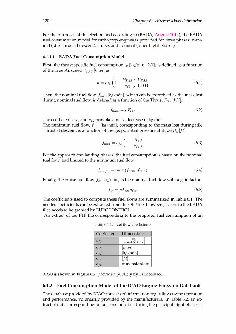
120 Chapter 6. Aircraft Mass Estimation
For the purposes of this Section and according to (BADA, August 2014), the BADAfuel consumption model for turboprop engines is provided for three phases: mini-mal (idle Thrust at descent), cruise, and nominal (other flight phases).
6.1.1.1 BADA Fuel Consumption Model
First, the thrust specific fuel consumption, µ [kg/min · kN ], is defined as a functionof the True Airspeed VTAS [knot] as
µ = cf1
(1− VTAS
cf2
)VTAS1, 000
(6.1)
Then, the nominal fuel flow, fnom [kg/min], which can be perceived as the mass lostduring nominal fuel flow, is defined as a function of the Thrust Fthr [kN ].
fnom = µFthr (6.2)
The coefficients cf1 and cf2 provoke a mass decrease in kg/min.The minimum fuel flow, fmin [kg/min], corresponding to the mass lost during idleThrust at descent, is a function of the geopotential pressure altitude Hp [ft].
fmin = cf3
(1− Hp
cf4
)(6.3)
For the approach and landing phases, the fuel consumption is based on the nominalfuel flow, and limited to the minimum fuel flow
fapp/ld = max (fnom, fmin) (6.4)
Finally, the cruise fuel flow, fcr [kg/min], is the nominal fuel flow with a gain factor
fcr = µFthrcfcr (6.5)
The coefficients used to compute these fuel flows are summarized in Table 6.1. Theneeded coefficients can be extracted from the OPF file. However, access to the BADAfiles needs to be granted by EUROCONTROL.An extract of the PTF file corresponding to the proposed fuel consumption of an
TABLE 6.1: Fuel flow coefficients
Coefficient Dimensions
cf1
[kg
min·kN ·knot
]cf2 [knot]
cf3 [kg/min]
cf4 [ft]
cfr dimensionless
A320 is shown in Figure 6.2, provided publicly by Eurocontrol.
6.1.2 Fuel Consumption Model of the ICAO Engine Emission Databank
The database provided by ICAO consists of information regarding engine operationand performance, voluntarily provided by the manufacturers. In Table 6.2, an ex-tract of data corresponding to fuel consumption during the principal flight phases is

6.1. Introduction 121
FIGURE 6.2: Performance Table file of an A320 (Eurocontrol, 2017d).
provided for a set of engines similar to the ones used for the B737-200, or its equiv-alent, the A320-200. These fuel flow models are obtained from static engine test,and each flight phase is defined only by a rough assumption of the percentage ofthrust associated to it (see Table 6.4). Furthermore, the maximum thrust providedby some engines is shown in Table 6.3. Note that this is data extracted for a singleengine, and the mentioned aircraft models posses two of them. Therefore, a fuelconsumption model using only the ICAO Engine Emission Databank will result inan interpolation based on only 4 Thrust measures with no adjustments with respectto altitude.

122 Chapter 6. Aircraft Mass Estimation
TA
BL
E6.2:FuelC
onsumption
data.
Fuelflow(kg/s)
Atm
osphericC
onditions
EngineTake-off
Clim
b-outA
pproachIdle
FuelperLTO
acycle
(kg)Barom
eter(kPa)
Temperature(K
)H
umidity
(kgw
ater/kgdry
air)V
2500-A1
1.113.924
.334.124
442101.3
286.0048
CFM
56-5-A1
1.051.862
.291.1011
38594.7-95.6
280-291.0026-.0034
CFM
56-5B41.166
.961.326
.107421
97.49-98.18283.4-293.9
.0067-.0076C
FM56-5B4/2
1.18.975
.335.121
447100.67-101.01
293-299.0114-.0129
JT8D-7
.9892.8113
.2861.1291
419-
270-311-
TA
BL
E6.3:
Maxim
umThrust
providedby
en-gines
usedin
A320-200/B737-200
EngineM
aximum
Thrust(kN)
V2500-A
1111.2
CFM
56-5-A1
111.2C
FM56-5B4
117.88C
FM56-5B4/2
117.9JT8D
-762.27
TA
BL
E6.4:
Percentageof
Thrustused
indiffer-
entflightphases
FlightPhaseThrust(%
)Take-off
100C
limb-out
85A
pproach30
Idle7
aLTOstands
forLanding/Take-O
ff.

6.2. Mass Estimations based on the longitudinal equations of motion 123
6.2 Mass Estimations based on the longitudinal equations ofmotion
The mass estimations based on the longitudinal aircraft model will be referred to asmass inferences, while the ones based on least squares (described later) as mass estima-tions, even if both are mass estimation processes. Also, for the reader’s conveniencethroughout the chapter, a non-exhaustive scheme of the mass estimation processesis provided in Figure 6.3.
According to the aircraft performance model proposed by BADA, the computa-
FIGURE 6.3: Mass estimation scheme.
tion of the lift coefficient is directly dependent on the aircraft mass, and the dragcoefficient is directly dependent on the lift (see (6.6)).
CL =2mg
ρV 2a Scos(φ)
(6.6a)
CD = CD0 + CDiC2L (6.6b)
Therefore, when these coefficients are used analytically to obtain mass inferences, acertain inaccuracy is self-induced when standard mass values are considered.In spite of the fact that this inaccuracy is corrected by taking into account observa-tions of the flown trajectory, this section describes an algorithm capable of providingmass and thrust inferences without the use of mass-dependent lift and drag coeffi-cients. Thus, the proposed approach relies on machine learning techniques, morespecifically, in the neural networks proposed in Section 4.1.3, to first estimate the liftand drag coefficients, and then infer the aircraft mass using a reduced longitudinalaircraft model. In this scenario, the training part of the neural networks becomescrucial, as it is determinant for the neural network performance.Assuming that a well-trained neural network is available for the lift and drag coeffi-cients, which could be feasible thanks to wind tunnel testing, experimental-aircraftmeasures, or any other, a mass estimation can be performed as follows.The assumption of a zero bank angle (φ ≈ 0) as well as no yawing motion (ψ ≈ 0),produce a reduced three degrees of freedom longitudinal aircraft model, expressedin the wind frame by
Va =Fthrcα −D
m− gsγ (6.7a)
γ =Fthrsα + L
mVa− g
Vacγ (6.7b)
Assuming that Va, γ and α are measured or computed at a sample time tk+1 =tk+∆t, the system (6.7) is discretized using the Euler method, such that the following

124 Chapter 6. Aircraft Mass Estimation
equations are obtained:
Vak+1= Vak + ∆t
(Fthrkcαk −Dk
mk− gsγk
)(6.8a)
γk+1 = γk + ∆t
(Fthrksαk + Lk
mkVak− g
Vakcγk
)(6.8b)
Besides, it is assumed that the aerodynamic forces D and L are known using ap-proximated models. On the other hand, the thrust force and mass are assumed tobe unknown and unmeasurable. Thus, an on-line inference of these variables can beproposed.For this purpose, (6.8a) and (6.8b) are rearranged as
Vak+1− Vak
∆t+ gsγk =
Fthrkcαk −Dk
mk(6.9a)
Vak
(γk+1 − γk
∆t
)+ gcγk =
Fthrksαk + Lkmk
(6.9b)
Then, dividing (6.9a) by (6.9b), an auxiliary variable σk is defined as
σk =Fthrkcαk −Dk
Fthrksαk + Lk(6.10a)
=
Vak+1−Vak
∆t + gsγkVak (γk+1−γk)
∆t + gcγk
(6.10b)
Hence, after manipulating (6.10a), an estimate of the thrust force at the instant tk,but computed at the instant tk+1, can be expressed as
Fthrk =Dk + σkLkcαk − σksαk
(6.11)
where σk can be computed from (6.10b). Finally, introducing (6.11) into (6.8a) and(6.8b), two possible expressions for mass inference are obtained:
m1k =Fthrkcαk −DkVak+1
−Vak∆t + gsγk
(6.12)
m2k =Fthrksαk + Lk
Vak (γk+1−γk)
∆t + gcγk
(6.13)
where m1k is feasible at any flight condition with the exception of constant speedand zero flight path angle. In this case, the m2k value can be used. Therefore, theinferred mass at the instant tk, referred to it as mk is known at the instant tk+1.In order to corroborate the feasibility of this mass inference, data corresponding tothe climb phase of a 10min simulated flight using the model described in Chapter4 was obtained. The aircraft climbs from 1, 000m to approximately 4, 000m (FL30to FL130) (see Figure 6.4), starting with an airspeed (TAS) of 100m/s (194knot) andfinishing at 122m/s (237.5kn). During the whole simulation, a pitch angle of 10 ismaintained. The variables used to infer the aircraft mass and the Thrust are shownin Figure 6.5. The quality of these data is assumed to be reliable (accurate, inte-gral, continuous and available), thanks to the use of up-to-date navaids+GNSS and

6.2. Mass Estimations based on the longitudinal equations of motion 125
FIGURE 6.4: Altitude and Rate of Climb for mass inference.
FIGURE 6.5: Variables used to infer aircraft mass and Thrust profile.
ADIRS systems.Regarding the aircraft mass, it is assumed that a measure of this parameter is
subject to uncertainty. Therefore an initial mass of 50, 000kg, decreasing under the

126 Chapter 6. Aircraft Mass Estimation
FIGURE 6.6: Fuel consumption and Thrust profile inference.
effects of a gaussian noise (with standard deviation of 100kg to avoid the simulationof an ideal measure), provoked by a fuel consumption dependent on the thrust andairspeed, is considered as the "real" mass of the aircraft during the climb. Concern-ing the "real" thrust profile, it is dependent on the altitude, speed, and drag. The fuelconsumption associated to the real mass behaviour and the inferred thrust under a12s sampling are shown in Figure 6.6. Although the generation of the thrust profileis out of the scope of this section, it must be noted that as the altitude increases, thefuel consumption and the thrust decrease, always maintaining a growing airspeed,which fits the general behaviour of aircraft during the climb phase.Regarding the mass inference, since different values of ∆t affect the inference, inFigure 6.7 are shown the results of mass inferences at different sampling times withrespect to the real mass. For a sampling at 1s, the inferred mass converges within abounded error of ±400kg, and for 2, 5, and 12s, bounds of ±300, ±300, and ±200kgare sufficient. This error reduction is thought to be related to the low-pass filter effectthat the increase in the sampling time has on the variables affected by the gaussiannoise added to avoid an ideal measure of the mass. The error of these inferenceswith respect to to an average value of the real mass (an accurate mass measure), isanalyzed later.
Hence, it could be assumed that the mass is now available for further treatment,but in addition to this, thanks to a method based on least squares and the computedmass inference, the initial mass of the aircraft can be estimated.
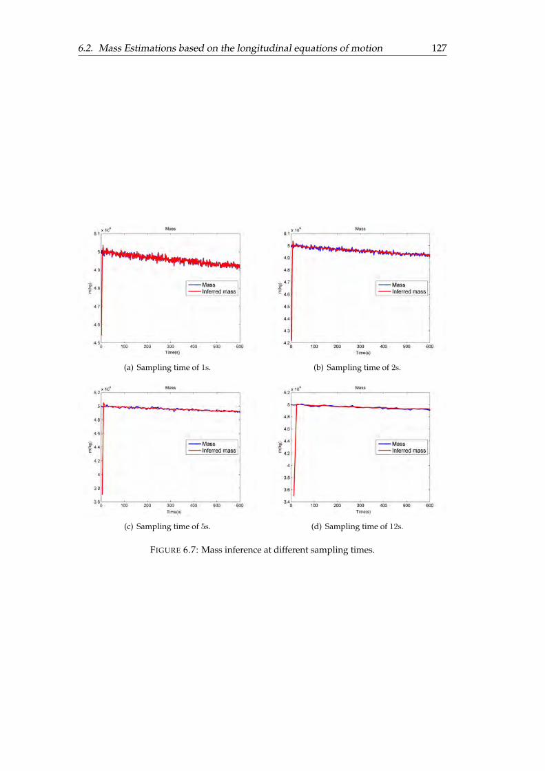
6.2. Mass Estimations based on the longitudinal equations of motion 127
(a) Sampling time of 1s. (b) Sampling time of 2s.
(c) Sampling time of 5s. (d) Sampling time of 12s.
FIGURE 6.7: Mass inference at different sampling times.

128 Chapter 6. Aircraft Mass Estimation
6.3 Mass Estimation based on Least Squares
Since the aircraft mass has been inferred repeatedly by the previous approach, refer-ring to the kth value (known at the instant tk+1) as mk. These inferences can be usedto propose an initial mass that minimizes the error (in a least squares sense) betweenthe real mass, and the inferred mass.Let the aircraft mass be modeled by the BADA expression
m = −µFthr (6.14)
where the aircraft mass decreases depending on the Thrust force and a thrust specificfuel consumption µ. This coefficient µ can be extracted from the BADA files, or theICAO engine databank.Assuming µ is measured or computed at a sample time tk+1 = tk + ∆t, the massdynamic is discretized using the Euler method, such that the following equation isobtained:
mk+1 = mk −∆tµkFthrk (6.15)
In this manner, from a general point of view, the measure of the aircraft mass can beassumed to come from the substraction of the weight of the burned fuel (given byequation (6.15)) to an unknown initial mass.Therefore, assuming that a vector of inferred masses has been computed with theapproach based on the longitudinal aircraft model in Section 6.2, the fuel consump-tion model makes possible the knowledge of the initial aircraft mass by adding allthe fuel consumed until a determined time. In other words, the initial mass of anaircraft can be estimated using a fuel consumption model and the mass inferencesknown until the instant tk+1, denoted as mk+1
0 .This is possible by minimizing the least-squared error (Els) given by
min (Els) = min
k∑l=0
[ml −
(m0 −
l∑h=0
∆thµhFthrh
)]2 ≈ 0 (6.16)
where ml is the vector containing all the mass inferences, and the term
m0 −l∑
h=0
∆thµhFthrh (6.17)
represents the real mass, given by the substraction of the weight of the burned fuel(given by equation (6.15)) to the initial mass m0, considered unknown.Hence, to solve this minimum problem, the first and second derivatives of (6.16)with respect to m0 are obtained. The first derivative is given by
2
k∑l=0
(ml −m0 +
l∑h=0
µh∆thFthrh
)k∑l=0
(−1) = 0 (6.18)
and by differentiating one more time (6.18), it is found that the second derivative ispositive
2
[k∑l=0
(−1)
]2
> 0 (6.19)

6.3. Mass Estimation based on Least Squares 129
Thus, the minimum of (6.16), is found by equalizing to zero equation (6.18) andsolving for m0, leading to
mk+10 =
1
k
[k∑l=0
(ml +
l∑h=0
∆thµhFthrh
)](6.20)
In order to test the approach, the flight simulation of the 10min climb from the pre-vious section was used. Hence, assuming a known fuel consumption, provided byBADA or the ICAO Engine Emission Databank, the initial mass estimation usingthree different sampling times (2s, 5s, and 10s) is shown in Figure 6.8. It can be seenhow as the available data to solve the least squares problem increases in size, theinitial mass estimation becomes more accurate.Moreover, the first value of the mass inferences (using the longitudinal equations)
FIGURE 6.8: Initial mass estimation.
and the initial mass estimation (using the least squares), are compared with respectto the true initial mass. This errors, named initial mass inference error, and initialmass estimation error, are compared in Figure 6.9. The superior performance of theleast squares approach at different sampling times is clear.It must be noted that the presented approach differs completely from a least squares
fitting application. If a fitting problem was considered, a polynomial function wouldbe adapted to the mass inferences, such that the polynomial describing the massevolution would dictate a fuel consumption disregarding any available prior infor-mation such as the BADA or the ICAO Engine Emission Databank model. In ourcase, the solution of a least squares method is used, but no polynomial is adjusted tofit the data.At this point, since the initial mass estimation and the fuel consumption are consid-ered known, a recalculation of the mass until the instant tk can be computed at tk+1
(using the mass dyanmic model (6.15)), denoted as mk+1kls
. This computation, willbe increasing its accuracy as every new estimation of the initial mass comes closerto the true value, this is depicted in Figure 6.10. Note that the mass estimation issmoother than the mass inference.

130 Chapter 6. Aircraft Mass Estimation
(a) Original plot (b) Zoom
FIGURE 6.9: Initial mass estimation and initial mass inference errorsat different sampling times.
Let now the error of the mass estimation (using mk+10 ) and mass inference be com-
pared with respect to an accurate mass measure (represented by the simulated realmass without the gaussian noise). These errors are shown at different samplingtimes in Figure 6.11.
FIGURE 6.10: Mass estimation using initial mass estimations.

6.3. Mass Estimation based on Least Squares 131
(a) Original plot (b) Zoom
FIGURE 6.11: Mass estimation and mass inference errors at differentsampling times.
132 Chapter 6. Aircraft Mass Estimation
6.4 Conclusions
A new method for online mass estimation, and initial mass estimation was pro-posed. The mass estimation using the longitudinal equations, despite beginning faraway from the true value, converged faster than the mass estimation based on leastsquares. However, the inclusion of initial guesses into the mass estimation based onleast squares approach could significantly improve its convergence time.The least squares approach provided an accurate initial mass estimation, not onlyequally accurate, but also smoother, compared to the mass inferences approach (massestimations using the longitudinal equations). Since the mass estimation processwas proposed as a recursive and discrete algorithm, sampling times affected the be-haviour of it.The approach to estimate the mass relied heavily on previous knowledge of the fuelconsumption model, such that the inaccuracy or complete ignorance of this param-eter would have affected severely the method. Nevertheless, an adaptive estimationof the fuel consumption model to solve this issue could be addressed.Moreover, since the fuel consumption models are well defined for the different flightphases, the method could be easily adjusted to complete flights and not limited tothe climb phase.The implementation of the proposed mass estimation methods could improve air-craft trajectory prediction, and ease the guidance efforts to follow a desired trajec-tory. In addition to this, it completed the simulation of the transport aircraft de-scribed in previous chapters.

133
Chapter 7
Introduction to Control Theory
The first feedback control system ever developed by the human being is though tobe the Egyptian water clock of Ktesibios in Alexandria, around the third century b.c.,since then, driven by curiosity, need, entertainment or even mistake, mankind hascarried on to develop new control systems regardless of the discipline throughouthistory.Nowadays, considering the ubiquity of mathematics to describe physical phenom-ena, control theory has gained great interest when a defined system, referred to asplant, need to fulfil some closed-loop behavior. In this manner, the design of a con-troller that allows a system to meet the desired characteristics has been the subjectof worldwide research.Control theory can be roughly divided in two branches, classic and modern. Thefirst one, performs an analysis of physical systems using the Laplace transform as akey tool, and the second, allows the analysis of systems based mainly on Lyapunovtheory. System analysis is done using the state-space representation, either for SISO(Single-Input/ Single-Output) or MIMO (Multi-Input/ Multi-Output) systems.According to (Slotin and Li, 1991), physical systems are nonlinear most of the time,and they can be classified in terms of their mathematical properties as continuous ordiscontinuous. In the case where the operating range to be analyzed is small, andthe nonlinearities within this range are smooth, the system may be approximated bya linear one. However, there are "hard" nonlinearities (described by discontinuousfunctions) that cannot be approximated by linear functions, such as the Coulombfriction, saturation, dead-zones, backlash, and hysteresis.In this manner, nonlinear and linear control laws are designed depending on thesystem.It is a fact that linear control laws are likely to perform poorly, or even lead to unsta-ble behaviours when large range of systems operation are required. Thus, nonlinearcontrol laws are of great interest. Furthermore, many control problems involvingmodel uncertainties can be tolerated using nonlinear control theory. Nevertheless,when a linearized system is able to represent fairly enough a nonlinear one, the com-plexity can be reduced significantly and a linear control law is sufficient.In this chapter, after providing the essentials about Linear Time-Invariant (LTI) sys-tems and Linear control techniques in Section 7.1, nonlinear systems theory and non-linear control techniques are given in Section 7.2. This background of linear / non-linear systems is stated considering that aircraft dynamics are highly nonlinear, andthat flight control systems are based on control theory, either linear or nonlinear.Moreover, the flight guidance systems of modern aircraft are briefly described inSection 7.3. Finally, conclusions are given in Section 7.4.
134 Chapter 7. Introduction to Control Theory
7.1 Linear Systems Theory
In the late 40’s, frequency response methods based on the root locus, and therefore,in the Laplace transform were developed. The root locus consists in plotting thepoles of a closed loop transfer function in the complex s-plane as a function of a gainparameter (in a feedback system). Hence, since the roots of a system change whenthe gain varies, the stability of the system can be analyzed, establishing the basis ofclassical control theory, developed by Walter R. Evans.The main contribution of the root locus analysis can be denoted by the descriptionof 1st and 2nd order linear systems.This Section is a compilation from extracts of different sources. For 1st and 2nd ordersystems (MIT, 2017) and (Ogata, 1998) are used, while (Chen, 2013) is used for thesolution, stability, controllability and observability of LTI systems.
7.1.1 First and Second Order Systems
7.1.1.1 First Order Systems
Consider any phenomenon described by a first order differential equation:
τ y(t) + y(t) = f(t) (7.1)
The system is defined by the parameter τ , referred to as the system time-constant,and f(t), which is a forcing function.It is common to separate the response of liner systems in zero-state response (initialconditions are zero), and zero-input response (input is zero).Thus, the zero-input response, or homogeneous response of (7.1) is found by settingf(t) = 0, such that using the Laplace transform
τ (sy(s)− y(0)) + y(s) = 0 (7.2a)
y(s) =y(0)
s+ 1τ
(7.2b)
where the single root λ = −1/τ provokes the system response to an initial conditiony(0):
yh(t) = y(0)eλt = y(0)e−t/τ (7.3)
Note that for τ > 0, the system behaviour is an exponential decay from the initialvalue y(0) to zero, described as an stable system. Otherwise, for τ < 0, the responsegrows exponentially, and the system is referred to as unstable.The constant τ has time units, and denotes the general behaviour of 1st order sys-tems. In this way, the homogeneous response of stable first order systems is depictedusing a normalized time t/τ , and a normalized magnitude response y(t)/y(0) in Fig-ure 7.1, where it can be seen how after a time of t = 0, τ, 2τ, 3τ, 4τ , the output reachesthe 0, 63.21, 86.47, 95.02, 98.17% of its final value, respectively.
On the other hand, the zero-state responses, or solutions to a given f(t) and theinitial condition y(0) = 0, are referred to as characteristic responses.In this way, the total response of the system (y(t)) is denoted by the sum of the ho-mogeneous solution (yh(t)) and a particular solution (yp(t)) for an input f(t), givenby:
y(t) = yh(t) + yp(t) = Ce−t/τ + yp(t) (7.4)

7.1. Linear Systems Theory 135
FIGURE 7.1: First order linear systems zero-input response (MIT,2017).
where C is a constant to be found from the initial condition.The first response analyzed is the step response (ys(t)). The step us(t) is defined forbeing us(t < 0) = 0 and us(t ≥ 0) = 1, such that the particular solution has the formyp(t) = K = 1. Then, with the requirement of ys(0) = 0, the constant C is −1. Thus,the total response of a system under a step input, is given by
ys(t) = 1− e−t/τ (7.5)
This can also be obtained from solving τ y(t) + y(t) = 1 using the laplace transformwith the initial condition ys(0) = 0.The step response is usually divided in the transient region, where the system is stillresponding dynamically, and the steady-state region, where the system has reachedits final value (yss). The initial slope of the response is 1/τ . Moreover, a normalizedresponse is given in Figure 7.2.The impulse function δ(t) is defined as a pulse of duration T and amplitude 1/T as
FIGURE 7.2: Step response of 1st order systems (MIT, 2017).

136 Chapter 7. Introduction to Control Theory
T → 0. Then, since the impulse is considered the derivative of the step function, thetotal response of a 1st order system under an impulse response is given by
yδ(t) =1
τe−t/τ for t ≥ 0 (7.6)
The normalized response is plotted in Figure 7.3.Finally, considering that the unit ramp ur(t) = t for t ≥ 0 is the integral of the unit
FIGURE 7.3: Impulse response of 1st order systems (MIT, 2017).
step, the total response of 1st order systems to a unit ramp input is obtained as
yr(t) = t− τ(
1− e−t/τ)
(7.7)
The response is plotted in Figure 7.4. Note that for large values of t compared to τ ,the exponential converges to zero, and the response becomes yr(t >> τ) = t− τ .When systems become more complex, with multiple inputs/outputs, representing
FIGURE 7.4: Unit ramp response of 1st order systems (MIT, 2017).
them with differential equations or transfer functions becomes more and more diffi-cult. Therefore, the state-space representation of a system replaces a n-order differential

7.1. Linear Systems Theory 137
equation with a single first order matrix equation.
7.1.1.2 State-Space Representation and General Solution of Linear Time Invari-ant Systems
The state-space representation of a system is given by the state equation and theoutput equation:
X(t) = A(t)X(t) +B(t)U(t) (7.8a)Y (t) = C(t)X(t) +D(t)U(t) (7.8b)
where, in the case of a nth order system (represented by an nth order differentialequation) with r inputs and m outputs, An×n is the state matrix, Bn×p is the inputmatrix, Up×1 is the input vector, Xn×1 is the state vector, Cm×n is the output matrix,Dm×p the direct transition (or feedthrough) matrix, and Ym×1 is the output vector.Linear control theory has been predominantly concerned with the study of LinearTime-Invariant (LTI) control systems, which is the case where the matrices,A,B,C,Dare constants. The Linear Time-Varying (LTV) equations are not covered in thiswork.According to (Chen, 2013), the general solution of the LTI state-space equationshinges around the exponential matrix eAt, more specifically, in the properties:
d
dteAt = AeAt = eAtA (7.9a)(
e−At)−1
= eAt (7.9b)
e0 = I (7.9c)
such that pre-multiplying both sides of (7.8a) with e−At is obtained
e−AtX(t)− e−AtAX(t) = e−AtBU(t) (7.10a)d
dt
(e−AtX(t)
)= e−AtBU(t) (7.10b)
and integrating from τ = 0 to t, yields
e−AτX(τ)|tτ=0 =
∫ t
0e−AτBU(τ)dτ (7.11a)
e−AtX(t)− e0X(0) =
∫ t
0e−AτBU(τ)dτ (7.11b)
In consequence, using the exponential matrix properties, the solution is obtained
X(t) = eAtX(0) +
∫ t
0eA(t−τ)BU(τ)dτ (7.12)
In order to verify this result, it is straightforward to check that at t = 0, the initialconditions are satisfied. Moreover, (7.12) can be differentiated using the Leibnitz’sequation, given by
d
dt
∫ β(t)
α(t)f(t, τ)dτ = f(t, β(t))
d
dtβ(t)−f(t, α(t))
d
dtα(t)+
∫ β(t)
α(t)
(d
dtf(t, τ)
)dτ (7.13)

138 Chapter 7. Introduction to Control Theory
to return to (7.8a). Furthermore, if (7.12) is substituted in (7.8b), yields
Y (t) = CeAtX(0) + C
∫ t
0eA(t−τ)BU(τ)dτ +DU(t) (7.14)
reaching the solutions of the LTI system.Note that after a similarity transformation applied to the matrix A using its eigenvectors, the exponential matrix is easily computed since the new A would be in aJordan form representation. Also, the computation of the exponential matrix can bedone using a polynomial approximation based on the Cayley-Hamilton theorem, orusing power series.Another path to reach the general solutions for LTI systems is using the Laplacetransformation to (7.8a) and (7.8b), such that
X(s) = (sI −A)−1 [X(0) +BU(s)] (7.15a)
Y (s) = C (sI −A)−1 [X(0) +BU(s)] +DU(s) (7.15b)
and by computing the inverse of Laplace, where eAt = L−1
(sI −A)−1
, the timesolution is obtained.Note that
(sI −A)−1 =1
det [sI −A]adj (sI −A) (7.16)
7.1.1.3 Second Order Systems
A 2nd order linear system can be seen as a system with a single output and two cou-pled first order differential equations expressed using two state variables, denotedby
x =
[x1
x2
]=
[a11 a12
a21 a22
] [x1
x2
]+
[b1b2
]u (7.17)
such that with the laplace transform
x(s) = (sI −A)−1Bu(s) (7.18)
it is rearranged such that
det (sI −A)x(s) =
[s− a22 a12
a21 s− a11
] [b1b2
]u (7.19)
from which
x1 − (a11 + a22) x1 + (a11a22 − a12a21)x1 = b1u+ (a12b2 − a22b1)u (7.20a)x2 − (a11 + a22) x2 + (a11a22 − a12a21)x2 = b2u+ (a21b1 − a11b2)u (7.20b)
Therefore, defining two parameters: the undamped natural frequency ωn in rad/s, andthe damping ratio ζ (dimensionless). If it is considered that
ωn =√a11a22 − a12a21 (7.21a)
ζ = − 1
2ωn(a11 + a22) (7.21b)

7.1. Linear Systems Theory 139
equations (7.20) turn into
x1 + 2ζωnx1 + ω2nx1 = b1u+ (a12b2 − a22b1)u (7.22a)
x2 + 2ζωnx2 + ω2nx2 = b2u+ (a21b1 − a11b2)u (7.22b)
Then, using the output equation, given by a scalar equation of the form
y(t) = c1x1(t) + c2x2(t) + du(t) (7.23)
It is obtained that, following a similar procedure than the one for the states:
y + 2ζωny + ω2ny = du+ (c1b1 + c2b2 − d (a11 + a22)) u+ (c1 (−a22b1 + a12b2)
+c2 (−a11b2 + a21b1) + d (a11a22 − a12a21))u (7.24)
such that the scalar form given by
y + 2ζωny + ω2ny = f(t) (7.25)
is the equation to describe 2nd order systems under a forcing input f(t).The undamped natural frequency and the damping factor play an important role inthe second order systems response, similar to the time-constant τ in first order sys-tems.In this work, the undamped natural frequency will be referred to just as natural fre-quency, unless indicated the contrary.Hence, the homogeneous solution (zero-input) of a 2nd order system equation de-noted by
y + 2ζωny + ω2ny = 0 (7.26)
is given byyh(t) = C1e
λ1t + C2eλ2t (7.27)
where C1, C2 are constants defined so the system fits the initial conditions, and theeigen values λ1, λ2 are the roots obtained from the characteristic equation:
det [sI −A] = λ2 + 2ζωnλ+ ω2n = 0 (7.28)
such thatλ1,2 = −ζωn ± ωn
√ζ2 − 1 (7.29)
In the case where ζ = 1, the two roots are equal (λ1 = λ2 = λ) such that (7.27) isreplaced by
yh2(t) = C1eλt + C2te
λt (7.30)
Thus, considering the initial conditions y(0) = y0 and y(0) = 0, the solutions of thehomogeneous system can be obtained using equations (7.27) and (7.30), along withtheir derivatives, such that
yh(0) = y0 = C1 + C2 (7.31a)yh(0) = 0 = λ1C1 + λC2 (7.31b)yh2(0) = y0 = C1 (7.31c)yh2(0) = 0 = λC1 + C2 (7.31d)
Therefore, C1 = λ2λ2−λ1 y0 and C2 = λ1
λ1−λ2 y0 are the constants for ζ 6= 1, and C1 = y0
and C2 = −λy0 otherwise.

140 Chapter 7. Introduction to Control Theory
Thus, substituting these constants in (7.27) and (7.30), the homogeneous responsefor 2nd order systems is obtained
yh(t) = y0λ1λ2
λ2 − λ1
[1
λ1eλ1t − 1
λ2eλ2t
]for ζ 6= 1 (7.32)
yh2(t) = y0
[eλt − λteλt
]for ζ = 1 (7.33)
This zero-input behaviour can be categorized depending on the damping factor.
7.1.1.3.1 Overdamped System (ζ > 1)
Two real and negative roots
λ1,2 = ωn
(−ζ ±
√ζ2 − 1
)(7.34)
When these roots are substituted in the homogeneous response (equation (7.32)), thesolution is the sum of two decaying real exponentials (with time constants −1/λ1
and −1/λ2), with no overshoot or oscillation. This response is shown in a normal-ized time and output scale in Figure 7.5.
FIGURE 7.5: Overdamped and critically damped zero-input responseof 2nd order systems with y(0) = 1 and y(0) = 0 (MIT, 2017).
7.1.1.3.2 Critically damped System (ζ = 1)
Real and identical rootsλ1,2 = ωn (7.35)
When these roots are substituted in the homogeneous response (equation (7.33)), thesolution marks the transition between the non-oscillatory response of overdampedsystems, an the oscillatory response of underdamped systems. This response isshown in Figures 7.5 and 7.6 in normalized axes.

7.1. Linear Systems Theory 141
7.1.1.3.3 Underdamped System (0 ≤ ζ < 1)
Two complex conjugate roots with negative real parts
λ1,2 = −ζωn ± jωn√
1− ζ2 = −ζωn ± jωd (7.36)
where j =√−1, and ωd = ωn
√1− ζ2 is the damped natural frequency.
When these roots are substituted in the homogeneous response (equation (7.32)), theeuler identities (involving the sin and cos with the exponential) are used to describethe response as a damped cosine function, oscillating at a ωd frequency and a decayrate of e−ζωnt. For this case, the normalized response is shown in Figure 7.6.Note that the closer the damping is to zero, the more oscillations in the response areproduced. If the damping is zero (ζ = 0), the response is a pure oscillation of theform yh(t) = y0cos(ωnt). Note also that ωd = 0 when ζ = 1.
FIGURE 7.6: Underdamped and critically damped zero-input re-sponse of 2nd order systems with y(0) = 1 and y(0) = 0 (MIT, 2017).
7.1.1.3.4 Unstable System (ζ < 0)
Two roots with real positive parts. Since the roots are on the right side of the real /complex plane, the response grows exponentially in amplitude.The root location in the real/complex plane for overdamped, underdamped, andcritically damped systems is shown in Figure 7.7.In this way, the total response of 2nd order systems is denoted by the sum of the
homogeneous solution (equations (7.27) and (7.30)) and a particular solution (yp(t))for an input f(t), such that
y(t) = C1eλ1t + C2e
λ2t + yp(t) for ζ 6= 1 (7.37)
y(t) = C1eλt + C2te
λt + yp(t) for ζ = 1 (7.38)
where C1, C2 are constants defined so the system fit the initial conditions.The total responses to step, impulse and ramp inputs, under the initial conditions ofy(0) = 0 and y(0) = 0, are summarized in Table 7.1, and Figures 7.8 and 7.9, show

142 Chapter 7. Introduction to Control Theory
(a) ζ > 1. (b) ζ = 1.
(c) ζ < 1. (d) ζ = 0.
FIGURE 7.7: Poles of 2nd order systems at different damping factors(MIT, 2017).
the normalized responses for the step and impulse functions, respectively.

7.1. Linear Systems Theory 143
FIGURE 7.8: Step response of 2nd order systems with y(0) = 0 andy(0) = 0 (MIT, 2017).
FIGURE 7.9: Impulse response of 2nd order systems with y(0) = 0and y(0) = 0 (MIT, 2017).

144 Chapter 7. Introduction to Control Theory
TABLE 7.1: Characteristic responses of y + 2ζωny + ω2ny = f(t) (MIT,
2017).
Damping Input Characteristic Response y(t)
ur(t) yr(t) = 1ω2n
[t+ e−ζωnt
ωn
(2ζcos(ωdt) + 2ζ2−1√
1−ζ2sin(ωdt)
)− 2ζ
ωn
]us(t) ys(t) = 1
ω2n
[1− e−ζωnt√
1−ζ2cos(ωdt− ψ)
]0 ≤ ζ < 1
δ(t) yδ(t) = e−ζωnt
ωn√
1−ζ2sin(ωdt)
ur(t) yr(t) = 1ω2n
[t+ 2
ωne−ωnt + te−ωnt − 2
ωn
]us(t) ys(t) = 1
ω2n
[1− e−ωnt − ωnte−ωnt
]ζ = 1
δ(t) yδ(t) = te−ωnt
ur(t) yr(t) = 1ω2n
[t+ ωn
2√
1−ζ2(τ2
1 e−t/τ1 − τ2
2 e−t/τ2
)− 2ζ
ωn
]us(t) ys(t) = 1
ω2n
[1− ωn
2√ζ2−1
(τ1e−t/τ1 − τ2e
−t/τ2)]
ζ > 1δ(t) yδ(t) = 1
2ωn√ζ2−1
(e−t/τ1 − e−t/τ2
)Notes:The damped natural frequency ωd = ωn
√1− ζ2
The phase angle ψ = tan−1(ζ/√
1− ζ2)
The time-constants τ1 = 1/(ζωn − ωn
√ζ2 − 1
)and τ2 = 1/
(ζωn + ωn
√ζ2 − 1
)

7.1. Linear Systems Theory 145
7.1.2 Stability of Linear Systems
The stability of linear systems is divided into BIBO (Bounded Input / Bounded Out-put) stability for zero-state responses, and Marginal and Asymptotic stability forzero-input responses. Again, the case of Linear Time-Varying systems is not cov-ered.
7.1.2.1 Input-Output Stability of LTI systems
Consider a proper transfer function as a ratio of two polynomials P (x)/Q(x) wherethe degree of P (x) is less than the degree of Q(x).A SISO system with a proper transfer function is BIBO stable if its impulse responseapproaches the origin (zero) as t → ∞. Also, it is BIBO stable if and only if everypole of its transfer function has a negative real part.A MIMO system is BIBO stable if and only if every component of the impulse re-sponse matrix is absolutely integrable in the interval [0,∞). This is also the case ifand only if every pole of the system has a negative real part.Consider a MIMO system, with a state-space equation (7.15b), rewritten as
Y (s) = C (sI −A)−1X(0) +[C (sI −A)−1B +D
]U(s) (7.39)
The term involving the initial condition X(0) is the zero-input (natural response)contribution to the total response, and the term involving the input U(s) is the zero-state (forced response) contribution.Hence, since BIBO stability is analyzed for the zero-state response, the transfer func-tion of the forced response is given by:
G(s) =Y (s)
U(s)=
1
det [sI −A]C [adj (sI −A)]B +D (7.40)
In this manner, the system is BIBO stable if the roots of the characteristic polynomialgiven by det [sI −A] = 0 (i.e. the poles of the system), all have negative real parts.Hence, since every pole of G(s) is an eigen value of A, if every eigen value of A hasa negative real part, then every pole has a negative real part and BIBO stability isassured. However, due to possible term cancellation in (7.40), not every eigen valueis a pole of the system. Thus, even if A has some eigen values with a zero or positivereal part, the system may still be BIBO stable.
7.1.2.2 Internal Stability of LTI systems
Regarding the zero-input response of a system, there is no difference between SISOand MIMO sytems. Consider that the state-space equations are reduced, sinceU(t) =0, such that the stability of the solution given by X(t) = eAtX(0) is analyzed.The response is marginally stable if and only if all eigen values of A have zero ornegative real parts, and those with zero real parts are simple roots of the minimalpolynomial1 of A.The response is asymptotically stable if and only if all eigen values of A have nega-tive real parts (no eigen value with zero real part is permitted).
1The minimal polynomial is the smallest (in the sense of divisibility) nonzero polynomial that thematrix satisfies. That is, if A has a minimal polynomial m(t), then m(A) = 0, and if p(t) is a nonzeropolynomial with p(A) = 0, the minimal polynomial m(t) must divide p(t).The characteristic polynomial, on the other hand, is defined algebraically. If A has a size of n × n, thecharacteristic polynomial must have a degree n. This is not true for the minimal polynomial.

146 Chapter 7. Introduction to Control Theory
In this way, asymptotical stability implies BIBO stability, and asymptotical stabilityis defined for the zero-input response of systems. BIBO stability, in general, does notimply asymptotical stability.Moreover, the asymptotic stability of the matrix A can also be checked by the Routhtest (without computing the roots), or introducing the Lyapunov equation:
A′M +MA = −N (7.41)
where A is said to be asymptotically stable if an only if any given positive definitesymmetric matrix N , has an unique symmetric solution M , and M is positive defi-nite.From this theorem, it can be extracted that the n×nmatrixA is asymptotically stableif an only if, for any given m× n matrix N with m < n and with the property
rankO = rank[N , NA . . . NAn−1
]T= n (full column rank) (7.42)
where O is an nm× n matrix, the Lyapunov equation
A′M +MA = −N ′N = N (7.43)
has a unique symmetric solution M , and M is positive definite.Furthermore, if the matrix A is asymptotically stable, the Lyapunov equation has anunique solution for every N , and the solution is given by
M =
∫ ∞0
eA′tNeAtdt (7.44)
7.1.3 Controllability and Observability of Linear Systems
Consider the state-space equation
x(t) = Ax(t) +Bu(t) (7.45a)y(t) = Cx(t) +Du(t) (7.45b)
where A, B, C, and D have a size of n× n, n× p, m× n, and m× p respectively.The first concept to be analyzed is the controllability. Since the output does notcontribute to controllability, it is neglected. The system (7.45), or the pair (A,B) issaid to be controllable if for any initial state x(0) = x0 and any final state x1, thereexists an input that transfers x0 to x1 in a finite time.This is assured if the controllability matrix
C =[B,AB,A2B, . . . , An−1B
](7.46)
has rank n (full row rank).Concerning the observability, the system (7.45) is said to be observable if for anyunknown initial state x(0), there exists a finite t1 > 0 such that the knowledge of theinput u and the output y over the interval [0, t1], suffices to determine uniquely theinitial state x(0).This is assured if the observability matrix
O =[C,CA, . . . , CAn−1
]T (7.47)

7.1. Linear Systems Theory 147
has rank n (full row rank).In addition to this, the Theorem of duality claims that the pair (A,B) is controllable ifand only if the pair (A′, B′) is observable.Further information about these topics and the proof to the given theorems is avail-able in (Chen, 2013).
7.1.4 Control Approaches of Linear Systems
The methods analyzed in this section are for the Linear Time Invariant case, and thefirst to be examined is the State-Feedback approach.
7.1.4.1 State-Feedback
This method is based on the state equation given by
x(t) = Ax(t) +Bu(t)
where the input u(t) = −Kx(t) is proposed, and the size of K is p× n. Therefore:
x(t) = Ax(t)−BKx(t) (7.48)x(t) = Ax(t) (7.49)
where A = (A−BK), such that the stability of the system is given by the roots ofthe polynomial given by
det[sI − A
](7.50)
If these roots are on the left side of the real-imaginary plane, the system is asymptot-ically stable (Hurwitz stable).Consider the system [
x1
x2
]=
[0 1−a −b
] [x1
x2
]+
[0c
]u (7.51)
choosing the input u = − [k1, k2] [x1, x2]T , the stability of the system depends on theroots of
det[sI − A
]=
[s −1
a+ ck1 s+ b+ k2c
]= 0 (7.52a)
= s2 + s(b+ ck2) + a+ ck1 = 0 (7.52b)
Thus, in order to assure the system stability
b+ ck2 > 0 a+ ck1 > 0 (7.53)
such thatk1 > −
a
ck2 > −
b
c(7.54)
In this manner, the control input given by
u =[ac
bc
] [ x1
x2
]=
1
c(ax1 + bx2) (7.55)

148 Chapter 7. Introduction to Control Theory
TABLE 7.2: Gain Computation for a PID controller (Ziegler-Nichols).
Controller kp kd kiP .5ku - -PI .45ku .54 kuTu -
PID .6ku 1.2 kuTu3kuTu
40
will guarantee the exponential stability of the system.In addition to state-feedback controllers, lead and/or lag compensators are impor-tant for classical control theory. They rely heavily in the root locus plot since theymodify the system response by introducing a pole-zero pair. These pole/zero place-ment methods help to achieve desired system specifications in terms of settling time,steady state error, rise time, damping ratio, etc.
7.1.4.2 PID control
This is a widely used feedback control method that has the main advantage of notneeding a plant model to work. Thus, for non-modeled systems, the PID controller,where PID stands for Proportional–Integral–Derivative, is of great interest. How-ever, the PID can only be implemented for SISO systems, and is very sensitive tonoise in the measured variable.This method is based on the error generated by the desired value of a variable andits measure (e(t)), such that the control input is given by
u(t) = kpe(t) + ki
∫ t
0e(τ)dτ + kde(t) (7.56)
where kp, ki, and kd are the proportional, integral, and derivative gains, respectively.These gains determine the behaviour of the closed loop system, and each gain has adifferent impact. For example, the integral term drives the overshoot and the resid-ual steady-state error that occurs with a pure proportional controller, and the deriva-tive term drives the time response of the system. In this manner, the tuning of a PIDcan result in a hard-working task when performed manually. In consequence, thegains can be computed using existing tuning methods. The most common is the oneproposed by Ziegler-Nichols.In Table 7.2 is summarized the gain computation for different PID forms based onthe Ziegler-Nichols method, where ku is the value of kp when the systems starts tooscillate (with u = kpe(t)), and Tu is the period of the oscillations provoked by ku.The Laplace form of the controller (7.56) is given by
G(s) =u(s)
e(s)= kp +
kis
+ kds =kds
2 + kps+ kis
(7.57a)
= kds2 +
kpkds+ ki
kd
s(7.57b)

7.2. Nonlinear Systems Theory 149
7.2 Nonlinear Systems Theory
This Section is a compilation of extracts from different sources, such as (Slotin andLi, 1991), (Khalil, 2002).It is a fact that the behaviour of nonlinear systems is much more complex than theone of linear systems. A clear example of that are the limit cycles (or sustainedoscillations), where the amplitude of the excitation is independent from the initialcondition, and not easily affected by parameter changes. This is completely differ-ent from the sustained oscillations of marginally stable linear systems.Another example is that besides the multiple equilibrium points of nonlinear sys-tems, the number of equilibrium points can change depending on the system pa-rameters (bifurcation). Moreover, the output of nonlinear systems is extremely sen-sitive to the initial conditions. In this way, two close initial conditions can generatecompletely different trajectories (chaos) that may change the stability of the system.In general, nonlinear systems do not satisfy the basic properties of superposition,uniqueness of an equilibrium point, or scalability of output due to an input. Thus,two principal tools for nonlinear systems are briefly described: the phase plane anal-ysis, and the Lyapunov theory.The phase plane analysis is a graphical method that allows the visualisation of thesystem behaviour without solving the nonlinear equations analytically. However, itis limited to systems of 2nd order dynamics.The basic idea of this method is to generate, in a 2D plane (phase plane portrait) withthe axes defined by the two states of the system, motion trajectories correspondingto various initial conditions, and then to obtain information concerning stability andother motion patterns of the system. The phase plane can be constructed either forlinear or nonlinear systems. The method of isoclines is widely used.On the other hand, the Lyapunov theory encompasses the direct and indirect method,introduced in the late 19th century by the Russian mathematician Alexander Lya-punov.The indirect method (or linearization method) states that the stability properties ofa nonlinear system in the vicinity of an equilibrium point are the same as those ina linearized approximation around this equilibrium point. This is the reason whylinear control laws can be used for nonlinear systems.In the same tenor, the Lyapunov’s direct method relies on the energy of a system,expressing that the motion of a mechanical system is stable if its total mechanicalenergy decreases all the time. In this manner, a scalar energy-like function (Lya-punov function) is constructed for the system, and the decrease of this function isanalyzed. The beauty of this method is the range of applicability of the concept,since its suitable to all control systems. However, this method is limited by the diffi-culty of finding the proper Lyapunov function for a given system. Lyapunov’s directmethod is considered to be the main tool for nonlinear systems analysis.Both Lyapunov’s methods form the so-called Lyapunov stability theory.
7.2.1 Autonomous Systems
In this chapter, only the Lyapunov theory for nonlinear systems is covered.Consider a nonlinear system given by
x = f(x, t) (7.58)
where f is a nonlinear vector function of size n × 1, and x is the state vector of sizen × 1. A solution x(t) corresponds to a curve in the state-space as t varies from

150 Chapter 7. Introduction to Control Theory
0→∞. This curve is referred to as the state or system trajectory.Note that even if (7.58) does not explicitly contain the control input as a variable,the equation remains the same for feedback control systems, since the input can bewritten in terms of the states and time in the closed loop dynamics.If the system does not depend explicitly on time, it is considered as autonomous,described by
x = f(x) (7.59)
otherwise, is called non-autonomous. Thus, LTI systems are autonomous and LTVnon-autonomous.Moreover, a system in the form of
x = f(x, u) = f(x) + g(x)u(t) (7.60)
is said to be an affine system.
7.2.1.1 Equilibrium point
Consider the autonomous system described by
x = f(x) (7.61)
A state x? is said to be an equilibrium point of (7.61) if once x(t) is equal to x?, itremains equal to x? ∀t ≥ t0.Matematically, this is found by solving 0 = f(x?). For example, the system denotedby x = sin(x(t)) has the equilibrium points of x?(t) = nπ for n = 0, 1, 2, 3 . . .∞.
7.2.1.2 Stability in the sense of Lyapunov
Let a spherical region BR defined by ‖x‖ < R in state-space, and SR the spheresurface, defined by ‖x‖ = R.The equilibrium point x = 0 is stable in the sense of Lyapunov if, for any R > 0,there exists r > 0 such that if ‖x(0)‖ < r, then ‖x(t)‖ < R for all t ≥ 0. Otherwise,the equilibrium point is unstable.In other words, the origin is stable in the sense of Lyapunov if a value r(R) is found,such that at time 0, the starting state within the spherical region Br, stays for the restof the trajectory x(t) within the spherical region BR. This can be expressed by
∀R > 0,∃r > 0, ‖x(0)‖ < r ⇒ ∀t ≥ 0, ‖x(t)‖ < R (7.62)
or∀R > 0,∃r > 0, x(0) ∈ Br ⇒ ∀t ≥ 0, x(t) ∈ BR (7.63)
7.2.1.3 Asymptotic and Exponential Stability
7.2.1.3.1 Asymptotic Stability
An equilibrium point x = 0 (the trivial solution) is said to be asymptotically stableif besides being stable in the sense of Lyapunov, there exists some r > 0 such that‖x(0)‖ < r implies that x(t)→ 0 as t→∞.In other words, if the system is Lyapunov stable and the limit
limt→∞
x(t, x0) = 0 ∀‖x(0)‖ < r (7.64)

7.2. Nonlinear Systems Theory 151
is true, the system is asymptotically stable.Hence, considering that a state starting within the ball Br (close to 0) converges tothe origin as time goes to infinity, the ball Br is called a domain of attraction of theequilibrium point.An equilibrium point which is Lyapunov stable but not asymptotically stable iscalled marginally stable.
7.2.1.3.2 Exponential Stability
The trivial solution of the system (x = 0) is exponentially stable if there exist twostrictly positive numbers α and λ such that
∀t > 0, ‖x(t)‖ ≤ α‖x(0)‖e−λt (7.65)
in some ball Br around the origin.In other words, the state vector converges to the origin faster than an exponentialfunction.
7.2.1.4 Local and Global Stability
The definitions of asymptotic and exponential stability concern the local stability ofsystems, since the state is considered to evolve near the trivial equilibrium point.However, if the concepts of asymptotic or exponential stability hold for any initialstate, then the equilibrium point is said to be Globally Asymptotically (or Exponen-tially) Stable.Linear asymptotic stability is always global and exponential, which explains the re-fined notions of stability at this point and not before.
7.2.1.5 Lyapunov’s Linearization Method
This method serves to analyse the local stability of a nonlinear system around anequilibrium point.It relies on the assumption that a nonlinear system behaves similarly to its linearapproximation in a range close to an equilibrium point. Therefore, based on the sta-bility of the linearized system around an equilibrium point, some inferences aboutthe stability of the nonlinear system can be extrapolated.Consider the autonomous system
x = f(x) (7.66)
Assuming that f(x) is continuously differentiable, the systems dynamics can berewritten using the Taylor series as
f(x) = f(x0) +∂f
∂x|x=x0 (x− x0) +
1
2!
∂2f
∂x2|x=x0 (x− x0)2 + fh.o.t.(x) (7.67)
152 Chapter 7. Introduction to Control Theory
where fh.o.t. stands for higher-order terms in x.Hence, since f(0) = 0, and 0 is an equilibrium point, the Jacobian matrix
A =∂f
∂x|x=0 =
∂f1∂x1
∂f1∂x2
· · · ∂f1∂xn
∂f2∂x1
∂f2∂x2
· · · ∂f2∂xn
......
. . ....
∂fn∂x1
∂fn∂x2
· · · ∂fn∂xn
(7.68)
allows to writex = Ax (7.69)
which is called the linear approximation of the original nonlinear system at the equi-librium point x = 0 (or x = x?).In case of a system
x = f(x, u) (7.70)
the Jacobian B = ∂f∂u |x=0,u=0 allows to form a system in the form x = Ax+Bu.
Thus:
• If the linearized system is strictly stable (i.e., all eigen values of A are strictlyin the left-half complex plane), the equilibrium point of the nonlinear systemis asymptotically stable.
• If the linearized system is unstable (i.e., at least one eigen value of A is strictlyin the right-half complex plane), the equilibrium point of the nonlinear systemis unstable.
• If the linearized system is marginally stable (i.e., all eigen values of A are inthe left-half complex plane, but at least one of them is on the jω axis), then noconclusion about the nonlinear system can be extracted.
7.2.1.6 Lyapunov’s Direct Method
This method is based on the total energy of a mechanical system, assuring that if theenergy is continuously dissipated, then the system, linear or nonlinear, must even-tually converge to an equilibrium point. In this manner, the stability of the system isdetermined by the analysis of a single scalar function, called the Lyapunov function(V ).Consider that zero energy corresponds to an equilibrium point. Therefore, asymp-totic stability refers to the convergence of the energy to zero, and instability is re-ferred to the growth of mechanical energy.Hence, the energy-like function has two properties:
• It is strictly positive unless the state variables are zero.
• It is associated with the system dynamics.
Consequently, some definitions are given before enouncing the Lyapunov’s directmethod.
7.2.1.6.1 Positive Definite Functions and Lyapunov Functions
Consider a ball of radiusR0. A scalar continuous function V (x) is said to be globallypositive definite if V (0) = 0 and V (x) > 0 for any x 6= 0. But is said to be locally

7.2. Nonlinear Systems Theory 153
positive definite if this is true only in a ball BR0 .Moreover, is said to be semi-positive definite if V (0) = 0 and V (x) ≥ 0 for any x 6= 0.The negative and semi-negative properties can be easily inferred.Consider the system given by
x = f(x) (7.71)
If in a ball BR0 , the function V (x) is positive definite and has continuous partialderivatives, if its time derivative along any state trajectory of the system (7.71) isnegative semi-definite (V (x) ≤ 0), then V (x) is a Lyapunov function.
7.2.1.6.2 Lyapunov theorem for Local Stability
If, in a ball BR0 , there exists a scalar function V (x) with continuous first partialderivatives such that:
• V (x) is positive definite (locally in BR0)
• V (x) is negative semi-definite (locally in BR0)
then the equilibrium point 0 is stable.But, if the derivative V (x) is locally negative definite in BR0 , then the stability isasymptotic.
7.2.1.6.3 Lyapunov theorem for Global Stability
Assume that there exists a scalar function V (x) with continuous first order deriva-tives such that
• V (x) is positive definite
• V (x) is negative definite
• V (x) is radially unbounded, meaning that V (x)→∞ as ‖x‖ → ∞
then the equilibrium at the origin is Globally Asymptotically Stable.
7.2.1.7 Invariant Set Theorems
It is very common to have a derivative of a Lyapunov function candidate V , which isonly negative semi-definite. Thus, the invariant set theorems allow to expand the Lya-punov stability concept to extract conclusions regarding the asymptotic stability todynamic behaviours, instead of just the equilibrium. For example, the convergenceto a limit cycle. This is attributed to Joseph P. La Salle.Let us define first an invariant set.A set G is an invariant set for a dynamic system if every trajectory of the systemwhich starts from a point in G remains in G for all future time. For example, anyequilibrium point is an invariant set, and the domain of attraction of an equilibriumpoint is also an invariant set.
7.2.1.7.1 Local Invariant Set Theorem
Consider an autonomous system given by
x = f(x) (7.72)

154 Chapter 7. Introduction to Control Theory
with f continuous. Also, let V (x) be a scalar function with continuous first partialderivatives.Assume that
• for some l > 0, the region Ωl defined by V (x) < l is bounded
• V (x) ≤ 0 for all x in Ωl
Let R be the set of all points within Ωl where V (x) = 0, and M be the largest invari-ant set in R. Then, every solution x(t) originated in Ωl tends to M as t→∞.Note that M is the union of all invariant sets within R (e.g., equilibrium points).Thus, if the set R is invariant (i.e., if once V = 0, then V = 0 for all future time), thenM = R. Moreover, note that V is not required to be positive definite, even if its oftenstill referred to as a Lyapunov function.A geometrical meaning of this theorem is shown in a two state example in Figure7.10, where a trajectory starting in the bounded region Ωl converges to the largestinvariant set M.
FIGURE 7.10: Convergence to the invariant set M.
7.2.1.7.2 Global Invariant Set Theorem
Consider an autonomous system given by
x = f(x) (7.73)
with f continuous. Also, let V (x) be a scalar function with continuous first partialderivatives.Assume that
• V (x)→∞ as ‖x‖ → ∞

7.2. Nonlinear Systems Theory 155
• V (x) ≤ 0 over the whole state space
Let R be the set of all points where V (x) = 0, and M be the largest invariant set inR. Then, all solutions globally asymptotically converge to M as t→∞.As stated before, the problem of finding the proper Lyapunov function for a givennonlinear system can result in a difficult task. Thus, some constructive methodshave been proposed, like the Krasovskii’s method, or the Variable Gradient method.Moreover, considering that the Lyapunov’s direct method is a method to analyse thestability of a system, it can be used to propose nonlinear controllers. The idea is topropose a scalar positive function of the system states such that using a proposedcontrol law, make the Lyapunov function decrease, assuring stability of the closedloop. In this case, the Lyapunov function can be constructed empirically or withmethods like the Sontag’s universal formula.
7.2.2 Non-autonomous Systems
In this work, only the Lyapunov’s direct method is tackled for non-autonomous sys-tems. This is due to the non applicability of La Salle’s theorems for non-autonomoussystems. On the other hand, the Barbalat’s Lemma is used.Before diving into the Barbalat’s Lemma, positive definite functions, decreasingfunctions and some points about asymptotic properties of functions and their deriva-tives are provided.
7.2.2.1 Preliminaries
A scalar time-varying function V (x, t) is locally positive definite if V (0, t) = 0 andthere exists a time-invariant positive definite function V0(x) such that
∀t ≥ t0, V (x, t) ≥ V0(x) (7.74)
Thus, a time-variant function is locally positive definite if it dominates a time-invariantlocally positive definite function. Global positive definite functions are defined sim-ilarly.A function V (x, t) is negative definite if −V (x, t) is positive definite.A function V (x, t) is positive semi-definite if it dominates a time-invariant positivesemi-definite function.A function V (x, t) is negative semi-definite if −V (x, t) is positive semi-definite.A scalar function V (x, t) is decrescent if V (0, t) = 0, and if there exists a time-invariant positive definite function Vl(x) such that
∀t ≥ 0, V (x, t) ≤ Vl(x) (7.75)
In other words, a scalar function V (x, t) is decrescent if it is dominated by a time-invariant positive definite function.Moreover, consider that for the non-autonomous system
x = f(x, t) (7.76)
and for a time-varying scalar function V (x, t), the derivative V (x, t) along the systemtrajectory is given by
dV
dt=∂V
∂t+∂V
∂xx =
∂V
∂t+∂V
∂xf(x, t) (7.77)

156 Chapter 7. Introduction to Control Theory
Regarding the asymptotic properties of functions, consider a differentiable functionf of time t. Then:
• f(t)→ 0 does not imply that f(t) converges to 0 as t→∞.
• f(t)→ 0 as t→∞ does not imply that f(t)→ 0.
• If f(t) is lower bounded and decreasing (f(t) ≤ 0), then it converges to a limit.
This result does not say wether the slope of the curve will diminish or not. Conse-quently, the Barbalat’s lemma is used to guarantee the convergence to zero of thederivative of this function.
7.2.2.2 Barbalat’s Lemma
If the differentiable function f(t) has a finite limit as t → ∞, and if f is uniformlycontinuous, then f(t)→ 0 as t→∞.A sufficient condition to check that f is uniformly continuous is to check that itsderivative is bounded. This is expressed as
∃α > 0 ∀t ≥ 0 such that ‖f(t)‖ ≤ α (7.78)
where α is a real number.Thus, using the Barbalat’s Lemma for the stability analysis of non-autonomous sys-tems, a Lyapunov’s like lemma is stated:If a scalar function V (x, t) satisfies the following conditions
• V (x, t) is lower bounded
• V (x, t) is negative semi-definite
• V (x, t) is uniformly continuous in time
then V (x, t)→ 0 as t→∞.For more information (including the proofs of the stated theorems), please refer to(Slotin and Li, 1991).
7.2.3 Control Approaches for Nonlinear systems
Several control approaches for nonlinear systems have been developed, such asnested/separated saturations, backstepping, sliding modes, adaptive control, feed-back linearization, just to mention a few. In this work, backstepping and feedbacklinearization techniques are used.Since the Backstepping is based on the Lyapunov theory, and it has already beenpresented, the approach is explained on the fly. However since the Feedback lin-earization is based on the Lie algebra and linear control techniques, it is explainedas follows.
7.2.3.1 Feedback linearization
The feedback linearization method consists in transforming algebraically a nonlinearsystem into a system with linear dynamics (Slotin and Li, 1991), (Khalil, 2002). Thisidea is demonstrated initially with a class of nonlinear systems described by the so-called companion form, or controllability canonical form, described by the dynamics
x(n) = f(x) + g(x)u(t) (7.79)

7.2. Nonlinear Systems Theory 157
where x is the scalar output of interest, u the scalar control input, and f(x), g(x) arenonlinear functions. Thus, after putting the system in a multiple-integrator form, acontrol input of the form
u =1
g(x)(v − f(x)) (7.80)
can cancel the nonlinearities and obtain a simple input-output relation in the multiple-integrator form
x(n) = v (7.81)
Then, a linear control law proposed using v = −k0x− k1x− . . .− kn−1x(n−1) assures
the system stability.Before considering a more complex system to develop the feedback linearization,some mathematical tools are provided, extracted from (Slotin and Li, 1991).
7.2.3.1.1 Lie Algebra
Given a smooth scalar function h(x) of the state vector x, mapping from Rn → R,the gradient of h is denoted by∇h
∇h =∂h
∂x(7.82)
represented by a row-vector of elements (∇h)j = ∂h/∂xj .Similarly, given a vector field f(x) in Rn (considered as a vector function mappingfrom Rn → Rn) with continuous partial derivatives, the Jacobian of f is denoted by∇f = ∂f/∂x (like in the Lyapunov’s Linearization Method), represented by a n× nmatrix of elements (∇f)ij = ∂fi/∂xj .Thus, given a smooth scalar function h(x) and a smooth vector field f(x), a scalarfunction Lfh = ∇hf is defined, called the Lie derivative of h with respect to f .Hence, the Lie derivative is the directional derivative of h along the direction of thevector f .Recursive Lie derivatives are defined as
L0fh = h (7.83a)
Lifh = Lf
(Li−1f h
)= ∇
(Li−1f h
)f (7.83b)
Similarly, if g is another vector field, the scalar function LgLfh(x) is denoted by
LgLfh = ∇ (Lfh) g (7.84)
In the same tenor, let f and g be two vector fields. The Lie bracket of f and g is avector field defined by
[f, g] = ∇gf −∇fg = adfg (7.85)
where ad stands for adjoint. Recursive Lie brackets are defined as
ad0fg = g (7.86a)
adifg =[f, adi−1
f g]
(7.86b)
The properties of the Lie brackets are the:

158 Chapter 7. Introduction to Control Theory
• Bilinearity
[α1f1 + α2f2, g] = α1 [f1, g] + α2 [f2, g]
[f, α1g1 + α2g2] = α1 [f, g1] + α2 [f, g2]
where f , f1, f2, g, g1 and g2 are smooth vector fields, and α1 and α2 are constantscalars.
• Skew-commutativity[f, g] = − [g, f ]
• Jacobi identityLadfgh = LfLgh− LgLfh
where h(x) is a smooth scalar function of x.
7.2.3.1.2 Input-Output Linearization
Consider the SISO system
x = f(x) + g(x)u (7.87a)y = h(x) (7.87b)
where f(x) is the nonlinear state equation matrix, g(x) is the controller matrix, h(x)the output matrix, u the input and y the output.The idea is to obtain and explicit dependence of the input in the output equation. Inother words, the output y is differentiated rth times until the input u appears.Hence, using the Lie derivatives
y = h(x) = L0fh(x) (7.88a)
y =∂h(x)
∂xx = Lfh(x) + Lgh(x)u (7.88b)
where, if the term Lgh(x)u = 0, means that the first derivative of y is not explicitlyrelated to the input, therefore
y = Lfh(x) (7.89)
and another differentiation needs to be done, yielding
y = L2fh(x) + LgLfh(x)u (7.90)
If LgLfh(x)u = 0, the differentiation process must continue until for some integer r
LgLr−1f h(x) 6= 0 (7.91)
where r will be called the relative degree of the system. Then, a control law of theform
u =1
LgLr−1f h(x)
(−Lrfh(x) + v
)(7.92)
is proposed, which applied to
y(r) = Lrfh(x) + LgLr−1f h(x)u (7.93)
7.2. Nonlinear Systems Theory 159
leads toy(r) = v (7.94)
In this manner, the desired dynamics of the systems are proposed in v, usually withlinear control techniques to ensure system stability.Note that r ≤ n, where n is the system order. If r = n, the input-output linearizationyields a full linearization of the system, but in the case where r < n, there willbe internal dynamics. These internal dynamics need to be bounded to ensure thestability of the system.Once the SISO case is stated, consider the MIMO case, given by the equations:
x = f(x) + g(x)u (7.95a)y = h(x) (7.95b)
where x is an n × 1 state vector, u is the m × 1 input vector (of components ui), y isthe m × 1 output vector (of components yi), f(x) and h(x) are smooth vector fields,and g(x) is an n×m matrix whose columns are smooth vector fields gi.In this case each output yi is differentiated until the inputs appear. Assume that rjis the smallest integer such that at least one of the inputs appear in y(ri)
i , then
y(ri)i = Lrif hi +
m∑j=1
LgjLri−1f hiuj (7.96)
with LgjLri−1f hi(x) 6= 0 for at least one j. This procedure for all the outputs will lead
toy
(r1)1...
y(rm)m
=
Lr1f h1(x)...
Lrmf hm(x)
+
Lg1Lr1−1f h1(x) · · · LgmL
r1−1f h1(x)
.... . .
...Lg1L
rm−1f hm(x) · · · LgmL
rm−1f hm(x)
u1
...um
(7.97)
which can be expressed as:yr = L(x) + J(x)u (7.98)
where J has to be non-singular to generate the control law given by:
u = J−1(x) (v − L(x)) (7.99)
with v = [v1, . . . , vm]T , such that, when the control law is applied to the system,yields:
y(ri)i = vi (7.100)
Thus, the desired dynamics of the system are expressed in v.In MIMO systems, the total relative degree is given by r = r1 + . . .+ rm. If the totalrelative degree is equal to n, there is no internal dynamics.

160 Chapter 7. Introduction to Control Theory
7.3 Modern Flight Guidance Systems
After the generation of a flight plan, taking into account tactical choices entered bythe crew through the Multipurpose Control Display Unit (MCDU), the aircraft isendowed with different local objectives depending on the flight phase. If these ob-jectives are to be achieved automatically, a series of guidance modes are induced bythe FMS, each one of them with different guidance variables. In other words, if theflight plan is to be followed automatically, the flight guidance system will sequencethe corresponding guidance modes using the FMS, this is called the managed modeon Airbus aircraft.On the other hand, the pilot can take over the aircraft control, and can either imposenew objectives using the Flight Control Unit (FCU) (selected mode), or modify theaircraft control surfaces using the lateral stick (manual mode).All the flight guidance functions on board modern aircraft are embedded in theFlight Management System.In addition to this, considering that the flight plan objectives are divided into lateraland vertical, the autoguidance modes are also split into lateral and vertical modes.The lateral modes use the roll angle to control the horizontal motion, and the verticalmodes use the pitch angle. The speed/thrust is controlled using the auto-thrust.Moreover, since the aircraft is an underactuated system, and the position is con-trolled by the orientation, the Flight Control Systems are also split into the Auto-matic Piloting (Autopilot) and Automatic Guidance (Autoguidance modes). In Fig-ure 7.11, a classical structure of Flight Control Systems is shown.Furthermore, the lateral guidance modes are roughly summarised as:
FIGURE 7.11: Classical structure of Flight Control Systems (Mora-Camino, 2017).
• Runway (RWY) [managed], to follow the runway centreline on take-off.
• Navigation (NAV) [managed], to capture and track the lateral guidance in theen-route phase, as well as SID and STAR routes.
• Approach (APPR) [managed], to capture and track lateral guidance for ILS andVOR during the approach.
• Go Around (GA) [managed], to track a heading reference during Go Around.
• Heading Track (HDG-TRK) [managed/selected], to capture and maintain aselected heading reference.

7.3. Modern Flight Guidance Systems 161
• Roll Out [managed], to guide the aircraft along the runway during automaticlanding.
and the vertical guidance modes as:
• Speed Reference (SRS) [managed], to maintain a speed target using the pitchangle, and guide the aircraft during take-off, initial climb and after Go-Around.
• Climb (CLB) to Descent (DES), to change altitude while maintaining speed,auto-throttle holds a constant thrust. This is known as the pitch mode, anddifferent modes are available:
1. Open climb/descent (OP CLB/DES) [selected], to reach an altitude withan open rate of climb/descent.
2. CLB/DES [managed], to level off the aircraft when reaching an altitudeconstraint.
3. Expedite climb/descent (EXP CLB/DES) [selected], which is similar toOP CLB/DES but with different speed targets.
• Altitude (ALT), to maintain the pressure altitude. Different modes are avail-able:
1. ALT and ALT*[selected], to maintain altitude when an altitude target isreached after a climb or descent. The * is for the capture mode.
2. ALT CRZ [managed], which behaves similar to ALT but the selected alti-tude has to be at or above the cruise altitude defined in the MCDU.
3. ALT CST and ALT CST* [managed], which considers a constant altitude.
• Approach (APPR) [managed], to follow the vertical flight plan. It can captureand maintain the Glide Slope of the ILS (G/S and G/S*).
• Vertical Speed (V/S) / Flight Path Angle (FPA) [selected], to maintain a de-fined vertical speed (positive or negative).
• Flare [managed], to align the aircraft with the runway centerline and adopt apitch angle to flare.
In this manner, since each autoguidance mode uses only certain guidance variables,a non-exhaustive list of the controlled variables in lateral and vertical guidance fordifferent aircrafts is given:
• Longitudinal modes
1. Normal load factor (nz) control (A320/330/340/380).
2. Pitch angle control (A300/310, B737/747/767).
3. Acquisition and hold of vertical speed and altitude.
4. Vertical profile tracking coupled with FMS (climb, cruise, descent).
5. Acquisition and hold of speed coupled with auto-throttle.
6. Acquisition and hold of path angle.
• Lateral modes
1. Roll rate acquisition (A320/330/340/380).

162 Chapter 7. Introduction to Control Theory
2. Hold of bank angle (A300/310, B737/747/767).
3. Acquisition and hold of heading.
4. Acquisition and hold of radio axis VOR or magnetic route.
5. Acquisition and hold of inertial route coupled with FMS.
Thus, each guidance mode will use different variables to control the aircraft motion.Currently, the flight guidance control laws are based on linear control techniques (P,PI, and PID controllers with scheduled gains depending on the flight conditions).However, when more control loops are added and multivariable dynamics (MIMOsystems) are considered, the controller design becomes way more complex for thisone-loop-at-a-time design.On the other hand, modern avionics systems have adopted a linearized aircraftmodel in the state-space representation, while relying on linear control techniques(state-feedback and output-feedback controllers) (Stevens and Lewis, 1992).In this work, Nonlinear Control Techniques applied to a Nonlinear aircraft modelare addressed.

7.4. Conclusion 163
7.4 Conclusion
Since modern flight guidance systems rely mainly on linear control techniques basedon the state space representation, the theory of linear systems and some linear con-trol techniques was provided.Furthermore, it seems that flight guidance systems are based on "selected" prede-fined strategies, each one of them based in a decoupled and linear aircraft model.Thus, aiming to the implementation of a 4D guidance strategy, the consideration ofa nonlinear aircraft model is mandatory, and therefore, the use of nonlinear controltechniques.In consequence, the theory corresponding to nonlinear systems has been covered,as well as the basis for nonlinear control theory. This is used to develop a completeflight guidance system with an autopilot for transport aircraft in the next chapter,which addresses the formal proposition of a 4D guidance method compliant withthe new requirements for Trajectory-Based Operations.


165
Chapter 8
4D Guidance Control for TransportAircraft
Since air traffic is predicted to increase dramatically in the upcoming years, newproblems and requirements are arising, and those related with the use of 4D trajec-tories are of most interest for this work.NextGen (FAA, 2016) and SESAR (Eurocontrol, 2016) control projects, where trafficcapacity and safety issues are central, adopt the Trajectory Based Operations (TBO)paradigm, which supposes 4D guidance effectiveness. Therefore, it is not surprisingthat an important enabler is automation, allowing aircraft to follow with more accu-racy flight plans characterized by a 4D reference trajectory.It is expected that accurate 4D guidance will improve safety by decreasing the oc-currence of near mid-air collisions for planned conflict free 4D trajectories, and thendiminish the workload associated to a single flight for air traffic controllers. Also, itwill result in a fuel usage decrease and reduced CO2 emissions per flight. Thus, theproposal of a new approach to perform 4D guidance is mandatory for the improve-ment of future guidance systems.Until today, no general control framework has been developed for 4D guidance ofa transport aircraft and current systems are extensions of 3D guidance with over-fly time constraints at some given points. In that case, control laws are based onfrequency decoupling and different PID control layers with gain scheduling provi-sions.This chapter, considers that the aircraft dynamics are composed of fast dynamics,related with the angular attitude of the aircraft, and slow dynamics, related with thetrajectory followed by the aircraft, referenced at its center of gravity.For modern transportation aircraft with Fly by Wire (FBW) technology, the autopilotis in charge of controlling the aircraft attitude, improving flying qualities throughstabilization, and generating automatic protections in dangerous piloting situations.In Section 8.1, two different approaches are studied for the autopilot, which will beconsidered to be an specific device providing in an integrated way these essentialfunctions. The approaches analyzed are based on backstepping and Non Linear In-version (NLI), both taking into account wind disturbances.Once the attitude is controlled, the attention is focused on the autoguidance system,in charge of controlling the slow flight dynamics with the aim of providing 4D guid-ance. In this manner, Section 8.2 describes two approaches based on NLI (direct andindirect). Finally, conclusions are given in Section 8.3.Numerical simulation of all control approaches is provided using Matlab.

166 Chapter 8. 4D Guidance Control for Transport Aircraft
8.1 Attitude Control
8.1.1 Backstepping
After splitting the aircraft equations in fast and slow dynamics, related with the an-gular attitude of the aircraft, and the trajectory followed by the aircraft (referenced atits center of gravity), respectively, an attitude control approach based on backstep-ping is addressed first.Backstepping architecture is an attractive approach for cascade systems, since it canproduce smooth feedback controls which are convenient for aircraft or spacecraft at-titude dynamics (Imran, Gianmarco, and Jongrae, February 2010). Furthermore, sta-bilizing nonlinearities of the system can be retained (Rajput, Weiguo, and Jingping,June 2015). Since backstepping approaches may result in trivial cancellation of termsor excessive control effort at the initial time, enhancements on the method have beendone recently. In (Kim and Kim, November 2003), it is shown that when a nonlineartracking function is proposed instead of a linear tracking function, settling times andpeak control efforts are reduced. The backstepping technique has also been appliedto design missile autopilots with model uncertainties (Mattei and Monaco, 2014),and can be combined with other control techniques like sliding-modes in order toimprove its performance (Wang, Wang, and Xiong, August 2014).Starting by considering φ and α as the link variables with the fast dynamics, in orderto integrate properly the attitude controller into a general control framework, thesevariables are controlled taking into account wind perturbations.Consider the equations presented in Chapter 3, where an expression for the angularvelocities (Ω = [p, q, r]T ) is given by:
Ω =1
2ρV 2
a SI−1
bClcCmbCn
+ Cδ
δailδeleδrud
− I−1Ω× (IΩ) (8.1)
where the inputs are the deflection of ailerons, elevator and rudder, denoted by δ =
[δail, δele, δrud]T , and ρ is the air density, α the angle of attack (AoA), β sideslip angle,
Va airspeed, S wing area, b wingspan, c mean chord, I the inertia matrix, and therolling, pitching and yawing aerodynamic coefficients (Cl, Cm, Cn, respectively) aredenoted by: Cl
CmCn
=
Clββ + Clpbp
2Va+ Clr
br2Va
Cm0 + Cmαα+ Cmqcq
2Va
Cnββ + Cnpbp
2Va+ Cnr
br2Va
(8.2)
and
Cδ =
bClδail 0 bClδrud0 cCmδele 0
bCnδail 0 bCnδrud
(8.3)
Also, the mathematical model under wind conditions for the AoA and sideslip an-gle, conformed by
[α
β
]=
[H11 H12 H13
H21 H22 H23
] pqr
+
[Q1
Q2
](8.4)

8.1. Attitude Control 167
where
H11 = −(tanβcα +
Vwycα
Vacβ
)H12 = 1 +
Vwxcα + VwzsαVacβ
H13 = −(tanβsα +
Vwysα
Vacβ
)H21 = sα +
Vwzcβ + Vwysαsβ
Va
H22 =Vwzcαsβ − Vwxsαsβ
Va
H23 = −(cα +
Vwycαsβ + Vwxcβ
Va
)
Q1 =1
Vacβ
(g1 −
1
m(L+ Fthrsα)
)+
1
Vacβ
(Vwxsα − Vwzcα
)Q2 =
1
Va
(g2 +
1
m(Y − Fthrcαsβ)
)+
1
Va
(Vwxcαsβ − Vwycβ + Vwzsαsβ
)
with
g1 = g (cαcθcφ + sαsθ)
g2 = g (cβcθsφ + sβcαsθ − sαsβcθcφ)
is complemented by the Euler equation for roll, given by
φ = p+ tgθsφq + tgθcφr (8.5)
Note that wind perturbations are included in the model as Vw = [Vwx , Vwy , Vwz ]T .
Then, a complete expression for the attitude dynamics of the aircraft is proposed as
x1 = f1(x1) + f2(x1)x2 (8.6a)x2 = f3(x1, x2) + f4(·)u (8.6b)
where x1 = [φ, α, β]T , x2 = Ω, u = δ and
f1(x1) = [0, Q1, Q2]T (8.7)
f2(x1) =
1 tgθsφ tgθcφH11 H12 H13
H21 H22 H23
(8.8)
f3(x1, x2) =1
2ρV 2
a SI−1
bClcCmbCn
− I−1Ω× (IΩ) (8.9)
f4(·) =1
2ρV 2
a SI−1Cδ (8.10)

168 Chapter 8. 4D Guidance Control for Transport Aircraft
with the Euler angles bounded as φ−π, π; θ−π2 ,
π2 ; ψ−π, π.
Hence, the problem is the control of the roll angle, AoA and sideslip angle via thecontrol surfaces. In order to tackle this issue, note that the form of the system de-noted by (8.6a), (8.6b), is the typical nonlinear affine system, where a backsteppingcontrol can be applied.Following a similar method as (Mattei and Monaco, 2014), let the error e1 = xd1 − x1
be defined under the assumption of the existence of a function ϕ(x1) such that theerror dynamics e1 = xd1 − f1(x1) − f2(x1)ϕ(x1) is Globally Asymptotically Stable inthe sense of Lyapunov under the candidate function V1(e1). Hence:
V1(e1) =∂V1(e1)
∂e1e1
=∂V1(e1)
∂e1
(xd1 − f1(x1)− f2(x1)ϕ(x1)
)≤ −W (||e1||) (8.11)
where W (||e1||) is positive definite. Then, proposing the error e2 = x2 − ϕ(x1) withthe desired values of the angular velocities as ϕ(x1), a new system in terms of errorsusing (8.6a), (8.6b) is obtained:
e1 = xd1 − f1 (x1)− f2 (x1) (e2 + ϕ(x1)) (8.12)
e2 = f3(x1, x2) + f4(·)u− ∂ϕ(x1)
∂x1[f1 (x1) + f2 (x1) (e2 + ϕ(x1))] (8.13)
Thus, from (8.12), (8.13), an augmented Lyapunov function with its derivative inorder to analyse convergence of e1 and e2 is defined as:
V2(e1, e2) = V1(e1) +1
2eT2 e2 (8.14)
V2(e1, e2) =∂V1(e1)
∂e1
[xd1 − f1 (x1)− f2 (x1) (e2 + ϕ(x1))
]+ eT2
f3(x1, x2) + f4(·)u
−∂ϕ(x1)
∂x1[f1 (x1) + f2 (x1) (e2 + ϕ(x1))]
≤ −W (||e1||)−
∂V1(e1)
∂e1f2(x1)e2 + eT2
f3(x1, x2) + f4(·)u
−∂ϕ(x1)
∂x1[f1 (x1) + f2 (x1) (e2 + ϕ(x1))]
(8.15)
Accordingly, an expression for u is chosen
u = f−14 (·)
∂ϕ(x1)
∂x1[f1(x1) + f2(x1) (e2 + ϕ(x1))] +
(∂V1(e1)
∂e1f2(x1)
)T− ke2e2 − f3(x1, x2)
(8.16)
where ke2 is a positive definite matrix gain. Then substituting (8.16) into (8.15), it isobtained
V2(e1, e2) ≤ −W (||e1||)− eT2 ke2e2 (8.17)
Moreover, in order to perform simple term cancellation, the expression for ϕ(x1) canbe selected as:
ϕ(x1) = f2(x1)−1(xd1 − f1(x1) + ke1e1
)(8.18)

8.1. Attitude Control 169
where ke1 is also a positive definite matrix gain. As a result, with the Lyapunovfunction V1(e1) = 1
2eT1 e1, (8.11) turns into:
V1(e1) = −eT1 ke1e1 (8.19)
Consequently, the system (8.12), (8.13) assume the form[e1
e2
]=
[−ke1 −f2(x1)fT2 (x1) −ke2
] [e1
e2
](8.20)
This system is Globally Asymptotically Stable using the Lyapunov function:
V (e1, e2) =1
2eT1 e1 +
1
2eT2 e2 (8.21)
such thatV (e1, e2) ≤ −eT1 ke1e1 − eT2 ke2e2 (8.22)
using the control law (8.16).Finally, LaSalle’s invariance principle is used to probe system stability.Theorem 1. LaSalle’s theorem. Let Υ be a compact (closed and bounded) set with theproperty that every solution of the system (8.6a),(8.6b), which starts in Υ remains inΥ for all future time. Let V : Υ → R (8.21) be a continuously differentiable functionsuch that V ≤ 0 in Υ. Let E be the set of all points in Υ where V (e1, e2) = 0. Let ζbe the largest invariant set in E. Then every solution starting in Υ, approaches ζ ast→∞.Proof. Convergence of e1 and e2 to zero. The proof relies on LaSalle’s theorem. Considerthe system (8.6a),(8.6b) and the radially unbounded Lyapunov function candidate(8.21). Let us define Υ = V (e1, e2) ≤ a, where a ∈ R+. Let us define the setE = (e1, e1)T ∈ Υ : V (e1, e2) = 0.Equivalently, the expression V (e1, e2) = 0 means that e1 = e2 = 0, then is easy toverify that every trajectory converges to 0 as t →∞. Therefore, the following limitsare true:
limt→∞
e1 = 0 limt→∞
e2 = 0
ensuring the converge of x1 → xd1 and x2 → xd2.A non-exhaustive block diagram of the proposed controller is shown in Figure 8.1.
FIGURE 8.1: Block diagram of the backstepping controller.

170 Chapter 8. 4D Guidance Control for Transport Aircraft
8.1.1.1 Numerical Simulation
Numerical simulations using a six DOF Matlab model were carried out in order totest the attitude controller. Sinusoidal reference signals were proposed for φ, α, andβ while wind disturbances were applied. The response of the roll angle, AoA andsideslip angle are given in Figure 8.2, while the corresponding angular velocitiesand control effort to perform these maneuvers are shown in Figure 8.3(a) and Figure8.3(b) respectively. The wind disturbances applied are Vwx = 12m/s, Vwy = 10m/sand Vwz = 6m/s, corresponding to a typical troposphere wind magnitude accordingto an ALWIN MST radar located in the Sub-Artic site (16N, 16E).
Furthermore, other numerical simulations with reference signals at different fre-
FIGURE 8.2: φ, α and β response.
(a) Angular velocities response. (b) Control Effort.
FIGURE 8.3: Attitude control behaviour.
quencies are shown in Figure 8.4 and Figure 8.5, to be sure that the attitude control

8.1. Attitude Control 171
behaves as desired. This approach is feasible thanks to the invertibility and full
(a) φ, α and β response. (b) Angular velocities response. (c) Control Effort.
FIGURE 8.4: Attitude control behaviour at different frequencies.
(a) φ, α and β response. (b) Angular velocities response. (c) Control Effort.
FIGURE 8.5: Attitude control behaviour at different frequencies.
knowledge of f2(x1) and f4(·) for regular operation limits of transport aircraft.For f2(x1) to be invertible, its determinant must be different from zero, thus
H12H23−H13H22− tgθsφ (H11H23 −H21H13)+ tgθcφ (H11H22 −H21H12) 6= 0 (8.23)
If the wind components are neglected, the condition is reduced to
− cα − tgθ (tgβsφ + cφsα) 6= 0 (8.24)
such that the matrix is invertible as long as φ 6= ±90, γ 6= ±90. It is straightforwardto infer that these conditions are never reached.In the case of f4(·), it is invertible if Cδ is invertible, such that the condition to satisfyis
b2cCmδele (ClδailCnδrud − ClδrudCnδail) 6= 0 (8.25)
Thus, the matrix is invertible as long as Cmδele 6= 0 and ClδailCnδrud−ClδrudCnδail 6= 0,which is manageable.Regarding the gain matrices ke1 and ke2 , since the analytical method to probe stabil-ity of the system (8.20) is based on Lyapunov, the values of the matrix gains wereproposed via simulation, such that:
ke1 =
9 0 00 9 00 0 9
0 ke2 =
3 0 00 5 00 0 3
At this point, the task to control the attitude of the aircraft could be considered com-pleted, even if the control surface dynamics are not included yet. However, after
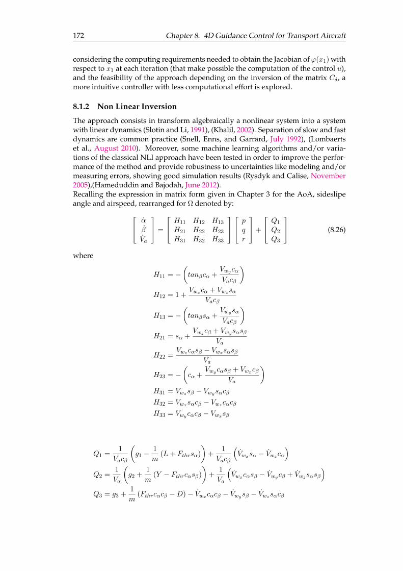
172 Chapter 8. 4D Guidance Control for Transport Aircraft
considering the computing requirements needed to obtain the Jacobian of ϕ(x1) withrespect to x1 at each iteration (that make possible the computation of the control u),and the feasibility of the approach depending on the inversion of the matrix Cδ, amore intuitive controller with less computational effort is explored.
8.1.2 Non Linear Inversion
The approach consists in transform algebraically a nonlinear system into a systemwith linear dynamics (Slotin and Li, 1991), (Khalil, 2002). Separation of slow and fastdynamics are common practice (Snell, Enns, and Garrard, July 1992), (Lombaertset al., August 2010). Moreover, some machine learning algorithms and/or varia-tions of the classical NLI approach have been tested in order to improve the perfor-mance of the method and provide robustness to uncertainties like modeling and/ormeasuring errors, showing good simulation results (Rysdyk and Calise, November2005),(Hameduddin and Bajodah, June 2012).Recalling the expression in matrix form given in Chapter 3 for the AoA, sideslipeangle and airspeed, rearranged for Ω denoted by: α
β
Va
=
H11 H12 H13
H21 H22 H23
H31 H32 H33
pqr
+
Q1
Q2
Q3
(8.26)
where
H11 = −(tanβcα +
Vwycα
Vacβ
)H12 = 1 +
Vwxcα + VwzsαVacβ
H13 = −(tanβsα +
Vwysα
Vacβ
)H21 = sα +
Vwzcβ + Vwysαsβ
Va
H22 =Vwzcαsβ − Vwxsαsβ
Va
H23 = −(cα +
Vwycαsβ + Vwxcβ
Va
)H31 = Vwzsβ − VwysαcβH32 = Vwxsαcβ − VwzcαcβH33 = Vwycαcβ − Vwxsβ
Q1 =1
Vacβ
(g1 −
1
m(L+ Fthrsα)
)+
1
Vacβ
(Vwxsα − Vwzcα
)Q2 =
1
Va
(g2 +
1
m(Y − Fthrcαsβ)
)+
1
Va
(Vwxcαsβ − Vwycβ + Vwzsαsβ
)Q3 = g3 +
1
m(Fthrcαcβ −D)− Vwxcαcβ − Vwysβ − Vwzsαcβ

8.1. Attitude Control 173
which can be written as:R = H (R) Ω +Q (R) (8.27)
Also, recalling the first-order model of the actuators, assuming δdi (i = ail, ele, rud)as the desired positions of the control surfaces, and δi as the current positions of thecontrol surfaces,
δi =1
ξi
(δdi − δi
)(8.28)
where ξi are the time-constants.Taking the angular velocities as intermediary control variables, the necessary posi-tion of the actuators (deflection of aileron, elevator and rudder) as functions of thedesired angular velocities must be determined, so the jerk vector of the angular ve-locities is obtained by differentiating one more time equation (8.1), and including(8.28), leading to p
qr
=1
2ρSI−1
V 2a
bClcCmbCn
+ Cδξ
δdail − δailδdele − δeleδdrud − δrud
+2VaVa
bClcCmbCn
+ Cδ
δailδeleδrud
− I−1In
pqr
(8.29)
with
In =
−Eq (C −B)r − Ep (C −B)q(A− C)r + 2Ep 0 (A− C)p− 2Er
(B −A)q (B −A)p+ Er Eq
and
ξ =
1ξail
0 0
0 1ξele
0
0 0 1ξrud
where the aerodynamic moment coefficients dynamics are taken into account dueto their close relation with R. On the other hand, control surfaces moment coeffi-cients dynamics are neglected. Hence, differentiating (8.2), equation (8.29) can berewritten as: p
qr
=1
2ρSI−1
V 2a Cδξ
δdail − δailδdele − δeleδdrud − δrud
+ V 2a Cc
α
β
Va
+2VaVa
bClcCmbCn
+ Cδ
δailδeleδrud
+ I−1
(1
4ρSVaCk − In
) pqr
(8.30)
where
Cc =
0 bClβ − b2
2V 2a
(Clpp+ Clrr)
cCmα 0 − c2
2V 2aCmqq
0 bCnβ − b2
2V 2a
(Cnpp+ Cnrr)

174 Chapter 8. 4D Guidance Control for Transport Aircraft
Ck =
b2Clp 0 b2Clr0 c2Cmq 0
b2Cnp 0 b2Cnr
The vector R can be taken from (8.27), and the vector Ω from (8.1). Therefore,inverting the dynamics leads to an attitude control input denoted by: δdail
δdeleδdrud
=1
V 2a
ξ−1C−1δ
2I
ρS
τpτqτr
− 2
ρS
(1
4ρSVaCk − In
) pqr
− 2VaVa
bClcCmbCn
+Cδ
δailδeleδrud
− V 2a Cc
α
β
Va
+
δailδeleδrud
(8.31)
where the wind effects appear in the terms involving α, β and Va. In consequence,the desired dynamics for the angular velocities are proposed as: τp
τqτr
=
−k1(p− pd)− k2(p− pd) + pd
−k3(q − qd)− k4(q − qd) + qd
−k5(r − rd)− k6(r − rd) + rd
(8.32)
with ki > 0 (i = 1, ...6) as gains, chosen in order to assure asymptotical convergenceof the variables to their desired values.One more time, the feasibility of the approach depends on the singularity of Cδ,the matrix involving the aerodynamic coefficients (assumed to be known thanks toexperimental data, airflow simulations, or any other method) due to the control sur-faces, aspect that can be handled.Moreover, knowing that the state is x = [p, p, q, q, r, r]T with an output y = [p, q, r]T ,and a control input u = [δail, δele, δrud]
T , each output needs to be differentiated twicefor the output to appear explicitly. Thus, the partial relative degree for each angularvelocity is two, making a total relative degree of 6, equal to the number of states.Therefore, the approach will not present internal dynamics.A non-exhaustive block diagram of the proposed controller is shown in Figure 8.6.
FIGURE 8.6: Block diagram of the NLI controller.
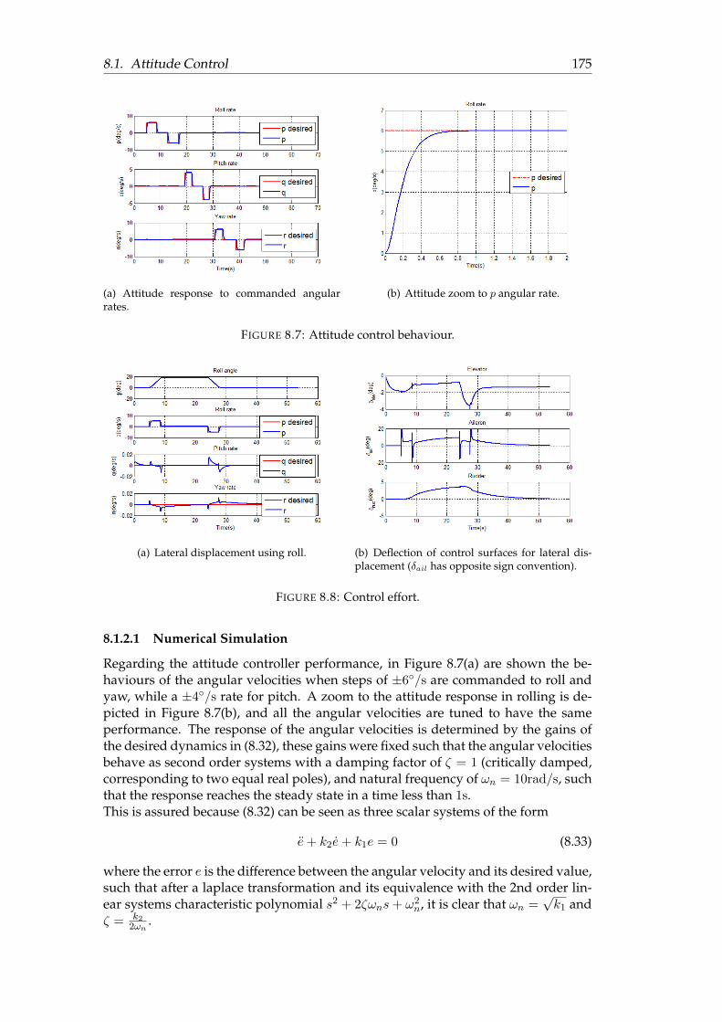
8.1. Attitude Control 175
(a) Attitude response to commanded angularrates.
(b) Attitude zoom to p angular rate.
FIGURE 8.7: Attitude control behaviour.
(a) Lateral displacement using roll. (b) Deflection of control surfaces for lateral dis-placement (δail has opposite sign convention).
FIGURE 8.8: Control effort.
8.1.2.1 Numerical Simulation
Regarding the attitude controller performance, in Figure 8.7(a) are shown the be-haviours of the angular velocities when steps of ±6/s are commanded to roll andyaw, while a ±4/s rate for pitch. A zoom to the attitude response in rolling is de-picted in Figure 8.7(b), and all the angular velocities are tuned to have the sameperformance. The response of the angular velocities is determined by the gains ofthe desired dynamics in (8.32), these gains were fixed such that the angular velocitiesbehave as second order systems with a damping factor of ζ = 1 (critically damped,corresponding to two equal real poles), and natural frequency of ωn = 10rad/s, suchthat the response reaches the steady state in a time less than 1s.This is assured because (8.32) can be seen as three scalar systems of the form
e+ k2e+ k1e = 0 (8.33)
where the error e is the difference between the angular velocity and its desired value,such that after a laplace transformation and its equivalence with the 2nd order lin-ear systems characteristic polynomial s2 + 2ζωns+ ω2
n, it is clear that ωn =√k1 and
ζ = k22ωn
.

176 Chapter 8. 4D Guidance Control for Transport Aircraft
FIGURE 8.9: Attitude response to disturbances.
The influence that a yawing motion has on the roll rate and viceversa can be nulli-fied or controlled, which plays a key roll when coordinated turns are performed.In Figure 8.8(a), a lateral displacement using roll is simulated, holding a fixed alti-tude and a constant yaw angle. In order to achieve this task, the deflection of thecontrol surfaces of the aircraft is depicted in Figure 8.8(b).Moreover, the behaviour of the attitude under some disturbances is examined byapplying wind gusts of 30m/s (58.3 knots) (see Figure 8.9).The first disturbance is applied around the fifth second in zB direction, which pro-duces an asymmetric disturbance in pitch. Then, a second disturbance is appliedaround second 10 in the−yB direction, which affects roll and yaw rates, as expected.Finally, a disturbance with components in both mentioned directions is applied ataround 21s. Note that for the moment, the error produced in position by these windgusts is not examined and only a zero angular rate is desired to be kept under thesedisturbances.Now, using the same wind disturbances like the ones used for the backstepping ap-proach, sinusoidal functions as a reference for the pitch rate, roll rate and yaw rateare simulated to test the controller behaviour.The pitch rate response is shown in Figure 8.10, where sinusoidal references of 1.5/smagnitude at different frequencies are commanded. As expected, the control effortsand the range of motion of the pitch angle change accordingly to the pitch rate.In the same way, even if the the rudder has indirect effects on the rolling motion, ne-glecting the adverse roll implies that the rudder has no direct effect in rolling. Thus,the rolling moment is completely controlled by the ailerons, and the behaviour of theroll rate is shown in Figure 8.11, where sinusoidal functions of 4/s magnitude at dif-ferent frequencies are commanded. Once again, the control efforts and the range ofthe involved euler angle change as expected.Finally, to test the yaw rate, the coupling of roll and yaw motions provoked through
the ailerons (induced yaw and adverse yaw), must be taken into account as it playsa key role in heading commands, to better understand this, lets clarify what coordi-nated/uncoordinated turns are.

8.1. Attitude Control 177
(a) Sinusoidal reference of 0.3rad/s. (b) Sinusoidal reference of 0.8rad/s.
FIGURE 8.10: Pitch rate response.
(a) Sinusoidal reference of 0.3rad/s. (b) Sinusoidal reference of 0.8rad/s.
FIGURE 8.11: Roll rate response.
8.1.2.1.1 Coordinated and Uncoordinated turns
A coordinated turn is when the bank angle of a turning aircraft complements itsturning rate. On the other hand, uncoordinated turns happen when the bank angleis too high or too low for the turning rate.When too much aileron or not enough rudder are applied in the turning direction,the bank angle is too high and the aircraft slips, causing a slipping turn with lessturning rate than expected. In this case, the nose of the airplane would be outside ofthe turn and the tail inside.Similarly, when too much rudder or not enough aileron are applied in the turningdirection, a bigger turning rate than the expected is experienced. This make the air-craft perform a skidding turn, with the tail of the aircraft outside the turn and thenose inside of it.It is common to refer to a 3/s turning rate (180/min) as a rate one turn (FAA De-cember 2015). Therefore, a rate two turn will be a 6/s turning rate (360/min).The main cause of uncoordinated turns is the non-compensation or over-compensationof the adverse yaw (banking to the left due to aileron input provokes a positiveyawing motion) and the induced yaw (a positive roll rate creates a positive yawingmotion). In both cases, uncoordinated turns will be reflected in an increase of the

178 Chapter 8. 4D Guidance Control for Transport Aircraft
airframe drag, provoking undesired turbulence, loss of performance, and uncom-fortability for passengers. Consequently, a Slip/Skid indicator (see Figure 8.12) islocated in the cockpit (either electronically in the PFD or as a physical indicator)such that pilots can perform coordinated turns easily.The roll angle to achieve a rate one turn depends on the True Air Speed of the air-
FIGURE 8.12: Slip/Skid Indicator for turn coordination. The ball tothe right indicates slip and to the left indicates skid. Only gravity
forces affect the ball position (CFI, 2017).
craft. As a rule of thumb, considering the TAS in kn, the operation (TAS/10)+7 givesthe roll angle required to achieve a rate one turn. However, at high speed, since highroll angles are undesired, ICAO (ICAO 2006b) states that "All turns are to be madeat a bank angle of 25 or at a rate of 3/s, whichever requires the lesser bank."Hence, in order to analyse the yaw rate behaviour of the controller, a rate of 2/sat 233kn TAS is commanded. It is worth to mention that during flight, constantvariations of the thrust are not desired, so thrust is considered constant for this sim-ulation. The results are shown in Figure 8.13, where it can be seen how the ruddereffort decreases as the roll angle increases, meaning that a skidding turn is beingconverted into a coordinated turn, always following the commanded 2/s yaw rate.
Note that the backstepping approach controls the roll angle, AoA, sideslip angle,and the angular velocities, while the direct NLI approach controls the angular veloc-ities. This election of link variables to the guidance controller are not coincidence.Indeed, they are chosen according to current auto-guidance modes of transport air-craft, where the normal load factor (strongly related to the pitch rate) and the rollrate, are the primary variables in both Airbus and Boeing families, making possiblethe compatibility of the proposed approaches to today’s autoguidance systems.

8.1. Attitude Control 179
FIGURE 8.13: Yaw rate step response

180 Chapter 8. 4D Guidance Control for Transport Aircraft
8.2 Guidance Control
8.2.1 Non Linear Inversion
Since the position of an aircraft is described as an underactuated motion, once theattitude controller is defined, the control structure for guidance can be proposed.Some attempts using Non Linear Inversion have been performed recently (Wahidet al., October 2014), (Wahid et al., 2016), where space-indexed trajectory trackingis done by using the rate of the euler angles and the first derivative of the thrust ascontrol inputs. Other authors have proposed to extend the energy-based control ap-proach (Lambregts, 1983) to 4D guidance (Lambregts, 1996), (Chudy and Rzucidlo,August 2009). However, some limitations appear in both cases.In the frame of direct NLI, let us first obtain the angular velocities and thrust re-quired to follow a reference trajectory. Thus, after differentiating equation (3.15),the jerk vector of the position in FE is obtained. x
(3)E
y(3)E
z(3)E
=LEBm
Fxa + FthrFyaFza
+LEBm
Fxa + FthrFyaFza
+−mm2
LEB
Fxa + FthrFyaFza
(8.34)
Considering that the mass rate of change is very small compared to the aircraft totalmass, the term containing −m
m2 is neglected. Also, writing the Euler property as
LEB = LEB
0 −r qr 0 −p−q p 0
= Mpp+Mqq +Mrr (8.35)
where
Mp =
0 cφsθcψ + sφsψ cφsψ − sφsθcψ0 cφsθsψ − sφcψ −sφsθsψ − cφcψ0 cφcθ −sφcθ
Mq =
−cφsθcψ − sφsψ 0 cθcψ−cφsθsψ + sφcψ 0 cθsψ
−cφcθ 0 −sθ
Mr =
sφsθcψ − cφsψ −cθcψ 0sφsθsψ + cφcψ −cθsψ 0
sφcθ sθ 0
and defining the vector Fab = [Fxa + Fthr, Fya , Fza ]T , equation (8.34) can be rewrittenas: x
(3)E
y(3)E
z(3)E
=1
m
cθcψMpFab MqFab cθsψ
−sθ
pq
Fthr
+1
mMrFabr +
LEBm
FxaFyaFza
(8.36)
with FxaFyaFza
=
∂Fxa∂α
∂Fxa∂β
∂Fxa∂Va
0∂Fya∂β
∂Fya∂Va
∂Fza∂α
∂Fza∂β
∂Fza∂Va
R+
∂Fxa∂ρ∂Fya∂ρ∂Fza∂ρ
ρ (8.37)

8.2. Guidance Control 181
where R is obtained from equation (8.27).Moreover, the resultant thrust produced by the engines is supposed to behave as afirst-order system, denoted by
Fthr =1
ξT
(F dthr − Fthr
)(8.38)
where the F dthr is the desired thrust and Fthr the current thrust.In this manner, taking as guidance inputs the vector [p, q, ˙Fthr]
T , the inversion of thedynamics can be proposed in the form: p
q˙Fthr
= m
cθcψMpFab MqFab cθsψ
−sθ
−1 τxτyτz
− 1
mMrFabr −
LEBm
FxaFyaFza
(8.39)
where the wind effects are involved in the vector [Fxa , Fya , Fza ]T , and the desiredbehaviour of the position is proposed as: τx
τyτz
=
−d1(x− xd)− d2(x− xd)− d3(x− xd) +...xd
−d4(y − yd)− d5(y − yd)− d6(y − yd) +...y d
−d7(z − zd)− d8(z − zd)− d9(z − zd) +...z d
(8.40)
with di > 0 (i = 1, ...9) as gains chosen in order to assure asymptotical convergenceof the variables to their desired values. For the numerical choice of these gains, (8.40)can be seen as three scalar 3rd order linear systems denoted by
...e + d3e+ d2e+ d1e = 0 (8.41)
where the error e is the difference between the position and its desired value. This3rd order system can be seen as a second order system added with an extra real poleat s3 = −1 in the Real-Imaginary plane, and its characteristic polynomial is givenby: (s2 + 2ζωns+ ω2
n)(s+ 1). Thus, a Routh-Hurwitz stability test yields:
s3
s2
s1
s0
∣∣∣∣∣∣∣∣1d3
d3d2−d1d3d1
d2
d1 (8.42)
such that the system will be stable if d3 > 0, d1 > 0, and d3d2−d1 > 0. Moreover, con-sidering the characteristic polynomial (s2 + 2ζωns+ ω2
n)(s+ 1), it is straightforwardto obtain
2ζωn + 1 = d3 (8.43)
ω2n + 2ζωn = d2 (8.44)
ω2n = d1 (8.45)
In order to have a smooth response of the aircraft position, a damping factor ζ = 1 isforced, such that s1,2 = −ωn, and s3 = −1. Also, since a slow and stable behaviour ofthe systems is needed, the poles s1,2 will be made the dominant poles of the systemby defining a ωn > 0 that satisfies the following statement:The real part of the closest poles to the imaginary axis (s1,2 = −ωn) has to be from 5

182 Chapter 8. 4D Guidance Control for Transport Aircraft
to 10 times less than the real part of the closest pole to this poles (s3 = −1). There-fore, with no zeros nearby, the poles s1,2 will be called the dominant closed looppoles, and will dominate the transient response before decay slowly.In this manner, the aircraft position response is denoted by a critically damped 2ndorder system with two equal real poles close to the imaginary axis.Values of 0.09 ≤ ωn ≤ 0.16 will make the dominant poles to be located between−0.16 ≤ s1,2 ≤ 0.09 in the Real-Imaginary plane, provoking a slow and stable be-haviour of the aircraft position response thanks to the small value of the naturalfrequency. These values of ωn satisfy the conditions obtained by the Routh-Hurwitzstability test.Moving forward, note that to develop a control law using NLI or any other model-based-approach relying on equation (8.36), the invertibility of the matrix:
MpqT =
cθcψMpFab MqFab cθsψ
−sθ
(8.46)
needs to be computed, which in the case in where φ ≈ ψ ≈ 0, the determinant of thismatrix is given by:
|MpqT |= sθFya + (sθ (Fxa + Fthr)− cθFza) (sθFza) + cθ (cθ (Fxa + Fthr) + sθFza)Fza(8.47)
and, when considered θ ≈ 0, a singularity appears for Fxa + Fthr = 0.This is the case when the plane is cruising at constant speed. Therefore, taking intoaccount that the cruise phase of a flight is essential, and that the airplane will gothrough this condition very often, any algorithm using this control approach shouldbe carefully analyzed. This result is not surprising, realizing that when a cruise flightwith the Euler angles near zero is performed, the matrix LEB will remain constant,so its derivative is expected to tend to zero. Furthermore, even if the first deriva-tive of the Euler angles along with the thrust are considered as the control inputs,[φ, θ, Fthr
]Tfor instance, as in (Wahid et al., 2016), the corresponding matrix (similar
to (8.46)) will be described by (8.48) and will also present singularities during thecruise phase.
Mφθ =
cθcψMφFab MθFab cθsψ
−sθ
(8.48)
where
Mφ = Mp
Mθ =
−sθcψ cθsφcψ cθcφcψ−sθsψ cθsφsψ cθcφsψ−cθ −sθsφ −sθcφ
A non-exhaustive block diagram of the proposed controller is shown in Figure 8.14.Furthermore, a stability proof of the proposed approach using Lyapunov theory is
provided

8.2. Guidance Control 183
FIGURE 8.14: Block diagram of the direct NLI controller.
8.2.1.1 Stability of direct NLI Guidance Control using Lyapunov theory
Lets recall equation (8.36): x(3)E
y(3)E
z(3)E
=1
mMpqT
pq
Fthr
+1
mMrFabr +
LEBm
FxaFyaFza
(8.50)
where R is obtained from equation (8.27).Rewriting (8.50) as
X(3) =M
mu+
N
m(8.51)
where
X = [xE(t), yE(t), zE(t)]T (8.52a)M = MpqT (8.52b)
N = MrFabr + LEB ·[Fxa , Fya , Fza
]T(8.52c)
u = [p, q, ˙Fthr]T (8.52d)
an intermediate variable s, non related in any way with the Laplace variable, can bedefined as
s = ¨X + 2λ ˙X + λ2X (8.53)
where λ is a 3x3 matrix containing the terms (λ1,2,3 > 0) in the diagonal. Note thatthis intermediate variable s contains the input vector in its first derivative, and theconvergence to zero of this variable as t→∞would imply that the error X = X−Xd
goes to zero. This is assured by considering that when s→ 0, equation (8.53) can beseen as three scalar 2nd order linear systems of the form
e+ 2λie+ λ2e = 0 (8.54)
where (i = 1, 2, 3), and the error e is the difference between the position and itsdesired value, such that after making the equivalence with the 2nd order linear sys-tems characteristic polynomial s2 + 2ζωns + ω2
n, it is clear that ωn = λi and ζ = 1.In this manner, each component of the error X will converge to zero as a criticallydamped 2nd order linear system with a natural frequency depending on the valuesof the matrix λ is proposed.

184 Chapter 8. 4D Guidance Control for Transport Aircraft
Then, introducing the variable Xr with its derivative as
Xr = Xd − 2λ ˙X − λ2X (8.55a)
X(3)r = Xd(3) − 2λ ¨X − λ2 ˙X (8.55b)
allows to rewrite equation (8.53) in the form
s = X − Xr (8.56)
Therefore, if a Lyapunov candidate function is proposed as
V =1
2msT s (8.57)
its derivative, mixing (8.55b) and (8.56) is expressed as
V = sTm(X(3) −X(3)
r
)(8.58a)
= sT(Mu+N −mX(3)
r
)(8.58b)
At this point, a choice of
u = M−1(−N +mX(3)
r − k1s)
(8.59)
with the positive definite matrix gain k1, would lead to V = −sTk1s. Implyingthanks to the Barbalat’s lemma that V → 0, and in consequence s → 0. Hence, thefollowing limits are true
limt→∞
¨X = 0 limt→∞
˙X = 0 limt→∞
X = 0 (8.60)
8.2.1.2 Numerical Simulation
In order to get an idea of the performance of the direct NLI, Figure 8.15(a) shows thetrajectory of the aircraft when different desired positions are commanded.The initial altitude and speed are 10,000m and 250m/s, respectively. Then, an in-crease in altitude of 100m and return to its original altitude, as well as a lateraldisplacement of 100 m and return to the original position are demanded. Next, adecrease of 10m in altitude and a lateral displacement of 50m in the opposite direc-tion to the first one are commanded. Finally, the aircraft is required to return to theoriginal altitude and original y position. The Figure 8.15(b) displays the 3D trajec-tory of the described flight.It is a key point to remark that since the control inputs for guidance are the angular
velocities, if an angular velocity is commanded for a relatively long period of time,this will result in constant and maybe undesired turning of the aircraft. One solu-tion to avoid this problem is that, when the Euler angles reach certain magnitude, theangular velocities that caused this saturation are forced to become zero until otherangular velocities in the opposite direction are commanded. The saturation of theEuler angles are: φ−30, 30; θ−15, 25; ψ−π, π.Moreover, in order to manage the singularities of the method, the desired angular

8.2. Guidance Control 185
(a) Position response to commanded positions. (b) 3D Trajectory of guidance control test.
FIGURE 8.15: Guidance control test
velocities are switched to zero when the plane goes through the cruise phase at con-stant speed.In order to analyze further the controller behaviour, the response to steps of 100min the y and z axes are depicted in Figure 8.16. The initial altitude is 1,000m and theinitial speed is 120m/s. Since the angular velocities serve as a link with the attitudecontroller, they are shown along with the corresponding euler angles. For this cases,where the thrust is kept constant, the desired values are reached in less than 50s.On the other hand, it is a fact that the response along the z axis is affected by the
(a) Lateral response. (b) Longitudinal response.
FIGURE 8.16: Guidance response to a 100m step with constant thrust.
response along the x axis. In other words, the altitude and the speed are stronglycoupled. Thus, being the thrust the principal actuator in the velocity of the aircraft,the altitude is affected by the thrust variation and vice-versa (due to the exchangebetween potential and kinetic energy of the aircraft). This is shown in Figure 8.17,where also a 100m displacement in altitude is commanded, but this time, using thethrust as control input along with the angular velocities, the behaviour of the al-titude response is modified while the convergence of the aircraft velocity to its re-quired value to provide x position control is assured.In this manner, even if the use of thrust decreases the performance in altitude andtime for this guidance approach, Figure 8.18 shows the importance of thrust as con-trol input when a bigger altitude step is commanded. This time, the desired altitude

186 Chapter 8. 4D Guidance Control for Transport Aircraft
can not be reached with the initial constant thrust (Figure 8.18(a)), but it is reachedwhen the thrust is variable (Figure 8.18(b)).Thus, the importance of the variable thrust for 4D guidance can be appreciated whencomparing the time responses of the aircraft (flying at 120m/s and 1000m altitude)required to climb 100m and 300m in Figures 8.17, 8.18(b). When the thrust is partof the control variables, the altitude has the same time response disregarding theerror magnitude (within reasonable error limits), which is, indeed, the designed be-haviour of the system for the fixed gains di > 0 (i = 1, ...9). Note the different thrustand speeds maximum values but the same altitude time response in the mentionedfigures.
FIGURE 8.17: Longitudinal response to a 100m step with a variablethrust.
(a) Constant Thrust. (b) Variable Thrust.
FIGURE 8.18: Longitudinal response to a 300m step with constant andvariable thrust.
Let now the position errors produced by wind gusts be examined, taking into ac-count that non-zero angular rates will allow the aircraft to reject perturbations andachieve the guidance objectives.In figure 8.19, wind gusts in the form of an "impulse" endowed with small turbu-lence (using a Dryden wind turbulence model) are applied, showing the effects ony and z position errors as well as the groundspeed. In this simulation, the aircraft

8.2. Guidance Control 187
is supposed to be at cruise flight at 10,000m and 250m/s velocity (≈.73Mach), suchthat the thrust applied is considered constant. Note that a thrust compensation forwind gusts could be done. However, since the wind is assumed to be a compact per-turbation in a step form, thrust and aircraft velocity are supposed to not be affectedheavily. Also, the constant thrust ensures less engine fatigue in this flight phase.
FIGURE 8.19: Position response to disturbances.
So far, the controller is assumed to have full knowledge of wind disturbances (by es-timations, measures or available forecasts), but in reality, the use of corrupted mea-surements, approximated mathematical models, or uncertainty in parameters leaveroom for errors in the control, which can be studied through a sensitivity analysis.
8.2.1.3 Sensitivity analysis with respect to wind disturbances for the direct NLIapproach
Full knowledge of variables and parameters cannot be acquired due to possiblecorrupted measures or uncertainty in parameters, leading to guidance inaccuracy.Thus, this work will provide a tool to quantify the performance of the aircraft interms of position errors due to wind gusts "impulses" by performing a sensitivityanalysis through simulation. Actuator dynamics for the control surfaces involving atime-constant are also considered.Methods to perform sensitivity analysis such as screening are common (S. Schnelle,October 2014), where a baseline experiment is done using nominal values of pa-rameters. Then, selecting two extreme values of these, the results of the perturbed

188 Chapter 8. 4D Guidance Control for Transport Aircraft
experiment with respect to the baseline are observed in order to decide to whichparameters the model is most sensitive to. Nevertheless, interaction between pa-rameters is neglected and the correlation between them and outputs of the systemis considered linear. Variance-based approaches show how to find which are themost relevant parameters and how much they affect the system output by comput-ing sensitivity indices such as Sobol indices, quantifying the amount of variancein the output caused by a parameter. These methods allow interaction of differentparameters and nonlinear responses between them and the outputs (Janon et al.,December 2014). Another technique is to compute the partial derivatives of the in-teresting variables to analyze the local sensitivity (Evans, June 2009), (Kanno et al.,September 2010).For our work, using an approach similar to the screening analysis, wind informationis used as a changing parameter to quantify the effects it has on the aircraft position.It is assumed that wind knowledge by the controller is the main contributor to po-
(a) (b)
FIGURE 8.20: Wind knowledge effect on position errors.
TABLE 8.1: Error depending on Wind knowledge
y zWind Knowledge (%) MSE MAE MSE MAE
100 10.2760 0.6731 0.7806 0.576790 8.4628 0.6787 2.0858 0.699380 13.8191 0.8001 5.8818 1.033570 23.0642 1.0926 11.7237 1.283960 35.9015 1.4416 20.3080 1.609450 55.9952 1.8394 31.2249 1.919940 78.7370 2.2092 44.1320 2.209130 107.6038 2.6044 59.4018 2.488320 140.3636 2.9848 77.5264 2.789510 177.5873 3.3675 97.0740 3.07640 220.3000 3.7540 118.4172 3.3786
sition error improvements. Note that by wind knowledge, we refer to the accuracy

8.2. Guidance Control 189
of wind gust magnitude and not the direction. So, a 70% of wind knowledge when awind gust of 10 m/s is considered, will be 7 m/s in the same direction. In this man-ner, a transport aircraft flying at 10,000m with a constant groundspeed of 250m/sunder some wind disturbances is simulated, and endowing the controller with dif-ferent wind knowledge, the position errors are examined.The aim of this analysis is to evaluate the reactiveness of an aircraft cruising at aconstant speed and a constant altitude (respecting load factor limits), when consid-erations of wind disturbances are included in the controller.The position errors for y and z with 0%, 50%, 75%, 90% and 100% of wind knowl-edge are displayed in figure 8.20, where the error magnitude decreases when windknowledge increases.This means that as the components of equation (3.31) used for the control approachtend to equations (3.32a), (3.32b), and (3.32c), the controller decreases its perfor-mance drastically, corroborating that the reactiveness of the control law (and hence,the position errors), is sensitive to wind knowledge.In Table 8.1, the Mean Squared Error (MSE) and the Mean Absolute Error (MAE) iny and z axes were computed in order to provide a clear idea of the wind sensitiv-ity with respect to aircraft position1. The disturbances, simulation time (500s), andsample time (1/30s), are the same as the ones to obtain figure 8.20.As a result, depending on each application or requirement, a maximal wind uncer-tainty can be allowed in order to do not exceed a desired error in position, proposedby the user. This wind uncertainty can be translated into wind sensors accuracy,wind estimations accuracy, or up-to-date forecasted wind.The control law used in this work can be easily replaced by other control law to com-pare their sensitivity to wind.In this manner, a safety envelope (or VoP) for a single aircraft or a group of aircraftcan be redefined, since errors will depend on wind knowledge accuracy, allowing tocreate compact aircraft clusters and decrease the workload for air traffic controllers.
8.2.2 Total Energy
In this method, the concept of a potential flight path angle denoted by: γp = γ + Vag
is considered. It indicates the potential path angle that can be achieved by bringingthe acceleration to zero by applying elevator until γ becomes γp.Since the total energy (E) is conformed by the kinetic (T ) and potential energy (V ),this yields to
E = mg
(h+
V 2a
2g
)(8.61)
and the total energy rate of change, can be expressed in terms of γp. Hence
E = Vamg
(γ +
Vag
)(8.62a)
E
Vamg= γp (8.62b)
1 The reader may notice that in Table 8.1, the MSE in y is bigger for 100% than 90% of wind knowl-edge. Even if this looks contradictory, it is explained due to the penalization of the squared errorfor high values. For example, consider the set of errors w.r.t. a reference: S100 = [1, 1, 1, 2, 10]and S90 = [1, 3, 2, 2, 9], clearly, S90 differs more from the reference than S100. However, even ifMAES100 = 3 is less than MAES90 = 3.4, as expected, the MSE is affected due to the square ofthe last value of the errors, being MSES100 = 21.4 greater than MSES90 = 19.8.
190 Chapter 8. 4D Guidance Control for Transport Aircraft
This potential flight path angle is found to be related with the specific total energyrate of the aircraft. Therefore, the approach consists in controlling the behaviour ofthe energy rate by controlling γp, using the thrust and elevator. However, the controlof this variable is performed with non available plant dynamics while introducingempirically an energy rate distribution variable to distribute the energy rate betweenthe flight path angle and acceleration. This variable is given by the first derivativeof the Langrangean (L = γ − Va
g ), assuming a constant mass, and that γ = hVa
. More-over, the distribution variable is controlled directly by the elevator, bypassing thefast dynamics and arising difficulties to integrate other autopilot functions.Furthermore, the speed and altitude dynamics in this approach are expected to beidentical, bringing to light a problem for some 4D trajectories where this is not true.Finally, no integral term has been proposed to force online position error to zero.Note that this brief analysis is only for the longitudinal motion of the plane. How-ever, the full total energy control, manages both lateral and longitudinal dynamicsas decoupled motions. Further information is available in (Lambregts, 2013), (Lam-bregts, 1983), (Lambregts, 1996), (Chudy and Rzucidlo, August 2009), (Akmeliawatiand Mareels, December 2001), and (Akmeliawati and Mareels, July 2010).
8.2.3 Guidance Control based on indirect NLI
The main objective for this 4D trajectory tracking control strategy is to avoid sin-gularity issues while inverting the flight dynamics. This will be made possible byconsidering the equations in the wind frame from Section 3.3, where the longitudinalmotion was given by:
Va =1
m(Fthrcα −D −mgsγ) (8.63)
and using the Flight Path Angle (γ = θ − α), the vertical motion was given by:
γ =1
mVa(Fthrsα + L−mgcγ) (8.64)
Also, considering that transport aircraft perform equilibrated turns, the heading rateis given by:
ψ =g
Vatgφ (8.65)
Consequently, three phases to perform the guidance control are proposed:
1. Control of the longitudinal and lateral motions, θ and φ, with stabilisation inyaw ψ.It will be considered that thanks to the relation α = θ − γ, to command θwhen γ is known, is equal to command the AoA. The control of θ and φ whilestabilizing yaw motion can be performed using classical control techniques(see Section 8.1).
2. Control of Speed and the Flight Path Angle as functions of AoA and thrustusing the guidance equations (8.63),(8.64).
3. Adjustment of the heading angle given by (8.65), targeted speed, and desiredflight path angle as functions of the positions errors generated by a 4D refer-ence trajectory.

8.2. Guidance Control 191
Proposing desired dynamics for the speed(V da
), heading
(ψd), and the flight path
angle(γd)
as first order linear responses, they are such as:
Va =1
τV
(V da − Va
)(8.66a)
γ =1
τγ
(γd − γ
)(8.66b)
ψ =1
τψ
(ψd − ψ
)(8.66c)
where τV , τγ , τψ are time-constants.Equations (8.63), (8.64), and (8.65) can be rewritten as
m
τV
(V da − Va
)+mgsγ = Fthrcα −D(ρ, α, Va) (8.67a)
mVaτγ
(γd − γ
)+mgcγ = Fthrsα + L(ρ, α, Va) (8.67b)
tg−1
(Vagτψ
(ψd − ψ
))= φ (8.67c)
Therefore, in order to obtain the values of the thrust and AoA required to follow theirproposed dynamics, the nonlinear set of equations (8.67a), (8.67b) is solved for Fthrand α. Then, saturations are applied if the results are out of the thrust
[Fminthr , F
maxthr
]and angle of attack
[αmin, αmax
]limits. Note that the Jacobian of the right hand side
of equations (8.67a), (8.67b), w.r.t. [Fthr, α]T is denoted by
J =
[cα −
(Fthrsα + ∂D(ρ,α,Va)
∂α
)sα Fthrcα + ∂L(ρ,α,Va)
∂α
](8.68)
and its determinant is
| J |= Fthr +∂L(ρ, α, Va)
∂αcα +
∂D(ρ, α, Va)
∂αsα > 0 (8.69)
In order to corroborate this, note that above the minimum flight speed:
• Thrust sign is positive during all flight.
• The derivative of Lift w.r.t. AoA is only negative in stall (never reached), andthe term cα ≥ 0 for [−π/2, π/2], ensuring a positive sign of the term.
• The derivative of Drag w.r.t. AoA is positive when α ≥ 0 and the term sα ≥ 0for [0, π/2], ensuring a positive sign of the term.
• The derivative of Drag w.r.t. AoA is negative when α < 0 but the term sα < 0for [−π/2, 0), ensuring a positive sign of the term.
Thus, it can be assured that the inversion is possible at all times.In addition to this, the φ value required to follow the lateral dynamics, it is obtaineddirectly from (8.67c), and is also saturated within the limits
[φmin, φmax
].
Therefore, in order to assure that the 4D trajectory error tends to zero after someperturbation, the reference values for Va, γ, and ψ must be adapted. The proposed

192 Chapter 8. 4D Guidance Control for Transport Aircraft
adaptive scheme is the following:
V da = Va + δVa (8.70a)
γd = γ + δγ (8.70b)
ψd = ψ + δψ (8.70c)
where
δVa =1
τx(xR − xE) (8.71a)
δγ =1
τz(zR − zE) (8.71b)
δψ =1
τy(yR − yE) (8.71c)
and τx, τy, τz are time-constants such that: τx >> τV ; τy >> τψ; τz >> τγ .The term δψ is depicted in Figure 8.21. A non-exhaustive block diagram of the
FIGURE 8.21: Change in ψ required to follow the reference trajectory
proposed controller is shown in Figure 8.22.
FIGURE 8.22: Block diagram of the indirect NLI controller.
8.2.3.1 Numerical Simulation
In order to test the proposed 4D trajectory tracking approach for the longitudinalmotion, a 100m amplitude sinusoidal reference trajectory for zR(t) is depicted in fig-ure 8.23(a). The commanded trajectory is followed with a small delay. Note that

8.2. Guidance Control 193
the numerical values of the simulation correspond to the ones predicted in Section4.2. Furthermore, a step response of a 100m error for the lateral motion is shown infigure 8.23(b).Moreover, to further analysis of the lateral motion, a 100m sinusoidal reference tra-
(a) Fthr , Va and γ required to follow a sinusoidalreference trajectory.
(b) Lateral step response for a 100m error.
FIGURE 8.23: Trajectory tracking control law simulation.
jectory of .13rad/s frequency for yR(t) is proposed, the response of the controller isdepicted in figure 8.24 along with all the variables related to the motion. For prac-tical purposes, the initial heading of the airplane is zero degrees. Besides, the delayobserved in the lateral response is due to the execution of banked turns as an un-deractuated motion, where yawing is provoked after a rolling through the aileronsonly, instead of a yawing result of a coordination of aileron-rudder.The main disadvantage of this guidance approach is that wind disturbances are not
FIGURE 8.24: Y desired stands for yR. Y stands for yE . Heading androll angles are also shown.
considered in the model. Thus, in contrast with the direct NLI algorithm, the invert-ibility guaranteed at all times comes with the lack of wind explicit considerations.

194 Chapter 8. 4D Guidance Control for Transport Aircraft
Therefore, if wind disturbances were considered, equations (8.67a), (8.67b) shouldbe substituted for:
1
τγ
(γd − γ
)=
1
mVa(L+ Fthrsα −mgcγ)− q
(Vwxcα + Vwzsα
Va
)+
1
Va
(Vwzcα − Vwxsα
)(8.72a)
1
τV
(V da − Va
)=
1
m(Fthrcα −D −mgsγ) + q (Vwxsα − Vwzcα)− Vwxcα − Vwzsα (8.72b)
such that the solution of the system of nonlinear differential equations for α andFthr, in spite of the complexity, would be of high interest.

8.3. Conclusion 195
8.3 Conclusion
Two different autopilots have been provided in this chapter, both depending on thelink variables to be used with the guidance control.The backstepping approach controls the roll angle, AoA and sideslip angle. This au-topilot is ideal in terms of compatibility with modern aircraft using the AoA and rollangle as link variables for the guidance controller. However, the computation of thecontrol law is complex, and the first order dynamics of actuators are not considered.On the other hand, the autopilot based on direct NLI assures full control of the angu-lar velocities. This autopilot is ideal when the load factors are the link variables withthe guidance controller. Moreover, the method includes the first order dynamics ofactuators, and the control law computation is less complex than the backsteppingapproach. Nevertheless, a control loop for the Euler angles is not addressed directly.Both autopilot proposals were tested in 6DOF Matlab simulations.In addition to this, two autoguidance approaches have been proposed, both depend-ing on the control input variables to be used to control the aircraft position.The first method, based on direct NLI, uses the angular velocities and the thrust rateof change as control inputs. Moreover, it provides a framework for wind sensitiv-ity analysis, where different wind uncertainties and their effects in guidance errorsare considered. In this manner, the performance of the guidance approach has beenquantified at different wind uncertainties by computing the mean squared error andmean absolute error of the aircraft position with respect to the desired position.This guidance method considers wind disturbances in the AoA and sideslip angle,as well as in airspeed. However, numerical singularities for the control law compu-tation are present at important flight phases.In the same tenor, an indirect NLI guidance control has been proposed as a secondmethod. This approach was developed such that the numerical difficulties encoun-tered by the direct NLI guidance approach are avoided. Besides, contrarily to theenergy-based methods, the independence in altitude and speed dynamics is pre-served, and the bypassing of attitude dynamics is avoided. The proposed approachuses the thrust, AoA, and bank angle as control inputs. However, the strategy doesnot include wind disturbances explicit compensation.Both guidance methods were tested in a six degrees of freedom Matlab simulation,providing satisfying results.In Table 8.2, a summary of all controllers is performed.In this manner, given a desired time-parameterized trajectory to be followed, the im-plementation of any of these guidance algorithms along with any of the autopilotsproposed, allows full 4D trajectory tracking.Future studies should consider the effects of introducing wind estimates accuracy
and the establishment of 4D trajectory tracking performance as parameters in orderto improve air traffic management.

196 Chapter 8. 4D Guidance Control for Transport Aircraft
TABLE 8.2: Controllers summary
ControllerWind considered
by controllerInvertibility at
important phasesSensitivity
analysis
Actuator dynamicsconsidered bythe controller
Backstepping(Attitude)
X X X X
NLI(Attitude)
X X X X
Direct NLI(Position)
X X X X
Indirect NLI(Position)
X X X X
197
Chapter 9
Conclusions and Perspectives
With the current increase on the air traffic demand, not only efficiency and safety ofair transport systems is threatened, but also the environmental and socio-economicconsequences linked to a failure in providing sound solutions to this arising prob-lem. In this manner, on-going research programs are allowing to tackle the enhance-ment of air traffic frameworks at different levels.This thesis is related to the transition from rigid ATC routes to flexible trajectoriesunder a 4D guidance framework, which is deeply related with the extension of theflexibility in separation between aircraft, and hence, with the increase of air traf-fic capacity under the Trajectory-Based Operations paradigm. The presented workencompassed two main contribution areas:
• Trajectory Generation.
• Flight Control Systems.
Thus, the conclusions and perspectives are also split, presenting the major actionstaken to fulfill the primary objectives of the manuscript.
9.1 General Conclusions
9.1.1 Trajectory Generation
Regarding the trajectory generation, airspace users are focused on being able to plantheir preferred routes (Business Trajectories) without being constraint by airspaceconfigurations, using published or unpublished waypoints with no relation to ATSroute networks. Thus, an approach based on Bezier curves was proposed to gener-ate 4D smooth trajectories from pre-defined control points. These trajectories wereendowed with:
• Curvature Continuity, meaning that the generated trajectory is smooth, help-ing to ease air traffic management in congested areas and improve on-boardguidance systems performance.
• Time-stamps and defined speeds for every point of the trajectory, ensuring thecompatibility with 4D guidance approaches.
• Load factor surveillance and control, thanks to considerations of the curvatureof the path and intended speed, as well as the possibility of controlling theEuclidian distance between the control points and the proposed trajectory.
• Multiplicity, meaning that parallel trajectories to a reference one are easily gen-erated.
198 Chapter 9. Conclusions and Perspectives
• Optimized Fly-by turns, as a direct consequence of the control of the distancebetween control points and the proposed trajectory.
Within these advantages, a special remark was provided concerning the load factorsurveillance. In general, the load factor that an aircraft experiences is computed us-ing its own orientation, angular velocities and linear velocity, while the trajectoryprovoking this aircraft states is disregarded.In the approach presented in this work, the trajectory generation algorithm was de-signed such that the load factor that an aircraft would experience following the gen-erated trajectory, can be obtained using the intended aircraft speed and the curvatureof the generated path. In this manner, no other aircraft state variables were requiredto obtain useful information about how the generated trajectory would impact anaircraft that intended to follow it. This not only simplified the computation time,but also avoided nominal assumption of aircraft state variables, while providingcritical information of the generated trajectory.However, the existent relation of the path curvature with the load factor that an air-craft flying the generated trajectory would experience was only given for decoupledmotions. In other words, even if the proposed approach can generate 4D trajecto-ries, only decoupled maneuvers in either lateral or vertical motions have an explicitanalytical relation of the computed curvature with the load factor. This is becausefor non-decoupled maneuvers, the expression relating the radius of the path (the in-verse of the curvature) and the load factor of an aircraft is not trivial.In this manner, the trajectory generation approach was able to generate any 4Dsmooth trajectory, but it could only analyze the load factor of those segments withindependent lateral or vertical components.Furthermore, the mathematical relation of the curvature and load factor in the ver-tical motion needed to be endowed with an external negative sign for pitch downmotions. This was because the curvature is always positive, and the differentiationbetween pitch up and down motions relies on it. In this way, the load factor wascorrectly affected. This remark concerns more to the practical implementation of thealgorithm.
9.1.1.1 Numerical Simulation of an Aircraft
Another important challenge encountered during the development of this work,was the numerical simulation of the proposed approaches using a full 6DOF air-craft model.Considering the fact that certified simulators are not free, and they do not allowthe modification of their guidance laws, the remaining option was the use of freeflight simulators. However, since many public flight simulators generally containlinearized aircraft models, they become useless for the testing of nonlinear controllaws. Hence, a full nonlinear 6DOF Matlab model was developed, similar to a B737-200 / A320-200 aircraft. No aeroelasticity, nor high lift devices were considered.A differentiation factor of the developed model, besides the full non-decoupledequations, is that the non-dimensional stability derivatives of the aircraft, insteadof being a constant value during the whole flight, they depend on multiple variablessuch as the AOA and airspeed. This was possible through the use of Neural Net-works.Moreover, the Neural Networks used to estimate the non-dimensional stability deriva-tives could allow the improvement of the aircraft model with new airborne infor-mation that could modify these derivatives, such as abnormal situations of icing,

9.1. General Conclusions 199
disfigurations in profile, major inertial matrix changes, etc. Also, the multi-input /multi-output data handling is efficient and intuitive, contrary to lookup tables.
9.1.2 Flight Control Systems
Regarding flight control systems, with the objective of diminishing the workload as-sociated to a single flight, and therefore to diminish the probability of near mid-aircollisions, two autopilots and two 4D guidance methods were developed.Regarding the autopilots, two techniques were employed, backstepping and Non-linear inversion. These autopilots were based on a complete non-decoupled aircraftmodelling, and both methods considered wind disturbances. The backstepping ap-proach controls the bank angle, AoA, and sideslip angle, while the Nonlinear inver-sion approach controls the angular velocities.In addition to this, another differentiation factor between the proposed autopilotswas that in the Nonlinear inversion approach, an explicit consideration of first orderdynamics for the deflection of the control surfaces was made, contrary to the back-stepping approach.Concerning the guidance strategies, direct Nonlinear inversion and indirect Nonlin-ear inversion techniques were used.The direct Nonlinear inversion approach considered a full 6DOF model under winddisturbances, and used the angular velocities and the thrust rate of change as con-trol inputs. However, this approach presented feasibility issues when the plane wascruising at constant speed.On the other hand, the indirect Nonlinear inversion approach used the Thrust, AoA,and bank angle as control inputs. This approach did not present feasibility issues,contrary to the direct Nonlinear inversion method, but it relied on a simplified de-coupled aircraft modelling with no wind disturbances considered.It is clear that the backstepping autopilot fits better with the guidance based on in-direct Nonlinear inversion, and that the Nonlinear inversion autopilot fits with thedirect Nonlinear inversion guidance strategy. This was due to the link variables usedfor each strategy.In summary, two different approaches for the full aircraft control were provided,each one using different link variables (See Figure 9.1).
Furthermore, since the guidance approach based on direct NLI considered wind
FIGURE 9.1: Panoramic view of the proposed control approaches.
disturbances in the control law, a sensitivity analysis of the position error w.r.t. windgusts was provided. This was performed to evaluate the reactiveness of an aircraftcruising at a constant speed and a constant altitude (respecting load factor limits).

200 Chapter 9. Conclusions and Perspectives
The analysis corroborated that the more accurate the aircraft model was consid-ered for the NLI, the better cancellation of nonlinearities was performed, and con-sequently, this led to a better control of the aircraft position. Thus, a controller ac-counting for wind disturbances would perform better than a controller with no windconsiderations.Therefore, it seems clear why the wind data available to the FMS is a determinantfactor for a substantial impact on the implementation of TBO. In this manner, asafety envelope (or VoP) for a single aircraft or a group of aircrafts could be re-defined in terms of the wind known to the FMS, and this wind uncertainty couldbe translated into wind sensors accuracy, wind estimations accuracy, or up-to-dateforecasted wind. Thus, aircraft position errors would depend on wind knowledgeaccuracy, allowing to create compact aircraft clusters and decrease the workload forair traffic controllers.Note that a method to perform wind estimations was out of the scope of this work.The quality of data to feed the attitude and guidance control algorithms was as-sumed to be reliable (accurate, integral, continuous and available), thanks to the useof up-to-date navaids, GNSS and ADIRS systems.
9.1.2.1 Aircraft Mass Estimation
Moreover, it was assumed that an inaccurate aircraft mass has significant conse-quences in trajectory optimization, fuel consumption, and aircraft performance, suchthat two mass estimation methods were proposed.
• The first method relies on the knowledge of the Drag and Lift forces and mea-sures of some longitudinal variables. This approach uses a reduced and de-coupled longitudinal aircraft model to compute the aircraft mass.
• The second method uses the vector of mass estimations of the first method tocompute the initial mass of the aircraft by solving a least squares problem, andthen recalculates the aircraft mass estimation. This approach relies completelyon the knowledge of a fuel consumption model.
These mass estimation algorithms, even if they are tested just for the climb phase,could be easily extended to full flights, such that the benefits of better trajectoryprediction and ease of guidance efforts to follow a desired trajectory, could also bespread to a complete flight. Moreover, since the control approaches rely on the in-version of dynamics, the knowledge of an accurate mass helped to a more exactnumerical inversion.In general terms, these mass estimation methods were conceived to complete thesimulation of a transport aircraft, seeking to ease the guidance efforts to follow adesired trajectory. This was expected since the Nonlinear inversion guidance ap-proaches rely on a numerical inversion of the aircraft model. Therefore, a betterknowledge of the aircraft parameters (like the aircraft mass), helps to improve thenumerical inversion accuracy of the approach, leading to a better guidance perfor-mance.

9.2. Future Work 201
9.2 Future Work
9.2.1 Trajectory Generation
Many improvements could be performed to the presented work. Concerning trajec-tory generation, the proposed approach was endowed with the capacity to generatea full flight profile without being decoupled in lateral and vertical profiles. In thismanner, a conflict analysis between different trajectories could be further analyzed.Considering that the Bezier curves are polynomials, a conflict identification methodcould be implemented by solving a system of equations formed by the polynomialsof different trajectories for different aircraft. Thus, if two polynomials have a so-lution, an intersection of the polynomials is inherent. Therefore, the time-stamp ofeach trajectory at the intersection moment could be used to analyze the possibilityof a conflict, and address it if present.
9.2.1.1 Numerical Simulation of an Aircraft
Moreover, the neural networks trained for the numerical computation of the non-dimensional stability derivatives of the aircraft could be retrained periodically dur-ing flight, such that abnormal conditions modifying the aircraft model dynamicscould be taken into account. This online training would allow to spread the useof these approach for more than transport aircraft. For example, a fighter aircraftafter taking damage in its structure will present significant changes in its stabilityderivatives, impossible to predict. Thus, the neural networks could be retrained totake into account such modifications and not only ease the performance of the flightguidance system, but also to identify the remaining handling capabilities, and ad-vert the pilot for critical aircraft performance. Note that this periodical training ofthe neural networks would be directly related to the evolution from supervised tounsupervised learning.
9.2.2 Flight Control Systems
Regarding the control approaches, since aircraft are expected to fly in compact flowcorridors, a confidence area to assure safety in operations could be defined using thesensitivity analysis with respect to wind disturbances. This protection area could bedynamic and asymmetric depending on wind knowledge and direction. An exam-ple of this protection area for different wind directions is shown in Figure 9.2.
FIGURE 9.2: Dynamic protection area depending on wind direction.

202 Chapter 9. Conclusions and Perspectives
9.2.2.1 Aircraft Mass Estimation
In terms of the mass estimation methods, a better assessment of the proposed algo-rithms could be performed with data obtained from real flights and not only simula-tions. However, in spite of the fact that the proposed simulated data is unlikely to beobserved in real traffic, it served perfectly to show the methodology of the approachproposed, which was the ultimate goal.

203
Appendix A
Coordinate Transformations
This appendix is based on (Etkin and Reid, 1996).
A.1 Transformation of a Vector
Let a vector v be a vector with components va = [va1, va2, va3]T and vb = [vb1, vb2, vb3]T
expressed in the reference frames Fa = [xa1, xa2, xa3]T and Fb = [xb1, xb2, xb3]T , re-spectively. Both reference frames share the location of its origin.The component va1 in the direction of xbi is denoted by va1cθi1 , where θi1 denotesthe angle between the axes xbi and xa1. Therefore, taking into account the othercomponents of va in the direction of xbi, it is obtained that
vbi =3∑j=1
lijvaj i = 1, 2, 3 (A.1)
withlij = cθij (A.2)
as the nine director cosinus, such that
vb1 = cθ11va1 + cθ12va2 + cθ13va3 (A.3a)vb2 = cθ21va1 + cθ22va2 + cθ23va3 (A.3b)vb3 = cθ31va1 + cθ32va2 + cθ33va3 (A.3c)
Thus, a vector va is expressed in the frame Fb by using the director cosinus. In otherwords, each component of va is related with the three axes xbi.Consequently, the matrix form of (A.3) is given by
vb = Lbava =
l11 l12 l13
l21 l22 l23
l31 l32 l33
va (A.4)
The matrix Lba belongs to the SO3 group, so the transpose of the matrix equals to itsinverse
(L−1ba = LTba = Lab
), yielding
vb = Lbava (A.5)va = Labvb (A.6)
Since va and vb represent physically the same vector v, but just seen from differentreference frames, the magnitude should be the invariant, such that
v2 = vTb vb = vTa LTbaLbava = vTa va (A.7)

204 Appendix A. Coordinate Transformations
For this equation to be satisfied, it must be true that LTbaLba = I .Moreover, if several transformations through several frames of reference are per-formed, for example from Fa to Fc passing through Fb, the consecutive rotationsare
vb = Lbava (A.8)vc = Lcbvb = LcbLbava (A.9)
such thatvc = Lcava (A.10)
withLca = LcbLba (A.11)
A.2 The Rotation Matrix
The transformations associated with single rotations about the three coordinate axesare given. In each case, let Fa be the original frame and Fb the frame after one singlerotation. Hence, in each case, vb = Li(Xi)va, so different cosinus director L matricesare obtained. Using the mnemonic to obtain the angle θij that the subindex i is theaxe after the rotation (the one belonging to Fb), and j is the original axe (the onebelonging to Fa), a rotation around the axe xa1 (see Figure A.1), leads to a matrix
FIGURE A.1: Basic rotation about xa1.
L1(X1) =
c0 c90 c90
c90 cX1 c(90−X1)
c90 c(X1+90) cX1
=
1 0 00 cX1 sX1
0 −sX1 cX1
(A.12)
Analogously, the rotations around the axes xa2 and xa3, described by the angles X2
and X3, respectively, provide the matrices
L2(X2) =
cX2 0 −sX2
0 1 0sX2 0 cX2
(A.13)
L3(X3) =
cX3 sX3 0−sX3 cX3 0
0 0 1
(A.14)

A.3. Transformation of the Derivative of a vector 205
Finally, the rotation matrix for any sequence of rotations can be constructed from theabove basic formulas. For the case of the Euler angles, which rotate from the frameFE into the frame FB , the matrix corresponding to the sequence (X3, X2, X1) =(ψ, θ, φ), is given by
LBE = L1(φ)L2(θ)L3(ψ) (A.15)
which results in the rotation matrix from the Earth to Body frame:
LBE =
cθcψ cθsψ −sθsφsθcψ − cφsψ sφsθsψ + cφcψ sφcθcφsθcψ + sφsψ cφsθsψ − sφcψ cφcθ
(A.16)
A.3 Transformation of the Derivative of a vector
First, it is useful to consider the cross product by minors of two vectors a = [a1, a2, a3]T
and b = [b1, b2, b3]T , such that
c = a× b =
i j ka1 a2 a3
b1 b2 b3
=
a2b3 − a3b2a3b1 − a1b3a1b2 − a2b1
= ab (A.17)
where
a =
0 −a3 a2
a3 0 −a1
−a2 a1 0
(A.18)
is an skew symmetric matrix. This matrix has all its entries of the main diagonal aszero, such that the trace is also zero, and it holds the property of aT = −a.Stated this, the transformation of coordinates of the derivative of a vector using arotation matrix is given as follows.Assume that a vector v is observed simultaneously in two reference frames Fa andFb, and consider that the frame Fb rotates with angular velocity ω relative to Fa,which may be regarded as fixed, then
vb = Lbava (A.19)
or analogouslyva = Labvb (A.20)
The derivatives of va and vb are va = [va1, va2, va3]T and vb = [vb1, vb2, vb3]T , respec-tively. Therefore, the derivative of (A.19) is
vb = Lbava + Lbava (A.21)
or analogouslyva = Labvb + Labvb (A.22)
Since L must be independent of v, the matrix Lab can be obtained from (A.22) byconsidering the case when vb constant, leading to
va = Labvb (A.23)
Moreover, the derivative of v seen from the frame Fa is denoted by
va = ωava (A.24)

206 Appendix A. Coordinate Transformations
such that from (A.23), (A.24), and (A.20), it is obtained
Lab = ωaLab (A.25)
If this argument is repeated with Fb considered fixed and Fa moving with an angularvelocity −ω, the reciprocal result is reached
Lba = −ωbLba (A.26)
Thus, from the transpose of (A.25) and (A.26) it is obtained
ωa = LabωbLba (A.27)
Finally, if (A.25) and (A.27) are used in (A.22), the following expression is found
Lbava = vb + ωbvb (A.28)

207
Appendix B
Gaussian Distribution
B.1 Mathematical Representation
B.1.1 Univariate Gaussian Distribution
One of the most important probability distribution is the Gaussian or Normal distri-bution. For a single real-valued variable x, is defined by
N (x|µ, σ2) =1
(2πσ2)1/2exp
− 1
2σ2(x− µ)2
(B.1)
where µ is the mean, and σ2 is the variance. The square root of the variance, givenby σ, is called the standard deviation, and the reciprocal of the variance, given byβ = 1/σ2, the precision. The Gaussian distribution satisfies
N (x|µ, σ2) > 0 (B.2)∫ ∞−∞N (x|µ, σ2)dx = 1 (B.3)
So it is said to be a valid probability density. The average value of x under a Gaussiandistribution is denoted by
E [x] =
∫ ∞−∞N (x|µ, σ2)xdx = µ (B.4)
Since the parameter µ represents the average value, it is referred to as the mean.Similarly
E[x2]
=
∫ ∞−∞N (x|µ, σ2)x2dx = µ2 + σ2 (B.5)
and hence, from (B.4), (B.5), it is obtained
var [x] = E[x2]− E [x]2 = σ2 (B.6)
therefore, σ2 is referred to as the variance parameter. For a Gaussian distribution,the mode coincides with the mean.
B.1.2 Multivariate Gaussian Distribution
A Gaussian distribution defined over a D−dimensional vector x of continuous vari-ables is denoted by
N (x|µ,Σ) =1
(2π)D/21
|Σ|1/2exp
−1
2(x− µ)T Σ−1 (x− µ)
(B.7)

208 Appendix B. Gaussian Distribution
where the D−dimensional vector µ is the mean, and the D × D matrix Σ is thecovariance. The determinant of Σ is denoted by |Σ|.

B.2. Regression applied to a Gaussian distribution using the Maximum Likelihoodapproach
209
B.2 Regression applied to a Gaussian distribution using theMaximum Likelihood approach
Let assume a data set of observations X = (x1, . . . , xN )T , representing N obser-vations of a scalar variable x. It can be supposed that the observations are takenindependently from a Gaussian distribution whose mean µ and variance σ2 are un-known, and the goal is to determine these parameters from the data set.Knowing that the joint probability of two independent events is given by the prod-uct of the marginal probabilities for each event separately, the probability of the dataset, given µ and σ2, can be written in the form
p(X|µ, σ2) =N∏n=1
N (xn|µ, σ2) (B.8)
Note that when it is viewed as a function of µ and σ, this is the likelihood functionfor the Gaussian distribution.To determinate the parameters of the probability distribution using an observed dataset, the parameters to be found will be the ones that maximize the likelihood func-tion. This is using the frequentist criterion of maximize the probability of the datagiven the parameters and not the Bayesian criterion of maximize the probability ofthe parameters given the data.From (B.1) and (B.8), the logarithmic function is denoted by
lnp(X|µ, σ2) = − 1
2σ2
N∑n=1
(xn − µ)2 − N
2lnσ2 − N
2ln(2π) (B.9)
Maximizing (B.9) w.r.t. µ, it is obtained the maximum likelihood solution given by
µML =1
N
N∑n=1
xn (B.10)
which is the sample mean. Similarly, maximizing (B.9) w.r.t. σ2, it is obtained themaximum likelihood for the variance
σ2ML =
1
N
N∑n=1
(xn − µML)2 (B.11)
which is the sample variance measured w.r.t. the sample mean µML. Since the maxi-mum likelihood solutions are functions of the data set values x1, . . . , xN , the expec-tations of these solutions are
E [µML] = µ (B.12)
E[σ2]
=
(N − 1
N
)σ2 (B.13)
showing that the maximum likelihood estimate will underestimate the true varianceby a factor (N − 1)/N , so the unbiased estimate for the variance is given by
σ2 =N
N − 1σ2ML =
1
N − 1
N∑n=1
(xn − µML)2 (B.14)

210 Appendix B. Gaussian Distribution
Note that the bias of the maximum likelihood solution becomes less significant as Ngrows.

211
Appendix C
Neural Networks Performance
In this Appendix, the performance of the neural networks developed to fit the nondi-mensional stability derivatives databases from the DATCOM software are presented.This performance is given in terms of the Mean Squared Error of the proposed curvewith respect to the training and testing data sets.
FIGURE C.1: Performance of the proposed CL coefficient.
FIGURE C.2: Performance of the proposed CYβ coefficient.

212 Appendix C. Neural Networks Performance
FIGURE C.3: Performance of the proposed Clβ coefficient.
FIGURE C.4: Performance of the proposed Clp coefficient.
FIGURE C.5: Performance of the proposed Clr coefficient.

Appendix C. Neural Networks Performance 213
FIGURE C.6: Performance of the proposed Cmα coefficient.
FIGURE C.7: Performance of the proposed Cmq coefficient.
FIGURE C.8: Performance of the proposed Cnβ coefficient.

214 Appendix C. Neural Networks Performance
FIGURE C.9: Performance of the proposed Cnp coefficient.
FIGURE C.10: Performance of the proposed Cnr coefficient.

215
List of Publications
• H. Escamilla Núñez, F. Mora Camino, H. Bouadi. “Towards 4D TrajectoryTracking for Transport Aircraft”. 20th International Federation of Automatic Con-trol World Congress (IFAC WC). Toulouse, France. 9-14 July 2017.DOI: https://doi.org/10.1016/j.ifacol.2017.08.1268.
• H. Escamilla Núñez, H. Bouadi, F. Mora Camino. “A Framework for WindSensitivity Analysis for Trajectory Tracking”. American Institute of Aeronauticsand Astronautics Guidance, Navigation, and Control Conference (AIAA GNC). Gay-lord Texan Convention Center, Grapevine, Texas, USA. 9-13 January 2017.DOI: http://dx.doi.org/10.2514/6.2017-1726.
• H. Escamilla Núñez, F. Mora Camino. “Generation of Curvature ContinuousTrajectories for Transport Aircraft using Bezier Curves”. 19th International Con-ference New Trends in Civil Aviation 2017 (NTCA). Prague, Czech Republic. 7-8December 2017.ISBN: 978-0-8153-7602-6.
• H. Escamilla Núñez, F. Mora Camino. “Generation of Smooth Reference Tra-jectories for Transport Aircraft”. 16th Simpósio de Transporte Aéreo (SITRAER).Rio de Janeiro, Brazil. 25-27 October 2017.


217
Bibliography
Akmeliawati, Rini and Iven M. Y. Mareels (December 2001). “Nonlinear Energy-Based Control Method for Aircraft Dynamics”. In: Proceedings of the 40th IEEEConference on Decision and Control (CDC). DOI: 10.1109/CDC.2001.980179.
— (July 2010). “Nonlinear Energy-Based Control Method for Aircraft AutomaticLanding Systems”. In: IEEE Transactions on Control Systems Technology 18.4, pp. 871–884.
Alligier, R., D. Gianazza, and N. Durand (December 2015). “Machine learning andmass estimation methods for ground-based aircraft climb prediction”. In: IEEETransactions on Intelligent Transportation Systems 16.6, pp. 3138–3148.
— (June 2013). “Ground-based estimation of the aircraft mass, adaptive vs. leastsquares method”. In: 10th USA/Europe Air Traffic Management Research and Devel-opment Seminar, pp. 1–10.
— (May 2012). “Energy Rate Prediction Using an Equivalent Thrust Setting Profile”.In: 5th International Conference on Research in Air Transportation (ICRAT), Berkeley,USA.
— (November 2013). “Learning the aircraft mass and thrust to improve the ground-based trajectory prediction of climbing flights”. In: Transportation Research Part C:Emerging Technologies 36, pp. 45–60. DOI: https://doi.org/10.1016/j.trc.2013.08.006.
Alligier, R. et al. (May 2014). “Comparison of Two Ground-based Mass EstimationMethods on Real Data”. In: 6th International Conference on Research in Air Trans-portation (ICRAT), Istanbul, Turkey.
Anderson, Erik P., Randal W. Beard, and Timothy W. McLain (May 2005). “Real-timedynamic trajectory smoothing for unmanned air vehicles”. In: IEEE Transactionson Control Systems Technology 13.3. DOI: 10.1109/TCST.2004.839555.
AWC (2017). US Department of Commerce. National Oceanic and Atmospheric Adminis-tration. Aviation Weather Center. URL: http://www.aviationweather.gov/.
BADA (August 2014). User Manual for the Base of Aircraft Data. English. Version Re-vision 3.12, EEC Technical/Scientific Report No. 14/04/24-44. European Organ-isation for the Safety of Air Navigation. Eurocontrol.
Bakolas, Efstathios, Yiming Zhao, and Panagiotis Tsiotras (August 2011). “InitialGuess Generation for Aircraft Landing Trajectory Optimization”. In: AIAA Guid-ance, Navigation, and Control Conference, Portland, Oregon, USA. DOI: http://dx.doi.org/10.2514/6.2011-6689.
Barsky, Brian A. and Tony D. DeRose (October 1984). “Geometric continuity of Para-metric Curves. Technical Report No. UCB/CSD 84/205”. In: University of Berke-ley, USA.
Bishop, Christopher M. (2006). Pattern Recognition and Machine Learning. Springer.CFI (2017). URL: http://www.cfinotebook.net/notebook/avionics-and-
instruments/turn-coordinator.Chati, Yashovardhan S. and Hamsa Balakrishnan (June 2017). “Statistical Modeling
of Aircraft Takeoff Weight”. In: Twelfth USA/Europe Air Traffic Management Re-search and Development Seminar (2017 ATM R&D), Seattle, Washington, USA.

218 BIBLIOGRAPHY
Chen, Chi-Tsong (2013). Linear System Theory and Design. 4th edition. Madison Av-enue, New York: Oxford University Press.
Chudy, P. and P. Rzucidlo (August 2009). “TECS/THCS based flight control systemfor general aviation”. In: AIAA Modeling and Simulation Technologies Conference.
Delahaye, Daniel et al. (2014). Mathematical Models for Aircraft Trajectory Design: Asurvey. In: Electronic Navigation Research Institute (eds) Air Traffic Management andSystems. Lecture Notes in Electrical Engineering. Vol. 290. Springer, pp. 205–247.DOI: 10.1007/978-4-431-54475-3_12.
DGAC (March 2012). English. Plan PBN France. French plan for implementation ofPerformance Based Navigation. Ministry of Ecology, Sustainable Development,Transport and Housing.
Dubins, Lester Eli (July 1957). “On curves of minimal length with a constraint onaverage curvature, and with prescribed initial and terminal positions and tan-gents”. In: American Journal of Mathematics 79.3, pp. 497–516. DOI: 10.2307/2372560.
EASA (2017). ICAO Aircraft Engine Emissions Databank. URL: https://www.easa.europa.eu/document-library/icao-aircraft-engine-emissions-databank.
EC (2017). European Comission. Single European Sky. URL: https://ec.europa.eu/transport/modes/air/single_european_sky_en.
ECMWF (2017). European Centre for Medium-Range Weather Forecasts. URL: https://www.ecmwf.int/.
Etkin, Bernard (1972). Dynamics of Atmospheric Flight. John Wiley and Sons.Etkin, Bernard and Lloyd Duff Reid (1996). Dynamics of Flight, Stability and Control.
3rd edition. John Wiley and Sons.Eurocontrol (2016). Single European Sky ATM Research Joint Undertaking. URL: http:
//www.sesarju.eu/.— (2017a). Air Traffic Flow and Capacity Management. URL: http://www.eurocontrol.
int/articles/air-traffic-flow-and-capacity-management.— (2017b). Air Traffic Flow Management Slots. URL: http://www.eurocontrol.
int/articles/atfm-slots.— (2017c). Aircraft Noise and Performance database. URL: www.aircraftnoisemodel.
org/home.— (2017d). Aircraft performance summary tables: Base of Aircraft Data. URL: http://
www.eurocontrol.int/aircraft-performance-summary-tables-base-aircraft-data.
— (2017e). Aviation Meteorology (MET). URL: http://www.eurocontrol.int/met.
— (2017f). Base of Aircraft Data. URL: http://www.eurocontrol.int/services/bada.
Eurocontrol (2017g). English. Air Traffic Flow and Capacity Management OperationsManual-Network Operations Handbook. European Organisation for the Safetyof Air Navigation.
Eurocontrol (2017h). European Organisation for the Safety of Air Navigation. URL: http://www.eurocontrol.int/articles/free-route-airspace.
— (2017i). European Organisation for the Safety of Air Navigation. URL: http : / /www.eurocontrol.int/publications/free-route-airspace-fra-implementation-projections.
— (2017j). European Organisation for the Safety of Air Navigation. URL: http://www.eurocontrol.int/dossiers/single-european-sky.

BIBLIOGRAPHY 219
— (2017k). European Organisation for the Safety of Air Navigation. URL: http://www.eurocontrol.int/articles/functional-airspace-block-fab.
— (2017l). European Organisation for the Safety of Air Navigation. URL: http : / /www.eurocontrol.int/articles/continuous-climb-and-descent-operations.
Eurocontrol (January 2013). English. Introducing Performance Based Navigation (PBN)and Advanced RNP (A-RNP). European Organisation for the Safety of Air Nav-igation.
Eurocontrol (October 2011). English. Continuous Descent. A guide to implementingContinuous Descent. European Organisation for the Safety of Air Navigation.
Evans, Katie A. (June 2009). “Sensitivity analysis for control parameter determi-nation for a nonlinear cable-mass system”. In: 2009 American Control Conference(ACC), pp. 4091–4096.
FAA (2016). US Department of Transportation. Federal Aviation Administration: NextGeneration Air Transportation System. URL: https://www.faa.gov/nextgen/.
— (2017). URL: https://www.faasafety.gov/gslac/ALC/course_content.aspx?cID=42&sID=505&preview=true.
FAA (December 2015). English. Air Traffic Plans and Publications. Aeronautical In-formation Manual: Pilot/Controller Glossary. US Department of Transportation.Federal Aviation Administration.
FAA (May 2017). English. Code of Federal Regulations (CFR)-Title 14 Aeronauticsand Space. Subchapter C-Aircraft, Part 25 Airworthiness Standards: TransportCategory Airplanes, Section 337 Limit Maneuvering Load Factors. US Depart-ment of Transportation. Federal Aviation Administration.
FAA (September 1983). English. AC 150/5060-5-Airport Capacity And Delay. US De-partment of Transportation. Federal Aviation Administration.
FlightGear (2017). FlightGear Flight Simulator. URL: http://home.flightgear.org/.
Flightradar24 (2017). Flightradar24. URL: https://www.flightradar24.com/.Gerretsen, Arno and Sip Swierstra (January 2003). “Sensitivity of aircraft perfor-
mance to Variability of input data”. In: Eurocontrol Report.Gloudemans, Thijs W. (2016). “Aircraft Performance Parameter Estimation using
Global ADS-B and Open Data”. MA thesis. Zuid Holland, 2629HS, Netherlands:Delft University of Technology.
GSA (2017). European Global Navigation Satellite Systems Agency. URL: https://www.gsa.europa.eu/european-gnss/what-gnss.
Hameduddin, I. and A. H. Bajodah (June 2012). “Generalized dynamic inversioncontrol for aircraft constrained trajectory tracking applications”. In: AmericanControl Conference (ACC), pp. 4599–4606.
ICAO (2006a). English. Doc 9863 AN/461. Airborne Collision Avoidance System(ACAS) Manual. International Civil Aviation Organization.
ICAO (2006b). English. Doc 8168 OPS/611. Procedures for Air Navigation Services-Aircraft Operations. Volume I. Flight Procedures. International Civil Aviation Or-ganization.
ICAO (2008). English. Doc 9613 AN/937. Performance-Based Navigation (PBN) Man-ual. International Civil Aviation Organization.
ICAO (2009). English. Doc 9905 AN/471. Required Navigation Performance Autho-rization Required (RNP AR) Procedure Design Manual. International Civil Avi-ation Organization.
ICAO (2010). English. Doc 9931 AN/476. Continuous Descent Operations (CDO)Manual. International Civil Aviation Organization.

220 BIBLIOGRAPHY
ICAO (2013). English. Doc 9993 AN/495. Continuous Climb Operations (CCO) Man-ual. International Civil Aviation Organization.
ICAO (2016). English. Doc 4444. Procedures for Air Navigation Services - Air TrafficManagement. International Civil Aviation Organization.
ICAO (July 2001[a]). English. Annex 11 to the convention on International Civil Avi-ation: Air Traffic Services. International Civil Aviation Organization.
ICAO (July 2001[b]). English. Annex 4 to the convention on International Civil Avia-tion: Aeronautical Charts. International Civil Aviation Organization.
ICAO (July 2004). English. Annex 12 to the convention on International Civil Avia-tion: Search and Rescue. International Civil Aviation Organization.
ICAO (July 2005). English. Annex 2 to the convention on International Civil Aviation:Rules of the Air. International Civil Aviation Organization.
ICAO (July 2006). English. Annex 10 to the convention on International Civil Avi-ation: Aeronautical Telecommunications. International Civil Aviation Organiza-tion.
ICAO (July 2007). English. Annex 3 to the convention on International Civil Avia-tion: Meteorological Service for International Air Navigation. International CivilAviation Organization.
ICAO (July 2010). English. Annex 15 to the convention on International Civil Avia-tion: Aeronautical Information Services. International Civil Aviation Organiza-tion.
ICAO (July 2014). Trajectory Based Operations (TBO). SESAR comments on TBO. En-glish. International Civil Aviation Organization. Air Traffic Management Require-ments and Performance Panel (ATMRPP) 26th Working Group Meeting. Tokyo,Japan.
ICAO (July 2016). English. Doc 4444. Procedures for Air Navigation Services-AirTraffic Management (PANS-ATM). International Civil Aviation Organization.
ICAO (March 2014). Proposal for the development of TBO concept. Managing unpre-dictable evolution in trajectory based operations. English. International Civil AviationOrganization. Air Traffic Management Requirements and Performance Panel (ATM-RPP) 25th Working Group Meeting. Toulouse, France.
— (October 2014[a]). Trajectory Based Operations (TBO). Sharing Trajectory Predictionsin TBO. English. International Civil Aviation Organization. Air Traffic Manage-ment Requirements and Performance Panel (ATMRPP) 27th Working Group Meet-ing. Montreal, Canada.
— (October 2014[b]). Trajectory Based Operations (TBO). Time adherence in TBO. En-glish. International Civil Aviation Organization. Air Traffic Management Require-ments and Performance Panel (ATMRPP) 27th Working Group Meeting. Mon-treal, Canada.
Imran, A., R. Gianmarco, and K. Jongrae (February 2010). “Backstepping control de-sign with actuator torque bound for spacecraft attitude maneuver”. In: AIAAJournal of Guidance, Control and Dynamics 33.1, pp. 254–259.
Janon, A. et al. (December 2014). “Global sensitivity analysis for the boundary con-trol of an open channel”. In: IEEE Conference on Decision and Control, pp. 589–594.
JSBsim (2016). JSBsim. URL: http://jsbsim.sourceforge.net/.Judd, Kevin B. and Timothy W. McLain (August 2001). “Spline based path planning
for unmanned air vehicles”. In: AIAA Guidance, Navigation, and Control Conferenceand Exhibit, Montreal,Canada. DOI: http://dx.doi.org/10.2514/6.2001-4238.
BIBLIOGRAPHY 221
Kanno, M. et al. (September 2010). “Algebraic approach to sensitivity analysis inoptimal feedback control system design”. In: IEEE International Symposium onComputer-Aided Control System Design, pp. 1696–1701.
Khalil, Hassan K. (2002). Nonlinear Systems. 3rd edition. Upper Saddle River, NJ:Prentice Hall.
Kim, K. and Y. Kim (November 2003). “Robust backstepping control for slew maneu-ver using nonlinear tracking function”. In: IEEE Transactions on Control SystemsTechnology 11.6, pp. 822–829.
KLM (2017). URL: https://blog.klm.com/tag/air-traffic-control/.Klooster, Joel K., Ana Del Amo, and Patrick Manzi (2009). “Controlled Time-of-
Arrival Flight Trials”. In: Eighth USA/Europe Air Traffic Management Research andDevelopment Seminar (ATM2009).
Lambregts, A. A. (1983). “Vertical Flight Path and speed Control Autopilot designUsing Total Energy principles”. In: AIAA 83-2239CP.
— (1996). “Automatic Flight Control Concepts and Methods”. In: Koninklijke Neder-landse Vereniging voor Luchtvaar, Jaarverslag.
— (2013). TECS Generalized Airplane Control System Design- An Update. Advancesin Aerospace Guidance, Navigation and Control. Selected Papers of the SecondCEAS Specialist Conference on Guidance, Navigation and Control. Springer.
Lee, Hak tae and Gano Chatterji (September 2010). “Closed-Form Takeoff Weight Es-timation Model for Air Transportation Simulation”. In: 10th AIAA Aviation Tech-nology, Integration, and Operations (ATIO) Conference, Fort Worth, Texas, USA. DOI:https://doi.org/10.2514/6.2010-9156.
Lee, Hyeonbeom, Hyoin Kim, and H. Jin Kim (October 2016). “Planning and Con-trol for collision-free cooperative aerial transportation”. In: IEEE Transactions onAutomation Science and Engineering PP.99, pp. 1–13. DOI: 10.1109/TASE.2016.2605707.
Leege, A. M. P. de, M. M. van Paassen, and M. Mulder (2013). “Using AutomaticDependent Surveillance-Broadcast for Meteorological Monitoring”. In: Journal ofAircraft 50.1, pp. 249–261. DOI: https://doi.org/10.2514/1.C031901.
Leege, A.M.P. De, M. Mulder, and M.M. Van Paassen (2012). “Novel Method forWind Estimation Using Automatic Dependent Surveillance-Broadcast”. In: Jour-nal of Guidance, Control, and Dynamics 35.2, pp. 648–653. DOI: https://doi.org/10.2514/1.55833.
Lombaerts, T. et al. (August 2010). “Pseudo control hedging and its application forsafe flight envelope protection”. In: AIAA Guidance, Navigation, and Control Con-ference.
Lombaerts, T. et al. (May-June 2009). “Nonlinear reconfiguring flight control basedon on-line physical model identification”. In: AIAA Journal of Guidance, Controland Dynamics 32.3, pp. 727–748.
Matlab (2017). MATLAB. URL: https://www.mathworks.com/products/matlab.html.
Mattei, G. and S. Monaco (2014). “Nonlinear autopilot design for an asymmetricmissile using robust backstepping control”. In: AIAA Journal of Guidance, Controland Dynamics 37.5, pp. 1462–1476.
MIT (2017). OpenCourseWare. Modelling Dynamics and Control. English. MassachusettsInstitute of Technology Department of Mechanical Engineering. URL: https://ocw.mit.edu/courses/mechanical-engineering/2-003-modeling-dynamics-and-control-i-spring-2005/readings/.
Mora-Camino, Felix (2017). Flight Control Systems Lecture notes. Toulouse: MAIAA,ENAC.
222 BIBLIOGRAPHY
Mutuel, Laurence H., Erwan Paricaud, and Pierre Neri (2013). “Initial 4D TrajectoryManagement Concept Evaluation”. In: Tenth USA/Europe Air Traffic ManagementResearch and Development Seminar (ATM2013).
NASA (2013). “Green Aviation: A Better Way to Treat the Planet”. In: NASA Facts,Washington DC.
NOAA (2017). US Department of Commerce. National Oceanic and Atmospheric Admin-istration. National Center for Environmental Prediction. URL: http://www.ncep.noaa.gov/.
Ogata, Katsuhiko (1998). Modern Control Engineering. 3rd edition. Prentice Hall.Rajput, J., Z. Weiguo, and S. Jingping (June 2015). “A backstepping based flight con-
trol design for an overactuated flying wing aircraft”. In: IEEE Asian Control Con-ference (ASCC).
Rysdyk, R. and A. J. Calise (November 2005). “Robust nonlinear adaptive flight con-trol for consistent handling qualities”. In: IEEE Transactions on Control SystemsTechnology 13.6, pp. 896–910.
S. Schnelle, J. Wang (October 2014). “Sensitivity analysis of human driving charac-teristics on road and driving conditions for active vehicle control systems”. In:IEEE International Conference on Systems, Man, and Cybernetics, pp. 2482–2487.
Sahingoz, Ozgur Koray (April 2014). “Generation of Bezier curve-Based Flyable Tra-jectories for Multi-UAV Systems with Parallel Genetic Algorithm”. In: Journal ofIntelligent and Robotic Systems 74.1-2, pp. 499–511. DOI: 10.1007/s10846-013-9968-6.
Scheuer, A. and Th. Fraichard (September 1997). “Continuous-Curvature Path Plan-ning for Car-Like Vehicles”. In: Proceedings of the 1997 IEEE/RSJ International Con-ference on Intelligent Robots and Systems (IROS). DOI: 10.1109/IROS.1997.655130.
Schultz, Ch. A., D. Thipphavong, and H. Erzberger (August 2012). “Adaptive tra-jectory prediction algorithm for climbing flights”. In: AIAA Guidance, Navigationand Control Conference, pp. 1–16.
SESAR (2017). Ministère de la Transition Écologique et Solidaire. République Française.URL: https://www.ecologique-solidaire.gouv.fr/sesar-volet-technologique-du-ciel-unique-europeen.
SESAR Factsheet (2012). English. I-4D - Flying a new dimension.SKYbrary (2017). SKYbrary. URL: https://www.skybrary.aero/index.php/
Automatic_Dependent_Surveillance_(ADS).SkyVector (2017). SkyVector. URL: https://skyvector.com/.Slotin, J. J. E. and W. Li (1991). Applied Nonlinear Control. Englewood Cliffs, NJ: Pren-
tice Hall.Snell, S. A., D. F. Enns, and W. L Garrard (July 1992). “Nonlinear inversion flight
control for a supermaneuverable aircraft”. In: AIAA Journal of Guidance, Control,and Dynamics 15.4, pp. 976–984.
StackExchange (2017a). URL: https://aviation.stackexchange.com/questions/25169/what-is-a-tracon.
— (2017b). URL: https : / / aviation . stackexchange . com / questions /25169/what-is-a-tracon.
— (2017c). URL: https : / / aviation . stackexchange . com / questions /12956/what-are-different-types-of-weights-of-an-aircraft.
Stevens, Brian L. and Frank L. Lewis (1992). Aircraft Control and Simulation. 2nd edi-tion. John Wiley and Sons.

BIBLIOGRAPHY 223
Suchkov, A., S. Swierstra, and A. Nuic (June 2003). “Aircraft Performance Modelingfor Air Traffic Management Applications”. In: 5th USA/Europe Air Traffic Manage-ment Research and Development Seminar, Budapest, Hungary.
Sun, J., J. Ellerbroek, and J.M. Hoekstra (June 2016[a]). “Large-Scale Flight PhaseIdentification from ADS-B Data Using Machine Learning Methods”. In: 7th Inter-national Conference on Research in Air Transportation: Philadelphia, USA. DOI: uuid:af67a6bd-d812-474d-a304-7a594991390b.
— (June 2016[b]). “Modeling and Inferring Aircraft Takeoff Mass from RunwayADS-B Data”. In: 7th International Conference on Research in Air Transportation:Philadelphia, USA. DOI: uuid:234f1650-d9bd-4985-a70e-2115ac9e5c95.
Sun, Junzi, Joost Ellerbroek, and Jacco M. Hoekstra (June 2017). “Bayesian Inferenceof Aircraft Initial Mass”. In: Twelfth USA/Europe Air Traffic Management Researchand Development Seminar (2017 ATM R&D), Seattle, Washington, USA.
Thipphavong, David P. et al. (January-February 2013). “Adaptive Algorithm to Im-prove Trajectory Prediction Accuracy of Climbing Aircraft”. In: AIAA Journal ofGuidance, Control, and Dynamics 36.1, pp. 15–24. DOI: https://doi.org/10.2514/1.58508.
Vilardaga, Santi and Xavier Prats (October 2015). “Mass Estimation for an AdaptiveTrajectory Predictor using Optimal Control”. In: Proceedings of the 5th InternationalConference on Application and Theory of Automation in Command and Control Systems(ATACCS ’15), Toulouse, France. DOI: 10.1145/2899361.2899369.
Wahid, M. Ab et al. (2016). “Space-Indexed Aircraft Trajectory Tracking”. In: 28thChinese Control and Decision Conference, pp. 5076–5081.
Wahid, M. Ab et al. (October 2014). “Design of Aircraft Space Indexed GuidanceAlong an Airstream”. In: 33rd Digital Avionics Systems Conference.
Walter, Randy (2014). Digital Avionics Handbook. Chapter 24. Flight Management Sys-tems. Ed. by Cary R. Spitzer, Uma Ferrell, and Thomas Ferrell. 3rd edition. CRCPress, pp. 381–406. DOI: https://doi.org/10.1201/b17545-27.
Wang, S., W. Wang, and S. Xiong (August 2014). “Backstepping sliding-mode controlfor missile attitude using a linear extended state observer”. In: Proceedings of IEEEChinese Guidance, Navigation and Control Conference, pp. 486–491.
Webb, Dustin J. and Jur van den Berg (May 2013). “Kinodynamic RRT*: Asymptoti-cally Optimal Motion Planning for Robots with Linear Dynamics”. In: 2013 IEEEInternational Conference on Robotics and Automation (ICRA), Karlsruhe, Germany.DOI: 10.1109/ICRA.2013.6631299.
Wikipedia (2017). URL: https://en.wikipedia.org/wiki/Traffic_collision_avoidance_system.
Williams, John E. and Steven R. Vukelich (April 1979). The USAF Stability and ControlDigital DATCOM. Volume I. Users Manual. English. McDonnell Douglas Astro-nautics Company. St. Louis Division. URL: http://www.pdas.com/datcom.htm. Updated by Public Domain Aeronautical Software, December 1999.
Yang, Kwangjin and Salah Sukkarieh (June 2010). “An analytical Continuous - Cur-vature Path - Smoothing Algorithm”. In: IEEE Transactions on Robotics 26.3. DOI:10.1109/TRO.2010.2042990.
Yang, Liang et al. (28-2 September-October 2015). “Generation of dynamically feasi-ble and collision free trajectory by applying six order Bezier curve and local op-timal reshaping”. In: 2015 IEEE/RSJ International Conference on Intelligent Robotsand Systems (IROS), Hamburg, Germany. DOI: 10.1109/IROS.2015.7353440.