contributions to enhance practical implementation of lean …
TRANSCRIPT
University of Kentucky University of Kentucky
UKnowledge UKnowledge
University of Kentucky Master's Theses Graduate School
2004
CONTRIBUTIONS TO ENHANCE PRACTICAL IMPLEMENTATION CONTRIBUTIONS TO ENHANCE PRACTICAL IMPLEMENTATION
OF LEAN MANUFACTURING IN INDUSTRIAL ENVIRONMENTS OF LEAN MANUFACTURING IN INDUSTRIAL ENVIRONMENTS
MOHAN SWAMINATHAN University of Kentucky, [email protected]
Right click to open a feedback form in a new tab to let us know how this document benefits you. Right click to open a feedback form in a new tab to let us know how this document benefits you.
Recommended Citation Recommended Citation SWAMINATHAN, MOHAN, "CONTRIBUTIONS TO ENHANCE PRACTICAL IMPLEMENTATION OF LEAN MANUFACTURING IN INDUSTRIAL ENVIRONMENTS" (2004). University of Kentucky Master's Theses. 368. https://uknowledge.uky.edu/gradschool_theses/368
This Thesis is brought to you for free and open access by the Graduate School at UKnowledge. It has been accepted for inclusion in University of Kentucky Master's Theses by an authorized administrator of UKnowledge. For more information, please contact [email protected].
ABSTRACT OF THE THESIS
CONTRIBUTIONS TO ENHANCE PRACTICAL IMPLEMENTATION OF LEAN MANUFACTURING IN INDUSTRIAL ENVIRONMENTS
Traditionally manufacturing job shops either have a process layout or a product layout. The
advantages of one type of layout tend to be a disadvantage for the other. Hybrid cellular
constructs represents a novel fusion of process and product layouts. In this thesis, hybrid
cellular constructs specifically Hybrid Flow Shops and Reoriented & Reshaped Cells are
clearly described in terms of their structure, key features, and modes of operation. An
engineering procedure is illustrated by cases and particular manufacturing circumstances
where each concept would be most useful are identified. This thesis then defines the lean
practices that are compatible with the structure in question and identifies what practices are
incompatible. It suggests how to modify lean practices to fit and at least obtain some benefits
for the incompatible ones. Finally, a procedure for design of logistics management systems
for assembly cells and lines is presented.
Keywords: Hybrid cellular constructs, Sub-Strings, Lean practices, Just-In-Time, Milkrun
MOHAN SWAMINATHAN
5TH OCT 2004
CONTRIBUTIONS TO ENHANCE PRACTICAL IMPLEMENTATION OF LEAN MANUFACTURING IN INDUSTRIAL ENVIRONMENTS
By
Mohan Swaminathan
Dr. Jon Yingling
Director of Thesis
Dr. I. S. Jawahir
Director of Graduate Studies
October 5th 2004

RULES FOR THE USE OF THESES
Unpublished theses submitted for the Master’s degree and deposited in the University of Kentucky Library are as a rule open for inspection, but are to be used only with due regard to the rights of the authors. Bibliographical references may be noted, but quotations or summaries of part may be published only with the permission of the author, and with usual scholarly acknowledgements.
Extensive copying or publication of the thesis in whole or in part also requires the consent of the Dean of the Graduate School of the University of Kentucky.

THESIS
Mohan Swaminathan
The Graduate School
University of Kentucky
2004
CONTRIBUTIONS TO ENHANCE PRACTICAL IMPLEMENTATION OF LEAN MANUFACTURING IN INDUSTRIAL ENVIRONMENTS
THESIS
A thesis submitted in partial fulfillment of the requirements for the
Degree of Master of Science in the Manufacturing Systems Engineering in the
College of Engineering at the University of Kentucky
By
Mohan Swaminathan
Lexington, Kentucky
Director: Dr. Jon Yingling, Professor of Mining Engineering
Lexington, Kentucky
2004
Copyright © Mohan Swaminathan 2004

ACKNOWLEDGEMENTS
First, I would like to express my gratitude to my Thesis Director, Dr. Jon Yingling for his
valuable guidance and support throughout the course of this research. I am highly obliged to him
for introducing me to the American Automotive Industry. I am very thankful to Dr. Janet Lumpp
for helping me learn the field of Electronic manufacturing. I thank Dr. Holloway and Dr. Lumpp
for serving on my Thesis committee. I would also like to thank Mr. Greg Howard, Mr. Frank
Grimmard and Mr. Bryan Gillespie for their support during the course of the project at the
electronic manufacturing plant. I am very thankful to Mr.John Jessup for coaching me and
helping me collect data relevant to the research. I sincerely thank the Center for Robotics and
Manufacturing Systems for providing financial support in the form of Research Assistantship.
Thanks are also due to Mukund Narayanan and Aravind Balasubramanian for their support.
iii
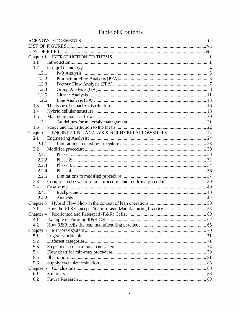
Table of Contents ACKNOWLEDGEMENTS........................................................................................................... iii LIST OF FIGURES ...................................................................................................................... vii LIST OF FILES ........................................................................................................................... viii Chapter 1 INTRODUCTION TO THESIS ................................................................................. 1
1.1 Introduction..................................................................................................................... 1 1.2 Group Technology .......................................................................................................... 4
1.2.1 P-Q Analysis ........................................................................................................... 5 1.2.2 Production Flow Analysis (PFA)............................................................................ 6 1.2.3 Factory Flow Analysis (FFA) ................................................................................. 7 1.2.4 Group Analysis (GA).............................................................................................. 8 1.2.5 Cluster Analysis .................................................................................................... 11 1.2.6 Line Analysis (LA) ............................................................................................... 13
1.3 The issue of capacity distribution: ................................................................................ 16 1.4 Hybrid cellular structure: .............................................................................................. 18 1.5 Managing material flow:............................................................................................... 20
1.5.1 Guidelines for materials management .................................................................. 21 1.6 Scope and Contribution to the thesis ............................................................................ 22
Chapter 2 ENGINEERING ANALYSIS FOR HYBRID FLOWSHOPS................................. 24 2.1 Engineering Analysis: ................................................................................................... 24
2.1.1 Limitations to existing procedure ......................................................................... 28 2.2 Modified procedure....................................................................................................... 29
2.2.1 Phase 1: ................................................................................................................. 30 2.2.2 Phase 2: ................................................................................................................. 32 2.2.3 Phase 3: ................................................................................................................. 34 2.2.4 Phase 4: ................................................................................................................. 36 2.2.5 Limitations to modified procedure........................................................................ 37
2.3 Comparison between Irani’s procedure and modified procedure ................................. 39 2.4 Case study ..................................................................................................................... 40
2.4.1 Background........................................................................................................... 40 2.4.2 Analysis................................................................................................................. 42
Chapter 3 Hybrid Flow Shop in the context of lean operations ................................................ 50 3.1 How the HFS Concept Fits Into Lean Manufacturing Practice .................................... 53
Chapter 4 Reoriented and Reshaped (R&R) Cells .................................................................... 60 4.1 Example of Forming R&R Cells................................................................................... 62 4.2 How R&R cells fits lean manufacturing practice ......................................................... 65
Chapter 5 Min-Max system ....................................................................................................... 70 5.1 Logistics principle......................................................................................................... 71 5.2 Different categories....................................................................................................... 71 5.3 Steps to establish a min-max system ............................................................................ 74 5.4 Flow chart for min-max procedure ............................................................................... 79 5.5 Illustration..................................................................................................................... 81 5.6 Supply cycle determination........................................................................................... 85
Chapter 6 Conclusions............................................................................................................... 88 6.1 Summary ....................................................................................................................... 88 6.2 Future Research ............................................................................................................ 89
iv

REFERENCES: ............................................................................................................................ 90 VITA………………………………………………………………………………...…...............92
v
LIST OF TABLES
Table 1-1: Initial Part-Machine Matrix......................................................................................... 10 Table 1-2: Final Part-Machine Matrix .......................................................................................... 11 Table 1-3: Utilization Matrix ........................................................................................................ 13 Table 1-4: Product Families.......................................................................................................... 16 Table 2-1: Operation Sequences [11] ........................................................................................... 24 Table 2-2: Common Sub-Strings for a group of machines [11] ................................................... 25 Table 2-3: Merger Co-efficient Matrix [11] ................................................................................. 26 Table 2-4: Layout Modules [11] ................................................................................................... 27 Table 2-5: Operation Sequences in terms of modules [11]........................................................... 28 Table 2-6: Common Sub-Strings for a group of products ............................................................ 30 Table 2-7: Operation sequences expressed in terms of modules .................................................. 34 Table 2-8: From/To modules ........................................................................................................ 36 Table 2-9: Comparision ................................................................................................................ 40 Table 2-10: A list of common sub-strings for a group of products and its occurence frequency. 43Table 2-11: Operation sequences expressed in terms of modules ................................................ 46 Table 2-12: From/To chart for modules........................................................................................ 47 Table 5-1: Container dimensions for parts.................................................................................... 81 Table 5-2: Part numbers sorted for min-max system.................................................................... 83 Table 5-3: Part numbers categorized based on frequency ............................................................ 86
vi
LIST OF FIGURES
Figure 1-1: Pareto Analysis ............................................................................................................ 6 Figure 1-2: Factory flow analysis ................................................................................................... 8 Figure 1-3: Hierarchical clustering to form part families [8] ....................................................... 12 Figure 1-4: Line analysis .............................................................................................................. 15 Figure 2-1: Clusters using co-efficient matrix [11] ...................................................................... 27 Figure 3-1: Group of machines ..................................................................................................... 51 Figure 3-3: Facility layout showing modules with uni-directional flow [14]............................... 52 Figure 3-4: Illustrates material flow ............................................................................................. 55 Figure 3-6: Illustrates material flow between cells....................................................................... 57 Figure 3-7: CONWIP loops in a HFS layout ................................................................................ 58 Figure 3-8: Parallelism within modules........................................................................................ 59 Figure 4-1: Facility layout with R&R cells................................................................................... 61 Figure 4-2: Groups of machines formed in to different layouts ................................................... 63 Figure 4-3: Cells reoriented and reshaped .................................................................................... 64 Figure 4-4: Similar machines co-located ...................................................................................... 64 Figure 4-5: First and last machines co-located ............................................................................. 66 Figure 4-6: Machine 'N2' capacity utilized by two adjacent cells ................................................ 67 Figure 5-1: Supply cycle frequency.............................................................................................. 71 Figure 5-2: Possible routes for a given group of products............................................................ 72 Figure 5-3: Flow rack with small containers ................................................................................ 74 Figure 5-4: Guidelines for supply cycle determination ................................................................ 76 Figure 5-6: Carts loaded with containers based on supply cycles ................................................ 78 Figure 5-7: Supply cycle for the current example ........................................................................ 85
vii

LIST OF FILES
NAME TYPE SIZE mohanmfs.pdf PDF 2.6 MB
viii
Chapter 1 INTRODUCTION TO THESIS
1.1 Introduction
The objective of lean manufacturing is to provide value to its customers by having a production
system whose structure and operations evolve towards the elimination of waste, leading to the
delivery of higher quality products at lower cost in a timely manner. In a highly competitive,
global market where niche product differentiation is short lived; organizations should primarily
focus on enhancing the production system. The capabilities required for successful performance
are generated and maintained through continuous improvements focusing on the perfection of the
lean system. According to Womack and Jones [1], to attain perfection we should first define
value from the customer’s eyes, do a value stream analysis, restructure the production system,
focus on continuous flow and link production stages through pull systems.
Value delivered to the customer is a key measure of the effectiveness of the production system.
According to Yingling [2], value is defined as the ratio of worth of outputs to cost of inputs.
Worth is the degree of satisfaction and utility the product gives to the customer. A production
system where the worth of the product produced is high and cost of inputs is low is considered to
be highly effective. Worth of the product is defined in terms of functionality, quality and
delivery of the product. Functionality looks at what the product has to offer in terms of
performance, features and aesthetics. Quality of a product is measured in terms of how well the
product meets the functionality targets over its lifecycle. Manufacturing conformance, reliability,
durability and maintainability are used as measures of quality. Delivery is how quickly the
product can be provided to the customer upon his/her request.
1
The system as a whole can be decomposed and viewed as a value stream through which the
product flows. Value streams consist of all tasks, material flows, and information flows used to
make the product. The components that form the product and the activities that are used to make
the product may be assessed individually in terms of the contribution to the value to the
customer. An activity that does not enhance (or may detract) from functionality, quality and
delivery is non-value added and should be eliminated if possible or at least the cost of that
activity should be reduced.
A pull system helps to produce to demand by providing the right part at the right quantity at the
right time with minimum inventory. It caps Work-In-Progress and keeps the inventory status
visible. Job dispatching decisions at processes are cognizant of floor status on downstream
routing, enabling dramatic reductions in the WIP levels necessary to maintain capacity of the
production system. Upon maturity, when low WIP caps are in place, pull also helps to increase
process coupling, thereby making problems on the floor immediately visible and urgent to
resolve. A pull system gives strong information feedback on the floor status. With
complementary management systems and human resource systems focused on problem
resolution, pull helps in the identification of the root cause for a problem and counter measures
can be taken to avoid it. Pull systems are primarily used to interlink production stages where one
has established flow.
According to Suzaki [3], flow is defined as “progressive movement of a product through a
facility from the receiving of raw materials to the shipping of finished product without stoppages
at any point in time due to backflows, machine breakdowns, or other production delays”.
2
Factories often have a functional organization with each department processing a particular step
in finished product. Raw material and WIP are routed through the departments to get the finished
product. The inefficiency of such a layout is due to:
• large travel distances in the material flow pattern
• large inter-machine transfer batch size
• high WIP levels as required by queuing of jobs at the processes
• large throughput times
• inefficient communication between the work centers that contributes to congestion in
product flow and delays in feedback when quality issues arise
• poor operations control because decoupling reduces urgency for problem resolution
• inefficient methodologies because processes lack focus on the needs of particular product
families and fail to consider waste that occurs in interfacing process steps
• reduced labor utilization due to “machine watching”
To overcome the inefficiencies and to get the benefits of lean manufacturing we should attain
flow first.
According to Tompkins et al [4], the three principles for effective flow planning within a facility
are 1) minimize flow, 2) maximize directed flow path, and 3) minimize cost of flow.
3
We try to minimize flow by:
• combining a few operations and
• eliminate those that do not add value to the part. (e.g.; sand blasting used to remove
oxidation because part flow is delayed)
We try to maximize directed flow path by:
• eliminating backtracking and
• avoiding cross flows between machines or lines dedicated to product families to the
maximum possible extent.
We try to minimize cost of flows by:
• eliminating handling.
• minimizing handling costs through use of efficient methods, and
• minimizing transportation delays.
By designing a facility based on the principles defined above, we attain attendant benefits in
throughput time, WIP inventory levels, and cost of manufacturing. Hence lean manufacturing
starts with flow and to realize the benefits of lean the facility should have flow.
1.2 Group Technology
According to Gallagher and Knight [5], group technology is a concept that identifies and brings
together related or similar parts and processes. A group technology cell can be defined as a cell
where a machine group is dedicated to a part family, Yingling [2]. Ideally, this cell would
4
process the parts through all steps in their routing. Groups of machines chosen for each product
family are situated together in a group layout. By reducing the number of stages of production
and avoiding cross flows, production control is enhanced. In turn this benefits throughput times,
WIP levels, quality, and cost of manufacturing. Inside the cell labor utilization increases because
workers operate on multiple processes. Moreover, specialized production methodologies can be
developed because of the manufacturing focus. This reduces labor requirements and enhances
quality. We now briefly review tools and procedures that may be used in group technology cell
formation.
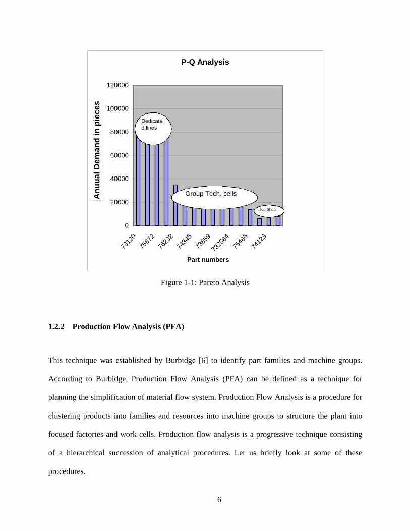
1.2.1 P-Q Analysis
P-Q analysis gives an insight on the type of facility appropriate for different products. A Pareto
chart is drawn by taking the part volumes and part numbers. This graph gives an idea on the type
of facility appropriate for the product. The graph shows how part volumes are related to the
dedicated lines, GT cells and job shops.
5
P-Q Analysis
0
20000
40000
60000
80000
100000
120000
7312
075
672
7623
274
345
7365
9
7325
8475
486
7412
3
Part numbers
Anu
ual D
eman
d in
pie
ces
Dedicated lines
Group Tech. cells
Job Shop
Figure 1-1: Pareto Analysis
1.2.2 Production Flow Analysis (PFA)
This technique was established by Burbidge [6] to identify part families and machine groups.
According to Burbidge, Production Flow Analysis (PFA) can be defined as a technique for
planning the simplification of material flow system. Production Flow Analysis is a procedure for
clustering products into families and resources into machine groups to structure the plant into
focused factories and work cells. Production flow analysis is a progressive technique consisting
of a hierarchical succession of analytical procedures. Let us briefly look at some of these
procedures.
6
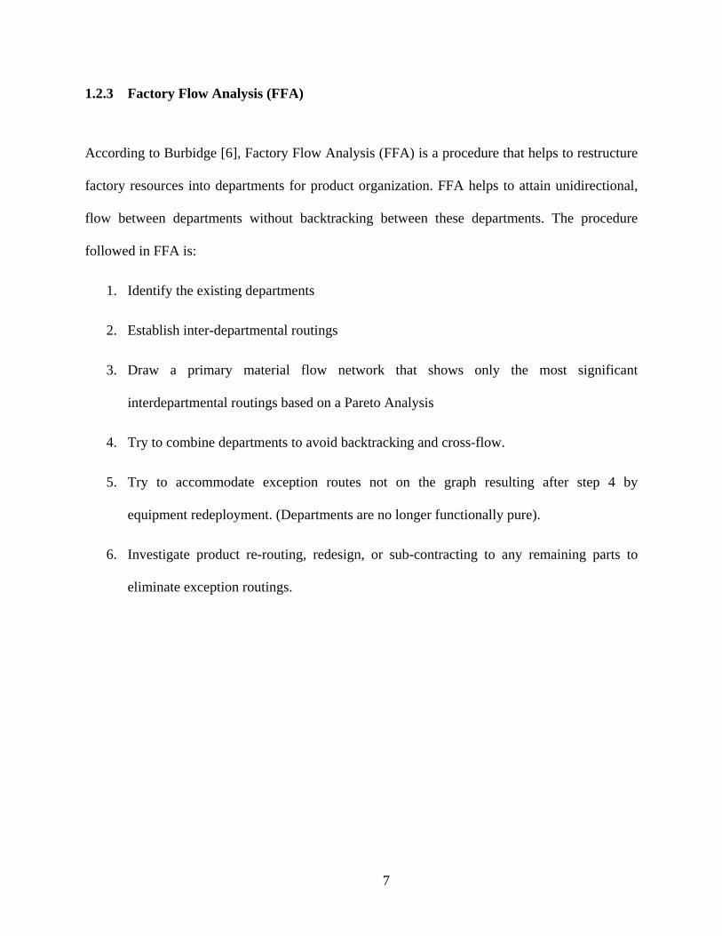
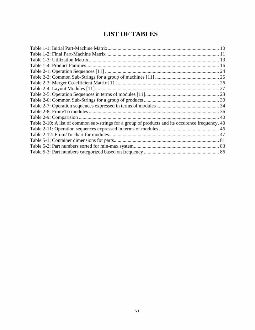
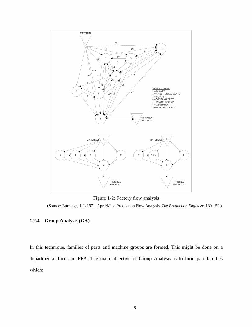
1.2.3 Factory Flow Analysis (FFA)
According to Burbidge [6], Factory Flow Analysis (FFA) is a procedure that helps to restructure
factory resources into departments for product organization. FFA helps to attain unidirectional,
flow between departments without backtracking between these departments. The procedure
followed in FFA is:
1. Identify the existing departments
2. Establish inter-departmental routings
3. Draw a primary material flow network that shows only the most significant
interdepartmental routings based on a Pareto Analysis
4. Try to combine departments to avoid backtracking and cross-flow.
5. Try to accommodate exception routes not on the graph resulting after step 4 by
equipment redeployment. (Departments are no longer functionally pure).
6. Investigate product re-routing, redesign, or sub-contracting to any remaining parts to
eliminate exception routings.
7
MATERIAL
1
2
3
4
5
6
9
1
1
3
3
2
84
126
151
53
15
28
161
3
1
1
3
1
1
45
12
8
1 26
27
FINISHEDPRODUCT
324
1
27
DEPARTMENTS1 = BLANKS2 = SHEET METAL WORK3 = FORGE4 = WELDING DEPT5 = MACHINE SHOP6 = ASSEMBLY9 = OUTSIDE FIRMS
1
6
2345
MATERIALS
FINISHEDPRODUCT
1
6
23 & 45
MATERIALS
FINISHEDPRODUCT
Figure 1-2: Factory flow analysis
(Source: Burbidge, J. L.1971, April/May. Production Flow Analysis. The Production Engineer, 139-152.)
1.2.4 Group Analysis (GA)
In this technique, families of parts and machine groups are formed. This might be done on a
departmental focus on FFA. The main objective of Group Analysis is to form part families
which:
8
• complete all the processing steps within the group technology cell
• Are provided with the necessary equipment to make them.
• Use the existing plant, without the need to purchase new machines.
• Use the existing processing methods with minor changes.
Key machine strategy: According to Burbidge [6], machines used in the factory floor can be
divided into five categories. They are:
1. Special – special operations can be performed on this machine only. Often times
there will be only one such machine on the floor.
2. Intermediate- same as S, but more than one machine exists
3. Common- several duplicate machines exist. e.g.; lathe, mill, and drill.
4. General- limited number of machines on floor, high capacity machines e.g.; paint
booth. These machines because of their nature (size, large volume of parts) are
difficult to integrate into cells
5. Equipment- inexpensive operations. Easy to duplicate. E.g. deburring machine.
SICGE classification helps to rank machines. G and E class machines are omitted from group
analysis (G class machines form service centers and E class machines are inexpensive and can be
easily duplicated).
A basic technique for group analysis called Rank Order Clustering (ROC) [7] is the resolution of
a binary incidence matrix. In this technique the parts and machines are represented by a binary
matrix. Table 1-1 illustrates this matrix for a real case where the company was manufacturing
hydraulic brake systems used in the automotive industry and the company was implementing
9
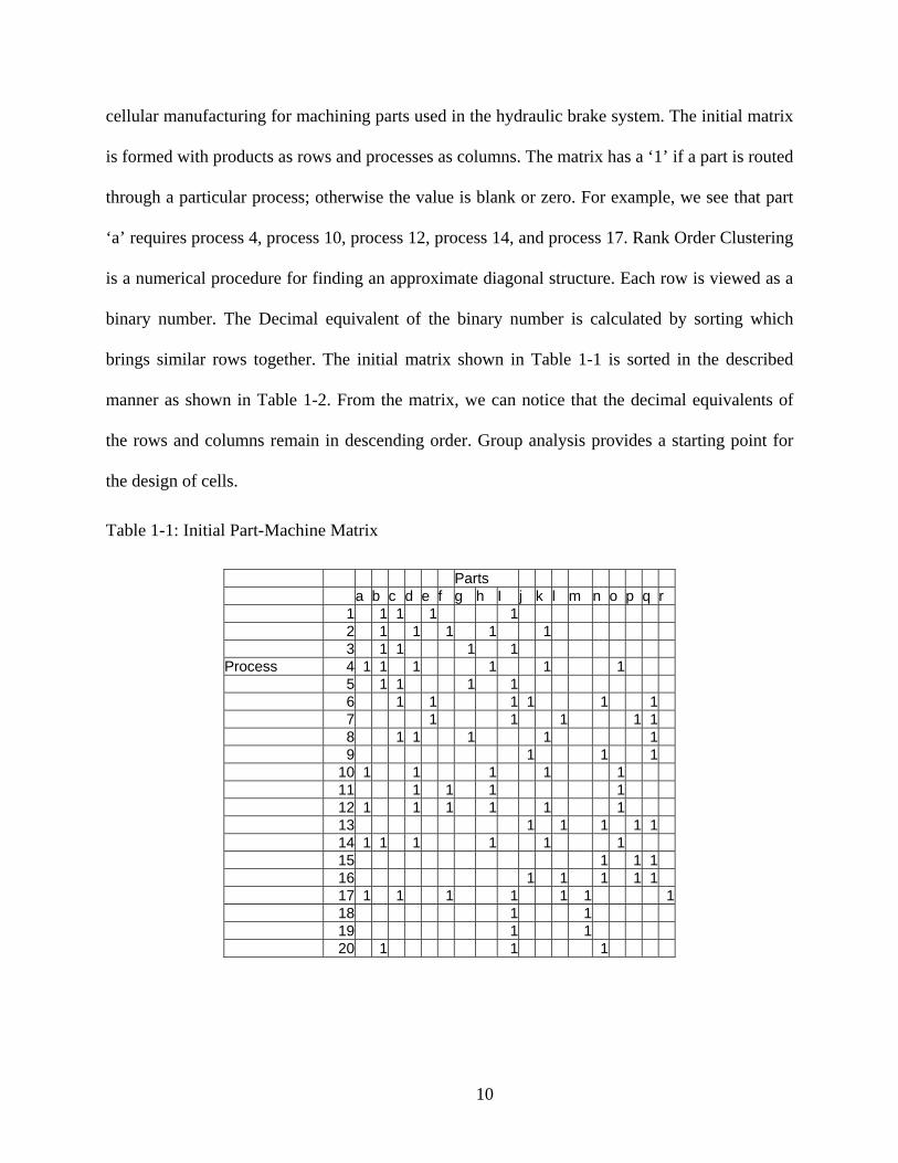
cellular manufacturing for machining parts used in the hydraulic brake system. The initial matrix
is formed with products as rows and processes as columns. The matrix has a ‘1’ if a part is routed
through a particular process; otherwise the value is blank or zero. For example, we see that part
‘a’ requires process 4, process 10, process 12, process 14, and process 17. Rank Order Clustering
is a numerical procedure for finding an approximate diagonal structure. Each row is viewed as a
binary number. The Decimal equivalent of the binary number is calculated by sorting which
brings similar rows together. The initial matrix shown in Table 1-1 is sorted in the described
manner as shown in Table 1-2. From the matrix, we can notice that the decimal equivalents of
the rows and columns remain in descending order. Group analysis provides a starting point for
the design of cells.
Table 1-1: Initial Part-Machine Matrix
Parts a b c d e f g h I j k l m n o p q r 1 1 1 1 1 2 1 1 1 1 1 3 1 1 1 1 Process 4 1 1 1 1 1 1 5 1 1 1 1 6 1 1 1 1 1 1 7 1 1 1 1 1 8 1 1 1 1 1 9 1 1 1 10 1 1 1 1 1 11 1 1 1 1 12 1 1 1 1 1 1 13 1 1 1 1 1 14 1 1 1 1 1 1 15 1 1 1 16 1 1 1 1 1 17 1 1 1 1 1 1 1 18 1 1 19 1 1 20 1 1 1
10
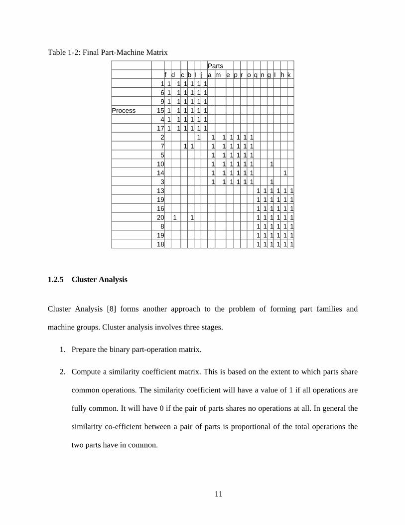
Table 1-2: Final Part-Machine Matrix
Parts f d c b I j a m e p r o q n g I h k 1 1 1 1 1 1 1 6 1 1 1 1 1 1 9 1 1 1 1 1 1 Process 15 1 1 1 1 1 1 4 1 1 1 1 1 1 17 1 1 1 1 1 1 2 1 1 1 1 1 1 1 7 1 1 1 1 1 1 1 1 5 1 1 1 1 1 1 10 1 1 1 1 1 1 1 14 1 1 1 1 1 1 1 3 1 1 1 1 1 1 1 13 1 1 1 1 1 1 19 1 1 1 1 1 1 16 1 1 1 1 1 1 20 1 1 1 1 1 1 1 1 8 1 1 1 1 1 1 19 1 1 1 1 1 1 18 1 1 1 1 1 1
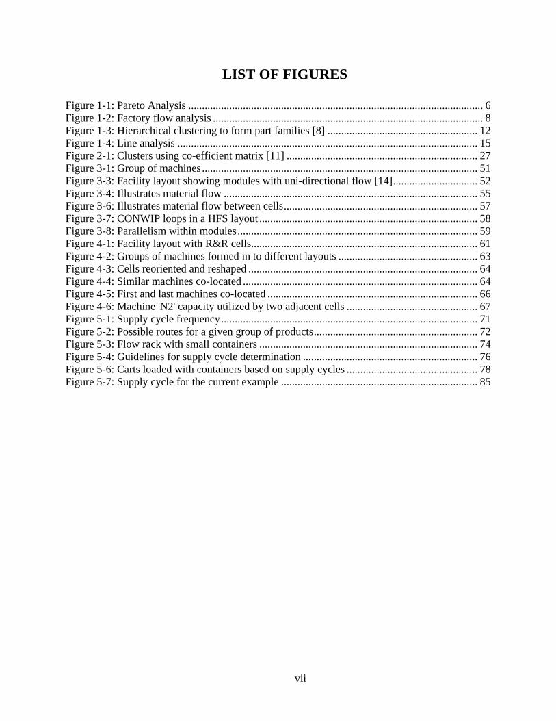
1.2.5 Cluster Analysis Cluster Analysis [8] forms another approach to the problem of forming part families and
machine groups. Cluster analysis involves three stages.
1. Prepare the binary part-operation matrix.
2. Compute a similarity coefficient matrix. This is based on the extent to which parts share
common operations. The similarity coefficient will have a value of 1 if all operations are
fully common. It will have 0 if the pair of parts shares no operations at all. In general the
similarity co-efficient between a pair of parts is proportional of the total operations the
two parts have in common.
11
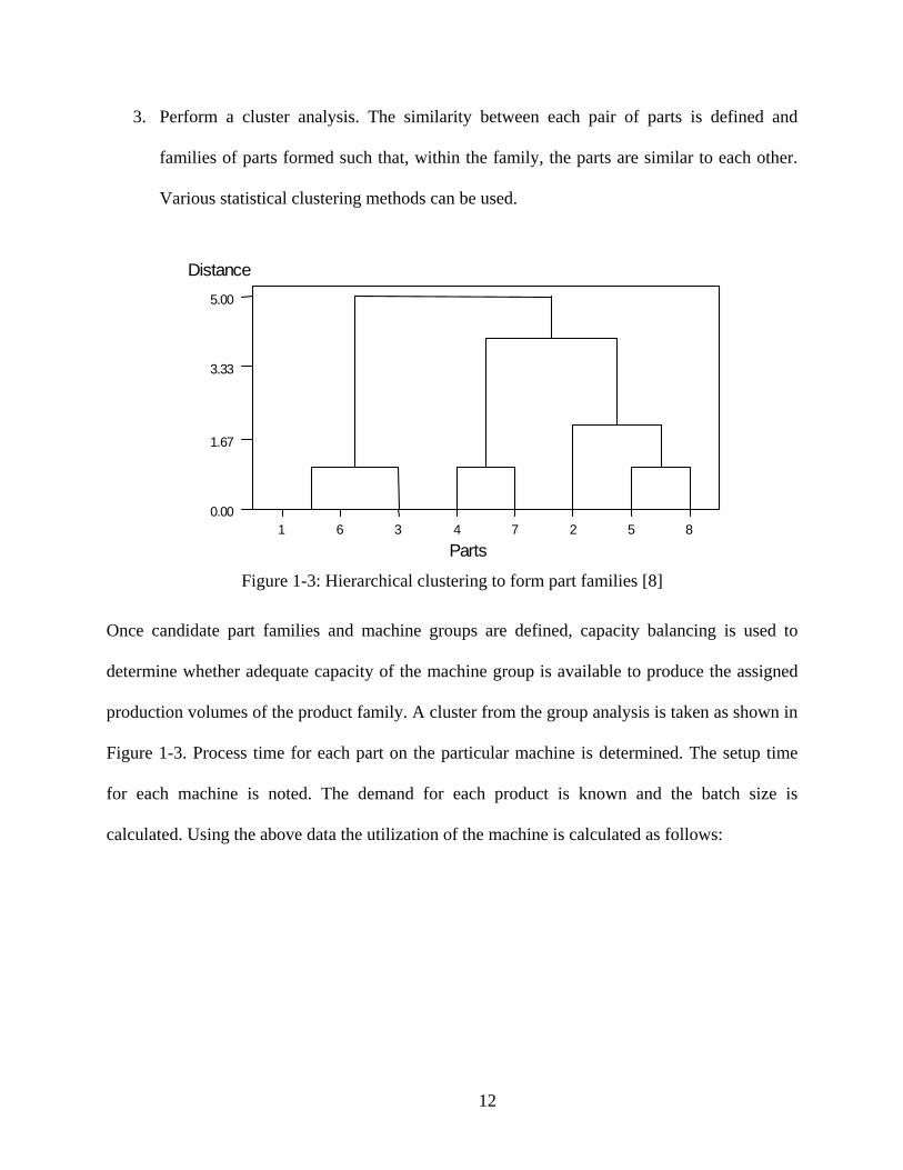
3. Perform a cluster analysis. The similarity between each pair of parts is defined and
families of parts formed such that, within the family, the parts are similar to each other.
Various statistical clustering methods can be used.
1 6 3 4 7 2 5 80.00
1.67
3.33
5.00
Parts
Distance
Figure 1-3: Hierarchical clustering to form part families [8]
Once candidate part families and machine groups are defined, capacity balancing is used to
determine whether adequate capacity of the machine group is available to produce the assigned
production volumes of the product family. A cluster from the group analysis is taken as shown in
Figure 1-3. Process time for each part on the particular machine is determined. The setup time
for each machine is noted. The demand for each product is known and the batch size is
calculated. Using the above data the utilization of the machine is calculated as follows:
12
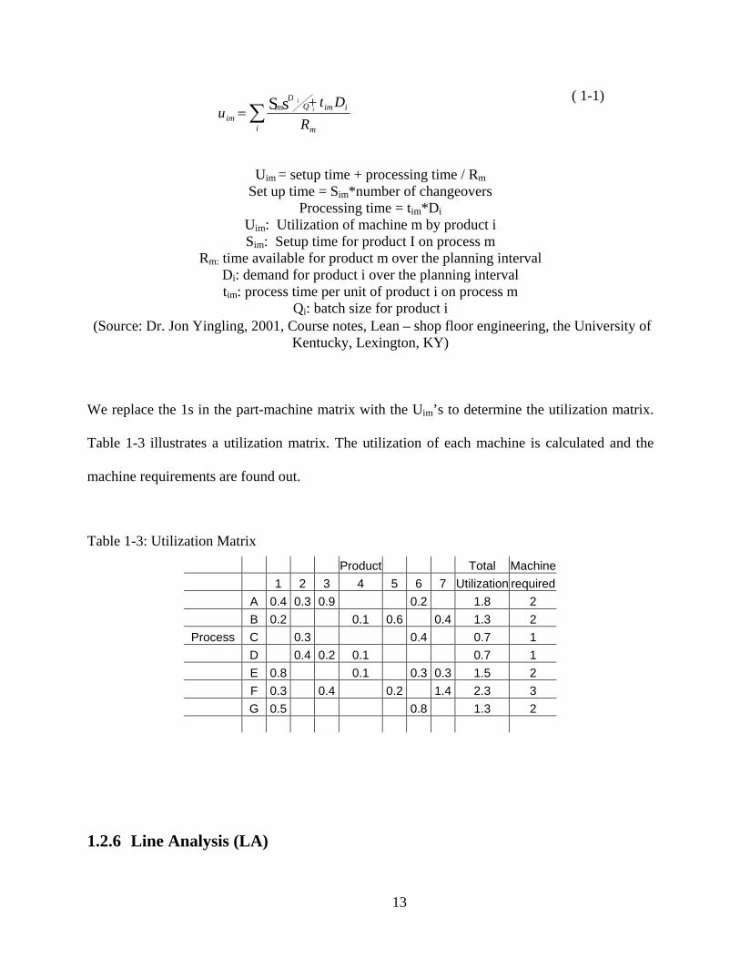
( 1-1)
Uim = setup time + processing time / Rm
Set up time = Sim*number of changeovers Processing time = tim*Di
Uim: Utilization of machine m by product i Sim: Setup time for product I on process m
Rm: time available for product m over the planning interval Di: demand for product i over the planning interval tim: process time per unit of product i on process m
Qi: batch size for product i (Source: Dr. Jon Yingling, 2001, Course notes, Lean – shop floor engineering, the University of
Kentucky, Lexington, KY) We replace the 1s in the part-machine matrix with the Uim’s to determine the utilization matrix.
Table 1-3 illustrates a utilization matrix. The utilization of each machine is calculated and the
machine requirements are found out.
Table 1-3: Utilization Matrix
Product Total Machine 1 2 3 4 5 6 7 Utilization required A 0.4 0.3 0.9 0.2 1.8 2 B 0.2 0.1 0.6 0.4 1.3 2
Process C 0.3 0.4 0.7 1 D 0.4 0.2 0.1 0.7 1 E 0.8 0.1 0.3 0.3 1.5 2 F 0.3 0.4 0.2 1.4 2.3 3 G 0.5 0.8 1.3 2
1.2.6 Line Analysis (LA)
∑
+=
i m
iimim im R
DtS s D iQu i
13
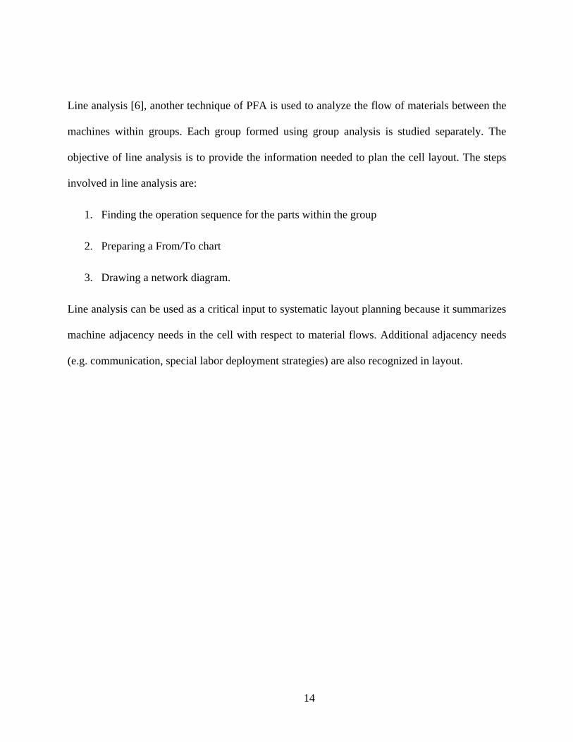
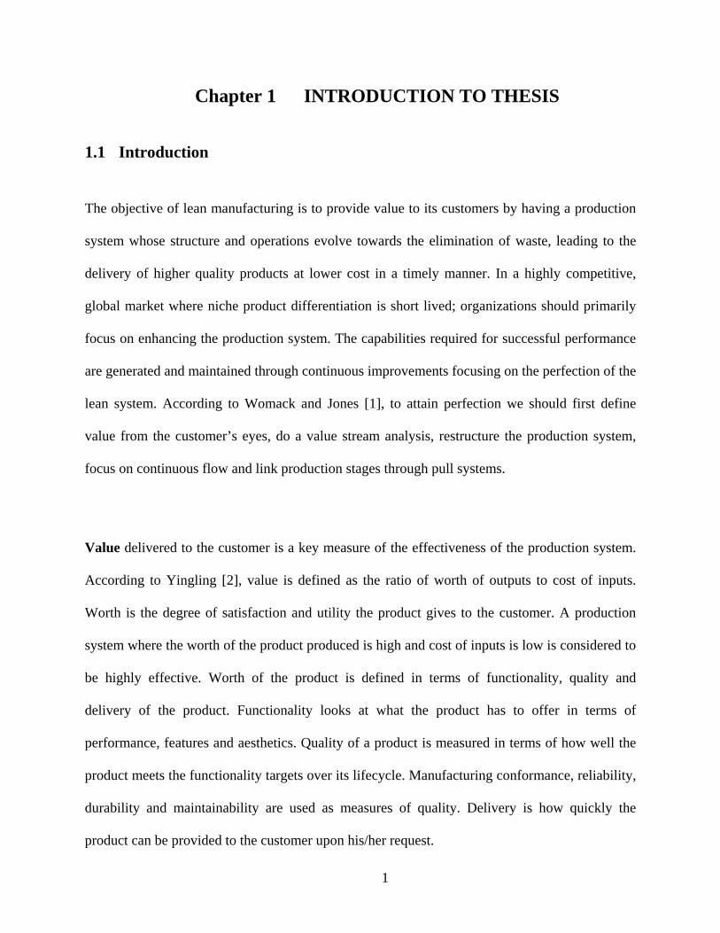
Line analysis [6], another technique of PFA is used to analyze the flow of materials between the
machines within groups. Each group formed using group analysis is studied separately. The
objective of line analysis is to provide the information needed to plan the cell layout. The steps
involved in line analysis are:
1. Finding the operation sequence for the parts within the group
2. Preparing a From/To chart
3. Drawing a network diagram.
Line analysis can be used as a critical input to systematic layout planning because it summarizes
machine adjacency needs in the cell with respect to material flows. Additional adjacency needs
(e.g. communication, special labor deployment strategies) are also recognized in layout.
14
MATERIAL
1HS4
2HS
3MO
4DS
5MV
8SA
65 17
611
1
2
3
111
3 2 4
41 2 5 4 4 16 2
2
GROUP FLOW NETWORK DIAGRAM - GROUP 2
SIMPLIFIED GROUP FLOW NETWORK - GROUP 2
8SA
4DH
6MH
7DS
5MV
MATERIALS
1HS4
72
42
72
17
15 85
2
2
1
1
4 3
1
6
7DH
6MH
Figure 1-4: Line analysis
(Source: Burbidge, J. L.1971, April/May. Production Flow Analysis. The Production Engineer, 139-152.)
15
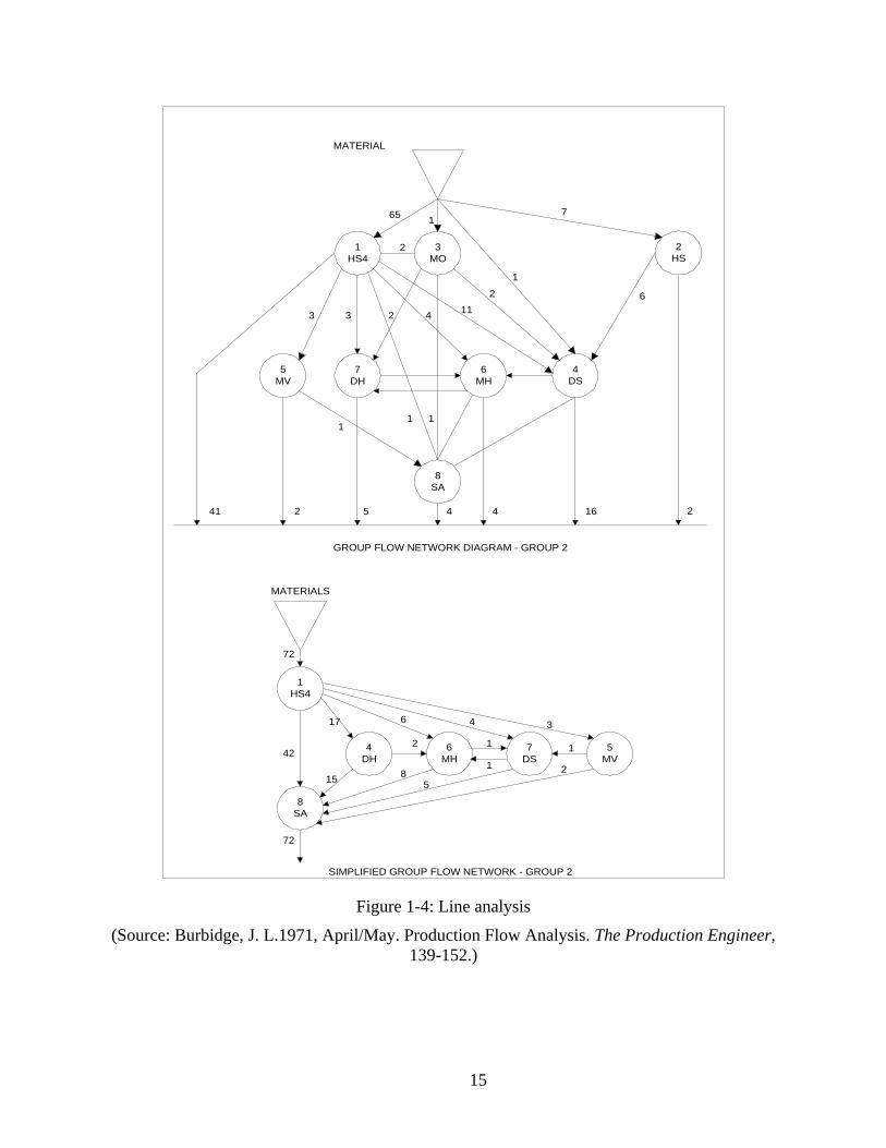
1.3 The issue of capacity distribution: Table 1-4: Product Families
L48267B
K34596
M48265D
E33494
K44276C
L48388M
E7392
K34098A
K45199
K43590
M61592
M48195C
M44276D
E34267
E12204
E18694
E41795
E48596
M48386H
K48251A
L48388
M45691D
M45691B
M44276E
K47697
E47782
E46364
E12288
E33295
E48586
M47693F
PG X X X X X X
DM 3/1 X X X X
DXY 3/1 X X
RP X GROUP-1
FAMILY – 1
P&G X X X X X X X X X X X X ONE “EXCEPTION” X
DMT 3/2 X X X X X X X
DM 3/2 X X X X X X
DXY 3/2 X X X X X X
W&P X X X X X X
WG3
X GROU
P-2
FAMILY - 2
PGG X X X
PGB X X X X X X
PGR X X
DMT 3/3 X X X X
DM 3/3 X X X
P&GR X
GROU
P-3
MACHINE/WORKSTATION
FAMILY –3
(Source: Burbidge, J. L.1971, Production Flow Analysis. The Production Engineer, 139-152)
Cellular manufacturing often suggests that machines be duplicated to maintain part family and
machine focus. Table 1.4 shows the clusters formed after applying a binary sorting procedure.
We could see from the figure that two part families require P&G. Ideally this machine type
would be duplicated and units would be distributed among the cells to maintain capability for
completing all operations of the part family in a single cell. However this might result in under
utilizing the machine. The capacity of the machine might go wasted. Hence the traditional cells
do not have the capacity flexibility.
16
Expensive single machines such as gear hobbers, cylindrical grinders, machining centers, etc.,
may not be practical to replicate among multiple cells. To keep their utilization high, companies
may prefer loading parts from several families on them. Intercell flows to such machines cannot
be eliminated. Similarly, incompatible processes such as treatment or presswork must normally
be excluded from the cells due to equipment costs, environmental problems, size, or
incompatibility with other processes.
However, by carefully locating and shaping cells it may be possible to efficiently share machines
between cells. For example, in the previous example assume that cluster 2 requires 0.3 units of
P&G and cluster 3 requires 0.4 units. Ideally 1 unit of P&G would be located in each cell.
Instead, by carefully orienting and reshaping the cells it may be possible to have 1 unit of P&G
shared between the cells. By reorienting and reshaping cells it may be possible to increase the
total processing time on machine m thereby achieving higher utilization for machine m.
Tooling analysis helps to schedule the cell by identifying parts with similar setup requirements.
Tooling analysis may be used to refine parts families, identifying a set of parts where one can
rapidly change between the members of these sets. It may also be used to identify part number
sequences that reduce setup requirements by avoiding tooling changes between the parts in
sequence. Tooling analysis helps to increase the machine capacity on bottleneck machines.
Note that intracell layout and product sequencing through machines can influence machine
distribution decisions. For example, two part families may be using the same machine type.
From the flow perspective the machine might be deployed in different positions in the flow line
for each family. Parts in family 1 may require the machine either at the beginning or the end of
the operation sequences. Parts in family 2 might require the machine in the middle of their
operation sequence. Intracell layout design might assign the machine to family 2 to make the
17
intercell flow scheduling problem easy. Parts can be processed in cell 1 either before or after
they are processed in cell 2 but there is no need for cross flows between the cells.
Also note that in the case of instabilities such as machine breakdown the product flow gets
disrupted. The part has to be batched before the broken machine and taken to a replicate
machine, if it exists. This creates an out of cell flow. By keeping the key like machines close to
each other, the plant attains the much-needed flexibility to deal with such contingencies. By
having like machines close to each other, the intercell distance and intracell distance are almost
equal. In case of instabilities such as machine breakdowns and demand changes the part can be
routed to the adjacent like machine. This preserves the flow for the product and creates a more
robust manufacturing facility.
1.4 Hybrid cellular structure: In order to have part family focus it is desired that all of the machines required by the family be
placed within the cell. But because of the practical issues noted above, this does not mean that all
the machines required by the family can actually be located within the cell. According to Irani
[9], the cell formation problem can be broken into four sub problems.
The first sub problem is the identification of part families and machine groups. The traditional
approach has been to design cells to focus on a single family of product. This allows each
machine group to be matched with a suitable part family.
The second sub problem is the distribution of machines among the cells formed. The cells may
have common machine requirements if a) several part families require operation on the same
type of machine or, b) there is only one machine of the type that cannot be assigned to any
18
particular cell. If such cases exists, a compromise between the independence of the cells and
intercell flows should be made. Machine utilization must be considered while making a decision.
The third sub problem is that of intracell layout design. Within a cell, the machines are arranged
based on the overall sequence of operations. All the parts need not be visiting every machine in
the cell and can jump stations. Hence unidirectional material flow may not always be possible
and backtracking may exist. This can be accommodated by suitable handling system or perhaps
by duplicating machines.
The fourth sub problem is that of intercell layout. This problem arises when machines have to be
shared when there is only one machine of the type that cannot be assigned to any particular cell
or when product families should flow through multiple cells. For the first two requirements the
intercell layout should be designed so as to locate cells with common machine requirements
close to each other. This will facilitate intercell material handling. If product volumes routed
through multiple cells are high, those cells should also be located close to each other as well.
The traditional PFA cell formation approach focuses on part family formation and machine
distribution and neglects the layout design issues involving multiple part families and cells with
cross flows. In order to consider the sub problems together, several researchers have investigated
the utility of a hybrid cellular layout. This is simply a combination of functional and cellular
layouts. Having a functional layout for some shared machine types offers high machine
utilization and loading flexibility. By having part family focus the benefits of reduced throughput
times and handling costs are gained.
Hence a hybrid cellular structure relaxes the traditional view that a cell must be dedicated to a
single part family. Parts from a family may visit adjacent cells other than the cells they have been
assigned to.
19
By hybrid cellular structure we mean
1. Locating dedicated machines and their supporting equipment to single part families in
cells.
2. Locating non-dedicated shared machines close to each other as in functionally organized
sections accessible to all the cells if intercell flow between adjacent cells exists.
3. Designing an approximate layout within and between the cells to eliminate backtracking.
4. Designing the overall shop layout based on the overlapping machine requirements to
reduce intercell flows.
1.5 Managing material flow: Many facilities are creating single piece continuous flow processes but are backing them with
undependable material-delivery systems. In most facilities there is a central schedule (often in
the form of a material requirement planning system), it calls for materials to be delivered to
points of use in precise amounts at precise times, from receiving, a storage area or an upstream
activity. But the schedule is continually changing and many of the centralized instructions do not
reflect the floor realities. Due to this they lose production and incur extra-material handling
costs. The consequences are:
• Output varies due to part shortages and/or wrong parts being delivered to the cells.
• Operators carry the burden of searching for parts and performing material handling tasks.
• Extra cost due to excess inventory and parts being stored at different locations
• Increase in forklift miles due to parts being scattered in different locations around the
plant and unplanned, inefficient routing of vehicles in the delivery of parts to point of use
20
• Higher costs to expedite parts to support production.
Please note that even if the management believes in the need for a precise material handling
process, it’s not possible to get there incrementally with “point” kaizen fixing individual process
steps. Nor is it possible to get there with “flow” kaizen for a single product family‘s value
stream. What is needed is a “system” kaizen in which the material handling system for the entire
facility is redesigned to create a process that is precise and stable.
Such a system must include a plan for every part that documents all relevant information about
each part number in the facility, including its storage location and points of use. It must also
include a single storage location and minimum and maximum inventory quantities for both
purchased parts and for work-in-process. In addition, a material-handling system requires precise
delivery routes with standard work to get every part from its storage location to its point of use
exactly when needed.
1.5.1 Guidelines for materials management
According to Mike Rother and Rick Harris [10], the following are the guidelines for structuring a
materials management that would help your cell operators perform their work as efficiently as
possible.
1. Present parts as close as possible to the point of use, but not in the walking path of the
operator.
2. Present parts so that operator can use both hands simultaneously.
21
3. Do not have operators get or restock their own parts.
4. Do not put additional parts storage in or near the process because this makes the
operation of the cell harder to understand and encourages the operators to get their own
parts.
5. Utilize proper materials management system to regulate parts replenishment.
6. Size parts container for the convenience of the operators or as a multiple of finished
goods pack quantity.
7. Do not interrupt operator work cycles to replenish parts.
1.6 Scope and Contribution to the thesis
1. Hybrid Cellular Constructs, which, to date, have only been described as general concepts
in the literature, specifically Hybrid Flow Shops and Reoriented and Reshaped Cells are
clearly described in terms of their structure, key features, and modes of operation in
complex industrial environments (e.g. high variety, low volume, non-repetitive
manufacturing).
2. The presentation explains each structure and discusses an engineering procedure for
defining the structures.
3. Particular manufacturing circumstances where each concept would be most useful. The
engineering procedure is illustrated by cases.
22
4. This thesis then defines lean practices that are compatible with the cell type in question
and identifies what practices are incompatible. It suggests how to modify lean practices
and at least obtain some benefits for the incompatible ones.
5. A procedure for design of hybrid cellular constructs which the author assisted in
development (Narayanan, M. (2002), Hybrid Flow Strategies for high variety low volume
manufacturing facilities to implement flow and pull, Masters of Science thesis,
department of Manufacturing Systems Engineering, the University of Kentucky,
Lexington, KY) is described as an engineering design approach for that type of system.
6. A procedure for design of logistics management systems for assembly cells and lines has
been developed and described herein.
Copyright © Mohan Swaminathan 2004
23
Chapter 2 ENGINEERING ANALYSIS FOR HYBRID
FLOWSHOPS
2.1 Engineering Analysis: Irani et al [11] have proposed a heuristic method for forming layouts in the form of layout
modules. According to Irani et al [11], layout modules automatically group machines that occur
together in different operation sequences, allowing the same machines to be duplicated in several
locations, depending on the placement of the layout modules in the final layout.
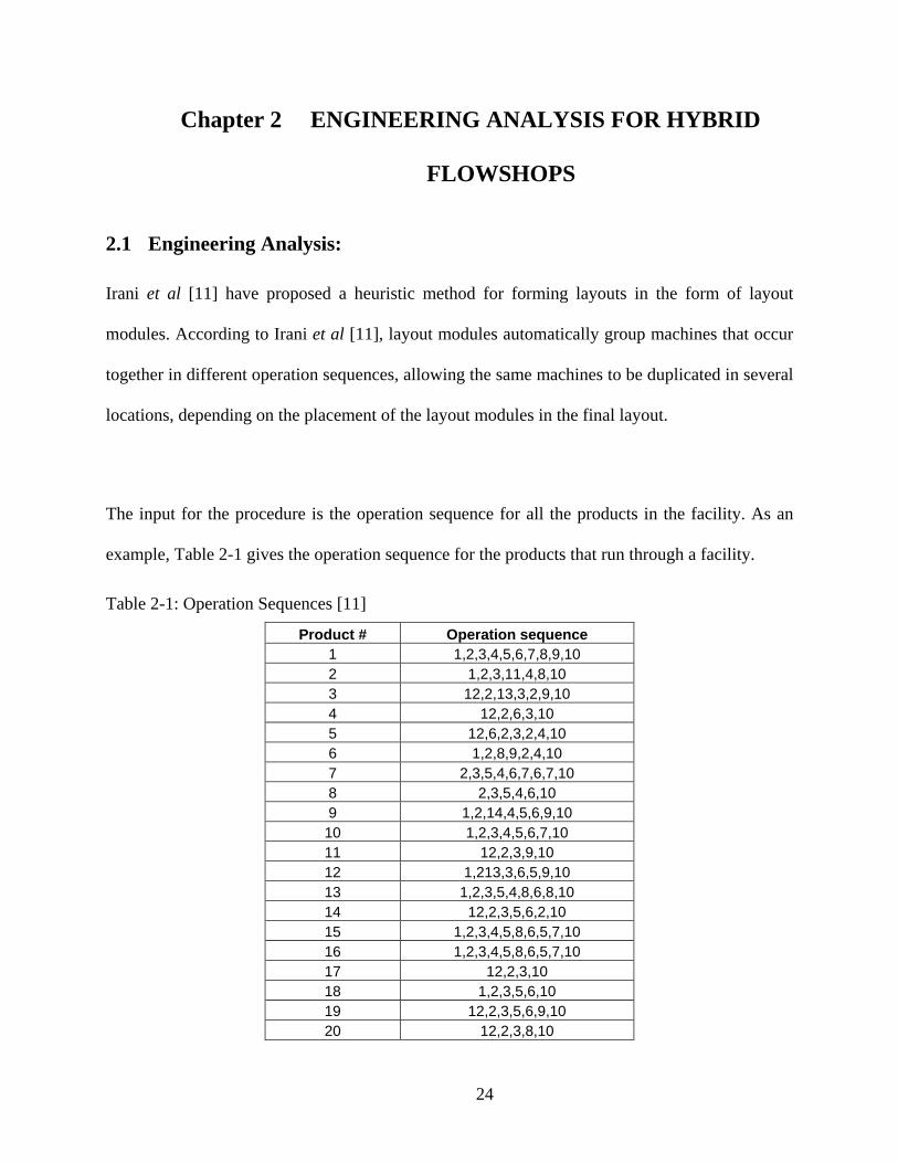
The input for the procedure is the operation sequence for all the products in the facility. As an
example, Table 2-1 gives the operation sequence for the products that run through a facility.
Table 2-1: Operation Sequences [11]
Product # Operation sequence 1 1,2,3,4,5,6,7,8,9,10 2 1,2,3,11,4,8,10 3 12,2,13,3,2,9,10 4 12,2,6,3,10 5 12,6,2,3,2,4,10 6 1,2,8,9,2,4,10 7 2,3,5,4,6,7,6,7,10 8 2,3,5,4,6,10 9 1,2,14,4,5,6,9,10 10 1,2,3,4,5,6,7,10 11 12,2,3,9,10 12 1,213,3,6,5,9,10 13 1,2,3,5,4,8,6,8,10 14 12,2,3,5,6,2,10 15 1,2,3,4,5,8,6,5,7,10 16 1,2,3,4,5,8,6,5,7,10 17 12,2,3,10 18 1,2,3,5,6,10 19 12,2,3,5,6,9,10 20 12,2,3,8,10
24
21 1,2,3,4,5,6,7,5,10 22 1,2,5,6,4,9,10 23 12,2,10 24 12,2,3,10 25 12,2,3,5,4,6,9,10
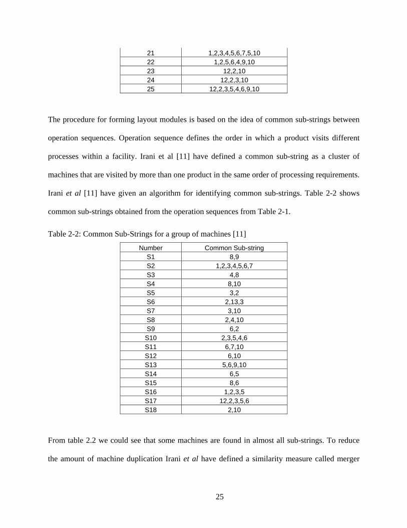
The procedure for forming layout modules is based on the idea of common sub-strings between
operation sequences. Operation sequence defines the order in which a product visits different
processes within a facility. Irani et al [11] have defined a common sub-string as a cluster of
machines that are visited by more than one product in the same order of processing requirements.
Irani et al [11] have given an algorithm for identifying common sub-strings. Table 2-2 shows
common sub-strings obtained from the operation sequences from Table 2-1.
Table 2-2: Common Sub-Strings for a group of machines [11]
Number Common Sub-string S1 8,9 S2 1,2,3,4,5,6,7 S3 4,8 S4 8,10 S5 3,2 S6 2,13,3 S7 3,10 S8 2,4,10 S9 6,2
S10 2,3,5,4,6 S11 6,7,10 S12 6,10 S13 5,6,9,10 S14 6,5 S15 8,6 S16 1,2,3,5 S17 12,2,3,5,6 S18 2,10
From table 2.2 we could see that some machines are found in almost all sub-strings. To reduce
the amount of machine duplication Irani et al have defined a similarity measure called merger
25
coefficient that will identify similar common sub-strings. The larger the merger co-efficient the
more similar the sub-strings are. Like similarity co-efficients, merger co-efficient vary between 0
and 1. For a detailed procedure on how to calculate merger co-efficient please refer to Irani et al
[11].
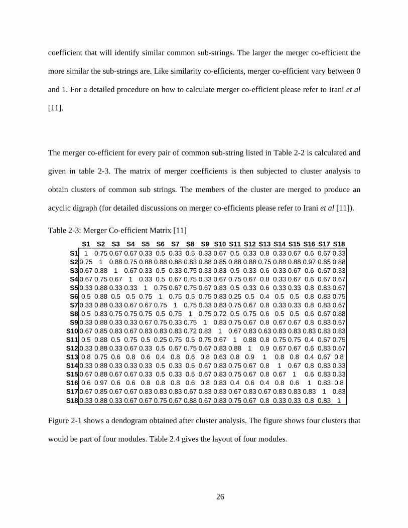
The merger co-efficient for every pair of common sub-string listed in Table 2-2 is calculated and
given in table 2-3. The matrix of merger coefficients is then subjected to cluster analysis to
obtain clusters of common sub strings. The members of the cluster are merged to produce an
acyclic digraph (for detailed discussions on merger co-efficients please refer to Irani et al [11]).
Table 2-3: Merger Co-efficient Matrix [11]
S1 S2 S3 S4 S5 S6 S7 S8 S9 S10 S11 S12 S13 S14 S15 S16 S17 S181 0.75 0.67 0.67 0.33 0.5 0.33 0.5 0.33 0.67 0.5 0.33 0.8 0.33 0.67 0.6 0.67 0.33S1
S2 0.75 1 0.88 0.75 0.88 0.88 0.88 0.83 0.88 0.85 0.88 0.88 0.75 0.88 0.88 0.97 0.85 0.88S3 0.67 0.88 1 0.67 0.33 0.5 0.33 0.75 0.33 0.83 0.5 0.33 0.6 0.33 0.67 0.6 0.67 0.33S4 0.67 0.75 0.67 1 0.33 0.5 0.67 0.75 0.33 0.67 0.75 0.67 0.8 0.33 0.67 0.6 0.67 0.67S5 0.33 0.88 0.33 0.33 1 0.75 0.67 0.75 0.67 0.83 0.5 0.33 0.6 0.33 0.33 0.8 0.83 0.67
0.5 0.88 0.5 0.5 0.75 1 0.75 0.5 0.75 0.83 0.25 0.5 0.4 0.5 0.5 0.8 0.83 0.75S6 S7 0.33 0.88 0.33 0.67 0.67 0.75 1 0.75 0.33 0.83 0.75 0.67 0.8 0.33 0.33 0.8 0.83 0.67S8 0.5 0.83 0.75 0.75 0.75 0.5 0.75 1 0.75 0.72 0.5 0.75 0.6 0.5 0.5 0.6 0.67 0.88S9 0.33 0.88 0.33 0.33 0.67 0.75 0.33 0.75 1 0.83 0.75 0.67 0.8 0.67 0.67 0.8 0.83 0.67
S10 0.67 0.85 0.83 0.67 0.83 0.83 0.83 0.72 0.83 1 0.67 0.83 0.63 0.83 0.83 0.83 0.83 0.83S11 0.5 0.88 0.5 0.75 0.5 0.25 0.75 0.5 0.75 0.67 1 0.88 0.8 0.75 0.75 0.4 0.67 0.75S12 0.33 0.88 0.33 0.67 0.33 0.5 0.67 0.75 0.67 0.83 0.88 1 0.9 0.67 0.67 0.6 0.83 0.67
0.8 0.75 0.6 0.8 0.6 0.4 0.8 0.6 0.8 0.63 0.8 0.9 1 0.8 0.8 0.4 S13 0.67 0.8S14 0.33 0.88 0.33 0.33 0.33 0.5 0.33 0.5 0.67 0.83 0.75 0.67 0.8 1 0.67 0.8 0.83 0.33S15 0.67 0.88 0.67 0.67 0.33 0.5 0.33 0.5 0.67 0.83 0.75 0.67 0.8 0.67 1 0.6 0.83 0.33S16 0.6 0.97 0.6 0.6 0.8 0.8 0.8 0.6 0.8 0.83 0.4 0.6 0.4 0.8 0.6 1 0.83 0.8S17 0.67 0.85 0.67 0.67 0.83 0.83 0.83 0.67 0.83 0.83 0.67 0.83 0.67 0.83 0.83 0.83 1 0.83S18 0.33 0.88 0.33 0.67 0.67 0.75 0.67 0.88 0.67 0.83 0.75 0.67 0.8 0.33 0.33 0.8 0.83 1
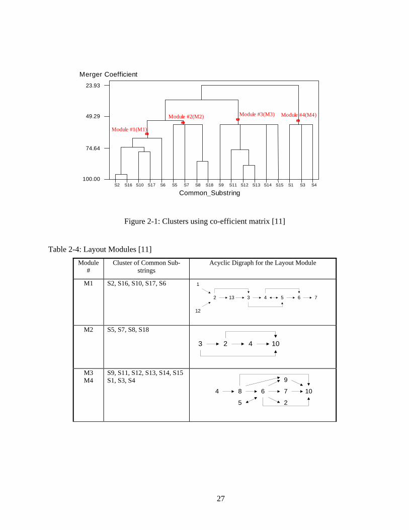
Figure 2-1 shows a dendogram obtained after cluster analysis. The figure shows four clusters that
would be part of four modules. Table 2.4 gives the layout of four modules.
26
S 2 S 1 6 S 1 0 S 1 7 S 6 S5 S7 S8 S18 S9 S11 S12 S13 S14 S15 S 1 S 3 S 4 1 0 0 . 0 0
7 4 . 6 4
4 9 . 2 9
2 3 . 9 3
Common_Substring
M e r g e r C o e f f ic i e n t
M o d u l e # 1 ( M 1 )
Module #2(M2) Module #3(M3) Mo d u l e # 4 ( M 4 )
Figure 2-1: Clusters using co-efficient matrix [11]
Table 2-4: Layout Modules [11]
Module #
Cluster of Common Sub-strings
Acyclic Digraph for the Layout Module
M1 S2, S16, S10, S17, S6
2 13 3 4 5 6 7
1
12
M2 S5, S7, S8, S18
3 2 4 10
M3 M4
S9, S11, S12, S13, S14, S15 S1, S3, S4
4 8 6 7 10
9
25
27
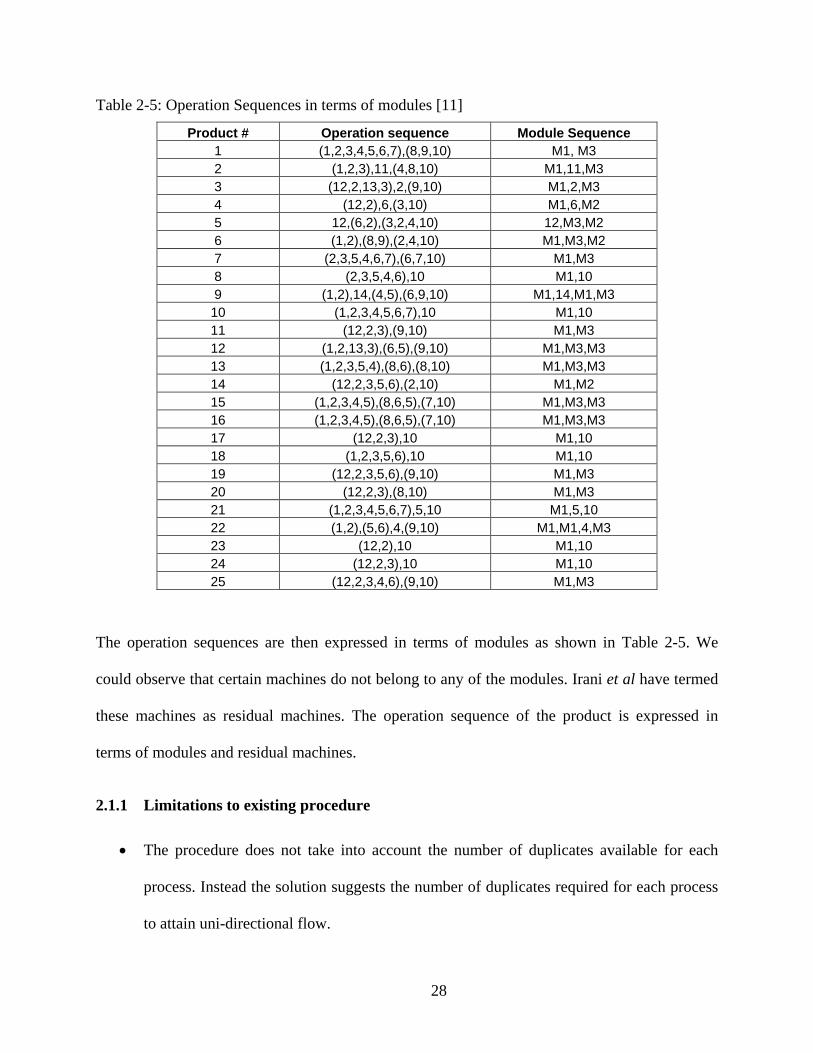
Table 2-5: Operation Sequences in terms of modules [11]
Product # Operation sequence Module Sequence 1 (1,2,3,4,5,6,7),(8,9,10) M1, M3 2 (1,2,3),11,(4,8,10) M1,11,M3 3 (12,2,13,3),2,(9,10) M1,2,M3 4 (12,2),6,(3,10) M1,6,M2 5 12,(6,2),(3,2,4,10) 12,M3,M2 6 (1,2),(8,9),(2,4,10) M1,M3,M2 7 (2,3,5,4,6,7),(6,7,10) M1,M3 8 (2,3,5,4,6),10 M1,10 9 (1,2),14,(4,5),(6,9,10) M1,14,M1,M3 10 (1,2,3,4,5,6,7),10 M1,10 11 (12,2,3),(9,10) M1,M3 12 (1,2,13,3),(6,5),(9,10) M1,M3,M3 13 (1,2,3,5,4),(8,6),(8,10) M1,M3,M3 14 (12,2,3,5,6),(2,10) M1,M2 15 (1,2,3,4,5),(8,6,5),(7,10) M1,M3,M3 16 (1,2,3,4,5),(8,6,5),(7,10) M1,M3,M3 17 (12,2,3),10 M1,10 18 (1,2,3,5,6),10 M1,10 19 (12,2,3,5,6),(9,10) M1,M3 20 (12,2,3),(8,10) M1,M3 21 (1,2,3,4,5,6,7),5,10 M1,5,10 22 (1,2),(5,6),4,(9,10) M1,M1,4,M3 23 (12,2),10 M1,10 24 (12,2,3),10 M1,10 25 (12,2,3,4,6),(9,10) M1,M3
The operation sequences are then expressed in terms of modules as shown in Table 2-5. We
could observe that certain machines do not belong to any of the modules. Irani et al have termed
these machines as residual machines. The operation sequence of the product is expressed in
terms of modules and residual machines.
2.1.1 Limitations to existing procedure
• The procedure does not take into account the number of duplicates available for each
process. Instead the solution suggests the number of duplicates required for each process
to attain uni-directional flow.
28
• The procedure does not consider the nature of the process. There might be some
processes that are inherently batch manufacturing. If we consider a blanker or a press
they produce parts in batches and would not naturally fit in a module. This is due to setup
time involved in the process.
• The procedure for forming layout modules takes into account just the most frequently
occurring common sub-strings as opposed to all the sub-strings. Hence the modules
formed using the procedure do not represent all the possible flows within that module. If
we include all the flows within that module we can see that a few products flow back and
forth between the processes in a module making the module look cluttered. According to
Irani et al [11], the back and forth movement of products can be avoided by having
duplicate process within the module or to have bi-directional material handling systems.
2.2 Modified procedure
The author was involved with development of an alternative approach that addresses these issues
in collaboration with Mr. Mukund Narayanan and Dr. Jon Yingling. This work was reported in
Narayanan’s thesis [12] and is summarized here because of its relevance to the thesis.
The rationale behind this procedure for forming layout modules is the existence of common sub-
strings between the operation sequences of the products. The common sub-strings are grouped
together and combined to form a module. The procedure for forming layout modules consists of
four phases. Phase 1 forms nucleus for module structures, assuming that there are no duplicate
processes available. Phase 2 adds processes that were not added during Phase 1. At the end of
29
Phase 2, the operation sequences are arranged in terms of modules. We identify the duplicate
elements required to attain unidirectional flow of products. A From/To chart is created between
modules to show the concentration of flow. Phase 4 uses the information about the requirements
and availability of additional duplicate processes to enhance the structures of modules for better
flow of products. Line analysis is performed inside the modules to identify the machine
adjacency needs and structure the flow within modules. We now consider each phase in detail.
2.2.1 Phase 1:
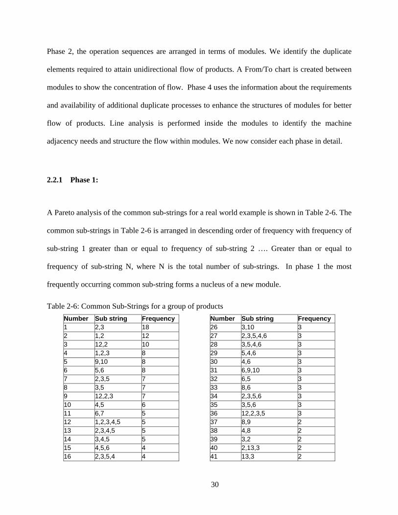
A Pareto analysis of the common sub-strings for a real world example is shown in Table 2-6. The
common sub-strings in Table 2-6 is arranged in descending order of frequency with frequency of
sub-string 1 greater than or equal to frequency of sub-string 2 …. Greater than or equal to
frequency of sub-string N, where N is the total number of sub-strings. In phase 1 the most
frequently occurring common sub-string forms a nucleus of a new module.
Table 2-6: Common Sub-Strings for a group of products Number Sub string Frequency Number Sub string Frequency 1 2,3 18 26 3,10 3 2 1,2 12 27 2,3,5,4,6 3 3 12,2 10 28 3,5,4,6 3 4 1,2,3 8 29 5,4,6 3 5 9,10 8 30 4,6 3 6 5,6 8 31 6,9,10 3 7 2,3,5 7 32 6,5 3 8 3,5 7 33 8,6 3 9 12,2,3 7 34 2,3,5,6 3 10 4,5 6 35 3,5,6 3 11 6,7 5 36 12,2,3,5 3 12 1,2,3,4,5 5 37 8,9 2 13 2,3,4,5 5 38 4,8 2 14 3,4,5 5 39 3,2 2 15 4,5,6 4 40 2,13,3 2 16 2,3,5,4 4 41 13,3 2
30
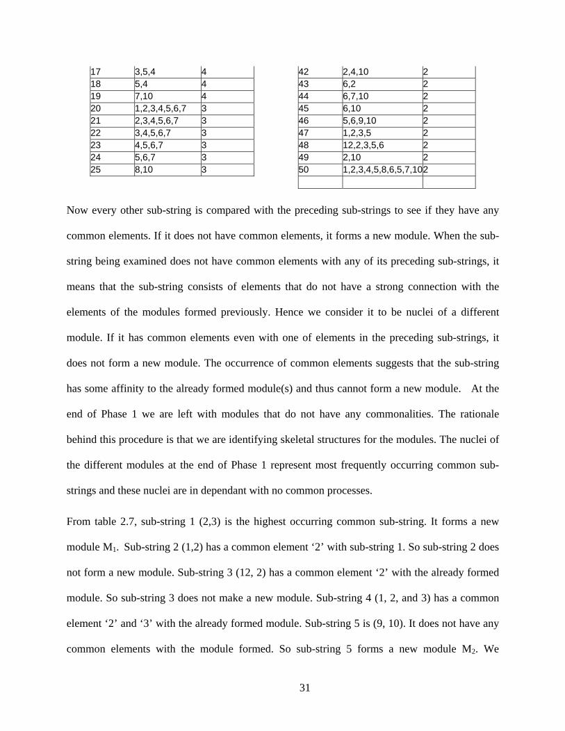
17 3,5,4 4 42 2,4,10 2 18 5,4 4 43 6,2 2 19 7,10 4 44 6,7,10 2 20 1,2,3,4,5,6,7 3 45 6,10 2 21 2,3,4,5,6,7 3 46 5,6,9,10 2 22 3,4,5,6,7 3 47 1,2,3,5 2 23 4,5,6,7 3 48 12,2,3,5,6 2 24 5,6,7 3 49 2,10 2 25 8,10 3 50 1,2,3,4,5,8,6,5,7,102
Now every other sub-string is compared with the preceding sub-strings to see if they have any
common elements. If it does not have common elements, it forms a new module. When the sub-
string being examined does not have common elements with any of its preceding sub-strings, it
means that the sub-string consists of elements that do not have a strong connection with the
elements of the modules formed previously. Hence we consider it to be nuclei of a different
module. If it has common elements even with one of elements in the preceding sub-strings, it
does not form a new module. The occurrence of common elements suggests that the sub-string
has some affinity to the already formed module(s) and thus cannot form a new module. At the
end of Phase 1 we are left with modules that do not have any commonalities. The rationale
behind this procedure is that we are identifying skeletal structures for the modules. The nuclei of
the different modules at the end of Phase 1 represent most frequently occurring common sub-
strings and these nuclei are in dependant with no common processes.
From table 2.7, sub-string 1 (2,3) is the highest occurring common sub-string. It forms a new
module M1. Sub-string 2 (1,2) has a common element ‘2’ with sub-string 1. So sub-string 2 does
not form a new module. Sub-string 3 (12, 2) has a common element ‘2’ with the already formed
module. So sub-string 3 does not make a new module. Sub-string 4 (1, 2, and 3) has a common
element ‘2’ and ‘3’ with the already formed module. Sub-string 5 is (9, 10). It does not have any
common elements with the module formed. So sub-string 5 forms a new module M2. We
31
similarly proceed with rest of the sub-strings. That is we compare each sub-string with the
module formed to find if it has any common elements. If it has no common elements, it forms a
new module. If it has common elements, it does not form a new module. At the end of the
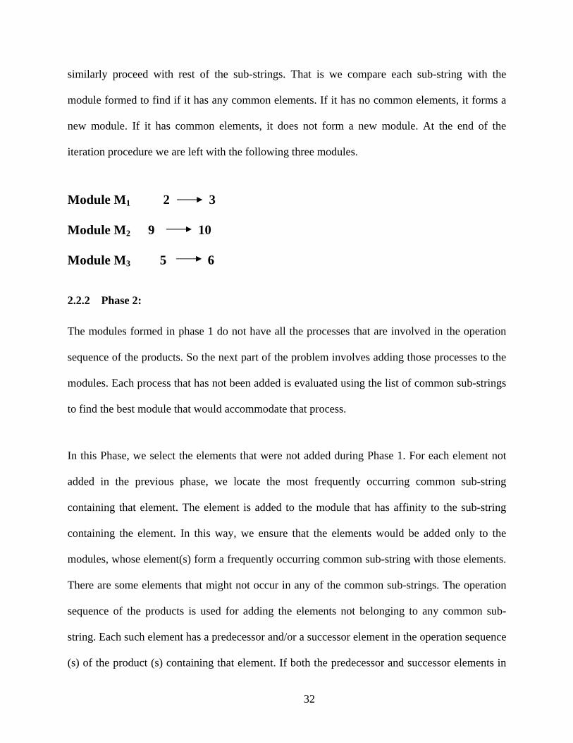
iteration procedure we are left with the following three modules.
Module M1 2 3 Module M2 9 10
Module M3 5 6
2.2.2 Phase 2: The modules formed in phase 1 do not have all the processes that are involved in the operation
sequence of the products. So the next part of the problem involves adding those processes to the
modules. Each process that has not been added is evaluated using the list of common sub-strings
to find the best module that would accommodate that process.
In this Phase, we select the elements that were not added during Phase 1. For each element not
added in the previous phase, we locate the most frequently occurring common sub-string
containing that element. The element is added to the module that has affinity to the sub-string
containing the element. In this way, we ensure that the elements would be added only to the
modules, whose element(s) form a frequently occurring common sub-string with those elements.
There are some elements that might not occur in any of the common sub-strings. The operation
sequence of the products is used for adding the elements not belonging to any common sub-
string. Each such element has a predecessor and/or a successor element in the operation sequence
(s) of the product (s) containing that element. If both the predecessor and successor elements in
32
any of the operation sequence belong to a particular module, the element is added to that module.
This is done to avoid backtracking of the product defined by that operation sequence. If there is
no such operation sequence, the frequency with which the element occurs with the elements of
the different modules is utilized to locate the module that would accommodate the process type
in a better fashion. This ensures that the element has more affinity to the module to which it has
been added.
Elements 1, 4, 7,11,12,13 and 14 were not added to the modules formed at the end of phase 1.
Let us see how phase 2 helps to add the processes to one of the modules formed in phase 1.
Element 1:
First we identify the highest frequency common sub-string that contains element 1. In our case
study it is sub-string 2 (1,2). The sub-string identified is compared with the modules formed in
phase 1 i.e. we identify the module that has elements common with the identified sub-string.
Module 1 has elements 2 and 3. Hence element 1 is added to module 1. Similarly elements 4, 7,
11, 12 and 13 are added to the respective modules following the same procedure.
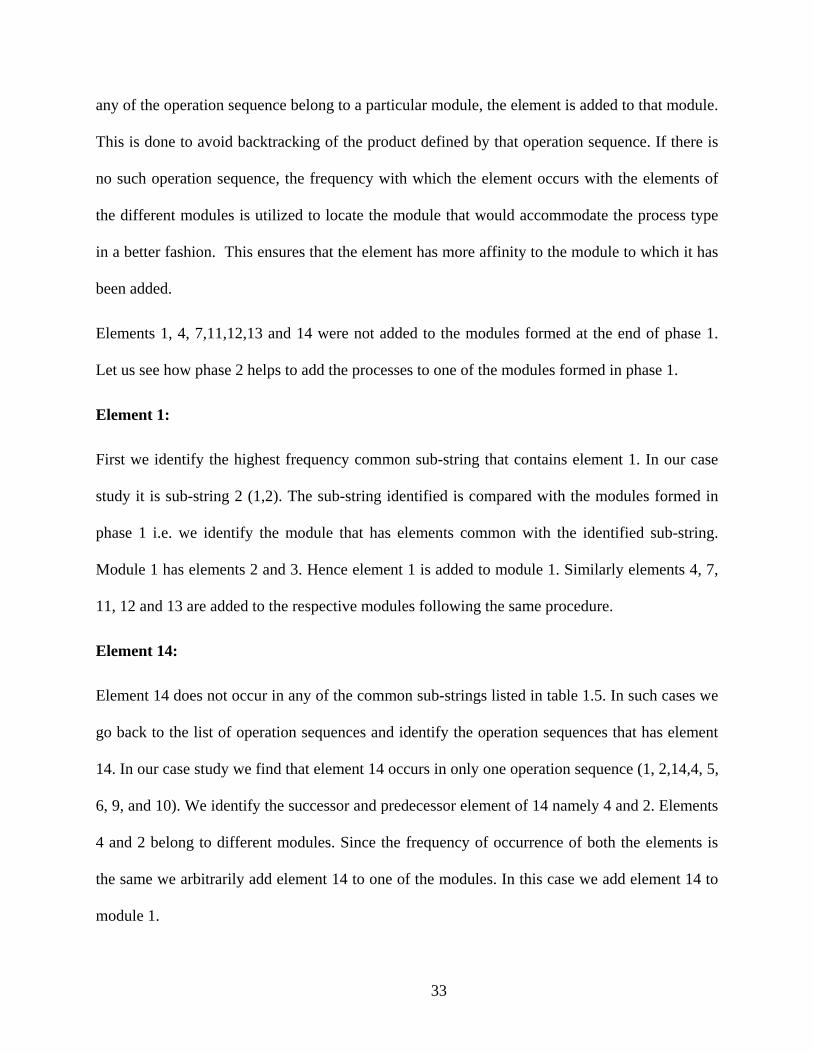
Element 14:
Element 14 does not occur in any of the common sub-strings listed in table 1.5. In such cases we
go back to the list of operation sequences and identify the operation sequences that has element
14. In our case study we find that element 14 occurs in only one operation sequence (1, 2,14,4, 5,
6, 9, and 10). We identify the successor and predecessor element of 14 namely 4 and 2. Elements
4 and 2 belong to different modules. Since the frequency of occurrence of both the elements is
the same we arbitrarily add element 14 to one of the modules. In this case we add element 14 to
module 1.
33
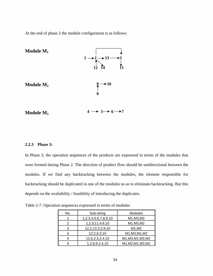
At the end of phase 2 the module configuration is as follows:
1 2 13 3 12 14 11
Module M1
9 10 8
Module M2
4 5 6 7
Module M3
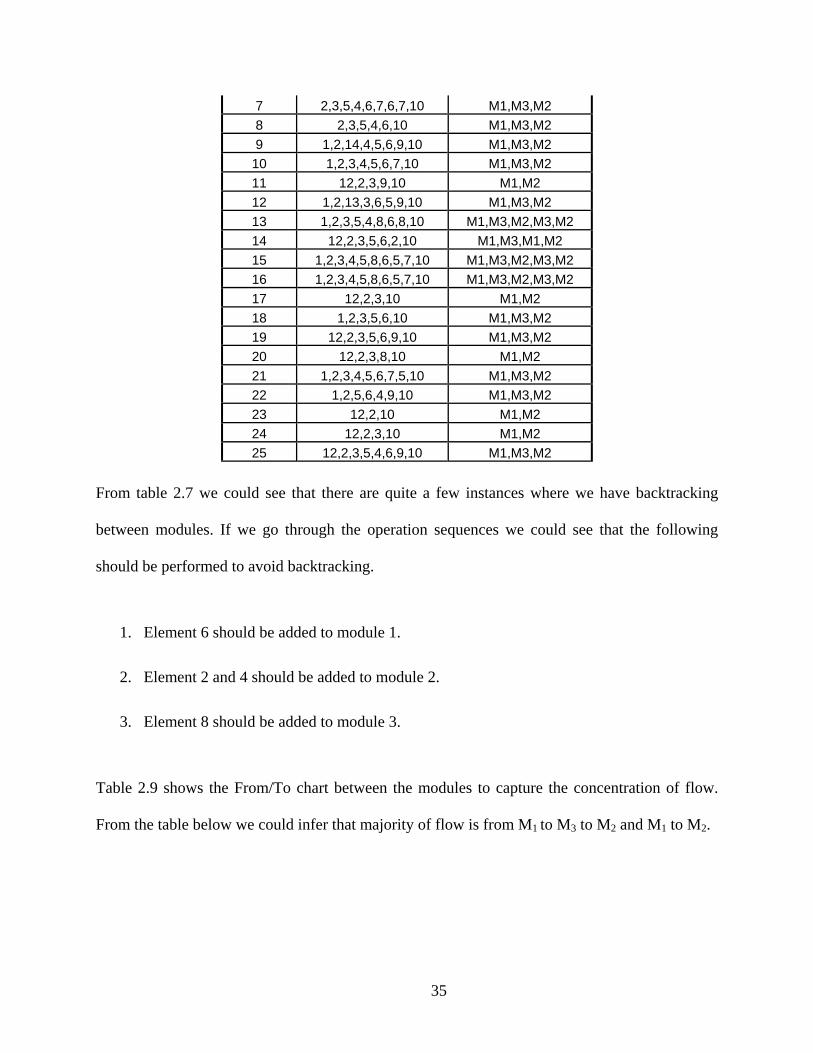
2.2.3 Phase 3: In Phase 3, the operation sequences of the products are expressed in terms of the modules that
were formed during Phase 2. The direction of product flow should be unidirectional between the
modules. If we find any backtracking between the modules, the element responsible for
backtracking should be duplicated in one of the modules so as to eliminate backtracking. But this
depends on the availability / feasibility of introducing the duplicates.
Table 2-7: Operation sequences expressed in terms of modules
No. Sub-string Modules 1 1,2,3,4,5,6,7,8,9,10 M1,M3,M2 2 1,2,3,11,4,8,10 M1,M3,M2 3 12,2,13,3,2,9,10 M1,M2 4 12,2,6,3,10 M1,M3,M1,M2 5 12,6,2,3,2,4,10 M1,M3,M1,M3,M2 6 1,2,8,9,2,4,10 M1,M2,M1,M3,M2
34
7 2,3,5,4,6,7,6,7,10 M1,M3,M2 8 2,3,5,4,6,10 M1,M3,M2 9 1,2,14,4,5,6,9,10 M1,M3,M2
10 1,2,3,4,5,6,7,10 M1,M3,M2 11 12,2,3,9,10 M1,M2 12 1,2,13,3,6,5,9,10 M1,M3,M2 13 1,2,3,5,4,8,6,8,10 M1,M3,M2,M3,M2 14 12,2,3,5,6,2,10 M1,M3,M1,M2 15 1,2,3,4,5,8,6,5,7,10 M1,M3,M2,M3,M2 16 1,2,3,4,5,8,6,5,7,10 M1,M3,M2,M3,M2 17 12,2,3,10 M1,M2 18 1,2,3,5,6,10 M1,M3,M2 19 12,2,3,5,6,9,10 M1,M3,M2 20 12,2,3,8,10 M1,M2 21 1,2,3,4,5,6,7,5,10 M1,M3,M2 22 1,2,5,6,4,9,10 M1,M3,M2 23 12,2,10 M1,M2 24 12,2,3,10 M1,M2 25 12,2,3,5,4,6,9,10 M1,M3,M2
From table 2.7 we could see that there are quite a few instances where we have backtracking
between modules. If we go through the operation sequences we could see that the following
should be performed to avoid backtracking.
1. Element 6 should be added to module 1.
2. Element 2 and 4 should be added to module 2.
3. Element 8 should be added to module 3.
Table 2.9 shows the From/To chart between the modules to capture the concentration of flow.
From the table below we could infer that majority of flow is from M1 to M3 to M2 and M1 to M2.
35
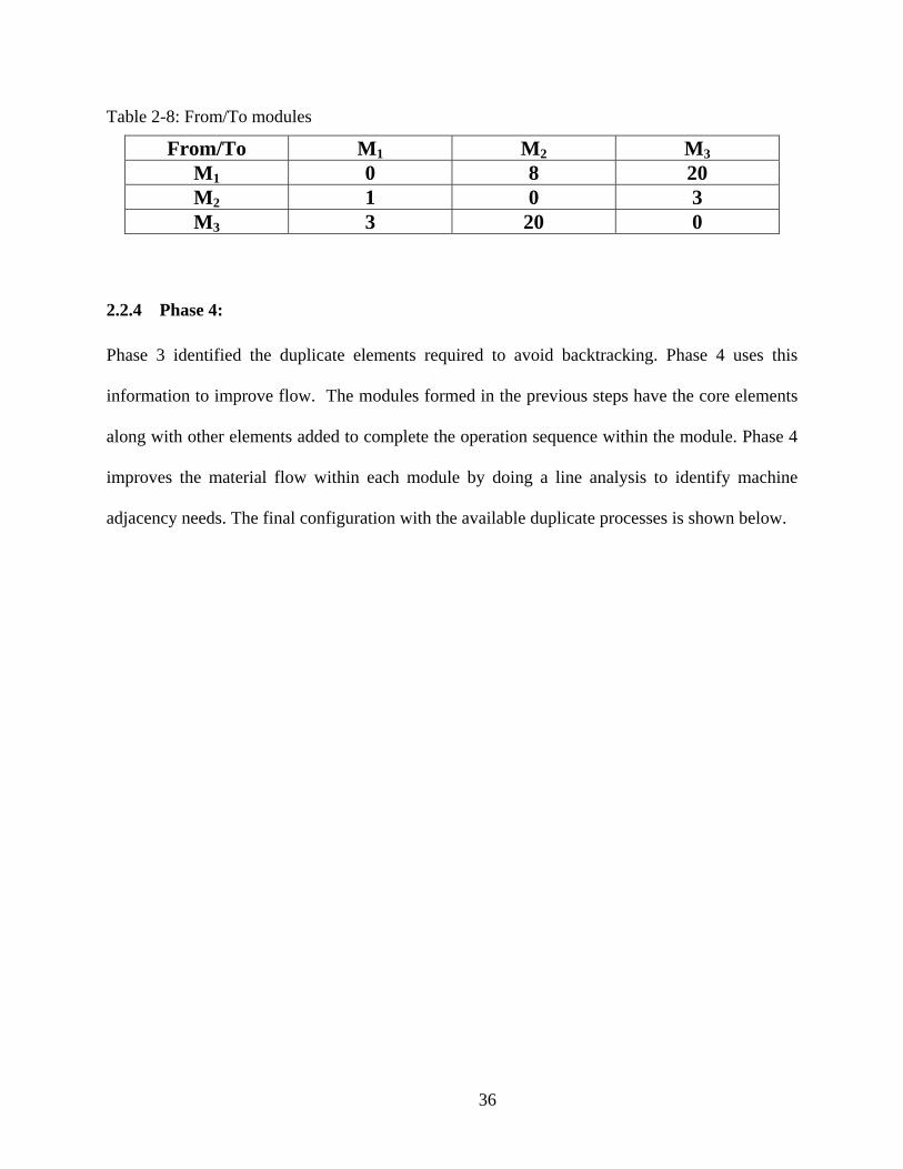
Table 2-8: From/To modules
From/To M1 M2 M3M1 0 8 20 M2 1 0 3 M3 3 20 0
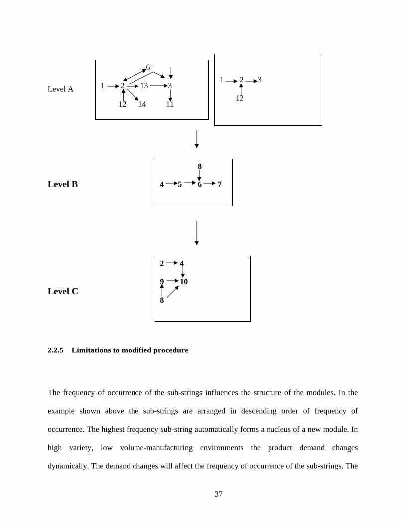
2.2.4 Phase 4: Phase 3 identified the duplicate elements required to avoid backtracking. Phase 4 uses this
information to improve flow. The modules formed in the previous steps have the core elements
along with other elements added to complete the operation sequence within the module. Phase 4
improves the material flow within each module by doing a line analysis to identify machine
adjacency needs. The final configuration with the available duplicate processes is shown below.
36
1 2 3 12
6 1 2 13 3 12 14 11
Level A 8
4 5 6 7
Level B 2 4
9 10 8
Level C
2.2.5 Limitations to modified procedure
The frequency of occurrence of the sub-strings influences the structure of the modules. In the
example shown above the sub-strings are arranged in descending order of frequency of
occurrence. The highest frequency sub-string automatically forms a nucleus of a new module. In
high variety, low volume-manufacturing environments the product demand changes
dynamically. The demand changes will affect the frequency of occurrence of the sub-strings. The
37
changes in frequency will affect the modules formed. Hence the layout configurations have to be
changed as frequently as the frequency of occurrence of sub-string changes. In the example
above (2, 3) is the highest frequency common sub-string. The next highest frequency common
sub-string is (1, 2). Due to demand changes if some products become obsolete then the frequency
of occurrence of the sub-strings changes. If the (1, 2) sub-string becomes the highest frequency
sub-string then the nucleus of the module changes. In order to avoid this problem we have to
consider only those products that have a definite demand over the planning horizon for
engineering analysis. This will make sure that the products will be representative of modules
formed.
The modules formed based on the frequency of the occurrence of the sub-strings determine the
concentration of flow within the facility. For example, module 1 is formed with (8, 7) which is
the highest occurring common sub-string. The frequency of occurrence is 150. The second
module M2 is formed with (3, 4). The frequency of occurrence of this module is 42. You can see
from this example that more products flow through module 1 compared to module 2. This would
tend to create a queuing tendency in front of module 1 making scheduling decisions more
complicated. However in Irani’s procedure one could find that most of the processes are
duplicated in the entire module thereby making flow smooth.
The modules formed using the above procedure does not promote single piece continuous flow.
Batching is almost always unavoidable between modules. This is in contrary to lean
manufacturing which advocate single piece flow.
38
2.3 Comparison between Irani’s procedure and modified procedure
• According to Irani’s procedure [11] if a common sub-string is contained in another
common sub-string the smaller common sub-string will not be considered in the list of
common sub-strings. That is of 1, 2, 3 is a common sub-string and is included within the
common sub-string 1,2,3,4,5,6,7. Hence 1, 2, 3 is not included in the table.
• The modified procedure has a finer breakdown of common sub-strings and the frequency
of occurrence of the sub-strings is used in forming the layout modules.
• In Irani’s procedure, some elements do not form part of any module. These elements are
referred to as residual elements. These elements are located outside the module and parts
that need processing with the element are routed to the element.
• The modified procedure locates the residual elements within the module by looking at the
operation sequence of the part in which the element occurs and identifying the module
that would best enhances the flow with the residual element.
• Table 2-9 shows a comparison on the number of duplicates used by the two procedures.
As you can see that the number of duplicate processes generated by the modified
procedure is less than Irani’s procedure.
39
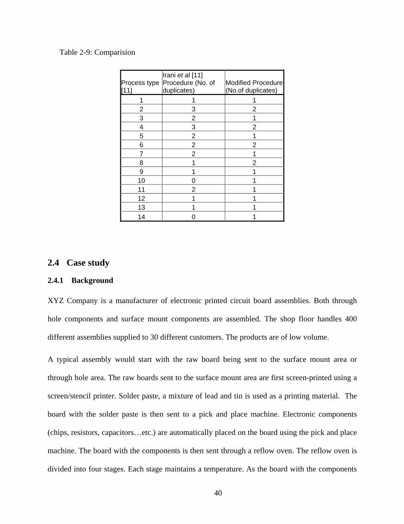
Table 2-9: Comparision
Process type [11]
Irani et al [11] Procedure (No. of duplicates)
Modified Procedure(No.of duplicates)
1 1 1 2 3 2 3 2 1 4 3 2 5 2 1 6 2 2 7 2 1 8 1 2 9 1 1
10 0 1 11 2 1 12 1 1 13 1 1 14 0 1
2.4 Case study
2.4.1 Background XYZ Company is a manufacturer of electronic printed circuit board assemblies. Both through
hole components and surface mount components are assembled. The shop floor handles 400
different assemblies supplied to 30 different customers. The products are of low volume.
A typical assembly would start with the raw board being sent to the surface mount area or
through hole area. The raw boards sent to the surface mount area are first screen-printed using a
screen/stencil printer. Solder paste, a mixture of lead and tin is used as a printing material. The
board with the solder paste is then sent to a pick and place machine. Electronic components
(chips, resistors, capacitors…etc.) are automatically placed on the board using the pick and place
machine. The board with the components is then sent through a reflow oven. The reflow oven is
divided into four stages. Each stage maintains a temperature. As the board with the components
40
and solder paste passes through different stages of the oven, the solder paste melts. Upon cooling
the solder paste melts and fuses with the electronic components making electrical contact. The
boards with the components are then sent to the pre-build/build area where components that
cannot be automatically placed by the machine are hand placed. The boards with the components
are then sent through a wave-soldering machine (a machine that has molten solder flux running
continuously. The boards are sent over the liquid solder wave) to establish electrical contact with
through-hole components.
Subsequently the boards coming out of the wave solder machine are sent for post wave
inspection. This is done to make sure that the boards coming out of the wave solder do not have
any burrs. After wave solder operation the boards are clipped to remove excess solder. From
economy stand point some boards are manufactured in panels. The panels have to be broken
down to get single boards. These operations are carried out at different stages called clipping and
breakout. After clipping and breakout the boards are sent to hardware assembly. The hardware
components are assembled to the boards. After the assembly the boards are sent for in-circuit test
and functional test. Some boards might not have in-circuit test but all boards have functional test.
After the functional test is over the boards are sent for final inspection. The boards are 100%
inspected and if the boards require any rework they are done by the inspectors. All the boards
need not necessarily follow the same path. Some boards might go from post wave to hardware
without clipping and breakout. Some boards might have back tracking i.e. it might have to go to
in circuit test after clipping and come back to break out thereby disrupting the smooth
unidirectional flow.
41
2.4.2 Analysis A preliminary study on the flow of the products revealed the following:
• There is only one wave-soldering machine through which 99% of the boards pass
through. The wave-soldering machine has tremendous capacity. It serves as a
“monument” within the facility. But the high capacity tends to minimize the queue
behind the process. The settings of the wave solder machine have to be changed for each
product. Hence the products have to be batched before they are sent into the wave solder.
• Time study showed that it was not possible to run the product as single piece flow after
the wave-soldering machine. Rather batching it into stages of production proved to be
more effective.
• Study showed that 99% of the products move forward through the plant from the entry as
raw materials to loading dock.
The routings of the assemblies were analyzed using the Rank Order Clustering algorithm. The
final matrix obtained after the iterations did not show the existence of well-defined part/machine
clusters. It was determined that the majority of the boards had two levels of operations: pre-wave
solder operations and post-wave solder operations.
The modified procedure for forming layout modules was applied for the post-wave operations.
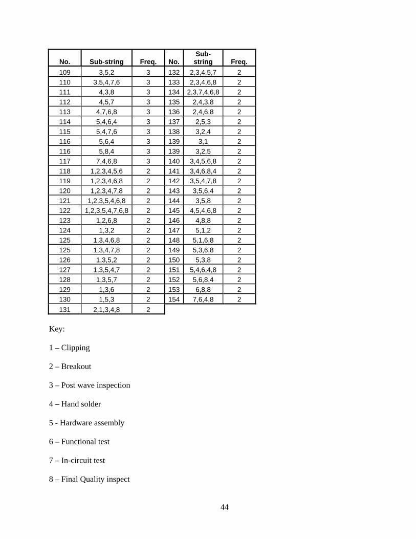
Phase 1: A Pareto analysis of the common sub-strings for XYZ Inc; is shown in table 2.10.
42
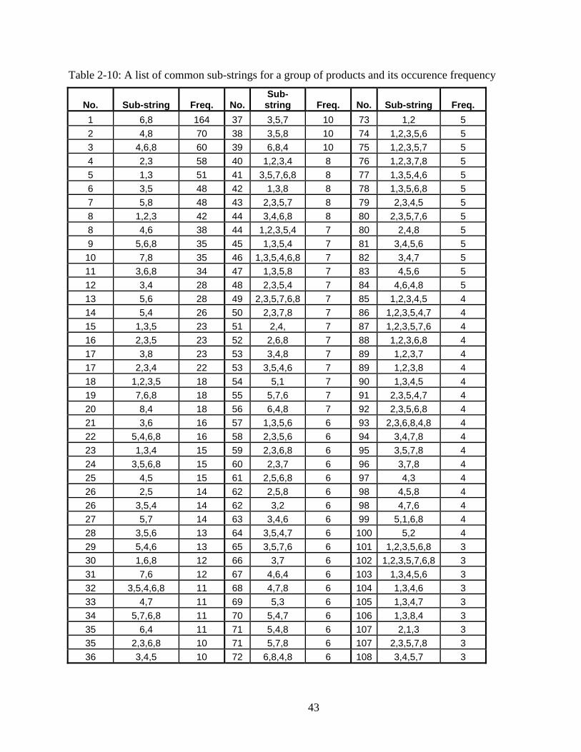
Table 2-10: A list of common sub-strings for a group of products and its occurence frequency
No. Sub-string Freq. No.Sub-
string Freq. No. Sub-string Freq. 1 6,8 164 37 3,5,7 10 73 1,2 5 2 4,8 70 38 3,5,8 10 74 1,2,3,5,6 5 3 4,6,8 60 39 6,8,4 10 75 1,2,3,5,7 5 4 2,3 58 40 1,2,3,4 8 76 1,2,3,7,8 5 5 1,3 51 41 3,5,7,6,8 8 77 1,3,5,4,6 5 6 3,5 48 42 1,3,8 8 78 1,3,5,6,8 5 7 5,8 48 43 2,3,5,7 8 79 2,3,4,5 5 8 1,2,3 42 44 3,4,6,8 8 80 2,3,5,7,6 5 8 4,6 38 44 1,2,3,5,4 7 80 2,4,8 5 9 5,6,8 35 45 1,3,5,4 7 81 3,4,5,6 5 10 7,8 35 46 1,3,5,4,6,8 7 82 3,4,7 5 11 3,6,8 34 47 1,3,5,8 7 83 4,5,6 5 12 3,4 28 48 2,3,5,4 7 84 4,6,4,8 5 13 5,6 28 49 2,3,5,7,6,8 7 85 1,2,3,4,5 4 14 5,4 26 50 2,3,7,8 7 86 1,2,3,5,4,7 4 15 1,3,5 23 51 2,4, 7 87 1,2,3,5,7,6 4 16 2,3,5 23 52 2,6,8 7 88 1,2,3,6,8 4 17 3,8 23 53 3,4,8 7 89 1,2,3,7 4 17 2,3,4 22 53 3,5,4,6 7 89 1,2,3,8 4 18 1,2,3,5 18 54 5,1 7 90 1,3,4,5 4 19 7,6,8 18 55 5,7,6 7 91 2,3,5,4,7 4 20 8,4 18 56 6,4,8 7 92 2,3,5,6,8 4 21 3,6 16 57 1,3,5,6 6 93 2,3,6,8,4,8 4 22 5,4,6,8 16 58 2,3,5,6 6 94 3,4,7,8 4 23 1,3,4 15 59 2,3,6,8 6 95 3,5,7,8 4 24 3,5,6,8 15 60 2,3,7 6 96 3,7,8 4 25 4,5 15 61 2,5,6,8 6 97 4,3 4 26 2,5 14 62 2,5,8 6 98 4,5,8 4 26 3,5,4 14 62 3,2 6 98 4,7,6 4 27 5,7 14 63 3,4,6 6 99 5,1,6,8 4 28 3,5,6 13 64 3,5,4,7 6 100 5,2 4 29 5,4,6 13 65 3,5,7,6 6 101 1,2,3,5,6,8 3 30 1,6,8 12 66 3,7 6 102 1,2,3,5,7,6,8 3 31 7,6 12 67 4,6,4 6 103 1,3,4,5,6 3 32 3,5,4,6,8 11 68 4,7,8 6 104 1,3,4,6 3 33 4,7 11 69 5,3 6 105 1,3,4,7 3 34 5,7,6,8 11 70 5,4,7 6 106 1,3,8,4 3 35 6,4 11 71 5,4,8 6 107 2,1,3 3 35 2,3,6,8 10 71 5,7,8 6 107 2,3,5,7,8 3 36 3,4,5 10 72 6,8,4,8 6 108 3,4,5,7 3
43
No. Sub-string Freq. No.Sub-
string Freq. 109 3,5,2 3 132 2,3,4,5,7 2 110 3,5,4,7,6 3 133 2,3,4,6,8 2 111 4,3,8 3 134 2,3,7,4,6,8 2 112 4,5,7 3 135 2,4,3,8 2 113 4,7,6,8 3 136 2,4,6,8 2 114 5,4,6,4 3 137 2,5,3 2 115 5,4,7,6 3 138 3,2,4 2 116 5,6,4 3 139 3,1 2 116 5,8,4 3 139 3,2,5 2 117 7,4,6,8 3 140 3,4,5,6,8 2 118 1,2,3,4,5,6 2 141 3,4,6,8,4 2 119 1,2,3,4,6,8 2 142 3,5,4,7,8 2 120 1,2,3,4,7,8 2 143 3,5,6,4 2 121 1,2,3,5,4,6,8 2 144 3,5,8 2 122 1,2,3,5,4,7,6,8 2 145 4,5,4,6,8 2 123 1,2,6,8 2 146 4,8,8 2 124 1,3,2 2 147 5,1,2 2 125 1,3,4,6,8 2 148 5,1,6,8 2 125 1,3,4,7,8 2 149 5,3,6,8 2 126 1,3,5,2 2 150 5,3,8 2 127 1,3,5,4,7 2 151 5,4,6,4,8 2 128 1,3,5,7 2 152 5,6,8,4 2 129 1,3,6 2 153 6,8,8 2 130 1,5,3 2 154 7,6,4,8 2 131 2,1,3,4,8 2
Key: 1 – Clipping
2 – Breakout
3 – Post wave inspection
4 – Hand solder
5 - Hardware assembly
6 – Functional test
7 – In-circuit test
8 – Final Quality inspect
44
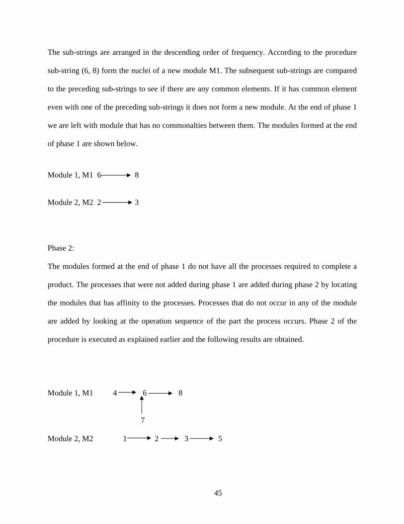
The sub-strings are arranged in the descending order of frequency. According to the procedure
sub-string (6, 8) form the nuclei of a new module M1. The subsequent sub-strings are compared
to the preceding sub-strings to see if there are any common elements. If it has common element
even with one of the preceding sub-strings it does not form a new module. At the end of phase 1
we are left with module that has no commonalties between them. The modules formed at the end
of phase 1 are shown below.
Module 1, M1 6 8 Module 2, M2 2 3 Phase 2: The modules formed at the end of phase 1 do not have all the processes required to complete a
product. The processes that were not added during phase 1 are added during phase 2 by locating
the modules that has affinity to the processes. Processes that do not occur in any of the module
are added by looking at the operation sequence of the part the process occurs. Phase 2 of the
procedure is executed as explained earlier and the following results are obtained.
Module 1, M1 4 6 8 7 Module 2, M2 1 2 3 5
45
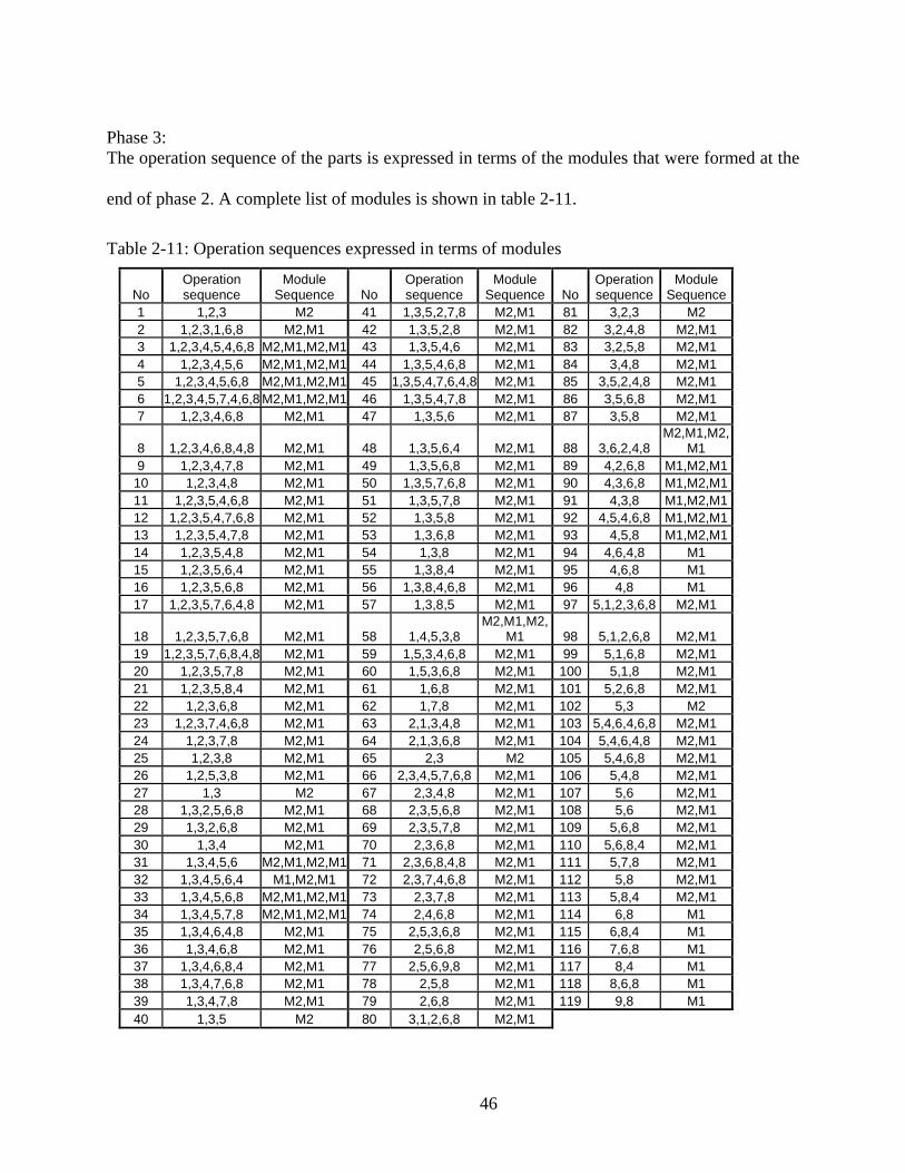
Phase 3: The operation sequence of the parts is expressed in terms of the modules that were formed at the
end of phase 2. A complete list of modules is shown in table 2-11.
Table 2-11: Operation sequences expressed in terms of modules
No Operation sequence
Module Sequence No
Operation sequence
Module Sequence No
Operation sequence
Module Sequence
1 1,2,3 M2 41 1,3,5,2,7,8 M2,M1 81 3,2,3 M2 2 1,2,3,1,6,8 M2,M1 42 1,3,5,2,8 M2,M1 82 3,2,4,8 M2,M1 3 1,2,3,4,5,4,6,8 M2,M1,M2,M1 43 1,3,5,4,6 M2,M1 83 3,2,5,8 M2,M1 4 1,2,3,4,5,6 M2,M1,M2,M1 44 1,3,5,4,6,8 M2,M1 84 3,4,8 M2,M1 5 1,2,3,4,5,6,8 M2,M1,M2,M1 45 1,3,5,4,7,6,4,8 M2,M1 85 3,5,2,4,8 M2,M1 6 1,2,3,4,5,7,4,6,8 M2,M1,M2,M1 46 1,3,5,4,7,8 M2,M1 86 3,5,6,8 M2,M1 7 1,2,3,4,6,8 M2,M1 47 1,3,5,6 M2,M1 87 3,5,8 M2,M1
8 1,2,3,4,6,8,4,8 M2,M1 48 1,3,5,6,4 M2,M1 88 3,6,2,4,8 M2,M1,M2,
M1 9 1,2,3,4,7,8 M2,M1 49 1,3,5,6,8 M2,M1 89 4,2,6,8 M1,M2,M1
10 1,2,3,4,8 M2,M1 50 1,3,5,7,6,8 M2,M1 90 4,3,6,8 M1,M2,M1 11 1,2,3,5,4,6,8 M2,M1 51 1,3,5,7,8 M2,M1 91 4,3,8 M1,M2,M1 12 1,2,3,5,4,7,6,8 M2,M1 52 1,3,5,8 M2,M1 92 4,5,4,6,8 M1,M2,M1 13 1,2,3,5,4,7,8 M2,M1 53 1,3,6,8 M2,M1 93 4,5,8 M1,M2,M1 14 1,2,3,5,4,8 M2,M1 54 1,3,8 M2,M1 94 4,6,4,8 M1 15 1,2,3,5,6,4 M2,M1 55 1,3,8,4 M2,M1 95 4,6,8 M1 16 1,2,3,5,6,8 M2,M1 56 1,3,8,4,6,8 M2,M1 96 4,8 M1 17 1,2,3,5,7,6,4,8 M2,M1 57 1,3,8,5 M2,M1 97 5,1,2,3,6,8 M2,M1
18 1,2,3,5,7,6,8 M2,M1 58 1,4,5,3,8 M2,M1,M2,
M1 98 5,1,2,6,8 M2,M1 19 1,2,3,5,7,6,8,4,8 M2,M1 59 1,5,3,4,6,8 M2,M1 99 5,1,6,8 M2,M1 20 1,2,3,5,7,8 M2,M1 60 1,5,3,6,8 M2,M1 100 5,1,8 M2,M1 21 1,2,3,5,8,4 M2,M1 61 1,6,8 M2,M1 101 5,2,6,8 M2,M1 22 1,2,3,6,8 M2,M1 62 1,7,8 M2,M1 102 5,3 M2 23 1,2,3,7,4,6,8 M2,M1 63 2,1,3,4,8 M2,M1 103 5,4,6,4,6,8 M2,M1 24 1,2,3,7,8 M2,M1 64 2,1,3,6,8 M2,M1 104 5,4,6,4,8 M2,M1 25 1,2,3,8 M2,M1 65 2,3 M2 105 5,4,6,8 M2,M1 26 1,2,5,3,8 M2,M1 66 2,3,4,5,7,6,8 M2,M1 106 5,4,8 M2,M1 27 1,3 M2 67 2,3,4,8 M2,M1 107 5,6 M2,M1 28 1,3,2,5,6,8 M2,M1 68 2,3,5,6,8 M2,M1 108 5,6 M2,M1 29 1,3,2,6,8 M2,M1 69 2,3,5,7,8 M2,M1 109 5,6,8 M2,M1 30 1,3,4 M2,M1 70 2,3,6,8 M2,M1 110 5,6,8,4 M2,M1 31 1,3,4,5,6 M2,M1,M2,M1 71 2,3,6,8,4,8 M2,M1 111 5,7,8 M2,M1 32 1,3,4,5,6,4 M1,M2,M1 72 2,3,7,4,6,8 M2,M1 112 5,8 M2,M1 33 1,3,4,5,6,8 M2,M1,M2,M1 73 2,3,7,8 M2,M1 113 5,8,4 M2,M1 34 1,3,4,5,7,8 M2,M1,M2,M1 74 2,4,6,8 M2,M1 114 6,8 M1 35 1,3,4,6,4,8 M2,M1 75 2,5,3,6,8 M2,M1 115 6,8,4 M1 36 1,3,4,6,8 M2,M1 76 2,5,6,8 M2,M1 116 7,6,8 M1 37 1,3,4,6,8,4 M2,M1 77 2,5,6,9,8 M2,M1 117 8,4 M1 38 1,3,4,7,6,8 M2,M1 78 2,5,8 M2,M1 118 8,6,8 M1 39 1,3,4,7,8 M2,M1 79 2,6,8 M2,M1 119 9,8 M1 40 1,3,5 M2 80 3,1,2,6,8 M2,M1
46
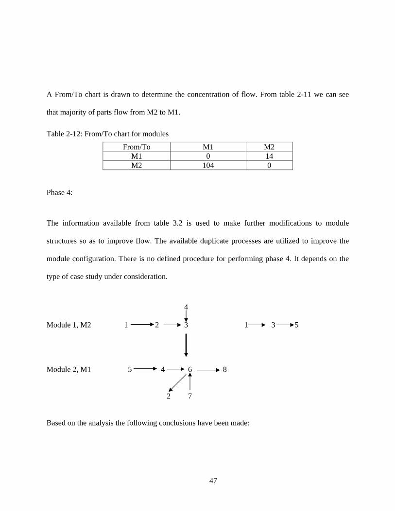
A From/To chart is drawn to determine the concentration of flow. From table 2-11 we can see
that majority of parts flow from M2 to M1.
Table 2-12: From/To chart for modules
From/To M1 M2 M1 0 14 M2 104 0
Phase 4:
The information available from table 3.2 is used to make further modifications to module
structures so as to improve flow. The available duplicate processes are utilized to improve the
module configuration. There is no defined procedure for performing phase 4. It depends on the
type of case study under consideration.
4 Module 1, M2 1 2 3 1 3 5 Module 2, M1 5 4 6 8 2 7 Based on the analysis the following conclusions have been made:
47
1. The flow shop should be split into two parts: one before the wave soldering machine and
one after the wave-soldering machine.
2. It is possible to run the product as single piece flow before the wave-soldering machine.
3. Products have to be batched before going through the wave-soldering machine. First In
System First Out (FISFO) is used to control ties.
4. Products coming out of the wave-soldering machine have to be batched again and sent
through different stages before being shipped.
The following were implemented based on the conclusions:
The job shop has three cells before the wave-soldering machine. Cell 1 has a screen printer, pick
and place machine, reflow oven, a pre-build and a build table. Cell 2 is a duplication of cell 1 to
meet capacity. Cell 3 has a DIP machine, VCD machine for mounting resistors and capacitors, a
LCD machine used for similar purpose, a pre-build and a build table. The cells before the wave-
soldering machine are considered to be stage 1. Any product entering the facility will run
through one of the three cells. Products get batched after they come out of the cell. FISFO is used
to break the ties while sending the products through the wave-soldering machine.
The wave-soldering machine is considered to be stage 2.
The products coming out of the wave-soldering machine is batched and sent to either of the 2
cells in stage 3. Cell 4 consists of clipping, breakout and post-wave inspection. Cell 5 consists of
clipping and post-wave inspection. These machines are duplicated in both the cells to meet
capacity and to maintain single piece flow within each stage.
48

Stage 4 has 3 cells. Cell 6 has a hardware assembly, a functional test machine, and an in-circuit
test machine. Cell 7 has hardware assembly, and in-circuit Cell 8 has hardware assembly, a
functional test, an in-circuit test and a breakout machine.
Copyright © Mohan Swaminathan 2004
49
Chapter 3 Hybrid Flow Shop in the context of lean operations
In a hybrid flow shop layout (HFS), machines are arranged in groups and the groups are
contained within a secondary structure called modules. The modules in a hybrid flow shop layout
are the highest-level structure and they are arranged in a sequence to avoid back tracking. One
module may contain multiple groups. The groups within the modules represent major sub-
sequences of operations.
The machines selected to comprise a group are based on common sub-strings, i.e., portions of the
routings that multiple products share. Ideally the products pass through these machines in the
order of the given substring, but physical layout of the machines may be used to accommodate
multiple substrings while avoiding replication of the machines.
Each group of machines does not process the whole of a product. Instead the products are taken
through stages of manufacturing. Each stage performs one or more consecutive operations of
almost every part routed through it. Generally we prefer the routing of a product to flow between
groups in separate modules. Cross flow might exist between the groups within a module.
Although it is desirable to avoid cross flow, if replication is an issue it may be necessary to have
cross flow between adjacent groups within a given module. If necessary, relocation and
orientation ideas can be applied to simplify cross flow between groups.
In general, the flow of a product would proceed sequentially through the modules, a product
visiting a single group within each module, completing the required processing as it passes
through the modules. Cross-flows of products between groups in a single module is permitted,
50
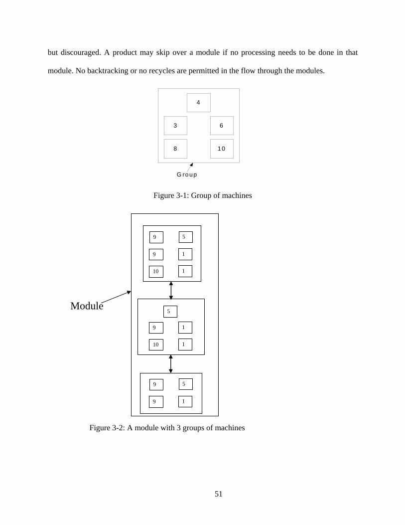
but discouraged. A product may skip over a module if no processing needs to be done in that
module. No backtracking or no recycles are permitted in the flow through the modules.
10
6
4
3
8
G roup
Figure 3-1: Group of machines
Module
9
9
10
5
1
1
9
10
5
1
1
9
9
5
1
Figure 3-2: A module with 3 groups of machines
51
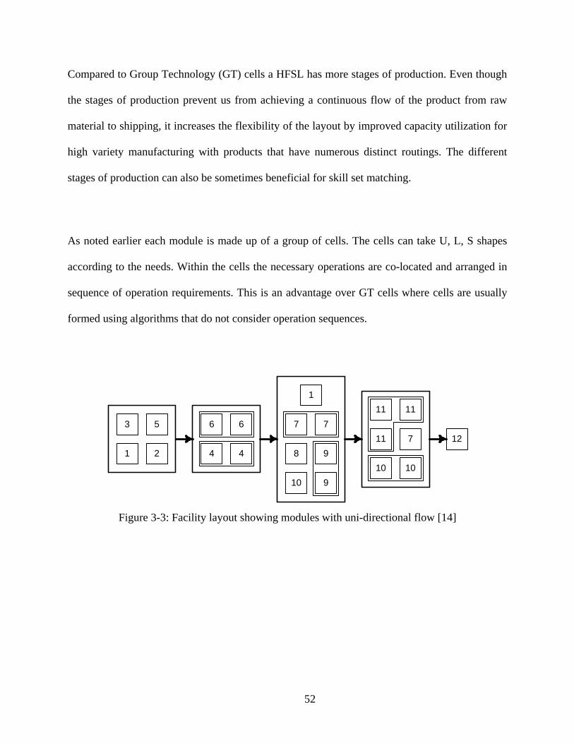
Compared to Group Technology (GT) cells a HFSL has more stages of production. Even though
the stages of production prevent us from achieving a continuous flow of the product from raw
material to shipping, it increases the flexibility of the layout by improved capacity utilization for
high variety manufacturing with products that have numerous distinct routings. The different
stages of production can also be sometimes beneficial for skill set matching.
As noted earlier each module is made up of a group of cells. The cells can take U, L, S shapes
according to the needs. Within the cells the necessary operations are co-located and arranged in
sequence of operation requirements. This is an advantage over GT cells where cells are usually
formed using algorithms that do not consider operation sequences.
1
53127
2 4
66
4
77
98
910
1
1010
11
11
11
Figure 3-3: Facility layout showing modules with uni-directional flow [14]
52
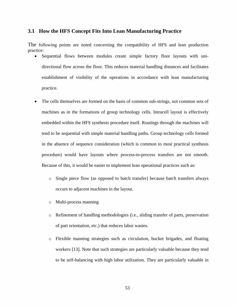
3.1 How the HFS Concept Fits Into Lean Manufacturing Practice The following points are noted concerning the compatibility of HFS and lean production practice:
• Sequential flows between modules create simple factory floor layouts with uni-
directional flow across the floor. This reduces material handling distances and facilitates
establishment of visibility of the operations in accordance with lean manufacturing
practice.
• The cells themselves are formed on the basis of common sub-strings, not common sets of
machines as in the formations of group technology cells. Intracell layout is effectively
embedded within the HFS synthesis procedure itself. Routings through the machines will
tend to be sequential with simple material handling paths. Group technology cells formed
in the absence of sequence consideration (which is common to most practical synthesis
procedure) would have layouts where process-to-process transfers are not smooth.
Because of this, it would be easier to implement lean operational practices such as:
o Single piece flow (as opposed to batch transfer) because batch transfers always
occurs to adjacent machines in the layout.
o Multi-process manning
o Refinement of handling methodologies (i.e., sliding transfer of parts, preservation
of part orientation, etc.) that reduces labor wastes.
o Flexible manning strategies such as circulation, bucket brigades, and floating
workers [13]. Note that such strategies are particularly valuable because they tend
to be self-balancing with high labor utilization. They are particularly valuable in
53
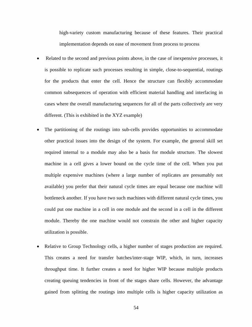
high-variety custom manufacturing because of these features. Their practical
implementation depends on ease of movement from process to process
• Related to the second and previous points above, in the case of inexpensive processes, it
is possible to replicate such processes resulting in simple, close-to-sequential, routings
for the products that enter the cell. Hence the structure can flexibly accommodate
common subsequences of operation with efficient material handling and interfacing in
cases where the overall manufacturing sequences for all of the parts collectively are very
different. (This is exhibited in the XYZ example)
• The partitioning of the routings into sub-cells provides opportunities to accommodate
other practical issues into the design of the system. For example, the general skill set
required internal to a module may also be a basis for module structure. The slowest
machine in a cell gives a lower bound on the cycle time of the cell. When you put
multiple expensive machines (where a large number of replicates are presumably not
available) you prefer that their natural cycle times are equal because one machine will
bottleneck another. If you have two such machines with different natural cycle times, you
could put one machine in a cell in one module and the second in a cell in the different
module. Thereby the one machine would not constrain the other and higher capacity
utilization is possible.
• Relative to Group Technology cells, a higher number of stages production are required.
This creates a need for transfer batches/inter-stage WIP, which, in turn, increases
throughput time. It further creates a need for higher WIP because multiple products
creating queuing tendencies in front of the stages share cells. However, the advantage
gained from splitting the routings into multiple cells is higher capacity utilization as
54
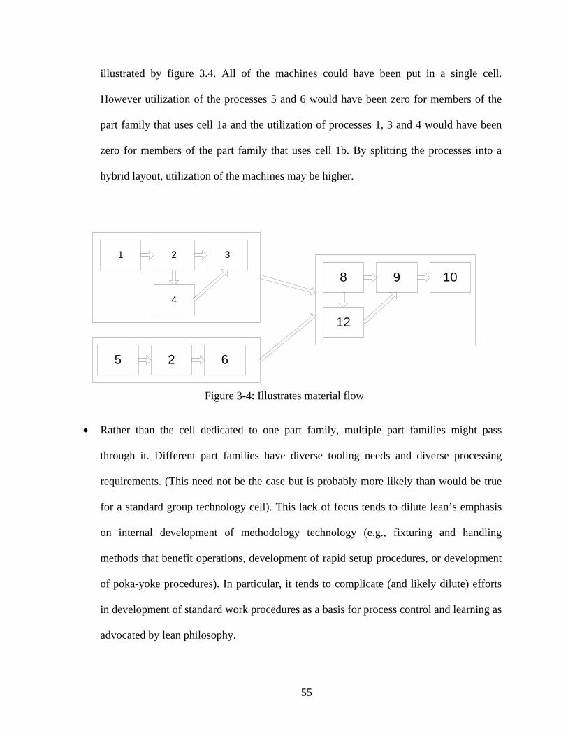
illustrated by figure 3.4. All of the machines could have been put in a single cell.
However utilization of the processes 5 and 6 would have been zero for members of the
part family that uses cell 1a and the utilization of processes 1, 3 and 4 would have been
zero for members of the part family that uses cell 1b. By splitting the processes into a
hybrid layout, utilization of the machines may be higher.
1 2
4
3
5 2 6
8 9
12
10
Figure 3-4: Illustrates material flow
• Rather than the cell dedicated to one part family, multiple part families might pass
through it. Different part families have diverse tooling needs and diverse processing
requirements. (This need not be the case but is probably more likely than would be true
for a standard group technology cell). This lack of focus tends to dilute lean’s emphasis
on internal development of methodology technology (e.g., fixturing and handling
methods that benefit operations, development of rapid setup procedures, or development
of poka-yoke procedures). In particular, it tends to complicate (and likely dilute) efforts
in development of standard work procedures as a basis for process control and learning as
advocated by lean philosophy.
55
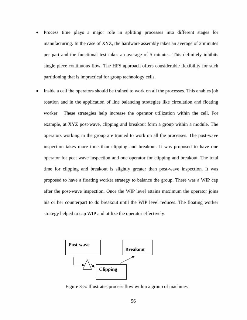
• Process time plays a major role in splitting processes into different stages for
manufacturing. In the case of XYZ, the hardware assembly takes an average of 2 minutes
per part and the functional test takes an average of 5 minutes. This definitely inhibits
single piece continuous flow. The HFS approach offers considerable flexibility for such
partitioning that is impractical for group technology cells.
• Inside a cell the operators should be trained to work on all the processes. This enables job
rotation and in the application of line balancing strategies like circulation and floating
worker. These strategies help increase the operator utilization within the cell. For
example, at XYZ post-wave, clipping and breakout form a group within a module. The
operators working in the group are trained to work on all the processes. The post-wave
inspection takes more time than clipping and breakout. It was proposed to have one
operator for post-wave inspection and one operator for clipping and breakout. The total
time for clipping and breakout is slightly greater than post-wave inspection. It was
proposed to have a floating worker strategy to balance the group. There was a WIP cap
after the post-wave inspection. Once the WIP level attains maximum the operator joins
his or her counterpart to do breakout until the WIP level reduces. The floating worker
strategy helped to cap WIP and utilize the operator effectively.
Breakout Post-wave
Clipping
Figure 3-5: Illustrates process flow within a group of machines
56
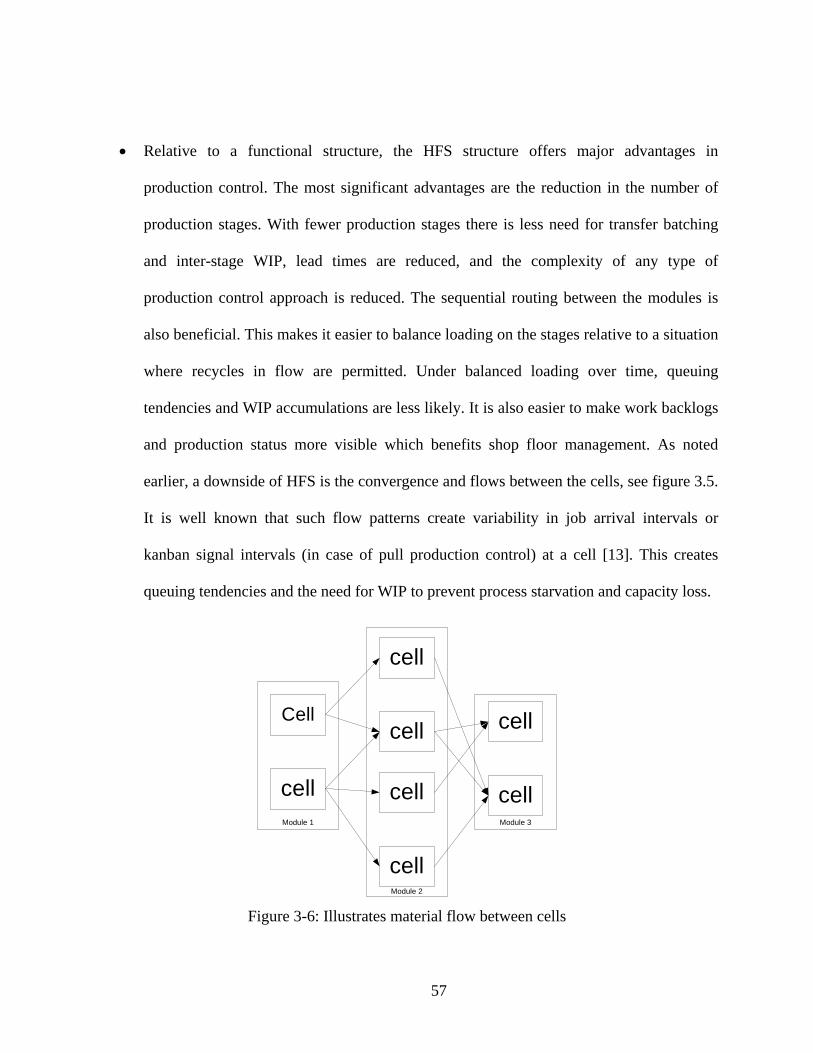
• Relative to a functional structure, the HFS structure offers major advantages in
production control. The most significant advantages are the reduction in the number of
production stages. With fewer production stages there is less need for transfer batching
and inter-stage WIP, lead times are reduced, and the complexity of any type of
production control approach is reduced. The sequential routing between the modules is
also beneficial. This makes it easier to balance loading on the stages relative to a situation
where recycles in flow are permitted. Under balanced loading over time, queuing
tendencies and WIP accumulations are less likely. It is also easier to make work backlogs
and production status more visible which benefits shop floor management. As noted
earlier, a downside of HFS is the convergence and flows between the cells, see figure 3.5.
It is well known that such flow patterns create variability in job arrival intervals or
kanban signal intervals (in case of pull production control) at a cell [13]. This creates
queuing tendencies and the need for WIP to prevent process starvation and capacity loss.
Cell
cell
cell
cell
cell
cell
cell
cellModule 1
Module 2
Module 3
Figure 3-6: Illustrates material flow between cells
57
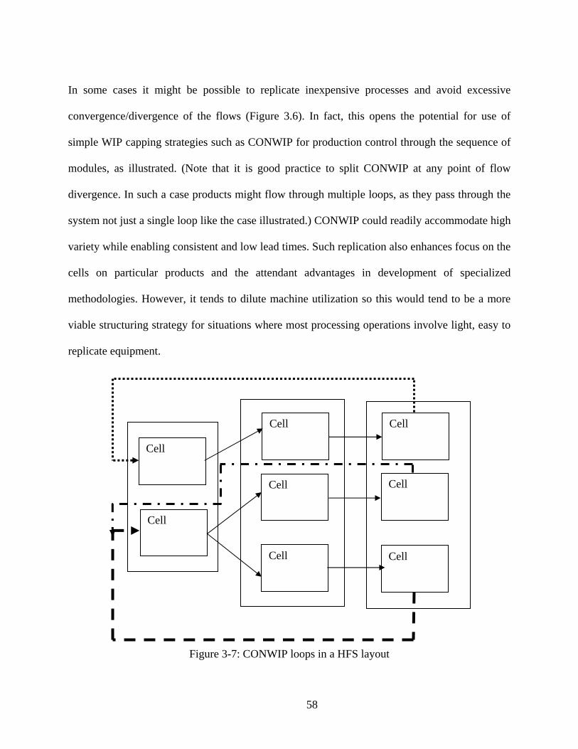
In some cases it might be possible to replicate inexpensive processes and avoid excessive
convergence/divergence of the flows (Figure 3.6). In fact, this opens the potential for use of
simple WIP capping strategies such as CONWIP for production control through the sequence of
modules, as illustrated. (Note that it is good practice to split CONWIP at any point of flow
divergence. In such a case products might flow through multiple loops, as they pass through the
system not just a single loop like the case illustrated.) CONWIP could readily accommodate high
variety while enabling consistent and low lead times. Such replication also enhances focus on the
cells on particular products and the attendant advantages in development of specialized
methodologies. However, it tends to dilute machine utilization so this would tend to be a more
viable structuring strategy for situations where most processing operations involve light, easy to
replicate equipment.
Cell
Cell
Cell Cell
Cell
Cell Cell
Figure 3-7: CONWIP loops in a HFS layout
Cell
58
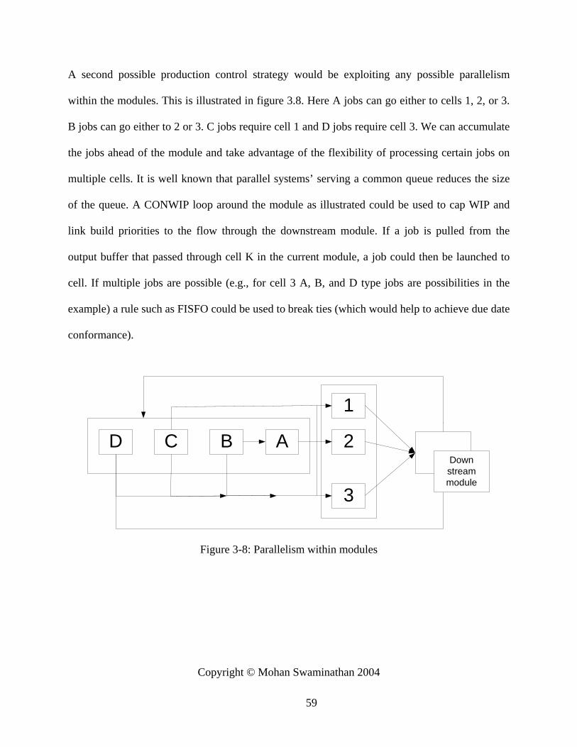
A second possible production control strategy would be exploiting any possible parallelism
within the modules. This is illustrated in figure 3.8. Here A jobs can go either to cells 1, 2, or 3.
B jobs can go either to 2 or 3. C jobs require cell 1 and D jobs require cell 3. We can accumulate
the jobs ahead of the module and take advantage of the flexibility of processing certain jobs on
multiple cells. It is well known that parallel systems’ serving a common queue reduces the size
of the queue. A CONWIP loop around the module as illustrated could be used to cap WIP and
link build priorities to the flow through the downstream module. If a job is pulled from the
output buffer that passed through cell K in the current module, a job could then be launched to
cell. If multiple jobs are possible (e.g., for cell 3 A, B, and D type jobs are possibilities in the
example) a rule such as FISFO could be used to break ties (which would help to achieve due date
conformance).
D C B A
1
2
3
Downstreammodule
Figure 3-8: Parallelism within modules
Copyright © Mohan Swaminathan 2004
59
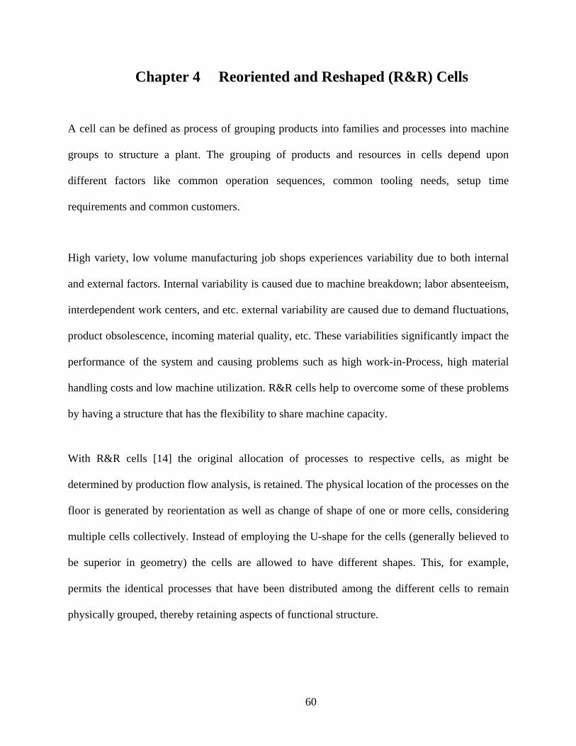
Chapter 4 Reoriented and Reshaped (R&R) Cells
A cell can be defined as process of grouping products into families and processes into machine
groups to structure a plant. The grouping of products and resources in cells depend upon
different factors like common operation sequences, common tooling needs, setup time
requirements and common customers.
High variety, low volume manufacturing job shops experiences variability due to both internal
and external factors. Internal variability is caused due to machine breakdown; labor absenteeism,
interdependent work centers, and etc. external variability are caused due to demand fluctuations,
product obsolescence, incoming material quality, etc. These variabilities significantly impact the
performance of the system and causing problems such as high work-in-Process, high material
handling costs and low machine utilization. R&R cells help to overcome some of these problems
by having a structure that has the flexibility to share machine capacity.
With R&R cells [14] the original allocation of processes to respective cells, as might be
determined by production flow analysis, is retained. The physical location of the processes on the
floor is generated by reorientation as well as change of shape of one or more cells, considering
multiple cells collectively. Instead of employing the U-shape for the cells (generally believed to
be superior in geometry) the cells are allowed to have different shapes. This, for example,
permits the identical processes that have been distributed among the different cells to remain
physically grouped, thereby retaining aspects of functional structure.
60
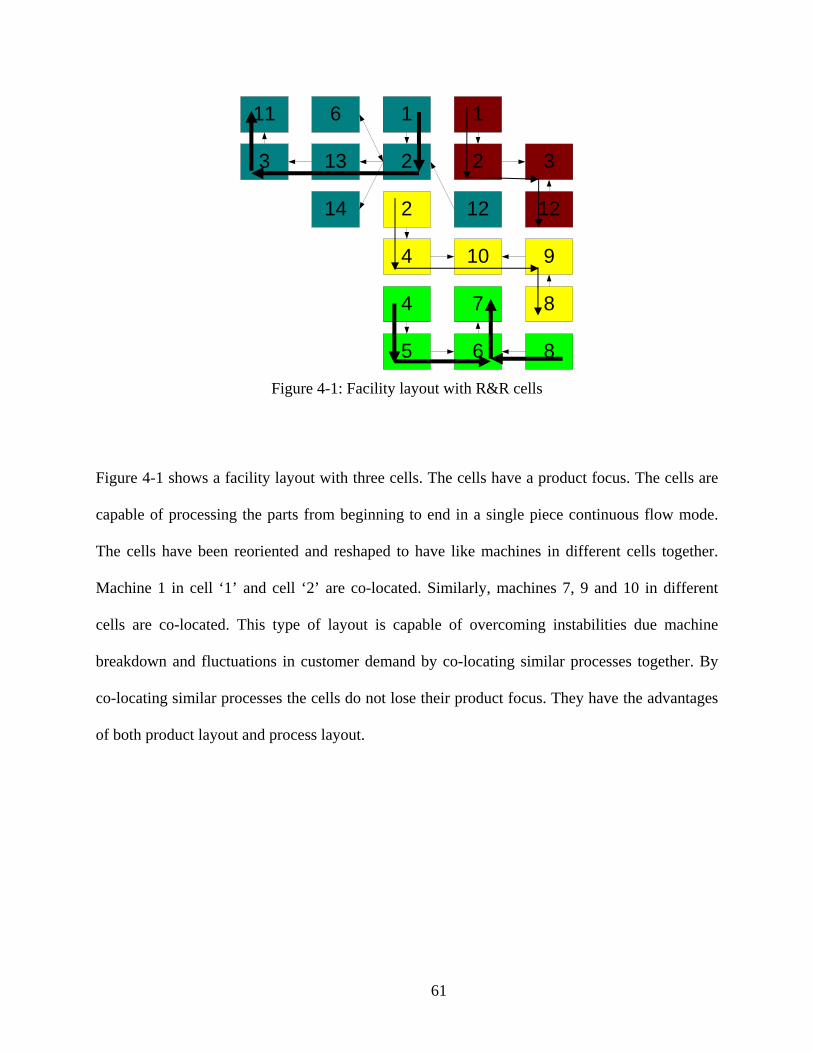
13
14
2
2
2
12
3
12
6
3
4
4
10
7
9
8
11 1
5
1
6 8
Figure 4-1: Facility layout with R&R cells
Figure 4-1 shows a facility layout with three cells. The cells have a product focus. The cells are
capable of processing the parts from beginning to end in a single piece continuous flow mode.
The cells have been reoriented and reshaped to have like machines in different cells together.
Machine 1 in cell ‘1’ and cell ‘2’ are co-located. Similarly, machines 7, 9 and 10 in different
cells are co-located. This type of layout is capable of overcoming instabilities due machine
breakdown and fluctuations in customer demand by co-locating similar processes together. By
co-locating similar processes the cells do not lose their product focus. They have the advantages
of both product layout and process layout.
61

4.1 Example of Forming R&R Cells The modified procedure for forming layout modules can be used to explain the formation of
R&R cells for high variety, low volume manufacturing. At the end of the procedure the
following modules were formed as shown below:
6 1 2 13 3 12 14 11
1 2 3 12
Level A 8
4 5 6 7
Level B
2 4 9 10 8
Level C The modules formed at the end of the phase 4 are so arranged to promote uni-directional flow of
products. Any backtracking in between modules is avoided by duplicating the process. The
62
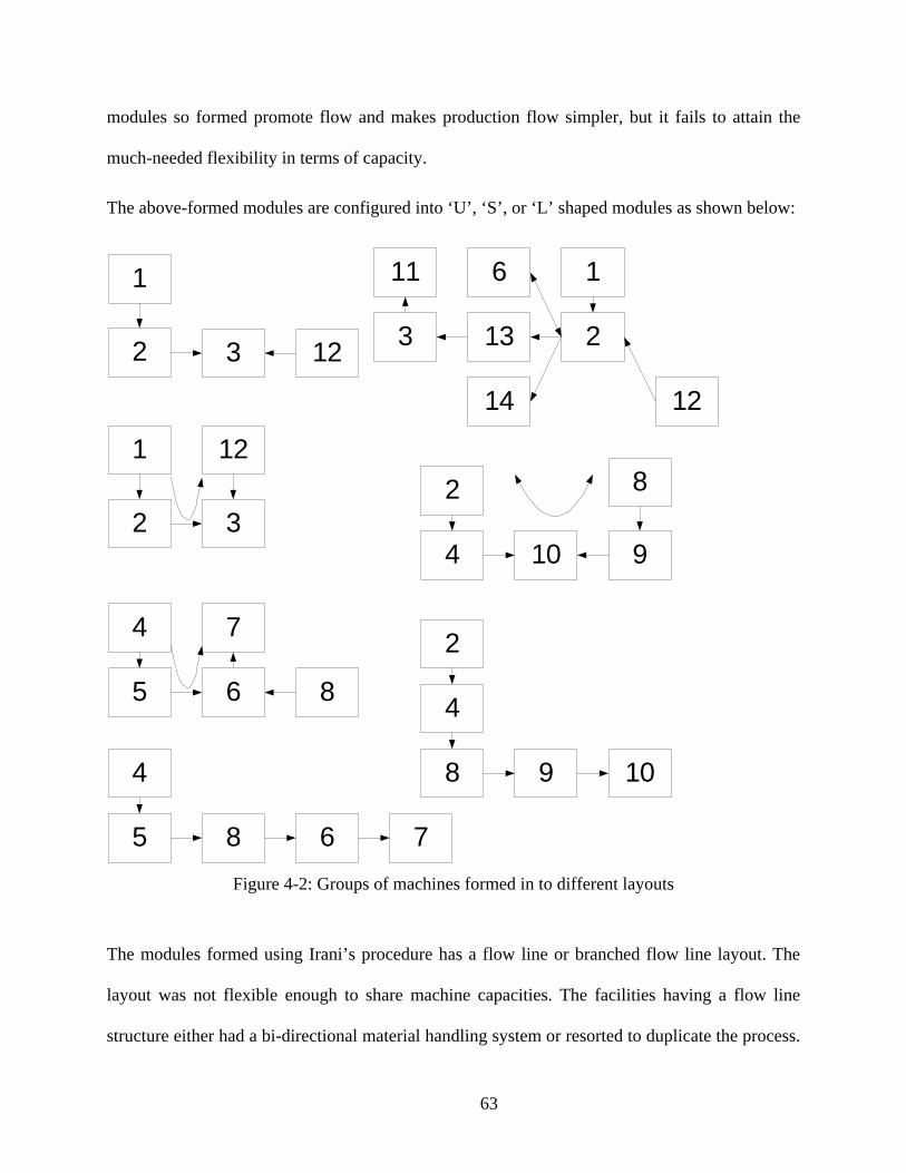
modules so formed promote flow and makes production flow simpler, but it fails to attain the
much-needed flexibility in terms of capacity.
The above-formed modules are configured into ‘U’, ‘S’, or ‘L’ shaped modules as shown below:
13
14
2
22
12
3
12
6
3
4
4
10
7
9
8
11 1
5
1
6 8
2 3 12
1
4
65 8 7
2
4
1098
Figure 4-2: Groups of machines formed in to different layouts
The modules formed using Irani’s procedure has a flow line or branched flow line layout. The
layout was not flexible enough to share machine capacities. The facilities having a flow line
structure either had a bi-directional material handling system or resorted to duplicate the process.
63
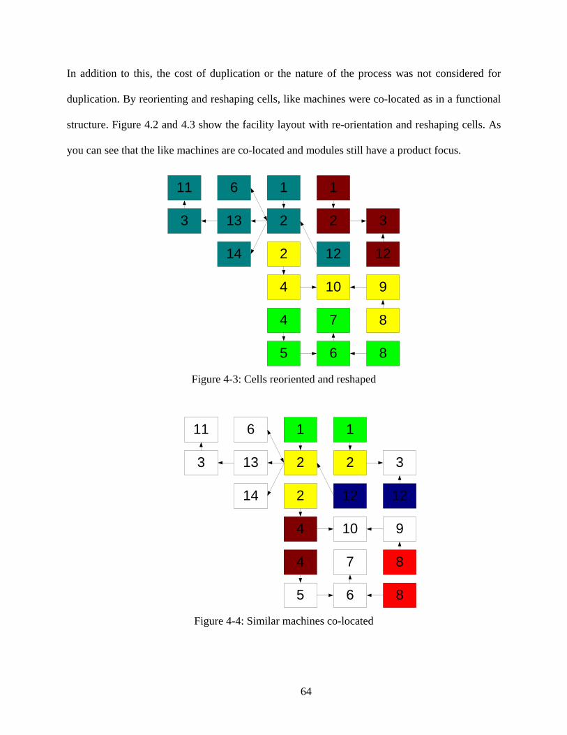
In addition to this, the cost of duplication or the nature of the process was not considered for
duplication. By reorienting and reshaping cells, like machines were co-located as in a functional
structure. Figure 4.2 and 4.3 show the facility layout with re-orientation and reshaping cells. As
you can see that the like machines are co-located and modules still have a product focus.
13
14
2
2
2
12
3
12
6
3
4
4
10
7
9
8
11 1
5
1
6 8
Figure 4-3: Cells reoriented and reshaped
13
14
2
2
2
12
3
12
6
3
4
4
10
7
9
8
11 1
5
1
6 8
Figure 4-4: Similar machines co-located
64
4.2 How R&R cells fits lean manufacturing practice
• The primary advantage of such cells relative to the group technology counterparts is that
they maintain ability to pool machine capacity by co-locating common machines that
could potentially be shared among multiple cells. This, in turn offers the following
advantages:
• Avoidance of the need to purchase additional machine capacity. This is particularly
valuable and appropriate when the shared machines are expensive.
• Capacity robustness when demand changes. With standard group technology cells with
machines under tight capacity constraints there should be a need to transfer machines
from cell to cell as demand changes. Under such a strategy, machines could remain at
fixed locations. This is particularly valuable with expensive, heavy equipment. (If
equipment is inexpensive, excess capacity and replication might be the best choice.)
• Improved ability to respond to disruptions. If a machine breaks down and a like machine
from another is adjacent, it is relatively easy to go back on line quickly.
• An opportunity to share expensive, high capacity machines among multiple cells. This
would be best under the following conditions:
o These machines have rapid changeover (ideally NOTED) and are fast cycle
relative to “takt” [2] pace of the individual cells and could essentially be put in
line in multiple cells. Robot welders might be an example of such equipment.
o The machines are “first” or “last” machines in the sequence. Parts can be batched
ahead of or after the shared process. This would create relatively little flow
65
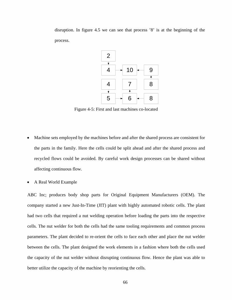
disruption. In figure 4.5 we can see that process ’8’ is at the beginning of the
process.
2
4
4
10
7
9
8
5 6 8
Figure 4-5: First and last machines co-located
• Machine sets employed by the machines before and after the shared process are consistent for
the parts in the family. Here the cells could be split ahead and after the shared process and
recycled flows could be avoided. By careful work design processes can be shared without
affecting continuous flow.
• A Real World Example
ABC Inc; produces body shop parts for Original Equipment Manufacturers (OEM). The
company started a new Just-In-Time (JIT) plant with highly automated robotic cells. The plant
had two cells that required a nut welding operation before loading the parts into the respective
cells. The nut welder for both the cells had the same tooling requirements and common process
parameters. The plant decided to re-orient the cells to face each other and place the nut welder
between the cells. The plant designed the work elements in a fashion where both the cells used
the capacity of the nut welder without disrupting continuous flow. Hence the plant was able to
better utilize the capacity of the machine by reorienting the cells.
66
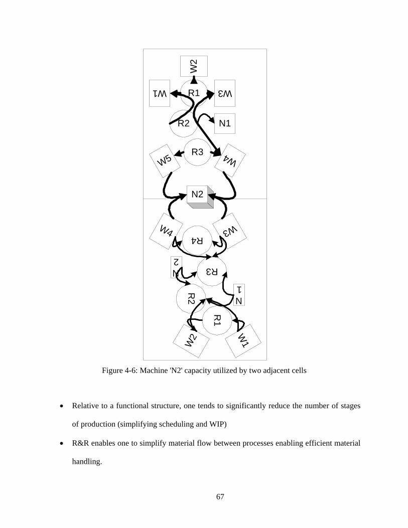
W5R3
W1 R1
R2
W4
W2
W3
N1
N2
W3R4
R3
W4
W1
R2
R1
W2
N1
N2
Figure 4-6: Machine 'N2' capacity utilized by two adjacent cells
• Relative to a functional structure, one tends to significantly reduce the number of stages
of production (simplifying scheduling and WIP)
• R&R enables one to simplify material flow between processes enabling efficient material
handling.
67
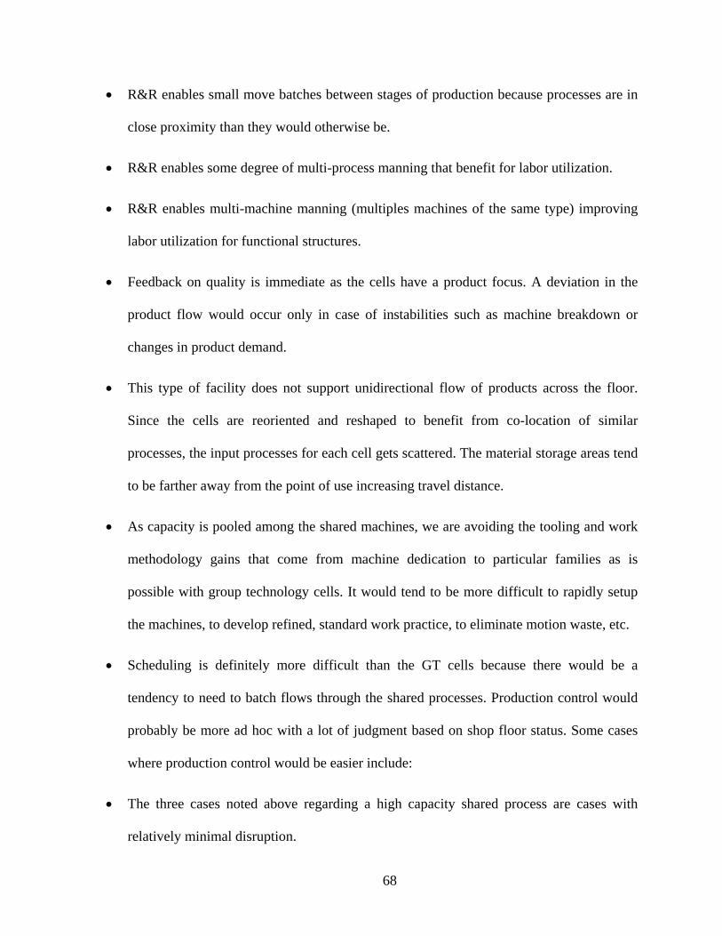
• R&R enables small move batches between stages of production because processes are in
close proximity than they would otherwise be.
• R&R enables some degree of multi-process manning that benefit for labor utilization.
• R&R enables multi-machine manning (multiples machines of the same type) improving
labor utilization for functional structures.
• Feedback on quality is immediate as the cells have a product focus. A deviation in the
product flow would occur only in case of instabilities such as machine breakdown or
changes in product demand.
• This type of facility does not support unidirectional flow of products across the floor.
Since the cells are reoriented and reshaped to benefit from co-location of similar
processes, the input processes for each cell gets scattered. The material storage areas tend
to be farther away from the point of use increasing travel distance.
• As capacity is pooled among the shared machines, we are avoiding the tooling and work
methodology gains that come from machine dedication to particular families as is
possible with group technology cells. It would tend to be more difficult to rapidly setup
the machines, to develop refined, standard work practice, to eliminate motion waste, etc.
• Scheduling is definitely more difficult than the GT cells because there would be a
tendency to need to batch flows through the shared processes. Production control would
probably be more ad hoc with a lot of judgment based on shop floor status. Some cases
where production control would be easier include:
• The three cases noted above regarding a high capacity shared process are cases with
relatively minimal disruption.
68
• When the shared process is not required by every part in both families. One cell could run
the part that needed the shared process while the other cell runs a part that does not
require the shared process
• There is no sequential flow across the floor as cell layouts have been modified to have
like machines together to better utilize its capacity. This would increase material handling
travel distance and reduces visibility on the floor.
Copyright © Mohan Swaminathan 2004
69
Chapter 5 Min-Max system
A min-max system is a material replenishment system for supplying parts to assembly and
process cells in a just-in-time basis. In designing such a system, one defines routes among
different cells in a JIT assembly plant, the timing of the routes and frequency of the run. The
approach helps to keep inventory low by capping WIP and at the same time it avoids parts
shortages. The system helps to eliminate any external impacts on the operator due to excess or
shortage of parts. By having a regular parts supply cycle, the system helps to keep logistic tasks
simple, stable and efficient. The approach helps to overcome various operational requirements or
constraints including requirements for high frequency/small quantity deliveries and limitations
on storage space on the line side.
The purpose of a min-max system is to reduce inventory on the floor and eliminate any excess or
shortage of parts. The system transports parts that are held in hand held totes from the storage
location to the cells using a routing system dependant upon cell storage capacity (i.e. how many
parts can be stored at the cell). The timing and quantity of parts to be delivered during each run is
very important to the performance of the manufacturing system. The capacity of the cell to store
parts is equivalent to the quantity in the kanban card. The supply cycle works similar to
collecting kanban cards at regular intervals. The system works similar to Kanban but does not
use a kanban card.
The routing system is a series of routes that employs milk- run strategies. With a milk-run route,
the cycle starts with replenishing containers when there is an empty space in the designated
70
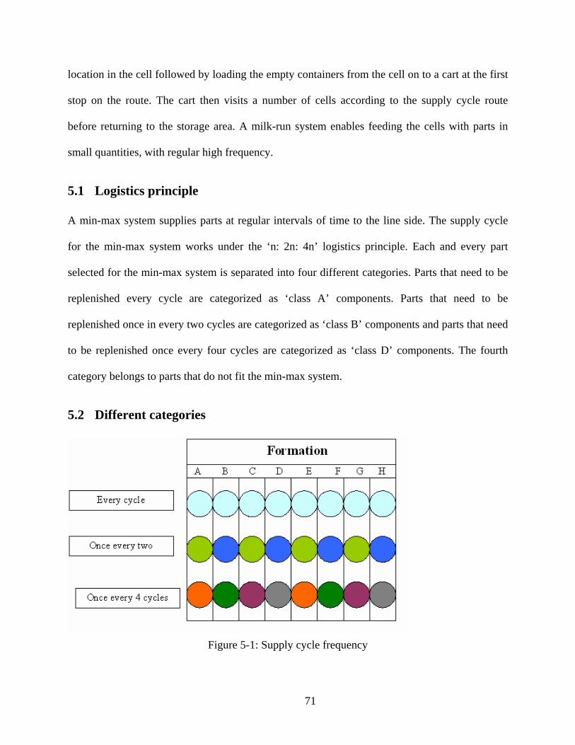
location in the cell followed by loading the empty containers from the cell on to a cart at the first
stop on the route. The cart then visits a number of cells according to the supply cycle route
before returning to the storage area. A milk-run system enables feeding the cells with parts in
small quantities, with regular high frequency.
5.1 Logistics principle A min-max system supplies parts at regular intervals of time to the line side. The supply cycle
for the min-max system works under the ‘n: 2n: 4n’ logistics principle. Each and every part
selected for the min-max system is separated into four different categories. Parts that need to be
replenished every cycle are categorized as ‘class A’ components. Parts that need to be
replenished once in every two cycles are categorized as ‘class B’ components and parts that need
to be replenished once every four cycles are categorized as ‘class D’ components. The fourth
category belongs to parts that do not fit the min-max system.
5.2 Different categories
Figure 5-1: Supply cycle frequency
71
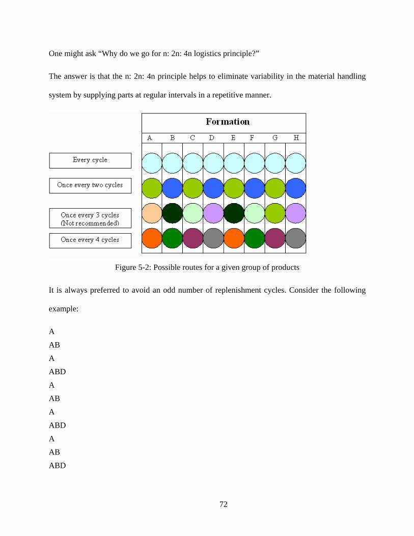
One might ask “Why do we go for n: 2n: 4n logistics principle?”
The answer is that the n: 2n: 4n principle helps to eliminate variability in the material handling
system by supplying parts at regular intervals in a repetitive manner.
Figure 5-2: Possible routes for a given group of products
It is always preferred to avoid an odd number of replenishment cycles. Consider the following
example:
A
AB
A
ABD
A
AB
A
ABD
A
AB
ABD
72
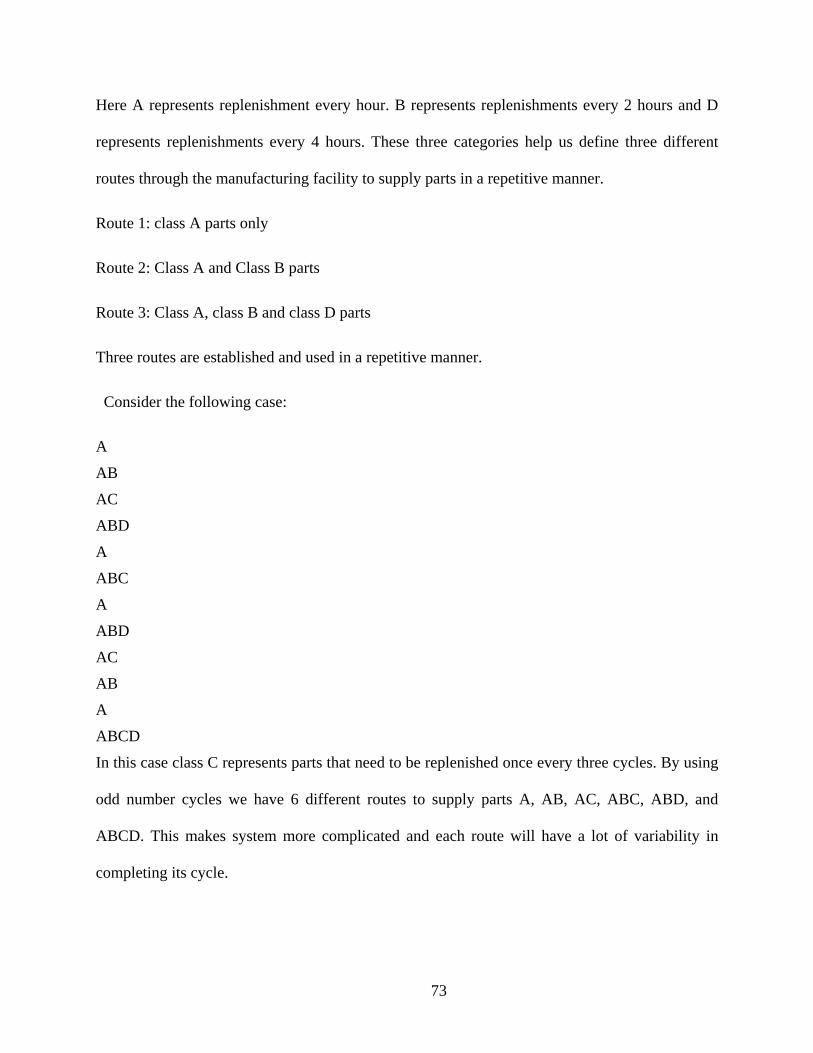
Here A represents replenishment every hour. B represents replenishments every 2 hours and D
represents replenishments every 4 hours. These three categories help us define three different
routes through the manufacturing facility to supply parts in a repetitive manner.
Route 1: class A parts only
Route 2: Class A and Class B parts
Route 3: Class A, class B and class D parts
Three routes are established and used in a repetitive manner.
Consider the following case:
A
AB
AC
ABD
A
ABC
A
ABD
AC
AB
A
ABCD
In this case class C represents parts that need to be replenished once every three cycles. By using
odd number cycles we have 6 different routes to supply parts A, AB, AC, ABC, ABD, and
ABCD. This makes system more complicated and each route will have a lot of variability in
completing its cycle.
73
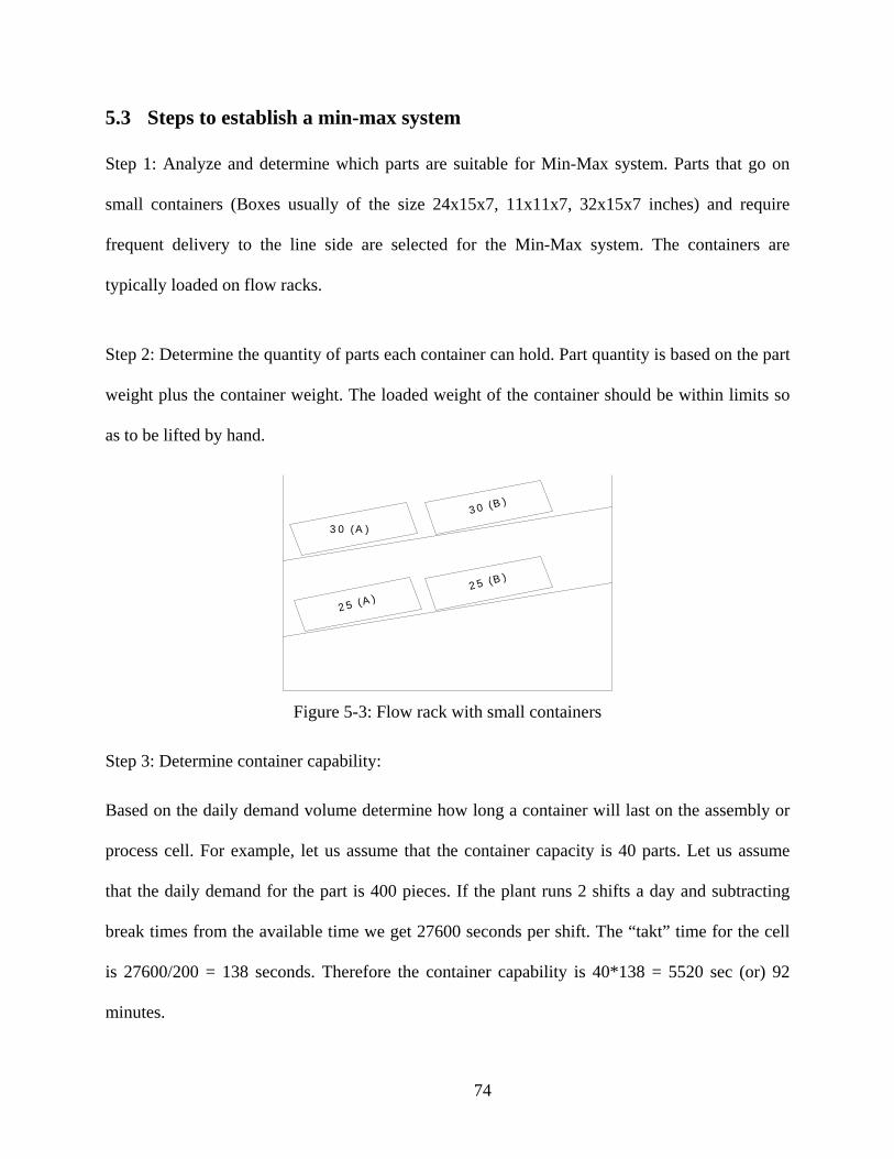
5.3 Steps to establish a min-max system Step 1: Analyze and determine which parts are suitable for Min-Max system. Parts that go on
small containers (Boxes usually of the size 24x15x7, 11x11x7, 32x15x7 inches) and require
frequent delivery to the line side are selected for the Min-Max system. The containers are
typically loaded on flow racks.
Step 2: Determine the quantity of parts each container can hold. Part quantity is based on the part
weight plus the container weight. The loaded weight of the container should be within limits so
as to be lifted by hand.
2 5 (A )
3 0 (B )
2 5 (B )
3 0 (A )
Figure 5-3: Flow rack with small containers
Step 3: Determine container capability:
Based on the daily demand volume determine how long a container will last on the assembly or
process cell. For example, let us assume that the container capacity is 40 parts. Let us assume
that the daily demand for the part is 400 pieces. If the plant runs 2 shifts a day and subtracting
break times from the available time we get 27600 seconds per shift. The “takt” time for the cell
is 27600/200 = 138 seconds. Therefore the container capability is 40*138 = 5520 sec (or) 92
minutes.
74
Step 4: Determine line side capability:
Based on available space on the flow rack and the size of the container we determine how many
containers we can have on the line side and how long it lasts.
Example:
There is space for 2 containers in the flowrack
40 pcs X 2 boxes = 80 pcs.
1 Box last 92 minutes
2 boxes X 92 = 184 min.
Therefore the line side capability is 184 min.
Once we determine the line side capability, we then have to determine the minimum number of
parts that we need to have on the line to avoid shortage of parts during the supply cycle. We use
a formula for calculating the minimum number of parts that has to be in the line at any time to
prevent shortage of parts. It is calculated using the formula {[(n-1) *no. of parts in container] +
1} where ‘n’ represents the no. of containers in the line.
Example:
Let us assume the value of ‘n’ is 2.
The no. of parts in container is 40.
The minimum number of parts on the line at any time = {[(2-1)*40] +1}
= 41 parts
75
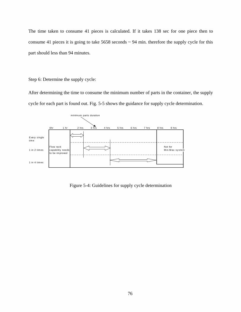
The time taken to consume 41 pieces is calculated. If it takes 138 sec for one piece then to
consume 41 pieces it is going to take 5658 seconds ~ 94 min. therefore the supply cycle for this
part should less than 94 minutes.
Step 6: Determine the supply cycle:
After determining the time to consume the minimum number of parts in the container, the supply
cycle for each part is found out. Fig. 5-5 shows the guidance for supply cycle determination.
m inim um parts duration
0hr 1 hr 2 hrs 3 hrs 4 hrs 5 hrs 6 hrs 7 hrs 8 hrs 9 hrs
E very s ingletim e
Flow rack Not for 1 in 2 t im es capability needs M in-M ax sys tem
to be im proved
1 in 4 t im es
Figure 5-4: Guidelines for supply cycle determination
76
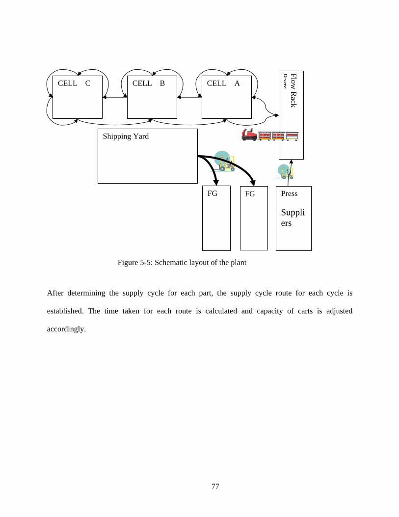
CELL C CELL B CELL A
Flow R
ack Parts
Shipping Yard
FG Press Suppliers
FG
Figure 5-5: Schematic layout of the plant
After determining the supply cycle for each part, the supply cycle route for each cycle is
established. The time taken for each route is calculated and capacity of carts is adjusted
accordingly.
77
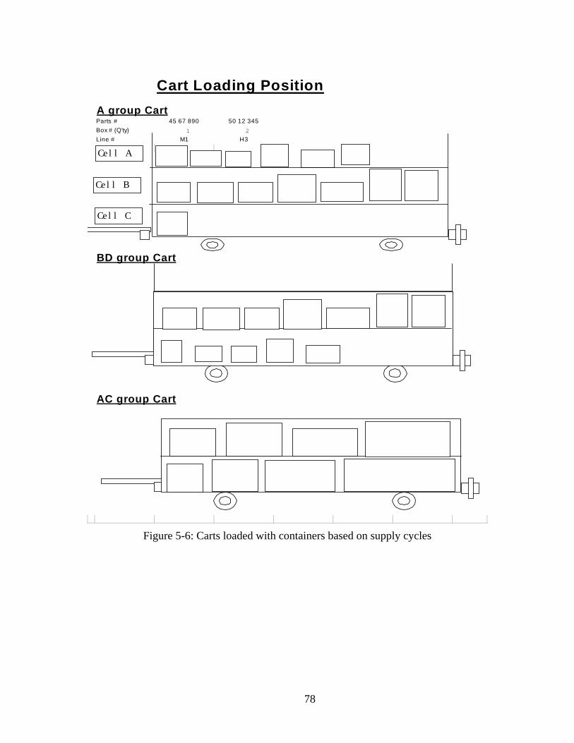
Cart Loading PositionA group CartParts # 45 67 890 50 12 345Box # (Q'ty) 1 2Line # M1 H3
BD group Cart
AC group Cart
Ce l l B
Ce l l A
Ce l l C
Figure 5-6: Carts loaded with containers based on supply cycles
78
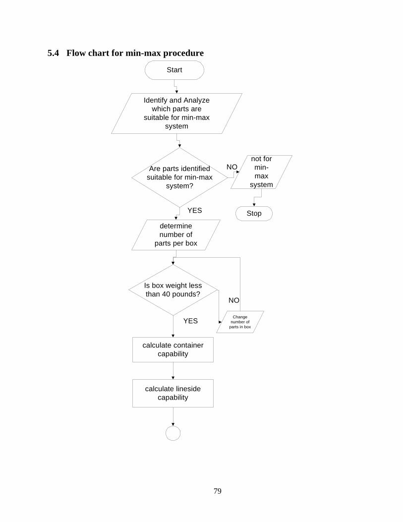
5.4 Flow chart for min-max procedure
Start
Identify and Analyzewhich parts are
suitable for min-maxsystem
Are parts identifiedsuitable for min-max
system?
determinenumber of
parts per box
Is box weight lessthan 40 pounds?
calculate containercapability
YES
YES
not formin-max
system
Stop
Changenumber of
parts in box
NO
NO
calculate linesidecapability
79
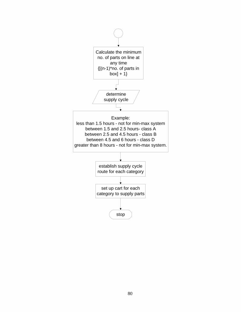
determinesupply cycle
Example:less than 1.5 hours - not for min-max system
between 1.5 and 2.5 hours- class Abetween 2.5 and 4.5 hours - class Bbetween 4.5 and 6 hours - class D
greater than 8 hours - not for min-max system.
establish supply cycleroute for each category
set up cart for eachcategory to supply parts
stop
Calculate the minimumno. of parts on line at
any time{[(n-1)*no. of parts in
box] + 1}
80
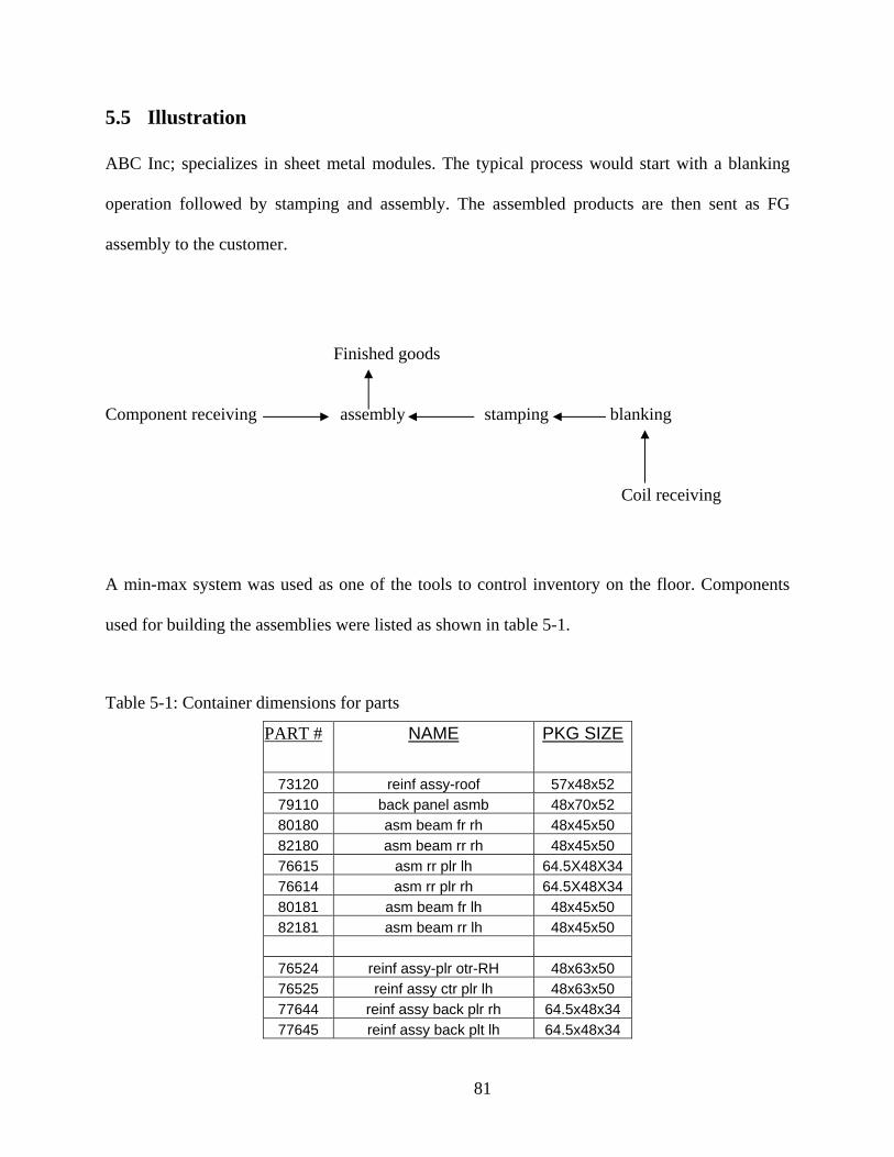
5.5 Illustration ABC Inc; specializes in sheet metal modules. The typical process would start with a blanking
operation followed by stamping and assembly. The assembled products are then sent as FG
assembly to the customer.
Finished goods Component receiving assembly stamping blanking
Coil receiving
A min-max system was used as one of the tools to control inventory on the floor. Components
used for building the assemblies were listed as shown in table 5-1.
Table 5-1: Container dimensions for parts
PART # NAME PKG SIZE
73120 reinf assy-roof 57x48x52 79110 back panel asmb 48x70x52 80180 asm beam fr rh 48x45x50 82180 asm beam rr rh 48x45x50 76615 asm rr plr lh 64.5X48X34 76614 asm rr plr rh 64.5X48X34 80181 asm beam fr lh 48x45x50 82181 asm beam rr lh 48x45x50
76524 reinf assy-plr otr-RH 48x63x50 76525 reinf assy ctr plr lh 48x63x50 77644 reinf assy back plr rh 64.5x48x34 77645 reinf assy back plt lh 64.5x48x34
81
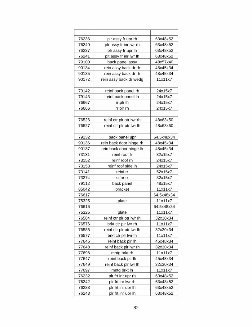
76236 plr assy fr upr rh 63x48x52 76240 plr assy fr inr lwr rh 63x48x52 76237 plr assy fr upr lh 63x48x52 76241 plt assy fr inr lwr lh 63x48x52 79100 back panel assy 48x57x40 90134 rein assy back dr rh 48x45x34 90135 rein assy back dr rh 48x45x34 90172 rein assy back dr wedg 11x11x7
79142 reinf back panel rh 24x15x7 79143 reinf back panel lh 24x15x7 76667 rr plr lh 24x15x7 76666 rr plr rh 24x15x7
76526 reinf ctr plr otr lwr rh 48x63x50 76527 reinf ctr plr otr lwr lh 48x63x50
79132 back panel upr 64.5x48x34 90136 rein back door hinge rh 48x45x34 90137 rein back door hinge lh 48x45x34 73131 reinf roof fr 32x15x7 73152 reinf roof rh 24x15x7 73153 reinf roof side lh 24x15x7 73141 reinf rr 52x15x7 73274 stfnr rr 32x15x7 79112 back panel 48x15x7 85042 bracket 11x11x7 76617 64.5x48x34 75325 plate 11x11x7 76616 64.5x48x34 75325 plate 11x11x7 76584 reinf ctr plr otr lwr rh 32x30x34 76576 brkt ctr plr lwr rh 11x11x7 76585 reinf ctr plr otr lwr lh 32x30x34 76577 brkt ctr plr lwr lh 11x11x7 77646 reinf back plr rh 45x48x34 77648 reinf back plr lwr rh 32x30x34 77696 mntg brkt rh 11x11x7 77647 reinf back plr lh 45x48x34 77649 reinf back plr lwr lh 32x30x34 77697 mntg brkt lh 11x11x7 76232 plr frt inr upr rh 63x48x52 76242 plr frt inr lwr rh 63x48x52 76233 plr frt inr upr lh 63x48x52 76243 plr frt inr upr lh 63x48x52
82
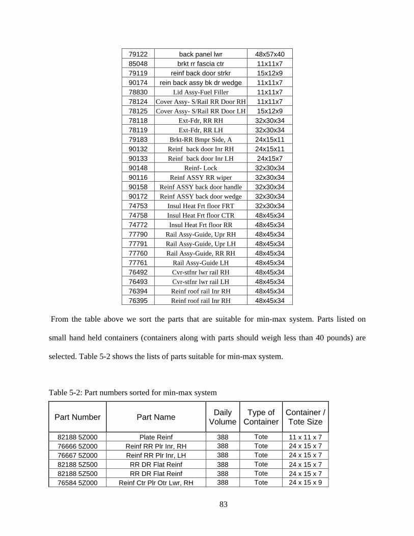
79122 back panel lwr 48x57x40 85048 brkt rr fascia ctr 11x11x7 79119 reinf back door strkr 15x12x9 90174 rein back assy bk dr wedge 11x11x7 78830 Lid Assy-Fuel Filler 11x11x7 78124 Cover Assy- S/Rail RR Door RH 11x11x7 78125 Cover Assy- S/Rail RR Door LH 15x12x9 78118 Ext-Fdr, RR RH 32x30x34 78119 Ext-Fdr, RR LH 32x30x34 79183 Brkt-RR Bmpr Side, A 24x15x11 90132 Reinf back door Inr RH 24x15x11 90133 Reinf back door Inr LH 24x15x7 90148 Reinf- Lock 32x30x34 90116 Reinf ASSY RR wiper 32x30x34 90158 Reinf ASSY back door handle 32x30x34 90172 Reinf ASSY back door wedge 32x30x34 74753 Insul Heat Frt floor FRT 32x30x34 74758 Insul Heat Frt floor CTR 48x45x34 74772 Insul Heat Frt floor RR 48x45x34 77790 Rail Assy-Guide, Upr RH 48x45x34 77791 Rail Assy-Guide, Upr LH 48x45x34 77760 Rail Assy-Guide, RR RH 48x45x34 77761 Rail Assy-Guide LH 48x45x34 76492 Cvr-stfnr lwr rail RH 48x45x34 76493 Cvr-stfnr lwr rail LH 48x45x34 76394 Reinf roof rail Inr RH 48x45x34 76395 Reinf roof rail Inr RH 48x45x34
From the table above we sort the parts that are suitable for min-max system. Parts listed on
small hand held containers (containers along with parts should weigh less than 40 pounds) are
selected. Table 5-2 shows the lists of parts suitable for min-max system.
Table 5-2: Part numbers sorted for min-max system
Part Number Part Name Daily Volume
Type of Container
Container / Tote Size
82188 5Z000 Plate Reinf 388 Tote 11 x 11 x 7 76666 5Z000 Reinf RR Plr Inr, RH 388 Tote 24 x 15 x 7 76667 5Z000 Reinf RR Plr Inr, LH 388 Tote 24 x 15 x 7 82188 5Z500 RR DR Flat Reinf 388 Tote 24 x 15 x 7 82188 5Z500 RR DR Flat Reinf 388 Tote 24 x 15 x 7 76584 5Z000 Reinf Ctr Plr Otr Lwr, RH 388 Tote 24 x 15 x 9
83
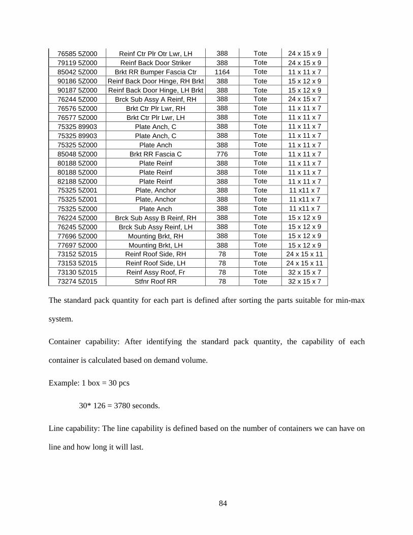
76585 5Z000 Reinf Ctr Plr Otr Lwr, LH 388 Tote 24 x 15 x 9 79119 5Z000 Reinf Back Door Striker 388 Tote 24 x 15 x 9 85042 5Z000 Brkt RR Bumper Fascia Ctr 1164 Tote 11 x 11 x 7 90186 5Z000 Reinf Back Door Hinge, RH Brkt 388 Tote 15 x 12 x 9 90187 5Z000 Reinf Back Door Hinge, LH Brkt 388 Tote 15 x 12 x 9 76244 5Z000 Brck Sub Assy A Reinf, RH 388 Tote 24 x 15 x 7 76576 5Z000 Brkt Ctr Plr Lwr, RH 388 Tote 11 x 11 x 7 76577 5Z000 Brkt Ctr Plr Lwr, LH 388 Tote 11 x 11 x 7 75325 89903 Plate Anch, C 388 Tote 11 x 11 x 7 75325 89903 Plate Anch, C 388 Tote 11 x 11 x 7 75325 5Z000 Plate Anch 388 Tote 11 x 11 x 7 85048 5Z000 Brkt RR Fascia C 776 Tote 11 x 11 x 7 80188 5Z000 Plate Reinf 388 Tote 11 x 11 x 7 80188 5Z000 Plate Reinf 388 Tote 11 x 11 x 7 82188 5Z000 Plate Reinf 388 Tote 11 x 11 x 7 75325 5Z001 Plate, Anchor 388 Tote 11 x11 x 7 75325 5Z001 Plate, Anchor 388 Tote 11 x11 x 7 75325 5Z000 Plate Anch 388 Tote 11 x11 x 7 76224 5Z000 Brck Sub Assy B Reinf, RH 388 Tote 15 x 12 x 9 76245 5Z000 Brck Sub Assy Reinf, LH 388 Tote 15 x 12 x 9 77696 5Z000 Mounting Brkt, RH 388 Tote 15 x 12 x 9 77697 5Z000 Mounting Brkt, LH 388 Tote 15 x 12 x 9 73152 5Z015 Reinf Roof Side, RH 78 Tote 24 x 15 x 11 73153 5Z015 Reinf Roof Side, LH 78 Tote 24 x 15 x 11 73130 5Z015 Reinf Assy Roof, Fr 78 Tote 32 x 15 x 7 73274 5Z015 Stfnr Roof RR 78 Tote 32 x 15 x 7
The standard pack quantity for each part is defined after sorting the parts suitable for min-max
system.
Container capability: After identifying the standard pack quantity, the capability of each
container is calculated based on demand volume.
Example: 1 box = 30 pcs
30* 126 = 3780 seconds.
Line capability: The line capability is defined based on the number of containers we can have on
line and how long it will last.
84
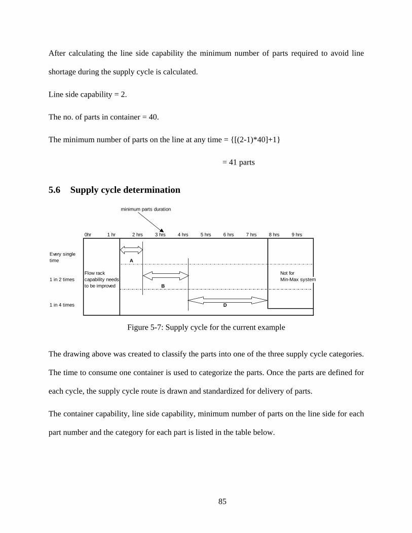
After calculating the line side capability the minimum number of parts required to avoid line
shortage during the supply cycle is calculated.
Line side capability = 2.
The no. of parts in container = 40.
The minimum number of parts on the line at any time = {[(2-1)*40]+1}
= 41 parts
5.6 Supply cycle determination
minimum parts duration
0hr 1 hr 2 hrs 3 hrs 4 hrs 5 hrs 6 hrs 7 hrs 8 hrs 9 hrs
Every singletime
Flow rack Not for 1 in 2 times capability needs Min-Max system
to be improved B
1 in 4 times D
A
Figure 5-7: Supply cycle for the current example
The drawing above was created to classify the parts into one of the three supply cycle categories.
The time to consume one container is used to categorize the parts. Once the parts are defined for
each cycle, the supply cycle route is drawn and standardized for delivery of parts.
The container capability, line side capability, minimum number of parts on the line side for each
part number and the category for each part is listed in the table below.
85
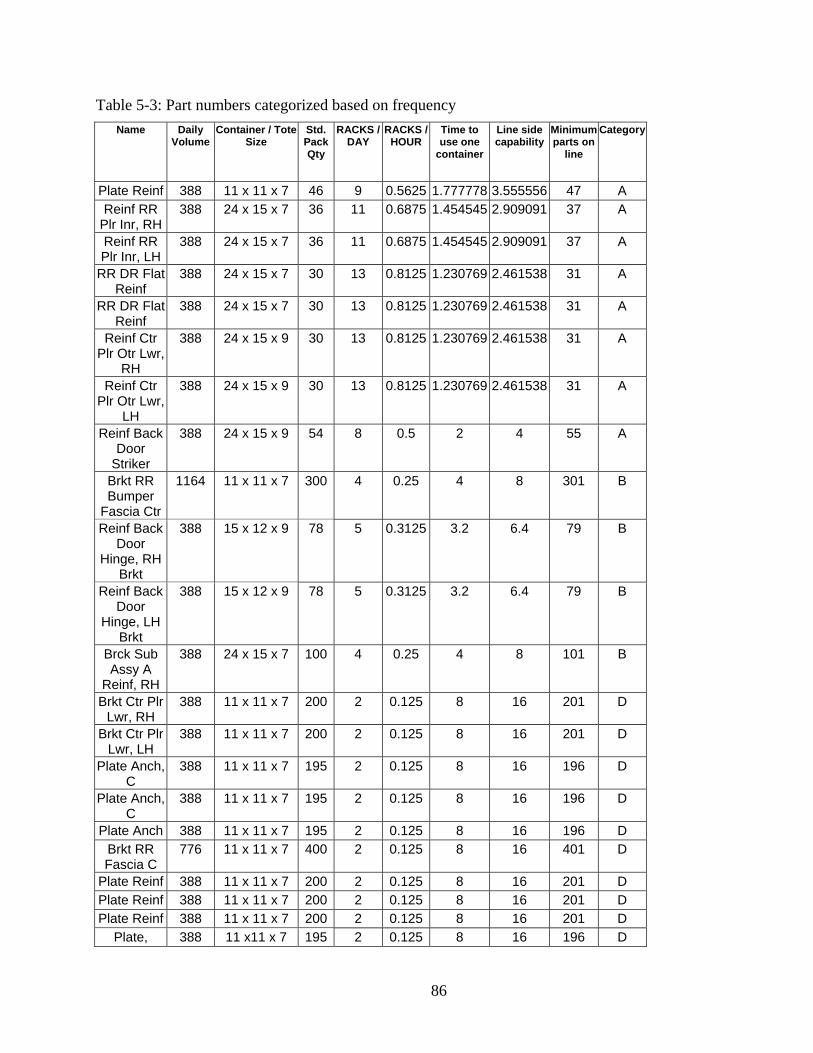
Table 5-3: Part numbers categorized based on frequency Name Daily
Volume Container / Tote
Size Std. Pack Qty
RACKS / DAY
RACKS / HOUR
Time to use one
container
Line side capability
Minimum parts on
line
Category
Plate Reinf 388 11 x 11 x 7 46 9 0.5625 1.777778 3.555556 47 A Reinf RR
Plr Inr, RH 388 24 x 15 x 7 36 11 0.6875 1.454545 2.909091 37 A
Reinf RR Plr Inr, LH
388 24 x 15 x 7 36 11 0.6875 1.454545 2.909091 37 A
RR DR Flat Reinf
388 24 x 15 x 7 30 13 0.8125 1.230769 2.461538 31 A
RR DR Flat Reinf
388 24 x 15 x 7 30 13 0.8125 1.230769 2.461538 31 A
Reinf Ctr Plr Otr Lwr,
RH
388 24 x 15 x 9 30 13 0.8125 1.230769 2.461538 31 A
Reinf Ctr Plr Otr Lwr,
LH
388 24 x 15 x 9 30 13 0.8125 1.230769 2.461538 31 A
Reinf Back Door
Striker
388 24 x 15 x 9 54 8 0.5 2 4 55 A
Brkt RR Bumper
Fascia Ctr
1164 11 x 11 x 7 300 4 0.25 4 8 301 B
Reinf Back Door
Hinge, RH Brkt
388 15 x 12 x 9 78 5 0.3125 3.2 6.4 79 B
Reinf Back Door
Hinge, LH Brkt
388 15 x 12 x 9 78 5 0.3125 3.2 6.4 79 B
Brck Sub Assy A
Reinf, RH
388 24 x 15 x 7 100 4 0.25 4 8 101 B
Brkt Ctr Plr Lwr, RH
388 11 x 11 x 7 200 2 0.125 8 16 201 D
Brkt Ctr Plr Lwr, LH
388 11 x 11 x 7 200 2 0.125 8 16 201 D
Plate Anch, C
388 11 x 11 x 7 195 2 0.125 8 16 196 D
Plate Anch, C
388 11 x 11 x 7 195 2 0.125 8 16 196 D
Plate Anch 388 11 x 11 x 7 195 2 0.125 8 16 196 D Brkt RR Fascia C
776 11 x 11 x 7 400 2 0.125 8 16 401 D
Plate Reinf 388 11 x 11 x 7 200 2 0.125 8 16 201 D Plate Reinf 388 11 x 11 x 7 200 2 0.125 8 16 201 D Plate Reinf 388 11 x 11 x 7 200 2 0.125 8 16 201 D
Plate, 388 11 x11 x 7 195 2 0.125 8 16 196 D
86
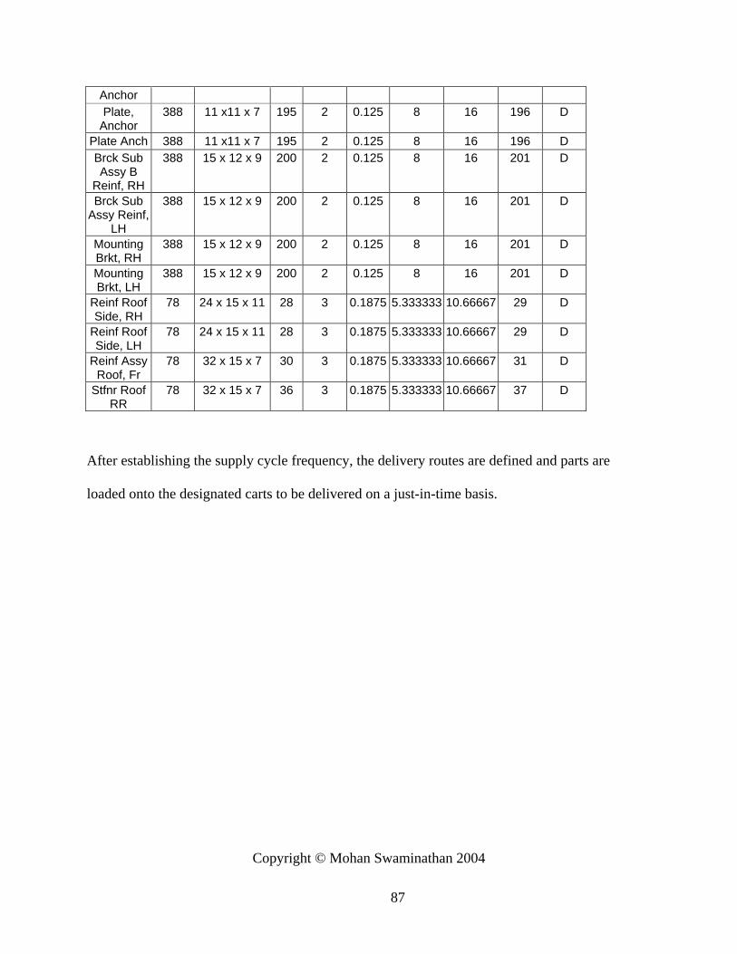
Anchor Plate,
Anchor 388 11 x11 x 7 195 2 0.125 8 16 196 D
Plate Anch 388 11 x11 x 7 195 2 0.125 8 16 196 D Brck Sub Assy B
Reinf, RH
388 15 x 12 x 9 200 2 0.125 8 16 201 D
Brck Sub Assy Reinf,
LH
388 15 x 12 x 9 200 2 0.125 8 16 201 D
Mounting Brkt, RH
388 15 x 12 x 9 200 2 0.125 8 16 201 D
Mounting Brkt, LH
388 15 x 12 x 9 200 2 0.125 8 16 201 D
Reinf Roof Side, RH
78 24 x 15 x 11 28 3 0.1875 5.333333 10.66667 29 D
Reinf Roof Side, LH
78 24 x 15 x 11 28 3 0.1875 5.333333 10.66667 29 D
Reinf Assy Roof, Fr
78 32 x 15 x 7 30 3 0.1875 5.333333 10.66667 31 D
Stfnr Roof RR
78 32 x 15 x 7 36 3 0.1875 5.333333 10.66667 37 D
After establishing the supply cycle frequency, the delivery routes are defined and parts are
loaded onto the designated carts to be delivered on a just-in-time basis.
Copyright © Mohan Swaminathan 2004
87
Chapter 6 Conclusions
6.1 Summary
This research highlighted the importance of plant layout and material handling in promoting lean
manufacturing on the shop floor. Chapter 2 provides a brief overview of the existing procedure
for forming hybrid cellular constructs using layout modules. The procedure was studied in the
context of lean and the limitations were presented. The existing procedure was followed by a
modified procedure for forming hybrid cellular constructs characterized by layout modules. The
effectiveness of the modified procedure was studied by comparing the number of duplicates
required for each process to run a facility designed under different methodologies. The modified
procedure was then applied to form the hybrid cellular constructs specifically, hybrid flow shop
layout and reoriented & reshaped cells.
The following chapters clearly describe the hybrid cellular constructs in terms of their key
features, structure and mode of operation. This thesis then defines the lean practices that are
compatible with each construct and highlights those that are incompatible. It suggests how to
modify lean practices to fit and at least obtain some benefits. A real world case study was used to
study the applicability of lean under each construct.
A good layout and a good material flow should always be augmented with some good materials
management system. This thesis proposes a design methodology of such a materials management
system for supplying parts in a just-in-time basis.
88
6.2 Future Research
Although the modified procedure for forming hybrid cellular constructs using layout modules
proved to be successful under the given case study, it still needs to be tested under different
manufacturing circumstances. In particular, the modules are formed based on the frequency of
occurrence of common sub-string. If the frequency of sub-strings changes the nucleus of the
module can change which will then affect the overall flow and this is a technical issue worthy to
address.
The hybrid cellular constructs in question improve flow and machine capacity. But these
constructs pose greater problem in terms of production control system. An extension of this
research would be to develop a production control system that would best fit the different
constructs in question.
The thesis focused on studying only two different hybrid cellular constructs. Other constructs
like virtual manufacturing cells and cascading cells can also be studied in detail in terms of lean
practices and their applicability to various manufacturing environments.
Copyright © Mohan Swaminathan 2004
89
REFERENCES:
1 . Womack and Jones, Lean thinking, 1999, Lean Enterprise Institute.
2 . Jon C. Yingling, Course Notes – Principles and Practices of Lean Manufacturing, 2001,
University of Kentucky, Lexington, KY.
3. Suzaki, K. (1987). The new manufacturing challenge: Techniques for continuous
improvement. New York, NY: Free Press.
4. Tompkins, J. & White, J., 1984, Facilities Planning. New Tork, NY: John Wiley.
5. Gallagher, C.C. & Knight, W.A. (1973). Group Technology. London, UK: Butterworths
Group.
6 . Burbidge, J.L. (1963, June). “Production flow Analysis”. Production Engineer.
7. King, J.R. 1980, Machine-Component grouping in production flow analysis: An approach
using rank order clustering algorithm, Internal Journal of Production Research, Vol. 18(2), pp
213-232.
8. Anderberg, M.R, 1973, Cluster Analysis for Applications, Academic Press, New York, NY.
9. Irani, S.A. (1990). A Flow Decomposition Aproach for Integrated Layout Design of Virtual
group Technology Flowlines. Ph.D. Dissertation, Department of Industrial and Manufacturing
Engineering, the Pennsylvania State University, College Park, PA.
10. Mike Rother & Rick Harris (2001), Creating Continuous Flow, Lean Enterprise Institute
11. Irani, S.A. & Huang, H (2000), Custom Design of Facility Layouts for Multi-Product
Facilities using Layout Modules, IEEE transactions on Robotics and Automation, 16(3), 259-
267.
90
12. Narayanan, M. (2002), Hybrid Flow Strategies for high variety low volume manufacturing
facilities to implement flow and pull, Masters of Science thesis, department of Manufacturing
Systems Engineering, the University of Kentucky, Lexington, KY.
13. Wallace J, Hopp and Mark L. Spearman, 2001, Factory Physics, Irwin McGraw Hill.
14. Shukla, J, 1995, Hybrid and Progressive Layouts for Cellular Jobshops, Masters of Science
thesis, Department of Mechanical Engineering, University of Minnesota, Minneapolis, MN.
91
VITA
Mohan Swaminathan was born in Madras, India on 31st December 1978. He earned his
high school diploma from Madras, India in 1996. He earned his Bachelor’s degree with
honors in the field of Mechanical Engineering from the University of Madras, India in
2000. He joined the Masters program in Manufacturing Systems Engineering at the
University of Kentucky in fall semester of 2000. He worked as a Research Assistant
under Dr. Jon C. Yingling and Dr. Janet Lumpp at the Center for Robotics and
Manufacturing Systems during his Masters degree.
92