contributions to the development of microgrids: aggregated

University of Wollongong University of Wollongong

Research Online Research Online

University of Wollongong Thesis Collection 1954-2016 University of Wollongong Thesis Collections

2015

Contributions to the development of microgrids: Aggregated modelling and Contributions to the development of microgrids: Aggregated modelling and

operational aspects operational aspects

Athmi Vidarshika Jayawardena University of Wollongong, [email protected]

Follow this and additional works at: https://ro.uow.edu.au/theses

University of Wollongong University of Wollongong

Copyright Warning Copyright Warning

You may print or download ONE copy of this document for the purpose of your own research or study. The University

does not authorise you to copy, communicate or otherwise make available electronically to any other person any

copyright material contained on this site.

You are reminded of the following: This work is copyright. Apart from any use permitted under the Copyright Act

1968, no part of this work may be reproduced by any process, nor may any other exclusive right be exercised,

without the permission of the author. Copyright owners are entitled to take legal action against persons who infringe

their copyright. A reproduction of material that is protected by copyright may be a copyright infringement. A court

may impose penalties and award damages in relation to offences and infringements relating to copyright material.

Higher penalties may apply, and higher damages may be awarded, for offences and infringements involving the

conversion of material into digital or electronic form.

Unless otherwise indicated, the views expressed in this thesis are those of the author and do not necessarily Unless otherwise indicated, the views expressed in this thesis are those of the author and do not necessarily

represent the views of the University of Wollongong. represent the views of the University of Wollongong.

Recommended Citation Recommended Citation Jayawardena, Athmi Vidarshika, Contributions to the development of microgrids: Aggregated modelling and operational aspects, Doctor of Philosophy thesis, School of Electrical, Computer and Telecommunications Engineering, University of Wollongong, 2015. https://ro.uow.edu.au/theses/4447

Research Online is the open access institutional repository for the University of Wollongong. For further information contact the UOW Library: [email protected]

https://ro.uow.edu.au/

https://ro.uow.edu.au/theses

https://ro.uow.edu.au/theses

https://ro.uow.edu.au/thesesuow

https://ro.uow.edu.au/theses?utm_source=ro.uow.edu.au%2Ftheses%2F4447&utm_medium=PDF&utm_campaign=PDFCoverPages

School of Electrical, Computer and Telecommunications Engineering

Contributions to the Development of Microgrids:

Aggregated Modelling and Operational Aspects

Athmi Vidarshika Jayawardena, BSc(Eng)

Supervisors

Dr. Lasantha Meegahapola, Dr. Duane Robinson & Prof. Sarath Perera

This thesis is presented as part of the requirements for the

Award of the Degree of

Doctor of Philosophy

of the

University of Wollongong

March 2015

Dedicated to my parents...

Certification

I, Athmi Vidarshika Jayawardena, declare that this thesis, submitted in fulfilment of

the requirements for the award of Doctor of Philosophy, in the School of Electrical,

Computer and Telecommunications Engineering, University of Wollongong, is en-

tirely my own work unless otherwise referenced or acknowledged. This manuscript

has not been submitted for qualifications at any other academic institute.

Athmi Vidarshika Jayawardena

Date: 08 March 2015

ii

Abstract

Increasing levels of penetration of distributed energy resources (DERs) have trans-

formed distribution networks from passive to active networks and introduced the

concept of microgrids. Dynamic characteristics of microgrids operating either in

grid connected or islanded modes can be different from the traditional distribution

networks due to the combination of different DERs. In order to make microgrid

operation attractive, the issues associated with microgrids need to be properly anal-

ysed. This thesis examines the modelling of microgrids and investigates different

aspects of their operation.

In the first phase of the work presented in this thesis, dynamic characteristics of

microgrids comprising different distributed generators are investigated. The impor-

tance of understanding the dynamic behaviour of microgrids is highlighted through

a comparative analysis carried out on a hybrid microgrid. A simulation model of a

hybrid microgrid comprising a PV system, a doubly-fed induction generator (DFIG)

based wind power plant, a mini hydro power plant, and loads is developed for the

analysis. This study revealed that the dynamic characteristics of the microgrid are

significantly influenced by the characteristics of individual DERs and their control

systems. It has been noted that during grid connected mode, features of the external

grid also have an impact on microgrid behaviour.

The second phase of this thesis is focused on aggregated modelling of grid con-

nected microgrids comprising both inverter interfaced and non-inverter interfaced

DERs. For stability analysis, the common practice is to separate the power sys-

tem into a study area of interest and external areas. In general, the study area is

represented in a detailed manner while external areas are represented by dynamic

equivalents. This thesis investigates the applicability of modal analysis as a tool for

dynamic model equivalencing of grid connected hybrid microgrids while introducing

a new index to identify the dominant modes of the system. The grid connected

microgrid is represented as a single dynamic device while retaining the important

iii

dynamics. Linearised models of different DERs with control systems and loads are

developed for this study. Several case studies are carried out to validate the re-

duced order dynamic model of the microgrid by testing under different operating

conditions. Furthermore, the model equivalencing is applied on microgrids in a

multi-microgrid environment to validate the methodology.

Similar to the large generators in conventional power systems, grid connected

microgrids have the potential to participate in energy markets to achieve technical,

financial and environmental benefits. In order to enable such operation, a systematic

approach in developing a capability tool for a grid connected microgrid is presented

in the next phase of this thesis. A grid connected microgrid can be viewed as a single

generator or a load depending on power import or export at the grid supply point.

However, unlike in a single generator with simple machine limitations, active and

reactive power transfer limits of a grid connected microgrid depend on many factors,

including different and multiple machine capability limits, local load demands, and

distribution line capacities. A mathematical model is developed to establish the

active and reactive power transfer capability at the point of common coupling, con-

sidering all aspects of grid connected microgrids. Capability diagrams for different

microgrid scenarios are derived using the mathematical model, and the applicability

of microgrid capability diagram as a tool in the energy market operation is also

presented.

The low voltage ride through (LVRT) capability of grid connected microgrids and

the potential to provide voltage support as an ancillary service for the main grid are

investigated in the final phase of the thesis. Two approaches are followed to inves-

tigate the LVRT capability of a microgrid as a single entity. In the first approach,

dynamic voltage support at the microgrid point of common coupling is improved by

using a distribution static synchronous compensator (DSTATCOM) connected to

the low voltage side of the distribution transformer of the microgrid. The collective

effect of the LVRT capabilities of the distributed generators in the microgrid is used

to provide voltage and reactive power support to the external grid in the second

iv

approach. Furthermore, operation of the DSTATCOM in multi-microgrid environ-

ment and islanded mode are also investigated under different operating conditions.

Impact of the DSTATCOM location in the microgrid is also analysed by installing it

at the low voltage side of the microgrid distribution transformer, at distributed gen-

erator terminals and at the bus bar with lowest reactive power margin. Variations

of the microgrid system parameters during the fault and after fault clearance are

analysed to identify the most appropriate location for DSTATCOM operation. It

was identified that having the DSTATCOM at the low voltage side of the microgrid

distribution transformer is far more beneficial in situations of microgrid transition

from grid connected to islanded mode of operation, which would improve the mi-

crogrid voltage profile. DSTATCOM operation would reduce the reactive power

demand from the external grid which arises due to faults in microgrids containing

mains connected induction motor loads.

Based on the studies presented in this thesis, it can be identified that integration

of multiple microgrids into the utility grid will allow the microgrids to provide ancil-

lary services to the main grid during grid connected mode, and provide emergency

services to adjacent microgrids during a utility grid outage. The work presented in

this thesis provides the groundwork which will enable microgrids to perform such

ancillary services.

v

Acknowledgements

I wish to express my sincere appreciation to many people who have helped me

throughout my PhD candidature at the University of Wollongong.

I wish to thank my supervising team Dr Lasantha Meegahapola, Dr Duane

Robinson and Professor Sarath Perera for the valuable guidance and encourage-

ment given throughout my studies. I wish to particularly thank Professor Sarath

Perera for providing me the opportunity to pursue postgraduate studies at the Uni-

versity of Wollongong and the support given throughout the study period in many

ways.

The personal and administrative support provided by Jacqueline Adriaanse,

Sasha Nikolic, Roslyn Causer-Temby, and all the Technical Staff of School of Elec-

trical, Computer and Telecommunications Engineering, University of Wollongong

are acknowledged with gratitude.

I would like to thank Dr Upuli Jayatunga, and my colleagues Brian Perera,

Malithi Gunawardana, Amila Wickramasinghe, Dothinka Ranamuka and Kanchana

Amarasekara for their support given during my stay in Wollongong.

Special thanks go to my uncle, Ananda Jayawardana and aunt Champa Jayawar-

dana for supporting me in numerous ways during my candidature.

Last but not least, my heartiest gratitude goes to my parents, Upali Jayawar-

dena and Malathie Fernando, my husband, Devinda Perera, my sister, Savidya and

brother-in-law, Hirulak for their unconditional love and continuous support. Thank

you so much for your endless love, encouragement, guidance and all the sacrifices

you made on behalf of me to come this far. I would not have been able to complete

this thesis without you.

vi

List of Principal Symbols and Abbreviations

ADNC active distribution network cell

ANN artificial neural network

AVR automatic voltage regulator

CCT critical clearing time

CHP combined heat and power

DER distributed energy resources

DFIG doubly-fed induction generator

DG distributed generator

DNSP distribution network service provider

DSL DIgSILENT simulation language

DSTATCOM distribution static synchronous compensator

GHG greenhouse gas

GSP grid supply point

HV high voltage

HVDC high voltage direct current

IM induction motor

LV low voltage

LVRT low voltage ride through

MC microsource controller

MCC microgrid central controller

MG microgrid

MHPP mini-hydro power plant

MPPT maximum power point tracking

MV medium voltage

ODE ordinary differential equation

PCC point of common coupling

p.f. power factor

PHEV plug-in hybrid electric vehicle

PLL phase locked loop

PMS power management strategies

pu per unit

PV photovoltaic

vii

ROCOF rate of change of frequency

SCC short circuit capacity

SG synchronous generator

SMA selective modal analysis

SME synchronic model equivalencing

V2G vehicle-to-grid

VR voltage regulation

VSI voltage source inverter

WTG wind turbine generator

A system matrix

α exponent of the static load active power

β exponent of the static load reactive power

Cdc storage capacitance

Cir center of the circle defining DFIG rotor current limitation

Cis center of the circle defining DFIG stator current limitation

Co/p output coefficient matrix

D −Q dq axis of the global reference frame

δi angle between the d-axis of the global reference frame and the

d-axis of the local reference frame corresponding to the ith

dynamic device

∆iDGi variation of output current of the ith DG

∆Idi, ∆Iqi variation of the dq axes currents of the ith dynamic device in the

local reference frame

∆IDi, ∆IQi variation of the dq axes currents of the ith dynamic device in the

global reference frame

∆Ipcc variation of the current vector through the microgrid pcc

∆ωi variation of angular frequency of the ith local dq reference frame

∆vDGi variation of the terminal voltage of the ith DG

∆V di, ∆Vqi variation of the dq axes voltages of the ith dynamic device in the

local reference frame

∆V Di, ∆VQi variation of the dq axes voltages of the ith dynamic device in the

global reference frame

∆Vpcc variation of the voltage vector at the microgrid pcc

∆x variation of the state variables

∆ypcc variation of the output vector at the microgrid pcc

viii

∆z variation of the transformed state variable vector

di − qi local dq axis of the ith dynamic device

Efd excitation voltage of the SG

fdq state variables in the local reference frame

fDQ state variables in the global reference frame

fmax maximum switching frequency achieved using a hysteresis

current controller

γnr modes to be eliminated from the original model

γr modes to be retained in the reduced model

H inertia constant

Idi, Iqi dq axes currents of the ith dynamic device in the local

reference frame

ifd excitation current of the SG

J combined moment of inertia of generator and turbine

Ke exciter gain of the AVR

Kf feedback loop gain of the AVR

Ki gain of the integral controller

Kp gain of the proportional controller

Kpll gain of the PLL

L coupling inductance

Λ diagonal matrix with the eigenvalues of the system matrix

λi ith eigenvalue

M1,M2 systems coefficient matrices of the equivalent microgrid model

N1,N2 output coefficient matrices of the equivalent microgrid model

ωi angular frequency of the ith local dq reference frame

Pext.grid active power contribution from the external grid

PGSP active power flow throughout the microgrid GSP

Pgi active power output from the DG at the ith node

φm mth left eigenvector of the system matrix

φml lth element of the left eigenvector φm

Pi active power flow through the ith node

Pli active power demand of the load at the ith node

Pout active power output from DG

Pref reference of the active power controller

Ptr active power flow through the transformer

ix

Qgi reactive power output from the DG at the ith node

Qi reactive power flow through the ith node

Qli reactive power demand of the load at the ith node

Qout reactive power output from DG

Qref reference of the reactive power controller

Qtr reactive power flow through the transformer

rir radius of the circle defining DFIG rotor current limitation

ris radius of the circle defining DFIG stator current limitation

Rp permanent droop of the hydro-turbine governor

RT temporary droop of the hydro-turbine governor

s slip of the induction machine

σi real part of the ith eigenvalue

σi−normalised eigenvalue index

σmax real part of the eigenvalue located furthest away from the origin

Snominal rated apparent power∑DGcost total cost of DG operation per hour∑PDG total active power supplied from the DGs∑Ploss total active power loss in the microgrid

T time period

Te exciter time constant

Tf feedback loop time constant of the AVR

TG main servo time constant

θik phase angle of the line admittance between node i and node k

Ti transformation matrix

Tio transformation matrix with initial conditions

Tm mechanical torque of the SG

Tp pilot valve and servomotor time constant

Tr voltage transducer time constant

TR reset time of the hydro turbine governor

Tw water starting time

u input variables

ϕi ith right eigenvector of the system matrix

ϕlm lth element of the right eigenvector ϕm

Vdc maximum allowed voltage across the capacitor

Vdcref reference dc voltage across the capacitor

x

Vdi, Vqi dq axes voltages of the ith dynamic device in the local

reference frame

Vm maximum phase voltage

Vref voltage reference of the reactive power controller

x state variables

X reactance

xo/p sub vector of ∆x comprising the original states contributing to the

system output

xno/p sub vector of ∆x comprising the original states with no contribution

to the system output

y output variables

Yik element in the ith row and kth column of the network admittance

matrix

Zik magnitude of the line impedance between node i and node k

Zm magnetic impedance of the DFIG

znr transformed states assumed to reach the steady state instantly

zr transformed states to be retained in the reduced model

Zs stator impedance of DFIG

xi

Publications Arising from the Thesis

1. A.V. Jayawardena, L. Meegahapola, S. Perera and D. Robinson, Dynamic

Characteristics of a Hybrid Microgrid with Inverter and Non-Inverter Inter-

faced Renewable Energy Sources: A Case Study, In Proc. Int. Conf. Power

System Technology (POWERCON 2012), Oct. 2012.

2. A. V. Jayawardena, L. G. Meegahapola, D. A. Robinson, and S. Perera, Ca-

pability Chart: A New Tool for Grid-tied Microgrid Operation, In Proc. IEEE

PES Transmission & Distribution Conference and Exposition, April, 2014.

3. A. V. Jayawardena, L. G. Meegahapola, D. A. Robinson, S. Perera, Microgrid

capability diagram: A tool for optimal grid-tied operation, Renewable Energy,

vol. 74, pp 497-504, Feb. 2015.

4. A. V. Jayawardena, L. G. Meegahapola, D. A. Robinson, and S. Perera, Rep-

resentation of a Grid-tied Hybrid Microgrid as a Reduced Order Entity for

Power System Studies, International Journal of Electrical Power and Energy

Systems, vol. 73, pp 591-600, Dec. 2015.

xii

Table of Contents

1 Introduction 11.1 Statement of the Problem . . . . . . . . . . . . . . . . . . . . . . . . 11.2 Research Objectives and Methodology . . . . . . . . . . . . . . . . . 31.3 Outline of the Thesis . . . . . . . . . . . . . . . . . . . . . . . . . . . 5

2 Literature Review 72.1 Overview . . . . . . . . . . . . . . . . . . . . . . . . . . . . . . . . . . 72.2 Microgrids and Their Controls . . . . . . . . . . . . . . . . . . . . . . 7

2.2.1 Distributed Energy Resources and Microgrids . . . . . . . . . 72.2.2 Microgrid Controls . . . . . . . . . . . . . . . . . . . . . . . . 92.2.3 Microgrid Test Systems . . . . . . . . . . . . . . . . . . . . . . 10

2.3 Dynamics of Microgrids . . . . . . . . . . . . . . . . . . . . . . . . . 152.4 Model Equivalencing Techniques . . . . . . . . . . . . . . . . . . . . . 18

2.4.1 Modal Methods . . . . . . . . . . . . . . . . . . . . . . . . . . 192.4.2 Coherency Methods . . . . . . . . . . . . . . . . . . . . . . . . 212.4.3 System Identification and Simulation Based Methods . . . . . 23

2.5 Capability Diagrams of Microgrids . . . . . . . . . . . . . . . . . . . 262.5.1 Markt Operation of Microgrids . . . . . . . . . . . . . . . . . 262.5.2 Capability Diagrams of Microgrids . . . . . . . . . . . . . . . 30

2.6 Low Voltage Ride Through Capability of Microgrids . . . . . . . . . . 322.7 Summary . . . . . . . . . . . . . . . . . . . . . . . . . . . . . . . . . 37

3 Preliminary Investigations on Dynamic Characteristics of a Hybrid Microgridusing Time Domain Simulations 393.1 Introduction . . . . . . . . . . . . . . . . . . . . . . . . . . . . . . . . 393.2 Modelling of Microgrid Test System . . . . . . . . . . . . . . . . . . . 40

3.2.1 The Microgrid Test System . . . . . . . . . . . . . . . . . . . 403.2.2 Dynamic Models of the Distributed Energy Resources . . . . . 42

3.3 Microgrid Dynamics due to Disturbances . . . . . . . . . . . . . . . 443.3.1 Microgrid Dynamics During Unplanned Islanding . . . . . . . 443.3.2 Dynamic Characteristics in Grid Connected and Islanded Modes

due to Large Disturbances . . . . . . . . . . . . . . . . . . . . 493.4 Influence of External Grid Characteristics on the Grid Connected

Microgrid . . . . . . . . . . . . . . . . . . . . . . . . . . . . . . . . . 563.4.1 Effect of External Grid Short-Circuit Capacity on Microgrid

Voltage . . . . . . . . . . . . . . . . . . . . . . . . . . . . . . 563.4.2 Effect of External Grid Inertia on Microgrid . . . . . . . . . . 58

3.5 Summary . . . . . . . . . . . . . . . . . . . . . . . . . . . . . . . . . 58

4 Dynamic Equivalent of a Grid Connected Microgrid - Methodology and Mod-elling 604.1 Introduction . . . . . . . . . . . . . . . . . . . . . . . . . . . . . . . . 604.2 Selection of the Dynamic Model Equivalencing Methodology for Grid

Connected Microgrids . . . . . . . . . . . . . . . . . . . . . . . . . . . 614.3 Dynamic Model Equivalencing Methodology . . . . . . . . . . . . . . 63

4.3.1 Linearised Microgrid Model . . . . . . . . . . . . . . . . . . . 63

xiii

4.3.2 Initialisation of the State-Space Model . . . . . . . . . . . . . 654.3.3 Identification of Dominant Modes . . . . . . . . . . . . . . . . 664.3.4 Rearrangement of Matrices and Model Reduction . . . . . . . 68

4.4 Modelling of the Microgrid for Model Equivalencing . . . . . . . . . . 704.4.1 Global Reference Frame . . . . . . . . . . . . . . . . . . . . . 704.4.2 Inverter Interfaced DER Model . . . . . . . . . . . . . . . . . 724.4.3 Non-Inverter Interfaced DER Model . . . . . . . . . . . . . . . 784.4.4 Network and Load Models . . . . . . . . . . . . . . . . . . . . 804.4.5 Overall Grid Connected Microgrid Model . . . . . . . . . . . . 82

4.5 Summary . . . . . . . . . . . . . . . . . . . . . . . . . . . . . . . . . 85

5 Dynamic Equivalent of a Grid Connected Microgrid - Model Validation 875.1 Introduction . . . . . . . . . . . . . . . . . . . . . . . . . . . . . . . . 875.2 Case Study 1 - Five Bus System . . . . . . . . . . . . . . . . . . . . . 88

5.2.1 Power Import from the External Grid . . . . . . . . . . . . . . 895.2.2 Power Export to the External Grid . . . . . . . . . . . . . . . 925.2.3 Variation of Loading Conditions . . . . . . . . . . . . . . . . . 945.2.4 Response to Short-Circuit Faults . . . . . . . . . . . . . . . . 96

5.3 Case Study 2 - IEEE-13 Node Distribution Network . . . . . . . . . . 975.4 Case Study 3 - Multi-Microgrid System . . . . . . . . . . . . . . . . . 1015.5 Discussion . . . . . . . . . . . . . . . . . . . . . . . . . . . . . . . . . 104

5.5.1 Implementation in Simulation Packages . . . . . . . . . . . . . 1045.5.2 Performance of the Proposed Approach and Practical Aspects 106

5.6 Summary . . . . . . . . . . . . . . . . . . . . . . . . . . . . . . . . . 109

6 Development of a Capability Diagram for a Grid Connected Microgrid 1116.1 Introduction . . . . . . . . . . . . . . . . . . . . . . . . . . . . . . . . 1116.2 Development of the Microgrid Capability Diagram . . . . . . . . . . . 113

6.2.1 Non-linear Optimisation Model . . . . . . . . . . . . . . . . . 1136.2.2 A Simplified Capability Diagram for Microgrid System - 1 . . 1166.2.3 A Simplified Capability Diagram for Microgrid System - 2 . . 119

6.3 Detailed Capability Diagram and Case Studies . . . . . . . . . . . . . 1216.3.1 Impact of Individual DG Capability Limits . . . . . . . . . . . 1226.3.2 Impact of Voltage Dependency of Loads . . . . . . . . . . . . 1266.3.3 Variations of the Capability Diagram with Different Load De-

mands . . . . . . . . . . . . . . . . . . . . . . . . . . . . . . . 1276.3.4 Impact of DG Outages on the Capability Diagram . . . . . . . 1306.3.5 Impact of Voltage Regulation on Microgrid Capability Limits . 132

6.4 Impacts of PHEVs and Capacitor Banks on the Capability Diagram . 1336.5 Market Operation and Capability Diagram . . . . . . . . . . . . . . . 137

6.5.1 Active Power Exchange with the External Grid . . . . . . . . 1386.5.2 Reactive Power Purchase from the External Grid . . . . . . . 141

6.6 Discussion . . . . . . . . . . . . . . . . . . . . . . . . . . . . . . . . . 1426.7 Summary . . . . . . . . . . . . . . . . . . . . . . . . . . . . . . . . . 144

7 Low Voltage Ride Through of Microgrids with Distribution Static SynchronousCompensator (DSTATCOM) 1467.1 Introduction . . . . . . . . . . . . . . . . . . . . . . . . . . . . . . . . 1467.2 Distribution Static Synchronous Compensator (DSTATCOM) . . . . 148

xiv

7.2.1 Design of DSTATCOM Parameters . . . . . . . . . . . . . . . 1497.3 Grid Connected Microgrid in Different Operating Regions with DSTAT-

COM . . . . . . . . . . . . . . . . . . . . . . . . . . . . . . . . . . . . 1507.3.1 Microgrid Behaviour during an External Fault with DSTAT-

COM . . . . . . . . . . . . . . . . . . . . . . . . . . . . . . . . 1537.3.2 Microgrid Behaviour due to Internal Faults with DSTATCOM 161

7.4 Impact of DSTATCOM Location in the Microgrid . . . . . . . . . . . 1627.4.1 DSTATCOM Connection at DG Terminals . . . . . . . . . . . 1627.4.2 DSTATCOM Connection at the Bus bar with Minimum Re-

active Power Margin of the Microgrid . . . . . . . . . . . . . . 1687.5 DSTATCOM Operation in a Multi-Microgrid System . . . . . . . . . 1747.6 Islanded Microgrid Operation with DSTATCOM . . . . . . . . . . . . 177

7.6.1 Single Microgrid System . . . . . . . . . . . . . . . . . . . . . 1777.6.2 Multi-Microgrid System . . . . . . . . . . . . . . . . . . . . . 180

7.7 Impact of Induction Motor Loads and DSTATCOM . . . . . . . . . . 1837.8 Summary . . . . . . . . . . . . . . . . . . . . . . . . . . . . . . . . . 186

8 Conclusions and Future Work 1898.1 Summary and Conclusions . . . . . . . . . . . . . . . . . . . . . . . . 1898.2 Recommendations for Future Work . . . . . . . . . . . . . . . . . . . 194

Appendices

A Network Parameters of the Microgrid Systems 220

B Network Parameters and Constraints of the Optimisation Model 223

xv

List of Figures

2.1 Microgrid control levels [11] . . . . . . . . . . . . . . . . . . . . . . . 102.2 Coherency grouping of generators . . . . . . . . . . . . . . . . . . . . 222.3 Active and reactive power capability diagram of a synchronous gen-

erator . . . . . . . . . . . . . . . . . . . . . . . . . . . . . . . . . . . 312.4 Low voltage ride through capability of WTGs in different national

grid codes [120] . . . . . . . . . . . . . . . . . . . . . . . . . . . . . . 332.5 Voltage ride through requirement in Germany for (a) a synchronous

generating plant and (b) an asynchronous generating plant during afault occurrence in the grid [120] . . . . . . . . . . . . . . . . . . . . . 34

2.6 Voltage support in an event of grid fault [120] . . . . . . . . . . . . . 352.7 Under-voltage and LVRT coordination in (a) Finland and (b) Ger-

many [119] . . . . . . . . . . . . . . . . . . . . . . . . . . . . . . . . . 36

3.1 Single line diagram of the microgrid test system . . . . . . . . . . . . 413.2 Simulation model of the MHPP . . . . . . . . . . . . . . . . . . . . . 423.3 (a) Hydro turbine governor model and (b) AVR system . . . . . . . . 423.4 Simulation model of the DFIG . . . . . . . . . . . . . . . . . . . . . . 433.5 Simulation model of the PV system . . . . . . . . . . . . . . . . . . 443.6 Power frequency variations of the microgrid due to unplanned island-

ing with different combinations of DFIG and MHPP . . . . . . . . . . 453.7 Power frequency variations of the microgrid due to unplanned island-

ing with different combinations of PV and MHPP . . . . . . . . . . . 463.8 Power frequency variations of the microgrid due to unplanned island-

ing with different combinations of DFIG and MHPP (for different Hvalues) . . . . . . . . . . . . . . . . . . . . . . . . . . . . . . . . . . . 47

3.9 Power frequency variations of the microgrid due to unplanned island-ing with different combinations of PV and MHPP (for different Hvalues) . . . . . . . . . . . . . . . . . . . . . . . . . . . . . . . . . . . 47

3.10 Active power output from the DERs in grid connected mode . . . . . 503.11 Active power supply from the external grid in grid connected mode . 513.12 Microgrid frequency variations due to a three-phase short-circuit fault

in grid connected mode . . . . . . . . . . . . . . . . . . . . . . . . . . 523.13 Microgrid frequency variations due to a three-phase short-circuit fault

in islanded mode . . . . . . . . . . . . . . . . . . . . . . . . . . . . . 523.14 Voltage variations at Bus bar 652 due to the three-phase short-circuit

fault in islanded mode . . . . . . . . . . . . . . . . . . . . . . . . . . 533.15 Reactive power supply from the external grid for DERs operating at

different power factors . . . . . . . . . . . . . . . . . . . . . . . . . . 533.16 Voltages at the microgrid PCC for DERs operating at different power

factors . . . . . . . . . . . . . . . . . . . . . . . . . . . . . . . . . . . 543.17 Active power output of the MHPP and the DFIG due to a load in-

crease in grid connected and islanded modes . . . . . . . . . . . . . . 553.18 Reactive power output of the MHPP and the DFIG due to a load

increase in grid connected and islanded modes . . . . . . . . . . . . . 553.19 Variations of the microgrid frequency due to a load increase in grid

connected and islanded modes . . . . . . . . . . . . . . . . . . . . . . 56

xvi

3.20 Variations of the microgrid PCC voltage due to a load increase in gridconnected and islanded modes . . . . . . . . . . . . . . . . . . . . . . 56

3.21 Variation of the maximum voltage dip at the PCC with the externalgrid SCC . . . . . . . . . . . . . . . . . . . . . . . . . . . . . . . . . . 57

4.1 Model reduction approach applied to grid connected microgrids basedon the enhanced modal method . . . . . . . . . . . . . . . . . . . . . 64

4.2 Block diagram of the linearised state-space model of a grid connectedmicrogrid system comprising two DERs . . . . . . . . . . . . . . . . . 66

4.3 Global and local reference frames of the microgrid . . . . . . . . . . . 704.4 Inverter interfaced DER . . . . . . . . . . . . . . . . . . . . . . . . . 734.5 Linearised PLL circuit . . . . . . . . . . . . . . . . . . . . . . . . . . 744.6 Active power controller and the d-axis current controller . . . . . . . 754.7 Reactive power controller and the q-axis controller . . . . . . . . . . . 764.8 IEEE type-AC1A excitation system . . . . . . . . . . . . . . . . . . . 794.9 Linearised hydro turbine-governor model . . . . . . . . . . . . . . . . 804.10 Induction machine equivalent circuit . . . . . . . . . . . . . . . . . . 81

5.1 Single line diagram of the Microgrid System - 1 . . . . . . . . . . . . 885.2 System responses from (a) DIgSILENT model and (b) the MATLAB

model due to a 2 % step decrease in Pout of DER 2 . . . . . . . . . . 915.3 Normalised real parts of the eigenvalues for power import and export

modes of the Microgrid System - 1 . . . . . . . . . . . . . . . . . . . 925.4 Deviations of the d-axis and q-axis currents through the microgrid

PCC due to a 2 % step decrease in Pout of DER 2 in power import mode 925.5 Deviations of the d-axis and q-axis currents through the microgrid

PCC due to a 2 % step decrease in Pout of DER 2 in power export mode 945.6 Dominant modes under different loading conditions for (a) power im-

port, and (b) power export modes in Microgrid System - 1 . . . . . . 955.7 Deviations of the d-axis and q-axis currents through the microgrid

PCC due to a 50 % load decrease in power import mode . . . . . . . 955.8 Deviations of the d-axis and q-axis currents through the microgrid

PCC due to a distant fault in power import mode . . . . . . . . . . . 965.9 Deviations of the d-axis and q-axis currents through the microgrid

PCC due to a distant fault in power export mode . . . . . . . . . . . 965.10 Single line diagram of the microgrid system based on the IEEE-13

node distribution test feeder . . . . . . . . . . . . . . . . . . . . . . . 975.11 Eigenvalues of the 13 node microgrid system . . . . . . . . . . . . . . 985.12 Deviations of the d-axis and q-axis currents through the microgrid

PCC due to a decrease in Pout of DER 1 and DER 2 . . . . . . . . . . 995.13 Deviations of the d-axis and q-axis currents through the microgrid

PCC due to an increase in load at Bus bar 646 . . . . . . . . . . . . . 1005.14 Deviations of rotor speed of the DER 3 and DER 4 due to an increase

in load at Bus bar 646 . . . . . . . . . . . . . . . . . . . . . . . . . . 1005.15 Deviations of the d-axis and q-axis currents through the microgrid

PCC due to a fault in the external grid . . . . . . . . . . . . . . . . . 1015.16 Single line diagram of the multi-microgrid system . . . . . . . . . . . 1025.17 Dominant modes of the full order model and the dynamic equivalent

model of the multi-microgrid system . . . . . . . . . . . . . . . . . . 103

xvii

5.18 Deviations of (a) d-axis current, and (b) q-axis current through PCCof MG 1 caused by a system fault in the external grid . . . . . . . . . 103



5.21 Rotor speed deviations of the SGs in (a) MG 1, and (b) MG 2 due toa system fault in the external grid . . . . . . . . . . . . . . . . . . . 105

5.22 Current source model of the grid connected microgrid . . . . . . . . . 106

6.1 Inputs and output of the optimisation model for deriving the micro-grid capability diagram . . . . . . . . . . . . . . . . . . . . . . . . . . 116

6.2 Single line diagram of the Microgrid System - 1 . . . . . . . . . . . . 1176.3 (a) Daily generation profiles of the SG and the DFIG, and (b) Daily

load demand profiles for Load 1 and Load 2 during a typical weekdayin summer . . . . . . . . . . . . . . . . . . . . . . . . . . . . . . . . . 118

6.4 Simplified capability diagram for the Microgrid System - 1 from 2.00a.m. to 4.00 a.m. (minimum load and maximum generation) . . . . . 119

6.5 Single line diagram of the Microgrid System - 2 . . . . . . . . . . . . 1206.6 Simplified capability diagram for the Microgrid System - 2 at 1.00 pm (day

peak) . . . . . . . . . . . . . . . . . . . . . . . . . . . . . . . . . . . . 1216.7 Capability diagram of a DFIG . . . . . . . . . . . . . . . . . . . . . 1236.8 Capability diagram of a SG . . . . . . . . . . . . . . . . . . . . . . . 1256.9 Impact of simplistic and actual DG capability limits on the capability

diagram of the (a) Microgrid System - 1 and (b) Microgrid System - 2 1266.10 Impact of voltage dependent load modelling on the capability diagram

of the (a) Microgrid System - 1 and (b) Microgrid System - 2 . . . . . 1286.11 Variations of capability diagram with different loading conditions in

(a) Microgrid System - 1 and (b) Microgrid System - 2 . . . . . . . . . 1296.12 Variation of the capability diagram for Microgrid System - 2 over a

24 hour period . . . . . . . . . . . . . . . . . . . . . . . . . . . . . . . 1306.13 Impact of individual DG outages on the capability diagram of the

(a) Microgrid System - 1 and (b) Microgrid System - 2 . . . . . . . . . 1316.14 Impact of voltage regulation on the capability diagram of Micro-

grid System - 2 with (a)VGSP = 1pu and microgrid V R ± 5% ,(b)VGSP = 1pu and microgrid V R ± 2%, and (c)VGSP = ±2% andmicrogridV R ± 5% . . . . . . . . . . . . . . . . . . . . . . . . . . . 133

6.15 Active power losses corresponding to the capability limit of the mi-crogrid system - 2 at 8.00 p.m. . . . . . . . . . . . . . . . . . . . . . . 134

6.16 Daily load profiles for a residential feeder with and without PHEVduring a typical weekday in summer . . . . . . . . . . . . . . . . . . . 134

6.17 Capability diagrams of the Microgrid System - 2 at 3.00 a.m. withand without PHEV charging at residential loads . . . . . . . . . . . . 135

6.18 Capability diagrams for the Microgrid System - 2 at 9.00 a.m. withPHEV charging stations . . . . . . . . . . . . . . . . . . . . . . . . . 136

6.19 Capability diagrams for the Microgrid System - 2 during day-peakwith V2G application . . . . . . . . . . . . . . . . . . . . . . . . . . . 137

6.20 Capability diagram for the Microgrid System - 2 at 8.00 p.m. . . . . . 139

xviii

6.21 Electricity cost of the microgrid corresponding to the operating pointsof the boundary of the capability diagram . . . . . . . . . . . . . . . 140

6.22 Electricity cost variation of the Microgrid System - 2 at 8.00 p.m. . . 1406.23 Variation of reactive power cost of the microgrid for reactive power

import mode . . . . . . . . . . . . . . . . . . . . . . . . . . . . . . . 1416.24 Different components associated with the market operation of grid

connected microgrids . . . . . . . . . . . . . . . . . . . . . . . . . . . 143

7.1 General topology of a VSI based DSTATCOM [167] . . . . . . . . . . 1487.2 DSTATCOM voltage control mode . . . . . . . . . . . . . . . . . . . 1497.3 Single line diagram of the microgrid system . . . . . . . . . . . . . . 1517.4 Microgrid operating regions for grid connected mode . . . . . . . . . 1517.5 Active and reactive power variations of the DSTATCOM in different

operating regions of the microgrid (fault duration for R1-538 ms, R2,R3 and R4 - 160 ms) . . . . . . . . . . . . . . . . . . . . . . . . . . . 153

7.6 Voltage variations at different bus bars in operating region R1 (a) withoutDSTATCOM and (b) with DSTATCOM (fault duration - 538 ms) . . 154


7.8 Voltage variations at different bus bars in operating region R3 withoutDSTATCOM (fault duration - 160 ms) . . . . . . . . . . . . . . . . . 155

7.9 Voltage variations at different bus bars in operating region R3 withDSTATCOM (fault duration - 160 ms) . . . . . . . . . . . . . . . . . 156


7.11 Reactive power flow variations in the distribution lines connected toBus bar 632 (R1) (a) without DSTATCOM operation and (b) withDSTATCOM operation due to an external grid fault . . . . . . . . . 158

7.12 Reactive power flow variations in the distribution lines connected toBus bar 632 (R2) (a) without DSTATCOM operation and (b) withDSTATCOM operation due to an external grid fault . . . . . . . . . 159

7.13 Reactive current flow in the distribution lines connected to Bus bar632 (R1) without DSTATCOM operation due to an external grid fault 159

7.14 Reactive current flow in the distribution lines connected to Bus bar632 (R1) with DSTATCOM operation due to an external grid fault . . 160

7.15 Reactive current flow in the distribution lines connected to Bus bar632 (R2) (a) without DSTATCOM operation and (b) with DSTAT-COM operation due to an external grid fault . . . . . . . . . . . . . . 160

7.16 Reactive power flow variations in the distribution lines connected toBus bar 632 (R3) due to an external grid fault . . . . . . . . . . . . . 161

7.17 Reactive power flow variations in the distribution lines connected toBus bar 632 (R4) due to an external grid fault . . . . . . . . . . . . . 162

7.18 Reactive current flow in the distribution lines connected to Bus bar632 (R3) without DSTATCOM operation due to an external grid fault 162

7.19 Reactive current flow in the distribution lines connected to Bus bar632 (R3) with DSTATCOM operation due to an external grid fault . . 163

xix

7.20 Reactive current flow in the distribution lines connected to the DSTAT-COM (R4) (a) without DSTATCOM operation and (b) with DSTAT-COM operation due to an external grid fault . . . . . . . . . . . . . . 163

7.21 Magnitude of the voltage sag depth at Bus bar 632 for different in-ternal faults with and without DSTATCOM . . . . . . . . . . . . . . 164

7.22 Reactive power output of the DSTATCOM for different internal faultsin the microgrid . . . . . . . . . . . . . . . . . . . . . . . . . . . . . . 164

7.23 Voltage variations (a) without DSTATCOM and (b) with DSTAT-COM connected at Bus bar 632 (fault at Bus bar 650) . . . . . . . . . 165

7.24 Voltage variations with two DSTATCOMs at DG1 and DG2 termi-nals (fault at Bus bar 650) . . . . . . . . . . . . . . . . . . . . . . . . 166

7.25 Reactive power variations of the distribution lines connected to Busbar 632, (a) without DSTATCOM and (b) with DSTATCOM con-nected at Bus bar 632 (fault at Bus bar 650) . . . . . . . . . . . . . . 166

7.26 Reactive power variations of the distribution lines connected to Busbar 632 with two DSTATCOMs at DG1 and DG2 terminals (fault atBus bar 650) . . . . . . . . . . . . . . . . . . . . . . . . . . . . . . . . 167

7.27 Reactive current flow of the distribution lines connected to Bus bar632 (a) without DSTATCOM and (b) with DSTATCOM connected atBus bar 632 (fault at Bus bar 650) . . . . . . . . . . . . . . . . . . . 167

7.28 Reactive current flow of the distribution lines connected to Bus bar632 with two DSTATCOMs at DG1 and DG2 terminals (fault at Busbar 650) . . . . . . . . . . . . . . . . . . . . . . . . . . . . . . . . . . 168

7.29 V-Q curve and reactive power margin . . . . . . . . . . . . . . . . . . 1697.30 Reactive power margins of the bus bars in the microgrid . . . . . . . 1697.31 Voltage variations with a DSTATCOM at the bus bar with minimum

Q-margin (fault at Bus bar 650) . . . . . . . . . . . . . . . . . . . . . 1707.32 Reactive power variations of the distribution lines connected to Bus

bar 632 with DSTATCOM connected at the bus bar with minimumQ-margin (fault at Bus bar 650) . . . . . . . . . . . . . . . . . . . . . 170

7.33 Reactive current flow variations of the distribution lines connected toBus bar 632 with a DSTATCOM connected at the bus with minimumQ-margin (fault at Bus bar 650) . . . . . . . . . . . . . . . . . . . . . 171

7.34 Variation of reactive power contribution of (a) DG1, (b) DG2, and(c) DSTATCOM with different DSTATCOM locations (fault at Busbar 650) . . . . . . . . . . . . . . . . . . . . . . . . . . . . . . . . . . 172

7.35 Minimum voltage of microgrid bus bars during the fault at Bus bars650 . . . . . . . . . . . . . . . . . . . . . . . . . . . . . . . . . . . . . 173

7.36 Multi-microgrid system . . . . . . . . . . . . . . . . . . . . . . . . . . 1737.37 Reactive power exchange with the external grid with and without

DSTATCOM in each microgrid (fault at Bus bar 650) . . . . . . . . . 1737.38 Reactive current variation of the external grid due to the fault at Bus

bar 650 with and without DSTATCOM . . . . . . . . . . . . . . . . . 1747.39 Voltage variations of the microgrid bus bars (a) without DSTATCOM

and (b) with DSTATCOM (fault at Bus bar 650) . . . . . . . . . . . 1757.40 Reactive power exchange at the microgrid PCC (a) with and (b) without

DSTATCOM (fault at Bus bar 650) . . . . . . . . . . . . . . . . . . . 176

xx

7.41 Sag voltage reduction at the DSTATCOM terminal in each microgridand Bus bar 650 subjected to internal faults at different locations . . 177

7.42 Reactive power output variations of the DSTATCOM of each micro-grid due to the internal fault (a) at MG 2, and (b) at MG 3 . . . . . . 178

7.43 Voltage variations due to the internal fault (a) without DSTATCOM,(b) with DSTATCOM at DG1 terminal, (c) with DSTATCOM at Busbar 632 during islanded mode . . . . . . . . . . . . . . . . . . . . . . 179

7.44 Voltage variations due to the internal fault at Bus bar 634 duringislanded mode . . . . . . . . . . . . . . . . . . . . . . . . . . . . . . . 180

7.45 Reactive power variations of the DSTATCOMs due to the fault atBus bar 645 during islanded mode . . . . . . . . . . . . . . . . . . . . 180

7.46 Reactive current contribution from DSTATCOM into the microgridduring islanded mode . . . . . . . . . . . . . . . . . . . . . . . . . . . 181

7.47 Voltage variations at Bus bar 634 due to a fault at Bus bar 650 ofMG 1: - - without DSTATCOM, - with DSTATCOM . . . . . . . . . 181

7.48 Reactive current variations through the distribution transformers ofthe microgrids due to the fault at Bus bar 650 of MG 1: - - withoutDSTATCOM, - with DSTATCOM . . . . . . . . . . . . . . . . . . . 182

7.49 Voltage variations of (a) Bus bar 650, and (b) Bus bar 652 in each mi-crogrid due to the fault at Bus bar 652 of MG 2: - - without DSTAT-COM, - with DSTATCOM . . . . . . . . . . . . . . . . . . . . . . . . 183

7.50 Reactive current variations through the distribution transformers ofthe microgrids due to the fault at Bus bar 652 of MG 2: - - withoutDSTATCOM, - with DSTATCOM . . . . . . . . . . . . . . . . . . . 184

7.51 Voltage variations of bus bars due to the fault at Bus bar 650 withDSTATCOM for (a) only static loads, and (b) with induction motorloads . . . . . . . . . . . . . . . . . . . . . . . . . . . . . . . . . . . . 185

7.52 Voltage variations at bus bars due to the fault at Bus bar 652 withDSTATCOM for (a) only static loads, and (b) with induction motorloads . . . . . . . . . . . . . . . . . . . . . . . . . . . . . . . . . . . . 186

7.53 Reactive power output of the DSTATCOM for the fault at (a) Busbar 650, and (b) Bus bar 652 . . . . . . . . . . . . . . . . . . . . . . . 187

xxi

List of Tables

2.1 Major microgrid test facilities available in Europe, North America,and Asia . . . . . . . . . . . . . . . . . . . . . . . . . . . . . . . . . . 12

2.2 Typical voltage protection settings used in many countries at distri-bution level (Un is the nominal voltage) [119] . . . . . . . . . . . . . 36

3.1 Microgrid parameters (50 Hz) . . . . . . . . . . . . . . . . . . . . . . . 413.2 Maximum ROCOF for Scenario 1 and Scenario 2 . . . . . . . . . . . 493.3 Maximum ROCOF for Scenario 3 and Scenario 4 . . . . . . . . . . . 493.4 Minimum voltage magnitude as a percentage of the steady state volt-

age during islanding for Scenario 3 . . . . . . . . . . . . . . . . . . . 493.5 Maximum ROCOF for different external grid inertia constants . . . . 58

5.1 Steady state operating conditions of the microgrid components inpower import mode . . . . . . . . . . . . . . . . . . . . . . . . . . . . 89

5.2 Dominant modes for the power import mode . . . . . . . . . . . . . . 905.3 Steady state operating conditions of the microgrid components in

power export mode . . . . . . . . . . . . . . . . . . . . . . . . . . . . 935.4 Dominant modes for power export modes . . . . . . . . . . . . . . . . 935.5 Dominant modes of the 13 node microgrid system . . . . . . . . . . . 995.6 Network parameters of the multi-microgrid system . . . . . . . . . . . 1015.7 Calculated load flow data of the multi-microgrid system . . . . . . . . 1025.8 Comparison of the execution times required for the full model and

equivalent models . . . . . . . . . . . . . . . . . . . . . . . . . . . . . 108

6.1 Load flow results from DIgSILENT PowerFactory . . . . . . . . . . . 1206.2 Details of loads in Microgrid System - 2 (α and β are the load model

exponents) . . . . . . . . . . . . . . . . . . . . . . . . . . . . . . . . 1216.3 Costs associated with the microgrid operation . . . . . . . . . . . . . 138

7.1 Active and reactive power values for different operating regions of themicrogrid . . . . . . . . . . . . . . . . . . . . . . . . . . . . . . . . . 152

7.2 Parameters of the DSTATCOM . . . . . . . . . . . . . . . . . . . . . 1537.3 CCT of the microgrid for different operating regions . . . . . . . . . . 1547.4 Power flow levels of the microgrid . . . . . . . . . . . . . . . . . . . . 1657.5 Operating conditions of the microgrids . . . . . . . . . . . . . . . . . 1747.6 Active and reactive power values of the islanded microgrid system . . 1787.7 Operating conditions of the multi-microgrid system . . . . . . . . . . 1817.8 Active and reactive power values in the microgrid . . . . . . . . . . . 184

A.1 Microgrid line lengths . . . . . . . . . . . . . . . . . . . . . . . . . . . 220A.2 Parameters of the SGs . . . . . . . . . . . . . . . . . . . . . . . . . . 221A.3 Parameters of the AVR . . . . . . . . . . . . . . . . . . . . . . . . . 221A.4 Parameters of the hydro turbine-governor model . . . . . . . . . . . 221A.5 Parameters of the IM load . . . . . . . . . . . . . . . . . . . . . . . . 221A.6 Microgrid static load demands . . . . . . . . . . . . . . . . . . . . . . 222

B.1 Microgrid line lengths . . . . . . . . . . . . . . . . . . . . . . . . . . . 224B.2 Microgrid parameters (50 Hz) . . . . . . . . . . . . . . . . . . . . . . . 224

xxii

Chapter 1

Introduction

1.1 Statement of the Problem

Integration of distributed energy resources (DERs) into the electrical power distri-

bution network has gathered momentum in the recent years due to policy directives

on reduction in greenhouse gas emissions from electrical power generation. At the

same time, increasing penetration of DERs has improved reliability and energy effi-

ciency through localised generation, and has evaded the requirement for transmission

network expansion [1, 2].

Modern and future electricity distribution networks will comprise of increasing

penetration of distributed generators (DGs) (including wind turbines, photovoltaic

(PV) systems, fuel cells, small scale hydro generators, micro-turbines and other

cogeneration plants) and energy storage devices (batteries, super capacitors and fly-

wheels) [3]. These technologies combined with associated loads have transformed

distribution networks from passive to active networks with bidirectional power flows,

thereby introducing the concept of microgrids. Microgrids are capable of operating

in grid connected and islanded modes where decision making and control archi-

tecture are different from conventional interconnected distribution systems [3–7].

Considering the present status of knowledge and experience related to microgrids,

there are several areas in which new knowledge needs to be developed to ensure their

1

successful integration and operation, which is the main focus of this thesis. These

areas will be briefly introduced in the subsequent paragraphs.

Dynamic characteristics of microgrids can be different from conventional grids,

which are typically based on centralised synchronous generators (SGs) [3]. With

the expanding number and size of microgrids, associated technical challenges such

as (a) dynamic stability issues, (b) protection coordination, and (c) power quality

and reliability issues will increase [2]. Out of these, dynamic stability issues arising

due to systems with simultaneously present inverter and non-inverter interfaced

DERs have received very little attention. Different inherent characteristics of DERs,

power dispatch levels, relative DER capacities, and external grid characteristics

are some of the important features of significant interest in relation to microgrid

dynamic behaviour. Furthermore, comprehensive transient and small-signal stability

assessment is considered as a significant technical challenge associated with future

microgrids.

Microgrids comprising multiple DERs are being increasingly considered for inte-

gration into electricity networks. Considering the potential multiplicity of DERs in

a single location and distributed nature of such entities, it is impractical to represent

them as detailed models in power system simulations. This has led to a need for

new and accurate, but simplified models of grid connected microgrids. Such simpli-

fied models of microgrids will be useful to electricity utilities in performing dynamic

studies by representing grid connected microgrids as simplified generators or load

units depending on their power export and import nature at the grid supply point.

Similar to conventional generators, grid connected microgrids have the potential

to be able to participate in the energy market in the future to achieve technical,

financial and environmental benefits. Effective participation in the energy mar-

kets requires a comprehensive understanding of the full capability of the microgrid.

Therefore, it is essential to develop a planning tool to establish individual and com-

bined microgrid capability. Active and reactive power exchange capability of a grid

2

connected microgrid with the utility grid is one of the important features that needs

to be known by either the microgrid controller or the distribution network service

provider (DNSP) in order to successfully participate in the future energy market.

Hence, the development of an active and reactive power capability diagram of a

grid connected microgrid will further facilitate DNSPs and microgrid controllers in

market operation.

Integration of multiple microgrids into the utility grid will allow microgrids to

provide ancillary services to the utility during normal operation. Such microgrids

can also provide emergency services to adjacent microgrids during a utility grid

outage.

When DER penetration is large, disconnecting DERs during a low voltage event

is no longer acceptable as DERs are expected to support the grid for stabilising

the voltage. Keeping relevant DERs online will assist in avoiding sudden loss of

active power, which can lead to power system collapse. The capability of microgrids

to ride through low voltages due to disturbances in the utility grid has not been

thoroughly investigated. Thus, it is important to analyse the overall low voltage

ride through (LVRT) capability of a grid connected microgrid as a single entity.

LVRT capability enables the microgrid to provide network support to the external

grid during external faults by supplying reactive power and maintaining the voltage

at the microgrid point of common coupling (PCC).

1.2 Research Objectives and Methodology

This thesis examines the modelling of microgrids and investigates the ability of

microgrids to provide network support to the utility grid through various ancil-

lary services, which would make microgrids a more attractive solution to the issues

associated with the evolving power system comprising new distributed generation

technologies.

The first objective of this thesis is to investigate the dynamic characteristics

3

of a hybrid microgrid with inverter and non-inverter interfaced DERs. This is ac-

complished by developing a microgrid model comprising different DER models, and

the impact of different inherent characteristics of the DERs, power dispatch levels,

relative DER capacities. External grid characteristics on the microgrid dynamic

behaviour are studied in detail.

Distribution network dynamics will become imperative when investigating the

stability of power systems. Hence, systems can no longer be represented merely

by a static load at the PCC. In particular, the dynamics of microgrids during grid

connected mode must be taken into account in order to accurately characterise the

stability of the network. Unlike traditional SGs and their auxiliary components,

effects of grid connected microgrid dynamics on large power systems have yet to

be completely characterised. Thus, the second objective of this thesis is to develop

an aggregated model of a grid connected microgrid which would represent the ag-

gregated load and generation at the PCC while retaining the important dynamics.

For this purpose, the thesis takes an approach by investigating the applicability of

modal analysis as a tool for model equivalencing of grid connected microgrids with

inverter and non-inverter interfaced DERs. Validity of the reduced order dynamic

equivalent is tested under different operating conditions with different load types

and fault conditions.

Similar to the large generators in traditional power systems, future microgrids

could participate in electricity markets as single entities to supply energy and other

ancillary services to the network. In order to enable such operation, it is essen-

tial to develop a systematic approach for deriving a capability diagram for a grid

connected microgrid representing the active and reactive power exchange capabil-

ity of the microgrid with the main grid, which is the third objective of this thesis.

This tool can be used to assist in understanding the microgrid active and reactive

power capability while allowing the optimum operation of DERs, and will provide

coordinated support to the network through ancillary services as required. Various

features such as different load modelling aspects, individual machine limitations,

4

and effects of plug-in hybrid electric vehicles (PHEVs) and other reactive power

devices are considered in developing the capability diagram.

As the fourth objective, this thesis investigates the LVRT capability of grid con-

nected microgrids as an ancillary service provider to the utility grid. At present,

some national grid codes have enforced wind turbine generators to maintain LVRT

capability when connected to the transmission and distribution networks. In the

context of microgrids, maintaining the connection between the utility and the mi-

crogrid is highly desirable except when the fault is between the substation and the

microgrid. In such a situation, the separation is required as fast as possible lead-

ing to islanded operation of the microgrid. Faults outside the microgrid can create

voltage sags at the microgrid PCC which may also cause problems to the DERs and

sensitive loads inside the microgrid. In such situations, DERs within the microgrid

will operate according to their inbuilt LVRT capabilities. Hence, this thesis inves-

tigates the overall impact of the LVRT capabilities of DERs at the microgrid PCC,

and the capability of a grid connected microgrid to support the utility grid through

external faults.

1.3 Outline of the Thesis

A brief summary of the contents of the remaining chapters of this thesis is given

below:

Chapter 2 is a literature review covering the background information required to

carry out the work presented in this thesis. This chapter presents an overview of the

past developments in research work related to microgrid dynamic studies, microgrid

model equivalencing and microgrid ancillary services.

Chapter 3 describes a case study on the dynamic behaviour of a hybrid microgrid

comprising inverter and non-inverter interfaced DERs. The study examines the

influence of the variations in active power dispatch levels and generator sizing on

the dynamic characteristics of the microgrid. In addition, dynamic responses of

5

microgrids in grid connected and islanded modes are analysed. Impact of external

grid characteristics on microgrid operation is also examined in this chapter.

Chapter 4 presents the detailed procedure for developing a small signal dynamic

model of a grid connected microgrid comprising both inverter and non-inverter in-

terfaced DERs.

The mathematical model developed in Chapter 4 is used as a tool in Chapter 5

for describing the microgrid model equivalencing approach using modal analysis.

Validity of the reduced order dynamic equivalents are examined under different

operating conditions. Furthermore, model equivalencing is applied on microgrids in

a multi-microgrid environment to validate the methodology.

Chapter 6 presents a systematic approach for developing a capability diagram for

a grid connected microgrid which represents the active and reactive power exchange

capability of the microgrid with the main grid. The impact of different modelling as-

pects and network conditions are analysed using several case studies. Furthermore,

operating points of the capability diagram are verified using time domain simula-

tions. Applicability of capability diagrams as a graphical tool in the energy market

operation is presented as a pathway and a solution to design microgrid participation

into future ancillary services.

Chapter 7 investigates the low voltage ride through capability of a grid con-

nected microgrid as a single entity. A distribution static synchronous compen-

sator (DSTATCOM) is installed at different locations of the microgrid, and the volt-

age and reactive power support to the external grid is analysed. A grid connected

microgrid is subjected to different operating conditions and the impact of DSTAT-

COM is investigated. Furthermore, DSTATCOM operation in a multi-microgrid

environment and in islanded mode of operation are also investigated in this chapter.

Finally, Chapter 8 summarises the major contributions of this thesis and provides

suggestions for future research work.

6

Chapter 2

Literature Review

2.1 Overview

This chapter presents a summary of the reviewed literature related to microgrids

and their controls, past developments in research work related to microgrid dy-

namic studies, microgrid model equivalencing and low voltage ride through (LVRT)

capability of distributed energy resources. The major contributions made by other

researchers to the subject of microgrid studies are critically examined in order to

identify the research gaps for further research.

2.2 Microgrids and Their Controls

2.2.1 Distributed Energy Resources and Microgrids

According to the definition given in [8], distributed generation (DG) is an electric

energy source directly connected to the distribution network or on the customer side

of the meter. DG technologies typically include wind turbines, solar photovoltaic

(PV) systems, fuel cells, small hydro, microturbines and other cogeneration plants.

These DGs along with distributed storage systems such as batteries, super capacitors

and flywheels [4,5] have formed the concept of distributed energy resources (DERs)

which are usually connected to the medium voltage (MV) or low voltage (LV) grid

7

within the distribution system. DERs are being increasingly integrated as a means

of power supply into the distribution system as opposed to reliance on bulk supply

points from traditional centralised power plants. Environmental factors such as

limiting the greenhouse gas (GHG) emissions and avoiding the investments of new

transmission networks and large generating plants have been the primary motives

behind the growth of DERs.

DERs have begun to feature active characteristics in the distribution networks

with bidirectional power flows, converting the passive networks into active distri-

bution networks. This has led to the concept of a microgrid, which may comprise

part of the MV/LV distribution system including local loads and single or mul-

tiple DERs [1, 3, 4, 6, 9–12]. A microgrid is connected to the utility grid through

the point of common coupling (PCC), and must be capable of operating in grid

connected mode and at least serve a portion of the local load after being discon-

nected (islanded) from the utility grid [3, 13, 14]. From the customer point of view,

microgrids provide both electricity and thermal needs, and have also increased relia-

bility and improved energy efficiency through localised generation and demand side

management [1,2,6,12]. Microgrids are capable of providing network support to the

utility grid by using local DERs. Some of the ancillary services that can be provided

by the microgrids include: frequency and voltage control, congestion management,

reduction of grid losses and distribution system service restoration.

The ownership of a microgrid heavily influences the ultimate configuration and

operation of the microgrid, resulting in different operational objectives. Microgrids

owned by private industrial and commercial organisations have primarily focused

on economical and reliable power supply. Microgrids based on government organi-

sations, such as military based microgrids, have a strong focus on energy reliability

and safety. These microgrids try to improve the economic aspect by operating in

parallel to the utility grid. Electric utility companies attempt to ensure service

quality across the distribution system and microgrids [6, 9, 15].

8

2.2.2 Microgrid Controls

DERs can be divided into two groups in terms of their interfacing mechanism with

the microgrid. One group includes rotating machines that are directly coupled to the

microgrid, while others are coupled through power electronic interfaces. Therefore,

the control concepts and power management strategies used in a microgrid compris-

ing both inverter and non-inverter interfaced DERs are significantly different from

those of a conventional power system. Different hierarchical control strategies are

adopted at different network levels in order to achieve better coordination among

the DERs and the local loads. The control strategies must allow the microgrids

to operate in islanded mode due to faults or any other large disturbances in the

external grid. In grid connected mode, microgrids may export/import active and

reactive power to/from the utility grid depending on their primary objective.

According to [6], microgrids can be operated in either centralised or decentralised

manner depending on the responsibilities assumed by the different control levels. In

centralised control, the microgrid central controller (MCC), which is the main inter-

face between the microgrid and the distribution network service provider (DNSP),

has the main responsibility to optimise the microgrid operation [3, 16]. In a de-

centralised control approach, DERs are controlled and optimised locally by the mi-

crosource controllers (MCs) that are responsible for individual DERs [17,18].

A hierarchical control of microgrids have been proposed recently to standardise

microgrid operation [11, 19]. As illustrated in Fig. 2.1 [11], at the bottom level, a

primary controller is responsible for protection functions, local voltage control and

power sharing management among multiple DERs to ensure system reliability. At

the next level, the secondary controller restores microgrid frequency and voltage

either by communicating with the MCC in a centralised manner or by using multi-

agent systems in a decentralised manner [18]. The tertiary controller at the top level

carries out the economic optimisation based on the energy prices and market opera-

tion. Furthermore, the tertiary controller can communicate with the DNSP in order

9

to optimise microgrid operation with the utility grid. In order to carry out successful

operation of microgrids, it is vital to have a proper communication methodology.

Communication in microgrids is being carried out based on radio communication,

through telephone lines, power-line carrier or using a wireless medium (internet and

global system for mobile communication) [11].

Figure 2.1: Microgrid control levels [11]

2.2.3 Microgrid Test Systems

In this section, a review of the major microgrid test facilities available in North

America, Europe, and Asia are presented.

The Smart Grid R & D department of the U.S. Department of Energy (DOE) has

carried out projects on dynamic optimisation of distribution grid operations through

integration of advanced sensing, communication, and control technologies [20]. The

two major R & D and demonstration programs currently active in the USA are:

(a) The SPIDERS (Smart Power Infrastructure Demonstration for Energy Reliabil-

ity and Security) demonstration program which is co-run by the DOE, Department

of Defense and Department of Homeland Security, and (b) the Renewable and Dis-

tributed Systems Integration (RDSI) microgrid grants program run by the DOE [6].

The goal of the SPIDERS program is to address energy security and reliability

10

concerns while the RDSI program is primarily focused on increasing the use of dis-

tributed energy during peak demand periods to prove the value of microgrids for

utility load shedding.

In summary, the key developments in European microgrid projects are: devel-

opment of the MCC and other controllers to support frequency and voltage droops,

development of demand side management functions, and investigation of suitability

of power-line communication as an infrastructure component for microgrids [21].

The “More Microgrids” project has focused on standardisation of technical and

commercial protocols, development of alternative microgrid control strategies and

network topologies based on multiple microgrids [22]. Two large research projects led

by the National Technical University of Athens (NTUA), Greece have investigated

the technical feasibility of implementing large penetration of renewable generations

as microgrids, developed new control methodologies, and evaluated microgrids as

reliable and efficient means of electricity supply [4, 13].

The New Energy and Industrial Technology Development Organisation (NEDO)

is the largest public R & D management organisation in Japan for promoting the

development of advanced industrial, environmental, new energy and energy conser-

vation technologies. One of the important objectives of projects under NEDO is to

solve problems that arise due to the connection of distributed renewable resources

with power grids [6].

Table 2.1 summarises some large scale microgrid facilities available in Europe,

North America, and Asia. However, apart from these projects, there are many

small scale pilot projects, field demonstrations and recently, many universities have

initiated developing microgrids based on their campuses [6, 12].

11

Table 2.1: Major microgrid test facilities available in Europe, North America, and Asia

Test facility Description

Euro

pe

Bronsbergen holiday Comprises of 108 roof top PV systems with a peak power of 315 kW each and has two batterypark, Netherlands banks [23].Kythnos microgrid, A single phase network comprised of a 5 kW diesel generator, two PV systems (10 kW, 2 kW), and twoNetherlands battery banks [24,25].CESI RICERCA DER A dc microgrid connected to a 23 kV network. Microgrid consists of PV systems, CHP systems,microgrid, Italy wind turbines, battery banks, and fly wheels [24,25].Am Steinweg estate, An LV network with a CHP plant of 28 kW, a 35 kW PV system and a lead acid battery bank.Germany The system is operated using the power flow and power quality management system [24].Wallstadt district of The LV system is a typical residential area with an inter-meshed ring grid structure. The siteMannheim, Germany includes several privately owned small photovoltaic systems and one private cogeneration unit [6].

The project has tested seamless transition between grid connected and islanded mode, and hasinstalled software agents responsible for the management of loads and DERs.

Jap

an

Aomori microgrid, PV systems and small wind turbines (total capacity of 100 kW), three 170 kW gas engines andHachinohe 100 kW battery storage are connected to a sewage treatment plant, four schools, and three

city offices. Research activities have been conducted on power quality, reduction in GHG emission andcost effectiveness [4, 26].

Aichi microgrid, Demonstration project with a power supply comprising of various fuel cell systems (total of 1395 kW),Central Japan airport PV systems (330 kW), and battery storage [4, 26].Kyoto microgrid, Virtual microgrid as each DER and corresponding demand site is connected through a controlKyotango system. Gas engines with a total capacity of 400 kW, a 250 kW fuel cell system, a 60 kW PV system,

a 50 kW wind turbine, and a battery storage unit are included. Supply and demand management iscarried out using remote monitoring and control [4, 26].

Sendai microgrid Consists of gas generators (2 x 350 kW), a fuel cell system (250 kW), a PV system (50 kW), andbattery storage with various compensating devices. Project targets are to achieve multiple powerquality and reliability levels, and to compare the financial feasibility of those approaches withconventional uninterrupted power supply systems (UPS) [4, 27].

12


USA

CERTS microgrid, Three diesel generators of 60 kW and three storage devices, a static switch, three feeders withOhio loads. Provides plug-and-play operation for DERs, uses waste heat, and enhance robustness

and reliability of the electricity supply [7, 28].Santa Rita Jail-CERTS The microgrid comprises of a 1 MW fuel cell, 1.2 MW PV system, two 1.2 MWMicrogrid Demonstration diesel generators, a 2 MW / 4 MWh storage system, a fast static switch, and a power factor

correcting capacitor bank [6, 29].Borrego Springs The total installed capacity of 4 MW with two 1.8 MW diesel generators, a largeMicrogrid, San Diego 500 kW/1500 kWh battery, three smaller 50 kWh batteries, six 4 kW/8 kWh home energy

storage units, about 700 kW of rooftop PV and 125 residential home area network systems [6].University of Wisconsin, The CERTS microgrid concept has been implemented here including two sources, five sets ofMadison 3-phase loads and a static switch to allow connection to the grid [5].The Fort Collins Technologies in the project include PV systems, CHP, microturbines, fuel cells, plug-in hybridMicrogrid, Colorado electric vehicles, thermal storage, load shedding and demand-side management possibilities [6].

The main goals are to develop a coordinated system of mixed DERs for the city and reducepeak loads by 20-30%.

Illinois Institute of On campus DERs include roof-top PV panels, wind generation units, large scale batteryTechnology, Chicago systems, and charging station for electric vehicles. The peak load of the campus is around

10 MW and the full islanding capability had been tested [6].Allegheny Power, The microgrid includes 160 kW of natural gas internal combustion engine generators, 40 kW ofWest Virginia PV system and an energy storage capable of providing about 24 kW for a two-hour period while

loads include two commercial buildings with a demand around 200 kW [6].UCSD Project, San Diego The microgrid consists of two 13.5 MW gas turbines, a 3 MW steam turbine and a 1.2 MW PV

system which provides 85% of campus electricity needs, 95% of its heating and 95% of its cooling [6].Maxwell Air Force Base This is a military microgrid project which includes two 600 kW diesel backup generator sets and aAlabama new CERTS-based 100 kW generator set [6].

13


USA

University of Nevada, This project includes rooftop PV systems in 185 houses and the goal is to reduce the peakLas Vegas electricity demand by 65% [6].Mad River, Waitsfield, Comprises of commercial, industrial and residential loads with PV systems and microturbinesVermont as DERs [25].

Can

ada

The BC Hydro A 69/25 kV substation connected to three radial feeders and two 4.32 MW run-of-river type hydroBoston Bar system units. This has contributed to the development of microgrid islanding, resynchronisation and black

start capability [4, 25].Hydro-Quebec (HQ) Total load of 15 MW is connected to a 125 kV line and a 31 MW thermal power plant. This has

improved power supply reliability on rural feeders [4].Ramea microgrid project Comprises of a diesel power plant (3 x 925 kW units) and a wind power plant (390 kW), with a

system peak load of 1.2 MW [4,25].Fortis-Alberta microgrid Consists of a 3.8 MW wind generation and a hydro generation of 3 MW in a 25 kV distribution

network [4, 25].This is not allowed to operate in islanded mode.

Chin

a

Dongao Island, Comprises of a 1000 kW PV system, a 50 KW wind generation, a 1220 kW diesel generator and aZhuhai City 2000 kVAh battery bank. The microgrid has a control unit with a bidirectional inverter and a

monitoring unit equipped with GPRS wireless communication devices [6].Nanji Island, Zhejiang The stand-alone microgrid consists of 10, 100 kW wind generators, 545 kW of PV, 30 kW of

marine power generation, 300 kW of storage batteries and a 1600 kW standby diesel generator.The project will also replace all internal combustion engine vehicles on the island with electricvehicles (EV) [6].

Dongfushan Island Zhejiang, The microgrid uses hybrid ac and dc bus bars, and comprises of seven 30 kW wind turbines, aEastern Fushan 100 kW PV system, a set of seawater desalination system, and batteries. The operating

strategy aims to maximise the use of renewable energy. At present, it is the largest off-gridoperating microgrid system in China [6].

14

2.3 Dynamics of Microgrids

Unlike in traditional power systems with passive distribution networks, dynamics

associated with active distribution networks comprising microgrids can be signifi-

cantly different due to the combination of power electronic interfaced DERs and

directly coupled rotating machines. Furthermore, stability problems initiated in ev-

ery microgrid may be completely different to each other. The effectiveness of the

stability improvement methods vary depending on the application and the system

operating conditions [30].

Stability of microgrids during islanded mode is investigated in [31–38]. Impact

of different loading conditions and constant power load modelling on the stability of

islanded microgrids are addressed in [31] and [32]. In [33], an active damping control

with a virtual resistance is proposed to eliminate power instability, while in [34],

efficiency of frequency control with an internal oscillator and regulation of island

voltage with voltage feedback signal in voltage source converters is demonstrated

during islanded mode.

The importance of having properly controlled inverter interfaced DGs is illus-

trated by the system studies carried out in [35] based on one SG and an inverter

interfaced DG during and subsequent to islanding of a microgrid. Such controllers

can minimise the adverse impacts due to planned and un-planned islanding of a

microgrid. Through various simulation scenarios, it is identified that without fast

control actions of inverter interfaced DGs, network disturbances can result in fre-

quency and power oscillations in the microgrid.

In [36], dynamic performance of a microgrid during islanded and grid connected

modes is improved by using DFIGs with voltage and frequency regulation capabili-

ties. Dynamic studies are carried out considering a DFIG and a SG while operating

them in constant power factor mode (closer to unity). The study suggested that

post transient power and frequency oscillations in a microgrid could be damped by

implementing a primary frequency control strategy in the DFIG.

15

Stability of an islanded microgrid comprising a directly coupled diesel generator

and inverter interfaced DERs, and their control interactions are analysed in [37].

An eigenvalue analysis and time domain analysis are performed on the islanded

microgrid model. According to the study, power-frequency droop of the inverter

interfaced DERs does not have a significant impact on the system stability compared

to the diesel generators.

A strategy to reduce oscillations during synchronisation is presented in [38] with

investigations on interactions between non-inverter interfaced (based on diesel gen-

erators) and inverter interfaced DGs in an islanded microgrid. According to the

results, frequency and active power oscillations are less for the inverter interfaced

DERs compared to non-inverter interfaced DERs. Voltage angle based droop control

strategy is proposed for inverter interfaced DERs to reduce the frequency oscillations

in the microgrid. The transient behaviour of DGs in the microgrid is investigated

during the DG synchronisation and load changes. Power sharing strategies based

on frequency and voltage droop are implemented in DGs to improve the smooth

synchronisation and dynamic power sharing, resulting in less transient oscillations

in the microgrid.

Small signal stability analysis on an islanded microgrid is carried out in [39–41].

A systematic approach for small signal modelling of inverter based islanded micro-

grid is presented in [39]. According to the study, grid connected microgrid dynamics

are determined mainly by the utility grid due to the relatively insignificant capacity

of the DERs. However, in islanded mode, local DERs mainly determine the dynamic

behaviour of the microgrid. During sudden load transients, DERs located near the

load respond quickly depending on the effective impedance seen by the PCC of the

load. Due to the significant resistance present in the distribution network, consider-

able reactive power exchange between the inverters for an active power variation has

been observed. This is compensated to some extent by increasing the droop in the

voltage controllers. In [40], small signal stability studies are undertaken using time

domain simulations on an islanded microgrid comprising wind turbine generators,

16

a PV system, a diesel generator, fuel cells, a battery storage system and a flywheel

system. Simplified first order transfer models are used to represent the DERs while

power losses and controllers are ignored in the case studies.

Investigations on power management strategies (PMS) for an islanded microgrid

based on active and reactive power control methods are presented in [41]. Three

reactive power control strategies are proposed based on: (a) voltage droop charac-

teristics, (b) voltage regulation, and (c) load reactive power compensation. A real

power control strategy is developed based on droop characteristics, and a complimen-

tary frequency restoration method. A microgrid model with two inverter interfaced

DERs and a single SG in a MV distribution network is developed to investigate small

signal dynamics of a linearised microgrid model. Eigenvalue analysis is carried out

on two scenarios based on the PMSs. The study has identified that the small signal

stability margin increases when real power is mainly supplied by inverter interfaced

DERs. However, analysis of system oscillatory modes has revealed that mechani-

cal oscillatory modes of the conventional generator have a strong influence on the

dynamic behaviour of the microgrid. Furthermore, these oscillatory modes do not

depend on the PMS implemented in the microgrid. According to the study, voltage

regulation or reactive power compensation is more suitable as the reactive power

management strategy for DERs located closer to each other.

The studies indicate that microgrids can maintain the desired power quality, even

for the sensitive loads during pre-planned islanding transitions [35]. Successful mode

transfer requires islanding detection and subsequent change in control strategy of

DERs units of the microgrid. Dynamic behaviour of a microgrid due to unplanned

islanding mainly depends on the few factors: pre-planned operating conditions, type

and location of the fault, islanding detection time, combination of DERs within the

microgrid, and post fault switching actions of the system. Smooth islanding with

state feedback control and islanding stability characteristic are discussed in [42]. A

seamless transfer from grid connected mode to islanded mode is achieved by switch-

ing the control strategy of the DGs from state feedback to voltage control strategy.

17

In [30], different stability improvement methods for microgrids such as reactive power

compensation with DSTATCOM, energy storage systems (flywheel), stabilisers with

inverter interfaced DERs, and load shedding schemes are summarised.

Most of the studies have emphasised on the importance of including proper

control strategies in DERs in order to achieve stable microgrid operation. Even

though many studies have focused on islanded operation of microgrids, it is also

important to investigate microgrid dynamic behaviour in grid connected mode with

different DERs, and the effects of external grid on microgrid stability.

2.4 Model Equivalencing Techniques

In traditional power system dynamic studies, the distribution network has been rep-

resented by an equivalent load model [43]. However, with the increasing penetration

of DERs, system dynamics introduced at both MV and LV levels have changed dis-

tribution networks from a passive form to an active form. Hence, such systems can

no longer be represented merely by simple static loads. In particular, the dynamics

of microgrids operating in grid connected mode must be taken into account in order

to accurately characterise the dynamic and steady state stability of the network. As

the microgrid paradigm is becoming popular, it is impractical to represent them as

detailed models in power system simulations. It will be attractive for electricity util-

ities to employ equivalent models of microgrids in dynamic studies by representing

grid connected microgrids as simplified units at the PCC.

It is necessary to assess the concepts behind the commonly used dynamic equiva-

lencing techniques in order to identify their applicability in microgrids. For stability

analysis, common practice is to separate the power system into a study area of in-

terest and external areas. In general, the study area is represented in a detailed

manner, while external areas are represented by dynamic equivalents [44–46]. These

equivalent models can approximate the effects of the external systems on the study

system. Three main approaches are reported in the literature on model equivalencing

18

techniques applied to power systems: (a) modal methods based on linearised mod-

els of the external systems, (b) coherency methods based on identifying coherent

groups of generators, and (c) system identification methods based on measurement

and simulation responses. These techniques will be elaborated in the next three

subsections.

2.4.1 Modal Methods

For stability analysis, power systems can be modelled as a combination of differential

and algebraic equations as given in (2.1).

x = f (x, u)

y = g(x, u)

(2.1)

where x, y and u are vectors of the state variables, outputs and inputs respectively.

Linearisation of (2.1) around an equilibrium point will result in the form:

∆x = A∆x+B∆u

∆y = C∆x+D∆u

(2.2)

Modal methods are based on linearised systems which can be described by (2.2).

Characteristics of the system stability are defined by the eigenvalues of the system

matrixA. In model truncation method, reduction of a linearised system is carried

out by removing the highly damped modes represented by eigenvalues far away from

the origin and retaining less damped modes [45–49]. The relatively less damped

modes will be present in the system response over a longer period which determines

the overall response. In modal analysis, different model reduction techniques have

been used to derive the equivalent external system.

In selective modal analysis (SMA), relevant dynamics of the model to be reduced

are chosen through an iterative procedure without conducting a full eigenvalue anal-

ysis of the system [50,51]. The iterative algorithm starts with an initial guess of an

19

eigenvalue and the corresponding right eigenvector, without conducting full eigen

analysis of the system. SMA has been applied to systems with SGs where prior

knowledge of state variables is available. If convergent, the algorithm converges to

the retained eigenvalues and eigenvectors of the system matrix A. Convergence of

the algorithm is verified using the participation matrix. This method has not been

applied to systems with inverter interfaced generators, where a prior knowledge of

the state variables giving rise to low frequency oscillations is not available. There

will be some difficulty in deciding on the significant state variables in such systems.

Synchronic model equivalencing (SME) for developing structure preserving dy-

namic equivalents is presented in [52, 53]. A study area and external areas to be

aggregated are identified using generalised slow coherency technique [54], which is

applicable only to SGs. Each external area is represented by a detailed reference

generator and less relevant generators are equivalenced similar to the SMA tech-

nique. The effect of each less relevant generator in the external area is represented

by a dependent current source driven by the motion of the relevant generators.

In [55, 56], model reduction is carried out on a distribution system with inte-

grated DERs, using Hankel-Norm approximation, focusing on the observability and

controllability properties of the system. This methodology tries to achieve a com-

promise between a small worst case error and small energy error. The particular

method cannot be applied to systems with very large dimensions and is not suitable

for steady state applications [57]. Singular value perturbation theory is applied to

a large wind park model in [58] to obtain a reduced order model. This technique

decomposes the system into fast and slow dynamics. The system is reduced by first

neglecting the fast dynamics and reinforcing their effects into the reduced model

through boundary layer corrections calculated in different time scales [57].

Modal methods can be used in microgrids comprising inverter and non-inverter

interfaced DERs in order to decouple the fast and slow dynamics. Due to the strong

mathematical base, it is interesting to investigate the applicability of basic modal

20

analysis with further modifications or enhancements, as a tool for developing slow

dynamics equivalent models for grid connected microgrids. However, care must be

taken in applying modal methods for systems with inverter interfaced DERs, since

their state variables are not well known as in the case of conventional SGs.

2.4.2 Coherency Methods

Coherency based methods are used to aggregate and reduce synchronous generators

in an external system. The equivalencing process of coherency methods consists of

three major steps: (a) coherency identification, (b) aggregation of coherent gener-

ators, and (c) reduction of generator bus bars and loads [59]. According to [60],

a group of generating units is defined as a coherent group, if the particular group

of generators oscillates with the same angular speed, and with generator terminal

voltages in a constant complex ratio, for a given disturbance. Thus, generators in a

coherent group can be attached to a common bus bar, if required through an ideal,

complex ratio transformer. Reduced order models derived from coherency based

methods have physical correspondence with the components of the power system.

Coherency of generators is independent on the magnitude of the disturbance.

Most of the coherency identification techniques consider a linearised system

model in state space form:

x = Ax (2.3)

In [61], the time domain response of (2.3) is solved for a specified fault in the

power system, and the rotor angles of generators are compared. The generators

with rotor angles swinging together are identified as coherent. In [62], coherency is

determined by analysing the coupling of generators in the state matrixA. A group

of generators is identified as coherent, if the coupling coefficients among them are

high. A method based on the concept of slow oscillations originated by two groups

of strongly coherent generators interconnected through weak ties is presented in [63]

(Fig. 2.2). The work illustrates how two groups of oscillating generators are identified

21

using the eigenvectors associated with the mode of oscillation.

G1

G2

Gx

Gy

Figure 2.2: Coherency grouping of generators

In [64], a method which involves the calculation of distant measures to draw

boundaries, and pattern recognition technique to identify coherent generators is

suggested. Inertial and slow coherency based generator identification is presented

in [54]. Many other coherency identification methods have been proposed using

artificial neural networks [65], fuzzy sets [66], and Taylor series expansion [67]. Co-

herency identification techniques incorporating voltage dynamics as well as rotor

dynamics in order to improve the accuracy of dynamic equivalents are proposed

in [59].

Generators identified to be in a coherent group are aggregated in order to derive

an equivalent generator model. In classical aggregation, the coherent generators are

represented by an equivalent classical generator model. The equivalent inertia is

taken as the sum of the inertia of all generators in the group, and the equivalent

transient reactance is obtained by paralleling the transient reactances of all gen-

erators in the group [68]. A detailed aggregation is carried out if some or all the

generators in a coherent group have similar control systems. The parameters of

the equivalent models are obtained using two approaches: a least square fit of the

frequency responses to determine the linear characteristics, and an evaluation of the

time-domain constraints to set the nonlinear characteristics [68]. In [60], linear and

non-linear parameters are considered separately for the aggregation. The parame-

ters of the equivalent transfer function are tuned to match the aggregated transfer

functions with a minimal error. Aggregation methods based on the preservation

22

of the structure of the coefficient matrices in the time domain representations are

presented in [69–71]. The stability equivalents are developed based on the power

invariance condition at the tie bus bars and at the generator internal bus bars of the

coherent generators in [72], whereas, both modal analysis and coherency method are

used in [73] for deriving dynamic equivalents of power systems.

Equivalencing of generators need to be followed by network reduction, which

can be carried out by either eliminating or aggregating the remaining nodes and

the transmission lines of the external system [74, 75]. In load elimination, loads

are modelled as constant admittances and are eliminated using a Ward equivalent.

Node elimination is carried out by making the injected currents at the boundary

nodes equal to the currents on tie lines according to the equivalent Norton model.

In coherency recognition of synchronous generators, the electromechanical be-

haviour is analysed based on the generator rotor angle and speed, which makes

these methods inapplicable to microgrids, as most of the DERs are electronically

interfaced to the grid and are not characterised by rotor angle and speed (e.g. wind,

PV systems, fuel cells, and battery banks).

2.4.3 System Identification and Simulation Based Methods

System identification techniques for model equivalencing are based on observations

and measurements of the system to be modelled. The system identification process

consists of four main steps: (a) generation of data, (b) selection of the model struc-

ture, (c) selection of identification method, and (d) model validation. However, the

non-linear system identification based techniques are application dependent. Af-

ter selecting a suitable model structure, the recorded data from especially designed

system experiment is used to fit model parameters of the system with acceptable

accuracy. The model parameters are adjusted with proper training algorithms. De-

pending on the prior knowledge of the system to be reduced, three different ap-

proaches are available: (a) black-box model [76–78], (b) white-box model, and (c)

23

grey-box model [79–82]. In a black-box model, the structure of the model is not

known prior, and the input data is mapped to the output data so as to obtain the

exact output from the equivalenced model. In white-box modelling, model parame-

ters are identified from a known structure, and mathematical model of each physical

component of the system is determined [80]. For systems with known structure but

with unknown parameters, the grey-box model is used where the parameters are

estimated in a similar way to those in the black-box model. Grey-box modelling

is a combination of black-box modelling and white-box modelling. However, if the

available prior knowledge is insufficient to build a model structure with well defined

physical properties, standard models have to be used to fit in the available data.

Care must be taken when the collected data set is divided between the training and

validation data sets.

A black-box dynamic model of a MV microgrid is developed in [78] based on

prony analysis and non-linear least-square optimisation. The proposed model is

suitable only for a microgrid subjected to internal disturbances. The black-box

approach is used in [76, 77], in deriving the dynamic equivalent of the distribution

network, where the model is developed in the form of state space auto-regressive

model with exogenous input. The equivalent model is highly dependent on the type

and location of the disturbance. In [79,82], equivalent model of an active distribution

network cell (ADNC) comprising an inverter interfaced generator and a composite

load model connected in parallel is derived using a grey-box model. A grey-box

technique is combined with an evolutionary particle swarm optimisation algorithm

for parameter estimation of a microgrid in [80]. The microgrid model used in this

study has focused on representing the microgrid slow dynamics, similar to the active

power control found in diesel generators.

Artificial neural networks (ANN) are also used as a technique for deriving dy-

namic equivalents of distribution networks [83]. Parameters of the neural network

dynamic equivalent model are selected using an appropriate training process. The

complex voltages, power transfer, and injected currents during fault simulation are

24

used to prepare suitable patterns for ANN training. This work only considered

fuel cells and microturbines as distributed generators in the network. In [84, 85],

ANN has been used to develop measurement based dynamic equivalents for power

systems.

Genetic algorithms which minimise the error index between measured output and

the calculated output are used to estimate the parameters of the dynamic equivalent

model in [86–88]. A dynamic equivalent model of a distribution network cell is

developed based on prony analysis and non-linear least square optimisation in [89].

In [90], an equivalent model of the external system is estimated where the estimation

algorithm uses an error function which is repeated until all equivalent parameters

are identified.

Recently, studies have been conducted on aggregating wind farms into equivalent

wind turbine generators (WTG) for dynamic studies [91, 92]. In the aggregation

process, it has been assumed that all WTGs have the same wind incident or the

average wind incident on an individual WTG. In another approach, wind turbines

with similar wind speeds are aggregated separately and represented by an equivalent

WTG [93,94].

In system identification and simulation based model equivalencing methods, the

model parameters need to be adjusted with proper training algorithms with a large

amount of data sets, which is time consuming. Furthermore, these methods lack

strong mathematical background compared to modal methods, and the estimated

parameters do not properly interpret the physical relevance to the dynamic equiva-

lent of power systems.

25

2.5 Capability Diagrams of Microgrids

2.5.1 Markt Operation of Microgrids

The microgrid paradigm has gained much interest in the electricity industry due to

the increased penetration of DERs. A grid connected microgrid can be viewed as a

single generator or a load depending on power export and import at the PCC. Many

studies have been conducted focusing on optimising the power availability, optimis-

ing the generator utilisation and minimising operation costs within the distribution

network while minimising power flow through the PCC [18,95–101].

Currently, Demand Response (DR) is widely being used in distribution systems,

which is considered as a demand management strategy to encourage end-user cus-

tomers to use their appliances in response to changes in the price of electricity over

time, or to give incentive payments designed to induce lower electricity use at times

of high market prices or when grid reliability is threatened. This will allow cus-

tomers to manage their power usage preferences in a way that will benefit not only

themselves, but also the power grid [102–105].

Generally, it is challenging for a microgrid to match supply and demand due to

several reasons. First, the power demand depends on external factors and varies

dramatically, second, each energy user can have its own utility preference of energy

usage at different time slots; third, due to the various types of power generation

technologies the power generation cost will also vary as a function of time and

weather factors, as an example, for a solar energy center, the power generation

cost will be much cheaper in the day time than during the night time. Under a

certain resource constraint, it is necessary to decide the amount of energy generation

and consumption at each time so that the social welfare of the microgrid can be

maximised.

An inter-connected network enables the surplus generation from one microgrid

to be used to meet the local demand of its neighbourhood. According to traditional

26

power system economics, energy trade is always beneficial to both sides and thus

should be encouraged. By trading with each other, each microgrid can make use of

its comparative advantage and achieve an increase of social welfare [102–105].

A DR srategy can be deployed for several retail electricity meters, and some of

the connected loads can be controlled for purposes of providing services to a bulk

power system service. It is desirable to require fast, continuous monitoring of each

large generator that is providing a large amount of an ancillary service so that its

response is immediately visible to the system operator [106–109].

Demand Side Management requires utilities and customers to work cooperatively

to reduce peak load, improve utilisation at off-peak hours, and hence it will improve

system efficiency and reduce generation costs. From the utilities perspective, elec-

tricity market and system operation have to deal with the variability and uncertainty

of large-scale wind and solar power generation in their generation scheduling. DR

aims to reduce peak demand to reduce the risk of potential disturbances, avoiding

additional capital investment for additional plants as well as avoiding the use of

more expensive and less efficient generating plants. Another less common use of DR

is to increase demand during periods of high supply and/or low demand to maintain

the grid stability [110].

Although ancillary services have always been part of the electric industry, their

relevance has been recognised after the introduction of competition in the electric

industry, and have been considered as services that can be traded on a market. Au-

thors in [111] provide a comparative analysis of different ancillary services markets,

revising their technical and economic aspects, in order to offer a guide for their

implementation.

In [112], the problems of market monitoring and control of ancillary services of

future energy systems are presented. It is highlighted that the grid operators need

to acquire ancillary services through competitive markets for control of the system

operation. With the implementation of emerging smart metering technology, the

spot price of energy can be send to the customer. For the provision of voltage

27

control, generators, synchronous condensers, capacitors and inductors, static VAR

compensators and distributed generators can be utilised. An overview of markets

for ancillary services, which are regulated and traded differently within and across

borders in the Nordic countries is presented in [113]. However, distribution level

was not considered in this study.

According to [114], in a deregulated electricity market, two types of services are

provided; energy service and ancillary service. Energy service purchase electricity

from generators while ancillary services have two types of payments: reserve and

energy payments. In this study, an economic analysis is presented on the profitability

of the battery storage operator taking part in both energy and ancillary markets.

The sustainability and reliability of microgrids in a regional power market in

terms of multiple indices for the regional grid considering the North-western Euro-

pean electricity market is discussed in [115]. A model-based approach for estimating

commercial building frequency regulation capability is presented in [116]. A model

predictive control framework is proposed to determine optimal operating strategies

in consideration of energy use, energy expense, peak demand, economic demand

response revenue, and frequency regulation revenue. The methodology is demon-

strated through simulation for medium office and large office building applications,

highlighting its ability to merge revenue generating opportunities with traditional

demand and cost reducing objectives.

In [117], two optimisation models are described to allocate three ancillary ser-

vices among microgrid agents, namely, reactive power/voltage control, active power

balancing and demand interruption. These models assume that microgrid agents

participate in the day-ahead market sending their bids to the MCC that acts as an

interface with the market operator. Once the market operator returns the economic

dispatch of the microgrid agents, the MCC checks its technical feasibility and acti-

vates an adjustment market to change the initial schedule and to allocate these three

ancillary services. In this method, the MCC will run an ac power flow to check for

the technical feasibility once the economic generation dispatch schedule is received

28

from the market operator.

In [118], a proposal for an ancillary services market framework addressing volt-

age control in a multi-microgrid systems is presented. A reactive power market for

MV distribution system is proposed involving DGs. In this methodology, each par-

ticipant is given the opportunity to submit its bid to the reactive power market and

the market settlement is performed using an Optimal Power Flow (OPF) solution in

order to minimise the price of reactive power purchased by the Distribution System

Operator (DSO). The proposed market is based on reactive power and runs daily

after the scheduling of the generation units for a period of operation of one day.

Both [119] and [120] discuss about participation of DERs in ancillary markets

such as reserve service and voltage control, and the regulatory issues such as elec-

tricity trading between a microgrid and the utility. Due to increased penetration of

DERs, the bidirectional interaction between wholesale markets/transmission oper-

ation and retail markets/distribution operations has become a new paradigm. The

expected generation surplus due to demand response strategy and DERs installed

at distribution level has direct implications on the operation of the transmission

system and the wholesale energy markets.

In [18], optimal resource allocation for minimising the operational costs within

the microgrid is carried out by a MCC, and it is assumed that there is no limit

to the power exchanged with the utility grid. Participation of microgrids in the

open market is considered in [95], which enables microgrids to trade power with the

utility grid. Along with demand side bidding, two market policies are considered

for the participation of the microgrid in the energy market. In the first market

policy, MCC aims to cater to the local load demand by harnessing the maximum

power from local DERs while minimising the power export to the external grid.

This allows the local consumers to gain benefits of the reduced operational costs.

However, in the second market policy, the microgrid is allowed to exchange power

with the external grid to maximise the revenue either by exporting excess power

from DERs or by importing power from external sources. Furthermore, in demand

29

side bidding, consumers are given two options to bid for load shifting and load

shedding. The total expenses include the compensations paid to the consumers for

load shedding and for DERs for power curtailment. However, network security issues

such as voltage limitations, thermal limitations and overloading of the connection

with the external grid have not been considered in these studies. Furthermore, the

DNSP or the distribution management system is unable to obtain the overall active

and reactive power capabilities of the microgrid within the technical constraints for

the considered time interval.

In [96], load demand of interconnected microgrids is managed by minimising

the overall grid operational costs. In this concept, an MCC is responsible for the

internal microgrid operational commands, while a global controller is introduced to

coordinate multiple MCCs and the distribution network. This study is performed

assuming that the demand of each microgrid is met by the internal DERs, and

if required by the external resources including other microgrids and the main grid.

From numerical analysis, it is suggested that the grid connected mode yields financial

benefits compared to the islanded mode of operation in systems with interconnected

microgrids.

2.5.2 Capability Diagrams of Microgrids

Allowing grid connected microgrids to participate in the energy and ancillary ser-

vice markets while fulfilling the local energy demand will provide opportunities for

additional revenue. However, considerable planning and understanding of the tech-

nical capabilities of a microgrid as an energy resource is required. In order to enable

this operation and to make decisions in the market, MCCs and DNSPs must not

only find the optimum operating conditions, but they must also be aware of the full

active and reactive power exchange capability of the microgrid at the PCC. Further-

more, in a multi-microgrid environment where microgrids trade between themselves,

capability diagrams of individual microgrids can be used as a tool for deciding the

30

maximum or optimal amount of power exchange.

Capability diagrams are considered essential system planning tools, and are

widely used in power system operation. As illustrated in Fig. 2.3, the concept of a

capability diagram is traditionally related to synchronous machines, and represents

the area of permissible operation in terms of active and reactive power availability at

the machine terminal [121,122]. Recent research has been carried out on developing

capability diagrams for DFIG based wind turbines [123, 124], grid connected PV

units [125], generator-transformer units [126], combined cycle power plants [127],

and for HVDC links [128]. A graphical method to determine the network limits of a

wind farm is presented in [129]. The maximum allowable wind capacity which can

be connected to a particular node without violating any network constraints is de-

termined from the capability charts, where each operating constraint is represented

as a loci in the complex power plane. For a multiple node system, the capability

diagram is obtained by reducing the network into a two node system, and using

Thevenin’s equivalent for the system at the particular node of interest. However,

practicability of this method reduces with the increasing size of the network.

(pu)

(pu)

Figure 2.3: Active and reactive power capability diagram of a synchronous generator

The total load supply capability of a power system is modelled and represented

as a capability diagram in [130] using an optimisation approach subjected to tech-

nical and operating constraints. The optimisation model is solved point by point

for different total load angles in order to obtain the boundary of the capability di-

agram. However, in contrast to [130], for grid connected microgrids, it is necessary

31

to derive the capability diagram at the PCC. In [131], reactive power support from

networks comprising only voltage controlling wind generators is analysed, where a

P-Q capability diagram is derived without taking the local loads into account.

Deriving a diagram for the maximum power transfer capability of a grid con-

nected microgrid is significantly different from individual DERs or wind farms, due

to the complexity of the microgrid that arises as a result of the network configura-

tion, network constraints and the combination of different DERs and loads.

2.6 Low Voltage Ride Through Capability of Microgrids

According to [132], voltage sags are short duration reductions in rms voltage, caused

by network faults, sudden overloads and starting of large motors. The magnitude of

voltage sag is determined mainly by factors such as: the distance to the fault, the

cross section of the lines and cables, connection type of transformers between the

location of fault and the recording point, type of the network (radial or meshed),

and short-circuit impedance of the network.

When the penetration level of DERs in the system is high, and if DERs are set

to be disconnected during relatively small voltage sags, disturbances or faults on

the system could lead to a considerable generation deficit. However, such a scenario

could be avoided if the DERs are kept online and allowed to ride through such events.

Faults outside a microgrid can lead to voltage sags at the microgrid PCC which may

cause problems to the DERs and sensitive loads inside the microgrid [133, 134]. In

such situations, DERs within the microgrid will operate according to their inbuilt

low voltage ride through (LVRT) capabilities [135–137] while providing active and

reactive power support to the rest of the microgrid. The collective effect of LVRT

capability of DERs will allow a microgrid to ride through low voltage events which

arise due to disturbances at the utility grid as a single entity.

With the changing nature of generation mix at the distribution and sub trans-

mission levels, many countries have adapted existing grid codes to ensure security of

32

power supply, reliability and power quality [138]. Fig. 2.4 illustrates a comparison of

the LVRT requirements enforced by different national grid codes [139]. Fig. 2.5 (a)

and Fig. 2.5 (b) illustrate the LVRT requirement enforced by the German grid code

on synchronous and asynchronous type generating units respectively. Generators

shall remain connected to the system (i.e. without tripping) when the system volt-

age measured at the high voltage (HV) terminal of the network transformer remains

above the corresponding curve.

Figure 2.4: Low voltage ride through capability of WTGs in different national gridcodes [120]

Initially, the LVRT capability was mainly aimed at wind turbines connected to

high voltage network [140–143], and a considerable amount of research has been

carried out on developing different control strategies for LVRT of wind farms [140–

147]. According to some of the grid codes (e.g. German, Spanish, Great Britain

and Irish grid codes), wind farms should provide reactive power to the network

during and after faults in order to recover the network voltage in a similar way

to the conventional synchronous generators [148]. Fig. 2.6 illustrates the voltage

support required from the DERs during a grid fault [139]. However, due to the large

penetration of WTGs at the distribution levels, grid codes are being modified so as

to enforce LVRT capability from DERs connected to the medium and low voltage

networks [144,149–151].

Until recently, PV systems were not allowed to actively participate in grid sup-

33

200015007001500Time (ms)

100%

Line

-to-li

ne v

olta

ge U

/Un

70%

45%

15%

(a)

200015007001500Time (ms)

100%

Line

-to-li

ne v

olta

ge U

/Un

70%

45%

15%

Limit 1Limit 2

(b)

Figure 2.5: Voltage ride through requirement in Germany for (a) a synchronousgenerating plant and (b) an asynchronous generating plant during a fault occurrencein the grid [120]

port during systems faults and thus had to be disconnected from the grid. However,

new grid codes (e.g. German and Spanish grid codes) are starting to enforce active

network support regulations on large grid connected PV systems. Furthermore, re-

cent research has also focused on LVRT capability of grid connected large scale PV

systems [152–154]. With the increasing connection of small scale PV systems into

the medium and low voltage systems, it is important that the PV systems adhere

to the grid codes to improve system stability and power supply quality, similar to

WTGs. Research work has been carried out in different parts of the world on various

modelling and controlling strategies of grid connected PV systems capable of riding

through low voltage levels [153–156]. Reactive power from the PV system should

be injected depending on the voltage sag depth and the inverter current rating. At

34

Figure 2.6: Voltage support in an event of grid fault [120]

the same time, the PV panels should switch to non-maximum power point track-

ing (MPPT) operation mode and be regulated according to the fault severity level

in order to avoid tripping the inverter over-current protection.

Apart from WTGs and PV systems, research has been conducted on investigat-

ing the LVRT capability with regard to fuel cell generating systems (FCGS) while

adhering to the new grid code requirements [151, 157, 158]. Backup energy storage

devices such as battery banks, flywheels and capacitor banks can be installed in

microgrids to provide ride through capabilities during system disturbances [10].

It is interesting to analyse the LVRT capability of a grid connected microgrid

as a single entity. This will enable the microgrid to provide network support dur-

ing external faults by providing reactive power and to maintain the voltage at the

microgrid PCC. However, conflicts can be seen between the feeder protection and

utility requirements for LVRT which are included in the grid codes of many coun-

tries with a large penetration levels of DERs [138]. The under-voltage protection

is generally not coordinated with the LVRT requirement, resulting in tripping the

under-voltage trip before the LVRT requirement is fulfilled. Table 2.2 presents typi-

cal voltage protection settings used at the distribution level in many countries [138].

35

Fig. 2.7 (a) and Fig. 2.7 (b) illustrate the overlapping of the under-voltage (dotted

line) and LVRT characteristics in Finland and Germany respectively [138].

Table 2.2: Typical voltage protection settings used in many countries at distributionlevel (Un is the nominal voltage) [119]

Relay function Threshold range Time (s)

Under-voltage <50%Un <0.550-80%Un 0.5-2

Over-voltage >115%Un 0.1-1105-115%Un 1-30

200015007502500Time (ms)

1.00

Volta

ge (p

u)

0.90

0.50

0.25

(a)

3000150010003001500Time (ms)

1.00

Volta

ge (p

u)

0.900.80

0.45

(b)

Figure 2.7: Under-voltage and LVRT coordination in (a) Finland and (b) Germany[119]

Furthermore, the capability to ride through faults must not affect the sensitivity

of the microgrid islanding detection. Thus, there should be a coordination between

the under-voltage protection relays, LVRT capability and other microgrid islanding

36

detection methods, such that these protection schemes are not activated before the

LVRT requirement [159–161]. Hence, it is necessary to have a compromise between

microgrid islanding and LVRT capability at the microgrid PCC.

2.7 Summary

This chapter summarised the existing knowledge in relation to microgrids and their

controls, microgrid dynamic studies, microgrid model equivalencing and low voltage

ride through capability of microgrids.

Main features of microgrid control strategies and the major microgrids test facil-

ities operating around the world were summarised. In centralised control, the MCC

has the main responsibility to optimise the microgrid operation which is the main in-

terface between the microgrid and the distribution DNSP. In a decentralised control

approach, DERs are controlled and optimised locally by the microsource controllers

that are responsible for individual DERs. Most of the studies have emphasised on

the importance of including proper control strategies in DERs in order to achieve

stable microgrid operation. Even though many studies have focused on islanded

operation of microgrids, it is also important to investigate microgrid dynamic be-

haviour in grid connected mode with different DERs, and to analyse the effects of

external grid on microgrid stability.

Main model equivalencing techniques applied to power systems were outlined

and their applicability to grid connected microgrids were discussed highlighting the

merits and demerits of the different techniques. In coherency recognition of SGs,

the electromechanical behaviour is analysed based on the generator rotor angle and

speed, which make these methods infeasible for deriving dynamic equivalents to

microgrids, as most of the DERs are electronically interfaced to the grid, and are

not characterised by rotor angle and speed. System identification techniques for

model equivalencing are based on observations and measurements of the system

to be modelled. In system identification and simulation based model equivalencing

37

methods, the model parameters need to be adjusted with proper training algorithms

with a large amount of data sets, which is time consuming. Furthermore, these

methods lack strong mathematical background compared to modal methods, and

the estimated parameters do not properly interpret the physical relevance to the

dynamic equivalent of power systems.

The basic modal method has not been applied to grid connected hybrid micro-

grids as a means for deriving dynamic equivalent models. Thus, it is important to

further develop an approach for investigating the applicability of modal analysis as

a tool for dynamic model equivalencing of grid connected microgrids with inverter

and non-inverter interfaced DERs.

The concept of capability diagram for grid connected microgrids was introduced

while discussing the capability diagrams of individual DERs and other available

approaches to determine the load supply capability of power systems. Similar to

the large generators in traditional power systems, the future microgrids will be

able to participate in electricity markets as single entities to supply energy and

other ancillary services to the network. In order to enable such operation, it is

essential to develop a systematic approach for deriving a capability diagram for

a grid connected microgrid representing the active and reactive power exchange

capability of the microgrid with the main grid. This tool can be used to assist in

understanding the microgrid active and reactive power capability while allowing the

optimum operation of DERs, and will provide coordinated support to the network

through ancillary services as required.

A brief introduction to LVRT capability of different DERs was provided in this

chapter. The LVRT requirements of different grid codes were discussed and the

importance of the LVRT capability of grid connected microgrids was highlighted.

As an ancillary service provider to the utility grid, it is important to analyse the

overall capability of grid connected microgrid to support voltage and provide reactive

power during and after disturbances.

38

Chapter 3

Preliminary Investigations on

Dynamic Characteristics of a

Hybrid Microgrid using Time

Domain Simulations

3.1 Introduction

Comprehensive transient stability assessment is vital in understanding the behaviour

of microgrids during grid disturbances. As emphasised in Chapter 2, a range of

aspects such as different inherent characteristics of DERs, different power dispatch

levels, generator capacities, and external grid characteristics will play prominent

roles in successful design and operation of microgrids.

In this chapter, the importance of understanding the dynamic behaviour of

microgrids is highlighted through a comparative analysis carried out on a hybrid

microgrid containing a photovoltaic (PV) system, a doubly-fed induction genera-

tor (DFIG), and a synchronous generator (SG) based mini-hydro power plant (MHPP)

developed in DIgSILENT PowerFactory.

On many occasions, generalised models of inverter interfaced DERs have been

39

used in dynamic stability studies [35, 37, 39, 41]. However, due to unique dynamic

characteristics associated with DERs, it is important to represent DERs using de-

tailed models for dynamic simulation. With the increasing penetration of different

generation technologies in electricity networks as stated in Chapter 2, it is essential

to consider different combinations of DERs in dynamic studies. In the literature,

much interest has been given to islanded microgrids. Thus, this chapter mainly

focuses on the importance of investigating microgrid dynamic behaviour in grid

connected mode with different DERs, and analyses the influence of the external grid

characteristics on microgrid stability. Understanding the dynamic characteristics

of grid connected microgrids will be beneficial in developing aggregated models for

microgrids. Furthermore, these studies will assist in understanding the capability of

grid connected microgrids to provide ancillary services to the utility in the future.

Section 3.2 of the chapter presents the microgrid test model and the DER models

developed in DIgSILENT PowerFactory. Analysis of microgrid dynamics due to dif-

ferent disturbances in the microgrid is presented in Section 3.3. Section 3.4 presents

the influence of external grid characteristics on the grid connected microgrid followed

by a summary in Section 3.5.

3.2 Modelling of Microgrid Test System

In order to characterise the dynamics of grid connected microgrids with different

types of DERs, time domain simulations were carried out using a microgrid model

developed in DIgSILENT PowerFactory. This section presents the modelling de-

scription of the microgrid test system and the DERs used for the study. The DERs

were modelled using the DIgSILENT simulation language (DSL).

3.2.1 The Microgrid Test System

The IEEE-13 node test feeder [162] was used to analyse the dynamic behaviour

of a microgrid with inverter and non-inverter based DERs. Fig. 3.1 illustrates the

40

single line diagram of the 4.16 kV microgrid model implemented in DIgSILENT

PowerFactory for this dynamic study. Necessary modifications were made to the

IEEE-13 node test feeder in order to establish a electrically balanced microgrid

system. The total active and reactive power demands of the microgrid were 3.8 MW

and 2.6 MVAr respectively. Two switched shunt capacitor banks were installed at

Bus bar 611 and Bus bar 675 to provide the reactive power support to the microgrid.

The microgrid voltage was maintained between 0.95 pu-1.05 pu at steady state, and

the microgrid was connected to the external grid through a 115 kV/4.16 kV, 10 MVA

transformer. Basic parameters of the microgrid are given in Table 3.1. Line lengths

of the microgrid system are given in Appendix A. Three types of DERs namely:

MHPP, DFIG and PV systems were considered in the study.

652

634633646 645 632

671

650

680

632_1

675692684611

C611 C675

L652

684-

652

675-692

T/F1

L634

632-633632-645645-646

L646 L645 L632

632-

632

_163

2-67

1

L671

External Grid

T/F2

L675L692

692-671671-684684-611

671-

680

L611

DIg

SILE

NT

Figure 3.1: Single line diagram of the microgrid test system

Table 3.1: Microgrid parameters (50 Hz)

O/H Line parameters (0.3+j0.3) Ω/kmTransformer 1 (T/F 1) 1 MVA, 4.16 kV/0.48 kVTransformer 2 (T/F 2) 10 MVA, 115 kV/4.16 kVCapacitor bank C 611 0.9 MVArCapacitor bank C 675 0.6 MVAr

External grid short circuit capacity 1000 MVA

41

3.2.2 Dynamic Models of the Distributed Energy Resources

Mini-hydro power plant

AVR

Turbine

governor

control

Synchronous

generator

Terminal

voltage

ω, P

Pturbinne

Efield

Figure 3.2: Simulation model of the MHPP

ref

sTG11

speedK

PR

PR1

R

T

sTsR1

refLoad

sTG11

sTsT

5.011

P

turbinen

alnoS min alnofactorP min.

(a)

tVrefV

fdEr

r

TK1 a

a

TK1 ee sTK

1

f

f

sTsK1

(b)

Figure 3.3: (a) Hydro turbine governor model and (b) AVR system

The plant model of the SG represents an MHPP as illuatrated in Fig. 3.2. The

hydro turbine governor model [163] illustrated in Fig. 3.3 (a) was implemented, and

included the characteristics of the permanent and transient droops, governor servo

42

('---_ ____/)1-----..1

I

,, ... .. .. ... ...

~ ... ... ....

-

motor, and hydro turbine. The IEEE type-AC1A excitation system [164] imple-

mented in the MHPP is illustrated in Fig. 3.3 (b).

Doubly-fed induction generator (DFIG)

Pitch Controller ShaftTurbine

MPTPQ

measurementSpeed

Controller

ProtectionVoltage

measurements

PQ Controller

Current Controller Transformation

DFIG

Current measurement

ωturbinePturbinne

ω

iq, id

irq, ird

Pref

iqref , idref

ωre

f

cosα , irot

ibypass

dvq, dvd

vt

irq, ird ω

ωturbine

P, Q

β

Figure 3.4: Simulation model of the DFIG

Fig. 3.4 illustrates the functional block diagram of DFIG simulation model de-

veloped in DIgSILENT PowerFactory [165]. The DFIG drive-train was represented

as a two-mass model (i.e. turbine and generator inertia), and power dispatch of

the DFIG was controlled by a P-Q (active and reactive) controller and a fast cur-

rent controller. The current controller was comprised of a damping controller which

could quickly dampen the power oscillations. The crowbar protection was employed

to protect the rotor-side converter from large rotor current transients during faults.

Wind speed was assumed to be constant during the time frame considered in the

dynamic studies.

PV system

Fig. 3.5 illustrates the PV model developed in DIgSILENT PowerFactory. The PV

system was operated at the constant power factor control mode, while the irradiance

level and temperature were assumed to be constant during the time frame considered

43

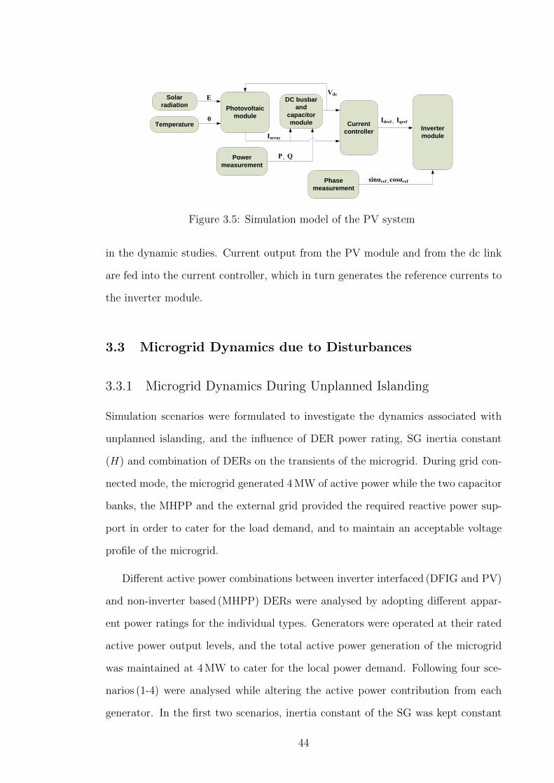
Solar radiation

Temperature

Photovoltaic module

DC busbar and

capacitor module Current

controller

Power measurement

Phase measurement

Inverter module

Idref , Iqref

P , Q

Vdc

Iarray

sinαref , cosαref

E

θ

Figure 3.5: Simulation model of the PV system

in the dynamic studies. Current output from the PV module and from the dc link

are fed into the current controller, which in turn generates the reference currents to

the inverter module.

3.3 Microgrid Dynamics due to Disturbances

3.3.1 Microgrid Dynamics During Unplanned Islanding

Simulation scenarios were formulated to investigate the dynamics associated with

unplanned islanding, and the influence of DER power rating, SG inertia constant

(H) and combination of DERs on the transients of the microgrid. During grid con-

nected mode, the microgrid generated 4 MW of active power while the two capacitor

banks, the MHPP and the external grid provided the required reactive power sup-

port in order to cater for the load demand, and to maintain an acceptable voltage

profile of the microgrid.

Different active power combinations between inverter interfaced (DFIG and PV)

and non-inverter based (MHPP) DERs were analysed by adopting different appar-

ent power ratings for the individual types. Generators were operated at their rated

active power output levels, and the total active power generation of the microgrid

was maintained at 4 MW to cater for the local power demand. Following four sce-

narios (1-4) were analysed while altering the active power contribution from each

generator. In the first two scenarios, inertia constant of the SG was kept constant

44

for different generator ratings according to (3.1), where the stored kinetic energy

varied with the SG rating. In the last two scenarios, the SG inertia constant was

varied with the machine capacity in order to maintain the same stored kinetic energy

in accordance with (3.1).

H =1/2Jω2

S(3.1)

where, S is the generator rated apparent power, J is the machine inertia, and ω is

the machine speed.

Both the DFIG and PV system were operated in unity power factor mode. Dur-

ing grid connected mode, frequency reference was taken from the external grid, while

in islanded mode, the microgrid frequency was controlled by the MHPP. The MHPP

operated in voltage control mode and 100% SG corresponds to the scenario where

the MHPP operated at rated power output (4 MW). The DFIG and PV system were

operated at unity power factor.

Scenario 1:

0 50 100 15049.0

49.5

50.0

50.5

51.0

51.5

52.0

Time (s)

Freq

uenc

y (H

z)

SG 100%SG 75%SG 50%SG 25%

Figure 3.6: Power frequency variations of the microgrid due to unplanned islandingwith different combinations of DFIG and MHPP

In this scenario, a MHPP and a DFIG were connected to Bus bars 646 and 680

45

respectively to supply the active power demand of the microgrid. Inertia constant

of the SGs were kept constant and the microgrid system was isolated from the bulk

supply point at t = 5 s to simulate a sudden unplanned islanding.

Scenario 2:

In order to observe the impact of DER type, the DFIG connected to the microgrid

in Scenario 1 was replaced with a PV system having the same power rating. The

microgrid system was isolated from the bulk supply point at t = 5 s to simulate a

sudden unplanned islanding.

0 50 100 15048.5

49.0

49.5

50.0

50.5

51.0

51.5

52.0

Time (s)

Freq

uenc

y (H

z)

SG 100%SG 75%SG 50%SG 25%

Figure 3.7: Power frequency variations of the microgrid due to unplanned islandingwith different combinations of PV and MHPP

Scenario 3:

In this scenario, a MHPP (with varying inertia constant) and a DFIG were connected

to Bus bars 646 and 680 respectively to supply the active power demand of the

microgrid. Ratings of the DERs were changed such that the total stored energy of

the SG was maintained at a constant level. The microgrid system was isolated from

the bulk supply point at t = 5 s to simulate a sudden unplanned islanding.

46

0 50 100 15049.0

49.5

50.0

50.5

51.0

51.5

Time (s)

Freq

uenc

y (H

z)

SG 100%SG 75%SG 50%SG 25%

Figure 3.8: Power frequency variations of the microgrid due to unplanned islandingwith different combinations of DFIG and MHPP (for different H values)

Scenario 4:

In order to observe the impact of DER type, the DFIG connected to the microgrid

in Scenario 3 was replaced with a PV system having the same power rating. The

microgrid system was isolated from the bulk supply point at t = 5 s to simulate a

sudden unplanned islanding.

0 50 100 15049.0

49.5

50.0

50.5

51.0

51.5

Time (s)

Freq

uenc

y (H

z)

SG 100%SG 75%SG 50%SG 25%

Figure 3.9: Power frequency variations of the microgrid due to unplanned islandingwith different combinations of PV and MHPP (for different H values)

Both Fig. 3.6 and Fig. 3.7 related to Scenario 1 and 2 exhibit similar responses to

unplanned islanding of the microgrid, irrespective of the combination of the DERs.

47

It can be observed that the magnitude of the maximum deviation of microgrid

frequency increases as the non-inverter interfaced DER (MHPP) capacity is reduced.

This occurs as the stored kinetic energy is increased in the SG with the reduction

of machine rating for the same inertia constant.

In Scenario 3 and 4, the SG inertia was varied according to the machine capacity

in order to maintain a constant stored energy. Both Fig. 3.8 and Fig. 3.9 exhibit

similar responses in relation to unplanned islanding of the microgrid, irrespective of

the combinations of the DERs. Before islanding, the surplus active power generated

in the microgrid was exported to the external grid. After islanding, active power

generation from the MHPP was reduced by the turbine governor controller in order

to maintain the microgrid frequency at 50 Hz. In this scenario, it can be observed

that the higher contribution of active power from the inverter interfaced DERs leads

to reduced oscillations in the power frequency of the islanded microgrid. According

to (3.1), this is due to the inertia constant of the SG which was increased with the

reduction of machine rating, as both DFIG and PV were operated in constant power

factor mode and did not contribute to the total inertia of the system. In all four

scenarios, the power frequency oscillations due to the unplanned islanding of the

microgrid were mainly determined by the inertial characteristics of the SG of the

MHPP.

The maximum rate of change of frequency (ROCOF) of the microgrid for all

four scenarios are summarised in Table 3.2 and Table 3.3. Due to lack of available

inertial response from DFIG and PV systems, inertial response was provided only by

the MHPP in the microgrid. Hence, effective angular acceleration of the SG would

increase, resulting in an increase in the maximum ROCOF. This can be clearly

observed from Table 3.2 and Table 3.3, where the maximum ROCOF occurred with

25% active power contribution from the MHPP in the microgrid. Therefore, design

of islanding protection schemes for microgrids consisting of both inverter and non-

inverter based DERs need to be carried out giving special attention to the proportion

of each type of DER.

48

Table 3.2: Maximum ROCOF for Scenario 1 and Scenario 2

Active power contribution Maximum ROCOF (Hz/s)from the MHPP DFIG and MHPP PV and MHPP

25% 16.71 12.4850% 13.54 7.7175% 5.38 3.36100% 1.00 0.96

Table 3.3: Maximum ROCOF for Scenario 3 and Scenario 4

Active power contribution Maximum ROCOF (Hz/s)from the MHPP DFIG and MHPP PV and MHPP

25% 16.64 11.8950% 13.54 7.7175% 6.11 3.69100% 1.44 1.41

Table 3.4 presents the minimum voltage at the grid connection point as a per-

centage of steady state voltage during unplanned islanding of the microgrid corre-

sponding to Scenario 3. It can be observed that with the increased penetration of

MHPP, voltage sag level has improved due to the reactive power support provided

by the SG.

Table 3.4: Minimum voltage magnitude as a percentage of the steady state voltageduring islanding for Scenario 3

Active power contribution Minimum voltage/ Steady state voltage (%)from the MHPP

25% 91.0550% 92.6075% 92.90100% 93.20

3.3.2 Dynamic Characteristics in Grid Connected and Islanded Modes

due to Large Disturbances

In this section, four different scenarios were analysed in order to investigate dy-

namic characteristics due to large disturbances of a microgrid in grid connected and

49

islanded modes. In the first scenario, impact of the type of DER on fault recovery of

a grid connected microgrid was analysed. In the second scenario, a comparison was

carried out on post fault behaviour in grid connected and islanded modes. Effects

of the type of the DER control mode on the fault recovery was analysed in the third

scenario. In the fourth scenario, the microgrid was subjected to a sudden increase

in load and the post disturbance behaviour was analysed for grid connected and

islanded modes.

Scenario 1:

In this scenario, the post fault behaviour of individual DERs in a grid connected

microgrid and the dynamic response of the external grid were analysed. During

the steady state, the total active power demand of the microgrid was met by an

individual DER. The MHPP was operated at the terminal voltage control mode

and 100% MHPP corresponds to the scenario where the MHPP generated the entire

4 MW of active power. Both DFIG and the PV system were operated at unity power

factor. A three-phase short-circuit fault was applied to Bus bar 634 at t = 120 s and

cleared after 150 ms.

118 119 120 121 122 123 124 125 1262.0

2.5

3.0

3.5

4.0

4.5

5.0

5.5

6.0

6.5

Time (s)

DE

R A

ctiv

e Po

wer

(M

W)

100% MHPP100% DFIG100% PV

Figure 3.10: Active power output from the DERs in grid connected mode

It can be observed from Fig. 3.10 and Fig. 3.11 that only the MHPP contributes to

the post fault oscillations of the microgrid system that arises as a result of its inertia,

50

118 119 120 121 122 123 124 125 126−5

0

5

10

15

Time (S)

Ext

erna

l grid

Act

ive

Pow

er (

MW

)

100% MHPP100% DFIG100% PV

Figure 3.11: Active power supply from the external grid in grid connected mode

whereas both DFIG and the PV system respond to the fault fast and stabilises the

DER output through fast PQ controllers.

Scenario 2:

In order to analyse the post fault behaviour of the microgrid, the same three-phase

short-circuit fault was applied to Bus bar 634 at t = 120 s and cleared after 150 ms

during grid connected and islanded modes. In this scenario, the total active power

for the microgrid was supplied by an MHPP and a PV system. The MHPP was

operated at the terminal voltage control mode and 100% SG corresponds to the

scenario where the MHPP operated at rated power output (i.e. 4 MW), while the

PV system was operated at unity power factor.

Compared to the islanded mode, post fault frequency of the microgrid in grid

connected mode recovers quickly resulting from the support from the external grid

(refer Fig. 3.12 and Fig. 3.13). According to Fig. 3.12, less power contribution from

the MHPP of the microgrid in grid connected mode is favourable for damping the

post fault oscillations. As expected, Fig. 3.13 and Fig. 3.14 demonstrate that an

increase in the power contribution from the PV system negatively affects damping

of post fault transients of the hybrid microgrid in islanded mode.

51

--

1£: 1\ -

JJ (\ A r. J v v ~

118 120 122 124 126 128 13049.9

50

50.1

Time (s)

Freq

uenc

y (H

z)

SG 100%SG 75%SG 50%SG 25%

Figure 3.12: Microgrid frequency variations due to a three-phase short-circuit faultin grid connected mode

120 130 140 150 160 170 180 190 20048

49

50

51

52

53

54

Time (s)

Freq

uenc

y (H

z)

SG 100%SG 75%SG 50%SG 25%

Figure 3.13: Microgrid frequency variations due to a three-phase short-circuit faultin islanded mode

Scenario 3:

Similar to the previous scenario, a three-phase short-circuit fault was applied to Bus

bar 634 at t = 120 s and cleared after 150 ms during grid connected mode. In this

scenario, the total active power for the microgrid was supplied by the combination of

the MHPP with both DFIG and PV systems separately. The MHPP was operated

at the terminal voltage control mode and 100% MHPP corresponds to the scenario

where the MHPP generated the entire 4 MW of active power. Both DFIG and the

52

118 120 122 124 126 128 1300

0.2

0.4

0.6

0.8

1

1.2

1.4

Time (s)

Vol

tage

(pu

)

SG 100% SG 75% SG 50% SG 25%

Figure 3.14: Voltage variations at Bus bar 652 due to the three-phase short-circuitfault in islanded mode

118 120 122 124 126 128 130−5

0

5

10

15

20

25

Time (s)

Rea

ctiv

e P

ower

(M

VA

r)

100% DFIG, p.f=1.0100% PV, p.f=1.0100% MHPP100% PV, p.f=0.93100% DFIG, p.f=0.89

Figure 3.15: Reactive power supply from the external grid for DERs operating atdifferent power factors

PV systems were operated at different power factors.

Fig. 3.15 illustrates the reactive power variations of the external grid while Fig.

3.16 illustrates the corresponding voltage variations at the microgrid PCC. A positive

value indicates the reactive power flow from external grid to the microgrid (power

import) and vice versa. A microgrid comprising only a DFIG which is operating at

unity power factor has the highest reactive power demand during the fault due to the

activation of crowbar protection. Least reactive power demand is from the MHPP,

53

-------------- l~~-~k-_9~---~--- -~-- ~-~--- -~--- -~-- -~--- -~--- -~---~--- -~--- -~--- -~-- -~---_,_--

-·-· -·-·-' -·-·-·--·-··-' -·-·-' -·-·-·-' -·-~------- ~~~------~~-~ :~-~-~~ ~~-~--~~ ~~--~~~-~~-~--~·~ :~--~~ ~·:_-~~-~ ~~~-~-----------------------------------------

118 119 120 121 122 123 124 125 1260.92

0.94

0.96

0.98

1.00

1.02

Time (s)

Vol

tage

at t

he P

CC

(pu

)

Figure 3.16: Voltages at the microgrid PCC for DERs operating at different powerfactors

which provides dynamic reactive power support during the fault. However, when the

DFIG and the PV system operate below unity power factor, the microgrid is able

to export reactive power to the external grid during the steady state. Furthermore,

post fault oscillations can only be seen when the microgrid comprises of a MHPP

which has a SG directly coupled to the network. In the absence of inertial response,

the DFIG and the PV system do not contribute to the post fault oscillations.

Scenario 4:

In this scenario, the microgrid was subjected to a 30% increase in both active

and reactive power demand by the load at Bus bar 652 during grid connected

and islanded modes. The total active power for the microgrid was supplied by

an MHPP (2.5 MVA) and DFIG system (2.5 MVA). The MHPP was operated in the

terminal voltage control mode and the DFIG system was operated in constant power

factor mode with a 0.89 lagging power factor.

During the grid connected mode, increase in load demand was catered by the

external grid. However, in the islanded mode, additional active and reactive power

demand from the load was provided by the MHPP as the DFIG was operating

in power factor control mode, dispatching predefined power levels as illustrated

54

120 130 140 150 160 170 180 190 2001.85

1.90

1.95

2.00

2.05

2.10

Time (s)

Act

ive

Pow

er (

MW

)

MHPP (grid tied mode)DFIG (grid tied mode)MHPP (islanded mode)DFIG (islanded mode)

Figure 3.17: Active power output of the MHPP and the DFIG due to a load increasein grid connected and islanded modes

118 120 122 124 126 128 130−0.2

0.0

0.2

0.4

0.6

0.8

1.0

1.2

Time (s)

Rea

ctiv

e P

ower

(M

VA

r)

MHPP (grid tied mode) DFIG (both modes) MHPP (islanded mode)

Figure 3.18: Reactive power output of the MHPP and the DFIG due to a loadincrease in grid connected and islanded modes

in Fig. 3.17 and Fig. 3.18. As expected, Fig. 3.19 and Fig. 3.20 illustrate that the

particular load increase has a negligible impact on the microgrid frequency and

voltage during grid connected mode.

55

120 140 160 180 200 220 24049.2

49.4

49.6

49.8

50.0

50.2

50.4

50.6

Time(s)

Freq

uenc

y (H

z)

Grid connected modeIslanded mode

Figure 3.19: Variations of the microgrid frequency due to a load increase in gridconnected and islanded modes

120 130 140 150 160 170 180 190 2000.98

0.99

1.00

Time (s)

Vol

tage

at t

he P

CC

(pu

)

Grid connected modeIslanded mode

Figure 3.20: Variations of the microgrid PCC voltage due to a load increase in gridconnected and islanded modes

3.4 Influence of External Grid Characteristics on the Grid

Connected Microgrid

3.4.1 Effect of External Grid Short-Circuit Capacity on Microgrid

Voltage

Impact of the short circuit capacity (SCC) of the external grid on the microgrid

was analysed by applying a three-phase short circuit fault to Bus bar 634 at t = 1s

for 150 ms. Active power demand of the microgrid was catered for by an MHPP

56

-

connected at Bus bar 646 and a DFIG at Bus bar 680 each having a capacity

of 2.5 MVA. Similarly, DFIG was replaced with a PV system, and the same fault

was applied to the microgrid. The magnitude of the maximum voltage sag at the

microgrid PCC for different SCC levels of the external grid are illustrated in Fig. 3.21.

200 400 600 800 1000 1200 1400 1600 1800 20000.06

0.08

0.10

0.12

0.14

0.16

0.06

0.08

0.10

0.12

SCC of the external grid (MVA)

Max

imum

vol

tage

dip

at t

he P

CC

(pu

)

MHPP and DFIGMHPP and PV

Figure 3.21: Variation of the maximum voltage dip at the PCC with the externalgrid SCC

As expected, the external grid with higher SCC levels provides better voltage

support to the grid connected microgrid. The microgrid with DFIG and MHPP

demonstrates a slightly larger voltage dip compared to the combination of PV and

MHPP as illustrated in Fig. 3.21. During the fault, voltage drop in the DFIG stator

windings produces sudden changes in the machine stator flux resulting a rapid in-

crease in the stator current. Due to the magnetic coupling between the stator and

the rotor, a high current will flow in the rotor and the converter. In order to protect

from high currents, crowbar resistors are used to bypass the converters. Activation

of these crowbar resistors converts the DFIG into a squirrel cage induction gener-

ator which consumes increased reactive power during voltage dips. Consequently,

high reactive power absorption results in larger voltage drop within the microgrid.

However, PV systems do not have such reactive power requirement: hence provide

better performance during voltage dips.

57

3.4.2 Effect of External Grid Inertia on Microgrid

Similar to the previous scenario, the same fault was applied in the microgrid and the

maximum ROCOF was observed for different external grid inertia levels. According

to Table 3.5, external grid inertia does not have a significant impact on the maximum

ROCOF for a particular combination of DERs. However, the microgrid with DFIG

and MHPP has indicated higher ROCOF values compared to microgrids with PV

and MHPP. As per Section 3.4.1, this is due to the larger power variation in the

DFIG compared to PV system during the fault.

Table 3.5: Maximum ROCOF for different external grid inertia constants

External grid inertia constant (s) Maximum ROCOF (Hz/s)With DFIG & MHPP With PV & MHPP

4 0.02486 0.008436 0.02490 0.0086510 0.02496 0.0090114 0.02500 0.0092818 0.02503 0.00947

3.5 Summary

In this chapter, preliminary investigations of the dynamic characteristics of mi-

crogrids under different operating conditions were carried out using time domain

simulations. Simulations were undertaken using DIgSILENT PowerFactory by de-

veloping a microgrid network comprising a PV system, a DFIG and an MHPP as

DERs and local loads. Dynamic impact of a range of aspects such as different

inherent characteristics of DERs, different power dispatch levels, generator capaci-

ties, and external grid characteristics on microgrid operation were analysed under

different scenarios.

It was clearly evident that the DERs with a directly coupled rotor to the network

have a significant influence on the post fault oscillations in the microgrid as the

inertial response of inverter interfaced DER is either unavailable (e.g. PV system) or

decoupled from the network (e.g. DFIG). Microgrids with smaller system rotational

58

inertia have a larger frequency deviation for a given mismatch between load and

the power generation. However, depending on the speed, accuracy and artificial

damping provided by the controllers, the inverter interfaced DERs would also have

a substantial impact on the microgrid stability. The fast controllers will allow the

inverter interfaced DERs to respond to disturbances quickly and reach the steady

state after a fault clearance.

When different DER types are operating simultaneously in a microgrid, special

care must be taken in designing the protection schemes such as microgrid islanding

detection. Special attention is also required when a microgrid is transferring from

grid connected mode to islanded mode, as the operation of mixed DER types exhibit

different responses with and without the external grid. In addition, dynamic reactive

power compensation and emulated frequency response schemes must be implemented

in microgrids to preserve voltage and frequency stability when operating in islanded

mode.

Microgrids operating in parallel with the external grid have a higher power supply

reliability. It was highlighted that the external grid SCC plays an important role in

maintaining an acceptable microgrid voltage profile. The study has shown that the

dynamic characteristics of the microgrid are significantly influenced by the individual

characteristics of DERs and their control systems. Furthermore, studies have also

shown that different power dispatch levels, generator MVA capacities, and external

grid characteristics also influence the dynamic behaviour of the microgrid, thus these

factors should be considered when planning microgrids, and in particular designing

protection systems for the microgrid.

In the future, when microgrids become more commonplace with higher pene-

tration of DERs, the stability and security of the utility grid will be influenced

significantly. Thus, microgrids need to be designed properly to take care of their

dynamic impact on the utility grid such that overall stability and reliability of the

whole system is significantly improved.

59

Chapter 4

Dynamic Equivalent of a Grid

Connected Microgrid -

Methodology and Modelling

4.1 Introduction

In many engineering applications, complex mathematical models can be derived to

represent the dynamic behaviour of individual components and systems. Although

a complicated higher order mathematical model will generally more accurately rep-

resent system dynamics, sometimes it is often desirable to have a simplified reduced

order model which will retain the important features of the system, but limit re-

quirements of computational and data storage capabilities.

In traditional power system analysis, dynamics of distribution networks were

not required to be considered in stability studies as networks were generally passive.

However, with the increasing penetration of DERs and grid connected microgrids,

distribution networks have begun to feature active characteristics with bidirectional

power flows. Hence, such systems can no longer be represented merely by using

static load models. It is impractical for utilities to represent individual and com-

bined DERs as detailed models in power system simulations, and this has led to

60

a need for new and accurate simplified models of grid connected microgrids. Such

simplified models of microgrids will be useful to electric utilities in performing dy-

namic studies by representing grid connected microgrids as simplified generators or

loads depending on the power export and import status at the microgrid PCC.

This chapter is focused on a model equivalencing methodology applicable to grid

connected microgrids comprising both inverter and non-inverter interfaced DERs.

The objective is to present a novel application of modal analysis for representing grid

connected hybrid microgrids as reduced order single entities suitable for power sys-

tem studies by preserving the important dynamics. The model reduction approach

is presented in this chapter outlining the dynamic models of individual dynamic

components. Validation of the model equivalencing approach is carried out using

various case studies in Chapter 5.

A discussion on the selection of a suitable dynamic model equivalencing method-

ology for grid connected microgrids is presented in Section 4.2. Section 4.3 covers the

theory behind the model equivalencing methodology selected for the work presented

in this thesis. Section 4.4 presents modelling details of an inverter interfaced DER,

a conventional DER, loads and the network of a grid connected microgrid suitable

to be used in model equivalencing methodology, followed by the chapter summary

in Section 4.5.

4.2 Selection of the Dynamic Model Equivalencing Method-

ology for Grid Connected Microgrids

As explained in Section 4.1, model equivalencing or reduction is to replace a given

complex mathematical model of a system with a less complex model which would

still capture all the important dynamics associated with the original system. Model

equivalencing involves a trade off between model order and the degree to which the

characteristics of the original system are reflected in the reduced model.

61

For stability analysis, the common practice is to separate the power system into

a study area of interest and external areas. In general, the study area is represented

in a detailed manner while external areas are represented by dynamic equivalents

[45,46]. These equivalent models will approximate the effects of the external systems

on the study system, as parts of the system electrically far away from a disturbance

will have little effect on the study system dynamics, hence, it is unnecessary to

model them with greater accuracy.

As empahsised in Chapter 2, coherency based methods which identify coherent

groups of generators governed by generator rotor behaviour following a disturbance,

cannot be applied to modern inverter interfaced DERs due to decoupling of rotor

dynamics from the network (e.g. DFIGs and microturbines) or due to the absence of

such rotor dynamics (e.g. PV and battery storage systems). Out of the three main

methods stated in Chapter 2, only system identification methods use measured data

to select model parameters of the dynamic equivalent model. The model parame-

ters need to be adjusted with proper training algorithms using a large amount of

data sets, which is time consuming. Furthermore, these methods lack strong math-

ematical background compared to modal methods, and the estimated parameters

do not properly interpret the physical relevance to the dynamic equivalent of power

systems.

Generally, in modal methods, reduction of the linearised system is carried out by

removing the eigenvalues located furthest from the origin, and retaining the eigen-

values with small negative real parts and the less damped eigenvalues. The relevant

variables with respect to that principle are kept and the remaining variables are

expressed in terms of the dominant variables. Thus, overall dynamic characteris-

tics of the reduced system will be similar to the original system. Unlike system

identification methods which depend on parameter estimation, traditional model

equivalencing methodologies are firmly based on mathematical concepts and have

significant physical relevance to the system dynamics. However, care must be taken

in applying modal methods for systems with inverter interfaced DERs, as their state

62

variables are not well known as in the case of conventional SGs.

As mentioned in Chapter 2, the basic modal method has not been applied to grid

connected hybrid microgrids as a means for deriving dynamic equivalent models.

Thus, this chapter takes an approach in investigating the applicability of modal

analysis as a tool for dynamic model equivalencing of grid connected microgrids

containing inverter and non-inverter interfaced DERs.

4.3 Dynamic Model Equivalencing Methodology

The dynamic model reduction process covered in this section is illustrated in Fig. 4.1.

As explained in Chapter 2, while appropriate for conventional systems based on SGs,

selective modal analysis [50, 51] was considered not suitable for hybrid microgrids.

This is due to the difficulty in determining the significant states of inverter-interfaced

DERs at the initial stages of the method without carrying out a full eigenvalue

analysis. From various modal methods available in the literature, the matrix trans-

formation technique in [46] was selected and adapted for this work, as it allowed

full eigenvalue analysis of the hybrid microgrid model. In this approach, an addi-

tional step is introduced to identify and group the dominant system modes which

are to be retained in the dynamic equivalent microgrid model. Furthermore, the

grid connected microgrid is represented in a similar way to any other grid connected

dynamic device suitable for power system stability studies. The steps (Blocks A, B,

C and D in Fig. 4.1) associated with the enhanced model equivalencing process are

described in the following subsections.

4.3.1 Linearised Microgrid Model

For the purpose of stability analysis of large power systems, microgrids connected

outside the study area of interest can be represented as linear systems [45, 46].

Influence of the control systems and inherent dynamic characteristics of DERs and

loads are captured by modelling these elements using ordinary differential equations,

63

Network data, generator and control

dataLoad flow

Calculation of eigenvalues and

eigenvectors

Identification of dominant modes

Rearrange coefficient matrices corresponding to

dominant modes

Construction of linearised microgrid

model

Initialisation of state space model

Obtain the reduced order model

A

B

D

C

Figure 4.1: Model reduction approach applied to grid connected microgrids basedon the enhanced modal method

which in turn used to develop the state space model of the microgrid. From the

study system point of view, a microgrid can be seen as a single generator or load in

a linearised state-space form as follows:

64

∆x = AMG∆x+BMG∆vpcc (4.1)

∆ypcc = CMG∆x+DMG∆vpcc (4.2)

[∆ypcc] =

∆ipcc

∆ωref

(4.3)

where, AMG (n × n), BMG (n × 1), CMG (m × n), and DMG (m × 1) are coefficient

matrices of the system.

Vector ∆x contains states of the dynamic devices in the microgrid while vec-

tor ∆vpcc represents the voltage at the microgrid PCC as an input to the system.

Current through the microgrid PCC, ∆ipcc , and speed deviation of the microgrid

reference d-q frame ∆ωref are taken as the microgrid outputs in the vector ∆ypcc.

Derivation of (4.1) and (4.2) are explained in detail using a microgrid model in Sec-

tion 4.4. A block diagram of a grid connected microgrid expressed by (4.1) and (4.2)

is illustrated in Fig. 4.2. Time domain solutions to the state space equation given in

(4.1) and (4.2) are obtained from the following equations:

x(t) = eAMGtx(t0) +

t∫t0

eAMG(t−τ)BMGvpcc(τ)dτ (4.4)

y(t) = CMGeAMGtx(t0) + CMG

t∫t0

eAMG(t−τ)BMGvpcc(τ)dτ +DMGvpcc(t)

4.3.2 Initialisation of the State-Space Model

Once the linearised microgrid model is constructed, the network, DERs and control

data are incorporated into the model, and the load flow results are used to initialise

the state-space model.

65

External system

NetworkDER 1 DER 2

PCCiPCCv

1DGv 2DGv

2DGi1DGi

ref

ref

Equivalent microgrid model

PCC

ref

Figure 4.2: Block diagram of the linearised state-space model of a grid connectedmicrogrid system comprising two DERs

4.3.3 Identification of Dominant Modes

Let the state space model of the system to be reduced be,

∆x = AMG∆x+BMG∆vpcc (4.5)

As the first step in identifying the dominant modes, a coordinate transformation

is carried out where it is possible to find a matrixP such thatAMG is transformed

into a diagonal form as follows:

∆x = P∆z (4.6)

MatrixP contains the eigen vectors of matrixAMG as the columns.

P =

ϕ11 ϕ12 · · · ϕ1n

ϕ21 ϕ22 · · · ϕ2n

......

...

ϕn1 ϕn1 · · · ϕnn

(4.7)

66

pi =

ϕ1i

ϕ2i

...

ϕni

(4.8)

P = [p1, p2, · · · · · · · · · pn] (4.9)

where, ϕi is the ith right eigenvector ofAMG corresponding to the ith eigenvalueλi.

Considering (4.5) - (4.9) [166],

∆z(t) = P−1AMGP∆z(t) + P−1BMG∆vpcc

= Λ∆z(t) + P−1BMG∆vpcc

= Λ∆z(t) +B′∆vpcc (4.10)

Λ =

λ1 0 · · · 0

0 λ2...

.... . .

...

0 · · · · · · λn

(4.11)

where, P−1AMGP = Λ, and Λ is a diagonal matrix with the eigenvalues of ma-

trixAMG. Hence, the original state-space model of the grid connected microgrid

represented in (4.5) is transformed into (4.10).

Modes corresponding to the eigenvalues with large negative real numbers are

considered as non-dominant modes which are assumed to reach the steady state

instantaneously following a step disturbance, compared to other modes. Hence,

non-dominant modes that have less impact on the study system when observed from

67

the microgrid PCC can be eliminated from the transformed system model (4.10).

It is important to retain the poorly damped oscillatory modes in the reduced order

equivalent model.

In this section, a new index is defined for identifying the dominant modes which

need to be retained in the reduced order equivalent microgrid model. The real part

of the eigenvalues (σi) normalised as a percentage of the real part of the eigenvalue

located furthest away from the origin (σmax) is used as an index for the selection of

dominant modes as expressed in (4.12).

σi−normalised =σiσmax

× 100 % (4.12)

4.3.4 Rearrangement of Matrices and Model Reduction

After identifying the dominant modes, let Λ be rearranged as in (4.13) such that γr and

γnr represent the modes to be retained in the reduced model and the modes to be

eliminated from the original model respectively. The relevant state variables corre-

sponding to the dominant modes are retained, and the remaining state variables are

expressed in terms of retained state variables. Rows of matrixB′in (4.10) also need

to be rearranged accordingly.

∆zr

∆znr

=

γr 0

0 γnr

∆zr

∆znr

+

B′r

B′nr

∆vpcc (4.13)

Reduced order system equation of (4.10) is given by,

∆zr = γr∆zr +B′

r∆vpcc (4.14)

where, zr- transformed states to be retained in the reduced model, znr- transformed

states assumed to reach the steady state instantly.

Contributions of state variables on the system modes are calculated using the

participation factors [163]. Participating factors indicate the relative participation

68

of the respective states in the corresponding modes. Participation factor of an lth

state variable on the mth mode is given by

plm = ϕlmφml (4.15)

where, ϕlm- lth element of the right eigenvector ϕm and φml- lth element of the left

eigenvector φm.

Next, (4.2) can be rearranged such that,

∆ypcc = Co/p∆xo/p +DMG∆vpcc (4.16)

where,xo/p- sub vector of ∆x comprising the original states contributing to the sys-

tem output, and Co/p is the sub matrix ofCMG comprising the columns correspond-

ing toxo/p.

In order to obtain the reduced order system output equation corresponding to

(4.2), transformation matrix P in (4.6) is rearranged as follows:

∆xo/p

∆xno/p

=

αr αnr

βr βrn

∆zr

∆znr

(4.17)

where,xno/p- sub vector of ∆x comprising the original states with no contribution to

the system output. The r rows corresponding to the states xo/p are placed in the

first r rows of matrix P while the first r columns are rearranged corresponding to

the retained r eigenvalues.

For a step input znr = 0, hence, using (4.13),

∆znr = −γ−1nr B

′

nr∆vpcc (4.18)

Using (4.17) and (4.18) in (4.16),

69

∆ypcc = Co/pαr∆zr − Co/pαnrγ−1nr B

′

nr∆vpcc +DMG∆vpcc

∆ypcc = C′∆zr +D

′∆vpcc (4.19)

where,C′=Co/pαr andD

′=DMG − Co/pαnrγ

−1nr B

′nr. Hence, the reduced order dy-

namic equivalent of the microgrid model corresponding to (4.1) and (4.2) is given

by (4.14) and (4.19).

This section described in detail all steps involved in modal reduction approach se-

lected to be applied to grid connected microgrids based on enhanced modal method.

This method is applied to a microgrid modelled as explained in the following section.

4.4 Modelling of the Microgrid for Model Equivalencing

This section presents the detailed modelling of an inverter interfaced DER, a non-

inverter interfaced DER, loads and the network of a grid connected microgrid suit-

able for implementation of the selected model equivalencing methodology. All dy-

namic devices in the microgrid are represented by state-space models.

4.4.1 Global Reference Frame

D

Q

1d

2d1q

2q

gbl

2

1

12

Figure 4.3: Global and local reference frames of the microgrid

In any microgrid system, it is necessary to define a global reference frame which

would allow all dynamic devices and other network components rotating on local

70

reference frames to be represented in a common reference frame. Transformation

from the local reference frames (di − qi) to the global reference frame (D − Q) is

carried out using (4.20).

[fQD] =

cos δi sin δi

− sin δi cos δi

[fqd]

[fQD] = [Ti][fqd] (4.20)

where, [fQD] - state variables in the global reference frame, [fqd] - state variables in

the local reference frame, and δi - angle between the d-axis of the global reference

frame and the d-axis of the local reference frame corresponding to the ith dynamic

device.

As illustrated in Fig. 4.2, when modelling the dynamic devices in a microgrid,

current injected to the microgrid from each device is taken as the output signal of

the device, and the respective terminal voltage of the device and the global reference

frame frequency deviation are taken as the input signals. As the model equivalencing

method is applied to linearised systems, (4.20) is linearised around an operating

point.

In order to connect a dynamic device into the microgrid, output signals (currents)

need to be expressed in the global reference frame as in (4.21) (it is assumed that

cos(∆δ) ' 1 and sin(∆δ) ' ∆δ).

∆IQ

∆ID

= [Tio]

∆Iq

∆Id

+

−Iqo sin δio + Ido cos δio

−Iqo cos δio − Ido sin δio

∆δ (4.21)

Similarly, the input voltage needs to be transformed from the global reference

frame to the respective local reference frame as follows:

71

∆Vq

∆Vd

= [Tio]−1

∆VQ

∆VD

+

−Vqo sin δio − Vdo cos δio

Vqo cos δio + Vdo sin δio

∆δ (4.22)

where, “” represents the steady state operating point around which the equations

are linearised.

4.4.2 Inverter Interfaced DER Model

For an inverter interfaced DER, it is be assumed that the output power of the dc

voltage source connected to the inverter is constant during the time frame of the

analysis. This will allow the dc side dynamics to be neglected in the converter model

and to represent inverter interfaced DER based on any power source. Thus, a generic

model is used to represent inverter interfaced DER units consisting of a constant

dc voltage source, a converter power circuit and converter controls. As illustrated

in Fig. 4.4, ac side of the converter is connected to the microgrid through a lumped

impedance having a reactance ofX and a resistance ofR. The ordinary differential

equations (ODE) describing the ac side of the converter can be expressed as follows:

Eabc = RIabc + LdIabcdt

+ Vabc (4.23)

Equation (4.23) is transformed into the local d-q reference frame defined at the

DER terminal, where d-axis is always coincident with the instantaneous voltage

vector, and the q-axis is in quadrature with it.

Eq = RIq + LdIqdt

+ ωinvLId (4.24)

Ed = Vd +RId + LdIddt− ωinvLIq

where, ωinv = dδinv/dt and δinv is the angle between the d-axis of the global reference

72

DCV

Converter

ACDC /

R Xabc

VabcE

aI

bI

cI

Figure 4.4: Inverter interfaced DER

frame and d-axis of the local reference frame of the corresponding inverter interfaced

DER. In order to decouple the Id and Iq components, a new variable is introduced

as follows [167]:

Vqnew = Eq − ωinvLId (4.25)

Vdnew = Ed − Vd + ωinvLIq

Equations (4.24) and (4.25) are linearised around an operating point and com-

bined to obtain the state-space format of the inverter as follows:

∆Xinv = Ainv∆Xinv +1

L∆Vqdnew (4.26)

where, ∆Xinv = [∆Iq2,∆Id2] and ∆Vqdnew = [∆Vqnew,∆Vdnew].

The mathematical model of the linearised phase locked loop (PLL) circuit illus-

trated in Fig. 4.5 is expressed by (4.27) [168].

ωinv = Kpll(Kp +Ki

s)(δref − δinv) (4.27)

∆ωinv = −KpllKpω∆ωinv −KpllKi∆δinv

where, Kpll is the gain of the input signal to the main PLL block, Kp and Ki are

73

A y y

_l_ v

~!YY

T v

ref

s1

sK

K ip

pllK

Figure 4.5: Linearised PLL circuit

the proportional and integral gains of the PI controller respectively.

In this chapter, the inverter interfaced DER is considered to be operated in

the constant power factor mode. The d-axis current component accounts for the

instantaneous active power, and the reference current for the d-axis current controller

loop is provided by the active power control loop as illustrated in Fig. 4.6. Linearised

equations describing the active power output of the DER are as follows:

Pout = V′

dI′

d + V′

q I′

q

∆Pout = Vdo∆I′

d + Ido∆V′

d + Vqo∆I′

q + Iqo∆V′

q (4.28)

Instantaneous power output of the DER is calculated using filtered instantaneous

voltage and current which are explained in (4.29).

∆I′

qd = − 1

Ti∆I

′

qd +1

Ti∆Iqd (4.29)

∆V′

qd = − 1

Tv∆V

′

qd +1

Tv∆Vqd

where, Ti and Tv are the time constants of the low pass filters of current and voltage

signals.

Linearised active power controller and d-axis current controller dynamics are

expressed in (4.30)-(4.33).

74

refP

s1

idKoutP

dii

pdK

drefI

ds1 die

pidK

iidKdnewV

L

qI’

dE

Vd'I

isT11

isT11

I

I

d

q

Figure 4.6: Active power controller and the d-axis current controller

∆idi = ∆Pref −∆Pout (4.30)

∆edi = ∆Idref −∆I′

d (4.31)

∆Idref = Kid∆idi +Kpd(∆Pref −∆Pout) (4.32)

∆Vdnew = Kiid∆edi +Kpid(∆Idref −∆I′

d) (4.33)

where, Kpd, Kpid and Kid, Kiid are the proportional and integral gains of the PI

controllers respectively.

Similarly, the reference for the q-axis current controller is generated using the

reactive power control loop as illustrated in Fig. 4.7. Corresponding linearised equa-

tions for the reactive power output of the DER, reactive power controller and the

q-axis controller can be described using (4.34) - (4.38).

Qout = V′

dI′

q − V′

q I′

d

∆Qout = Vdo∆I′

q + Iqo∆V′

d − Vqo∆I′

d − Ido∆V′

q (4.34)

75

refQ

s1

iqKoutQ

qii

pqK

qrefI

qI’s1 qie

piqK

iiqK qnewV

L

dI’

qEVq

I

I

q

d

isT11

isT11

Figure 4.7: Reactive power controller and the q-axis controller

∆iqi = ∆Qref −∆Qout (4.35)

∆eqi = ∆Iqref −∆I′

q (4.36)

∆Iqref = Kiq∆Iqi +Kpq(∆Qref −∆Qout) (4.37)

∆Vqnew = Kiiq∆eqi +Kpiq(∆Iqref −∆I′

q) (4.38)

where, Kpq, Kpiq and Kiq,Kiiq are the proportional and integral gains of the PI

controllers respectively.

Let the state variables and the disturbance inputs of the controllers be

∆Xcon = [∆V′q ,∆V

′

d ,∆I′q,∆I

′

d,∆iqi,∆idi,∆eqi,∆edi,∆ωinv] and

∆Uinv = [∆Qref ,∆Pref ] respectively. Then, (4.33) and (4.38) can be written in

terms of ∆Xcon and ∆Uinv.

∆Vqdnew = E1∆Xcon + E2∆Uinv (4.39)

Hence, state-space model of the converter (4.26) can be expressed in terms of

controller state variables as in (4.40).

76

∆Xinv = Ainv∆Xinv +1

L(E1∆Xcon + E2∆Uinv) (4.40)

Combining (4.27), (4.29)-(4.31), (4.35) and (4.36) will give the linearised state-

space model of the active and reactive power controllers of the inverter interfaced

DER.

∆Xcon = Acon∆Xcon +Bcon1∆Xinv +Bcon2∆Vqd +Bcon3∆Uinv (4.41)

∆yinv = Cinv∆Xinv +Dinv∆Vqd

Inverter interfaced DER in the local reference frame is established using (4.40)

and (4.41).

∆Xinv

∆Xcon

=

Ainv E1/L

Bcon1 Acon

∆Xinv

∆Xcon

+

0

Bcon2

∆Vqd (4.42)

+

E2/L

Bcon3

∆Uinv

Prior to connecting the inverter interfaced DER to the network, output sig-

nals (currents) are transferred to the global reference frame, and input signals (terminal

voltages) are transferred to the local reference frame. Substitution of (4.21) and

(4.22) in (4.42) describes the total inverter interfaced DER system as follows:

∆XIIDER = AIIDER∆XIIDER +BIIDER∆VQD−IIDER (4.43)

+ βIIDER∆UIIDER

∆IIIDER = CIIDER∆XIIDER +DIIDER∆VQD−IIDER

77

4.4.3 Non-Inverter Interfaced DER Model

In this section, a directly coupled SG is considered with a mini-hydro power plant

(MHPP) as the plant model comprising an exciter and a hydro turbine-governor

systems. The linearised ODEs of a salient-pole SG with damper windings on both

d-q axes and field winding on the d-axis together with the mechanical system are

expressed as follows [163]:

T′

do∆E′

q = ∆Efd −∆E′

q − (Xd −X′

d)∆Id

T′′

do∆E′′

q = −∆E′′

q + ∆E′

q − (X′

d −X′′

d )∆Id (4.44)

T′′

qo∆E′′

d = −∆E′′

d + (Xq −X′′

q )∆Iq

In per unit domain,

∆δ = ωb∆ωrpu

∆ωrpu =1

2H(∆Tm −∆Te) (4.45)

Te = E”q Iq + E”

dId − (X”d −X”

q )IdIq

Algebraic equations describing the voltage current relationship are as follows:

∆Vq = ∆E′′

q −R∆Iq −X′′

d∆Id

∆Vd = ∆E′′

d −R∆Id +X′′

q ∆Iq (4.46)

where, Vq and Vd are the axial components of the DER terminal voltage.

Fig. 4.8 illustrates the excitation model [163] which is described by the set of

equations in (4.47).

78

tVrefV

fdEr

r

TK1 a

a

TK1 ee sTK

1

f

f

sTsK1

1V

3V

aV

Figure 4.8: IEEE type-AC1A excitation system

∆V1 = − 1

Tr∆V1 +

Kr

Tr∆Vt

∆Va = −Ka

Ta∆Va −

Ka

Ta∆V3 −

1

Ta∆Vref +

Ka

Ta∆Vref (4.47)

∆V3 =Kf

TfTe∆Va −

1

Tf∆V3 −

KeKf

TeTf∆Efd

∆Efd =1

Te∆Va −

Ke

Te∆Efd

Fig. 4.9 illustrates a linear approximation of the turbine governor model [163]

and the corresponding ODEs are as follows:

∆X1 =1

Rp

∆ω

∆X2 =1

RT

∆X1 +1

RTTR∆X1 −

Rp

RTTR∆X2

∆X3 = − 1

TG∆X3 +

1

TG∆X2 (4.48)

∆X4 = ∆Tm

∆X4 = − 2

Tω∆X4 +

2

Tω∆X3 − 2∆X3

Equations (4.44) to (4.48) are combined to obtained the complete linearised

MHPP model as described in (4.49).

79

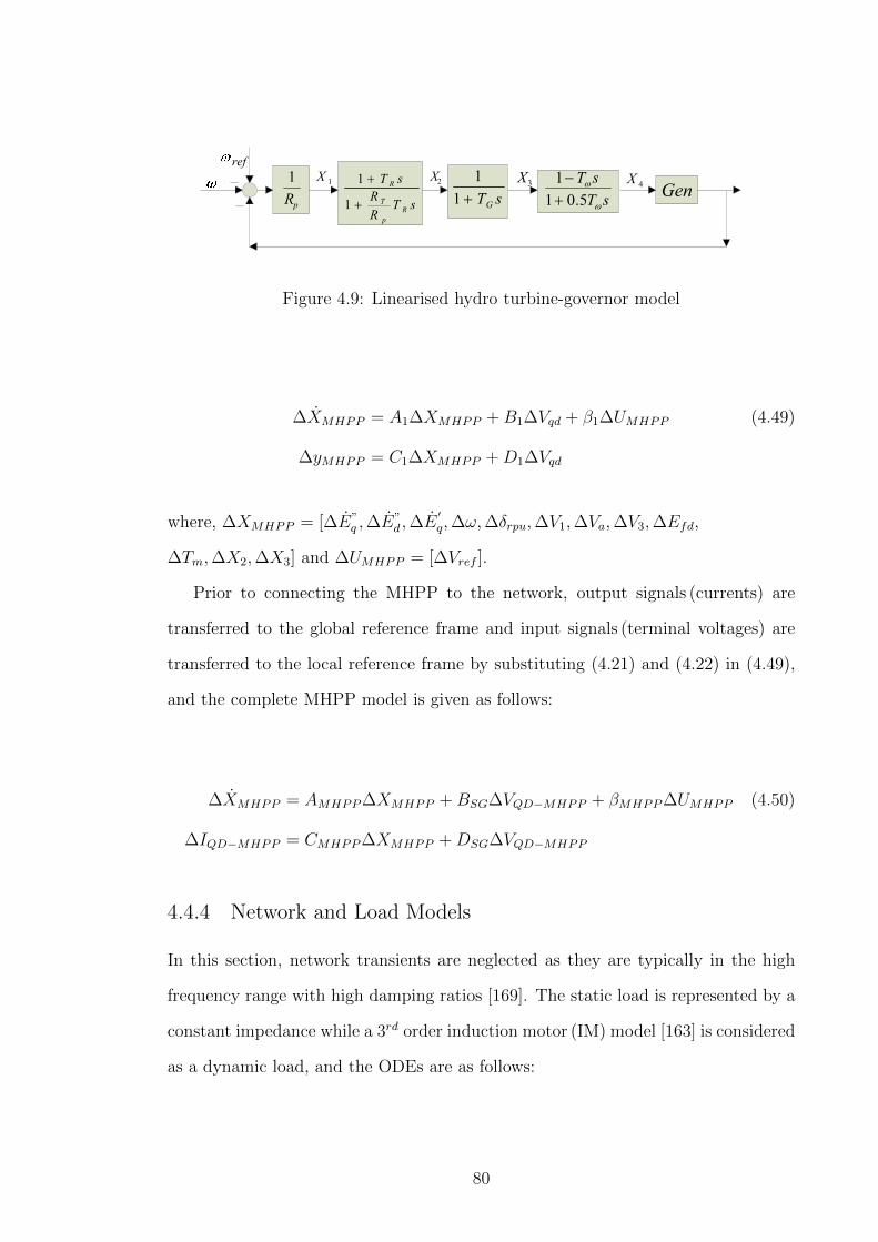
ref

GensT

RR

sT

Rp

T

R

1

1sTG1

1sTsT

5.011

pR1 1X 2X 3X 4X

Figure 4.9: Linearised hydro turbine-governor model

∆XMHPP = A1∆XMHPP +B1∆Vqd + β1∆UMHPP (4.49)

∆yMHPP = C1∆XMHPP +D1∆Vqd

where, ∆XMHPP = [∆E”q ,∆E

”d ,∆E

′q,∆ω,∆δrpu,∆V1,∆Va,∆V3,∆Efd,

∆Tm,∆X2,∆X3] and ∆UMHPP = [∆Vref ].

Prior to connecting the MHPP to the network, output signals (currents) are

transferred to the global reference frame and input signals (terminal voltages) are

transferred to the local reference frame by substituting (4.21) and (4.22) in (4.49),

and the complete MHPP model is given as follows:

∆XMHPP = AMHPP∆XMHPP +BSG∆VQD−MHPP + βMHPP∆UMHPP (4.50)

∆IQD−MHPP = CMHPP∆XMHPP +DSG∆VQD−MHPP

4.4.4 Network and Load Models

In this section, network transients are neglected as they are typically in the high

frequency range with high damping ratios [169]. The static load is represented by a

constant impedance while a 3rd order induction motor (IM) model [163] is considered

as a dynamic load, and the ODEs are as follows:

80

sR sX

sIsV 'E

Figure 4.10: Induction machine equivalent circuit

E′

q = −ωssE′

d −1

T ′(E

′

q − (Xs −X′

s)Ids)

E′

d = ωssE′

q −1

T ′(E

′

d + (Xs −X′

s)Iqs)

ωr =1

2H(Te − Tm) (4.51)

s =ωs − ωrωs

Te = E′

dIds + E′

qIqs

where, s is the slip of the IM.

∆XIM = AIM∆XIM +BIM∆VQD−IM + βIM∆UIM (4.52)

∆IQD−IM = CIM∆XIM +DIM∆VQD−IM

where, ∆XIM = [∆E′q,∆E

′

d,∆ωr] and ∆UIM = [∆Tm].

The relationship between network voltages and currents referred to the global

reference frame is described by the node admittance matrix in (4.53), including the

constant impedance loads.

∆IQD = Y∆VQD

81

∆IQ1

∆ID1

...

∆IQm

∆IDm

=

G11 B11 · · · G1m B1m

−B11 G11 · · · −B1m G1m

......

......

...... · · · Gmm Bmm

...... · · · −Bmm Gmm

∆VQ1

∆VD1

...

∆VQm

∆VDm

(4.53)

4.4.5 Overall Grid Connected Microgrid Model

Node matrix in (4.53) is rearranged as in (4.54).

∆Idyn

∆Istat

∆Ipcc

=

Yd−d Yd−s Yd−pcc

Ys−d Ys−s Ys−pcc

Ypcc−d Ypcc−s Ypcc−pcc

∆Vdyn

∆Vstat

∆Vpcc

(4.54)

where, Idyn- current injected into the network by the dynamic devices, Istat- current

injected to the network by the nodes without dynamic devices, and Ipcc- current

injected into the network through the microgrid PCC.

As the currents injected into the microgrid by the nodes without dynamic loads

are taken as zero, (4.54) can be further modified as in (4.55).

∆Idyn

∆Ipcc

=

Y11 Y12

Y21 Y22

∆Vdyn

∆Vpcc

(4.55)

An expression for the current injected into the network by all the dynamic de-

vices in the microgrid is derived by combining the outputs of the state-space models

as follows:

82

∆IDER1

∆IDER2

...

∆IIM1

∆IIM2

...

=

CDER1 0 · · · 0 0 · · ·

0 CDER2 · · · 0 0 · · ·

· · · · · · · · · · · · · · · · · ·

0 0 · · · CIM1 0 · · ·

0 0 · · · 0 CIM2 · · ·

· · · · · · · · · · · · · · · · · ·

∆XDER1

∆XDER2

...

∆XIM1

∆XIM2

...

+

DDER1 0 · · · 0 0 · · ·

0 DDER2 · · · 0 0 · · ·

· · · · · · · · · · · · · · · · · ·

0 0 · · · DIM1 0 · · ·

0 0 · · · 0 DIM2 · · ·

· · · · · · · · · · · · · · · · · ·

∆VDER1

∆VDER2

...

∆VIM1

∆VIM2

...

∆Idyn = Cdyn∆Xdyn +Ddyn∆Vdyn (4.56)

An expression for the generator terminal voltages is obtained from (4.55) and

(4.56) as follows:

Y11∆Vdyn + Y12∆Vpcc = Cdyn∆Xdyn +Ddyn∆Vdyn

∆Vdyn = (Y11 −Ddyn)−1Cdyn∆Xdyn − (Y11 −Ddyn)−1Y21∆Vpcc

(4.57)

Similar to (4.56), state-space forms of individual dynamic devices are combined

to obtain the overall system model.

83

∆XDER1

∆XDER2

...

∆XIM1

∆XIM2

...

=

ADER1 0 · · · 0 0 · · ·

0 ADER2 · · · 0 0 · · ·

· · · · · · · · · · · · · · · · · ·

0 0 · · · AIM1 0 · · ·

0 0 · · · 0 AIM2 · · ·

· · · · · · · · · · · · · · · · · ·

∆XSG

∆XDG2

...

∆XIM1

∆XIM2

...

+

BDER1 0 · · · 0 0 · · ·

0 BDER2 · · · 0 0 · · ·

· · · · · · · · · · · · · · · · · ·

0 0 · · · BIM1 0 · · ·

0 0 · · · 0 BIM2 · · ·

· · · · · · · · · · · · · · · · · ·

∆VDER1

∆VDER2

...

∆VIM1

∆VIM2

...

+

βDER1 0 · · · 0 0 · · ·

0 βDER2 · · · 0 0 · · ·

· · · · · · · · · · · · · · · · · ·

0 0 · · · βIM1 0 · · ·

0 0 · · · 0 βIM2 · · ·

· · · · · · · · · · · · · · · · · ·

∆UDER1

∆UDER2

...

∆UIM1

∆UIM2

...

∆Xdyn = Adyn∆Xdyn +Bdyn∆Vdyn + βdyn∆Udyn (4.58)

Substituting (4.57) into (4.58) yields:

∆Xdyn = Adyn∆Xdyn +Bdyn(Y11 −Ddyn)−1Cdyn∆Xdyn−

Bdyn(Y11 −Ddyn)−1Y21∆Vpcc + βdyn∆Udyn

∆Xdyn = M1∆Xdyn +M2∆Vpcc + βdyn∆Udyn (4.59)

84

where, M1 = [Adyn +Bdyn(Y11 −Ddyn)−1Cdyn] and M2 = [−Bdyn(Y11 −Ddyn)−1Y21].

From (4.55) an expression for the current through the microgrid PCC can be

obtained as follows:

∆Ipcc = Y21∆Vdyn + Y22∆Vpcc

∆Ipcc = Y21(Y11 −Ddyn)−1Cdyn∆Xdyn − Y21(Y11 −Ddyn)−1Y21∆Vpcc + Y22∆Vpcc

∆Ipcc = N1∆Xdyn +N2∆Vpcc (4.60)

∆ωref = R∆Xdyn (4.61)

where, N1 = [Y21(Y11−Ddyn)−1Cdyn] and N2 = [−Y21(Y11−Ddyn)−1Y21 +Y22]. ∆ωref

corresponding to the global reference frame in the microgrid is taken as an output

from the microgrid model.

Equations (4.59) and (4.60) describe the microgrid in the form of (4.1) and (4.2).

Thus, the node matrix is rearranged and combined with the equations of the dynamic

devices in the microgrid such that the grid connected microgrid could be represented

in a form analogous to the standard model of a dynamic device connected to the

external grid.

4.5 Summary

The main objective of this chapter was to present a novel approach in representing

grid connected microgrids as reduced order dynamic equivalents suitable for power

system studies.

It was identified that the basic modal method had not been previously applied

to grid connected microgrids comprising both inverter and non-inverter interfaced

DERs as a model equivalencing methodology. This chapter presented the formu-

lation behind the model equivalencing methodology based on modal method while

introducing a new index to identify the dominant modes of the system. Representa-

85

tion of a microgrid as a single dynamic device connected to the external system was

also introduced in this chapter, which can be employed to derive the dynamic equiv-

alent of a grid connected microgrid. Furthermore, detailed modelling of an inverter

interfaced DER with power controllers, non-inverter interfaced DER with governor

and excitation controllers, induction motor load and network were presented as a

base for the studies covered in the next chapter.

86

Chapter 5

Dynamic Equivalent of a Grid

Connected Microgrid - Model

Validation

5.1 Introduction

This chapter is focused on the application of the dynamic equivalent methodology

explained in Chapter 4.

Mathematical models are developed in this chapter for different grid connected

microgrids following the modelling procedures presented in Chapter 4. Validity of

the dynamic model equivalencing approach is examined under different microgrid

operating conditions. Furthermore, the dynamic model equivalencing is applied on

microgrids in a multi-microgrid environment in order to show the feasibility of the

methodology.

Section 5.2 presents several case studies carried out on a five-bus microgrid sys-

tem comprising two DERs and two types of loads under different system operating

conditions. Scalability of the proposed microgrid model equivalencing approach

is demonstrated in Section 5.3 with a larger microgrid model based on the IEEE-

13 node test feeder [162]. In Section 5.4, the dynamic equivalencing approach is

87

applied to a multi-microgrid system. Section 5.5 presents a discussion on the imple-

mentation of the proposed methodology in simulation platforms, performance of the

proposed approach, and other practical aspects. A chapter summary is presented in

Section 5.6.

5.2 Case Study 1 - Five Bus System

External grid

DER 1 DER 2Load 1 Load 2

PCCBus 1 Bus 2 Bus 3 Bus 4

IM

baseMG

baseMG

V

S

69 kV

13.8 kV

10 MVA

13.8 kV

4.16 kV

Figure 5.1: Single line diagram of the Microgrid System - 1

In this section, the dynamic equivalent model was derived for a five-bus microgrid

model comprising two DERs and two loads. Different operating conditions such as

power export mode, power import mode, and load variations were considered in

order to validate the equivalent model. Steady state operating conditions of the

microgrid system were obtained from a load flow analysis conducted on a non-linear

microgrid model developed in DIgSILENT PowerFactory. As explained in Chapter 4,

linearised model of the microgrid system was developed and a full eigenvalue analysis

was carried out in MATLAB. In the microgrid system, the local reference frame of

DER 1 was locked to the rotor of DER 1, and the global d-q reference frame was

defined at the terminal of DER 1 (Bus 1). At the DER 2, local d-axis was assumed

to be in the direction of the voltage vector at Bus 4.

88

5.2.1 Power Import from the External Grid

The single line diagram of the Microgrid System - 1 consisting of a 13.8 kV radial

distribution feeder connected to the external grid (fault level = 1200 MVA, X/R=10)

through a 69 kV/13.8 kV, 10 MVA transformer is illustrated in Fig. 5.1. The study

system comprises a 5 MVA MHPP (DER 1) operating at terminal voltage control

mode (Bus 1), a 1.5 MW, unity p.f. inverter interfaced DER (DER 2) operating at

constant power factor control mode (Bus 4), a static load of 4.2 MW/1.2 MVAr at

Bus 2, and an induction motor load of 1.42 MW, 0.85 p.f. connected through a

13.8 kV/4.16 kV, 2 MVA transformer (Bus 3). Details of the parameters of the SG,

IM and the network are presented in the Appendix A, while the steady state op-

erating conditions are presented in Table 5.1. It can be observed that the external

grid was supplying active and reactive power to cater for the local demand of the

microgrid.

Table 5.1: Steady state operating conditions of the microgrid components in powerimport mode

Microgrid component Steady state operating condition

DER 1 4.00 MW/1.23 MVArDER 2 1.50 MW/0.00 MVArLoad 1 4.20 MW/1.20 MVArLoad 2 1.40 MW/0.84 MVAr

External grid 0.13 MW/0.88 MVAr

In order to validate the linearised MATLAB model, the microgrid was modelled

in DIgSILENT PowerFactory, and the same small disturbance was applied to both

models. Fig. 5.2 illustrates the responses of the current and voltage of DER 2 of the

microgrid system obtained from the linearisd DIgSILENT PowerFactory model and

MATLAB model for a 2 % step decrease in the real power output of DER 2 (Pout) at

t = 5 s respectively. Comparison of the results in Fig. 5.2 (a) and Fig. 5.2 (b) from

the DIgSILENT and MATLAB models indicates similar behaviour of the observed

signals. The slight differences between the results from DIgSILENT PowerFactory

model and the MATLAB model are due to the differences in the method of im-

89

plementation and the time delays associated with the measurement and calculation

blocks.

As described in Section 4.4.3 of Chapter 4, the dominant modes to be retained

in the equivalent model were calculated using the new indexσi−normalised. Fig. 5.3

illustrates the indices corresponding to all eigenvalues. For this particular case

study, modes corresponding to eigenvalues with normalised real parts less than

10.0 %, including two low frequency oscillatory modes were selected as the dominant

modes. Eigenvalues and the dominant states corresponding to the modes retained

in the equivalent microgrid model are given in Table 5.2. Corresponding matrices

γr, B′r, C

′, and D

′in (4.14) and (4.19) were calculated in MATLAB according to

the description given in Section 4.3 of Chapter 4, which reduced the 29th order model

to an 18th order equivalent model.

Responses of the full order model and reduced order model of the microgrid

system for a 2 % step decrease in active power output Pout of DER 2 at t = 5 s are

shown in Fig. 5.4. It can be observed from the figures that responses obtained from

the full order model and reduced order equivalent model are in good agreement.

Table 5.2: Dominant modes for the power import mode

Mode Eigenvalue Dominant states

5 -110 Exciter of the SG (∆V1)6 -74.4 Exciter of the SG (∆Efd)7 -37.3 Turbine-governor control of the SG (∆X1)

8,9 -2.05±12.95i Rotor angle and speed deviation of the SG (∆ω,∆δrpu)10 -3.08 Turbine-governor control of the SG (∆X2)11 -0.61 Exciter of the SG (∆V3)12 -1.09 Turbine-governor control of the SG (∆Tm)19 -149.0 Inverter state on DER 2 (∆Iq2)20 -148.8 Inverter state on DER 2 (∆Id2)

21,22 -10.98±11.41i Induction motor load (∆E′q,∆ωIM)

23 -4.87 d-axis current controller of DER 2 (∆edi)24 -4.85 q-axis current controller of DER 2 (∆eqi)

25 -21.9 Induction motor load (∆E′

d)26 -26.0 Active power controller of DER 2 (∆idi)27 -25.0 Reactive power controller of DER 2 (∆iqi)30 -129 Exciter of the SG (∆Va)

90

0 5 10 15

0.98

0.99

1

I DE

R2 (

pu)

0 5 10 151.0010

1.0011

1.0012

VD

ER

2 (pu

)

0 5 10 15

0.9996

1.0000

Time (s)

ωD

ER

1 (pu

)

(a)

0 5 10 15

−0.002

0

∆ID

ER

2 (pu

)

0 5 10 15

−0.0001

0

∆VD

ER

2 (pu

)

0 5 10 15

−0.0004

0

Time (s)

∆ωD

ER

1 (pu

)

(b)

Figure 5.2: System responses from (a) DIgSILENT model and (b) the MATLABmodel due to a 2 % step decrease in Pout of DER 2

91

0 2 4 6 8 10 12 14 16 18 20 22 24 26 28 300

20

40

60

80

100

Mode

σ i−no

rmal

ised

%

Power import modePower export mode

10.0 %

Figure 5.3: Normalised real parts of the eigenvalues for power import and exportmodes of the Microgrid System - 1

0 5 10 150

2

4

x 10−3

(a)

∆Idp

cc (

pu)

0 5 10 15

0

2

4

6

x 10−4

(b)Time (s)

∆Iqp

cc (

pu)

Full model Reduced model

Figure 5.4: Deviations of the d-axis and q-axis currents through the microgrid PCCdue to a 2 % step decrease in Pout of DER 2 in power import mode

5.2.2 Power Export to the External Grid

In this scenario, total load of the microgrid and the DER 1 (MHPP) rating were

unchanged relative to the previous scenario (power import mode) in Section 5.2.1,

while the rating of DER 2 was altered to 5 MVA operating at unity p.f. The cor-

responding steady state operating conditions are presented in Table 5.3, where the

negative values indicate power import into the microgrid. It can be observed that

92

the additional active power generated in the microgrid was fed to the external grid

while reactive power was supplied by the external grid to cater the local demand of

the microgrid. Similar to the previous scenario, modes corresponding to eigenvalues

with normalised real parts less than 10.0 %, including two low frequency oscillatory

modes were selected as the dominant modes as illustrated in Fig. 5.3. Eigenvalues

and the dominant states corresponding to the retained modes are given in Table 5.4,

reducing the 29th order model to a 18th order model. It is to be noted that the

eigenvalues have changed due to the change in the operating mode of the microgrid.

Table 5.3: Steady state operating conditions of the microgrid components in powerexport mode

Microgrid component Steady state operating condition

DER 1 4.00 MW/1.11 MVArDER 2 5.00 MW/0.00 MVArLoad 1 4.20 MW/1.20 MVArLoad 2 1.40 MW/0.84 MVAr

External grid -3.30 MW/1.15 MVAr

Table 5.4: Dominant modes for power export modes

Power export mode

Mode Eigenvalue Dominant states5 -111 Exciter of the SG (∆V1)6 -72.9 Exciter of the SG (∆Efd)7 -37.3 Turbine-governor control of the SG (∆X1)

8,9 -2.26±12.63i Rotor angle and speed deviation of the SG (∆ω,∆δrpu)10 -2.97 Turbine-governor control of the SG (∆X2)11 -0.61 Exciter of the SG (∆V3)12 -1.09 Turbine-governor control of the SG (∆Tm)19 -149.0 Inverter state on DER 2 (∆Iq2)20 -148.8 Inverter state on DER 2 (∆Id2)

21,22 -3.38±5.95i Induction motor load (∆E′q,∆ωIM)

23 -25.1 Active power controller of DER 2 (∆idi)24 -25.0 Reactive power controller of DER 2 (∆iqi)

25 -6.76 Induction motor load (∆E′

d)26 -4.93 d-axis current controller (∆edi)27 -4.90 q-axis current controller (∆eqi)30 -129 Exciter of the SG (∆Va)

Responses of the full order model and reduced order equivalent model of the

93

0 5 10 15

−10

−5

0x 10

−3

(a)

∆Idp

cc (

pu)

0 5 10 15

−6

−4

−2

0x 10

−4

(b)Time (s)

∆Iqp

cc (

pu)


Figure 5.5: Deviations of the d-axis and q-axis currents through the microgrid PCCdue to a 2 % step decrease in Pout of DER 2 in power export mode

microgrid system for a 2 % step decrease in active power output Pout of DER 2 at

t = 5 s are shown in Fig. 5.5. It can be observed from the figures that the disturbance

responses of the retained states and microgrid currents obtained from the equivalent

model are in good agreement with those of the full model.

5.2.3 Variation of Loading Conditions

In order to study the system mode variation under different loading conditions, two

different loading conditions were considered: (i) light load conditions with 50 % of

nominal load, and (ii) heavy loading conditions with 110 % of nominal load. Fig. 5.6

illustrates the effects of the loading conditions on eigenvalues corresponding to the

dominant modes of the microgrid system for both power import and export modes.

It is to be noted that the dynamic equivalent of the microgrid system changes with

system loading conditions. In Fig. 5.6, it can be observed that for the particular

study system, load variation has an insignificant effect on non-oscillatory modes.

As expected, with over loading conditions, oscillatory modes tend to move towards

the unstable region. However, for this particular system, oscillatory modes varied

within a very small region. Therefore, as the control strategies and controller param-

94

eters of DER units remained unchanged during grid connected operation, operating

conditions with nominal load were considered for obtaining the equivalent model.

Fig. 5.7 illustrates the deviations of the d-axis and q-axis currents through the mi-

crogrid PCC due to a 50 % load decrease in power import mode, obtained from the

full model and the equivalent model of the Microgrid System - 1. It is to be noted

that the dynamic equivalent of the microgrid system changes with system loading

conditions.

−150 −100 −50 0−15

−10

−5

0

5

10

15

Real (1/s)(a)

Imag

inar

y (r

ad/s

)

−150 −100 −50 0−15

−10

−5

0

5

10

15

Real (1/s)(b)

Imag

inar

y (r

ad/s

)

100 % load 50 % load 110 % load

Figure 5.6: Dominant modes under different loading conditions for (a) power import,and (b) power export modes in Microgrid System - 1

0 5 10 15−0.05

0

0.05

(a)

∆Idp

cc (

pu)

0 5 10 150

10

20x 10

−4

(b)Time (s)

∆Iqp

cc (

pu)


Figure 5.7: Deviations of the d-axis and q-axis currents through the microgrid PCCdue to a 50 % load decrease in power import mode

95

5.2.4 Response to Short-Circuit Faults

0 5 10 15−0.02

0

0.02

0.04

(b)Time (s)

∆Iqp

cc (

pu)

0 5 10 15−0.05

0

0.05

(a)

∆Idp

cc (

pu)


Figure 5.8: Deviations of the d-axis and q-axis currents through the microgrid PCCdue to a distant fault in power import mode

0 5 10 15−0.10

0

0.10

(a)

∆Idp

cc (

pu)

0 5 10 15−0.05

0

0.05

0.10

(b)Time (s)

∆Iqp

cc (

pu)


Figure 5.9: Deviations of the d-axis and q-axis currents through the microgrid PCCdue to a distant fault in power export mode

In this section, the impact of a reflection of a distant three-phase short-circuit

fault in the external grid on the microgrid PCC was analysed. A fault was created

in the external grid at t = 5 s and cleared after 0.5 s. It can be observed from

Fig. 5.8 and Fig. 5.9 that the reduced order equivalent model of the microgrid has

96

~ "

r-------v!'vv~~ --~

A

fvvv' v

f-------Vrvv-~--~

sufficiently captured the dynamic characteristics of the full order model during both

power import and export modes.

5.3 Case Study 2 - IEEE-13 Node Distribution Network

Bus 650DER 1

Bus 680

DER 2

DER 4

DER 3IM

Bus 646 Bus 645 Bus 632

Bus 611 Bus 684

Bus 652

Bus 671 Bus 692

Bus 633

Bus 675

Bus 634

External grid

baseMG

baseMG

V

S

115 kV

4.16 kV

50 MVA

4.16 kV

0.69 kV

0.69 kV

Figure 5.10: Single line diagram of the microgrid system based on the IEEE-13 nodedistribution test feeder

In order to demonstrate the scalability of the proposed microgrid model equiv-

alencing approach, a large microgrid system was developed based on the IEEE-13

node distribution test feeder [162]. As illustrated in Fig. 5.10, necessary modifica-

tions were made to the IEEE-13 node distribution test feeder in order to obtain

a three-phase balanced microgrid system. The microgrid system was connected to

the external grid through a 115 kV/4.16 kV, 10 MVA transformer. Two inverter

interfaced DERs (each rated at 0.5 MVA) operating at power factor mode were con-

nected to Bus bar 646 and Bus bar 634. Two SG based DERs of 1.5 MVA and 5 MVA

with exciter and governor controls were connected to Bus bar 680 and Bus bar 675

respectively. In addition to a static load, an induction motor load of 1.42 MW, 0.85

p.f. was connected to Bus bar 692. Load and network data of the 13 node micro-

grid system are presented in Appendix A. The grid connected microgrid exported

active power to the external grid and imported reactive power to cater for the local

97

demand.

In the microgrid system, the local reference frames of DER 3 and DER 4 were

locked to the rotors, and the global d-q reference frame was defined at the terminal

of DER 4. In DER 1 and DER 2, local d-axes were assumed to be in the direction of

the voltage vectors at Bus bar 646 and Bus bar 634 respectively.

−6000 −5000 −4000 −3000 −2000 −1000 0−1.5

−1

−0.5

0

0.5

1

1.5x 104

Real (1/s)

Imag

inar

y (r

ad/s

)

Figure 5.11: Eigenvalues of the 13 node microgrid system

Fig. 5.11 illustrates the eigenvalues of the microgrid system. From the eigen-

value analysis, three oscillatory modes were identified and selected to be retained

in the reduced order equivalent model. The remainder of the dominant modes were

identified using the normalised real part of eigenvalues as described in Section 4.3.3.

For this particular microgrid system, modes corresponding to the eigenvalues with

normalised real parts less than 5.0 % were selected as the non-oscillatory dominant

modes. Using the model equivalencing approach described in Section 4.3, the 54th

full order model was reduced to a 35th order equivalent model, and the retained

modes are presented in Table 5.5.

The reduced order microgrid model was subjected to several disturbances in

order to find the suitability of the proposed approach. Fig. 5.12 illustrates the sys-

tem responses of the microgrid due to a 0.1 pu step decrease in the output active

power (Pout) of DER 1 and DER 2 at t = 5 s and t = 10 s respectively. Furthermore,

98

Table 5.5: Dominant modes of the 13 node microgrid system

Mode Eigenvalue σi−normalised% Mode Eigenvalue σi−normalised%

5 -92.35 1.85 37 -49.46 0.986 -94.04 1.88 38,39 -1.98±17.13i 0.047 -27.82 0.56 40 -16.11 0.328 -27.23 0.55 41,42 -1.91±10.27i 0.049 -3.83 0.07 43,44 -1.96±7.20i 0.0410 -2.89 0.05 45 -6.08 0.1219 -6.73 0.13 46 -3.75 0.0720 -4.83 0.09 47 -2.78 0.0521 -31.19 0.62 48 -2.01 0.0422 -31.09 0.62 49 -0.64 0.0134 -202.4 4.04 50 -1.12 0.0235 -105.5 2.11 51 -0.83 0.0136 -79.47 1.58 54 -129.4 2.58

2 4 6 8 10 12 14 16 18 20

−4

−2

0

x 10−4

(a)

∆Idp

cc (

pu)

0 2 4 6 8 10 12 14 16

−10

−5

0x 10

−5

(b)Time (s)

∆Iqp

cc (

pu)


Figure 5.12: Deviations of the d-axis and q-axis currents through the microgrid PCCdue to a decrease in Pout of DER 1 and DER 2

deviations of the d-axis and q-axis currents through the microgrid PCC, and the

responses of the rotor speed of DER 3 and DER 4 due to a 50 % increase in the load

at Bus bar 646 at t = 5 s are illustrated in Fig. 5.13 and Fig. 5.14 respectively.

In addition, a three-phase short-circuit fault was created within the external

grid at t = 5 s and cleared after 0.5 s. The corresponding deviations of the currents

through the microgrid PCC are presented in Fig. 5.15.

It can be observed from Fig. 5.12 to Fig. 5.15, that responses obtained from

99

0 5 10 15−1

0

1x 10−3

(a)

∆Idp

cc (

pu)

0 5 10 15

−3

−2

−1

0x 10

−4

(b)Time (s)

∆Iqp

cc (

pu)


Figure 5.13: Deviations of the d-axis and q-axis currents through the microgrid PCCdue to an increase in load at Bus bar 646

0 5 10 15

−2

−1

0

1x 10

−4

(a)

∆ω3 (

pu)

0 5 10 15

−1

0

1x 10−4

(b)Time (s)

∆ω4 (

pu)


Figure 5.14: Deviations of rotor speed of the DER 3 and DER 4 due to an increasein load at Bus bar 646

the full model and reduced order equivalent model are in close agreement. The

selected modes have retained the important dynamics of the microgrid model, which

confirms the suitability of the proposed dynamic model equivalencing approach in

representing grid connected large microgrids for power system studies.

100

0 5 10 15−0.03

−0.02

−0.01

0

(a)

∆Idp

cc (

pu)

0 5 10 15

−4

−2

0

x 10−3

(b)Time (s)

∆Iqp

cc (

pu)


Figure 5.15: Deviations of the d-axis and q-axis currents through the microgrid PCCdue to a fault in the external grid

5.4 Case Study 3 - Multi-Microgrid System

In order to validate the model equivalencing approach on grid connected microgrids,

a multi-microgrid system illustrated in Fig. 5.16 is considered in this section. The

system comprises of three separate microgrids and a 5 MVA, 0.8 p.f. SG connected

to the 69 kV network through three 10 MVA, 69 kV/13.8 kV transformers and a

7.5 MVA, 69 kV/13.8 kV transformer respectively. The 69 kV network is connected to

the external grid through a 50 MVA, 115 kV/69 kV transformer. Network parameters

and load flow data of the multi-microgrid system are presented in Table 5.6 and

Table 5.7 respectively. The mode of operation of the five bus system described in

Section 5.2.1 were included in MG 1 and MG 2, whereas MG 3 is in the mode of

operation of the five bus system considered in Section 5.2.2.

Table 5.6: Network parameters of the multi-microgrid system

R (Ω/km) 0.1X (Ω/km) 0.3

Bus 3-Bus 1 (km) 2Bus 1-Bus 5 (km) 2Bus 2-Bus 5 (km) 2Bus 4-Bus 2 (km) 2

101

SG

External grid

baseMGS

Bus 1 Bus 2

Bus 3 Bus 4

Bus 5

MG 3

MG 2MG 1

115 kV

69 kV13.8 kV

50 MVA

Figure 5.16: Single line diagram of the multi-microgrid system

Table 5.7: Calculated load flow data of the multi-microgrid system

P (MW) Q (MVAr)

MG 1 -0.13 -0.49MG 2 -0.13 -0.49MG 3 3.31 -0.66SG 4.00 0.06

External grid -7.02 1.81

In this case study, the dynamic equivalent model of each microgrid system was

derived separately and connected to the 69 kV network along with a reduced order

SG model. Use of dynamic equivalent models for microgrid systems resulted in

a reduction of total system states from 103 to 59. Fig. 5.17 illustrates the selected

eigenvalues of the full order system and the eigenvalues from the system with reduced

order models. It can be observed that the system including the equivalent microgrid

modes have preserved the dominant eigenvalues of the full order multi-microgrid

system.

Fig. 5.18 to Fig. 5.21 illustrate the responses of currents through the PCC of the

three microgrids and SG rotor speed deviation caused by a three-phase short-circuit

102

−60 −50 −40 −30 −20 −10 0−100

−50

0

50

100

Real (1/s)

Imag

inar

y (r

ad/s

)

Reduced model Full model

Figure 5.17: Dominant modes of the full order model and the dynamic equivalentmodel of the multi-microgrid system

fault within the external grid at t = 5 s. The fault was cleared after 0.5 s, and it can

be observed from the figures that reduced order microgrid models have captured the

dominant dynamics of the detailed microgrid models.

0 5 10 15

0

5

10x 10−3

(b)Time (s)

∆Iqp

cc−

MG

1 (pu

)

0 5 10 150

5

10x 10−3

(a)

∆Idp

cc−

MG

1 (pu

)


Figure 5.18: Deviations of (a) d-axis current, and (b) q-axis current through PCCof MG 1 caused by a system fault in the external grid

103

f---------l~---------1

0 5 10 15

0

2

4

6x 10−3

(b)Time (s)

∆Iqp

cc−

MG

2 (pu

)

0 5 10 150

5

10x 10−3

(a)

∆Idp

cc−

MG

2 (pu

)



0 5 10 15

0

2

4

x 10−3

(b)Time (s)

∆Iqp

cc−

MG

3 (pu

)

0 5 10 150

5

10x 10−3

(a)

∆Idp

cc−

MG

3 (pu

)



5.5 Discussion

5.5.1 Implementation in Simulation Packages

The dynamic model equivalencing approach for grid connected microgrids presented

in this work requires a full eigenvalue analysis of the system. In this approach,

insignificant dynamic characteristics when observed from the microgrid PCC are

104

0 5 10 15−0.04

−0.02

0

0.02

(a)

∆ωM

G1 (

pu)


(a)

0 5 10 15−0.04

−0.02

0

0.02

(b)Time (s)

∆ωM

G2 (

pu)

(b)

Figure 5.21: Rotor speed deviations of the SGs in (a) MG 1, and (b) MG 2 due toa system fault in the external grid

eliminated from the detailed model. It is difficult to define a common range of

system modes to be retained in the equivalent microgrid models due to different

types of controllers and dynamic characteristics of DERs and loads. However, once

all eigenvalues of the microgrid are available, selection of the dominant modes can

be automated by categorising the modes according to their negative real parts.

Furthermore, limitations can be incorporated into the algorithm for frequency and

damping ratio in selecting the oscillatory modes. After identifying the dominant

modes, relevant matrices can be calculated to obtain the equivalent microgrid model

as explained in Section 4.3.

As an example, modal analysis can be carried out in DIgSILENT PowerFactory

environment, and the eigenvalues, corresponding eigen-vectors and the participation

matrix can be exported to MATLAB by interfacing through DIgSILENT engine-

mode using Python scripts. After the calculation of the relevant reduced order

system matrices in MATLAB, the data can be exported back to the DIgSILENT

platform. Alternatively, power system software developers can deploy the method-

105

ology outlined in this study to develop a separate model reduction module. The

equivalent microgrid model can be replaced with a current source having the nom-

inal output current with nominal voltage at the microgrid PCC. According to the

deviation of the voltage at the microgrid PCC, deviation of the current flow through

the microgrid PCC is calculated using the reduced system matrices. Thus, current

output will be a combination of the nominal current and the current perturbation.

Graphical representation of such a current source model of a grid connected micro-

grid is given in Fig. 5.22, where VPCC and IPCC are the steady state voltage and

current at the microgrid PCC, and ∆VPCC is the voltage deviation at the microgrid

PCC. ∆IPCC is the current deviation through the microgrid PCC which is a func-

tion of the dominant state variables and terminal voltages of the dynamic devices

within the microgrid. Depending on the capabilities and requirements of differ-

ent simulation packages, dynamic equivalents of microgrids can be implemented as

controlled current sources with nominal output current from the microgrid, where

current flow through the microgrid PCC and frequency of the common reference

frame are taken as outputs, while voltage at the microgrid PCC is taken as the

input to the equivalent model.

PCCPCC VV

PCCI

PCC

),( DynDynPCC vxfI

Figure 5.22: Current source model of the grid connected microgrid

5.5.2 Performance of the Proposed Approach and Practical Aspects

Model equivalencing involves a trade off between the model order and the degree to

which the characteristics of the original system are reflected in the reduced order

106

model. In modal methods, if the full order models are to be used in the distribution

network dynamic studies, the system matrix (4.1) will be a large square matrix with

all system states. However, by using the proposed dynamic model equivalencing

approach, the size of the system matrix can be reduced significantly in comparison

to a full order model. As demonstrated in the case studies in Section 5.2.1 and

Section 5.2.2, 29th order models were reduced to 18th order models. Furthermore, in

Section 5.3 and Section 5.4, 54th and 103rd order models were reduced to 28th and

59th order models respectively.

One of the key advantages is the reduction of space/memory required to be al-

located for the system matrix in the simulation algorithm. Consequently, execution

time of the algorithm will also be reduced. In order to justify the efficiency gained by

the model reduction approach, execution times (corresponding to a 10 s simulation

time period) required by the MATLAB code to calculate the system output cur-

rents using the full and reduced order equivalent models are presented in Table 5.8

for comparison. The proposed model equivalencing approach for grid connected mi-

crogrids is perceived to become important in the near future as penetration levels

of distributed generation, and subsequently generation markets, propagate further

into the distribution system. Full order models of grid connected microgrids can

be replaced by the dynamic equivalents for stability studies of large power systems

comprising multiple grid connected microgrids. This will simplify the analysis of

network performance and operation.

Similar to other model reduction methodologies presented in Section 2.4, the

proposed approach also has some drawbacks. If a major change in the microgrid

system occurs such as an outage in a distribution line or a generator, the equivalent

model is required to be modified by calculating the new system eigenvalues and

the corresponding matrices γr, B′r, C

′, and D

′. Similar to other model reduction

methods, a generalised reduced order equivalent model cannot be developed in the

proposed approach. There is an inherent limitation of the modal method due to

linearisation of the system. Thus, this dynamic equivalencing method can be used

107

Table 5.8: Comparison of the execution times required for the full model and equiv-alent models

Microgrid systemOrder of system matrix Execution time (s)

Full Reduced Full Reduced

5-Bus system-Power import 29th 18th 0.2437 0.0625

5-Bus system-Power export 29th 18th 0.2392 0.0632

13-Bus system 54th 28th 0.5308 0.1516

Multi-microgrid system 103rd 59th 1.2808 0.6408

for system studies when grid connected microgrids are not directly subjected to

large internal disturbances or when the investigated disturbances are not placed

too close to the microgrid equivalent model. This microgrid model equivalencing

methodology is beneficial for large power systems, where microgrids are not part of

the study area of interest. If one or more elements within the microgrids are removed,

the equivalent models need to be re-derived. This model eqivalencing approach is

not applicable for understanding dynamics during islanded mode of operation of

microgrids, as the study area of interest is limited to the microgrid itself. Any type

of model equivalencing approach is not suitable for identifying how an individual

microgrid component or its control system is affected due to a disturbance within

the microgrid or external to the microgrid. However, one advantage of this method

over the other model training methods is that, once a dynamic equivalent has been

obtained for a grid connected microgrid, numerous faults can be analysed in the

study system using the same equivalent, as long as faults are not placed too close

to the boundary with the equivalent.

It is difficult to define a common range of system modes to be retained in the

equivalent microgrid models due to different types of controllers and dynamic char-

acteristics of DERs and loads. As a solution to this issue, selection of dominant

modes can be automated by categorising the modes according to their negative real

parts. Cut-off value for the proposed index σi−normalised cannot be generalised and

108

it will vary depending on the microgrid system. For a given microgrid system, the

cut-off value for σi−normalised can be decided by weighting the normalised values.

5.6 Summary

The basic modal method has not been previously applied to grid connected hybrid

microgrids as a means of deriving dynamic equivalent models. Thus, Chapter 4

proposed an approach in investigating the applicability of modal analysis as a tool

for dynamic model equivalencing of grid connected microgrids with inverter and

non-inverter interfaced DERs. In this chapter, the proposed approach was validated

considering various practical scenarios.

The main objective of this chapter was to demonstrate the application of the

dynamic equivalent methodology explained in Chapter 4. In this chapter, model

equivalencing methodology was applied to a five-bus microgrid system comprising

two DERs and two types of loads. Several case studies were carried out under

different operating conditions of the microgrid system. Furthermore, scalability of

the proposed microgrid model equivalencing approach was demonstrated using a

larger microgrid model based on the IEEE-13 node distribution test feeder and a

multi-microgrid system. It could be observed from the responses of the microgrid

system states and the microgrid current outputs obtained from the full order model

and reduced order equivalent model were in good agreement. Thus, the proposed

dynamic model equivalencing on grid connected microgrids based on basic modal

method have captured the important dynamics of the full order microgrid systems.

The process of deriving the dynamic equivalent models of grid connected mi-

crogrids can be automated in power system simulation software packages and can

be replaced with a current source having the nominal output current with nominal

voltage at the microgrid PCC. However, there is an inherent limitation of the modal

method due to linearisation of the microgrid system. Thus, this dynamic equiva-

lencing method can be used for system studies when grid connected microgrids are

109

not directly subjected to large internal disturbances or when the investigated distur-

bances are not placed too close to the boundary with the microgrid equivalent model.

However, one advantage of this method over the other model training methods is

that, once a dynamic equivalent has been obtained for a grid connected microgrid,

numerous faults can be analysed in the study system using the same equivalent, as

long as faults are not placed too close to the boundary with the equivalent. Further-

more, this method has a rigorous mathematical basis and provides a good insight

into the various modes of oscillations present in the system. As the relative impor-

tance of various system characteristics is highly dependent upon the application, a

universal model reduction algorithm cannot be proposed.

110

Chapter 6

Development of a Capability

Diagram for a Grid Connected

Microgrid

6.1 Introduction

A grid connected microgrid can be viewed as a single generating entity or a load

depending on its power import or export at the grid supply point. Similar to con-

ventional generators, grid connected microgrids have the potential to be able to

participate in the energy market in the future in order to achieve technical, financial

and environmental benefits. Effective participation in the energy markets requires

numerous planning tools and comprehensive understanding of the full capability of

such microgrids. Active and reactive power exchange capability of a grid connected

microgrid is one of the important features that needs to be known by the distri-

bution network service provider (DNSP) or any other party in order to successfully

participate in the future energy market. Hence, the development of an active and re-

active power capability diagram of a grid connected microgrid will further facilitate

in market operations.

Unlike in a single generator unit with its own machine limitations, active and

111

reactive power transfer limits of a grid connected microgrid depend on many factors


distribution line capacities. As stated in Chapter 2, no research knowledge exists

related to identifying power transfer capability limits of grid connected microgrids

with the external grid. Absence of such knowledge is the primary drive for the

work presented in this chapter, which presents a systematic approach for deriving

a capability diagram for a grid connected microgrid. The diagram represents the

active and reactive power exchange capability of the microgrid with the external

grid.

The capability diagram can be used as a tool to assist in understanding the

full active and reactive power capability of the microgrid, to allow optimum use of

distributed energy resources, and to provide coordinated support to the network

through ancillary services such as voltage support as required. As stated previously,

this graphical tool can be utilised for efficient and effective operation in the markets.

The methodology for developing a capability diagram of a grid connected mi-

crogrid is presented in this chapter, and it is not relevant for islanded operation

of microgrids, since the market participation of the microgrid is solely focused on

supplying power to the external grid.

In order to derive the capability diagram, an optimisation model is developed

in Section 6.2 and subsequently, simplified capability diagrams are obtained for two

grid connected microgrids.

Deriviation of a detailed and realistic capability diagram considering different

load modelling aspects, individual machine limitations is presented in Section 6.3.

Impact of different voltage regulation systems and individual distributed generator

outages on microgrid power exchange capability is also analysed in this section.

Section 6.4 analyses the effects of plug-in hybrid electric vehicles (PHEVs) and

reactive power devices on the microgrid capability diagram.

Section 6.5 presents the applicability of capability diagrams as a graphical tool

112

in the energy market operation. A discussion on the implementation of microgrid

capability diagram is given in Section 6.6 followed by the conclusions in Section 6.7.

6.2 Development of the Microgrid Capability Diagram

6.2.1 Non-linear Optimisation Model

The main objective of this section is to derive a capability diagram for a grid con-

nected microgrid which would represent its active and reactive power transfer ca-

pability with the external grid. For this purpose, an optimisation technique was

identified to be the most suitable technique, as it would enable the microgrid model

to incorporate the boundary conditions. Due to the bidirectional power flow capa-

bility at the microgrid grid supply point (GSP), two scenarios were considered in

obtaining the four quadrant capability diagram of the grid connected microgrid to

represent both power import and export.

One scenario was taken so as to maximise the active power export from the mi-

crogrid through the GSP while minimising the active power losses in the microgrid.

Reactive power import/export through the GSP was increased iteratively with the

optimisation solver invoked at each load flow, and the maximum active power export

from the microgrid was recorded at each reactive power value. A similar procedure

was implemented in obtaining the maximum active power import at different reac-

tive power levels. Reactive power level was increased until the load flow could not

converge. The objective function to maximise the active power export from the mi-

crogrid through the GSP while minimising the active power losses in the microgrid

is defined as follows:

Max(PGSP − ΣPloss) (6.1)

where, PGSP is the active power through the grid supply point and ΣPloss is the

total active power loss in the microgrid.

113

The objective function given in (6.1) was subjected to the general load flow equal-

ities expressed in (6.2) and (6.3).

Pgi − Pli − Pi = 0 (6.2)

Qgi −Qli −Qi = 0 (6.3)

where, Pgi,Qgi are the active and reactive power outputs from the generator at

node i,Pli,Qli are the active and reactive power demands of the load at node i, and

Pi,Qi are the active and reactive power flow through node i. Pi,Qi are defined as

follows:

Pi = Vi

n∑i=1

VkYikcos(δi − δk − θik) (6.4)

Qi = Vi

n∑i=1

VkYiksin(δi − δk − θik) (6.5)

where, θik is the phase angle of the line admittance between node i and node k, δi

is the phase angle of the voltage at node i with respect to the reference node, Vi is

the magnitude of the voltage at node i, and Yik is the (i, k)thelement in the network

admittance matrix.

The capability diagram was derived while maintaining all network voltages and

line currents within the acceptable levels. Inequalities which would account for the

limits of magnitude and phase angle of nodal voltages are given by (6.6) and (6.7).

V mini ≤ Vi ≤ V max

i (6.6)

−π ≤ δi ≤ π (6.7)

Distribution line capacity limit is given by:

114

Iik ≤ Imax (6.8)

where, Iik is the magnitude of the current flow from node i to node k which is

expressed as follows:

Iik =

√V 2i + V 2

k − 2ViVkcos(δi − δk)Zik

(6.9)

where, Zik is the magnitude of the line impedance between node i and node k.

Power flow between the microgrid and the external grid was limited by the rating

of the coupling transformer at the GSP. Thus, the transformer apparent power limit

is incorporated using (6.10):

√(P 2

tr +Q2tr)≤Str (6.10)

where, Str is the rated apparent power of the transformer.

Furthermore, the maximum and minimum generator power capability limits were

incorporated in to the optimisation model by:

Qmingi ≤Qgi≤Qmax

gi (6.11)

Pmingi ≤Pgi≤Pmax

gi (6.12)

Reactive power through the GSP was increased iteratively using Qgi in (6.3), and

the optimisation model was solved at each step to obtain the maximum active power

flow through the GSP. This procedure was carried out for both power import and

export modes in order to develop the complete capability diagram while the objective

function was subjected to typical ac power flow constraints expressed in (6.2) -

(6.12). Numerical solutions for the non-linear optimisation problem were obtained

by using the interior-point algorithm (fmincon) [170] available in the optimisation

solver within MATLAB.

115

DG outages

DG machine

limits

Load flow

constraints

Objective

function Other network

outages

Load demands

Network limits

T/fs, lines, buses etc.

Max. PGSP for

different QGSP

levels

Figure 6.1: Inputs and output of the optimisation model for deriving the microgridcapability diagram

Fig 6.1 presents the graphical representation of the inputs and outputs used for

deriving the microgrid capability diagram. DG machine limits, load demands, line

thermal ratings, transformer limits, and load flow constraints are taken as the in-

puts to the optimisation model. At the same time, any outages of the DGs and

other network components need to be taken into account in developing the micro-

grid capability diagram. The input constraints are continuously checked when the

objective function is solved iteratively to obtain the maximum active power level for

different reactive power levels exchanged through the microgrid GSP.

6.2.2 A Simplified Capability Diagram for Microgrid System - 1

A microgrid system comprising of a 5 MVA synchronous generator (SG) based hydro

power plant and a 1.5 MVA DFIG based wind power plant is illustrated in Fig. 6.2.

The microgrid is connected to the utility through a 10 MVA, 69 kV/13.8 kV trans-

former. Load 1 and Load 2 were considered as an industrial customer (4.8 MW peak,

0.85 p.f. lagging) and a commercial customer (1.5 MW peak, 0.85 p.f. lagging) re-

spectively. During this study, the tap positions of the coupling transformers were

116

External grid

DG 1 DG 2Load 1 Load 2

Bus 4 Bus 3 Bus 2

Bus 1

Bus 5Bus 6 13.8 kV

0.69 kV

69 kV (GSP)


assumed to be fixed.

Daily generation and demand profiles on a typical weekday in summer, as il-

lustrated in Fig.6.3 (a) and Fig.6.3 (b) [171] were considered for the derivation of

the microgrid capability diagram. Active power demand was normalised based on

their rated values. Due to the intermittent nature of wind and time varying load

demand patterns, the capability diagram of the microgrid also varies with time.

For the purpose of analysis, in this section, the capability diagram was derived for

the period when the microgrid has minimum load (1.56 MW) and maximum genera-

tion (5.4 MW) (from 2.00 a.m. to 4.00 a.m.). Voltage at the GSP was maintained at

1∠0 pu and bus bar voltage was regulated within ±5% of 1.0 pu. Loads were mod-

elled as constant power loads. These constraint parameters would generally need to

be adjusted to suit the particular network requirements. Values for the line capac-

ities, transformer ratings and generator ratings as expressed in (6.8) - (6.12) were

also incorporated into the optimisation model which are given in the Appendix B.

Reactive power through the GSP was increased iteratively using Qgi in (6.3), and

the optimisation model was executed at each step to obtain the maximum active

power flow through the GSP. This procedure was carried out for both power import

and export modes in order to develop the complete capability diagram.

Fig. 6.4 illustrates the simplified capability diagram corresponding to the Micro-

grid System - 1, where the positive values in the capability diagram indicate the

surplus power available at the microgrid GSP after fulfilling the local load demand.

117

0.5

1.0

1.5

2.0

2.5

3.0

3.5

4.0

4.5

5.0

0 5 10 15 20

P (M

W)

Time (hr)

Wind Hydro

(a)

1.2

Industrial load Commercial load Residential load

1.0

(pu

)

0.8

norm

ali

sed

(p

u)

0.6

P n

orm

ali

sed

0.4

0.2

0.0

0 5 10 15 20

Time (hr)

(b)

Figure 6.3: (a) Daily generation profiles of the SG and the DFIG, and (b) Dailyload demand profiles for Load 1 and Load 2 during a typical weekday in summer

Similarly, negative values indicate the capability of the microgrid to import power

from the external grid in order to satisfy the local load demand. Hence, at any point

of the capability diagram, the local load demand was catered for either by the local

DGs or by the external grid. It can be observed that during the particular time

118

-- --

' ••• :J

......... I I I I

I

-

I ..... I I I

• +-+-!1--(1--liJ-1 I

t- l

-6.0

-5.0

-4.0

-3.0

-2.0

-1.0

0.0

1.0

2.0

3.0

4.0

-2.0 -1.0 0.0 1.0 2.0 3.0 4.0

QGSP (MVAr)

PGSP (MW)

A

B

Figure 6.4: Simplified capability diagram for the Microgrid System - 1 from 2.00a.m. to 4.00 a.m. (minimum load and maximum generation)

interval, the microgrid is capable of exporting a maximum active power of 3.8 MW

and reactive power of 3.0 MVAr while supplying the local load demand from the

two DGs. Furthermore, the microgrid demonstrates the capability of operating in

all four modes of power import/export combinations. The operating points of the

capability diagram were verified using load flow solutions of the microgrid model

developed in DIgSILENT PowerFactory. Table 6.1 presents the load flow results

corresponding to two points A and B on the capability diagram which were ob-

tained employing DIgSILENT PowerFactory. Thus, it is evident that any of the

operating points on the capability diagram can be obtained by adjusting the DGs

and other network constraints according to the values in the optimisation model.

6.2.3 A Simplified Capability Diagram for Microgrid System - 2

In this section, a more complex and realistic microgrid system is developed based

on the IEEE-13 node distribution test feeder [162] comprising of two DFIGs (each

1.5 MW) and a SG (5 MVA). The Microgrid System - 2 illustrated in Fig. 6.5 is con-

nected to the external grid through a 10 MVA, 115 kV/4.16 kV transformer. Gener-

ation profiles used in Section 6.2.2 were employed in this study as well, and details

119

Table 6.1: Load flow results from DIgSILENT PowerFactory

Point A Point B

V1(pu) 1.00 1.00V2(pu) 1.030 0.960V3(pu) 1.027 0.961V4(pu) 1.025 0.963V5(pu) 1.032 0.956V6(pu) 1.043 0.951

PDG1(MW) 4.000 0.000QDG1(MVAr) 2.916 -2.878PDG2(MW) 1.400 0.000QDG2(MVAr) 1.097 -0.430

Node 650DG 1

Node 680

DG 2

DG 3

Node 646 Node 645 Node 632

Node 611 Node 684

Node 652

Node 671 Node 692

Node 633

Node 675

Node 634

External

grid

0.69 kV 0.69 kV

4.16 kV

115 kV (GSP)


of the load models are presented in Table 6.2 [163]. In order to support the network

voltage, a fixed capacitor bank rated at 0.5 MVAr was connected to Bus bar 634.

Daily load profiles of an industrial load feeder, a commercial load feeder and a res-

idential load feeder are illustrated in Fig. 6.3 (b). Loads were modelled as constant

power loads, and for the time interval of interest, the demands were taken from

the load profiles and incorporated into the optimisation model. Parameters of the

microgrid model are given in Appendix B.

Fig. 6.6 illustrates the simplified capability diagram for the Microgrid System - 2.

Similar to the Microgrid System - 1, this microgrid also demonstrated the capabil-

ity of operating in all four modes of power import/export combinations. However,

the capability to export both active and reactive power to the external grid by Mi-

crogrid System - 2 is less in comparison to Microgrid System - 1, as illustrated in

120

Table 6.2: Details of loads in Microgrid System - 2 (α and β are the load modelexponents)

Load bus bar Load class P(MW ) p.f. α β

611 Residential 0.3 0.90 1.2 2.9634 Residential 0.6 0.90 1.2 2.9645 Commercial 0.5 0.85 0.99 3.5646 Industrial 0.5 0.85 0.18 6.0652 Industrial 0.2 0.85 0.18 6.0680 Commercial 0.5 0.85 0.99 3.5692 Industrial 0.8 0.85 0.18 6.0

-5.0

-4.0

-3.0

-2.0

-1.0

0.0

1.0

2.0

3.0

4.0

-4.0 -3.0 -2.0 -1.0 0.0 1.0 2.0 3.0 4.0

QGSP (MVAr)

PGSP (MW)

Figure 6.6: Simplified capability diagram for the Microgrid System - 2 at1.00 pm (day peak)

Fig. 6.6 and Fig. 6.4. It is evident that the shape and size of the microgrid capa-

bility diagram varies with microgrid generation and loading conditions, as different

constraints/limits will be reached in the optimisation model under each load flow

condition.

6.3 Detailed Capability Diagram and Case Studies

The methodology developed in Section 6.2 is further improved in this section by

incorporating individual capability limits of the DGs and voltage dependency of

loads. Furthermore, case studies were carried out to analyse the impact of DG

121

outages, voltage regulation, and variation in local loading conditions on microgrid

power exchange capability.

6.3.1 Impact of Individual DG Capability Limits

This section presents the impact of neglecting the individual generator limitations

on the microgrid capability diagram.

Doubly-Fed Induction Generator (DFIG)

As illustrated in Fig. 6.7, active and reactive power capability of a DFIG is mainly

determined by the rotor current limit, stator current limit and the wind turbine

rating [123,124]. The rotor current limitation of a DFIG is defined by a circle in the

P-Q plane with the center and radius expressed by (6.13) and (6.14) respectively.

Cir = − | Vs |2(

1

Zs + Zm

)∗

(6.13)

rir =| Ir || Vs |∣∣∣∣ ZmZs + Zm

∣∣∣∣ (6.14)

where, Zm - magnetising impedance, Zs - stator impedance (Rs + jXs), Vs - stator

voltage, and Ir - rotor current.

In order to include the rotor current limits in the optimisation model, total

apparent power is expressed as follows:

[Ptot −Re(Cir)

(1− s)

]2+ [Qtot − Im(Cir)]

2 = [rir]2 (6.15)

where, Ptot - total active power output from the DFIG, Qtot- total reactive power

output from the DFIG, and s - slip.

The stator current limitation is defined by the allowable stator winding heating

expressed in terms of the maximum stator current. This limit corresponds to a circle

centered at the origin of the P-Q plane with a radius as follows:

122

Cis = 0 (6.16)

ris =| Is || Vs | (6.17)

where, Is - stator current. Similar to (6.15), an expression is obtained for the

apparent power with stator current limitations as follows:

[Ptot

(1− s)

]2+ [Qtot)]

2 = [ris]2 (6.18)

Mechanical limit of the wind turbine is represented by a straight line as follows:

Pmax = Pturb (6.19)

For different values of slip, limits of the corresponding capability diagram are

obtained using (6.15), (6.18) and (6.19), and expressed as equality and inequality

constraints in order to incorporate into the optimisation model.

P

Q

irC

Turbine limit

Rotor current limit

Stator current limit

irr

Figure 6.7: Capability diagram of a DFIG

123

Synchronous Generator (SG)

Synchronous generators driven by small hydro and thermal turbines can be found

in distribution networks. The capability diagram defines the generator permissible

operating region for a given terminal voltage. As illustrated in Fig. 6.8, the power

output capability of a SG based hydro power plant is limited by the stator current

limit, rotor current limit, load angle and the hydro-turbine rating [163].

The armature current limitation of the SG is given by a circle in the P-Q plane

with the center at the origin and radius equal to the apparent power rating.

P 2tot +Q2

tot = S2tot (6.20)

Field current limitation is also expressed as a circle with the center at(

0,−E2t

Xs

)and radius equal to Xad

XsEtifd, where Et - generator terminal voltage, Xs - generator

stator reactance, Xad - generator stator leakage reactance, ifd - field current.

The corresponding equation for the apparent power with field excitation limit in

the P-Q plane is as follows:

P 2tot +

(Qtot +

E2t

Xs

)2

=

(Xad

Xs

Etifd

)2

(6.21)

Mechanical limit of the hydro-turbine is taken as a straight line as follows:

Pmax = Pturb (6.22)

The load angle limitation is expressed by a line with the gradient of the tangent

of the maximum load angle δmax as follows:

Ptot = (tanδmax)Qtot +

(E2t

Xs

tanδmax

)(6.23)

Thus, the capability limits of a SG are expressed by (6.20) - (6.23), and expressed

as equality and inequality constraints in order to incorporate in the optimsation

model.

124

P

Q

s

t

XE 2

Turbine limit

Filed current limit

Armature current limit

Load angle limit

fdts

ad iEXX

Figure 6.8: Capability diagram of a SG

Ideal Capability Limits for a DG

Disregarding the actual machine capability limits and expressing the active and

reactive power capability limits as in (6.11) and (6.12) would result in a simplified

rectangular DG capability diagram.

In order to analyse the impact of actual machine capability limits on the micro-

grid capability diagram, (6.11) and (6.12) in the optimisation model were replaced

with (6.15),(6.18) and (6.19) for a DFIG, and by (6.20) - (6.23) for a SG. The rest

of the constraints expressed in (6.2) - (6.10) were kept unchanged and the optimi-

sation model was solved iteratively for different loading conditions as explained in

Section 6.2.

Fig. 6.9 illustrates the capability diagrams derived for the two microgrid systems

described in Section 6.2. In both Fig. 6.9 (a) and Fig. 6.9 (b), it can be observed

that considering simplified DG machine capability limitations would yield inaccurate

microgrid power exchange capability with the external grid. Hence, incorporation

of realistic DG machine limitations into the optimisation model is essential in order

125

I \ \

' ' ' ........... __ --\ /

/

to derive an accurate microgrid active and reactive power capability diagram.

-6.0

-5.0

-4.0

-3.0

-2.0

-1.0

0.0

1.0

2.0

3.0

4.0

-2.0 -1.0 0.0 1.0 2.0 3.0 4.0

With simplified DG capability limits With real DG capability limits

QGSP (MVAr)

PGSP (MW)

(a)

-5.0

-4.0

-3.0

-2.0

-1.0

0.0

1.0

2.0

3.0

4.0

-4.0 -3.0 -2.0 -1.0 0.0 1.0 2.0 3.0 4.0

With simplified DG capability limits With real DG capability limits

QGSP (MVAr)

PGSP (MW)

(b)

Figure 6.9: Impact of simplistic and actual DG capability limits on the capabilitydiagram of the (a) Microgrid System - 1 and (b) Microgrid System - 2

6.3.2 Impact of Voltage Dependency of Loads

In previous sections, loads were modelled as constant power loads in the optimisation

model. As the active and reactive power demands of loads vary with the load bus

126

bar voltage, it is important to analyse the impact of voltage dependency of loads on

microgrid capability diagram. Hence, voltage dependent load models as expressed

in (6.24) were incorporated in the load flow equalities in (6.2) and (6.3) of the

optimisation model.

Pli = Poi

(ViVoi

)αQli = Qoi

(ViVoi

)β(6.24)

where, Poi, Qoi are active and reactive power at voltage Voi respectively. Rest of the

equations in the optimisation model remained the same as described in Section 6.2.1,

with generator limits incorporated as explained in Section 6.3.1. The corresponding

factors α and β for the loads in the microgrid models are given in Table 6.2.

Capability diagrams derived for the two microgrid systems are illustrated in

Fig. 6.10. For the Microgrid System - 1, it can be observed that the reactive power

export capability of the microgrid has been affected to a certain extent by the voltage

dependency of loads. Exponent representing reactive power of the load models

considered in this scenario are relatively larger than those corresponding to active

power exponent, and affects the reactive power limits of the capability diagram in

comparison to the active power limits. Compared to the Microgrid System - 1, for

the time period considered, power exchange capability of the Microgrid System - 2

has been slightly affected by the voltage dependency of loads.

6.3.3 Variations of the Capability Diagram with Different Load De-

mands

Due to the intermittent nature of renewable energy generation and different cus-

tomer behaviour, the power generation and local load demand patterns in a mi-

crogrid varies with time. In order to analyse the variation of the microgrid power

exchange capability with time, capability diagrams were derived at different periods

of the day such that the variation of generation and load demands were captured.

In the optimisation model, equations remained the same as in Section 6.2.1 with

127

-6.0

-5.0

-4.0

-3.0

-2.0

-1.0

0.0

1.0

2.0

3.0

4.0

-2.0 -1.0 0.0 1.0 2.0 3.0 4.0 5.0

With constant power load models With voltage dependent load models

QGSP (MVAr)

PGSP (MW)

(a)

-5.0

-4.0

-3.0

-2.0

-1.0

0.0

1.0

2.0

3.0

4.0

-4.0 -3.0 -2.0 -1.0 0.0 1.0 2.0 3.0 4.0

With constant power load models With voltage dependent load models

QGSP (MVAr)

PGSP (MW)

(b)

Figure 6.10: Impact of voltage dependent load modelling on the capability diagramof the (a) Microgrid System - 1 and (b) Microgrid System - 2

generator limits incorporated as explained in Section 6.3.1, and loads modelled as

in Section 6.3.2. Capability diagrams derived for the Microgrid System - 1 at 3.00

a.m. (minimum load and maximum generation), at 11.00 a.m. and at 8.00 p.m. are

illustrated in Fig. 6.11 (a). As expected, microgrid has a higher capability to export

128

-6.0

-5.0

-4.0

-3.0

-2.0

-1.0

0.0

1.0

2.0

3.0

4.0

-6.0 -4.0 -2.0 0.0 2.0 4.0

At 3.00 a.m. At 11.00 a.m. At 8.00 p.m.

QGSP (MVAr)

PGSP (MW)

(a)

-5.0

-4.0

-3.0

-2.0

-1.0

0.0

1.0

2.0

3.0

4.0

-4.0 -3.0 -2.0 -1.0 0.0 1.0 2.0 3.0 4.0 5.0

At 3.00 a.m. At 1.00 p.m. At 8.00 p.m.

QGSP (MVAr)

PGSP (MW)

(b)

Figure 6.11: Variations of capability diagram with different loading conditions in(a) Microgrid System - 1 and (b) Microgrid System - 2

power to the upstream network when the difference between the local load demand

and the local power generation is high. As an example, at 3.00 a.m., the microgrid

has an increased capability to export active and reactive power into the external grid

compared to 11.00 a.m. and 8.00 p.m. Furthermore, at 11.00 a.m., the capability

129

')

"", ... r ... I I I I I

05

1015

20−4 −3 −2 −1 0 1 2 3 4 5

−6

−4

−2

0

2

4

Time (hour)P

GSP (MW)

QG

SP (

MV

Ar)

Figure 6.12: Variation of the capability diagram for Microgrid System - 2 over a 24hour period

diagram is on the left half plane, indicating that the microgrid cannot export any

active power to the external grid during that time and requires active power to be

imported in order to cater the local load demand.

Fig. 6.11 (b) illustrates the capability diagrams derived for the Microgrid System

- 2 at 3.00 a.m. (minimum load and maximum generation), at 1.00 p.m. (maximum

load and maximum generation) and at 8.00 p.m. Having the same power generation

in the microgrid, capability diagram at 3.00 a.m. (with minimum load) has shifted

more into the right half plane compared to the capability diagram at 1.00 p.m. (with

maximum loading condition). Fig. 6.12 illustrates the variation of the capability

diagram for the Microgrid System - 2 over a 24 hour period.

Comparing the capability diagrams derived for the two microgrid systems in

Section 6.2 and Section 6.3, it is evident that the shape and size of the capability

diagram vary with microgrid generation and loading conditions, as different con-

straints/limits need to be met in the optimisation model at each load flow.

6.3.4 Impact of DG Outages on the Capability Diagram

This section analyses the variation of microgrid capability diagram due to DG out-

ages. Variation of the microgrid capability diagram with different DG outages for

130

-1.0

0.0

1.0

2.0

3.0

4.0

-2.0 -1.0 0.0 1.0 2.0 3.0 4.0

QGSP

(MVAr)

PGSP

(MW)

-5.0

-4.0

-3.0

-2.0

With all DGs With DG2 outage

(a)

-1.0

0.0

1.0

2.0

3.0

4.0

-4.0 -3.0 -2.0 -1.0 0.0 1.0 2.0 3.0 4.0

QGSP

(MVAr)

PGSP

(MW)

-5.0

-4.0

-3.0

-2.0

With all DGs DG1 outage DG2 outage DG3 outage

(b)

Figure 6.13: Impact of individual DG outages on the capability diagram of the(a) Microgrid System - 1 and (b) Microgrid System - 2

Microgrid System - 1 and Microgrid System - 2 are illustrated in Fig. 6.13 (a) and

Fig. 6.13 (b) respectively. In each scenario, only one DG was disconnected from the

131

I I

II I I I

I --[ .. _-__

·- .... __ , ·-- ......

------~

... ...

I I I I

\

\ ,

I)'

microgrid and capability diagrams were obtained while maintaining the same local

load demand. A particular DG outage was represented in the optimisation model

by removing the equations corresponding to that generator limits and the generator

transformer.

It can be observed from Fig. 6.13 (a) that the outage of the DFIG (DG2) in the

Microgrid System - 1 has affected the microgrid reactive power export capability.

Having the capability diagram in the bottom half plane in Fig. 6.13 (a) indicates

that the reactive power is required to be imported from the external grid for stable

operation.

From Fig. 6.13 (b), it can be observed that irrespective of the location, outages of

DG1 and DG2 (identical DGs) have similar impacts on the power export capability

of Microgrid System - 2. Furthermore, an outage of the largest DG (DG3) will

require the particular microgrid to import active power from the external grid as

the two DFIGs are insufficient to cater the local load demand. Thus, this type of a

graphical tool will be useful for the microgrid controllers to establish an overall idea

on the microgrid capability, and to optimally operate the remaining DGs during a

major generator outage.

6.3.5 Impact of Voltage Regulation on Microgrid Capability Limits

This section presents the impact of different voltage regulation levels of the microgrid

bus bars and the GSP on microgrid power exchange capability limits. For different

voltage regulation levels, limits in (6.6) were changed accordingly and the optimi-

sation model was executed as described in Section 6.2.1. As expected, it can be

observed from Fig. 6.14 that an increase in the range of acceptable voltage variation

at the bus bars within the microgrid is favourable for power export from the micro-

grid (comparing the capability diagrams Fig. 6.14(a) and Fig. 6.14(b)). Furthermore,

it can be observed that for the same microgrid loading conditions, power import and

export capability of the microgrid can be increased by allowing the voltage at the

GSP to be varied within an acceptable limit, rather than controlling the voltage

132

at a set point (comparing the capability diagrams Fig. 6.14(a) and Fig. 6.14(c)). In

energy market operation, the Microgrid Central Controller (MCC) or the DNSP can

refer to the microgrid capability diagram and increase the microgrid capability by

issuing suitable control commands to the bus bar voltage regulators.

-2.0

-1.0

0.0

1.0

2.0

3.0

4.0

-4.0 -3.0 -2.0 -1.0 0.0 1.0 2.0 3.0 4.0

QGSP

(MVAr)

PGSP

(MW)

-6.0

-5.0

-4.0

-3.0

-2.0

(a) (b) (c)

Figure 6.14: Impact of voltage regulation on the capability diagram of MicrogridSystem - 2 with (a)VGSP = 1pu and microgrid V R ± 5% , (b)VGSP = 1pu andmicrogrid V R ± 2%, and (c)VGSP = ±2% and microgridV R ± 5%

Fig. 6.15 illustrates the active power loss corresponding to the capability limits

of the Microgrid System - 2 at 8.00 p.m.

6.4 Impacts of PHEVs and Capacitor Banks on the Capa-

bility Diagram

PHEVs are becoming popular due to their low emission and efficient mode of trans-

portation compared to fossil fuel based vehicles [172]. PHEVs are connected to the

distribution network with other loads for charging and discharging purposes. In

the first part of this section, the impact of charging and discharging of PHEVs on

133

−4−2

02

4

−5

0

50

0.2

0.4

PGSP

(MW)QGSP

(MVAr)

Loss

es (

MW

)

Figure 6.15: Active power losses corresponding to the capability limit of the micro-grid system - 2 at 8.00 p.m.

microgrid capability diagram is analysed. For this study, it was assumed that the

residential feeders at Bus bar 634 and Bus bar 611 in the Microgrid System - 2 have

load profiles as illustrated in Fig. 6.16. The load profiles include the aggregated ef-

fect of PHEV charging, where charging occurs mainly during the off-peak hours due

to dual tariff [172]. Corresponding capability diagrams were obtained as described

in Section 6.3.2, and are illustrated in Fig. 6.17 and Fig. 6.18.

0.2

0.3

0.4

0.5

0.6

0.7

0.8

0.9

1.0

1.1

0 5 10 15 20

P N

orm

alis

ed

Time (hr)

Without PHEV With PHEV

(pu)

Figure 6.16: Daily load profiles for a residential feeder with and without PHEVduring a typical weekday in summer

134

--

Fig. 6.17 compares the capability diagrams at 3.00 a.m. with and without PHEV

charging at the residential feeders. During the charging process, PHEV could either

consume power from the local resources available within the microgrid or import

power from the external grid. Charging of PHEV would reduce the power export

capability of the microgrid. Apart from residential charging, electric vehicle charging

stations can be constructed in commercial and industrial feeders [173].

-1.0

0.0

1.0

2.0

3.0

4.0

-2.0 -1.0 0.0 1.0 2.0 3.0 4.0 5.0

QGSP

(MVAr)

PGSP

(MW)

-5.0

-4.0

-3.0

-2.0

Without PHEV loads With PHEV loads at Bus-634 and Bus-611

Figure 6.17: Capability diagrams of the Microgrid System - 2 at 3.00 a.m. with andwithout PHEV charging at residential loads

In the next scenario, it was assumed that PHEV charging stations were located

in a commercial feeder (Bus bar 645) and two industrial feeders (Bus bar 652 and Bus

bar 692) with a morning peak of 0.1 MW at each station occurring at 9.00 a.m., when

PHEV owners charge their vehicles after coming to work or to the city. Fig. 6.18

presents the capability diagrams with fleets of PHEV charging at different stations.

It can be observed that the aggregated effect of small scale fleets of charging PHEVs

can be represented as simple loads in the microgrid capability diagram.

As a subsequent scenario, Vehicle-to-Grid (V2G) concept was considered where

135

-2.0

-1.0

0.0

1.0

2.0

3.0

4.0

-3.0 -2.0 -1.0 0.0 1.0 2.0 3.0 4.0

QGSP

(MVAr)

PGSP

(MW)

-5.0

-4.0

-3.0

-2.0

Without PHEV loads PHEV loads at Buses 692, 652 and 645

Figure 6.18: Capability diagrams for the Microgrid System - 2 at 9.00 a.m. withPHEV charging stations

fleets of PHEVs discharge in order to supply active power back to the grid for

peak shaving [174]. Fleets of PHEVs were assumed to supply 0.1 MW of power for

approximately one hour from stations located at Bus bar 645 during the day-peak

hour. It can be observed from Fig. 6.19, that V2G can be used to cater the local

demand which increases the microgrid power export capability. Storage devices

within the microgrid can be utilised to reduce the power import from the external

grid. In general, storage devices are utilised to mitigate power mismatch, to smooth

out variability in renewable energy generation, to reduce network losses, and to

obtain financial benefits in energy markets. When deriving the power import/export

capability diagram for a grid connected microgrid, storage devices can be modelled

as loads or generators depending on the operation. Energy stored in an individual

PHEV is negligible relative to that of the grid. However, fleets of vehicles with

a considerable number of PHEVs can be aggregated in order to be considered as

a feasible storage option. The aggregator, who is responsible for controlling the

136

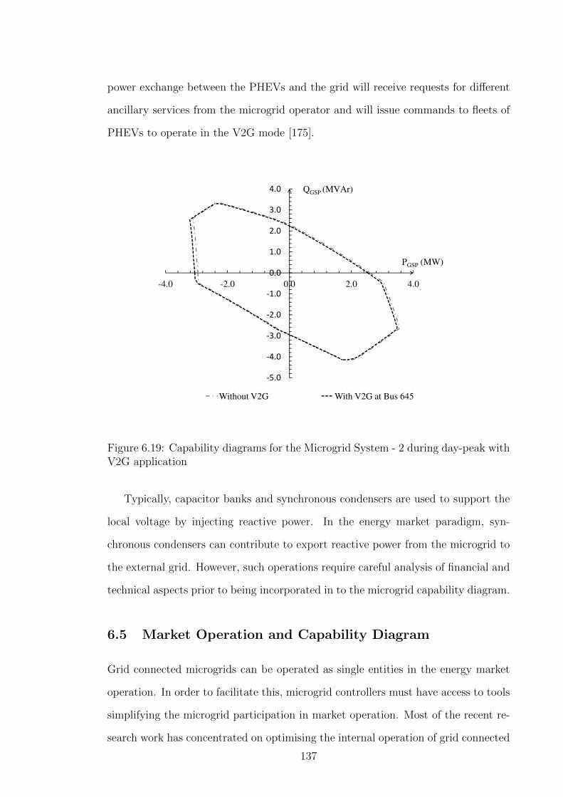
power exchange between the PHEVs and the grid will receive requests for different

ancillary services from the microgrid operator and will issue commands to fleets of

PHEVs to operate in the V2G mode [175].

-1.0

0.0

1.0

2.0

3.0

4.0

-4.0 -2.0 0.0 2.0 4.0

QGSP

(MVAr)

PGSP

(MW)

-5.0

-4.0

-3.0

-2.0

Without V2G With V2G at Bus 645

Figure 6.19: Capability diagrams for the Microgrid System - 2 during day-peak withV2G application

Typically, capacitor banks and synchronous condensers are used to support the

local voltage by injecting reactive power. In the energy market paradigm, syn-

chronous condensers can contribute to export reactive power from the microgrid to

the external grid. However, such operations require careful analysis of financial and

technical aspects prior to being incorporated in to the microgrid capability diagram.

6.5 Market Operation and Capability Diagram

Grid connected microgrids can be operated as single entities in the energy market

operation. In order to facilitate this, microgrid controllers must have access to tools

simplifying the microgrid participation in market operation. Most of the recent re-

search work has concentrated on optimising the internal operation of grid connected

137

microgrids either by minimising system losses or by minimising the power exchange

with the external grid [97, 99, 176–178]. However, as explained in Chapter 2, no re-

search work has suggested the use of a graphical tool for market operation of grid

connected microgrids. From various market operation strategies presented in Chap-

ter 2, this section presents two different case studies explaining the use of microgrid

capability diagram in market operation as a guideline for future work.

6.5.1 Active Power Exchange with the External Grid

The Microgrid System - 2 described in Section 6.3.2 is considered in these studies, to-

gether with the optimisation model developed as described in Section 6.3 considering

the limitations of the DGs, local loads, transformers and other network parameters.

For the particular microgrid, it is assumed that the microgrid is owned and con-

trolled by the MCC hence, DGs would not bid separately in the energy market.

The MCC would send relevant command signals to the DGs and no demand side

bidding is considered.

The microgrid operating cost includes the cost of main grid energy transac-

tions (both purchasing and selling), cost of microgrid energy supply, revenue from

local consumers, and any curtailment costs. The corresponding active and reactive

power capability diagram at 8.00 p.m. is illustrated in Fig. 6.20. Table 6.3 presents

the costs associated with the each DG operation and active power buying and selling

prices of the external grid.

Table 6.3: Costs associated with the microgrid operation

Cost ($/kWh)

Average cost of DFIG (DG1, DG2) [179,180] 0.063Average cost of small hydro (DG3) [181] 0.055

Active power buying and selling price of the external grid [182] 0.20

The microgrid would sell excess active power from the DGs to the external

grid when operating in the positive active power region of the capability diagram.

Whereas, in the negative active power region, microgrid would purchase active power

138

-5.0

-4.0

-3.0

-2.0

-1.0

0.0

1.0

2.0

3.0

4.0

-3.0 -2.0 -1.0 0.0 1.0 2.0 3.0 4.0

QGSP (MVAr)

PGSP (MW)

Figure 6.20: Capability diagram for the Microgrid System - 2 at 8.00 p.m.

from the external grid to fulfill the local load demand. For this scenario, it is assumed

that no cost is involved with the reactive power exchange between the microgrid and

the external grid. Thus, depending on the operation mode, the cost of electricity of

the microgrid is calculated using (6.25) and (6.26).

Active power export mode:

Electricity cost ($/kWh) =

∑DGcost∑PDG

(6.25)

Active power import mode:

Electricity cost ($/kWh) =Ext.grid purchase cost+

∑DGcost

Pext.grid +∑PDG

(6.26)

where,∑DGcost is the total cost of DG operation per hour,

∑PDG is the total

active power supplied from the DGs, and Pext.grid is the active power imported from

the external grid.

Analysing Fig. 6.20 and Fig. 6.21, it is clear that the electricity cost of the mi-

crogrid is around $ 0.06 /kWh during active power export mode. Furthermore, min-

imum cost of electricity occurs when there is no active power exchange between the

139

microgrid and the external grid (at PGSP = 0MW ). Cost of electricity reaches the

maximum of $ 0.20 /kWh when the total active power requirement of the microgrid

is met by the external grid. Fig. 6.22 illustrates the electricity cost variation of the

microgrid corresponding to all the operating points of the capability diagram.

0.00

0.05

0.10

0.15

0.20

0.25

-3.0 -2.0 -1.0 0.0 1.0 2.0 3.0 4.0PGSP (MW)

Microgrid electricity cost ($/kWh)

Figure 6.21: Electricity cost of the microgrid corresponding to the operating pointsof the boundary of the capability diagram

−4

−2

0

2

4

−3 −2 −1 0 1 2 3 4

0

0.05

0.10

0.15

0.20

0.25

QGSP

(MVAr)P

GSP (MW)

Mic

rogr

id e

lect

ricity

pric

e ($

/kW

h)

Figure 6.22: Electricity cost variation of the Microgrid System - 2 at 8.00 p.m.

140

6.5.2 Reactive Power Purchase from the External Grid

The microgrid system described in Section 6.5.1 is considered for this scenario. Apart

from the active power market, the MCC would be required to pay the external grid

for the reactive power imported into the microgrid. No cost is associated with

the reactive power export into the external grid. It is assumed that the MCC

purchase reactive power at a rate of $ 0.50 /kVArh. Fig. 6.23 illustrates the variation

of reactive power cost of the microgrid for reactive power import mode. As expected,

it can be observed that the cost of reactive power of the microgrid increases with

the increasing reactive power import from the external grid.

−2 −1 0 1 2 3 4−4−3

−2−1

0

−0.1

0

0.1

0.2

0.3

0.4

0.5

0.6

PGSP

(MW)QGSP

(MVAr)

$/kV

Ar

Figure 6.23: Variation of reactive power cost of the microgrid for reactive powerimport mode

In Section 6.5.1 and Section 6.5.2, only basic aspects of active and reactive power

markets were considered. However, depending on the ownership of the microgrid,

the market policy in operation can be varied. This would require many other aspects

to be considered when assigning cost values for different microgrid operating points.

A detailed discussion on this is presented in the following section.

141

6.6 Discussion

Due to time varying load and generation patterns, the capability diagram of a mi-

crogrid will vary with time and it is not practical for the MCC to derive capability

diagrams for an entire day. However, MCC can derive the capability diagrams for

pre-defined time periods or by using the forecasted generation and demand patterns

at critical operation times of the microgrid (i.e. day-peak, night-peak, minimum

load, and maximum generation). Furthermore, the capability diagram can be de-

rived online, provided proper communication media exists between the generators,

load centres and the MCC.

The proposed methodology and the mathematical model have the flexibility to

incorporate any optimisation algorithm and any constraint related to the micro-

grid for developing capability diagrams. DNSPs and MCCs can run optimisation

algorithms to optimise different objective functions subjected to different financial

and technical constraints. Regardless of the objective function, if all the technical

constraints are kept unchanged, those optimum operating points are located within

the microgrid capability diagram.

Through a capability diagram, the maximum possible power can be harnessed

from a grid connected microgrid. Furthermore, in a multi-microgrid environment

where microgrids trade between themselves, capability diagrams of individual mi-

crogrids can be used as a tool to decide the maximum amount of power exchange.

In this chapter, it was assumed that the microgrid was owned by an independent

power producer. Hence, the microgrid has the sole responsibility to cater the local

load demand either by generating power from local DGs or by importing power from

the utility (external grid). In such a situation, the microgrid owner has to bear the

expenses related to the electricity generation from DGs and energy purchase from

the external grid if any. The main revenue of the microgrid would be income derived

from selling energy into the external grid and to the local loads, with latter typically

providing larger return on investment.

However, if the local DGs have different owners, the MCC could allow the DGs

142

to bid in the energy market. In this scenario, apart from the aforementioned costs

associated with the energy generation, the MCC would have to bear the expenses

related to Lost Opportunity Costs. As an example, a decision to increase reactive

power export to the external grid would result in a reduction of active power pro-

duction from the local DGs. In this situation, MCC would be required to pay lost

opportunity cost to the relevant DGs, and buy active power if required from the

external grid. The market conditions and the cost of productions determine the

value of opportunity cost [183,184].

LOC - Lost Opportunity Cost

LS - Load Shedding

MG - Microgrid

MCC - Microgrid Central Controller

DG - Distributed Generator

P, Q

$

Active and reactive power flow

Money flow

Utiliy

MGiMGj

Reactive

Power

Sources

ConsumersStorage

Devices

DGMCC

External Grid

P, QP, Q

P, Q$

$

$

P, Q$

$ (LOC)

Q$

P, Q$

P, Q$

$ (LS)

Figure 6.24: Different components associated with the market operation of gridconnected microgrids

The price of reactive power is strongly dependent on the location of production.

The cost of producing reactive power is much lower than that of active power,

because it does not involve fuel costs [185]. However, the capital cost of a reactive

compensator, especially generator and synchronous condensers, is remarkably high.

Accordingly, the pricing mechanism should include the capital cost associated with

these components.

143

Operation of the microgrid in energy market can be more complex when demand

side bidding is considered. The MCC has to optimise the operation of the microgrid

by considering the bids from both DGs and the loads. If consumers are willing to

shed loads, the MCC will be required to pay a curtailment fee which will contribute

to the microgrid operating costs.

Thus, main operating objective of the microgrid will depend on the ownership,

network complexity, time of operation, and other market aspects. However, tech-

nical feasibility limits a microgrid can be derived regardless of the complexity of

the microgrid structure by expanding the methodology presented in this chapter.

Furthermore, electricity costs can be assigned to every operating point of the micro-

grid capability diagram and can be utilised as a tool in market operation with the

external grid and when trading between multiple microgrids. Fig. 6.24 illustrates

the diagram corresponding to different components associated with the market op-

eration of grid connected microgrids.

6.7 Summary

This chapter presented a new systematic approach for developing an active and

reactive power capability diagram corresponding to the GSP of a microgrid, while

considering microgrid generation capabilities, local load demands and network con-

straints. An optimisation model was developed under various network constraints

and the solutions were plotted on a P-Q power plane to derive the capability limits

for two different microgrid systems. Various features such as different load mod-

elling aspects, individual generator limitations, and effects of plug-in hybrid electric

vehicles and reactive power devices were considered in developing the capability

diagram.

The optimisation model for the capability diagrams were derived in MATLAB

for two different microgrid models, which were validated using DIgSILENT Power-

Factory. This graphical representation of the active and reactive power capability

at the GSP can be utilised as a new tool to represent the technical feasibility of grid

144

connected microgrids when trading with the utility and other microgrids. The MCC

would be able to use the DERs optimally and to provide ancillary services support

to the external network as required.

This chapter introduced the use of microgrid capability diagram as a tool for the

market operation of grid connected microgrids. Two case studies were presented in

active and reactive power markets where electricity prices were assigned to every

operating point of the capability diagram. Such diagrams can be referred to by the

MCC in decision making processes.

145

Chapter 7

Low Voltage Ride Through of

Microgrids with Distribution

Static Synchronous

Compensator (DSTATCOM)

7.1 Introduction

Faults occurring outside a grid connected microgrid can lead to voltage sags at

the microgrid point of common coupling (PCC) which would propagate to affect

the operation of the distributed energy resources (DERs) and the loads within the

microgrid. If the DERs are set to disconnect at relatively shallow voltage sag depth

levels, a situation with considerable generation deficit can arise. However, such a

scenario can be avoided if the microgrid can regulate the voltage at the PCC and

provide dynamic reactive power support to the network during voltage sag events.

Depending on the low voltage ride through (LVRT) behaviour of individual DERs

within the microgrid, those DERs can also provide dynamic voltage and reactive

power support to the rest of the microgrid. As described in Chapter 2, research

outcomes exist related to the individual LVRT behaviour of DERs in compliance

146

to different grid codes. However, the collective effect of LVRT behaviour of DERs

within a microgrid has not been investigated so far.

This chapter takes two approaches in order to investigate the LVRT behaviour of

a grid connected microgrid as a single entity. First approach is to improve dynamic

voltage support at the microgrid PCC by using a distribution static synchronous

compensator (DSTATCOM) at the low voltage side of the microgrid distribution

transformer. The second approach is to use the aggregated reactive power capa-

bility of DERs within a microgrid to provide voltage and reactive power support

to the external grid. During this approach, instead of individual DG capabilities,

DSTATCOMs are installed at the DG terminals, and no additional dynamic voltage

support (i.e. DSTATCOM) is considered at low voltage side of the microgrid distri-

bution transformer. This chapter is exclusively focussed on the technical assessment

of DSTATCOM for microgrids and its advantage for grid connected and islanded

modes of operation.

Section 7.2 describes the voltage control mode of a DSTATCOM and selection

of the parameters in order to improve dynamic voltage support. The impact of

DSTATCOM in a grid connected microgrid under different operating conditions

is investigated in Section 7.3. The microgrid is subjected to external and internal

faults, and various system parameters are analysed with and without the DSTAT-

COM operation. DSTATCOMs are installed at DG terminals and at the bus bar

with minimum reactive power margin of the microgrid, and the system behaviour is

analysed in Section 7.4.

Integration of multiple microgrids into the utility grid will allow the microgrids

to provide ancillary services to the utility during normal operation and will enable

emergency services to adjacent microgrids during a utility grid outage. Maintaining

the microgrids online will avoid sudden loss of active power while avoiding power

system collapse. Section 7.5 presents DSTATCOM operation in a multi-microgrid

system which is investigated for different faults.

Operation of single microgrids in islanded mode and operation of multiple micro-

147

grids separated from external grid with DSTATCOMs are presented in Section. 7.6.

Section 7.7 presents a case study carried out to investigate grid connected microgrid

behaviour with DSTATCOM and induction motor loads followed by the chapter

summary in Section 7.8.

7.2 Distribution Static Synchronous Compensator (DSTAT-

COM)

DSTATCOM is a shunt reactive power compensating device which functions as a

controlled shunt reactive admittance and generates ac voltage, which in turn causes a

current injection into the system through a shunt transformer. In its most basic form,

the DSTATCOM configuration consists of a two-level voltage source inverter (VSI),

a dc energy storage device, a coupling transformer connected in shunt with the ac

system, and associated control circuits as illustrated in Fig. 7.1 [186].

DSTATCOM

Cdc

Vdc

Lf

Vt

T/f

Figure 7.1: General topology of a VSI based DSTATCOM [167]

The VSI converts the dc voltage across the storage device into three-phase ac

voltages. These voltages are synchronised with the ac system through the reactance

of the coupling transformer. Suitable adjustments of the phase and magnitude of

the DSTATCOM output voltage allow effective control of active and reactive power

exchange between the DSTATCOM and the ac system. The VSI connected in shunt

with the ac system provides a multi-functional topology which can be used for up

148

to three quite distinct purposes: 1) voltage regulation and compensation of reactive

power, 2) correction of power factor, 3) elimination of current harmonics.

Fig. 7.2 illustrates the controller associated with the voltage control mode of the

DSTATCOM. In voltage control mode, the difference between the RMS voltage of

the terminal and its desired value is used to generate the required voltage magnitude

across the filter by exchanging reactive power with the ac network. The droop is

usually selected as 5 % to allow small terminal voltage variations while avoiding

oscillation [187]. The dc voltage is kept constant through a small active power

exchange arrangement with the ac network, which also compensates for the active

power losses in the transformer and the inverter.

abc→ dq

PLL

PI

Droop

PI

Inverter

PI

PI

Vabc

Iabc

Vrms

Φ

Vrms-ref

Iq-ref

Id

Iq

Id-ref

Vdc

Vdc-ref

Vq

Vd

+

+

+

+

-

-

-

-

Vabc

Figure 7.2: DSTATCOM voltage control mode

7.2.1 Design of DSTATCOM Parameters

Reference dc Link Voltage (Vdcref)

In order to achieve good tracking performance, voltage across the dc storage capac-

itor is selected to be 1.6Vm, where Vm is the maximum phase voltage [188].

149

Storage Capacitance (Cdc)

Value of the dc capacitor is selected based on the ability to regulate voltage during

transients. During transients, the dc capacitor exchanges real power to maintain

the load power demand. Assuming the controller starts working after n cycles, nST

would be the maximum possible energy that the capacitor can exchange with the

load, where S is the maximum load rating, and T is system time period [189]. Hence,

1

2Cdc(V

2dcref − V 2

dc) = nST (7.1)

where, Vdc is the magnitude of the maximum allowed voltage deviation from Vdcref

during transients. Therefore, the dc link capacitor value is selected as follows:

Cdc =2nST

V 2dcref − V 2

dc

(7.2)

Interfacing Inductance (Lf)

The inductor is designed to provide good tracking performance at maximum switch-

ing frequency. Neglecting filter resistanceRf , interfacing inductance is given by,

Lf =Vdcref

(2h)(2fmax)(7.3)

where, 2h is the ripple in the current and fmax is the maximum switching frequency

achieved using a hysteresis current controller [189].

7.3 Grid Connected Microgrid in Different Operating Re-

gions with DSTATCOM

In this section, different case studies are carried out to investigate the impact of

having a DSTATCOM at the secondary side of the coupling transformer of a grid

connected microgrid. Fig. 7.3 illustrates the microgrid system developed for the case

studies where DG1 and DG2 represent DFIGs, while DG3 represents a SG based

150

DG. Both DG1 and DG2 are operated in constant power factor mode while DG3 is

operated in voltage control mode.

Bus 650

DG 1

Bus 680

DG 2

DG 3

Bus 646 Bus 645 Bus 632

Bus 611 Bus 684

Bus 652

Bus 671 Bus 692

Bus 633

Bus 675

Bus634

External

grid

0.69 kV 0.69 kV

4.16 kV

115 kV

Bus 632-1

Figure 7.3: Single line diagram of the microgrid system

Q (MVAr)

P (MW)

R1

R4R3

R2

+

+

Figure 7.4: Microgrid operating regions for grid connected mode

Fig. 7.4 illustrates the four different microgrid operating regions considered in

this section, where positive power values indicate power export from the microgrid.

Table 7.1 presents the active and reactive power flow from DGs, the external grid

and the total microgrid load demand considered in this section related to the four

operating regions.

151

Tab

le7.

1:A

ctiv

ean

dre

acti

vep

ower

valu

esfo

rdiff

eren

top

erat

ing

regi

ons

ofth

em

icro

grid

R1

R2

R3

R4

P(M

W)

Q(M

VA

r)P

(MW

)Q

(MV

Ar)

P(M

W)

Q(M

VA

r)P

(MW

)Q

(MV

Ar)

DG

11.

200

00

00.

276

0.76

91.

100

0.50

0D

G2

1.20

00

00

0.23

10.

962

0.90

00

DG

34.

000

-1.8

404.

000

0.50

71.

527

0.49

91.

500

0.68

7E

xt.

Gri

d3.

575

-3.7

92-0

.711

-1.6

03-0

.677

0.61

72.

033

0.27

2T

otal

load

2.27

11.

293

4.55

21.

932

2.68

31.

563

1.39

40.

803

152

7.3.1 Microgrid Behaviour during an External Fault with DSTAT-

COM

For the microgrid considered in this study, a 3 MVA DSTATCOM is selected, and

the parameters calculated as explained in Section 7.2.1 are presented in Table 7.2.

Table 7.2: Parameters of the DSTATCOM

Parameter Value Parameter Value

Cdc 4629µF n 0.5Vdcref 6 kV T 0.02 sLf 150 mH h 1 AVac 4.16 kV fmax 10 kHz

9 10 11 12 13 14 15−4

−2

0

2

P DS

TA

TC

OM (

MW

)

(a)

R1 R2 R3 R4

9 10 11 12 13 14 15−2

0

2

QD

ST

AT

CO

M (M

VA

r)

(b)Time (s)

R1 R2 R3 R4

Figure 7.5: Active and reactive power variations of the DSTATCOM in differentoperating regions of the microgrid (fault duration for R1-538 ms, R2, R3 and R4 -160 ms)

In order to investigate the impact of the DSTATCOM connected on low voltage

153

side of the microgrid distribution transformer, a three-phase short-circuit fault was

applied to Bus bar 650 at t = 10 s and cleared after 160 ms to the microgrid. The

study is carried out on all four operating regions of the microgrid.

9 10 11 12 13 14 15 16 17 18 19 20

0

0.2

0.4

0.6

0.8

1

X: 10.4Y: 0.1719

Vol

tage

(pu

)

(a)

X: 10.41Y: 0.3365

650 632 646 633 675

9 10 11 12 13 14 15 16 17 18 19 200

0.2

0.4

0.6

0.8

1

X: 10.4Y: 0.1999

Vol

tage

(pu

)

X: 10.41Y: 0.3585

(b)Time (s)

650 632 646 633 675

Figure 7.6: Voltage variations at different bus bars in operating region R1 (a) withoutDSTATCOM and (b) with DSTATCOM (fault duration - 538 ms)

Table 7.3: CCT of the microgrid for different operating regions

Operating region Without DSTATCOM (ms) With DSTATCOM (ms)

R1 538 632R2 298 331R3 196 218R4 188 221

Fig. 7.5 (a) and Fig. 7.5 (b) illustrate the active and reactive power variations of

the DSTATCOM in the four different microgrid operating regions due to the fault.

The DSTATCOM injected reactive power into the network during the fault and after

fault clearance in order to maintain the terminal voltage at the pre-fault value. The

154

i===

I\~

11

- rr

\.1 ' · _j

9 10 11 12 13 14 150

0.2

0.4

0.6

0.8

1

X: 10.12Y: 0.1787

Vol

tage

(pu

)

(a)

X: 10.12Y: 0.424

650 632 646 633 675

9 10 11 12 13 14 150

0.2

0.4

0.6

0.8

1

X: 10.12Y: 0.2086

Vol

tage

(pu

)

X: 10.12Y: 0.449

(b)Time (s)

650 632 646 633 675

Figure 7.7: Voltage variations at different bus bars in operating region R2 (a) withoutDSTATCOM and (b) with DSTATCOM (fault duration - 160 ms)

9 10 11 12 13 14 150

0.2

0.4

0.6

0.8

1

X: 10.12Y: 0.2265

Vol

tage

(pu

)

Time (s)

X: 10.12Y: 0.4522

650 632 646 633 675

Figure 7.8: Voltage variations at different bus bars in operating region R3 withoutDSTATCOM (fault duration - 160 ms)

critical clearing time (CCT) of the three-phase short-circuit fault was determined

for each operating region of the microgrid with and without the DSTATCOM. The

CCT for the microgrid was determined based on the SG pole slip, and any grid code

155

compliance or the action of protection devices were not taken into consideration. It

can be observed from Table 7.3 that the CCT of the microgrid with DSTATCOM is

longer compared to the microgrid without the DSTATCOM. Therefore, provision of

reactive power support from the DSTATCOM has enabled the microgrid to operate

over a longer period during a fault.

9 10 11 12 13 14 150

0.2

0.4

0.6

0.8

1

X: 10.12Y: 0.249

Vol

tage

(pu

)

X: 10.12Y: 0.4726

Time (s)

650 632 646 633 675

Figure 7.9: Voltage variations at different bus bars in operating region R3 withDSTATCOM (fault duration - 160 ms)

Fig. 7.6 (a) and Fig. 7.6 (b) illustrate the voltage variations of five of the bus

bars in the microgrid without and with the DSTATCOM for a fault duration of

538 ms. Comparing those figures, it can be observed that the post fault voltage has

improved considerably with the DSTATCOM. Furthermore, depth of the voltage

sag has decreased by 0.022 pu during the fault with the DSTATCOM for operating

region R1. Fig. 7.7 illustrates the variation of voltage for operating region R2, which

indicates approximately a 0.03 pu decrease in the voltage sag during the fault with

the DSTATCOM. Similarly, for operating regions R3 and R4, an improvement of

the depth of the voltage sag can be noted with the DSTATCOM, as observed from

Fig. 7.8 to Fig. 7.10 respectively.

Fig. 7.11 illustrates the reactive power variations of the distribution lines con-

nected to Bus bar 632 with the DSTATCOM. In operating region R1, reactive power

has flowed from the distribution transformer to the microgrid during steady state.

During the fault, it can be observed that the direction of the reactive power flow has

156

9 10 11 12 13 14 150

0.2

0.4

0.6

0.8

1

X: 10.12Y: 0.248

Vol

tage

(pu

)

(a)

X: 10.12Y: 0.4855

650 632 646 633 675

9 10 11 12 13 14 150

0.2

0.4

0.6

0.8

1

X: 10.12Y: 0.2774

Vol

tage

(pu

)

X: 10.12Y: 0.5106

(b)Time (s)

650 632 646 633 675

Figure 7.10: Voltage variations at different bus bars in operating region R4(a) without DSTATCOM and (b) with DSTATCOM (fault duration - 160 ms)

changed from the microgrid to the distribution transformer. With the DSTATCOM,

maximum reactive power variation of the microgrid during the fault has increased

by 0.8 MVAr. Furthermore, post fault transients are considerably less and system

reached the steady state faster with the DSTATCOM in the microgrid. Similar to

operating region R1, reactive power has been imported into the microgrid in operat-

ing region R2 at steady state. From Fig. 7.12, it can be observed that reactive power

contribution from the microgrid has increased during the fault due to the DSTAT-

COM operation as well as reduction in post fault transients. By examining Fig. 7.13

to Fig. 7.15 corresponding to the operation of regions R1 and R2 of the microgrid,

it can be identified that the reactive current contribution from the microgrid into

the external grid during the fault has increased due to the reactive power supplied

by the DSTATCOM.

157

10 15 20 25−15

−10

−5

0

5

X: 10.61Y: −11.5

Qlin

e (M

VA

r)

(a)

X: 10.01Y: 4.106

632~632−1 632~633 632~645 632~671

10 15 20 25−15

−10

−5

0

5

X: 10.61Y: −8.26

Qlin

e (M

VA

r)

X: 10.01Y: 4.897

(b)Time (s)

632~632−1 632~633 632~645 632~645

Figure 7.11: Reactive power flow variations in the distribution lines connected toBus bar 632 (R1) (a) without DSTATCOM operation and (b) with DSTATCOMoperation due to an external grid fault

Fig. 7.16 and Fig. 7.17 illustrate the variations of reactive power flow of the dis-

tribution lines connected to Bus bar 632 with the DSTATCOM in operating regions

R3 and R4 respectively, in which reactive power has been exported to the external

grid. Observing those figures, it can be identified that the maximum reactive power

flow from the microgrid into the distribution transformer has increased by 1.6 MVAr

with the DSTATCOM. Similarly, with the DSTATCOM, approximately 1.0 MVAr of

reactive power increase can be observed in operating region R4. With the DSTAT-

COM, less post fault transients can be observed in the microgrid. By examining

Fig. 7.18, Fig. 7.19, and Fig. 7.20 corresponding to the operating regions R3 and R4

of the microgrid, it can be identified that the reactive current contribution from the

microgrid into the external grid has increased due to the connection of the DSTAT-

158

~" \

~ "----- ~~- -=-~- -=--~-~- -=-=--=-~- -=-=--=-=- -=-=--=--~-~- -= -=- -=--~-~- -=-=--=-=--=-=- ~-~- -=-=--=-=--=-~- -=--~-~- =-=-=--=--~-~- -=-=--=-=- -~-

I---~~:___--- -_--------_-------_--------_--------_--------_______,-------

\/

9 10 11 12 13 14 15−4

−3

−2

−1

0

1

2

3

4

X: 10.01Y: 2.431

Qlin

e (M

VA

r)

(a)

X: 10.17Y: −2.182

632~632−1 632~633 632~645 632~671

9 10 11 12 13 14 15−4

−3

−2

−1

0

1

2

3

4

X: 10.01Y: 3.088

Qlin

e (M

VA

r)

(b)Time (s)

632~632−1 632~633 632~645 632~675

Figure 7.12: Reactive power flow variations in the distribution lines connected toBus bar 632 (R2) (a) without DSTATCOM operation and (b) with DSTATCOMoperation due to an external grid fault

10 15 20 25−4

−3

−2

−1

0

1

2

3

X: 10.01Y: 2.398

Rea

ctiv

e cu

rren

tlin

e (pu

)

Time (s)

632~632−1 632~633 632~645 632~671

Figure 7.13: Reactive current flow in the distribution lines connected to Bus bar632 (R1) without DSTATCOM operation due to an external grid fault

COM. Therefore, it is clear that a DSTATCOM can be used to provide additional

reactive power during faults in order to improve post fault voltage recovery of the

159

I\

.. . . '

'' . ' . ' ' ' . : . . .

' ' .. ,,

.. ~---- .... ----------- --~---------------------

,,

Ill

r------11---1 ~\~~-._,/--~-------------=--------~---------------------------------------=--------' ' ' ' ' ' ' ' '' ..

i ["

10 15 20 25−3

−2

−1

0

1

2

3

X: 10.01Y: 2.618

Rea

ctiv

e cu

rren

tlin

e (pu

)

Time (s)

632~632−1 632~633 632~645 632~671

Figure 7.14: Reactive current flow in the distribution lines connected to Bus bar632 (R1) with DSTATCOM operation due to an external grid fault

9 10 11 12 13 14 15−1

−0.5

0

0.5

1

1.5

X: 10.01Y: 1.46

Rea

ctiv

e cu

rren

tlin

e (pu

)

(a)

632~632−1 632~633 632~645 632~671

9 10 11 12 13 14 15−0.5

0

0.5

1

1.5

2X: 10.01Y: 1.63

Rea

ctiv

e cu

rren

tlin

e (pu

)

(b)Time (s)

632~632−1 632~633 632~645 632~671

Figure 7.15: Reactive current flow in the distribution lines connected to Bus bar632 (R2) (a) without DSTATCOM operation and (b) with DSTATCOM operationdue to an external grid fault

microgrid.

160

9 10 11 12 13 14 15

−4

−2

0

2

4

6

X: 10.17Y: −2.561

Qlin

e (M

VA

r)

(a)

X: 10.01Y: 4.517

632~632−1 632~633 632~645 632~671

9 10 11 12 13 14 15−8

−6

−4

−2

0

2

4

6

8

X: 10.17Y: −1.621

Qlin

e (M

VA

r)

X: 10.01Y: 6.162

(b)Time (s)

632~632−1 632~633 632~645 632~671

Figure 7.16: Reactive power flow variations in the distribution lines connected toBus bar 632 (R3) due to an external grid fault

7.3.2 Microgrid Behaviour due to Internal Faults with DSTATCOM

In order to analyse the effect of DSTATCOM due to internal faults, different faults

were applied at three different bus bars in the microgrid when operating in region

R1. The DSTATCOM was kept connected to Bus bar 632. Three-phase short-

circuit faults were applied to Bus bars 611, 633 and 692 through different fault

impedances. Fig. 7.21 illustrates the magnitude of the minimum voltage measured

at the DSTATCOM terminal during three different faults. It can be observed that

during voltage sag, the minimum voltage has improved due to the DSTATCOM

operation. Fig. 7.22 illustrates the reactive power injected by the DSTATCOM into

the network during microgrid internal faults. Depending on the severity at the

DSTATCOM terminal, reactive power support is provided by the DSTATCOM to

the microgrid system.

161

b.

:: _r r<~-- ·~:::: __ -._:.:::":.:: ....... : ::::::::::::::::::: ::::::::::::::::::::

' ' ' ' ~ : ' ' ',_.'

,' .. ~-- ---------- ... ----------

l

9 10 11 12 13 14 15−6

−4

−2

0

2

4

6

X: 10.17Y: −1.746

Qlin

e (M

VA

r)

(a)

X: 10.01Y: 5.22

632~632−1 632~633 632~645 632~671

9 10 11 12 13 14 15−8

−6

−4

−2

0

2

4

6

8

X: 10.01Y: 6.326

Qlin

e (M

VA

r)

(b)Time (s)

632~632−1 632~633 632~645 632~671

Figure 7.17: Reactive power flow variations in the distribution lines connected toBus bar 632 (R4) due to an external grid fault

9 10 11 12 13 14 15−1

−0.5

0

0.5

1

1.5

2

X: 10.01Y: 1.972

Rea

ctiv

e cu

rren

tlin

e (pu

)

Time (s)

632~632−1 632~633 632~645 632~671

Figure 7.18: Reactive current flow in the distribution lines connected to Bus bar632 (R3) without DSTATCOM operation due to an external grid fault

7.4 Impact of DSTATCOM Location in the Microgrid

7.4.1 DSTATCOM Connection at DG Terminals

In this section, the DSTATCOM on the secondary side of the distribution trans-

former was removed from the bus bar in the microgrid system introduced in Sec-

162

- -~ - ~ - - - ---- --

9 10 11 12 13 14 15−1

−0.5

0

0.5

1

1.5

2

2.5

X: 10.01Y: 2.303

Rea

ctiv

e cu

rren

tlin

e (pu

)

Time (s)

632~632−1 632~633 632~645 632~671

Figure 7.19: Reactive current flow in the distribution lines connected to Bus bar632 (R3) with DSTATCOM operation due to an external grid fault

9 10 11 12 13 14 15−1

−0.5

0

0.5

1

1.5

2

X: 10.01Y: 2.12

Rea

ctiv

e cu

rren

tlin

e (pu

)

(a)

632~632−1 632~633 632~645 632~671

9 10 11 12 13 14 15−1

−0.5

0

0.5

1

1.5

2

2.5

X: 10.01Y: 2.333

Rea

ctiv

e cu

rren

tlin

e (pu

)

(b)Time (s)

632~632−1 632~633 632~645 632~671

Figure 7.20: Reactive current flow in the distribution lines connected to the DSTAT-COM (R4) (a) without DSTATCOM operation and (b) with DSTATCOM operationdue to an external grid fault

tion 7.3, and two DSTATCOMs were connected at the two terminals of DG1 and

DG2. In order to compare the results with those of Section. 7.3, aggregated gen-

163

611 633 6920

0.1

0.2

0.3

0.4

0.5

0.6

0.7

0.8

Sag

dept

h at

Bus

632

(pu

)

Fault location

With DSTATCOM Without DSTATCOM

Figure 7.21: Magnitude of the voltage sag depth at Bus bar 632 for different internalfaults with and without DSTATCOM

9 10 11 12 13 14 15 16 17 18 19 20−0.5

0

0.5

1

1.5

2

2.5

3

QD

ST

AT

CO

M (M

VA

r)

Time (s)

611 633 692

Figure 7.22: Reactive power output of the DSTATCOM for different internal faultsin the microgrid

erator capacity was maintained at 3 MVA, hence each DSTATCOM was rated at

1.5 MVA. DG3 was assumed to be disconnected in the microgrid and the different

operating conditions considered for this case study are presented in Table 7.4. A

three-phase short-circuit fault was applied at Bus bar 650 at t = 10 s and cleared

after 160 ms.

Fig. 7.23 and Fig. 7.24 illustrate the voltage variations of five bus bars in the

microgrid due to the fault. As a result of the fault, terminal voltages of both

DG1 and DG2 are zero, and the crowbar protection in both DG1 and DG2 were

activated at 10.013 s and deactivated at 10.080 s. However, with the DSTATCOM

operation, voltage profile of the microgrid has improved during the fault and the

164

Table 7.4: Power flow levels of the microgrid

P (MW) Q (MVAr)

DG1 0.900 0.0DG2 0.900 0.0

Ext.grid 0.161 1.101Total load 1.923 1.042

9 9.5 10 10.5 11 11.5 120

0.2

0.4

0.6

0.8

1

Vol

tage

(pu

)

(a)

650 632 646 633 652

9 9.5 10 10.5 11 11.5 120

0.2

0.4

0.6

0.8

1

X: 10.03Y: 0.06217

Vol

tage

(pu

)

(b) Time (s)

650 632 646 633 652

Figure 7.23: Voltage variations (a) without DSTATCOM and (b) with DSTATCOMconnected at Bus bar 632 (fault at Bus bar 650)

crowbar protection was not activated as illustrated in Fig. 7.23 (b), and has allowed

the DGs to supply power to the microgrid without any interruption. However, it

has a less positive effect on the voltage profile compared to the case of having the

DSTATCOM on low voltage side of the microgrid distribution transformer.

Fig. 7.25 and Fig. 7.26 present the reactive power flow through the distribution

lines connected to Bus bar 632. By examining these figures, it can be observed that

having a DSTATCOM on the low voltage side of the microgrid distribution trans-

165

9 9.5 10 10.5 11 11.5 120

0.2

0.4

0.6

0.8

1

X: 10.03Y: 0.05376

Vol

tage

(pu

)

Time (s)

650 632 646 633 652

Figure 7.24: Voltage variations with two DSTATCOMs at DG1 and DG2 termi-nals (fault at Bus bar 650)

9 9.5 10 10.5 11 11.5 12−6

−4

−2

0

2

4

X: 10.17Y: −5.392

Qlin

e (M

VA

r)

(a)

X: 10.15Y: 0.1548

X: 10.01Y: 0.8789

632~632−1 632−633 632−645 632−671

9 9.5 10 10.5 11 11.5 12−6

−4

−2

0

2

4

X: 10.15Y: 0.3983

Qlin

e (M

VA

r)

X: 10.17Y: −4.685

X: 10.01Y: 1.545

(b)Time (s)

632~632−1 632~633 632~645 632~671

Figure 7.25: Reactive power variations of the distribution lines connected to Busbar 632, (a) without DSTATCOM and (b) with DSTATCOM connected at Bus bar632 (fault at Bus bar 650)

former would increase the reactive power flow towards the distribution transformer.

Furthermore, during the post fault transients, reactive power absorption from the

166

9 9.5 10 10.5 11 11.5 12−8

−6

−4

−2

0

2

4

X: 10.01Y: 1.499

Qlin

e (M

VA

r)

Time (s)

X: 10.17Y: −6.122

632~632−1 632−633 632−645 632−671

Figure 7.26: Reactive power variations of the distribution lines connected to Busbar 632 with two DSTATCOMs at DG1 and DG2 terminals (fault at Bus bar 650)

9 9.5 10 10.5 11 11.5 12−1

−0.5

0

0.5

1

X: 10.01Y: 0.8697

Rea

ctiv

e cu

rren

tlin

e (pu

)

(a)

X: 10.17Y: −0.8747

X: 10.11Y: 0.4049

632~632−1 632−633 632−645 632−671

9 9.5 10 10.5 11 11.5 12−1

−0.5

0

0.5

1

1.5

X: 10.11Y: 0.6239

Rea

ctiv

e cu

rren

tlin

e (pu

)

X: 10.17Y: −0.7952

X: 10.01Y: 1.153

(b)Time (s)

632~632−1 632~633 632~645 632~675

Figure 7.27: Reactive current flow of the distribution lines connected to Bus bar632 (a) without DSTATCOM and (b) with DSTATCOM connected at Bus bar 632(fault at Bus bar 650)

167

microgrid was minimum when the DSTATCOM was installed on the low voltage

side of the microgrid distribution transformer.

9 9.5 10 10.5 11 11.5 12−1.5

−1

−0.5

0

0.5

1

1.5

X: 10.01Y: 1.136

Rea

ctiv

e cu

rren

tlin

e (pu

)

Time (s)

X: 10.17Y: −1.094

X: 10.11Y: 0.558

632~632−1 632−633 632−645 632−671

Figure 7.28: Reactive current flow of the distribution lines connected to Bus bar 632with two DSTATCOMs at DG1 and DG2 terminals (fault at Bus bar 650)

As illustrated in Fig. 7.27, reactive current flow from the microgrid into the ex-

ternal grid has significantly increased due to the operation of the DSTATCOM.

Compared to the operation of DSTATCOMs at the DG terminals, a DSTATCOM

near the secondary side of the microgrid distribution transformer has better reac-

tive current contribution to the external grid during the fault. Furthermore, by

examining Fig. 7.27 and Fig. 7.28, it can be observed that the post fault reactive

current flow into the microgrid is high when the DSTATCOMs are connected at DG

terminals.

7.4.2 DSTATCOM Connection at the Bus bar with Minimum Reac-

tive Power Margin of the Microgrid

In this section, the DSTATCOM was connected at the bus bar with the minimum

reactive power margin of the microgrid in order to investigate the impact of DSTAT-

COM location on microgrid performance during faults. The same microgrid system

described in Section 7.4.1 was used for this case study, and for the purpose of com-

parison, rating of the DSTATCOM was selected to be 3 MVA. In order to find the bus

bar with the minimum reactive power margin in the microgrid, V-Q curve method

168

Q_margin

0

+Q (MVAr)

-Q

V (pu)

dQ/dV =0

Figure 7.29: V-Q curve and reactive power margin

611 632 633 645 646 652 671 675 680 684 6920

5

10

15

20

Rea

ctiv

e po

wer

mar

gin

(MV

Ar)

Bus

Figure 7.30: Reactive power margins of the bus bars in the microgrid

was used in this section. V-Q curves were used to determine the capability of a bus

bar to maintain voltage during normal and abnormal conditions [190]. Minimum

of the V-Q curve (where dQ/dV = 0) represents the voltage stability limit, where

the distance of the operating point at any particular loading to the minimum of

the curve gives an indication to the closeness of system collapse [191]. V-Q curves

were derived through a series of ac power flow solutions, and the reactive power

margin (Q margin) was measured as the distance between the reactive power level

of the V-Q curve at dQ/dV = 0 and the voltage axis as illustrated in Fig. 7.29. A

positive reactive power margin indicates a deficit of reactive power at the particular

bus bar whereas, a negative reactive power margin indicates the amount of reactive

169

power the bus bar can supply to the system without being unstable.

Fig. 7.30 illustrates the reactive power margins of the bus bars in the microgrid,

and Bus bar 652 was identified as the bus bar the minimum reactive power margin.

9 9.5 10 10.5 11 11.5 120

0.2

0.4

0.6

0.8

1

X: 10.03Y: 0.1159

Vol

tage

(pu

)

Time (s)

650 632 646 633 652

Figure 7.31: Voltage variations with a DSTATCOM at the bus bar with minimumQ-margin (fault at Bus bar 650)

9 9.5 10 10.5 11 11.5 12−8

−6

−4

−2

0

2

4

X: 10.17Y: −6.285

Qlin

e (M

VA

r)

Time (s)

X: 10.01Y: 1.526

632~632−1 632−633 632−645 632−671

Figure 7.32: Reactive power variations of the distribution lines connected to Busbar 632 with DSTATCOM connected at the bus bar with minimum Q-margin (faultat Bus bar 650)

The microgrid was subjected to the same three-phase short-circuit fault consid-

ered in Section 7.4.1, and Fig. 7.31 presents the voltage variations of the bus bars

due to the fault. As expected, it can be observed that the voltage profile of the

bus bar connected to the DSTATCOM has improved. Comparing Fig. 7.25 (b)

and Fig. 7.27 (b) with Fig. 7.32 and Fig. 7.33, it can be observed that installing a

DSTATCOM near the distribution transformer of the microgrid has provided better

170

9 9.5 10 10.5 11 11.5 12−1.5

−1

−0.5

0

0.5

1

1.5

X: 10.11Y: 0.5755

Rea

ctiv

e cu

rren

tlin

e (pu

)

Time (s)

X: 10.17Y: −1.113

X: 10.01Y: 1.146

632~632−1 632−633 632−645 632−671

Figure 7.33: Reactive current flow variations of the distribution lines connected toBus bar 632 with a DSTATCOM connected at the bus with minimum Q-margin(fault at Bus bar 650)

reactive power performance when the microgrid was subjected to faults. When the

DSTATCOM was not installed on the low voltage side of the microgrid distribu-

tion transformer, the microgrid was unable to utilise the maximum capability of the

DSTATCOM to provide support to the external grid.

Fig. 7.34 (a) and Fig. 7.34 (b) illustrate the reactive power output variations of

DG1 and DG2 for different DSTATCOM locations. It can be observed that instal-

lation of a DSTATCOM in the microgrid has allowed the DGs to provide reactive

power into the microgrid continuously without being interrupted by the activation

of crowbar protection as explained in Section 7.4.1. Fig. 7.34 (c) illustrates the to-

tal reactive power contribution from the DSTATCOMs installed in the microgrid.

Reactive power output from the two DSTATCOMs installed at the DG terminals

were added together for comparison (as both DSTATCOMs were rated at 1.5 MVA).

Analysing the post fault behaviour, it can be observed that when the DSTATCOMs

are installed on the low voltage side of the microgrid distribution transformer and

at the DG terminals, they provide better reactive power contribution compared to

the DSTATCOM at the bus bar with the minimum reactive power margin. Fig. 7.35

summarises the minimum voltage levels experienced by the bus bars in the microgrid

during the fault with and without DSTATCOM operation. From a careful analysis,

it can be concluded that having the DSTATCOM installed on the low voltage side

171

9.5 10 10.5 11 11.5 12−2.5

−2

−1.5

−1

−0.5

0

0.5

1

1.5

QD

G1 (

MV

Ar)

(a)

without DSTATCOM At Bus−632 At DG terminals At Bus−652

9.5 10 10.5 11 11.5 12−2.5

−2

−1.5

−1

−0.5

0

0.5

1

1.5

QD

G2 (

MV

Ar)

(b)

without DSTATCOM At Bus−632 At DG terminals At Bus−652

9.5 10 10.5 11 11.5 12−2

−1

0

1

2

3

QD

ST

AT

CO

M (M

VA

r)

(c)Time (s)

At Bus−632 At DG1 terminal At DG2 terminal At Bus−652

Figure 7.34: Variation of reactive power contribution of (a) DG1, (b) DG2, and(c) DSTATCOM with different DSTATCOM locations (fault at Bus bar 650)

of the microgrid distribution transformer has better impact on all the bus bars of

the microgrid compared to the DSTATCOM installed at other locations studied.

172

" " .

611 632 633 634 645 646 650 652 671 675 680 684 692 632−10

0.01

0.02

0.03

0.04

0.05

0.06

0.07

0.08

0.09

Vm

inim

um (

pu)

Bus

Without DSTATCOM At Bus 632 At DG terminals At Bus 652

Figure 7.35: Minimum voltage of microgrid bus bars during the fault at Bus bars650

External

grid

Bus 650

MG 2MG 1

115 kV

4.16 kV

MG 3

4.16 kV 4.16 kV

Figure 7.36: Multi-microgrid system

9 10 11 12 13 14 15−15

−10

−5

0

5

X: 10.17Y: −6.477

Rea

ctiv

e po

wer

(M

VA

r)

Time (s)

X: 10.17Y: −11.66

Without DSTATCOM With DSTATCOM

Figure 7.37: Reactive power exchange with the external grid with and withoutDSTATCOM in each microgrid (fault at Bus bar 650)

173

Table 7.5: Operating conditions of the microgrids

MG1 MG2 MG3P (MW) Q (MVAr) P (MW) Q (MVAr) P (MW) Q (MVAr)

MG output 3.688 -1.977 0.445 0.381 3.688 -1.976DG1 1.200 0 0 0 1.200 0DG2 1.200 0 0.800 0.600 1.200 0DG3 4.000 -0.123 3.000 1.962 4.000 -0.123

Total load 2.564 1.967 3.275 2.098 2.565 1.968

7.5 DSTATCOM Operation in a Multi-Microgrid System

In this section, operation of a DSTATCOM in a multi-microgrid system which is

connected to the utility was analysed. Fig. 7.36 illustrates the multi-microgrid sys-

tem considered for this study, which consists of three microgrids radially connected

to the 115 kV external grid. Case studies were carried out on the microgrid system

developed in Section 7.3. Table. 7.5 presents the operating conditions of each micro-

grid system where MG 1 and MG 3 operated in region R1, while MG 2 operated in

region R4.

9 9.5 10 10.5 11 11.5 12−0.8

−0.7

−0.6

−0.5

−0.4

−0.3

−0.2

−0.1

0

0.1

X: 10.16Y: −0.1159

Rea

ctiv

e cu

rren

t (pu

)

Time (s)

X: 10.16Y: 0.04734

Without DSTATCOM With DSTATCOM

Figure 7.38: Reactive current variation of the external grid due to the fault at Busbar 650 with and without DSTATCOM

A three-phase short-circuit fault was applied at Bus bar 650 at t = 10 s for

150 ms, and the multi-microgrid system behaviour was analysed with and without

the DSTATCOM operation. 3 MVA DSTATCOMs were connected to the low volt-

age side of the microgrid distribution transformers of all three microgrids. Fig. 7.37

illustrates the reactive power exchange with the external grid at Bus bar 650 during

174

9 10 11 12 13 14 150

0.2

0.4

0.6

0.8

1

X: 10.12Y: 0.2336

Vol

tage

(pu

)

(a)

MG1−632 MG2−632 MG3−632 650

9 10 11 12 13 14 150

0.2

0.4

0.6

0.8

1

X: 10.12Y: 0.2683

Vol

tage

(pu

)

(b)Time (s)

MG1−632 MG2−632 MG3−632 650

Figure 7.39: Voltage variations of the microgrid bus bars (a) without DSTATCOMand (b) with DSTATCOM (fault at Bus bar 650)

the fault. Prior to the fault, external grid has provided reactive power to the micro-

grids and after the fault clearance, reactive power absorbed by the microgrid system

has considerably reduced with the operation of DSTATCOMs. Furthermore, the

multi-microgrid system was able to provide reactive power to the external grid soon

after fault clearance, and the system stabilised faster with the DSTATCOM opera-

tion. From Fig. 7.38, it can be identified that for the particular operating condition,

the multi-microgrid system was able to provide reactive current into the external

grid at the instance of fault clearance and after the fault with DSTATCOMs.

Fig. 7.39 (a) and Fig. 7.39 (b) illustrate the voltage variations of the bus bars con-

nected to the DSTATCOM in each microgrid, and the bus bar connected to the ex-

ternal grid (Bus bar 650). It can be observed that with the DSTATCOM, voltage sag

at the bus bars have decreased during the fault and the post fault voltage levels have

175

- - --- -

v

1'-·

'--

- - --- -

..... V"'

---·

-

9 10 11 12 13 14 15−5

−4

−3

−2

−1

0

1

2

3

4

X: 10.5Y: −2.816

QM

G (

MV

Ar)

(a)

X: 10.17Y: −3.118

X: 10.18Y: 0.34

X: 10.3Y: 2.291

MG1 MG2 MG3

9 10 11 12 13 14 15−6

−5

−4

−3

−2

−1

0

1

2

X: 10.17Y: −4.9

QM

G (

MV

Ar)

X: 10.3Y: 0.2613

X: 10.49Y: −4.166

X: 10.18Y: −0.8416

(b)Time (s)

MG1 MG2 MG3

Figure 7.40: Reactive power exchange at the microgrid PCC (a) with and (b) withoutDSTATCOM (fault at Bus bar 650)

recovered faster. Reactive power exchange through the distribution transformers of

each microgrid PCC with and without DSTATCOM are illustrated in Fig. 7.40 (a)

and Fig. 7.40 (b) respectively. It can be observed that maximum reactive power im-

port of microgrids after fault clearance transients has reduced considerably with the

DSTATCOM. As an example, in MG 1 and MG 3, maximum reactive power import

during post fault period has reduced from 4.9 MVAr to 3.118 MVAr. Furthermore,

post fault maximum reactive power supply of microgrids has increased. As an ex-

ample, after the fault clearance, reactive power output from MG 2 has increased

considerably from 0.261 MVAr to 2.291 MVAr with the DSTATCOM operation.

As the next scenario, an internal three-phase short-circuit fault was applied at

Bus bar 611 at t = 10 s for 150 ms in MG 2 and MG 3 separately. Depth of the

sag voltage has improved at the DSTATCOM terminal due to the DSTATCOM

176

---- ·-' I I ,,

I

operation at each microgrid as presented in Fig. 7.41. Moreover, the DSTATCOM

response to faults occurring outside the microgrid depend on the voltage reduction

along the feeder. Fig. 7.42 (a) and Fig. 7.42 (b) illustrate the reactive power output

variations of the DSTATCOM of each microgrid due to the internal faults at MG 2

and MG 3 respectively.

MG1−632 MG2−632 MG3−632 6500

0.01

0.02

0.03

0.04

0.05

0.06

Sag

dep

th r

educ

tion

(pu)

Bus

Fault−MG2 Fault−MG3

Figure 7.41: Sag voltage reduction at the DSTATCOM terminal in each microgridand Bus bar 650 subjected to internal faults at different locations

7.6 Islanded Microgrid Operation with DSTATCOM

7.6.1 Single Microgrid System

This section investigates the microgrid performance with DSTATCOMs during is-

landed mode of operation. The microgrid was disconnected from the external grid by

opening the circuit breaker from the secondary side of the distribution transformer.

In this scenario, only DG1 and DG3 were supplying power to the local loads, and

the steady state active and reactivate power of the islanded microgrid are presented

in Table 7.6. A three-phase short-circuit fault was applied to Bus bar 645 at t = 10 s

and cleared after 150 ms. Behaviour of the microgrid with DSTATCOM operation

was investigated by installing 1.5 MVA DSTATCOMs at different locations.

Fig. 7.43 (a) - Fig. 7.43 (c) illustrate the voltage variations of bus bars without

DSTATCOM operation, with DSTATCOM installed at DG1 terminal, and with

177

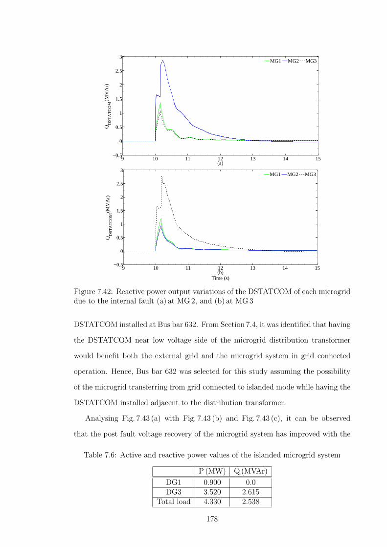
9 10 11 12 13 14 15−0.5

0

0.5

1

1.5

2

2.5

3

QD

ST

AT

CO

M (M

VA

r)

(a)

MG1 MG2 MG3

9 10 11 12 13 14 15−0.5

0

0.5

1

1.5

2

2.5

3

QD

ST

AT

CO

M (M

VA

r)

(b)Time (s)

MG1 MG2 MG3

Figure 7.42: Reactive power output variations of the DSTATCOM of each microgriddue to the internal fault (a) at MG 2, and (b) at MG 3

DSTATCOM installed at Bus bar 632. From Section 7.4, it was identified that having

the DSTATCOM near low voltage side of the microgrid distribution transformer

would benefit both the external grid and the microgrid system in grid connected

operation. Hence, Bus bar 632 was selected for this study assuming the possibility

of the microgrid transferring from grid connected to islanded mode while having the

DSTATCOM installed adjacent to the distribution transformer.

Analysing Fig. 7.43 (a) with Fig. 7.43 (b) and Fig. 7.43 (c), it can be observed

that the post fault voltage recovery of the microgrid system has improved with the

Table 7.6: Active and reactive power values of the islanded microgrid system

P (MW) Q (MVAr)

DG1 0.900 0.0DG3 3.520 2.615

Total load 4.330 2.538

178

9 9.5 10 10.5 11 11.5 120

0.2

0.4

0.6

0.8

1

1.2

1.4

X: 10.16Y: 0.3604

Vol

tage

(pu

)

(a)

632 634 645 646 675

9 9.5 10 10.5 11 11.5 120

0.2

0.4

0.6

0.8

1

1.2

1.4

X: 10.16Y: 0.3614

Vol

tage

(pu

)

(b)

632 634 645 646 675

9 9.5 10 10.5 11 11.5 120

0.5

1

1.5

X: 10.16Y: 0.3629

Vol

tage

(pu

)

(c)Time (s)

632 634 645 646 675

Figure 7.43: Voltage variations due to the internal fault (a) without DSTATCOM,(b) with DSTATCOM at DG1 terminal, (c) with DSTATCOM at Bus bar 632 duringislanded mode

DSTATCOM operation. Fig. 7.44 presents a comparison of the voltage at Bus bar

634 with and without DSTATCOM operation. Reactive power variations and reac-

tive current contributions from the DSTATCOM into the microgrid are presented

179

1-

1\ I '

I! ~,

i I I

_____ ______ ;

---- ~ - ----

w ~--~----_L-~--~----~----~--~

' '

----------------- .. -----------------------------

L] p

( ----------------------------------------------

9 9.5 10 10.5 11 11.5 120

0.2

0.4

0.6

0.8

1

1.2

1.4

Vol

tage

(pu

)

Time (s)

Without DSTATCOM At DG1 Terminal At Bus−633

Figure 7.44: Voltage variations due to the internal fault at Bus bar 634 duringislanded mode

in Fig. 7.45 and Fig. 7.46 respectively. On both occations, DSTATCOM supply the

full reactive power support after fault clearance.

9 10 11 12 13 14 15 16−0.5

0

0.5

1

1.5

QD

ST

AT

CO

M(MV

Ar)

Time (s)

At DG1 Terminal At Bus−632

Figure 7.45: Reactive power variations of the DSTATCOMs due to the fault at Busbar 645 during islanded mode

7.6.2 Multi-Microgrid System

In this section, operation of a DSTATCOM in a multi-microgrid system which is

islanded from the external grid is analysed. The multi-microgrid system illustrated

in Fig. 7.36 is used for the analysis without the external grid connection. Operating

conditions of the DGs of the microgrids and the loading conditions are presented

in Table. 7.7, where MG 1 operated in region R3, MG 2 and MG 3 operate in region

180

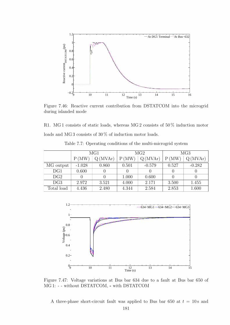
9 10 11 12 13 14 15 16−0.2

0

0.2

0.4

0.6

0.8

1

1.2

Rea

ctiv

e cu

rren

tD

ST

AT

CO

M (pu

)

Time (s)

At DG1 Terminal At Bus−632

Figure 7.46: Reactive current contribution from DSTATCOM into the microgridduring islanded mode

R1. MG 1 consists of static loads, whereas MG 2 consists of 50 % induction motor

loads and MG 3 consists of 30 % of induction motor loads.

Table 7.7: Operating conditions of the multi-microgrid system

MG1 MG2 MG3P (MW) Q (MVAr) P (MW) Q (MVAr) P (MW) Q (MVAr)

MG output -1.028 0.860 0.501 -0.579 0.527 -0.282DG1 0.600 0 0 0 0 0DG2 0 0 1.000 0.600 0 0DG3 2.972 3.521 4.000 2.171 3.500 1.455

Total load 4.436 2.480 4.344 2.584 2.853 1.600

9 10 11 12 13 14 150

0.2

0.4

0.6

0.8

1

1.2

Vol

tage

(pu

)

Time (s)

634−MG1 634−MG2 634−MG3

Figure 7.47: Voltage variations at Bus bar 634 due to a fault at Bus bar 650 ofMG 1: - - without DSTATCOM, - with DSTATCOM

A three-phase short-circuit fault was applied to Bus bar 650 at t = 10 s and

181

~~::- ~:: .... ~:::::::::::: •• :::;; ••.•• :;;-;-;; .••.• =.. . . ............. ...........--~ ,j?

9 10 11 12 13 14 15−0.5

0

0.5

1

1.5

2

2.5

Rea

ctiv

e cu

rren

t (pu

)

Time (s)

MG1 MG2 MG3

Figure 7.48: Reactive current variations through the distribution transformers ofthe microgrids due to the fault at Bus bar 650 of MG 1: - - without DSTATCOM,- with DSTATCOM

cleared after 160 ms. DSTATCOMs were considered to be connected on the low

voltage side of the microgrid distribution transformer in MG 1 and MG 2 each having

a 3 MVA rated capacity. Fig. 7.47 illustrates the voltage variations of Bus bar 643 of

each microgrid system due to the fault. It can be observed that the post fault voltage

recovery has improved with the presence of the DSTATCOMs in the multi-microgrid

system. Furthermore, reactive current contribution from each microgrid into the

fault has increased with the DSTATCOM operation as illustrated in Fig. 7.48.

For further analysis, another three-phase short-circuit fault was applied at the

terminal of an induction motor load in MG 2 (connected to Bus bar 652 in MG 2) at

t = 10 s and cleared after 160 ms. Fig. 7.49 (a) illustrates the voltage variations of the

bus bars at the high voltage side of the distribution transformer in each microgrid.

Fig. 7.49 (b) presents voltage variations of Bus bar 652 of each microgrid system due

to the fault. From both figures, it can be identified that the DSTATCOM operation

has improved the voltage profile of the microgrids. Fig. 7.50 illustrates the reactive

current variations through the distribution transformers of the microgrids due to a

fault at Bus bar 652 in MG 2. As a result of the DSTATCOM operation, reactive

current absorbed by MG 2 due to the internal fault has decreased, and reactive

current output from MG 1 has increased. Operation of DSTATCOMs in MG 1 and

182

. . \'

9 10 11 12 13 14 150.5

0.6

0.7

0.8

0.9

1

Vol

tage

(pu

)

(a)

650−MG1 650−MG2 650−MG3

9 10 11 12 13 14 150

0.2

0.4

0.6

0.8

1

Vol

tage

(pu

)

(b)Time (s)

652−MG1 652−MG2 652−MG3

Figure 7.49: Voltage variations of (a) Bus bar 650, and (b) Bus bar 652 in eachmicrogrid due to the fault at Bus bar 652 of MG 2: - - without DSTATCOM, - withDSTATCOM

MG 2 has reduced the reactive current flowing out of MG 3 which does not have a

DSTATCOM. Hence, by examining all the results, it is clear that the operation of

DSTATCOM in islanded microgrid systems improve the system bahaviour caused

by faults.

7.7 Impact of Induction Motor Loads and DSTATCOM

In this section, a case study was carried out to investigate grid connected microgrid

behaviour with DSTATCOM and induction motor loads. The microgrid system

described in Section 7.4.1 was considered for the study and DG3 was assumed to be

disconnected resulting the microgrid to operate in region R2. Steady state active

183

" " ~

____ .. ...... --------__ ......... ------ .. ---------

_ •• ~---:-:::-:::::;;:::::-:::::-: ~=: •• ~ ... "..... . ..

............

9 10 11 12 13 14 15−0.8

−0.6

−0.4

−0.2

0

0.2

0.4

0.6

Rea

ctiv

e cu

rren

t (pu

)

Time (s)

MG1 MG2 MG3

Figure 7.50: Reactive current variations through the distribution transformers ofthe microgrids due to the fault at Bus bar 652 of MG 2: - - without DSTATCOM,- with DSTATCOM

and reactive power levels considered for this case study are presented in Table 7.8

and a 3 MVA DSTATCOM is connected at Bus bar 632.

Table 7.8: Active and reactive power values in the microgrid

P (MW) Q (MVAr)

DG1 0.500 0.0DG2 0.900 0.0

Total load 2.818 1.582

Fig. 7.51 illustrates the voltage variation of bus bars in the microgrid due to a

three-phase short-circuit fault applied at Bus bar 650 for 160 ms. Fig. 7.51 (a) corre-

sponds to the scenario with only static load models, whereas in Fig. 7.51 (b), 40 % of

the total microgrid load was replaced with induction motor models. When loads are

represented by static loads, the post fault voltage of the microgrid recovered quickly

to the pre-fault value with the DSTATCOM. However, even with the DSTATCOM,

the voltage has decreased during the fault with induction motor load models, due

to induction motor reactive power requirement. Furthermore, post-fault voltage has

taken more time to reach the pre-fault voltage profile of the microgrid with induction

motor models.

Similarly, a three-phase short-circuit fault was applied inside the microgrid at

Bus bar 652 at t = 10 s, and cleared after 150 ms. Fig. 7.52 (a) and Fig. 7.52 (b)

184

... ~- .. -- _ .. -.. ----- _ ..... --------

~I ----+--------+--1

9 9.5 10 10.5 11 11.5 120

0.5

1

1.5

Vol

tage

(pu

)

(a)

650 632 646 634 652

9 9.5 10 10.5 11 11.5 120

0.5

1

1.5

Vol

tage

(pu

)

(b)Time (s)

650 632 646 634 652

Figure 7.51: Voltage variations of bus bars due to the fault at Bus bar 650 withDSTATCOM for (a) only static loads, and (b) with induction motor loads

illustrate the voltage profile with only static loads and with 40 % induction motor

load respectively. Due to the reactive power requirement of the induction motor

loads, post-fault voltage recovery of the microgrid can be seen to be slow compared

to the microgrid with only static loads even in the presence of DSTATCOM.

Fig. 7.53 (a) and Fig. 7.53 (b) illustrate the reactive power output of the DSTAT-

COM at Bus bar 632 for the faults at Bus bar 650 and Bus bar 652 respectively. By

examining both figures, it can be observed that the DSTATCOM has supplied more

reactive power to the system after fault clearance when the microgrid consisted of

induction load models. During the fault, amount of reactive power supplied by the

DSTATCOM depends on the DSTATCOM terminal voltage.

185

rf ------------- ----- --- ________________________________ _

rN -----------------------------------------------

9 9.5 10 10.5 11 11.5 120

0.5

1

1.5

Vol

tage

(pu

)

(a)

650 632 646 634 652

9 9.5 10 10.5 11 11.5 120

0.2

0.4

0.6

0.8

1

Vol

tage

(pu

)

(b)Time (s)

650 632 646 634 652

Figure 7.52: Voltage variations at bus bars due to the fault at Bus bar 652 withDSTATCOM for (a) only static loads, and (b) with induction motor loads

7.8 Summary

This chapter presented detailed case studies carried out to investigate DSTATCOM

operation in microgrids and the ability to support both microgrid and the external

grid during faults. Microgrids operating in four different regions (four quadrants)

were subjected to external and internal faults with and without DSTATCOM and

the microgrid behaviour was analysed. The reactive power contribution from the

microgrid increased during faults due to the DSTATCOM operation and post fault

transients have reduced.

Impact of the DSTATCOM location in the microgrid was also analysed by in-

stalling the DSTATCOM on the low voltage side of the microgrid distribution trans-

former, at DG terminals and at the bus bar with minimum reactive power margin

186

9 9.5 10 10.5 11 11.5 12−1

−0.5

0

0.5

1

1.5

2

2.5

3

QD

ST

AT

CO

M (M

VA

r)

(a)

Static load models With induction motor models

9 9.5 10 10.5 11 11.5 12−0.5

0

0.5

1

1.5

2

2.5

3

QD

ST

AT

CO

M (M

VA

r)

(b)Time

Static load models Induction motor models

Figure 7.53: Reactive power output of the DSTATCOM for the fault at (a) Bus bar650, and (b) Bus bar 652

of the microgrid. Variations of the microgrid system parameters during the fault

and after fault clearance were analysed to identify the most appropriate location of

DfSTATCOM.

Furthermore, DSTATCOMs were installed in a multi-microgrid system and the

system was subjected to different faults. Response of DSTATCOMs in single and

multi-microgrid systems during islanded operation were also analysed. Installing

DSTATCOM on low voltage side of the microgrid distribution transformer provides

better performance in both grid connected and islanded modes. During grid con-

nected mode, DSTATCOM will provide better voltage and reactive power support

to the external grid as well as improve microgrid voltage profile. Having the DSTAT-

COM on the low voltage side of the microgrid distribution transformer will be an

advantage and will improve the microgrid overall voltage profile, if the microgrid

187

\ -,

' ' ' ' ' ' ' ' ' ' ' ' ,, ,, ,, ,, ,,

~~-L~~-~~_j__, ti

'' '' \J

' . ' ' . . . .

'

~__j____,_~_,____[_ '

. . . ' '

'

-.. ..... .. ..... -........... __ ~~--~

transfer from grid connected to islanded mode of operation. DSTATCOM operation

would reduce the reactive power demand from the external grid arising during faults

from microgrids having induction motor loads.

Similar to a DG with reactive power capability, DSTATCOM can be used as a

mechanism to provide reactive power support from microgrid to the external grid

during low voltage ride through events. However, depending on the capacity of the

microgrid, required capacity of the DSTATCOM would change. Thus, it is important

to carry out a financial analysis when planning to install DSTATCOM in microgrids.

Furthermore, future work would also involve in analysing the placement and sizing

of DSTATCOM in microgrid environment under different operating conditions.

188

Chapter 8

Conclusions and Future Work

8.1 Summary and Conclusions

Increasing penetration level of DERs have transformed distribution networks from

passive to active networks and introduced the concept of microgrids. Through a

comprehensive literature review carried out in this thesis, some key issues and re-

search gaps were identified related to microgrid modelling and operation. While

embarking on the research gaps identified on microgrids, this thesis has examined

a number of issues related to the modelling of microgrids, and has investigated

different aspects of their operation.

In the first phase of this thesis, the dynamic characteristics associated with mi-

crogrids comprising inverter and non-inverter interfaced DERs were investigated.

Preliminary studies were carried out on a simulation microgrid model developed

comprising a PV system, a DFIG based wind power plant, a mini hydro power

plant, and loads. The importance of understanding the dynamic behaviour of mi-

crogrids was highlighted through a comparative analysis carried out on the hybrid

microgrid. This study revealed that the dynamic characteristics of the microgrid

are significantly influenced by the individual characteristics of DERs and their con-

trol systems. The study examined the influence of the variations in active power

dispatch levels and generator relative sizing on the dynamic characteristics of the

microgrid.

189

It was clearly evident that the DERs with a directly coupled rotor to the net-

work have a signiffcant influence on the post fault oscillations in the microgrid as

the inertial response of inverter interfaced DER is either unavailable (e.g. PV sys-

tem) or decoupled from the network (e.g. DFIG). Microgrids with smaller system

rotational inertia have a larger frequency deviation for a given mismatch between

load and power generation. Depending on the speed, accuracy and artificial damp-

ing provided by the controllers, the inverter interfaced DERs would also have a

substantial impact on the microgrid stability. The fast controllers would allow the

inverter interfaced DERs to respond to disturbances quickly and reach steady-state

after fault clearance. Furthermore, it has been shown that the ROCOF increased

with the increasing penetration of inverter-interfaced DERs. It has been noted that

during grid connected mode, features of the external grid also have an impact on

the microgrid behaviour. It was highlighted that the external grid SCC plays an

important role in maintaining an acceptable microgrid voltage profile. Moreover,

grid connected microgrids were able to recover faster due to faults when compared

to islanded microgrids.

Distribution networks can no longer be represented merely by a static load at

the PCC. In particular, dynamics of microgrids during grid connected mode must be

taken into account in order to accurately characterise the stability of the network.

Unlike traditional SGs and their auxiliary components, effects of grid connected

microgrid dynamics on large power systems have yet to be completely characterised.

Thus, the second phase of this thesis was focused on aggregated modelling of grid

connected microgrids comprising both inverter and non-inverter interfaced DERs.

For stability analysis, the common practice is to separate the power system into

a study area of interest and external areas. In general, the study area is represented

in a detailed manner while external areas are represented by dynamic equivalents.

Thus, the microgrids in the external areas can be represented by linearised single

dynamic devices while retaining the important dynamics. It was identified that the

basic modal method had not been previously applied to grid connected microgrids

190

comprising both inverter and non-inverter interfaced DERs as a model equivalencing

methodology. Thus, the thesis investigated the applicability of modal analysis as

a tool for model equivalencing of grid connected microgrids having inverter and

non-inverter interfaced DERs.

Detailed models of an inverter interfaced DERs with power controllers, non-

inverter interfaced DERs with governor and excitation controllers, induction motor

load and network were developed as a basis for the studies. A new index was defined

for identifying the dominant modes which needed to be retained in the reduced or-

der equivalent of the microgrid. Model equivalencing methodology was applied to

a five-bus microgrid system comprising two DERs and two types of loads. Several

case studies were carried out under different operating conditions of the microgrid

system. Furthermore, scalability of the proposed microgrid model equivalencing

approach was demonstrated using a larger microgrid model based on the IEEE-13

node distribution test feeder and a multi-microgrid system. It was observed that

the responses of the microgrid system states and the microgrid current outputs ob-

tained from the full order model and reduced order equivalent model were in good

agreement. Thus, the proposed dynamic model equivalent of the grid connected

microgrid based on basic modal method has captured the important dynamics of

the full order microgrid systems. However, a limitation of the modal method exists

due to the linearisation of the microgrid system. Thus, this dynamic equivalencing

method can be used for system studies when grid connected microgrids are not di-

rectly subjected to large internal disturbances or when the investigated disturbances

are not placed too close to the boundary of the microgrid equivalent model.

The process of deriving the dynamic equivalent models of grid connected mi-

crogrids can be automated in power system simulation software packages and can

be replaced with a current source having the nominal output current with nominal

voltage at the microgrid PCC. However, one advantage of this method over the other

model training methods is that, once a dynamic equivalent has been obtained for

a grid connected microgrid, numerous faults can be analysed in the study system

191

using the same equivalent. However, as above, the faults cannot be placed too close

to the boundary of the microgrid equivalent model.

Unlike in a single generator unit with its own machine limitations, active and

reactive power transfer limits of a grid connected microgrid depend on many factors


distribution line capacities. By conducting a thorough literature survey, it was

identified that no research knowledge existed related to identifying power transfer

capability limits of grid connected microgrids. Absence of such knowledge was the

primary drive for developing a systematic approach for deriving a capability diagram

for a grid connected microgrid in the third phase of this thesis.

In order to derive the capability diagram, a non-linear optimisation model was

developed considering individual machine limitations, local load demands, distribu-

tion line capacities, transformer capacities and network voltage limitations. Using

the optimisation model, simplified capability diagrams were obtained for two grid

connected microgrid systems. Both capability diagrams represented the active and

reactive power exchange capability of the microgrids at the PCC. From the results,

it was identified that considering simplified DG machine capability limitations would

yield inaccurate microgrid power exchange capability with the external grid. Hence,

incorporation of realistic DG machine limitations into the optimisation model is

essential in order to derive an accurate microgrid active and reactive power capa-

bility diagram. Impact of different voltage regulation systems was analysed and it

was noted that an increase in the range of acceptable voltage variation at the buses

within the microgrid is favourable for power export from the microgrid. Further-

more, for the same local loading conditions, power import and export capability

of the microgrid can be increased by allowing the voltage at the PCC to be var-

ied within an acceptable limit, rather than fixing at a particular voltage level. The

shape and size of the capability diagram vary with microgrid generation and loading

conditions, as different constraints/limits are met in the optimisation model at each

power flow. Impact of individual distributed generator outages on the capability

192

diagram was also demonstrated using two microgrid systems.

It was noted that charging and discharging pattern of individual PHEVs in mi-

crogrids has a negligible impact on the capability diagram as their size is comparably

small compared to the DERs. However, the effect of charging and discharging of

a fleet of PHEVs can be represented as simple loads or generators in the optimi-

sation model. Applicability of capability diagrams as a tool in the energy market

operation was also described. Electricity costs corresponding to all the points of the

microgrid capability diagram were derived based on both active and reactive power

markets in separate study cases. It was demonstrated that such capability diagrams

with economic aspects can be utilisded by the MCC or DNSPs to harness maximum

possible power from the microgrids.

In the fourth phase, this thesis investigated the LVRT capability of grid con-

nected microgrids as an ancillary service provider to the utility grid. Two approaches

were followed to investigate the LVRT capability of a microgrid as a single entity. In

the first approach, dynamic voltage support at the microgrid PCC was improved by

using a DSTATCOM at the low voltage side of the distribution transformer of the

microgrid. Faults were created at the external grid and the active and reactive power

responses from the microgrid PCC were examined. It was observed that irrespective

of the active and reactive power flow direction at the microgrid PCC, the microgrid

with the DSTATCOM installed provided additional reactive power during and after

the fault clearance. Furthermore, the CCT of the microgrid has improved with the

operation of DSTATCOM. The collective effect of the reactive power capabilities of

the distributed generators in the microgrid was used to provide voltage and reactive

power support to the external grid in the second approach. Instead of the inbuilt

LVRT capability of DGs, DSTATCOMs were installed at the terminal of the DGs.

Improved DG LVRT capability may also achieve similar results.

Furthermore, DSTATCOMs were installed in a multi-microgrid system and the

system was subjected to different faults. Response of DSTATCOMs single and

multi-microgrid systems in islanded operation were also analysed. It was noted

193

that by installing a DSTATCOM at low voltage side of the microgrid distribution

transformer would provide better performance in both grid connected and islanded

modes. During grid connected mode, DSTATCOM would provide better voltage

and reactive power support to the external grid as well as improve microgrid voltage

profile. Having the DSTATCOM on the low voltage side of the microgrid distribution

transformer would improve microgrid overall voltage profile if the microgrid transfer

from grid connected to islanded mode of operation. The DSTATCOM would reduce

the reactive power demand from the external grid arising during faults in microgrids

with induction motor loads. Similar to a DG with LVRT capability, DSTATCOM

can be used as a mechanism to provide reactive power support from microgrid to the

external grid during faults. However, depending on the capacity of the microgrid,

required capacity of the DSTATCOM would change. Thus, it is important to carry

out a financial study when planning to install DSTATCOMs within microgrids.

From a careful analysis, it was concluded that having the DSTATCOM installed

on the low voltage side of the microgrid distribution transformer has better impact

on all the buses of the microgrid compared to the DSTATCOM installed at other

locations studied. When the DSTATCOM is not installed on the low voltage side

of the microgrid distribution transformer, the microgrid is unable to utilise the

maximum capability of the DSTATCOM to provide support to the external grid.

During the post fault transients, reactive power absorption from the microgrid is

minimum when the DSTATCOM is installed on the low voltage side of the microgrid

distribution transformer.

8.2 Recommendations for Future Work

In the future, when microgrids become more commonplace with higher penetration

of DERs, the stability and security of the utility grid will be affected significantly.

Thus, microgrids need to be designed properly to take care of their dynamic impact

on the utility grid such that the overall stability and reliability of the whole system

is maintained or significantly improved.

194

As the dynamic response of inverter interfaced DERs depends on the applied

control starategy, future work would be required to study the microgrid behaviour

incorporating various control algorithms in different types of DERs. Furthermore,

single phase elements (e.g. PV systems and loads) need to be considered with three-

phase elements in microgrids, and should conduct time domain simulations using

DIgSILENT PowerFactory in order to study the dynamics.

The grid connected microgrid model equivalencing methodology presented in

this thesis can be applied for microgrids with any operating mode with any type of

control algorithms as long as the control algorithms do not change for the considered

time frame. For the time frame of interest, dynamics of the dc side of the inverter

interfaced DERs were considered negligible. Once the dc side dynamics are included

in the state-space model using ODEs, any change in dc side dynamics would result

in a change in the initial values of the microgrid model. Future work will be carried

out to investigate the impact of the variation of dc side dynamics on the full order

microgrid model and the reduced order microgrid model. Furthermore, future work

will include experimental verification of the microgrid equivalencing methodology

proposed in this thesis including both inverter and non-inverter interfaced DERs

and different types of loads. Depending on the capabilities and requirements of

different simulation packages, dynamic equivalents of microgrids can be implemented

as controlled current sources with nominal output current from the microgrid as

suggested in Chapter 5 of this thesis. This would allow the grid connected microgrid

systems to be implemented in simulation packages with reduced size and complexity.

The methodology of deriving capability diagrams of grid connected microgrid

systems as presented in Chapter 6 can be derived in real time, provided proper

communication media exists between the generators, load centres and the MCC.

Furthermore, the proposed methodology and the mathematical model can incor-

porate other optimisation algorithms for developing capability diagrams. Thus, a

comparative analysis can be carried out using different optimisations algorithms on

microgrid capability diagrams.

195

Operation of microgrids in the energy market can be more complex when de-

mand side bidding is considered. The MCC has to optimise the operation of the

microgrid by considering the bids from both DGs and loads. If consumers are willing

to shed loads, the MCC will be required to pay a curtailment fee which will con-

tribute to the microgrid operating costs. As the work in this thesis focuses on the

grid connected mode of operation of microgrids, future work will include business

models for microgrids different to the two business models presented in Chapter 6.

A more detailed analysis with different market models and the impact on microgrid

power import and export capability diagram is identified as future work arising from

Chapter 6.

This thesis only investigates the technical assessment of DSTATCOM for mi-

crogrids and its advantage for grid connected and islanded modes of operation. As

future work, coordination of other voltage control devices operating within the dis-

tribution system such as capacitor banks, transformer tapping etc. will be taken

into consideration. With LVRT capability, the DSTATCOM can be used as a mech-

anism to provide reactive power support from microgrid to the external grid during

faults. However, depending on the capacity of the microgrid, required capacity of

the DSTATCOM would change. Thus, it is important to carry out a financial study

when planning to install the DSTATCOM in microgrids. Future work would also

be required for analysing the placement and sizing of the DSTATCOM in microgrid

environment under different operating conditions. Furthermore, a more detailed

economic analysis will be carried out in order to determine if it is cheaper for hav-

ing distributed LVRT performance expectation from all microgrid components or a

simpler DSTATCOM solutionfor the entire microgrid.

196

References

[1] G. Venkataramanan and C. Marnay. A Larger Role for Microgrids. Power

and Energy Magazine, IEEE, 6(3):78–82, May 2008.

[2] J. A. Peas Lopes, N. Hatziargyriou, J. Mutale, P. Djapic, and N. Jenkins.

Integrating Distributed Generation into Electric Power Systems: A Review

of Drivers, Challenges and Opportunities. Electric Power Systems Research,

77(9):1189 – 1203, 2007.

[3] F. Katiraei, R. Iravani, N. Hatziargyriou, and A. Dimeas. Microgrids Man-

agement. Power and Energy Magazine, IEEE, 6(3):54–65, May 2008.

[4] B. Kroposki, R. Lasseter, T. Ise, S. Morozumi, S. Papatlianassiou, and

N. Hatziargyriou. Making Microgrids Work. Power and Energy Magazine,

IEEE, 6(3):40–53, May 2008.

[5] N. W. A. Lidula and A. D. Rajapakse. Microgrids Research: A Review of Ex-

perimental Microgrids and Test Systems. Renewable and Sustainable Energy

Reviews, 15(1):186 – 202, 2011.

[6] N. Hatziargyriou. Microgrids:Architectures and Control. Wiley-IEEE Press,

2014.

[7] R. H. Lasseter, J. H. Eto, B. Schenkman, J. Stevens, H. Vollkommer, D. Klapp,

E. Linton, H. Hurtado, and J. Roy. CERTS Microgrid Laboratory Test Bed.

IEEE Trans. on Power Delivery, 26(1):325–332, Jan. 2011.

[8] T. Ackermann, G. Andersson, and L. Sder. Distributed Generation: A Defi-

nition. Electric Power Systems Research, 57(3):195 – 204, 2001.

[9] J. Driesen and F. Katiraei. Design for Distributed Energy Resources. Power

and Energy Magazine, IEEE, 6(3):30–40, May 2008.

[10] S. Chowdhury, S. P. Chowdhury, and P. Crossley. Microgrids and Active

Distribution Networks. The Institution of Engineering and Technology, 2009.

197

[11] T. L. Vandoorn, J. C. Vasquez, J. De Kooning, J. M. Guerrero, and L. Van-

develde. Microgrids: Hierarchical Control and an Overview of the Control

and Reserve Management Strategies. Industrial Electronics Magazine, IEEE,

7(4):42–55, Dec. 2013.

[12] R. Masiello and S. Venkata. Microgrids: There May Be One in Your Future.

Power and Energy Magazine, IEEE, 11(4):14–93, July 2013.

[13] N. Hatziargyriou, H. Asano, R. Iravani, and C. Marnay. Microgrids. Power

and Energy Magazine, IEEE, 5(4):78–94, July 2007.

[14] C. Abbey, D. Cornforth, N. Hatziargyriou, K. Hirose, A. Kwasinski, E. Kyr-

iakides, G. Platt, L. Reyes, and S. Suryanarayanan. Powering Through the

Storm: Microgrids Operation for More Efficient Disaster Recovery. Power and

Energy Magazine, IEEE, 12(3):67–76, May 2014.

[15] L. Schmitt, J. Kumar, D. Sun, S. Kayal, and S. S. M. Venkata. Ecocity Upon

a Hill: Microgrids and the Future of the European City. Power and Energy

Magazine, IEEE, 11(4):59–70, July 2013.

[16] T. Tanabe, Y. Ueda, T. Funabashi, S. Numata, K. Morino, and E. Shimoda.

An Active Network Control Method using Distributed Energy Resources in

Microgrids. In Proc. Power Electronics and Motion Control, pages 2478–2480,

Sept. 2008.

[17] C. K. Sao and P. W. Lehn. Control and Power Management of Converter Fed

Microgrids. IEEE Trans. on Power Systems, 23(3):1088–1098, Aug. 2008.

[18] A. L. Dimeas and N. D. Hatziargyriou. Operation of a Multiagent System for

Microgrid Control. IEEE Trans. on Power Systems, 20(3):1447–1455, Aug.

2005.

[19] J. C. Matas J. de Vicua L. G. Guerrero, J. M. Vasquez and Castilla M. Hi-

erarchical Control of Droop - Controlled AC and DC Microgrids-A General

198

Approach Toward Standardization. IEEE Trans. on Industrial Electronics, 58

(1):158–172, 2011.

[20] D. T. Ton, W. M. Wang, and W. T. P. Wang. Smart Grid R & D by the U.S.

Department of Energy to Optimize Distribution Grid Operations. In Power

and Energy Society General Meeting, IEEE, pages 1–5, July 2011.

[21] N. Hatziargyriou, N. Jenkins, and G. Strbac. Microgrids-Large Scale Integra-

tion of Microgeneration to Low Voltage Grids. In Proc. CIGRE, Aug. 2006.

[22] N. Hatziargyriou. Advanced Architectures and Control Concepts for More

Microgrids, http://www.microgrids.eu/documents/esr.pdf, Feb. 2014.

[23] T. Loix. The First Microgrid in the Netherland: Bronsbergen, Feb. 2009.

[24] B. Buchholz, N. Hatziargyriou, I. Furones, and U. Schluecking. Lessons

Learned: European Pilot Installations for Distributed Generation - An

Overview by the IRED Cluster. In Proc. CIGRE, Aug 2006.

[25] M. Barnes, J. Kondoh, H. Asano, J. Oyarzabal, G. Ventakaramanan, R. Las-

seter, N. Hatziargyriou, and T. Green. Real-World Microgrids - An Overview.

In Proc. IEEE System of Systems Engineering, pages 1–8, Apr. 2007.

[26] S. Morozumi, H. Nakama, and N. Inoue. Demonstration Projects for Grid-

Connection Issues in Japan. Elektrotechnik & Informationstechnik, 125

(3):426–431, Dec. 2008.

[27] K. Hirose, T. Takeda, and S. Muroyama. Study on Field Demonstration of

Multiple Power Quality Levels System in Sendai. In Proc. Telecommunications

Energy Conf., Sept 2006.

[28] C. Marnay and N. Zhou. Status of Overseas Microgrid Programs: Microgrid

Research Activities in the U.S. (English Version), Feb. 2008.

199

[29] E. Alegria, T. Brown, E. Minear, and R. H. Lasseter. CERTS Microgrid

Demonstration with Large-Scale Energy Storage and Renewable Generation.

IEEE Trans. on Smart Grid, 5(2):937–943, March 2014.

[30] R. Majumder. Some Aspects of Stability in Microgrids. IEEE Trans. on Power

Systems, 28(3):3243–3252, Aug. 2013.

[31] R. Kamel, A. Chaouachi, and K. Nagasaka. Detailed Analysis of Micro-Grid

Stability during Islanding Mode under Different Load Conditions. Engineering,

3(5):508–516, 2011.

[32] D. P. Ariyasinghe and D. M. Vilathgamuwa. Stability Analysis of Microgrids

with Constant Power Loads. In Proc. Sustainable Energy Technologies, pages

279–284, Nov. 2008.

[33] D. M. Vilathgamuwa, X. N. Zhang, S. D. G. Jayasinghe, B. S. Bhangu, C. J.

Gajanayake, and K. J. Tseng. Virtual Resistance Based Active Damping

Solution for Constant Power Instability in AC Microgrids. In Proc. Annual

Conf. on IEEE Industrial Electronics Society, pages 3646–3651, Nov. 2011.

[34] H. Karimi, H. Nikkhajoei, and R. Iravani. Control of an Electronically-Coupled

Distributed Resource Unit Subsequent to an Islanding Event. IEEE Trans.

on Power Delivery, 23(1):493–501, Jan. 2008.

[35] F. Katiraei, M. R. Iravani, and P. W. Lehn. Micro-grid Autonomous Operation

During and Subsequent to Islanding Process. IEEE Trans. on Power Delivery,

20(1):248–257, Jan. 2005.

[36] M. Shahabi, M. R. Haghifam, M. Mohamadian, and S. A. Nabavi-Niaki. Mi-

crogrid Dynamic Performance Improvement using a Doubly Fed Induction

Wind Generator. IEEE Trans. on Energy Conversion, 24(1):137–145, March

2009.

200

[37] Z. Miao, A. Domijan, and L. Fan. Investigation of Microgrids with Both

Inverter Interfaced and Direct AC-Connected Distributed Energy Resources.

IEEE Trans. on Power Delivery, 26(3):1634–1642, July 2011.

[38] M. Dewadasa, A. Ghosh, and G. Ledwich. Dynamic Response of Distributed

Generators in a Hybrid Microgrid. In Power and Energy Society General

Meeting, IEEE, July 2011.

[39] N. Pogaku, M. Prodanovic, and T. C. Green. Modeling, Analysis and Testing

of Autonomous Operation of an Inverter-Based Microgrid. IEEE Trans. on

Power Electronics, 22(2):613–625, March 2007.

[40] D. J. Lee and Wang. Li. Small-Signal Stability Analysis of an Autonomous

Hybrid Renewable Energy Power Generation/Energy Storage System Part I:

Time-Domain Simulations. IEEE Trans. on Energy Conversion, 23(1):311–

320, March 2008.

[41] F. Katiraei and M. R. Iravani. Power Management Strategies for a Microgrid

with Multiple Distributed Generation Units. IEEE Trans. on Power Systems,

21(4):1821–1831, Nov. 2006.

[42] R. Majumder, A. Ghosh, G. Ledwich, and F. Zare. Control of Parallel Con-

verters for Load Sharing with Seamless Transfer between Grid Connected and

Islanded Modes. In Power and Energy Society General Meeting, IEEE, July

2008.

[43] J. Machowski, A. Cichy, F. Gubina, and P. Omahen. External Subsystem

Equivalent Model for Steady-State and Dynamic Security Assessment. IEEE

Trans. on Power Systems, 3(4):1456–1463, Nov. 1988.

[44] E. M. De Oliveira, Sebastio and J. F. De Queiroz. Modal Dynamic Equiva-

lent for Electric Power Systems. I. Theory. IEEE Trans. on Power Systems,

3(4):1723–1730, Nov. 1988.

201

[45] J. M. Undrill, J. A. Casazza, E. M. Gulachenski, and L. K. Kirchrnayer.

Electromechanical Equivalent for use in Power System Stability Studies. IEEE

Trans. on Power Apparatus and Systems, PAS-90(5):2060–2071, Sept. 1971.

[46] J. M. Undrill and A. E. Turner. Construction of Power System Electrome-

chanical Equivalents by Modal Analysis. IEEE Trans. on Power Apparatus

and Systems, PAS-90(5):2049–2059, Sept. 1971.

[47] E. Davison. A Method for Simplifying Linear Dynamic Ssystems. IEEE Trans.

on Autom. Control, 11(1):93–101, Jan. 1966.

[48] H. Altalib and P. Krause. Dynamic Equivalents by Combination of Reduced

Order Models of System Components. IEEE Trans. on Power App. Syst,

95:1535–1544, Sept. 1976.

[49] A. Kuppurajulu and S. Elangovan. Simplified Power System Models for Dy-

namic Stability Studies. IEEE Trans. on Power Apparatus and Systems, PAS-

90(1):11–23, Jan. 1971.

[50] G. Perez-Arriaga, I. Verghese and F. Schweppe. Selective Modal Analysis with

Applications to Electric Power Systems, Part I: Heuristic Introduction,. IEEE

Trans. on Power App. Syst., PAS-101(9):3117–3125, Sept. 1982.

[51] I. S. F. Verghese and G.C. Perez-Arriaga. Selective Modal Analysis with Ap-

plications to Electric Power Systems, Part II: The Dynamic Stability Problem.

IEEE Trans. on Power App. Syst., PAS-101(9):3126– 3134, Sept. 1982.

[52] G. Ramaswamy, G. Verghese, L. Rouco, C. Vialas, and C. DeMarco. Syn-

chrony, Aggregation, and Multi-area Eigenanalysis. IEEE Trans. on Power

Systems, 12:1986–1993, Nov. 1995.

[53] G. Ramaswamy, C. Evrard, G. Verghese, O. Fillatre, and B. Lesieutre. Exten-

sions, Simplifications, and Tests of Synchronic Modal Equivalencing (SME).

IEEE Trans. on Power Systems, 12:896–905, May 1997.

202

[54] J. H. Chow, R. Galarza, P. Accari, and W. W. Price. Inertial and Slow Co-

herency Aggregation Algorithms for Power System Dynamic Model Reduction.

IEEE Trans. on Power Systems, 10(2):680–685, May 1995.

[55] A. Ischchenko, X. A. MyrzTang, and W. L. Kling. Dynamic Equivalencing

of Distribution Networks with Dispersed Generation. In Power Engineering

Society General Meeting, IEEE, 2006.

[56] A. Ishchenko, J. M. A. Myrzik, and W. L. Kling. Dynamic Equivalencing of

Distribution Networks with Dispersed Generation using Hankel Norm Approx-

imation. Generation, Transmission & Distribution, IET, 1:818–825, 2007.

[57] P. V. Kokotovic, R. E. Jr. O’Malley, and P. Sannuti. Singular Perturbations

and Order Reduction in Control Theory - An Overview. Automatica, 12(2):123

– 132, 1976.

[58] R. M. G. Castro and J. M. Ferreira De Jesus. A Wind Park Reduced-Order

Model using Singular Perturbations Theory. IEEE Trans. on Energy Conver-

sion, 11(4):735–741, Dec. 1996.

[59] S.K. Joo, C. C. Liu, L. E. Jones, and J.W. Choe. Coherency and Aggrega-

tion Techniques Incorporating Rotor and Voltage Dynamics. IEEE Trans. on

Power Systems, 19(2):1068–1075, May 2004.

[60] A. J. Germond and R. Podmore. Dynamic Aggregation of Generating Unit

Models. IEEE Trans. on Power Apparatus and Systems, PAS-97(4):1060–1069,

July 1978.

[61] R. Podmore. Identification of Coherent Generators for Dynamic Equivalents.

IEEE Trans. Power Apparatus and Systems,, PAS-97(4):1344–1354, July 1978.

[62] R. Nath, S. S. Lamba, and K. S. Prakasa Rao. Coherency Based System

Decomposition into Study and External Areas using Weak Coupling. IEEE

Trans. on Power Apparatus and Systems, PAS-104(6):1443–1449, June 1985.

203

[63] J. R. Winkelman, J. H. Chow, B. C. Bowler, B. Avramovic, and P. V. Koko-

tovic. An Analysis of Interarea Dynamics of Multi-Machine Systems. IEEE

Trans. on Power Apparatus and Systems, PAS-100(2):754–763, Feb. 1981.

[64] S. T. Y. lee and F. C. Schweppe. Distance Measures and Coherency Recogni-

tion for Transient Stability Equivalents. IEEE Trans. Power Appar. & Syst,

PAS-92:1550–1557, Sept/ Oct 1973.

[65] T. N. Nababhushana, K. T. Veeramanju, and Shivanna. Coherency Identifi-

cation using Growing Self Organizing Feature Maps [Power System Stability].

In Proc. Energy Management and Power Delivery Conf., pages 113–116 (1),

March 1998.

[66] Z. Shuqiang, C. Xianrong, P. Yunjiang, and H. Renmu. A Reduced Order

Method for Swing Mode Eigenvalue Calculating Based on Fuzzy Coherency

Recognition. In Proc. Power System Technology Conf., pages 1402–1405 (2),

Aug. 1998.

[67] M. H. Haque and A. H. M. A. Rahim. An Efficient Method of Identifying

Coherent Generators using Taylor Series Expansion. IEEE Trans. on Power

Systems, 3(3):1112–1118, Aug. 1988.

[68] L. Wang, M. Klein, S. Yirga, and P. Kundur. Dynamic Reduction of

Large Power Systems for Stability Studies. IEEE Trans. on Power Systems,

12(2):889–895, May 1997.

[69] M. L. Ourari, L. A. Dessaint, and Van-Que Do. Dynamic Equivalent Modeling

of Large Power Systems using Structure Preservation Technique. IEEE Trans.

on Power Systems, 21(3):1284–1295, Aug. 2006.

[70] R. Nath and S. S. Lamba. Development of Coherency-based Time-domain

Equivalent Model using Structure Constraints. Generation, Transmission and

Distribution, IEE, 133(4):165–175, May 1986.

204

[71] T. L. Le, Q. T. Tran, O. Devaux, O. Chilard, and R. Caire. Reduction and

Aggregation for Critical and Emergency Operation of Distribution Network in

Presence of Distributed Generators. In Proc. 20th IntN. Conf. and Exhibition

Electricity Distribution - Part 1, June 2009.

[72] V. Sankaranarayanan, M. Venugopal, S. Elangovan, and N. Dharma Rao. Co-

herency Identification and Equivalents for Transient Stability Studies. Electric

Power Systems Research, 6(1):51 – 60, 1983.

[73] S. Geeves. A Modal-Coherency Technique for Deriving Dynamic Equivalents.

IEEE Trans. on Power Systems, 3(1):44–51, Feb. 1988.

[74] H. Oh. Aggregation of Buses for a Network Reduction. IEEE Trans. on Power

Systems, 27(2):705–712, May 2012.

[75] J. Machowski, J. W. Bialek, and J. R. Bumby. POWER SYSTEM DYNAM-

ICS Stability and Control. John Wiley & Sons, Ltd., 2008.

[76] X. Feng, Z. Lubosny, and J.W. Bialek. Identification based Dynamic Equiva-

lencing. In Proc. IEEE Lausanne Power Tech., pages 267–272, July 2007.

[77] X. Feng, Z. Lubosny, and J. Bialek. Dynamic Equivalencing of Distribution

Network with High Penetration of Distributed Generation. In Proc. Int. Uni-

versities Power Engineering Conf., pages 467–471 (2), Sept. 2006.

[78] P. N. Papadopoulos, T. A. Papadopoulos, P. Crolla, A. J. Roscoe, G. K. Pa-

pagiannis, and G. M. Burt. Black-Box Dynamic Equivalent Model for Micro-

grids using Measurement Data. Generation, Transmission Distribution, IET,

8(5):851–861, May 2014.

[79] J. V. Milanovic and S. Mat Zali. Validation of Equivalent Dynamic Model

of Active Distribution Network Cell. IEEE Trans. on Power Systems,

28(3):2101–2110, Aug. 2013.

205

[80] F. O. Resende and J. A. Peas Lopes. Development of Dynamic Equivalents

for MicroGrids using System Identification Theory. In Proc. IEEEPower Tech,

pages 1033–1038, July 2007.

[81] S. M. Zali, N. C. Woolley, and J. V. Milanovic. Development of Equivalent

Dynamic Model of Distribution Network using Clustering Procedure. In Proc.

17th Power Systems Computation Conf., 2011.

[82] S. M. Zali and J. V. Milanovic. Generic Model of Active Distribution Network

for Large Power System Stability Studies. IEEE Trans. on Power Systems,

28(3):3126–3133, Aug. 2013.

[83] A. M. Azmy and I. Erlich. Identification of Dynamic Equivalents for Distribu-

tion Power Networks using Recurrent ANNs. In Proc. IEEE Power Systems

Conference and Exposition, pages 348–353 Vol.1, Oct. 2004.

[84] A. M. Stankovic and A. T. Saric. Transient Power System Analysis with

Measurement-based Gray Box and Hybrid Dynamic Equivalents. IEEE Trans.

on Power Systems, 19(1):455–462, Feb. 2004.

[85] A. M. Stankovic, A. T. Saric, and M. Milosevic. Identification of Nonpara-

metric Dynamic Power System Equivalents with Artificial Neural Networks.

IEEE Trans. on Power Systems, 18(4):1478–1486, Nov. 2003.

[86] J. M. Ramirez Arredondo and Rodrigo G. V. An Optimal Power System

Model Order Reduction Technique. International Journal of Electrical Power

& Energy Systems, 26(7):493 – 500, 2004.

[87] P. Ju, L. Q. Ni, and F. Wu. Dynamic Equivalents of Power Systems with

Online Measurements. Part 1: Theory. Generation, Transmission and Distri-

bution, IEE, 151(2):175–178, March 2004.

206

[88] P. Ju, F. Li, N. G. Yang, X. M. Wu, and N. Q. He. Dynamic Equivalents of

Power Systems with Online Measurements Part 2: Applications. Generation,

Transmission and Distribution, IEE, 151(2):179–182, March 2004.

[89] S. M. Zali and J. V. Milanovic. Dynamic Equivalent Model of Distribution

Network Cell using Prony Analysis and Nonlinear Least Square Optimization.

In Proc. IEEE PowerTech, pages 1–6, June 2009.

[90] Yao-Nan Yu and M. A. El-Sharkawi. Estimation of External Dynamic Equiv-

alents of a Thirteen-Machine System. IEEE Trans. on Power Apparatus and

Systems, PAS-100(3):1324–1332, March 1981.

[91] M. Poller and S. Achilles. Aggregated Wind Park Models for Analyzing Power

System Dynamics. In Porc. International Workshop on Large Scale Integration

of Wind Power and Transmission Networks for Offshore Windfarms., 2003.

[92] L. M. Fernndez, C. A. Garca, J. R. Saenz, and F. Jurado. Equivalent Models

of Wind Farms by using Aggregated Wind Turbines and Equivalent Winds.

Energy Conversion and Management, 50(3):691 – 704, 2009.

[93] M. V. A. Nunes, J. A. Peas Lopes, H. H. Zurn, U. H. Bezerra, and R. G.

Almeida. Influence of the Variable-Speed Wind Generators in Transient Sta-

bility Margin of the Conventional Generators Integrated in Electrical Grids.

IEEE Trans. on Energy Conversion, 19(4):692–701, Dec. 2004.

[94] V. Akhmatov and H. Knudsen. An Aggregate Model of a Grid-Connected,

Large-Scale, Offshore Wind Farm for Power Sstability Investigations-

Importance of Windmill Mechanical System. International Journal of Electri-

cal Power & Energy Systems, 24(19):709–717, 2002.

[95] A. Tsikalakis and N. Hatziargyriou. Centralized Control for Optimizing Mi-

crogrids Operation. IEEE Trans. on Energy Convers., 23:241–248, 2008.

207

[96] M. Fathi and H. Bevrani. Statistical Cooperative Power Dispatching in In-

terconnected Microgrids. IEEE Trans. on Sustainable Energy, 4(3):586–593,

July 2013.

[97] S. A. Arefifar, Y. A. I. Mohamed, and T. H. M. EL-Fouly. Supply-Adequacy-

Based Optimal Construction of Microgrids in Smart Distribution Systems.

IEEE Trans. on Smart Grid, 3(3):1491–1502, Sept. 2012.

[98] A. Gabash and L. Pu. Active-Reactive Optimal Power Flow in Distribution

Networks with Embedded Generation and Battery Storage. IEEE Trans. on

Power Systems, 27(4):2026–2035, Nov. 2012.

[99] L. F. Ochoa, A. Keane, and G. P. Harrison. Minimizing the Reactive Support

for Distributed Generation: Enhanced Passive Operation and Smart Distribu-

tion Networks. IEEE Trans. on Power Systems, 26(4):2134–2142, Nov. 2011.

[100] S. Paudyal, C. A. Canizares, and K. Bhattacharya. Optimal Operation of

Distribution Feeders in Smart Grids. IEEE Trans. on Industrial Electronics,

58(10):4495–4503, Oct. 2011.

[101] G. Celli, E. Ghiani, S. Mocci, and F. Pilo. A Multiobjective Evolutionary

Algorithm for the Sizing and Siting of Distributed Deneration. IEEE Trans.

on Power Systems, 20(2):750–757, May 2005.

[102] Tiansong Cui, Yanzhi Wang, S. Nazarian, and M. Pedram. An Electricity

Trade Model for Microgrid Communities in Smart Grid. In Proc. of Innovative

Smart Grid Technologies Conf., pages 1–5, Feb 2014.

[103] Yue Min Ding, Seung Ho Hong, and Xiao Hui Li. A Demand Response Energy

Management Scheme for Industrial Facilities in Smart Grid. IEEE Trans. on

Industrial Informatics, 10(4):2257–2269, Nov 2014.

[104] N. Cicek and H. Delic. Demand Response Management for Smart Grids With

Wind Power. IEEE Trans. on Sustainable Energy, 6(2):625–634, April 2015.

208

[105] J.S. Vardakas, N. Zorba, and C.V. Verikoukis. A Survey on Demand Response

Programs in Smart Grids: Pricing Methods and Optimization Algorithms.

Communications Surveys Tutorials, IEEE, 17(1):152–178, Firstquarter 2015.

[106] Peter Cappers, Jason MacDonald, Charles Goldman, and Ookie Ma. An As-

sessment of Market and Policy Barriers for Demand Response Providing An-

cillary Sservices in U.S. Electricity Markets. Energy Policy, 62(0):1031 – 1039,

2013.

[107] A.C. Rueda-Medina and A. Padilha-Feltrin. Distributed Generators as

Providers of Reactive Power Support; A Market Approach. IEEE Trans. on

Power Systems, 28(1):490–502, Feb 2013.

[108] V.J. Martinez and H. Rudnick. Active Participation of Demand Through a

Secondary Ancillary Services Market in a Smart Grid Environment. IEEE

Trans. on Smart Grid, 4(4):1996–2005, Dec 2013.

[109] S.D. Manshadi and M.E. Khodayar. A Hierarchical Electricity Market Struc-

ture for the Smart Grid Paradigm. IEEE Trans. on Smart Grid, PP(99):1–1,

2015.

[110] S.C. Chan, K.M. Tsui, H.C. Wu, Yunhe Hou, Yik-Chung Wu, and F.F. Wu.

Load/Price Forecasting and Managing Demand Response for Smart Grids:

Methodologies and Challenges. Signal Processing Magazine, IEEE, 29(5):68–

85, Sept 2012.

[111] R. Raineri, S. Ros, and D. Schiele. Technical and Economic Aspects of Ancil-

lary Services Markets in the Electric Power Industry: An International Com-

parison. Energy Policy, 34(13):1540 – 1555, 2006.

[112] Ali Keyhani, Ashkan Kian, Jose Cruz Jr., and Marwan A. Simaan. Mar-

ket Monitoring and Control of Ancillary Services. Decision Support Systems,

30(3):255 – 267, 2001. Restructuring the electric power business-a marriage of

power.

209

[113] Tarjei Kristiansen. The Nordic Approach to Market-based Provision of Ancil-

lary Services. Energy Policy, 35(7):3681 – 3700, 2007.

[114] Joohyun Cho and Andrew N. Kleit. Energy Storage Systems in Energy

and Ancillary Markets: A Backwards Induction Approach. Applied Energy,

147(0):176 – 183, 2015.

[115] Chiara Lo Prete, Benjamin F. Hobbs, Catherine S. Norman, Sergio Cano-

Andrade, Alejandro Fuentes, Michael R. von Spakovsky, and Lamine Mili.

Sustainability and Reliability Assessment of Microgrids in a Regional Elec-

tricity Market. Energy, 41(1):192 – 202, 2012. 23rd International Conference

on Efficiency, Cost, Optimization, Simulation and Environmental Impact of

Energy Systems, ECOS 2010.

[116] Gregory S. Pavlak, Gregor P. Henze, and Vincent J. Cushing. Optimizing

Commercial Building Participation in Energy and Ancillary Service Markets.

Energy and Buildings, 81(0):115 – 126, 2014.

[117] Mrio Helder Gomes and Joo Tom Saraiva. Allocation of Reactive Power Sup-

port, Active Loss Balancing and Demand Interruption Ancillary Services in

Microgrids. Electric Power Systems Research, 80(10):1267 – 1276, 2010.

[118] A.G. Madureira and J.A. Peas Lopes. Ancillary Services Market Framework

for Voltage Control in Distribution Networks with Microgrids. Electric Power

Systems Research, 86(0):1 – 7, 2012.

[119] H. Asano and S. Bando. Economic Evaluation of Microgrids. In Power and

Energy Society General Meeting, IEEE, pages 1–6, July 2008.

[120] F. Rahimi and A. Ipakchi. Demand Response as a Market Resource Under the

Smart Grid Paradigm. IEEE Trans. on Smart Grid, 1(1):82–88, June 2010.

[121] IEEE Guide for Operation and Maintenance of Turbine Generators. IEEE Std

67-2005 (Revision of IEEE Std 67-1990), pages 1–69, 2006.

210

[122] N. E. Nilsson and J. Mercurio. Synchronous Generator Capability Curve Test-

ing and Evaluation. IEEE Trans. on Power Delivery, 9(1):414–424, Jan. 1994.

[123] S. Engelhardt, I. Erlich, C. Feltes, J. Kretschmann, and F. Shewarega. Re-

active Power Capability of Wind Turbines based on Doubly Fed Induction

Generators. IEEE Trans. on Energy Conversion, 26(1):364–372, March 2011.

[124] T. Lund, P. E. Sorensen, and J. Eek. Reactive Power Capability of a Wind

Turbine with Doubly Fed Induction Generator. Wind Energy, John/Wiley &

Sons Ltd., 10:379–394, 2007.

[125] F. Delfino, G. B. Denegri, M. Invernizzi, R. Procopio, and G. Ronda. A P-

Q Capability Chart Approach to Characterize Grid Connected PV-Units. In

Proc. Integration of Wide-Scale Renewable Resources Into the Power Delivery

System, CIGRE/IEEE PES Joint Symposium, pages 1–8, July 2009.

[126] A. Losi, M. Russo, P. Verde, and D. Menniti. Capability Chart for Generator-

Transformer Units. In Proc. Mediterranean Electrotechnical Conf., volume 3,

pages 1580–1583, May 1996.

[127] G. Gargiulo, V. Mangoni, and M. Russo. Capability Charts for Com-

bined Cycle Power Plants. Generation, Transmission and Distribution, IEE,

149(4):407–415, July 2002.

[128] J. R. De Silva, C. P. Arnold, and J. Arrillaga. Capability Chart for an HVDC

Link. Generation, Transmission and Distribution, IEE, 134(3):181–186, May

1987.

[129] S. M. Abdelkader and D. Flynn. Graphical Determination of Network Limits

for Wind Power Integration. Generation, Transmission Distribution, IET,

3(9):841–849, Sept. 2009.

211

[130] E. Chiodo, A. Losi, R. Mongelluzzo, and F. Rossi. Capability Chart for

Electrical Power Systems. Generation, Transmission and Distribution, IEE,

139(1):71–75, Jan. 1992.

[131] P. Cuffe, P. Smith, and A. Keane. Characterisation of the Reactive Power Ca-

pability of Diverse Distributed Generators:Toward an Optimisation Approach.

In Power and Energy Society General Meeting, IEEE, pages 1–5, July 2012.

[132] M. H. J. Bollen. Understanding Power Quality Problems. Voltage Sags and

Interruptions. Wiley-IEEE Press Series on Power Engineering, 2000.

[133] H. Nikkhajoei and R. H. Lasseter. Microgrid Protection. In Power Engineering

Society General Meeting, IEEE, pages 1–6, June 2007.

[134] E. J. Estebanez, V. M. Moreno, A. Pigazo, M. Liserre, and A. Dell’Aquila. Per-

formance Evaluation of Active Islanding-Detection Algorithms in Distributed-

Generation Photovoltaic Systems: Two Inverters Case. IEEE Trans. on In-

dustrial Electronics, 58(4):1185–1193, April 2011.

[135] M. Dewadasa, A. Ghosh, and G. Ledwich. Protection of Microgrids using

Differential Relays. In Proc. 21st Australasian Universities Power Engineering

Conf., pages 1–6, Sept. 2011.

[136] P. Rodriguez, A. V. Timbus, R. Teodorescu, M. Liserre, and F. Blaabjerg.

Flexible Active Power Control of Distributed Power Generation Systems dur-

ing Grid Faults. IEEE Trans. on Industrial Electronics, 54(5):2583–2592, Oct.

2007.

[137] D. M. Vilathgamuwa, P. C. Loh, and Y Li. Protection of Microgrids during

Utility Voltage Sags. IEEE Trans. on Industrial Electronics, 53(5):1427–1436,

Oct. 2006.

212

[138] Working Gropu B5.34. The Impact of Renewable Energy Sources and Dis-

tributed Generation on Substration Protection and Automation. Technical

report, CIGRE, Aug 2010.

[139] E.ON Netz GmbH. Grid Code for High and Extra High Voltage. Technical

report, Bayreuth, 1 April 2006.

[140] A. H. Kasem, E. F. El-Saadany, H. H. El-Tamaly, and M. A. A. Wahab. An

Iimproved Fault Ride-Tthrough Strategy for Doubly Fed Induction Generator-

Based Wind Turbines. IET Renewable Power Generation, 2(4):201–214, Dec.

2008.

[141] M. M. Kyaw and V. K. Ramachandaramurthy. Fault Ride Through and

Voltage Regulation for Grid Connected Wind Turbine. Renewable Energy,

36(1):206 – 215, 2011.

[142] M. Molinas, J. A. Suul, and T. Undeland. Low Voltage Ride Through of

Wind Farms with Cage Generators: STATCOM versus SVC. IEEE Trans.

on Power Electronics, 23(3):1104–1117, May 2008.

[143] H. Zou, H. Sun, and J. Zou. Fault Ride-Through Performance of Wind Tur-

bine with Doubly Fed Induction Generator. In Proc. 2nd IEEE Industrial

Electronics and Applications Conf., pages 1607–1611, May 2007.

[144] M. R. Rathi and N. Mohan. A Novel Robust Low Voltage and Fault Ride

Through for Wind Turbine Application Operating in Weak Grids. In Proc.

Industrial Electronics Conf., Nov. 2005.

[145] C. Wessels, F. Gebhardt, and F. W. Fuchs. Fault Ride-Through of a DFIG

Wind Turbine using a Dynamic Voltage Restorer during Symmetrical and

Asymmetrical Grid Faults. IEEE Trans. on Power Electronics, 26(3):807–

815, March 2011.

213

[146] D. Xiang, L. Ran, P. J. Tavner, and S. Yang. Control of a Doubly Fed

Induction Generator in a Wind Turbine during Drid Fault Ride-Through.

IEEE Trans. on Energy Conversion, 21(3):652–662, Sept. 2006.

[147] C. Abbey and G. Joos. Effect of Low Voltage Ride Through (LVRT) Charac-

teristic on Voltage Stability. In Power Engineering Society General Meeting,

IEEE, pages 1901–1907 (2), June 2005.

[148] M. Tsili and S. Papathanassiou. A Review of Grid Code Technical Require-

ments for Wind Farms. Renewable Power Generation, IET, 3(3):308–332,

Sept. 2009.

[149] C. Lee, C. Hsu, and P. Cheng. A Low-Voltage Ride-Through Technique for

Grid-Connected Converters of Distributed Energy Resources. IEEE Trans. on

Industry Applications, 47(4):1821–1832, July 2011.

[150] S. Alepuz, S. Busquets, J. Bordonau, J. Pontt, C. Silva, and J. Rodriguez.

Comparison of Control Strategies to meet Low Voltage Ride-Through Require-

ments in Distributed Power Generation Systems. In Proc. IEEE International

Symposium on Industrial Electronics, pages 2619–2624, June 2007.

[151] Technical Guideline - Generating Plants Connected to the Medium-Voltage

Network. Technical report, (BDEW) Bundesverband der Energieund Wasser-

wirtschaft e.V., 2008.

[152] M. S. El Moursi, X. Weidong, and J. L. Kirtley. Fault Ride Through Capability

for Grid Interfacing Large Scale PV Power Plants. Generation, Transmission

Distribution, IET, 7(9):1027–1036, Sept. 2013.

[153] A. Marinopoulos, F. Papandrea, M. Reza, S. Norrga, F. Spertino, and

R. Napoli. Grid Integration Aspects of Large Solar PV Installations: LVRT

Capability and Reactive Power/Voltage Support Requirements. In Proc. IEEE

Trondheim PowerTech, pages 1–8, June 2011.

214

[154] H. Kobayashi. Fault Ride Through Requirements and Measures of Distributed

PV Systems in Japan. In Power and Energy Society General Meeting, IEEE,

pages 1–6, July 2012.

[155] C. H. Benz, W.-T. Franke, and F. W. Fuchs. Low Voltage Ride Through

Capability of a 5 kw Grid-Tied Solar Inverter. In Proc. 14th Int. Conf. on

Power Electronics and Motion Control, pages T12–13–T12–20, Sept. 2010.

[156] G. M. S. Islam, A. Al-Durra, S. M. Muyeen, and J. Tamura. Low Voltage Ride

Through Capability Enhancement of Grid Connected Large Scale Photovoltaic

System. In Proc. 37th Annual Conf. on IEEE Industrial Electronics Society,

pages 884–889, Nov. 2011.

[157] M. Z. C. Wanik, A. Mohamed, A. F. A. Kadir, and I. Erlich. Low Voltage

Ride Through Capability of Fuel Cell Generation System Connected to Low

Voltage Network. In Proc. IEEE 1st Conf. on Clean Energy and Technology,

pages 369–373, June 2011.

[158] Rules and Transitional Periods for Specific Requirements Complementary to

the Technical Guideline:Generating Plants Connected to the Medium Voltage

Network-Guideline for Generating Plants Connection to and Parallel Opera-

tion with the Medium-Voltage Network. Technical report, June 2008.

[159] H. J. Laaksonen. Protection Principles for Future Microgrids. IEEE Trans.

on Power Electronics, 25(12):2910–2918, Dec. 2010.

[160] H. Yazdanpanahi, W. L. Yun, and X. Wilsun. A New Control Strategy to Mit-

igate the Impact of Inverter-Based DGs on Protection System. IEEE Trans.

on Smart Grid, 3(3):1427–1436, Sept. 2012.

[161] G. J. Kish and P. W. Lehn. Microgrid Design Considerations for Next Gen-

eration Grid Codes. In Power and Energy Society General Meeting, IEEE,

pages 1–8, July 2012.

215

[162] IEEE PES Distribution System Analysis Subcommittee. IEEE-13 Node Test

Feeder, 2006.

[163] P. Kundur. Power System Stability and Control. McGraw-Hill, 1994.

[164] I. C. Report. Excitation System Models for Power System Stability Studies.

IEEE Trans. on Power Apparatus and Systems, PAS-100(2):494–509, Feb.

1981.

[165] A. D. Hansen, C. Jauch, P. Sorensen, F. Iov, and F. Blaabjerg. Dynamic Wind

Turbine Models in Power System Simulation Tool DIgSILENT. Technical

report, Ris report Ris-R-1400(EN), Denmark,, 2004.

[166] K. Ogata. State Space Analysis of Control Systems. PRENTICE-HALL, INC.,

1976.

[167] C. Schauder and H. Mehta. Vector Analysis and Control of Advanced

Static VAr Compensators. Generation, Transmission and Distribution, IEE,

140(4):299–306, July 1993.

[168] S. K. Chung. A Phase Tracking System for Three Phase Utility Interface

Inverters. IEEE Trans. on Power Electronics, 15(3):431–438, May 2000.

[169] U. D. Annakkage, N. K C Nair, Y. Liang, A. M. Gole, V. Dinavahi, B. Gus-

tavsen, T. Noda, H. Ghasemi, A. Monti, M. Matar, R. Iravani, and J. A.

Martinez. Dynamic System Equivalents: A Survey of Available Techniques.

IEEE Trans. on Power Delivery, 27(1):411–420, Jan. 2012.

[170] P. E. Gill, W. Murray, and M. H. Wright. Practical Optimization. Academic

Press, 1981.

[171] M. Y. Cho and Y. W. Chen. Fixed/Switched Type Shunt Capacitor Plan-

ning of Distribution Systems by Considering Customer Load Patterns and

Simplified Feeder Model. Generation, Transmission and Distribution, IEE,

144(6):533–540, Nov. 1997.

216

[172] A. Masoum, S. Deilami, P. Moses, M. Masoum, and A. Abu-Siada. Smart

Load Management of Plug-in Electric Vehicles in Distribution and Residen-

tial Networks withCharging Stations for Peak Shaving and Loss Minimisation

Considering Voltage Regulation. Generation Transmission & Distribution,

IEE, 5:877–888, 2011.

[173] Z. Liu, F. Wen, and G. Ledwich. Optimal Planning of Electric-Vehicle Charg-

ing Stations in Distribution Systems. IEEE Trans. Power Delivery, 28:102–

110, 2013.

[174] M. Yilmaz and P. Krein. Review of the Impact of Vehicle-to-Grid Technolo-

gies on Distribution Systems and Utility Interfaces. IEEE Trans. on Power

Electronics, 28:5673–5689, 2013.

[175] C. Guille and G. Gross. A Conceptual Framework for the Vehicle-to-Grid

(V2G) Implementation. Energy Policy, 37:4379 – 4390, 2009.

[176] Y. M. Atwa, E. F. El-Saadany, M. M. A. Salama, and R. Seethapathy. Optimal

Renewable Resources Mix for Distribution System Energy Loss Minimization.

IEEE Trans. on Power Systems, 25(1):360–370, Feb. 2010.

[177] S. Nikolova, A. Causevski, and A. Al-Salaymeh. Optimal Operation of Con-

ventional Power Plants in Power System with Integrated Renewable Energy

Sources. Energy Conversion and Management, 65:697 – 703, 2013. Global

Conference on Renewable energy and Energy Efficiency for Desert Regions

2011 2011.

[178] Y. Xu and C . Singh. Adequacy and Economy Analysis of Distribution Systems

Integrated with Electric Energy Storage and Renewable Energy Resources.

IEEE Trans. on Power Systems, 27, 4(4):2332–2341, Nov. 2012.

[179] Gilbert M. Masters. Renewable and Efficient Electric Power Systems. John

Wiley & Sons, Inc.,, 2004.

217

[180] Commonwealth of Australia 2006. Uranium Mining, Processing and Nuclear

Energy Opportunities for Australia? Technical report, Report to the Prime

Minister by the Uranium Mining, Processing and Nuclear Energy Review

Taskforce, Dec 2006.

[181] Q. F. Zhang, B. Smith, and W. Zhang. Small Hydropower Cost Reference

Model. Technical report, OAK RIDGE National Laboratory, 2012.

[182] Final Report - 2013 Residential Electricity Price Trends. Technical report,

Australian Energy Market Commision, Dec. 2013.

[183] J. W. Lamont and J. Fu. Cost Analysis of Reactive Power Support. IEEE

Trans. on Power Systems, 14(3):890–898, Aug. 1999.

[184] A. D. Papalexopoulos and G. A. Angelidis. Reactive Power Management and

Pricing in the California Market. In Proc. 13th IEEE Melecon Conf., volume 2,

pages 902–905, May 2006.

[185] G. Chicco and G. Gross. Current Issues in Reactive Power Management: A

Critical Overview. In Power and Energy Society General Meeting, IEEE, July

2008.

[186] A. Ghosh and G. Ledwich. Power Quality ENHancement using Custom Power

Devices. Kluwer Academic Publishers, 2002.

[187] W. Freitas, E. Asada, A. Morelato, and W. Xu. Dynamic Improvement of In-

duction Generators Connected to Distribution Systems using a DSTATCOM.

In Proc. Int. Conf. on Power System Technology, volume 1, pages 173–177,

Oct 2002.

[188] M. K. Mishra and K. Karthikeyan. An Investigation on Design and Switching

Dynamics of a Voltage Source Inverter to Compensate Unbalanced and Non-

linear Loads. IEEE Trans. on Industrial Electronics, 56(8):2802–2810, Aug.

2009.

218

[189] C. Kumar and M. K. Mishra. A Modified DSTATCOM Topology with Re-

duced VSI Rating, DC Link Voltage, and Filter Size. In Proc. Clean Electrical

Power, pages 325–331, June 2013.

[190] T. V. Cutsem and C. Vournas. Voltage Stability of Electric Power Systems.

Springer, 1998.

[191] D. O. Dike, S. M. Mahajan, and G. Radman. Development of a Versatile

Voltage Stability Index Algorithm. In Proc. Electrical Power Conf., pages

556–561, Oct. 2007.

219

Appendix A

Network Parameters of the

Microgrid Systems

Network parameters of the microgrid system in Chapter 3

Table A.1: Microgrid line lengths

Line Length (km)

632-6321 0.6096632-645 0.1524632-671 0.6096645-646 0.0914632-633 0.1524684-611 0.0941684-652 0.2438684-671 0.0914692-671 0.1524675-692 0.1524

Details of the SG, IM and the Network parameters of microgrid system

in Chapter 5

• Line lengths and impedances of the microgrid system in Chapter 5 are similar

to the values in Chapter 3.

220

Table A.2: Parameters of the SGs

Parameter 5 MVA,13.8 kV 1.5 MVA,13.8 kV

Xd 1.700 pu 0.990 pu

X′

d 0.245 pu 0.157 puX”d 0.185 pu 0.111 pu

Xq 1.640 pu 0.570 puX”q 0.295 pu 0.130 pu

H 2.700 s 1.500 sR 0.0011 pu 0.0001 pu

T′

do 5.900 s 2.730 sT ”do 0.003 s 0.045 sT ”qo 0.075 s 0.068 s

Table A.3: Parameters of the AVR

Parameter Value

Kr 1.0Ka 200Ke 2Ta 0.03 sTe 0.266 sKf 0.0025Tf 0.0015 s

Table A.4: Parameters of the hydro turbine-governor model

Parameter Value

Rt 0.4Rp 0.04Tg 0.2 sTr 5.0 sTw 2.0 s

Table A.5: Parameters of the IM load

Parameter Value

Rs 0.0193 puXs 0.01 puXm 3.04 puXrm 0.01 puT”o 0.014 s

221

Table A.6: Microgrid static load demands

Load P (MW) Q (MVAr)

611 0.3 0.1632 0.4 0.2634 0.4 0.3645 0.5 0.3646 0.5 0.2652 0.1 0.05671 0.1 0.06675 0.1 0.06692 1.4 0.84

222

Appendix B

Network Parameters and

Constraints of the Optimisation

Model

Line capacities, transformer ratings and generator ratings incorporated

into the optimisation model in Chapter 6

• Non-linear and linear inequality constraints of the 5 MVA SG (10 MVA, 13.8 kV

base)

0 ≤ P ≤ 0.4

−0.3 ≤ Q ≤ 0.3

P 2 +Q2 ≤ 0.25

P − 2.81Q ≤ 0.815

• Non-linear and linear inequality constraints of the 1.5 MVA DFIG (10 MVA,

13.8 kV base)

223

0 ≤ P ≤ 0.14

−0.15 ≤ Q ≤ 0.15

P 2

0.034+

Q2

0.0225≤ 1

(P − 0.0005)2

0.0282+

(Q+ 0.3)2

0.0196≤ 1

• Non-linear and linear inequality constraints of the network

0.95 ≤ V ≤ 1.05

0 ≤ I ≤ 1

Network parameters of the microgrid system in Chapter 6

Table B.1: Microgrid line lengths

Line Length (km)

632-6321 0.6096632-645 0.1524632-671 0.6096645-646 0.0914632-633 0.1524684-611 0.0941684-652 0.2438684-671 0.0914692-671 0.1524675-692 0.1524

Table B.2: Microgrid parameters (50 Hz)

O/H Line parameters (0.3+j0.3) Ω/kmCoupling Transformer 10 MVA, 115 kV/4.16 kVCapacitor bank C 634 0.5 MVAr

External grid short circuit capacity 1000 MVA

224

contributions to the development of microgrids: aggregated

Documents