control algorithm for underwater cooperating auv...
TRANSCRIPT

sensors
Article
A Probabilistic and Highly Efficient TopologyControl Algorithm for Underwater CooperatingAUV Networks
Ning Li 1,*, Baran Cürüklü 2, Joaquim Bastos 3, Victor Sucasas 4,Jose Antonio Sanchez Fernandez 1 and Jonathan Rodriguez 4
1 Escuela Técnica Superior de Ingeniería y Sistemas de Telecomunicación, Campus Sur UniversidadPolitécnica de Madrid (UPM), 28031 Madrid, Spain; [email protected]
2 Division of Intelligent Future Technologies, School of Innovation, Design and Engineering,Malardalen University, 721 23 Västerås, Sweden; [email protected]
3 Instituto de Telecomunicações, Campus de Santiago, 3810-193 Aveiro, Portugal; [email protected] Universidade de Aveiro, Campus Universitario de Santiago, 3810-193 Aveiro, Portugal;
[email protected] (V.S.); [email protected] (J.R.)* Correspondence: [email protected]; Tel.: +34-688-500-639
Academic Editor: Leonhard M. ReindlReceived: 21 February 2017; Accepted: 30 April 2017; Published: 4 May 2017
Abstract: The aim of the Smart and Networking Underwater Robots in Cooperation Meshes (SWARMs)project is to make autonomous underwater vehicles (AUVs), remote operated vehicles (ROVs)and unmanned surface vehicles (USVs) more accessible and useful. To achieve cooperation andcommunication between different AUVs, these must be able to exchange messages, so an efficientand reliable communication network is necessary for SWARMs. In order to provide an efficient andreliable communication network for mission execution, one of the important and necessary issuesis the topology control of the network of AUVs that are cooperating underwater. However, due tothe specific properties of an underwater AUV cooperation network, such as the high mobility ofAUVs, large transmission delays, low bandwidth, etc., the traditional topology control algorithmsprimarily designed for terrestrial wireless sensor networks cannot be used directly in the underwaterenvironment. Moreover, these algorithms, in which the nodes adjust their transmission poweronce the current transmission power does not equal an optimal one, are costly in an underwatercooperating AUV network. Considering these facts, in this paper, we propose a Probabilistic TopologyControl (PTC) algorithm for an underwater cooperating AUV network. In PTC, when the transmissionpower of an AUV is not equal to the optimal transmission power, then whether the transmissionpower needs to be adjusted or not will be determined based on the AUV’s parameters. Each AUVdetermines their own transmission power adjustment probability based on the parameter deviations.The larger the deviation, the higher the transmission power adjustment probability is, and vice versa.For evaluating the performance of PTC, we combine the PTC algorithm with the Fuzzy logic TopologyControl (FTC) algorithm and compare the performance of these two algorithms. The simulationresults have demonstrated that the PTC is efficient at reducing the transmission power adjustmentratio while improving the network performance.
Keywords: topology control; underwater network; AUV; probabilistic; transmission power adjustment
1. Introduction
In the near future, the ocean will supply a substantial part of human and industrial needs: the oiland gas industry will move into deeper waters, the renewable energy will be harvested from sea,as well as many other innovative practices will become common. Furthermore, minerals such as cobalt,
Sensors 2017, 17, 1022; doi:10.3390/s17051022 www.mdpi.com/journal/sensors

Sensors 2017, 17, 1022 2 of 23
nickel, copper, rare earths, silver, and gold will be mined from the seafloor. One major challenge inthis context is how to develop systems and solutions which can guarantee a sustainable developmentof the maritime activities so that this fragile habitat is protected for future generations. To this end,new offshore and port infrastructures need to be built, maintained, and repaired when necessary.Ocean monitoring and underwater exploration are not easy tasks, because the ocean is large and mostof the underwater environment is still unknown to us. In addition, due to the high pressure in deepwater, it is not suitable for people to work for long time under such conditions, which in several casesmakes any human intervention impracticable. Thus, there is an obvious requirement for solutions thatcan assist humans in underwater mission. For this reasons, the Smart and Networking UnderwaterRobots in Cooperation Meshes (SWARMs) project (which can be found at http://swarms.eu/) hasbeen proposed to provide feasible solutions for these kinds of issues. The aim of the SWARMs projectis to make autonomous underwater vehicles (AUVs), remote operated vehicles (ROVs) and unmannedsurface vehicles (USVs) further accessible and useful, which includes: (1) enabling AUVs/ROVs towork in a cooperative mesh thus opening up new applications and ensuring reusability; (2) increasingthe autonomy of AUVs/USVs and improving the usability of ROVs for the execution of simple andcomplex tasks. Therefore, for achieving the cooperation and communication between different AUVs,the AUVs must be able to exchange messages between each other, which signifies an efficient andreliable communication network is necessary for SWARMs.
Since radio frequency (RF) waves are seriously attenuated in the underwater environment [1],underwater AUVs use acoustic waves rather than RF waves to communicate with each other [2].In SWARMs, for providing an efficient and reliable communication network to facilitate missionexecution, one of the important and necessary issues is the topology control of the underwatercooperating AUVs network. The reasons are: (1) to achieving their missions, underwater AUVs keepmoving along the pre-defined paths, in which case, the topology of an underwater AUV cooperationnetwork changes frequently; (2) since the transmission speed of acoustic waves is much smaller thanthat of RF waves, the transmission delay in an Underwater Cooperating AUVs Network (UCAN)is more critical than that in traditional RF-based wireless sensor networks (WSNs) [3,4]; (3) due tothe fact the bandwidth of the underwater acoustic channel is very limited, the congestion in sucha kind of channel could be severe [5], which means the control messages of an underwater cooperatingAUV network should be reduced as much as possible; (4) the multipath interference and the Dopplerspreading are serious in the underwater environment. Although many topology control algorithmshave been proposed for conventional WSNs, considering the control cost, these topology controlalgorithms are not efficient in an underwater cooperating AUVs network where the AUVs movefrequently. For instance, in traditional topology control algorithms, once the current transmissionpower is not equal to the optimal one, which is calculated based on optimal algorithms (such as thosedescribed in [6–9]), then the nodes need to adjust their transmission power. In a network wherethe network topology changes slightly or the network resources are abundant, the above mentionedapproach is effective. However, for the UCAN, in which the network resources are limited and thenetwork topology changes frequently, this approach is not as efficient as in a static network. The heavycontrol cost caused by AUVs’ mobility will deteriorate the network performance greatly. Therefore, it isnecessary to investigate how to reduce the control cost in order to improve the network performanceof underwater cooperating AUV networks.
Additionally, for an underwater cooperating AUV network, once the current transmission powerof an AUV is not equal to the optimal transmission power which is calculated based on optimalalgorithms (such as interference-based, transmission delay-based, energy consumption- based, etc.),considering the other parameters of the AUV, adjusting the transmission power may not be a goodstrategy to improve the network performance. This means it is necessary to accept a tradeoff betweenimproving the network performance in one aspect and keeping the functionality of network (such as,network connectivity). For instance, when the optimal transmission power of AUV is P∗ and thecurrent transmission power is P, if P ≈ P∗ (which means the difference between P and P∗ is small

Sensors 2017, 17, 1022 3 of 23
enough), then even if the current transmission power does not equal the optimal one, optimization rulesdo not need to be applied when energy consumption and network congestion are taken into account.This tradeoff is useful for an underwater cooperating AUV network. Moreover, in an underwatercooperating AUV network, whether the transmission power needs to be adjusted or not also relates toother network parameters. For example, if P� P∗, but the residual energy of an AUV is small, in thiscase, it is better to not increase the transmission power in order to prolong the lifetime of this AUV.
Motivated by these facts, in this paper, we propose a new topology control algorithm called theprobabilistic topology control (PTC) algorithm for underwater cooperating AUV networks, which isbased on the value of an AUV’s residual energy, queue length, current transmission power, and numberof neighbors to determine the transmission power adjustment probability of the AUV. In PTC, when thetransmission power is not equal to the optimal one, the AUVs do not adjust their transmission powerimmediately. The deviations of each AUV’s residual energy, current transmission power, queue length,and number of neighbors are used to calculate each parameter’s adjustment probability through a fuzzylogic algorithm. The larger the deviation, the larger the adjustment probability is. The probabilitiesare ρP, ρQ, ρE, and ρn, respectively. The maximum adjustment probability will be chosen as thetransmission power adjustment probability of an AUV. Based on these innovations, the PTC algorithmcan improve the network performance greatly; In particular it can reduce the transmission poweradjustment ratio of the network. Note that the PTC algorithm can combine with any power controlalgorithm to reduce the transmission power adjustment ratio. The main contributions of this paper areas follows:
• We propose the definition of transmission power adjustment probability. Based on this definition,we propose the probabilistic topology control (PTC) algorithm for underwater cooperating AUVnetworks. In PTC, when the current transmission power does not equal the optimal one, whetheran AUVs needs to adjust its transmission power or not will be decided based on the parametersof this AUV;
• We propose the definition of transmission power adjustment ratio for topology control algorithm.Based on this definition, we analyze the properties of PTC algorithm on reducing the transmissionpower ratio of the network;
• Combining with the fuzzy-logic topology control (FTC) algorithm, in this paper, we compare theperformance of the PTC-based FTC algorithm and the standalone FTC algorithm. The simulationresults demonstrate the effectiveness of the PTC algorithm in improving the network performance.
The rest of this paper is organized as follows: in Section 2, we introduce the related workspublished in recent years; in Section 3, we first introduce the channel model, the path loss model,and the network model; then we propose the calculation of parameter deviations and the transmissionpower probability of AUVs; finally, based on the conclusions introduced above, we propose thePTC-based FTC algorithm; Section 4 presents the simulation results of the performance of PTC-FTCalgorithm and FTC algorithm; Section 5 concludes the work in this paper.
2. Related Works
There are many topology control algorithms have been proposed in recent years for both theunderwater and terrestrial WSNs. In the following subsections, we will review these algorithms briefly.
2.1. The Topology Control Algorithms of RF-Based WSNs
For improving the connectivity and the reliability of WSNs, in [6], the authors proposeda novel fuzzy-logic topology control (FTC) algorithm to achieve any desired average node degreeby adaptively changing the transmission power. The FTC algorithm does not rely on locationinformation of neighbors and is constructed from the training data set to facilitate the design process.In [7], for reducing energy consumption and end to end delay of WSNs, the authors proposedan optimization problem for energy consumption in WSNs, in which the topology control and the

Sensors 2017, 17, 1022 4 of 23
network-coding based multi-cast are combined together. This optimization problem is transformed intoa convex problem which offers numerous theoretical and conceptual advantages. In this algorithm,the Karush-Kuhn-Tucker optimality conditions are presented to derive analytical expressions ofthe globally optimal solution. By these innovations, the performance of energy consumption andend to end delay was improved. In [8], the authors investigated a dynamic topology controlscheme to improve the network lifetime for WSNs in the presence of selfish sensors, and proposea non-cooperative game-aided topology control approach to design energy-efficient and energybalanced network topologies dynamically. The nodes in the topology control game try to minimize theirunwillingness to construct a connected network according to their residual energy and transmissionpower. In [9], considering the lossy links which can only provide probabilistic connectivity in network,the authors propose the probabilistic topology control (PTC). In PTC, the network connectivity ismetered by network reachability and is defined as the minimal upper limit of the end-to-end deliveryratio between any pair of nodes in network. The PTC algorithm can find a minimal transmissionpower for each node while the network reachability is above a given application-specified threshold.The adaptive disjoint path vector (ADPV) algorithm has been proposed for heterogeneous WSNsin [10]. In ADPV, the algorithm is divided into two phases: single initialization phase and restorationphase. The restoration phase utilizes the alternative routes that are computed in the initialization phasewith the help of a novel optimization algorithm which is based on the well-known set-packing problem.The simulation results demonstrate that the ADPV is superior in preserving super node connectivity.The authors in [11] consider that topology control has never achieved breakthroughs in real worlddeployment; moreover, the authors identify five practical obstacles of topology control algorithms atpresent. To address these obstacles, the authors propose a re-usable framework for implementation andevaluation of topology control. In [12] the authors propose the concept of a disjoint path vector (DPV)algorithm for a heterogeneous network in which the large number of sensor nodes have limitedenergy and computing capability and there are several supernodes with limited energy and unlimitedcomputing capability. The DPV algorithm addresses the k-degree any-cast topology control problemwhere the main objective is to assign each sensor’s transmission range such that each node has at leastk-vertex-disjoint paths to super nodes and the total power consumption is minimized. The resultingtopologies are tolerant up to k-1 node failures in the worst case. In [13], to enhance the energy efficiencyand reduce the radio interference in WSNs, the authors propose a new distributed topology controlalgorithm. In this algorithm, each node makes local decisions about its transmission power and theculmination of these local decisions produces a network topology that preserves global connectivity.The main idea of this topology control algorithm is the novel Smart Boundary Yao Gabriel Graph(SBYaoGG) and the appropriate optimizations to ensure that all links in network are symmetric andenergy efficient. The more recent researches on topology control can be found in [14–18]. Moreover,detailed introductions and comparisons between different topology control algorithms can be foundin reviews, such as [19–21].
2.2. The Topology Control Algorithms of Underwater WSNs
The topology control algorithms of underwater WSNs are not as extensively investigated asthose of terrestrial WSNs. In [22], considering the signal irregularity phenomenon can affect networkperformance, especially in underwater environments, the authors constructed an authentic signalirregularity model which can easily be degenerated into a variety of special cases. Based on this model,three representative topology control objectives are concluded in this work. In [23], two topologycontrol algorithms are proposed for underwater WSNs: improved Distributed Topology Control (iDTC)and Power Adjustment Distributed Topology Control (PADTC). These two algorithms can increasenetwork throughput while conserving energy at the same time. The algorithms guarantee the deliveryof data by dealing with the communication void problem in geographic opportunistic routing. In [24],the authors investigate scale-free underwater WSNs. The algorithm begins with a scale-free networkmodel for calculating the edge probability, which is used to generate an initial topology randomly.

Sensors 2017, 17, 1022 5 of 23
Subsequently, a topology control strategy based on complex network theory is put forward to constructa double clustering structure, where there are two kinds of cluster-heads to ensure connectivityand coverage. Considering that using the Global Positioning System (GPS) may not be feasible inadverse underwater environments and the anchored sensor nodes towed by wires are prone to offsetaround their static positions which causes each node to move within a spherical crown surface, in [25],the authors proposes a mobility model for underwater WSNs and three representative topology controlobjectives are attained. Based on these objectives, the authors design a distributed radius determinationalgorithm for the mobility-based topology control problem. Due to the fact the coverage requirementsin different regions are probably different in underwater environments, in [26], the authors proposedtwo algorithms for different coverage problems in underwater WSNs: a Traversal Algorithm forDifferent Coverage (TADC) and a Radius Increment Algorithm for Different Coverage (RIADC).The TADC adjusts the sensing radii at each round and the RIADC sets the sensing radii of nodesincrementally at each round. In [27], the authors illuminated network topology modeling froma routing viewpoint. The probabilistic multipath routing behavior which is driven by opportunisticrouting protocols in underwater WSNs are modeled in this paper. Based on these models, the authorsproposed the PCen centrality metric to measure the importance of underwater sensor nodes to thedata transmission through opportunistic routing, which is aimed at identifying critical nodes that canbe used to guide topology control solutions.
3. Probabilistic Topology Control Algorithm
In this section, we will introduce the probabilistic topology control algorithm in detail. Note thatalthough this algorithm shares its name with the one discussed in [9], these two topology controlalgorithms are totally different.
3.1. Communication Network Architecture of SWARMs Project
The architecture of the communication network used in the SWARMs project can be seen inFigure 1. In SWARMs project, the communication network has been divided into five differentcategories: (1) overwater RF wireless communication network; (2) satellite communication network;(3) cabled communication network; (4) acoustic MF communication network; (5) acoustic HFcommunication network. In this paper, we mainly focus on the acoustic MF communication network.Based on the architecture of the communication network, many use cases have been proposed in theSWARMs project; for instance, corrosion prevention in offshore installation, monitoring of chemicalpollution, detection, inspection and traction of plumes, berm building, and seabed mapping, which canall be found at http://swarms.eu/usecases.html.
In this paper, the topology control algorithm is designed for the detection, inspection and tractionof plumes (see Figure 2). In this use case AUVs display two different kinds of movement pattern:(1) all AUVs in network move in a group with the same movement pattern as plumes; (2) in the interiorof network, the AUVs move freely in the area where the plumes exist; moreover, for guaranteeingthis area can be covered by the AUVs’ transmission area, the movement of AUVs should be ableto guarantee that the AUVs are approximately uniformly distributed in the area where the plumesexist. These two kinds of movement are different. Considering the first kind of movement, since themovement of plumes is random, the AUVs must be able to detect the movements of plumes and tracethem; in most cases, the movement of plumes under the water can be regarded as a group mobilityproblem and many mobility models can be used to describe this kind of movement, such as thereference point group mobility model [28], the nomadic community mobility model [29], the referencevelocity group mobility model [30], etc. Consequently the first kind of movement of AUVs is similarto the movement of plumes. However, concerning the second movement, which is the inner-networkmovement, the AUVs can move in the area where the plumes exists freely; moreover, for guaranteeingthis area can be covered by AUVs’ transmission area, the AUVs should be uniformly distributed inthis area.

Sensors 2017, 17, 1022 6 of 23
Sensors 2017, 17, 1022 6 of 23
plumes exists freely; moreover, for guaranteeing this area can be covered by AUVs’ transmission
area, the AUVs should be uniformly distributed in this area.
Figure 1. The architecture of the communication network in SWARMs project.
(a) (b)
Figure 2. Use case of detection, inspection and traction of plumes in the SWARMs project: (a) AUVs
tracking and detecting the plume; (b) AUVs sharing the information between each other.
3.1.1. The Parameters of the Underwater Environment
Considering the fact that different hydrological parameters have different effects on the
communication performance of an underwater cooperating AUVs network, we present the
hydrological parameters of the test location in this section. These hydrological parameters,
including the water temperature, water salinity, and sound speed, are the average values of the test
location in past decades.
Figures 3 and 4 are the yearly average temperature and salinity, respectively, when the water
depth is 10 m. Figures 5 and 6 are the average temperature and salinity for different water depths
and months. Figure 7 illustrates the average sound speed in different months with different water
depths.
Figure 1. The architecture of the communication network in SWARMs project.
Sensors 2017, 17, 1022 6 of 23
plumes exists freely; moreover, for guaranteeing this area can be covered by AUVs’ transmission
area, the AUVs should be uniformly distributed in this area.
Figure 1. The architecture of the communication network in SWARMs project.
(a) (b)
Figure 2. Use case of detection, inspection and traction of plumes in the SWARMs project: (a) AUVs
tracking and detecting the plume; (b) AUVs sharing the information between each other.
3.1.1. The Parameters of the Underwater Environment
Considering the fact that different hydrological parameters have different effects on the
communication performance of an underwater cooperating AUVs network, we present the
hydrological parameters of the test location in this section. These hydrological parameters,
including the water temperature, water salinity, and sound speed, are the average values of the test
location in past decades.
Figures 3 and 4 are the yearly average temperature and salinity, respectively, when the water
depth is 10 m. Figures 5 and 6 are the average temperature and salinity for different water depths
and months. Figure 7 illustrates the average sound speed in different months with different water
depths.
Figure 2. Use case of detection, inspection and traction of plumes in the SWARMs project: (a) AUVstracking and detecting the plume; (b) AUVs sharing the information between each other.
3.1.1. The Parameters of the Underwater Environment
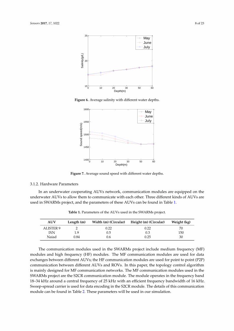
Considering the fact that different hydrological parameters have different effects on thecommunication performance of an underwater cooperating AUVs network, we present thehydrological parameters of the test location in this section. These hydrological parameters, includingthe water temperature, water salinity, and sound speed, are the average values of the test location inpast decades.
Figures 3 and 4 are the yearly average temperature and salinity, respectively, when the waterdepth is 10 m. Figures 5 and 6 are the average temperature and salinity for different water depths andmonths. Figure 7 illustrates the average sound speed in different months with different water depths.

Sensors 2017, 17, 1022 7 of 23Sensors 2017, 17, 1022 7 of 23
Jan Feb Mar Apr May Jun Jul Aug Sep Oct Nov Dec0
5
10
15
20
25
30
Month
Tm
ep
era
ture
de
gre
e
Figure 3. Average temperature in a year.
Jan Feb Mar Apr May Jun Jul Aug Sep Oct Nov Dec0
5
10
15
20
25
30
Month
Sa
linity(g
/L)
Figure 4. Average salinity in a year.
0 10 20 30 50 600
5
10
15
20
25
30
Depth(m)
Te
mp
era
ture
May
June
July
Figure 5. Average temperature with different water depths.
Figure 3. Average temperature in a year.
Sensors 2017, 17, 1022 7 of 23
Jan Feb Mar Apr May Jun Jul Aug Sep Oct Nov Dec0
5
10
15
20
25
30
Month
Tm
ep
era
ture
de
gre
e
Figure 3. Average temperature in a year.
Jan Feb Mar Apr May Jun Jul Aug Sep Oct Nov Dec0
5
10
15
20
25
30
Month
Sa
linity(g
/L)
Figure 4. Average salinity in a year.
0 10 20 30 50 600
5
10
15
20
25
30
Depth(m)
Te
mp
era
ture
May
June
July
Figure 5. Average temperature with different water depths.
Figure 4. Average salinity in a year.
Sensors 2017, 17, 1022 7 of 23
Jan Feb Mar Apr May Jun Jul Aug Sep Oct Nov Dec0
5
10
15
20
25
30
Month
Tm
ep
era
ture
de
gre
e
Figure 3. Average temperature in a year.
Jan Feb Mar Apr May Jun Jul Aug Sep Oct Nov Dec0
5
10
15
20
25
30
Month
Sa
linity(g
/L)
Figure 4. Average salinity in a year.
0 10 20 30 50 600
5
10
15
20
25
30
Depth(m)
Te
mp
era
ture
May
June
July
Figure 5. Average temperature with different water depths. Figure 5. Average temperature with different water depths.
Sensors 2017, 17, 1022 8 of 23Sensors 2017, 17, 1022 8 of 23
0 10 20 30 50 6015
20
25
Depth(m)
Sa
linity(g
/L)
May
June
July
Figure 6. Average salinity with different water depths.
0 10 20 30 50 601400
1450
1500
1550
1600
Depth(m)
So
un
d s
pe
ed
(m/s
)
May
June
July
Figure 7. Average sound speed with different water depths.
3.1.2. Hardware Parameters
In an underwater cooperating AUVs network, communication modules are equipped on the
underwater AUVs to allow them to communicate with each other. Three different kinds of AUVs are
used in SWARMs project, and the parameters of these AUVs can be found in Table 1.
Table 1. Parameters of the AUVs used in the SWARMs project.
AUV Length (m) Width (m) (Circular) Height (m) (Circular) Weight (kg)
ALISTER 9 2 0.22 0.22 70
IXN 1.9 0.5 0.3 150
Naiad 0.84 0.6 0.25 30
The communication modules used in the SWARMs project include medium frequency (MF)
modules and high frequency (HF) modules. The MF communication modules are used for data
exchanges between different AUVs; the HF communication modules are used for point to point
(P2P) communication between different AUVs and ROVs. In this paper, the topology control
algorithm is mainly designed for MF communication networks. The MF communication modules
used in the SWARMs project are the S2CR communication module. The module operates in the
frequency band 18–34 kHz around a central frequency of 25 kHz with an efficient frequency
bandwidth of 16 kHz. Sweep-spread carrier is used for data encoding in the S2CR module. The
details of this communication module can be found in Table 2. These parameters will be used in our
simulation.
Figure 6. Average salinity with different water depths.
Sensors 2017, 17, 1022 8 of 23
0 10 20 30 50 6015
20
25
Depth(m)
Sa
linity(g
/L)
May
June
July
Figure 6. Average salinity with different water depths.
0 10 20 30 50 601400
1450
1500
1550
1600
Depth(m)
So
un
d s
pe
ed
(m/s
)
May
June
July
Figure 7. Average sound speed with different water depths.
3.1.2. Hardware Parameters
In an underwater cooperating AUVs network, communication modules are equipped on the
underwater AUVs to allow them to communicate with each other. Three different kinds of AUVs are
used in SWARMs project, and the parameters of these AUVs can be found in Table 1.
Table 1. Parameters of the AUVs used in the SWARMs project.
AUV Length (m) Width (m) (Circular) Height (m) (Circular) Weight (kg)
ALISTER 9 2 0.22 0.22 70
IXN 1.9 0.5 0.3 150
Naiad 0.84 0.6 0.25 30
The communication modules used in the SWARMs project include medium frequency (MF)
modules and high frequency (HF) modules. The MF communication modules are used for data
exchanges between different AUVs; the HF communication modules are used for point to point
(P2P) communication between different AUVs and ROVs. In this paper, the topology control
algorithm is mainly designed for MF communication networks. The MF communication modules
used in the SWARMs project are the S2CR communication module. The module operates in the
frequency band 18–34 kHz around a central frequency of 25 kHz with an efficient frequency
bandwidth of 16 kHz. Sweep-spread carrier is used for data encoding in the S2CR module. The
details of this communication module can be found in Table 2. These parameters will be used in our
simulation.
Figure 7. Average sound speed with different water depths.
3.1.2. Hardware Parameters
In an underwater cooperating AUVs network, communication modules are equipped on theunderwater AUVs to allow them to communicate with each other. Three different kinds of AUVs areused in SWARMs project, and the parameters of these AUVs can be found in Table 1.
Table 1. Parameters of the AUVs used in the SWARMs project.
AUV Length (m) Width (m) (Circular) Height (m) (Circular) Weight (kg)
ALISTER 9 2 0.22 0.22 70IXN 1.9 0.5 0.3 150
Naiad 0.84 0.6 0.25 30
The communication modules used in the SWARMs project include medium frequency (MF)modules and high frequency (HF) modules. The MF communication modules are used for dataexchanges between different AUVs; the HF communication modules are used for point to point (P2P)communication between different AUVs and ROVs. In this paper, the topology control algorithmis mainly designed for MF communication networks. The MF communication modules used in theSWARMs project are the S2CR communication module. The module operates in the frequency band18–34 kHz around a central frequency of 25 kHz with an efficient frequency bandwidth of 16 kHz.Sweep-spread carrier is used for data encoding in the S2CR module. The details of this communicationmodule can be found in Table 2. These parameters will be used in our simulation.

Sensors 2017, 17, 1022 9 of 23
Table 2. Parameters of the S2CR communication module.
Items Parameters
Operating depth 200 m to 2000 m depending on the housing material; 6000 m for Ti
Operating range 3500 m
Frequency band 18–34 kHz
Transducer beam pattern Horizontally omnidirectional
Acoustic connection (1) Burst data mode: up to 13.9 kbit/s in good channel conditions; 2.2–3.2 kbit/s incomplex channel condition shallow water; (2) instant message mode: 1 kbit/s
Bit error rate Less than 10−10
Power Stand-by mode: 2.5 mW; listen mode: 5–285 mW; receive mode: ≤1.3 W; transmissionmode: 2.8 W (1000 m), 8 W (2000 m), 35 W (3500 m), 80 W (max available)
Power supply External 24 VDC; internal rechargeable battery
Dimensions diameter 110 mm; total length 265 mm
3.1.3. The Sweep-Spread Carrier Model
The S2CR module shown in Table 2 is built upon the sweep-spread carrier (S2C) technology [31].In the following, we will introduce this technology under multipath environment and Dopplerspreading environment briefly.
Digital Signal with Sweep Spread Carrier
Assuming that the sweep spread carrier (S2-carrier) consists of a succession of sweeps withfrequency variation from ωL to ωH within a time interval Tsw, and all the sweeps will be uniformlyproduced in a linear manner with rapid frequency variation following each other successively withoutany gap between them. Then the S2-carrier can be expressed as:
c(t) = Acej(ωL(t−b tTsw cTsw)+m(t−b t
Tsw cTsw)2), (1)
where Ac is the amplitude; m = (ωH−ωL)2Tsw
is a coefficient denoting the frequency variation rate; ωL andωH denote the lowest and highest angular frequencies, respectively; Tsw is the sweep duration; the term⌊
tTsw
⌋denotes the operand for truncating the value to the nearest least integer, which is defined as:
(t−⌊
tTsw
⌋Tsw
)=
{t
Tsw
}Tsw, (2)
Equation (2) can be interpreted in Equation (1) as an actual cycle time with the cycle duration Tsw.
Signal with Sweep Spread Carrier under Multipath Channel
Based on the conclusions in Equations (1) and (2), the signal with S2C in a multipath channel canbe calculated. Let the symbol s(t) be phase encoded data. The symbols are modulated onto the S2C,which is x(t) = s(t) · c(t). The signal is transmitted over a dispersive underwater channel. The part ofthe model which represents the water medium consists of a number of delay elements τi which denotethe time intervals between two successive multipath arrivals, and a number of multiplication elementsVi which takes possible attenuations on interfering multipath arrivals into account.
If both c(t) and s(t) have unit amplitudes, and every coefficient Vi and delay element τiremain constant during the entire transmission time, then after propagation along different paths inan underwater medium, the signals received by a receiver can be calculated as:
y(t) = V0x(t) + ∑i
Vix(t− τi) + n(t), (3)

Sensors 2017, 17, 1022 10 of 23
where x(t) is defined as above, and x(t− τi) can be expressed as:
x(t− τi) = s(t− τi) · ej(ωL{t−τiTsw }Tsw+m({ t−τi
Tsw }Tsw)2), (4)
where n(t) is the white noise. It is evident that:{t− τiTsw
}Tsw =
{tc − τci, tc ≥ τciTsw + tc − τci, tc < τci
, (5)
where tc ={
tTsw
}Tsw is the cycle time defined in Equation (2), and τci =
{τi
Tsw
}Tsw is a fractional part
of time delay related to sweep duration Tsw. Thus, every delayed arrival represented in the secondmember of Equation (3) can be rewritten as:
x(t− τi) =
{s(t− τi) · ej(ωL(tc−τci)+m(tc−τci)
2), tc ≥ τci
s(t− τi) · ej(ωL(Tsw+tc−τci)+m(Tsw+tc−τci)2), tc < τci
, (6)
After transformation of Equation (6), each delayed arrival can be written as:
x(t− τi) = s(t− τi) · ej(ωLtc+mt2c ) · ej(−∆ωitc+φi), (7)
where ∆ωi =
{2mτci, tc ≥ τci−2m(Tsw − τci), tc < τci
is the frequency deviation of the i-th multipath arrival
caused by delay τi, and φi =
{(mτci −ωL)τci, tc ≥ τci
(ωL + ωL − 2mτci)Tsw−τci
2 , tc < τciis the phase of the i-th
multipath arrival.The term with i = 0 in Equation (3) represents an attenuated version of the original signal, and the
other term is the multipath diversity of its delayed, attenuated and frequency shifted reproductions.The most important feature of Equation (7) is that at any instant all the interfering multipath arrivalshave different frequencies spaced by ∆ωi from each other.
Signal with Sweep Spread Carrier under Doppler Spreading
The same can be shown for time-varying channels. The sweep spread carrier under Dopplerspreading can be expressed as [31]:
x(t− τi) = s(t− τi) · ej(ωL{t−τiTsw }Tsw+m({ t−τi
Tsw }Tsw)2) · ejωi
d(t−τi), (8)
where ωid is the Doppler frequency encountered in i-th propagation path, which reflects the influence
of Doppler effection on the received signal. The last exponent in Equation (8) can reflect time-varyingphase/frequency. In this case, the ωi
d is characterized with a time dependent function specific for i-thpath induced. Equation (8) demonstrates that Doppler shifts belonging to different paths will not becoupled while the ωi
d stays within certain borders; so a maximum value ωidmax of the time-varying
bandwidth enlargement ωid does not extend a half of frequency separation space between respective
multipath arrivals (e.g., ωidmax <
ωid
2 ). In this case, every arrival stays within a definite frequency rangeand does not influence another frequency bands; no inter-modulation between differently varyingDoppler terms belonging to different propagation paths takes place.

Sensors 2017, 17, 1022 11 of 23
3.1.4. Propagation Model
According to the conclusion in [32], the path loss model of underwater acoustic channel over adistance l with signal frequency f is given as:
A(l, f ) = lka( f )l , (9)
where k is the spreading factor, a( f ) is the absorption coefficient. The pass loss model shown inEquation (9) can be expressed in dB, which is given by:
10 log A(l, f ) = k · 10 log l + l · 10 log a( f ), (10)
where k · 10 log l is the spreading loss; l · 10 log a( f ) means the absorption loss. The k is the spreadingfactor which describes the geometry of propagation and the values are: (1) k = 2 for sphericalspreading; (2) k = 1 for cylindrical spreading; (3) k = 1.5 for practical spreading.
The absorption coefficient a( f ) can be expressed by using Thorp’s formula, which is an empiricalformula; the a( f ) can be expressed as:
10 log a( f ) = 0.11× f 2
1 + f 2 + 44× f 2
4100 + f 2 + 2.75× 10⁻⁴ f 2 + 0.003, (11)
Equation (11) is used for frequencies above a few hundred Hz. If the frequencies are low,then Equation (11) can be rewritten as:
10 log a( f ) = 0.11× f 2
1 + f 2 + 0.011 f 2 + 0.002, (12)
Therefore, when the transmission power is P, the received signal power will be:
Pr =P
A(l, f )=
P
lka( f )l , (13)
According to Equation (13), when the received signal power is equal to the receive threshold Prth,the transmission range r of this AUV can be calculated based on Equation (13).
3.1.5. Network Model
In the use case of detection, inspection and traction of plumes, the underwater AUVs are deployedapproximately in a 2-dimensional plane. An AUV can move based on a predefined path, as shownin Figure 2. Each AUV in the network can communicate with other AUVs whose distances to thisAUV are smaller than its transmission range. For instance, as shown in Figure 8, AUV s and AUVd can communicate with each other when ‖sd‖ ≤ rs, where ‖sd‖ is the Euclidean distance betweenAUV s and AUV d, and rs is the transmission range of AUV s. The AUVs in network can adjust theirtransmission power from 0 to Pmax, which can be found in Table 2. The coverage area of AVU s isa circle where the centre is AUV s and the radius is rs, denoted as C(s, rs). This is shown in Figure 8.The number of one-hop neighbor AUVs in the coverage area of AUV s is defined as the degree of AUVs. For instance, in Figure 8, the degree of AUV s is 7.

Sensors 2017, 17, 1022 12 of 23Sensors 2017, 17, 1022 12 of 23
s
d
sr
Figure 8. The network model of PTC algorithm.
3.2. Parameter Deviation Calculation
In an underwater cooperating AUVs network, the underwater AUVs are always powered by
batteries. Moreover, once the energy is exhausted, the AUVs become non-functional, which has a
great effect on network performance. Similarly to the energy, the buffer space of the underwater
AUVs is limited, too. Thus, in case the memory space is occupied completely, the nodes cannot
handle the incoming data packets, which makes the packet loss ratio increase. The occupation of the
buffer space can be evaluated by queue length (in this paper, the queue length is defined as the
number of data packets to be transmitted in AUV’s buffer space). Therefore, in this paper, the
residual energy, the queue length, the transmission power, and the AUV’s degree will be taken into
account to determine the transmission power adjustment probability for each AUV.
Based on the analysis in Section 1, we define the parameter deviation in Definition 1. The
deviation of a parameter relates to the optimal solution or the constraint of this parameter.
Definition 1. The deviation of parameter x which relates to its optimal solution or constraint *x is defined as
the ratio of the difference between these two values to the value of the optimal solution or the constraint, which
can be expressed as:
*
*
x xD
x
, (14)
According to Definition 1, to transmission power, when the optimal transmission power of
AUV s is *
sP which is calculated by the optimization algorithm, the deviation of transmission
power can be calculated as:
*
*s
s s
P
s
P PD
P
, (15)
Similarly to the transmission power, for the queue length (in this paper, the queue length is
defined as the number of data packets to be transmitted in AUV’s buffer space), assuming that the
maximum queue length allowed in AUV is *
sQ , and the current queue length of AUV s is sQ , then
according to Equation (14), the deviation of queue length is expressed as:
*
*s
s s
Q
s
Q QD
Q
, (16)
The total energy of AUV is *
sE and the residual energy of AUV s is sE , then the deviation of
residual energy is:
Figure 8. The network model of PTC algorithm.
3.2. Parameter Deviation Calculation
In an underwater cooperating AUVs network, the underwater AUVs are always powered bybatteries. Moreover, once the energy is exhausted, the AUVs become non-functional, which hasa great effect on network performance. Similarly to the energy, the buffer space of the underwaterAUVs is limited, too. Thus, in case the memory space is occupied completely, the nodes cannothandle the incoming data packets, which makes the packet loss ratio increase. The occupation ofthe buffer space can be evaluated by queue length (in this paper, the queue length is defined as thenumber of data packets to be transmitted in AUV’s buffer space). Therefore, in this paper, the residualenergy, the queue length, the transmission power, and the AUV’s degree will be taken into account todetermine the transmission power adjustment probability for each AUV.
Based on the analysis in Section 1, we define the parameter deviation in Definition 1. The deviationof a parameter relates to the optimal solution or the constraint of this parameter.
Definition 1. The deviation of parameter x which relates to its optimal solution or constraint x∗ is defined as theratio of the difference between these two values to the value of the optimal solution or the constraint, which canbe expressed as:
D =|x− x∗|
x∗, (14)
According to Definition 1, to transmission power, when the optimal transmission power of AUV sis P∗s which is calculated by the optimization algorithm, the deviation of transmission power can becalculated as:
DPs =|Ps − P∗s |
P∗s, (15)
Similarly to the transmission power, for the queue length (in this paper, the queue length is definedas the number of data packets to be transmitted in AUV’s buffer space), assuming that the maximumqueue length allowed in AUV is Q∗s , and the current queue length of AUV s is Qs, then according toEquation (14), the deviation of queue length is expressed as:
DQs =|Qs −Q∗s |
Q∗s, (16)
The total energy of AUV is E∗s and the residual energy of AUV s is Es, then the deviation ofresidual energy is:
DEs =|Es − E∗s |
E∗s, (17)

Sensors 2017, 17, 1022 13 of 23
Assuming that the needed degree of AUV for guaranteeing network connection is n∗s and thecurrent degree of AUV is ns, then the deviation of AUV’s degree can be calculated as:
DEs =|ns − n∗s |
n∗s, (18)
Note that in Equation (18), the AUV degree needed for guaranteeing network connections can becalculated based on the conclusion in [33]. In [33], the authors have proved that for a wireless network,if the number of neighbors of a node is larger than 5.1774 log n, then the network will be connectedwith probability 1; where n is the total number of nodes in network, so in this paper, considering theenergy consumption, we choose n∗s = 5.1774 log n as the needed AUV degree.
3.3. Transmission Power Adjustment Probability Calculation
When the parameter deviations have been determined, the transmission range adjustmentprobability can be calculated based on these deviations. The transmission range adjustment probabilityis defined in Definition 2.
Definition 2. In an underwater cooperating AUVs network, considering the tradeoff between improvingthe network performance as one aspect and keeping the function of AUVs, the AUVs, in which the currenttransmission power does not equal the optimal transmission power that is calculated based on optimal algorithms,do not need to adjust their transmission power; rather the AUVs change their transmission power probability.This probability is called the transmission power adjustment probability.
The calculation of the transmission power adjustment probability is based on the value of theparameter deviations. The larger the deviation, the larger the probability is. Since the mathematicalrelationship between the transmission power adjustment probability and the parameter deviationcannot be defined clearly, in this paper, we use the fuzzy logic algorithm to calculate the transmissionpower adjustment probability. The input of the fuzzy logic system is the value of parameter deviation,and output is the transmission power adjustment probability of each parameters.
As introduced in [34], the core part of fuzzy logic system is the fuzzy rules design, which decidesthe accuracy of the output. The more fuzzy rules are applied, the more accurate outputs are. Therefore,similarly to [34], the number of fuzzy rules used in this paper is set to 7, which are shown in Table 3.
Table 3. The Fuzzy rules.
INPUT (If): Parameter Deviation OUTPUT (Then): Adjustment Probability
Very small Very smallMedium small Medium small
Small SmallMedium Medium
Large LargeMedium large Medium large
Very large Very large
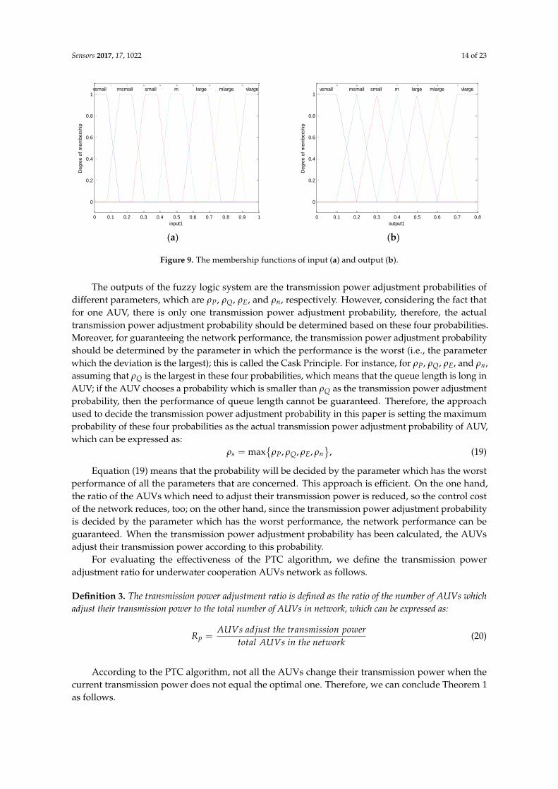
The membership functions of inputs and outputs are shown in Figure 9.
Sensors 2017, 17, 1022 14 of 23Sensors 2017, 17, 1022 14 of 23
0 0.1 0.2 0.3 0.4 0.5 0.6 0.7 0.8 0.9 1
0
0.2
0.4
0.6
0.8
1
input1
Degre
e o
f m
em
bers
hip
vsmall msmall small m large mlarge vlarge
(a)
0 0.1 0.2 0.3 0.4 0.5 0.6 0.7 0.8
0
0.2
0.4
0.6
0.8
1
output1
Degre
e o
f m
em
bers
hip
vsmall msmall small m large mlarge vlarge
(b)
Figure 9. The membership functions of input (a) and output (b).
The outputs of the fuzzy logic system are the transmission power adjustment probabilities of
different parameters, which are P , Q , E , and n , respectively. However, considering the fact
that for one AUV, there is only one transmission power adjustment probability, therefore, the actual
transmission power adjustment probability should be determined based on these four probabilities.
Moreover, for guaranteeing the network performance, the transmission power adjustment
probability should be determined by the parameter in which the performance is the worst (i.e., the
parameter which the deviation is the largest); this is called the Cask Principle. For instance, for P ,
Q , E , and
n , assuming that Q is the largest in these four probabilities, which means that the
queue length is long in AUV; if the AUV chooses a probability which is smaller than Q as the
transmission power adjustment probability, then the performance of queue length cannot be
guaranteed. Therefore, the approach used to decide the transmission power adjustment probability
in this paper is setting the maximum probability of these four probabilities as the actual
transmission power adjustment probability of AUV, which can be expressed as:
max , , ,s P Q E n , (19)
Equation (19) means that the probability will be decided by the parameter which has the worst
performance of all the parameters that are concerned. This approach is efficient. On the one hand,
the ratio of the AUVs which need to adjust their transmission power is reduced, so the control cost of
the network reduces, too; on the other hand, since the transmission power adjustment probability is
decided by the parameter which has the worst performance, the network performance can be
guaranteed. When the transmission power adjustment probability has been calculated, the AUVs
adjust their transmission power according to this probability.
For evaluating the effectiveness of the PTC algorithm, we define the transmission power
adjustment ratio for underwater cooperation AUVs network as follows.
Definition 3. The transmission power adjustment ratio is defined as the ratio of the number of AUVs which
adjust their transmission power to the total number of AUVs in network, which can be expressed as:
p
AUVs adjust the transmission powerR
total AUVs in the network (20)
According to the PTC algorithm, not all the AUVs change their transmission power when the
current transmission power does not equal the optimal one. Therefore, we can conclude Theorem 1
as follows.
Theorem 1. The PTC algorithm can reduce the transmission power adjustment ratio greatly.
Figure 9. The membership functions of input (a) and output (b).
The outputs of the fuzzy logic system are the transmission power adjustment probabilities ofdifferent parameters, which are ρP, ρQ, ρE, and ρn, respectively. However, considering the fact thatfor one AUV, there is only one transmission power adjustment probability, therefore, the actualtransmission power adjustment probability should be determined based on these four probabilities.Moreover, for guaranteeing the network performance, the transmission power adjustment probabilityshould be determined by the parameter in which the performance is the worst (i.e., the parameterwhich the deviation is the largest); this is called the Cask Principle. For instance, for ρP, ρQ, ρE, and ρn,assuming that ρQ is the largest in these four probabilities, which means that the queue length is long inAUV; if the AUV chooses a probability which is smaller than ρQ as the transmission power adjustmentprobability, then the performance of queue length cannot be guaranteed. Therefore, the approachused to decide the transmission power adjustment probability in this paper is setting the maximumprobability of these four probabilities as the actual transmission power adjustment probability of AUV,which can be expressed as:
ρs = max{
ρP, ρQ, ρE, ρn}
, (19)
Equation (19) means that the probability will be decided by the parameter which has the worstperformance of all the parameters that are concerned. This approach is efficient. On the one hand,the ratio of the AUVs which need to adjust their transmission power is reduced, so the control costof the network reduces, too; on the other hand, since the transmission power adjustment probabilityis decided by the parameter which has the worst performance, the network performance can beguaranteed. When the transmission power adjustment probability has been calculated, the AUVsadjust their transmission power according to this probability.
For evaluating the effectiveness of the PTC algorithm, we define the transmission poweradjustment ratio for underwater cooperation AUVs network as follows.
Definition 3. The transmission power adjustment ratio is defined as the ratio of the number of AUVs whichadjust their transmission power to the total number of AUVs in network, which can be expressed as:
Rp =AUVs adjust the transmission power
total AUVs in the network(20)
According to the PTC algorithm, not all the AUVs change their transmission power when thecurrent transmission power does not equal the optimal one. Therefore, we can conclude Theorem 1as follows.

Sensors 2017, 17, 1022 15 of 23
Theorem 1. The PTC algorithm can reduce the transmission power adjustment ratio greatly.
Proof. According to Equation (19), in PTC algorithm, the transmission power adjustment probabilityof AUV s is ρs. Assuming that there are n AUVs in network and the number of AUVs which thetransmission power does not equal to the optimal one is ns; therefore, the average number of AUVswhich adjust their transmission power can be calculated as:
E(ns) =ns
∑i=1
ρi, (21)
Then according to Definition 2, the transmission power adjustment ratio of the PTC algorithmcan be calculated as:
Rp =E(ns)
n=
ns∑
i=1ρi
n, (22)
However, in traditional topology control algorithms, once the transmission power does notequal to the optimal one, the AUVs need to adjust their transmission power. Since the number ofAUVs which the transmission power does not equal to the optimal one is ns, the transmission poweradjustment ratio of the traditional topology control algorithm can be calculated as:
Rp =ns
n, (23)
Since ρi < 1, so the Rp in Equation (23) is larger than that in Equation (22); moreover, the smallerρs, the smaller Rp is. Therefore, the transmission power adjustment ratio in PTC algorithm is smallerthan that in traditional topology control algorithm.
3.4. PTC-Based FTC Algorithm
Based on Sections 3.2 and 3.3, the transmission power adjustment probability of AUV can becalculated. After that, the AUVs will adjust their transmission power according to this probability.
Since many transmission power allocation algorithms have been proposed in the past decades,the transmission power allocation algorithm will be not the main research topic of this paper. In thispaper, the calculation of the optimal transmission power is based on the FTC algorithm which isproposed by [6]. The FTC algorithm is the learning-based fuzzy logic control algorithm for topologycontrol. In the following, we will introduce this algorithm briefly.
Figure 10 shows the system structure of FTC. Adjusting the communication power is a verycommon capability of many AUVs. The output of FTC is the transmission power (TP). The target ofFTC is to reach a specific degree of AUVs. Therefore, the input is the desired AUV’s degree, denoted byNDre f . On the other hand, according to the conclusion in [35], the probability that AUV’s degree is n isshown in Equation (24), so the probability that an AUV has n neighbors is another fuzzy logic controllerinput, denoted by Prob. In practice, NDre f is integer and the transmission power has an upper boundPmax, i.e., NDre f > 0 and 0 ≤ P ≤ Pmax:
P(ND ≥ k) = f (k, P) = 1−k−1
∑n=0
(ρπr2)n
n!e−ρπr2
, (24)

Sensors 2017, 17, 1022 16 of 23Sensors 2017, 17, 1022 16 of 23
Fuzzy Logic
Controler
Training data set
AUVs
refND k
NDeK
Prob
0Prob
TP ND
Figure 10. The fuzzy-logic topology control (FTC) scheme.
The training data set is provided by Equation (24); the fuzzy controller can be obtained through
the neuro-adaptive learning algorithm. In Equation (24), the transmission range can be calculated
based on Equation (13). The parameters of the membership function are automatically tuned
through a back propagation algorithm individually or in combination with a least squares method.
The generation of the training data set can be shown as follows. As illustrated in Figure 10 and
Equation (24), the inputs are refND and Prob, and the output is the transmission power. Given ,
1 2, ,..., mND k k k and 1 2, ,..., mTP p p p , ( , )Prob f ND TP can be calculated from Equation (24).
The training data set T is a 3s matrix in the form of [ , , ]ND Prob TP , where s m j . For instance,
one element in the training data set is (3, 0.9, 0.25); this means that the transmission power is set to
0.25 if the probability that 3ND is 0.9, where the transmission power is normalized (i.e., the
maximum transmission power is (1). Since ND is characterized by probability, it is necessary to
adjust the AUV’s degree if an AUV does not reach ND. For instance if TP = 0.25 cannot actually lead
to k = ND, then the next step is to adjust Prob to a higher value according to the AUV’s degree error
NDe . There is an integral controller outside the fuzzy control to adaptively change Prob (Figure 10).
From the control theory point of view, the system properties are controlled by parameter 0Prob and
K. If NDe is less than 0, K is configured to be half of its initial value. Therefore, according to the FTC
algorithm, the process of the PTC based FTC algorithm can be expressed as follows:
Step 1: Getting the optimal transmission power *P based on an optimal transmission power
allocation algorithm, such as the FTC algorithm [6];
Step 2: Calculating the deviations of each parameter, which are PD , QD , ED , and nD ;
Step 3: Calculating the transmission power adjust probabilities based on the parameter deviations
calculated in Step 2 and the fuzzy logic system shown in Section 3.3; the transmission
power adjustment probabilities of parameters are P , Q , E , and n ;
Step 4: Finding the maximum transmission power adjustment probability of , , ,P Q E n and
setting this probability as the transmission power adjustment probability of the AUV;
Step 5: Adjusting the transmission power of the AUV based on the probability calculated in Step 4
and the optimal transmission power *P calculated in Step 1.
The PTC-based FTC algorithm can be found in Algorithm 1.
Algorithm 1. PTC-based FTC algorithm
Inputs:
1. Training data set, ( , , )T k Prob TP ;
2. Maximum transmission power, maxP ;
3. Reference degree of AUV, refND ;
4. Initial probability, 0Prob ;
5. Initial K, K0;
6. The maximum queue length, Q;
7. The maximum residual energy, E:
Figure 10. The fuzzy-logic topology control (FTC) scheme.
The training data set is provided by Equation (24); the fuzzy controller can be obtained through theneuro-adaptive learning algorithm. In Equation (24), the transmission range can be calculated basedon Equation (13). The parameters of the membership function are automatically tuned through a backpropagation algorithm individually or in combination with a least squares method. The generation ofthe training data set can be shown as follows. As illustrated in Figure 10 and Equation (24), the inputsare NDre f and Prob, and the output is the transmission power. Given ρ, ND ∈ {k1, k2, . . . , km} andTP ∈ {p1, p2, . . . , pm}, Prob = f (ND, TP) can be calculated from Equation (24). The training data setT is a s× 3 matrix in the form of [ND, Prob, TP], where s = m · j. For instance, one element in thetraining data set is (3, 0.9, 0.25); this means that the transmission power is set to 0.25 if the probabilitythat ND ≥ 3 is 0.9, where the transmission power is normalized (i.e., the maximum transmissionpower is (1). Since ND is characterized by probability, it is necessary to adjust the AUV’s degree ifan AUV does not reach ND. For instance if TP = 0.25 cannot actually lead to k = ND, then the nextstep is to adjust Prob to a higher value according to the AUV’s degree error eND. There is an integralcontroller outside the fuzzy control to adaptively change Prob (Figure 10). From the control theorypoint of view, the system properties are controlled by parameter Prob0 and K. If eND is less than 0, K isconfigured to be half of its initial value. Therefore, according to the FTC algorithm, the process of thePTC based FTC algorithm can be expressed as follows:
Step 1: Getting the optimal transmission power P∗ based on an optimal transmission power allocationalgorithm, such as the FTC algorithm [6];
Step 2: Calculating the deviations of each parameter, which are DP, DQ, DE, and Dn;Step 3: Calculating the transmission power adjust probabilities based on the parameter deviations
calculated in Step 2 and the fuzzy logic system shown in Section 3.3; the transmission poweradjustment probabilities of parameters are ρP, ρQ, ρE, and ρn;
Step 4: Finding the maximum transmission power adjustment probability of{
ρP, ρQ, ρE, ρn}
andsetting this probability as the transmission power adjustment probability of the AUV;
Step 5: Adjusting the transmission power of the AUV based on the probability calculated in Step 4 andthe optimal transmission power P∗ calculated in Step 1.
The PTC-based FTC algorithm can be found in Algorithm 1.

Sensors 2017, 17, 1022 17 of 23
Algorithm 1. PTC-based FTC algorithm
Inputs:
1. Training data set, T = (k, Prob, TP);2. Maximum transmission power, Pmax;3. Reference degree of AUV, NDre f ;
4. Initial probability, Prob0;5. Initial K, K0;6. The maximum queue length, Q;7. The maximum residual energy, E:8. TPi ⇐ Pmax ;9. Prob⇐ Prob0 ;10. Broadcast HELLO message with current TPi;11. For messages received from other AUVs, store the ID of its neighbor AUVs;12. Calculate the number of neighbors ND in the neighbor list;13. Calculate eND = ND− NDre f ;
14. if eND < 0 then15. K = K0;16. else
17. K = K02 ;
18. end if19. Prob⇐ Prob− K · eND ;20. TPi ⇐ FTC(NDre f , Prob) ;
21. Calculate the deviations DPs , DQs , DEs , Dns ;22. Input the deviations into the fuzzy logic system to calculate the transmission power adjustment
probability ρP, ρQ, ρE, and ρn;23. ρs ⇐ max
{ρP, ρQ, ρE, ρn
};
24. Adjust the transmission power according to ρs (random decision based on the probability value).
Note that in this paper, the PTC algorithm is combined with the FTC algorithm; however,in practice, the PTC algorithm can be combined with other different topology control algorithmsto improve the performance and reduce the transmission power adjustment ratio.
4. Simulation and Discussion
In this section, we will evaluate the performance of PTC algorithm by simulation. To highlight theoutstanding qualities of the PTC algorithm, we combine the PTC with the FTC algorithm and comparethe performance of FTC algorithm with the PTC-FTC algorithm. The simulation results shown in [6]have demonstrated that the FTC algorithm is highly efficient in controlling the network topology.
4.1. Simulation Configuration
Based on the communication architecture of SWARMs project shown in Section 3.1, the simulationconfiguration parameters of the underwater cooperating AUVs network is shown in Table 4.

Sensors 2017, 17, 1022 18 of 23
Table 4. Simulation configuration.
Parameters Value
Simulation tool DESERT 1
Simulation area 3000 m × 3000 mNumber of AUVs 3, 5, 7, 9, 11, 13
Depth 20 mWater temperature (July) 12 ◦C
Water salinity (July) 18 g/LSound speed (July) 1475 m/s
Initial transmission range 1000 mTransducer beam pattern Horizontally Omni-directional
Data rate 3 kbit/sBit error ratio 10−10
Receive power 1.3 WTransmission power 2.8 W
Channel model Multi-path + Doppler spreadingCarrier Sweep spread carrier (S2C)
1 DESERT: http://nautilus.dei.unipd.it/desert-underwater.
4.2. Simulation Results
The simulation results can be found from Figures 11–15. The simulation tool is DESER, which isan extension toolbox based on the NS-2 simulator. The simulation parameters can be found inSections 3.1 and 4.1.
In Figure 11, the average transmission power adjustment probability of the AUV is shown.From this figure we can find that this probability varies between 0.4 and 0.5. When the number ofAUVs increases, there is no evidence showing that the transmission power adjustment probabilityincreases too. This is because the probability is determined by the residual energy, the transmissionpower, the node degree, and the queue length jointly, so an increasing of the number of AUVs in thenetwork cannot affect the probability greatly.
Sensors 2017, 17, 1022 18 of 23
Receive power 1.3 W
Transmission power 2.8 W
Channel model Multi-path + Doppler spreading
Carrier Sweep spread carrier (S2C)
1 DESERT: http://nautilus.dei.unipd.it/desert-underwater.
4.2. Simulation Results
The simulation results can be found from Figures 11–15. The simulation tool is DESER, which is
an extension toolbox based on the NS-2 simulator. The simulation parameters can be found in
Sections 3.1 and 4.1.
In Figure 11, the average transmission power adjustment probability of the AUV is shown.
From this figure we can find that this probability varies between 0.4 and 0.5. When the number of
AUVs increases, there is no evidence showing that the transmission power adjustment probability
increases too. This is because the probability is determined by the residual energy, the transmission
power, the node degree, and the queue length jointly, so an increasing of the number of AUVs in the
network cannot affect the probability greatly.
3 5 7 9 11 130
0.1
0.2
0.3
0.4
0.5
0.6
0.7
0.8
Number of AUVs
Tra
nsm
issio
n p
ow
er
ad
justm
en
t p
rob
ab
ility
Figure 11. The average transmission power adjustment probability of PTC-FTC.
3 5 7 9 11 130.4
0.6
0.8
1
1.2
Number of AUVs
Tra
nsm
ssio
n P
ow
er
ad
justm
en
t ra
tio
PTC-FTC
FTC
Figure 12. The average transmission power adjustment ratio of PTC-FTC and FTC.
Figure 11. The average transmission power adjustment probability of PTC-FTC.

Sensors 2017, 17, 1022 19 of 23
Sensors 2017, 17, 1022 18 of 23
Receive power 1.3 W
Transmission power 2.8 W
Channel model Multi-path + Doppler spreading
Carrier Sweep spread carrier (S2C)
1 DESERT: http://nautilus.dei.unipd.it/desert-underwater.
4.2. Simulation Results
The simulation results can be found from Figures 11–15. The simulation tool is DESER, which is
an extension toolbox based on the NS-2 simulator. The simulation parameters can be found in
Sections 3.1 and 4.1.
In Figure 11, the average transmission power adjustment probability of the AUV is shown.
From this figure we can find that this probability varies between 0.4 and 0.5. When the number of
AUVs increases, there is no evidence showing that the transmission power adjustment probability
increases too. This is because the probability is determined by the residual energy, the transmission
power, the node degree, and the queue length jointly, so an increasing of the number of AUVs in the
network cannot affect the probability greatly.
3 5 7 9 11 130
0.1
0.2
0.3
0.4
0.5
0.6
0.7
0.8
Number of AUVs
Tra
nsm
issio
n p
ow
er
ad
justm
en
t p
rob
ab
ility
Figure 11. The average transmission power adjustment probability of PTC-FTC.
3 5 7 9 11 130.4
0.6
0.8
1
1.2
Number of AUVs
Tra
nsm
ssio
n P
ow
er
ad
justm
en
t ra
tio
PTC-FTC
FTC
Figure 12. The average transmission power adjustment ratio of PTC-FTC and FTC. Figure 12. The average transmission power adjustment ratio of PTC-FTC and FTC.Sensors 2017, 17, 1022 19 of 23
3 5 7 9 11 130.6
0.7
0.8
0.9
1
Number of AUVs
Ave
rag
e r
esid
ua
l e
ne
rgy
PTC-FTC
FTC
Figure 13. The average residual energy of PTC-FTC and FTC.
3 5 7 9 11 131
2
3
4
5
6
Number of AUVs
Ave
rag
e d
eg
ree
of A
UV
PTC-FTC
FTC
Figure 14. The average node degree of PTC-FTC and FTC.
3 5 7 9 11 130
1
2
3
4
5
6
7
8
9
10
Number of AUVs
Ave
rag
e q
ue
ue
le
ng
th
PTC-FTC
FTC
Figure 15. The average queue length of PTC-FTC and FTC.
For instance, when the number of AUVs increases, the transmission power decreases and the
residual energy increases, which can be found in Figure 13; however, due to the increase of the
AUV’s degree, the queue length will increase (shown in Figure 15); therefore, the probability may
not increase. The transmission power adjustment ratio can be found in Figure 12.
We can see in Figure 12 that the transmission power adjustment ratio of the PTC-FTC algorithm
is much smaller than that of the FTC algorithm. The transmission power adjustment ratio in the FTC
algorithm is about twice larger than that in the PTC-FTC algorithm. This demonstrates that the PTC
algorithm is efficient at reducing the transmission power adjustment ratio. Similarly to the
transmission power adjustment probability shown in Figure 11, the transmission power adjustment
ratio does not increase with the increasing number of AUVs in the network. The reason is that when
the number of AUVs in the network increases, the number of AUVs which need to adjust their
transmission power increases too; moreover, according to the dynamics of an underwater
Figure 13. The average residual energy of PTC-FTC and FTC.
Sensors 2017, 17, 1022 19 of 23
3 5 7 9 11 130.6
0.7
0.8
0.9
1
Number of AUVs
Ave
rag
e r
esid
ua
l e
ne
rgy
PTC-FTC
FTC
Figure 13. The average residual energy of PTC-FTC and FTC.
3 5 7 9 11 131
2
3
4
5
6
Number of AUVs
Ave
rag
e d
eg
ree
of A
UV
PTC-FTC
FTC
Figure 14. The average node degree of PTC-FTC and FTC.
3 5 7 9 11 130
1
2
3
4
5
6
7
8
9
10
Number of AUVs
Ave
rag
e q
ue
ue
le
ng
th
PTC-FTC
FTC
Figure 15. The average queue length of PTC-FTC and FTC.
For instance, when the number of AUVs increases, the transmission power decreases and the
residual energy increases, which can be found in Figure 13; however, due to the increase of the
AUV’s degree, the queue length will increase (shown in Figure 15); therefore, the probability may
not increase. The transmission power adjustment ratio can be found in Figure 12.
We can see in Figure 12 that the transmission power adjustment ratio of the PTC-FTC algorithm
is much smaller than that of the FTC algorithm. The transmission power adjustment ratio in the FTC
algorithm is about twice larger than that in the PTC-FTC algorithm. This demonstrates that the PTC
algorithm is efficient at reducing the transmission power adjustment ratio. Similarly to the
transmission power adjustment probability shown in Figure 11, the transmission power adjustment
ratio does not increase with the increasing number of AUVs in the network. The reason is that when
the number of AUVs in the network increases, the number of AUVs which need to adjust their
transmission power increases too; moreover, according to the dynamics of an underwater
Figure 14. The average node degree of PTC-FTC and FTC.
Sensors 2017, 17, 1022 20 of 23
Sensors 2017, 17, 1022 19 of 23
3 5 7 9 11 130.6
0.7
0.8
0.9
1
Number of AUVs
Ave
rag
e r
esid
ua
l e
ne
rgy
PTC-FTC
FTC
Figure 13. The average residual energy of PTC-FTC and FTC.
3 5 7 9 11 131
2
3
4
5
6
Number of AUVs
Ave
rag
e d
eg
ree
of A
UV
PTC-FTC
FTC
Figure 14. The average node degree of PTC-FTC and FTC.
3 5 7 9 11 130
1
2
3
4
5
6
7
8
9
10
Number of AUVs
Ave
rag
e q
ue
ue
le
ng
th
PTC-FTC
FTC
Figure 15. The average queue length of PTC-FTC and FTC.
For instance, when the number of AUVs increases, the transmission power decreases and the
residual energy increases, which can be found in Figure 13; however, due to the increase of the
AUV’s degree, the queue length will increase (shown in Figure 15); therefore, the probability may
not increase. The transmission power adjustment ratio can be found in Figure 12.
We can see in Figure 12 that the transmission power adjustment ratio of the PTC-FTC algorithm
is much smaller than that of the FTC algorithm. The transmission power adjustment ratio in the FTC
algorithm is about twice larger than that in the PTC-FTC algorithm. This demonstrates that the PTC
algorithm is efficient at reducing the transmission power adjustment ratio. Similarly to the
transmission power adjustment probability shown in Figure 11, the transmission power adjustment
ratio does not increase with the increasing number of AUVs in the network. The reason is that when
the number of AUVs in the network increases, the number of AUVs which need to adjust their
transmission power increases too; moreover, according to the dynamics of an underwater
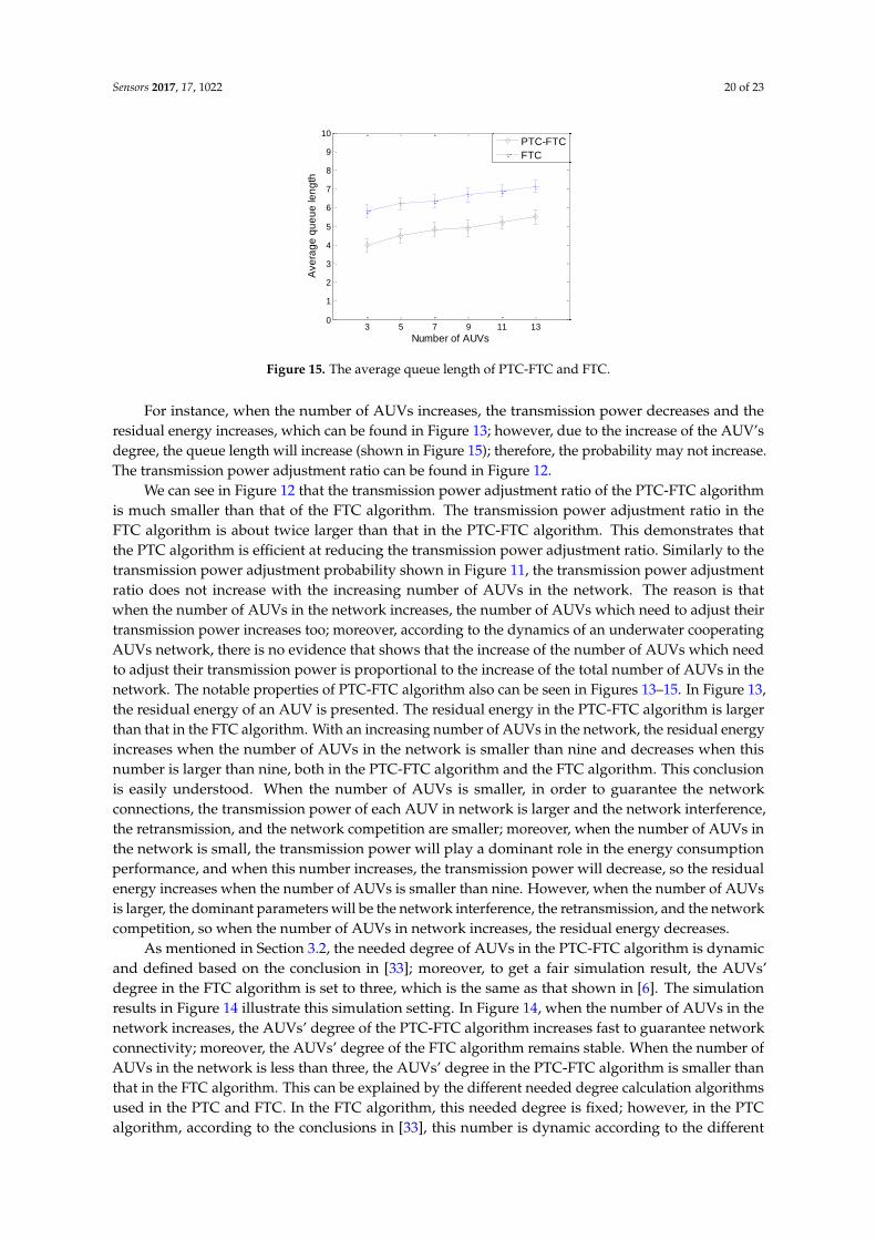
Figure 15. The average queue length of PTC-FTC and FTC.
For instance, when the number of AUVs increases, the transmission power decreases and theresidual energy increases, which can be found in Figure 13; however, due to the increase of the AUV’sdegree, the queue length will increase (shown in Figure 15); therefore, the probability may not increase.The transmission power adjustment ratio can be found in Figure 12.
We can see in Figure 12 that the transmission power adjustment ratio of the PTC-FTC algorithmis much smaller than that of the FTC algorithm. The transmission power adjustment ratio in theFTC algorithm is about twice larger than that in the PTC-FTC algorithm. This demonstrates thatthe PTC algorithm is efficient at reducing the transmission power adjustment ratio. Similarly to thetransmission power adjustment probability shown in Figure 11, the transmission power adjustmentratio does not increase with the increasing number of AUVs in the network. The reason is thatwhen the number of AUVs in the network increases, the number of AUVs which need to adjust theirtransmission power increases too; moreover, according to the dynamics of an underwater cooperatingAUVs network, there is no evidence that shows that the increase of the number of AUVs which needto adjust their transmission power is proportional to the increase of the total number of AUVs in thenetwork. The notable properties of PTC-FTC algorithm also can be seen in Figures 13–15. In Figure 13,the residual energy of an AUV is presented. The residual energy in the PTC-FTC algorithm is largerthan that in the FTC algorithm. With an increasing number of AUVs in the network, the residual energyincreases when the number of AUVs in the network is smaller than nine and decreases when thisnumber is larger than nine, both in the PTC-FTC algorithm and the FTC algorithm. This conclusionis easily understood. When the number of AUVs is smaller, in order to guarantee the networkconnections, the transmission power of each AUV in network is larger and the network interference,the retransmission, and the network competition are smaller; moreover, when the number of AUVs inthe network is small, the transmission power will play a dominant role in the energy consumptionperformance, and when this number increases, the transmission power will decrease, so the residualenergy increases when the number of AUVs is smaller than nine. However, when the number of AUVsis larger, the dominant parameters will be the network interference, the retransmission, and the networkcompetition, so when the number of AUVs in network increases, the residual energy decreases.
As mentioned in Section 3.2, the needed degree of AUVs in the PTC-FTC algorithm is dynamicand defined based on the conclusion in [33]; moreover, to get a fair simulation result, the AUVs’degree in the FTC algorithm is set to three, which is the same as that shown in [6]. The simulationresults in Figure 14 illustrate this simulation setting. In Figure 14, when the number of AUVs in thenetwork increases, the AUVs’ degree of the PTC-FTC algorithm increases fast to guarantee networkconnectivity; moreover, the AUVs’ degree of the FTC algorithm remains stable. When the number ofAUVs in the network is less than three, the AUVs’ degree in the PTC-FTC algorithm is smaller thanthat in the FTC algorithm. This can be explained by the different needed degree calculation algorithmsused in the PTC and FTC. In the FTC algorithm, this needed degree is fixed; however, in the PTCalgorithm, according to the conclusions in [33], this number is dynamic according to the different
Sensors 2017, 17, 1022 21 of 23
network conditions. Interesting conclusions can be found when comparing the simulation results inFigure 13 with those in Figure 14. In Figure 14, the average degree of an AUV in the PTC-FTC algorithmis larger than that in the FTC algorithm; however, the residual energy of the PTC-FTC algorithm islarger than that of the FTC algorithm. This can be explained by the conclusion in Figure 12. Since theprobability adjustment ratio in the PTC-FTC algorithm is smaller than that in the FTC algorithm,the energy consumption for topology control and retransmission caused by network competition issmaller than in the FTC algorithm, so even though the transmission range in the PTC-FTC algorithm islarger than that in the FTC algorithm, the residual energy in the PTC-FTC algorithm is large.
As shown in Figure 15, the queue length of the PTC-FTC algorithm is much smaller than thatof the FTC algorithm, and with an increasing number of AUVs in the network, the queue lengths inboth the PTC-FTC algorithm and FTC algorithm increase. This is because the more AUVs in network,the more data packets need to be transmitted; therefore, the queue length will increase when thenumber of AUVs increases. Additionally, due to the fact the transmission power ratio of the PTC-FTCalgorithm is much smaller than that of the FTC algorithm (which can be seen in Figure 11), the controlmessages in the PTC-FTC algorithm are much smaller than in the FTC algorithm, which means thequeue length in PTC-FTC algorithm is small, too.
The results presented from Figures 11–15 have demonstrated that the PTC-FTC algorithm isefficient on improving network performance while reducing energy consumption for underwatercooperating AUV networks.
5. Conclusions
In this paper, we propose a probabilistic topology control (PTC) algorithm for underwatercooperating AUV networks which are associated with limited communication capability and highmobility. In PTC, to reduce the transmission power adjustment ratio of the topology control algorithm,when the AUVs’ transmission power does not equal the optimal transmission power calculated basedon an optimal algorithm, the AUVs must not adjust their transmission power. The AUV calculates thedeviation of the transmission power, the residual energy, the degree of AUV, and the queue lengthfirstly; then the AUV calculates the transmission power adjustment probabilities of each parameterbased on these deviations. The maximum probability will be chosen as the transmission poweradjustment probability of the AUV. Through this approach, the transmission power adjustment ratioof the topology control algorithm can be reduced greatly (by about 40%). Since the transmission poweradjustment ratio has been reduced, the network performance also improved remarkably.
We note that in this paper, the PTC algorithm is combined with the FTC algorithm; however thePTC algorithm could also be combined with topology control algorithms other than the FTC algorithmto reduce the transmission power adjustment ratio. Additionally, while in this paper, the parameterselection is based on the requirements of the SWARMs project, these parameters are not fixed, and theycan be easily changed based on the requirements of different applications. This flexibility representsone of the main advantages of PTC algorithm.
Acknowledgments: The research leading to the presented results has been undertaken with in the SWARMsEuropean project (Smart and Networking Underwater Robots in Cooperation Meshes), under Grant Agreementn. 662107-SWARMs-ECSEL-2014-1, partially supported by the ECSEL JU and the Spanish Ministry of Economyand Competitiveness (Ref: PCIN-2014-022-C02-02), and the Fundação para a Ciência e a Tecnologia (FCT;ECSEL/0002/2014; ECSEL/0003/2014). Also the China Scholarship Council (CSC), which has partially supportedthe first author’s research described in this paper.
Author Contributions: Ning Li Conceived the topology control algorithm; Ning Li, Baran Cürüklü,Joaquim Bastos, and Victor Sucasas designed and performed the experiments; Ning Li, Baran Cürüklü,Joaquim Bastos, and Victor Sucasas analyzed the data; Jose Antonio Sanchez Fernandez and Jonathan Rodriguezproofreading the paper and provided important professional feedback; Ning Li, Baran Cürüklü, Joaquim Bastos,and Victor Sucasas wrote this paper.
Conflicts of Interest: The authors declare no conflict of interest.
Sensors 2017, 17, 1022 22 of 23
References
1. Benson, B.; Kastner, R.; Faunce, B.; Domond, K.; Schurgers, C. Design of a Low-Cost Underwater AcousticModem for Short-Range Sensor Networking Applications. In Proceedings of the 2010 IEEE OCEANS,Sydney, Australia, 24–27 May 2010.
2. Heidimann, J.; Stojanovic, M.; Zorzi, M. Underwater sensor Networks: Applications, Advances and Challenges.Philos. Trans. R. Soc. 2012, 370, 158–175. [CrossRef] [PubMed]
3. Li, N.; Martinez, J.F.; Chaus, J.M.M.; Ecket, M. A Survey on Underwater Acoustic Network Routing Protocols.Sensors 2016, 16, 414. [CrossRef] [PubMed]
4. Chen, K.Y.; Ma, M.D.; Cheng, E.; Su, W. A Survey on MAC Protocols for Underwater WSNs. IEEE Commun.Surv. Tutor. 2014, 16, 1433–1447. [CrossRef]
5. Casari, P.; Zorzi, M. Protocol Design Issues in Underwater Acoustic Networks. Comput. Commun. 2014, 34,2013–2025. [CrossRef]
6. Huang, Y.; Martinez, J.F.; Diaz, V.H.; Sendra, J. A Novel Topology Control Approach to Maintain the NodeDegree in Dynamic WSNs. Sensors 2014, 14, 4672–4688. [CrossRef] [PubMed]
7. Khalily-Dermany, M.; Shamsi, M.; Nadijafi-Arani, M.J. A Convex Optimization Model for Topology Controlin Network-Coding-Based-Wireless-Sensor Networks. Ad Hoc Netw. 2017, 2017, 1–12. [CrossRef]
8. Xu, M.; Yang, Q.; Kwak, K.S. Distributed Topology Control with Lifetime Extension Based onNon-Cooperative Game For WSNs. IEEE Sens. J. 2016, 16, 3332–3342. [CrossRef]
9. Liu, Y.; Ni, L.; Hu, C. A Generalized Probabilistic topology control for WSNs. IEEE J. Sel. Areas Commun.2012, 30, 1780–1788. [CrossRef]
10. Deniz, F.; Bagci, H.; Korpeoglu, I.; Yazici, A. An Adaptive, Energy-Aware and Distributed Fault-TolerantTopology-Control Algorithm for Heterogeneous WSNs. Ad Hoc Netw. 2016, 44, 104–117. [CrossRef]
11. Stein, M.; Petry, T.; Schweizer, I.; Brachmann, M.; Muhlhauser, M. Topology Control in WSNs: What Blocksthe Breakthrough? In Proceedings of IEEE 41st Conference on Local Computer Networks, Dubai, UAE,7–10 November 2016.
12. Bagci, H.; Korpeoglu, I.; Yazici, A. A Distributed Fault-Tolerant Topology Control Algorithm forHeterogeneous WSNs. IEEE Trans. Parallel Distrib. Syst. 2015, 26, 914–923. [CrossRef]
13. Chiwewe, T.M.; Hancke, G.P. A Distributed Topology Control Technique for Low Interference and EnergyEfficiency in WSNs. IEEE Trans. Ind. Inform. 2011, 8, 11–19. [CrossRef]
14. Li, N.; Martinez, J.F.; Santidrian, L.L.; Chaus, J.M.M. Probability Model based Energy Efficient and ReliableTopology Control Algorithm. Energies 2016, 9, 841. [CrossRef]
15. Gui, J.; Zhou, K.; Xiong, N. A Cluster-Based Dual-Adaptive Topology Control Approach in WSNs. Sensors2016, 10, 1576. [CrossRef] [PubMed]
16. Miyao, K.; Nakayama, H.; Ansari, N.; Kato, N. LTRT: An Efficient and Reliable Topology Control Algorithmfor Ad-Hoc Networks. IEEE Trans. Wirel. Commun. 2009, 8, 6050–6058. [CrossRef]
17. Li, N.; Hou, J. Localized Fault-Tolerant Topology Control in Wireless Ad Hoc Networks. IEEE Trans. ParallelDistrib. Syst. 2006, 17, 307–320. [CrossRef]
18. Blough, D.; Leoncini, M.; Resta, G.; Santi, P. The k-Neighbors Approach to Interference Bounded andSymmetric Topology Control in Ad Hoc Networks. IEEE Trans. Mob. Comput. 2006, 5, 1267–1282. [CrossRef]
19. Li, M.; Li, Z.; Vasilakos, A.V. A Survey on Topology control in WSNs: Taxonomy, Comparative Study,and Open Issues. Proc. IEEE 2013, 101, 2538–2557. [CrossRef]
20. Aziz, A.A.; Sekercioglu, Y.A.; Fitzpatrick, P.; Ivanovich, M. A Survey on Distributed Topology ControlTechniques for Extending the Lifetime of Battery Powered WSNs. IEEE Commun. Surv. Tutor. 2013, 15,121–144. [CrossRef]
21. Renold, A.P.; Chandrakala, S. Survey on State Scheduling-Based Topology Control in Unattended WSNs.Comput. Electr. Eng. 2016, 56, 334–349. [CrossRef]
22. Liu, L.; Liu, Y. On Exploiting Signal Irregularity with Topology Control for Mobile Underwater WSNs.In Proceedings of 2013 IEEE Global Communications Conference, Atlanta, GA, USA, 9–13 December 2013;pp. 522–527.
23. Nasir, H.; Javaid, N.; Mahmood, S.; Qasim, U.; Alikhan, Z.; Ahmed, F. Distributed Topology Control Protocolsfor Underwater Sensor Networks. In Proceedings of 2016 19th International Conference on Network-BasedInformation Systems, Ostrava, Czech Republic, 7–9 September 2016; pp. 429–436.

Sensors 2017, 17, 1022 23 of 23
24. Liu, L.; Liu, Y.; Zhang, N. A Complex Network Approach to Topology Control Problem in UnderwaterAcoustic Sensor Networks. IEEE Trans. Parallel Distrib. Syst. 2014, 25, 3046–3055. [CrossRef]
25. Liu, L.; Wang, R.; Xiao, F. Topology Control Algorithm for Underwater WSNs Using GPS-free Mobile SensorNodes. J. Netw. Comput. Appl. 2012, 35, 1953–1963. [CrossRef]
26. Liu, L.; Du, J.; Liu, Y. Topology Control for Diverse Coverage in Underwater WSNs. ACM Trans. Auton.Adapt. Syst. 2016, 11, 16. [CrossRef]
27. Coutinho, R.W.L.; Boukerche, A.F.M.; Vieira, L.; Loureiro, A. A Novel Centrality Metric for Topology Controlin Underwater Sensor Networks. In Proceedings of the 19th ACM International Conference on Modeling,Analysis and Simulation of Wireless and Mobile Systems, Malta, Malta, 13–17 November 2016; pp. 205–212.
28. Hong, X.; Gerla, M.; Pei, G.; Chiang, C.C. A group Mobility Model for Ad Hoc Wireless Networks.In Proceedings of the 2nd ACM International Workshop on Modeling, Analysis and Simulation of Wirelessand Mobile Systems, Washington, DC, USA, 20 August 1999; pp. 53–60.
29. Bai, F.; Sadagopan, N.; Helmy, A. IMPORTANT: A Framework to Systematically Analyze the Impact ofMobility on Performance of Routing Protocols for Ad-Hoc Networks. In Proceedings of INFOCOM 2003,San Francisco, CA, USA, 30 March–3 April 2003; pp. 825–835.
30. Roy, R.R. Reference Velocity Group Mobility. In Handbook of Mobile Ad Hoc Networks for Mobility Models;Springer: New York, NY, USA, 2011; pp. 671–684.
31. Kebkal, K.G.; Bannasch, R. Sweep-Spread Carrier for Underwater Communication over Acoustic Channelswith Strong Multipath Propagation. J. Acoust. Soc. Am. 2002, 112, 2043–2052. [CrossRef] [PubMed]
32. Stojanovic, M. On the Relationship between Capacity and Distance in an Underwater AcousticCommunication Channel. In Proceedings of the 1st ACM International Workshop on Underwater Networks,Los Angeles, CA, USA, 25 September 2006; pp. 41–47.
33. Xue, F.; Kumar, P.R. The Number of Neighbors Needed for Connectivity of Wireless Networks. Wirel. Netw.2004, 10, 169–181. [CrossRef]
34. Li, N.; Martinez, J.F.; Diaz, V.H. The Balanced Cross-Layer Design Routing Algorithm in WSNs Using FuzzyLogic. Sensors 2015, 15, 19541–19559. [CrossRef] [PubMed]
35. Bettstetter, C. On the Minimum Node Degree and Connectivity of a Wireless Multihop Network.In Proceedings of the 3rd ACM International Symposium on Mobile Ad Hoc Networking and Computing,Lausanne, Switzerland, 9–11 June 2002; pp. 80–91.
© 2017 by the authors. Licensee MDPI, Basel, Switzerland. This article is an open accessarticle distributed under the terms and conditions of the Creative Commons Attribution(CC BY) license (http://creativecommons.org/licenses/by/4.0/).