control algorithms of digital automatic voltage regulators

Engineering Journal of Qatar University, Vol. 3, 1990.

"CONTROL ALGORITHMS OF DIGITAL AUTOMATIC VOLTAGE

REGULATORS FOR SYNCHRONOUS GENERATORS"

M.A.L.Badr Professor

By

M.B.Eteiba Associate Professor

A.M.O. El-Zawawi Assistant Professor

Electrical Engineering Department Faculty of Engineering, Qatar University

Doha, Qatar - Arabian Gulf

ABSTRACT

The main concepts of the application of digital controllers to a power system as

automatic voltage regulators are presented in this paper. An experimental study using

a physical model of a limited size power system has been performed and described.

The synchronous generator model in this study was equipped with a microprocessor

based automatic voltage regulator. The control algorithm depends on a real

proportional-plus integral-plus derivative scheme which is generally accepted as an

efficient and reliable controller. The feedback signals to the controller are obtained

as samples of the terminal voltage of the generator (as the main feedback signal) and

the shaft speed (as the stabilizing signal). The second method was developed by

applying an algorithm which computes on-line the weighting coefficients to the

variances of the corresponding output variables. According to this strategy the weights

are allowed to vary dynamically over all the range. A third scheme which depends

on the same technique but assigns constant offset values to the weighting coefficients

has been tested as well.

The test results are presented in the paper. The experimental model and technique

are also documented in the paper.

-285-

Control Algorithms of Digital Automatic Voltage Regulators for Synchronous Generators

1. INTRODUCTION

An automatic voltage regulator (A VR) which controls the excitation system of a synchronous generator can be looked at as a multi-input single-output

controller. The main input to an A VR is usually a feedback signal which is proportional to the terminafvoltage of the controlled generator. Other feedback

signals proportional to the generator dynamics are also introduced to the A VR

input as stabilizing signals. Low level voltage signals proportional to or derived from the generator speed, frequency, power angle, active power, reactive power,

and/or load current have always been used as stabilizing signals in such systems. In traditional analog types of A VRs, it is the skill of the regulator designers and

operation engineers to adjust the relative weights of the input signals with respect

to one another to get an "optimal" performance of the generating units both under dynamic and transient conditions. The adjustment is usually performed

once and for all by the selection and setting of certain values to some circuit parameters to obtain fixed gains in the different parts of the A VR circuitry. It is

also evident that the A VR with constant weights assigned to its input channels cannot secure the desired optimal performance of the generating unit under both

dynamic and transient conditions. Therefore it is customary to adjust the A VR gains to satisfy the "best" dynamic operation while limiting the function of the

A VR in a transient condition to try forcing the excitation as high as possible under the standard constraints of the power system.

The development of computer-based controllers, especially dedicated microprocessor systems, has made it possible ,to introduce "intelligent" AVRs

with dynamiclly adjustable parameters and/or weights of the different input

signals through the_ development of capable software. The digital automatic

voltage regulator (DA VR) is ~ microprocesor-based controller which receives data from the feedback channels, executes the control function on-line, and delivers the control signal at its output port to the excitation system. The on-line

computation of the microprocessor unit performs two functions: assign the proper

weights to the input signals, and computes the control signal according to a prescribed strategy by means of certain routines.

-286-

M.A.L. Badr, M.B. Eteiba, and A.M.O. El-Zawawi

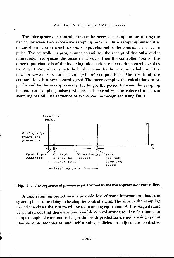
The microprocessor controller makesthe necessary computations during the period between two successive sampling instants. By a sampling instant it is meant the instant at which a certain input channel of the controller receives a pulse. The controller is programmed to wait for the receipt of this pulse and it immediately recognizes the pulse rising edge. Then the controller "reads" the other input channels of the incoming information, delivers the control signal to the output port, where it is to be held constant by the zero order hold, and the microprocessor sets for a ·new cycle of computations. The result of the computations is a new control signal. The more complex the calculations to be performed by the microprocessor, the longer the period between the sampling instants (or sampling pulses) will be. This period will be referred to as the sampling period. The sequence of events can be recognized using Fig. 1.

Sampling pulse

Rising edge:~ ~ ~ Start the procedure

---+L++------11 ~I ~)>

Read inpu:Y ~:ntrol "'Co=at$Wait t channels signal to period for new

l output port _j sampling

pulse ~sampling period

Fig. 1 : The sequence of processes performed by the microprocessor controller.

A long sampling period means possible loss of some information about the system plus a time delay in issuing the control signal. The shorter the sampling period the closer the system will be to an analog equivalent. At this stage it must be pointed out thaJ there are two possible control strategies. The first one is to adopt a sophisticated control algorithm with predicting elements using system identification techniques and self-tunning policies to adjust the controller

-287-

I


parameters to compensate for varying operating conditions of the whole system. In this case there is a long sampling period but the " accurately calculated " control signal which will be issued and hence held constant over the following sampling period will take care ofthe possibly lost information. The second control strategy is to use a simple control algorithm which needs a very short period to be executed. The issued control signal will be accurate enough to work the system during the following short sampling period.

In an electrical power system the frequency is 50 Hz (or 60 Hz in North American systems). The transient time constant of the generators in such systems range between 2 to 6 complete cycles [1 J. It has been found that a sampling time of 10 to 20 ms, i.e. the time of half a cycle to one complete cycle in 50 Hz systems, is most convenient for the proper tracking of the controlled system [2). Such a sampling rate is well above the Nyquist sampling rate. A simple but efficient control algorithm with constant assigned weighting parameters, or even with other computations to vary them on line according to a certain strategy can fit in the required sampling period.

2. THE PHYSICAL MODEL

2.1 The System Under Study

A simple power system has been chosen for this study~ The system under consideration is shown in Fig. 2. This system includes the main components of the power sytem and it is very convenient to study the effects of the A VR in both transient and dynamic performance conditions of the synchronous machine. The synchronous generator in the system resembles a large turbo-alternator with its excitation system represented in the figure as well. The synchronous generator feeds a local load at its terminals and delivers power to a large network through two parallel short transmission lines. The power system is equipped with the necessary switchgear which enables an operator to perform any required changes in the system configuration. The automatic voltage regulator as a two-input singleoutput system is also shown in Fig. 2.

-288-

M.A.L. Badr, M.B. Eteiba, and A.M.O. EI-Zawawi

Excitation

system

Excitation control signal

Transmission line 1

Transmission line 2

Local load

Fig. 2 : The System Under Study.

2.2 The Synchronous Generator and Excitation System

Large system.

bus

The test machine is a three-phase, 3-kVA, 220-V, 60-Hz, 1800-r.p.m. microalternator which has a special design to simulate large synchronous machines [3]. The parameters of this machine are quite close to those of a 590 MVA two-pole turbo alternator except for the open-circuit time constant (T ~0 ). According to the unavoidable limitations of the small size of the micro-alternator its open-circuit time constant is 0.173 seconds, while the same time constant has a value of 4.2 seconds in the large alternator [4]. Therefore the model machine (micro-alternator) has equipped with a shadow winding in the rotor slots and an electronic time-constant regulator (TCR) connected to it. It is the function of the TCR to introduce a negative resistance into the field winding to cancel its active resistance and add a prescribed resistance to develop the required time constant. This TCR can be used to adjust the transient time constant T ~o at any value over the range from 0.5 to 10 seconds. It is through this time constant regulator that T ~o was set to 4.1 s throughout the test [5]. The machine parameters are listed in Appendix I.

-289-


The excitation system applied to the micro-machine and used throughout the

test belongs to the family of solid-state excitation systems with extremely low

time constants [4]. In fact the TCR circuitry serves this purpose too. In addition

to the main function of the TCR of adjusting the time constant T ;o , it acts as

controlled amplifier for the introduction of the excitation voltage (30-45 V de)

from a constant voltage source to the excitation windings of the synchronous

machine rotor [5].

2.3 The Transmission Lines and Local Load

The two transmission lines which link the synchronous generator to the large

system bus are represented in the laboratory model by their resistances and

inductances. One line is permanently connected while the second line undergoes

a series of switching processes in the course of testing the machine under heavy

transients. A ROM-based circuit has been designed and built to perform the required sequences of events on this transmission line. The circuit is described

in reference [6]. The circuit has been used to simulate the case of symmetrical

short circuit at the mid-point of the line with fault clearing process, and either

one of the two cases of successful or unsucessful reclosures and a final tripping of the line in the latter case. The line impedance is .01 + j.3 pu. The local load

impedance is .2 + j.15 pu.

2.4 The Digital Controller

2.4.1 Configuration of the A VR

It has been pointed out that there are two input signals to the A VR. The main

feedback signal is proportional to the machine terminal voltage (VJ The second

signal denoted as the stabilizing signal is proportional to the first derivative of the power angle.

The main feedback signal is obtained by reducing and rectifying the terminal

voltage Vt to obtain a de signal Kv Vt, where Kv is a constant. This signal is compared to a constant reference voltage signal which is related to the bus

reference voltage V R by the same proportionality factor Kv. The error signal is given by

-290-


This signal is introduced to the digit~} controller as shown in Fig. 3

DAVR Excitation system ~ de voltage Control Program

A f v, K.,V,. AV

~-----\,./- D Execution Control 0 K".,w. ~

A of. 1- TCR Exciter - Generator s weights algorithm p rr- r-ow -

K .. v. Kw

Kw

Kv

Fig. 3 : The System Configuration.

The stabilizing signal i> is obtained from a signal proportional to the machine speed. If the actual rotor speed is denoted by w, and the synchronous speed is

a constant equal to w •' then . 8 = k (w- w.).

where k is a constant [1]. This B is directly proportional to the deviation of the rotor speed (~ w) from the synchronous speed and may be represented as

where ~ ~s a. constant. The rotor speed w can be represented by the voltage output sigrlal of a de tacho-generator mounted on the synchronous machine shaft. The speed reference voltage signal is related to the synchronous speed by the same proportionality factor.

The two error signals ~ V and ~ w are used in the digital controller to produce

the input signal y n' where,

and P1 and P2 are the weighting coefficients.

-291-


Reference to Fig. 3 shows that the DA VR can be programmed to perform four distinct functions as represented by the four internal blocks within the DA VR itself. The first block represents the data acquisition system (DAS), which re,ceives the input data, reads them in a strict succession, and stores them in the RAM at certain locations. The last block represents the signal output device. The two other functions of the DA VR are to prepare the required values of the weights P 1 and P 2, and finally to compute the control signal U". These functions are

performed by the control program as indicated in Fig. 3.

2.4.2 The weighing coefficients

The weighting coefficients P 1 and P 2 can be selected in advance according to mode of operation of the generator and the expected dynamic variations and stored in the memory. In this case there is no on-line computation ofthe weights. The function of that part of the DA VR program concerned with the weighting coefficients reduces to fetching those constants from the memory, multiplying them by the corresponding errors, and adding to prepare the input value Y" for the control algorithm.

The second method for dealing with weighting of the input is by dynamically varying them according to the variances of the error signals as described in Appendix II. In this approach the two error signals D. V and D. w are used by the first part of the control program to determine their variances and hence the weighting coefficients P 1 and P 2• Dynamic variation of the weighting coefficients

is extremely useful in forming the control signal at successive instants during the transient period. For example, a sudden short circuit at a point on one transmission line remote from the generator bus will cause the machine terminal voltage to experience a large drop immediately after the occurrence of the short circuit, while the rate of change of the angle is still small. Here, a heavier weight must be given to the voltage error part of the control signal. At another instant, e.g. after the fault is cleared, the terminal voltage builds up quickly, while tlw rotor speed is far from its rated value. Here, the error in speed should rPCPiVP the heavier weight in forming the control signal. This policy enables thP DAVR to operate effectively over a prolonged period of time with a fastPr rPsponsP to put the system back to steady state.

-292-

M.A.L. Badr, M.D. Eteiba, and A.M.O. El-Zawawi

A third method for the calculation of the weighting coefficients has hP<'n suggested and realized by implementing a new subroutine in the control program. The calculation of the j-th weighting coefficient is performed according to the relationship

where, P jo is a fixed weight assigned to the j-th feedback control signal, and Pin is the updated, dynamically varied weight. The main routine for the calculation of Pin is the same for the computation of Pi in the second method with varying weighting coefficients as presented in Appedix II. The main difference in the

implementation is that Pi (t) of equation (3) is replaced by Pin with wi of the same equation assigned another set of values. Equations (1) and (2) still hold correct in the new version. The pre-selected parts of the weights are meant to provide persistent damping effects during dynamic changes in the system, while the dynamically varying parts of the weights provide the fast tracking and compensation during a transient condition.

2.4.3 The control algorithm

A simple but effective proposrtional-plus-integral-plus-derivative (PID) control strategy has been adopted. The PID algorithm routine is executed to obtain the AVR output signal. This algorithm.is described briefly in Appendix III. The set of the controller parameters K1, T1, T. were assigned the values given in reference [8], namely 1, 4 ms, 5 ms, respectively. These PID controller parameters are sele,cted according to the simulation results of reference [7] with some fine adjustment.

2.4.4 The microprocessor implementation

The control program was written in the Assembly language for a MOTOROLA M6800 microprocessor. The processor was equipped with analog to digital converters (ADC) and a data acquisition system (DAS) at the input, and a digital to analog converter at its output. The input signals occupy only three channels out of the eight channels of the DAC. Two signals were conveyed from the power system feedback circuits (for voltage and speed). The third channel was supplied

-293-


from an adjustable frequency pulse generator. A pulse denotes the start of data acquisition to the microprocessor. Although this timing function could have been

performed using software by making a count on the microprocessor, it has been

decided to use an external source to avoid adding a new calculation burden on the microprocessor.

The processor was also equipped with a digital to analog converter (DAC).

Only one of the available four channels was utilized to deliver the output control

signal to the excitation system of the generator.

The control program was written in the form of a short executive main body

and a number of subroutines. The flow chart of the control program is shown in

Fig. 4. The program was used for the three described methods of choosing P 1

and P.2•

In each case the Computation block has different contents. In the first case,

the constant weights P1 , P 2 were directly assigned to their memory

locations. In the second case the dynamically varying weighting coefficients were

computed according to the logic described in Appendix II. In the third case, the

dynamically varying coefficients with constant parts were computed according to the logic described in section 2.4.2.

In the last two cases with varying weights, reffering to equation (6), Vi(t) was

determined using the sum of the squares of errors over the finite period of 16 samples. A 16 element array for each error is formed in the memory to contain the squares of the errors. This number has been selected as a compromise,

between the requirement of sufficient period over which Vi (t) is computed, limited memory size, and computation time for updating the arrays elements every sampling period.

3. TESTS AND RESULTS

The digital voltage regulator with PID controller has been tested together

with each one of the decribed methods of evaluating the relative weights of the

fePdhack signals. Tests were performed for both transient and dynamic modes of operation of the synchronous generator.

-294-


Update PID Controller Variables

Update Error Signals by Reading 1/0 Ports

Yes

Computations

Difference 6. V , 6. w

P1 ' P2: (a) Constant, (b) Dynamically changing, or (c) Dynamically changing with

Constant Parts

Control Signal Yn = 6. V P1 + 6.w P2

Control Program PID Algorithm

Yes

No

Fig. 4 : Flow-chart of the Control Program.

-295-


3.1 Steady State Verification

A common source of trouble with digital regulators is the error which results from rounding-up, and truncation of the manipulated numerical values due to the microprocessor limitations in word size and speed. Accumulation of error has been eliminated in the programming procedure. An accumulated error leads to irregularities in the performance of the system, ultimately leading to issue an erratic control signal. One way of testing a digital controller to check its regular operation and make sure that the unavoidable computational errors do not affect the system performance is to let the system work for a fairly long time without sharp disturbances. The system must be left to operate under a steady state condition only subject to normal dynamic perturbations. The experimental system has been tested in this way.

In this test the power system has been synchronized to the large system bus and adjusted to supply 0.6 of its full-load capacity at 0.75 lagging power factor and left to operate continuously for about 10 hours for each one of the tested methods of weighting coefficients calculations. The operation of the system has been regular all through the whole period. No processing, or calculation of values were detected.

3.2 Dynamic and Transient Tests

The performance of the synchronous generator in response to the following disturbances was recorded:

(a) a sudden change in the mechanical power, (b) a sudden increase in the local load, (c) a sudden rejection of the local load,

(d) a three phase sudden short circuit on one line, tripping off of the faulty line and a successful automatic reclosure of the line.

(e) &three phase sudden short circuit on one line, tripping off of the faulty line, an automatic reclosure of the line while the fault is still there, and a second and final tripping off of the line.

-296-


Each one of these disturbances was applied to the system using the appropriate device. The main purpose of these investigations was to study the stability and dynamic performance of the generator with the DA VR. The power angle was the main performance variable to be recorded.

Results obtained with the digital A VR are compared with those obtained using

a conventional analog AVR having a transfer function KA/(1 + TAS), where KA = 20, and T A was small with respect to the time lags in the field system. The same voltage and speed transducers were used in both the digital and analog regulators.

In the first set of experiments on the system, a careful recording of the control signal as measured at the output port of the digital controller (as delivered to the excitation system) has been performed-for the two severe cases of transients. These are the three phase short-circuit cases with sucessful and unsuccessful reclosures. The records of the control signals are shown in Fig. 5 and Fig. 6 for the successful and unsuccessful reclosures, respectively. The oscillograms show the discrete nature with the zero-order hold effect of the DA VR .. Moreover, the control signals reach their ceiling in the two cases during the periods with low voltage at the generator terminals due to line short circuits. It is for this reason, that the control signal saturates once in Fig. 5 and twice in Fig. 6.

j_ 2V

0 1 2 3 4 5 sec.

Fig. 5 The Output Signal from the DA VR in Response to a Three-phase Short Circuit and Successful Automatic Reclosure. (Constant weighting Coefficients)

-297-


~~~~~~~~~==~==~==~==~t

0 1 2 3 4 sec.

Fig. 6 : DA VR Response to a Three-phase Short Circuit

and Unsuccessful Automatic Reclosure.

(Constant Weighting Coefficeints)

Figure 7 shows the oscillograms of the machine response due to four types of disturbance. At this stage the control program was executed with constant values for P 1 and P

2 •

..l. Control signal SV

"' .J:.. Machine current 2A

--;;r __±_

Power angle 8.9°

~ __:t.

Terminal voltage SOOV

T

--~-L~--J--4--J--+--~-L--~-L--~~ t 0 2 4 6 8 10· sec.

(a) 0.5 kW sudden increase in the mechanical power from half-load.

-298-


j_ Control signal 5V

'";f."'

i Powerangle 18.5°

T i

Armature current 2A T j_

Terminal voltage 400V

T

0 2 4 6 8 10

(b) 25% step increase in the local load. Initial load is 0.85 kW at 0.75 lagging power factor.

i Control signal 5V

T i

Power angle 8.9° T .:l

Armature current 1 OA

-:.y: .t.

-Terminal voltage 800V ~

0 1 2 3 4 5 t sec.

(c) Three-phase short circuit with successful automatic reclosure.

-299-


i Control signal SV

T j_

Power angle 8.9°

'" ±.. Armature current lOA

r ..t...

Terminal voltage 800V

4

0 1 2 3 4 5 t

sec.

(d) Three-phase short circuit with unsuccessful automatic reclosure.

Fig. 7 : Constant Weighting Coefficients DAVR.

Generator Response to System Disturbances.

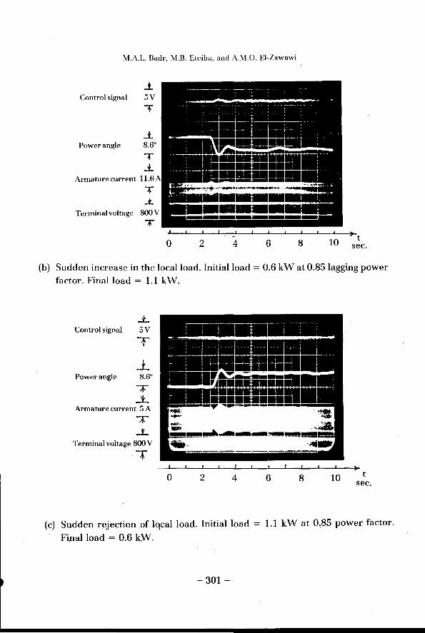
The response of the generator when the DA VR was programmed to vary the

weighting coefficient dynamically is represented by the oacillograms of Fig. 8.

The response curves show a general effect of lower first overshoot but a more oscillatory response.

\ Control signal sv

T

.L Power angle 8.6°

r ...L

Armature current 12 A r ..t..

Terminal voltage 800 V T

0 2 4 6 8 10 t sec.

(a) Suddel). increase in the mechanical power. Initial load = 0.6 kW at 0.8lagging power factor. Final load= 1.1 kW.

-300-


.i Control signal 5 V

Power angle

,.. ...i._

T ..i.

Armature current 11.6

Terminal voltage

T ..t.

0 2 4 6 8 10 t sec.

(b) Sudden increase in the local load. Initial load= 0.6 kW at 0.85lagging power

factor. Final load= 1.1 kW .

..t.. Control signal 5 V

T

Power angle 8.6°

T _1..

Armature current 5 A

T J....

Terminal voltage 800 V

T

0 2 4 6 8 10 t sec.

(c) Sudden rejection of lqcal load. Initial load = 1.1 kW at 0,85 power factor.

Final load = 0.6 kW.

-301-


Powerangle 8.6°

T

Armature j_ current SA

T

0 1 2 3 4 sec.

(d) Three-phase short circuit with successful automatic reclosure.

Power angle 8.6°

T

Armature L current SA

T

0 2 4 6 8 10 t sec.

(e) Three-phase short circusit with unsuccessful automatic reclosure.

Fig. 8 DA VR with Dynamically changing weighting Coefficients. Generator response to system distrubances.

-302-


Test results of the experimental system with the DAVR programmed according

to the third method are shown in Fig. 9. It can be noted that the variation of a·

part of each one of the weighting coefficients reduces the first overshoot as well

as to give a better damping to the system.

Power angle 8.6°

T

Armature _L current SA

T 0 2 4 6 8 10 't

sec.

(a) Step change in mechanical load. Initial load ""' 0.35 kW at 0.9 lagging power

factor. Final load = 0.85 kW.

Powerangle 18.5°

T

Armature j_ current 2A

T 1

•• II fiMtM! 1 ,.. 0 2 4 6 8 10 t

sec.

(b) 25% step increase in local load. Initial load =0.85 kW at 0.85lagging power

factor.

-303-


..L Control signal 5 V

T

..L Powerangle 18.5°

T ..:L


I: Terminal voltage 800 V

T

0 2 4 6 8 10

(c) 3-phase short circuit with successful automatic reclosure.

_L Control signal 5 V

T

j_ Power angle 8.6°

T L


I: Terminal voltage 800 V

T 6 8 10

t sec.

t sec.

(d) 3-phase short circuit with unsuccessful automatic reclosure.

Fig. 9 DA VR with constant-part dynamically changing weighting coefficients. Generator response to system disturbances.

-304-


For comparison with an analog A VR, the case of short circuit at the middle of one transmission line, fault clearing and successful automatic reclosure of the line has been tested on the system with an analog A VR connected in the place of the DA VR. The A VR has the same main feedback and stabilizing signals as the DAVR. The analog A VR was built using operational amplifiers and its output has been delivered to the control circuit of the excitation system as in the case with the control DA VR. Figure 10 shows that the analog A VR provides a heavily oscillating response with a maximum first overshoot in the power angle.

No digital Control signal

l_ Powerangle 8.9°

T _l_


I Terminal voltage 800 V

T 0 2 4 6 8 10 t

sec.

Fig. 10 Generator response to a 3-phase short circuit and successful automatic

reclosure with analog A VR.

4. DISCUSSION

4.1 Discussion of Results

Referring to the test results it can be deduced that the variation of the whole weighting coefficients improves the system stability by controlling the magnitude of the power angle in the first swing. On the other hand, it seems to take the

-305-


system a slightly longer period to damp out the oscillation. The simple PID algorithm with constant weghting coefficients provides a slightly larger angle overshoot but better damping.

The third method with varying weighting coefficients which have constant offset values have been noticed to be most effective. Both short settling times and limited first angle overshoots have been gained by using this technique.

The use of a more effective programming technique and a faster microprocessor will certainly reduce the sampling period and improve the response of the system to both dynamic and transient disturbances.

4.2 Relevance of Results to 50-Hz Power Systems

Traditionally, electrical power systems are classified as 50-Hz or 60-Hz systems, according to their nominal frequencies. 50-Hz systems are common in

many parts of the world including Gulf area (except some sub-systems in Saudi Arabia), while 60-Hz systems are characteristic for North America. The voltage levels of generation, transmission, and distribution of electrical energy, however remain about the same in all systems. Standard generation voltages ranging from

3.3 kV are common in both 50-Hz and 60-Hz systems. In addition, standard transmission and distribution voltages of 380, 220, 66, 33, 11, ... k V are common in both systems.

The tests described in the present paper have been carried out on a 60-Hz power system. The sampling time was chosen to be 16 ms, which is slightly less than a complete perriod of the power frequency. When such techniques are to be applied to a 50-Hz system as the Qatar Electric System (QES), a close performance is expected to occur. The same sampling period may be used or it can be even increased to 20 ms without loosing accuracy in the system results. Here, 20 ms is the periodical time of the 50-Hz frequency. Reffering to the discussion on sampling rates included in the intoduction of the present paper (paragraph 2), the necessary calculations can be done with an extra remainder during each sampling cycles.

-306-

M.A.L. Badr. M.B. Eteiba. and A.M.O. El-Zawawi

4.3 Influence of Variations in Speed and the Type of Prime-Mover on Results

Speed changes of the generating unit are continuously monitored and constitute the second feed back signal to the DA VR in the proposed ·~ystem. Therefore, the DA VR takes these changes into consideration when computing the control signal each sampling period. In dynamic performance, variation of speed is thus automatically accounted for irrespective of the type of the primemover of the synchronous generator.

In cases of transient performances following system faults or heavy switching conditions, speed variations which take place after the termination of the electromagnetic process have been neglected in the present investigation on control algorithms of DA VR systems. This is because the electromagnetic phenomena handled by the A VR is much faster than electromechanical process associated with variations in unit speeds. The order of the time-constant associated with the electromagnetic transient performance does not exceed the period of 20 complete cycles, i.e. 400 ms in a 50-Hz system, while the mechanical time constants of the generating units vary from few seconds to more than 10 seconds in large alternators [4]. The higher·values refer to hydro-turbine units,

the middle range corresponds to large steam-turbine units, while the lower range belongs to small steam-turbine and gas-turbine units.

It may be noted that the DA VR with sampling period of 20 ms is suitable for application with gas turbine driven generators which are common in QES.

5. CONCLUSIONS

The test results obtained from the physical model ofthe studied pow~r system show that the digital PID DAVR is quite effective under various system disturbances. Tests over fairly long continuous periods did not show any drift or instability problem.

The use of three algorithms of the DAVR to perform on-line control of the system has proven that a PID digital controller with a partially vari~le weighting coefficients of the main and stabilizing signals is most effective in limiting the system swinging and also provides faster settling.

-307-


REFERENCES

1. E.W. Kimbark. "Power System Stability, Vol. 3, Synchronous Machines." J. Wiley & Sons, 1964.

2. O.P. Malik, G.S. Hope, M.A.L. Badr, P. Walsh, and G. Hancock. "Implementation and Test Results

of a Microprocessor-based Voltage Regulator." The Bulletin of the Canandian Papers Presented

to the Tenth Pan-American Congress of Mechanical, Electrical and Allied Engineering Branches, COPIMERA 84, Buenos-Aires, Argentina, October 1984, Paper No. 5.

3. T.J. Hammos, and A.J. Parsons. "Design of Microalternator fo.r Power-System Stability Investigation." Proc. lEE, Vol. 118, 1971, pp. 1421-1441.

4. P.M. Anderson and A.A. Fouad. "Power System Control and Stability, Vol. 1." The Iowa State University Press, 1977.

5. M.A.L. Badr and Kh.I. Saleh. "Control of Micro-Alternator Transient Characteristics by a Time

Constant Regulator." The Bulletin of the Internatinal AMSE 84, Athens Summer Conference on Modeling and Simulation, June 1984, Athens, Greece, pp. 13-23.

6. Kh.I. Saleh and M.A.L. Badr. "ROM-Based Sequential Circuits for Experimental Simulation of Power System Disturbances." Electrical Machines and Power Systems, Vol. 13, No. 1, 1987.

7. M.A.L. Badr, G.S. Hope, and O.P. Malik. "A Self-Tuning PID Voltage Regulator for Synchronous Generators." The Canadian Electrical Engineering Journal, Vol. 8, No. 1, 1983, pp. 18-27.

8. O.P. Malik, G.S. Hope and M.A.L. Badr. "Experimental Results for a Digital PID Voltage Regulator

with Dynamically Changing Weighting Coefficients." The Proceedings of the IFAC Symposium on Power Systems and Power Plant Control", Beijing, PRC, Aug. 12-15, 1986, pp. 381-386.

-308-


APPENDIX I : SYNCHRONOUS MACHINE PARAMETERS

H 4.5s,

X" d 0.233pu,

T' do 4.1 s,

xd X= 2.17pu, q

xl 0.128pu,

T' d 0.626s,

X' d 0.375pu,

r a 0.0047pu,

T" d 0.0225s.

APPENDIX II : DYNAMIC VARIATION OF THE WEIGHTING COEFFICIENTS

The synchronous generator and its excitation system can be described as a single-input multi-output controlled process so far as the A VR is concerned. The

input is the control signal produced by the A VR and the outputs are the terminal voltage, rotor speed, rotor angle, active power, ... etc. A combination of the weighted deviations from reference values of some of the output signals are used by the controller (A VR) to generate the control signal as shown in Fig. 11. The control objective is to minimize, as nearly as possible, the deviation of each

individual weighted output.

!disturbance Output sig

uw CONTROLLED PROCESS .. (Generator and Exciter)

H Pd J

Controller y(t) ::2. P3 C3 (t) ~ ....... L...-- (AVR) j:l

. lr:?-1 [l P-3 I

Fig. 11 : Dynamic Variation of Weighting Coefficients.

-309-

nals c,(tJ

C.,(t)


The controller input signal, y(t), is defined as:

J y(t) = l Pj cj (t) (1)

.j=l

where j is the assigned weisght for the j-th output deviation Ci (t), and J is the total number of the weighted outputs.

The choice of the weighting coeffcients Pi is important and is generally made such that:

1 and 0:::::; P.:::::; 1, J (2)

are satisfied. These conditions mean that only the relative values of Pi need to be selected. Normally, the relative values of the weights Pi are assigned according to the physical structure of the system. The outputs which required to be closer to their reference values are weighted more heavily. If the system is disturbed, some variables will move far from their desired values while others will stay close. If the weighting coefficients are constant, the system performance will deteriorate.

The proposed criterion is to vary the weights dynamically with variances of the corresponding ourput signals (8]. Te variances of the control process output signals are computed from the deviations of these signals from their reference values using the relationship:

(3)

where wi are prescribed constants which in fact represent the initial values of the weights, Vi (t) are the variances of the outputs Ci' and V(t) is defined by:

J V(t) = I wj vi (t).

j=l

-310-


The procedure of dynamic variation of the weighting coefficients can be

described in the following steps:

(i) At each sampling instant, when the terminal volatage and rotor speed

are read, variances of these qualities are computed as:

t

I C/(t) v (t) = - 1--

j N+1 (4)

i=t-N

where, N is a finite observation interval expressed in number of sampling periods.

(ii) The new weights are computed using equation (3). This procedure satisfies

equation (2).

APPENDIX III : PID CONTRROILER ALGORITHM

The algorithm of a PID controller, shown in Fig. 12(a), is given by:

(5)

In Laplace transform, equation (5) takes the form:

u 1 -- = K (1+--+TS) y p TS D !

(6)

where T1

is called the integral time and is equal to Kn I Kr. This form of the PID algorithm is called "ideal" or "noninteractive". Most controllers however have

a transfer function more nearly represented by:

u (7) y

where:

T d equivalent of integral time, T d equivalent of derivative time,

~ = a constant equal toT /1' 2

Tr = time constant of filter.

-311-


This form is callled the "real" or "interactive" PID algorithm [8]. In actual practice, the ideal form is further modified by a filter which pmltilpies the right

hand of equation (6). Some algebraic manipulation gives the equavalents:

K" = K1 (T1 + T2)/1\ Tr = Tt + T2

TD = TlT/(Tl + T2) } (8)

The real algorith makes the controller less sensitive to shifts in the system parameters.

From equation (7), the real form of the PID algorithm is represented by:

y T2S + 1 1 TrS + 1 . K (1 + -T S )

l u (9)

This form permits the control equation to be implemented in blocks as shown in Fig. 12(b) [7]. Equation (9) is discretized for implementation on the

microprocessor. Discrete forms of the individual blocks are given in Reference [7].

R y u

c

Fig. 12(a) : "Ideal" PID Cont':oller.

Derivative Gain

y T~s + 1 D J K~ l u + ~ T.,.s + 1 I I

+ Integral

K~ I -T~s

Fig. 12(b) : "Real" PID Algorithm.

-312-

\

control algorithms of digital automatic voltage regulators

Documents