control and numerics: continuous versus discrete approaches · control and numerics: continuous...

Control and numerics: Continuous versus discreteapproaches

Enrique Zuazua

Ikerbasque & Basque Center for Applied Mathematics (BCAM)Bilbao, Basque Country, Spain

[email protected]

http://www.bcamath.org/zuazua/

LJLL, February 2012Joint work with S. Ervedoza and A. Marica

Enrique Zuazua (BCAM) Control and numerics LJLL 1 / 61

Motivation

Table of Contents

1 Motivation

2 The control of wavesWhy?A toy modelThe discrete approachA remedy: Fourier filtering

3 The multi-dimensional case

4 Heterogeneous grids

5 Conclusions and Perspectives


Motivation

Motivation

Control problems for PDE are important for at least two reasons:

They emerge in most real applications:

PDE as the models of Continuum and Quantum Mechanics.

Control and/or Optimization as essential step in allprocesses.

They demand a better master of the standard PDE models andnew analytical tools.

This need of new analytical tools is enhanced when facing numericalsimulation problems!

Furthermore, these kind of techniques are of application in some otherfields, such as inverse problems, optimal shape design and parameteridentification problems.


Motivation

Topics to be addressed:

1 The wave equation: propagation of discrete waves

2 Heterogenous grids

3 Perspectives


The control of waves

Table of Contents

1 Motivation






The control of waves Why?

Outline

1 Motivation






The control of waves Why?

http://www.ind.rwth-aachen.de/research/noise reduction.html


The control of waves A toy model

Outline

1 Motivation







Control of 1− d vibrations of a string

The 1-d wave equation, with Dirichlet boundary conditions, describing thevibrations of a flexible string, with control on one end:

ytt − yxx = 0, 0 < x < 1, 0 < t < Ty(0, t) = 0; y(1, t) =v(t), 0 < t < Ty(x , 0) = y 0(x), yt(x , 0) = y 1(x), 0 < x < 1

y = y(x , t) is the state and v = v(t) is the control.The goal is to stop the vibrations, i.e. to drive the solution to equilibriumin a given time T : Given initial data y 0(x), y 1(x) to find a controlv = v(t) such that

y(x ,T ) = yt(x ,T ) = 0, 0 < x < 1.



The dual observation problem

The control problem above is equivalent to the following one, on theadjoint wave equation:

ϕtt − ϕxx = 0, 0 < x < 1, 0 < t < Tϕ(0, t) = ϕ(1, t) = 0, 0 < t < Tϕ(x , 0) = ϕ0(x), ϕt(x , 0) = ϕ1(x), 0 < x < 1.

The energy of solutions is conserved in time, i.e.

E (t) =1

2

∫ 1

0

[|ϕx(x , t)|2 + |ϕt(x , t)|2

]dx = E (0), ∀0 ≤ t ≤ T .

The question is then reduced to analyze whether the folllowing inequalityis true. This is the so called observability inequality:

E (0) ≤ C (T )

∫ T

0|ϕx(1, t)|2 dt.



The answer to this question is easy to gues: The observability inequalityholds if and only if T ≥ 2.

E(0) ≤ T

0|ϕx(1, t)|2dt

Wave localized at t = 0 near the extreme x = 1 that propagates withvelocity one to the left, bounces on the boundary point x = 0 and reachesthe point of observation x = 1 in a time of the order of 2.



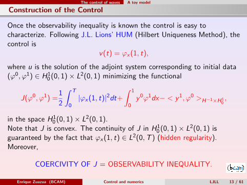
Construction of the Control

Once the observability inequality is known the control is easy tocharacterize. Following J.L. Lions’ HUM (Hilbert Uniqueness Method), thecontrol is

v(t) = ϕx(1, t),

where u is the solution of the adjoint system corresponding to initial data(ϕ0, ϕ1) ∈ H1

0 (0, 1)× L2(0, 1) minimizing the functional

J(ϕ0, ϕ1) =1

2

∫ T

0|ϕx(1, t)|2dt+

∫ 1

0y 0ϕ1dx− < y 1, ϕ0 >H−1×H1

0,

in the space H10 (0, 1)× L2(0, 1).

Note that J is convex. The continuity of J in H10 (0, 1)× L2(0, 1) is

guaranteed by the fact that ϕx(1, t) ∈ L2(0,T ) (hidden regularity).Moreover,

COERCIVITY OF J = OBSERVABILITY INEQUALITY.



The continuous numerical approach: Gradient algorithms

The control was characterized as being the minimizer overH1

0 (0, 1)× L2(0, 1) of

J(ϕ0, ϕ1) =1

2

∫ T

0|ϕx(1, t)|2dt+

∫ 1

0y 0ϕ1dx− < y 1, ϕ0 >H−1×H1

0.

We produce an algorithm in which:

We apply a gradient iteration algorithm to J.This leads to an iterative process

(ϕ0k , ϕ

1k), k ≥ 1

so that∂xϕk(1, t) = vk(t)→ v(t), as k →∞.

We replace J by some numerical approximation Jh with an order hθ,and apply a discrete version of the iterative process above to buildapproximations of vk .



Note however that computing gradients, in practice, may be hard.



Classical steepest descent:

J : H → R. Two main assumptions:

< ∇J(u)−∇J(v), u− v >≥ α|u− v |2, |∇J(u)−∇J(v)|2 ≤ M|u− v |2.

Then, foruk+1 = uk − ρ∇J(uk),

we have|uk − u∗| ≤ (1− 2ρα + ρ2M)k/2|u1 − u∗|.

Convergence is guaranteed for 0 < ρ < 1 small enough (ρ < α/M).

Compare with the continuous marching gradient system

u′(τ) = −∇J(u(τ)).



The following holds:

Theorem

(S. Ervedoza & E. Z., 2011)In

K ∼ C | log(h)|iterations, the controls vK

h obtained after applying K iterations of thegradient algorithm to Jh fulfill:

||v − vKh || ≤ C | log(h)|max(θ,1)hθ.

Note that for the classical Finite Difference and Finite Element methodsfor the wave equation the convergence order is θ = 2/3.

We have developed the continuous program successfully!



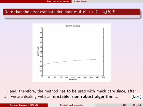
Note that the error estimate deteriorates if K >> C | log(h)|!!!

0 50 100 150 200 250 300 350 400 450 5000

0.1

0.2

0.3

0.4

0.5

0.6

0.7

0.8

0.9

1

Iterations

Rel

ativ

e Er

ror

Error Vs Iterations

... and, therefore, the method has to be used with much care since, afterall, we are dealing with an unstable, non-robust algorithm....



Convergence of the descent algorithm for the continuous model and theconvergence of the numerical scheme in the classical sense of numericalanalysis leads to:

||v − vkh || ≤ ||v − vk ||+ ||vk − vk

h || ≤ C [σ(ρ)k + khθ].

Note that, in here, nothing has been used about the actual properties ofcontrol of the numerical scheme.

The estimate deteriorates when khθ >> σ(ρ)k .



The continuous method can not be implemented, in a reliable manner, asone would expect/wish: To apply a descent or iterative algorithm for adiscrete functional Jh, without worrying about possible divergence of theprocess beyond a certain threshold of iterations.

The same occurs to other methods, based on different iterative algorithmsfor building continuous controls, as for instance, the one developed by N.Cindea et al.1 based on D. Russell’s2 method of “stabilization impliescontrol”, also closely related to the works by Auroux and Blum on thenudging method for data assimilation for Burgers like equations.

1N. Cindea, S. Micu & M. Tucsnak, An approximation method for exact controls ofvibrating systems. SICON, 49 (3), (2011), 1283–1305.

2D. Russell, Controllability and stabilizability theory for linear partial differentialequations: Recent progress and open questions, SIAM Rev., 20 (1978), 639–739.


The control of waves The discrete approach

Outline

1 Motivation







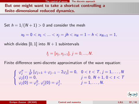
But one might want to take a shortcut controlling afinite-dimensional reduced dynamics.

Set h = 1/(N + 1) > 0 and consider the mesh

x0 = 0 < x1 < ... < xj = jh < xN = 1− h < xN+1 = 1,

which divides [0, 1] into N + 1 subintervals

Ij = [xj , xj+1], j = 0, ...,N.

Finite difference semi-discrete approximation of the wave equation:

ϕ′′j − 1h2 [ϕj+1 + ϕj−1 − 2ϕj ] = 0, 0 < t < T , j = 1, . . . ,N

ϕj(t) = 0, j = 0, N + 1, 0 < t < Tϕj(0) = ϕ0

j , ϕ′j(0) = ϕ1

j , j = 1, . . . ,N.



From finite-dimensional dynamical systems to infinite-dimensional ones inpurely conservative dynamics.....



Then it should be sufficient to minimize the discrete functional

Jh(ϕ0, ϕ1) =1

2

∫ T

0

|ϕN(1, t)|2h2

dt+hN∑

j=1

ϕ1j y 0

j − hN∑

j=1

ϕ0j y 1

j ,

which is a discrete version of the functional J of the continuous waveequation since

−ϕN(t)

h=ϕN+1 − ϕN(t)

h∼ ϕx(1, t).

Then

vh(t) = −ϕ?N(t)

h.



A NUMERICAL EXPERIMENT

Plot of the initial datum to be controlled for the string occupying thespace interval 0 < x < 1.Plot of the time evolution of the exact control for the wave equation intime T = 4.



The control diverges as h→ 0.



The discrete approach naively or directly applied diverges as well.

In this case our algorithm gets the minimizer of Jh. But the minimizer ofJh is very far form that of J: This is a clear case in which Γ-convergencewith respect to the parameter h→ 0 fails.



WHY?

The Fourier series expansion shows the analogy between continuous anddiscrete dynamics.Discrete solution:

~ϕ =N∑

k=1

ak cos

(√λh

kt

)+

bk√λh

k

sin

(√λh

kt

) ~wh

k .

Continuous solution:

ϕ =∞∑

k=1

(ak cos(kπt) +

bk

kπsin(kπt)

)sin(kπx)



Recall that the discrete spectrum is as follows and converges to thecontinuous one:

λhk =

4

h2sin2

(kπh

2

)

λhk → λk = k2π2, as h→ 0

whk = (wk,1, . . . ,wk,N)T : wk,j = sin(kπjh), k, j = 1, . . . ,N.

The only relevant differences arise at the level of the dispersion propertiesand the group velocity. High frequency waves do not propagate, remaincaptured within the grid, without never reaching the boundary. Thismakes it impossible the uniform boundary control and observation of thediscrete schemes as h→ 0.



Nπ

1 2 3

Discrete problem

Continuous problemλ

k1/2

... N k

Graph of the square roots of the eigenvalues both in the continuous and inthe discrete case. The gap is clearly independent of k in the continuouscase while it is of the order of h for large k in the discrete one.



A numerical phamtom

~ϕ = exp(

i√λN(h) t

)~wN − exp

(i√λN−1(h) t

)~wN−1.

Spurious semi-discrete wave combining the last two eigenfrequencies withvery little gap:

√λN(h)−

√λN−1(h) ∼ h.

h = 1/61, (N = 60), 0 ≤ t ≤ 120.Enrique Zuazua (BCAM) Control and numerics LJLL 31 / 61

The control of waves A remedy: Fourier filtering

Outline

1 Motivation







Fourier filtering

Nπ

1 2 3 ... kN

Discrete problem

Continuous problemλ

k1/2

To filter the high frequencies, keeping the components k ≤ δ/h with0 < δ < 1. Then the group velocity remains uniformly bounded below anduniform observation holds in time T (δ) > 2 such that T (δ)→ 2 as δ → 0.



Relaxed controls:

Then, the filtering algorithm can be implemented as follows:

Minimize Jh over the class of filtered solutions with filteringparameter 0 < δ < 1 and T > T (δ);

This yields controls v δh such that

vδh → v as h→ 0;

The corresponding states ~yh satisfiy:

πδ(~yh) ≡ πδ(~yh′) ≡ 0.

This is a relaxed version of the controllability condition.



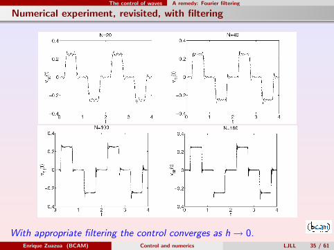
Numerical experiment, revisited, with filtering

With appropriate filtering the control converges as h→ 0.Enrique Zuazua (BCAM) Control and numerics LJLL 35 / 61


The discrete approach when applied directly fails, but it can curedborrowing ideas from the continuous analysis. The bonus is that:

We compute numerical approximations of the controls that performwell, in an identified manner, controlling a Fourier projection ofsolutions at the discrete level.

The algorithm converges is stable and robust, an the error diminishesas the number of iterations →∞.


Multi-dimensions

Table of Contents

1 Motivation






Multi-dimensions

The multi-dimensional case.

Similar results are true in several space dimensions. The region in whichthe observation/control applies needs to be large enough to capture allrays of Geometric Optics. This is the so-called Geometric ControlCondition introduced by Ralston (1982) and Bardos-Lebeau-Rauch (1992).

Let Ω be a bounded domain of Rn, n ≥ 1, with boundary Γ of class C 2.Let Γ0 be an open and non-empty subset of Γ and T > 0.

ytt −∆y = 0 in Q = Ω× (0,T )y =v(x , t)1Γ0 on Σ = Γ× (0,T )(x , 0) = y 0(x), yt(x , 0) = y 1(x) in Ω.


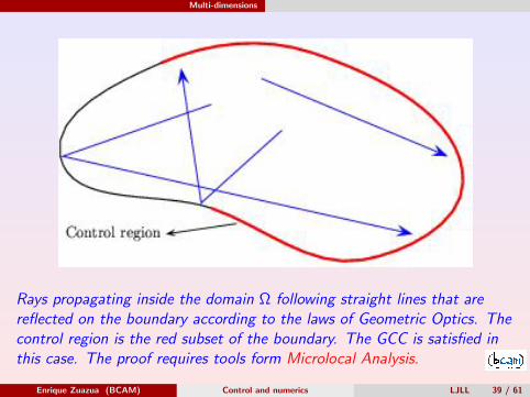
Multi-dimensions

Rays propagating inside the domain Ω following straight lines that arereflected on the boundary according to the laws of Geometric Optics. Thecontrol region is the red subset of the boundary. The GCC is satisfied inthis case. The proof requires tools form Microlocal Analysis.


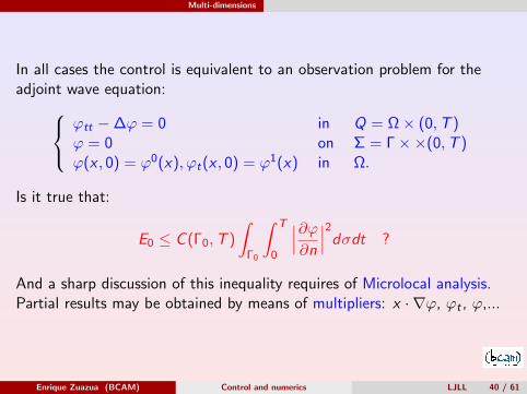
Multi-dimensions

In all cases the control is equivalent to an observation problem for theadjoint wave equation:

ϕtt −∆ϕ = 0 in Q = Ω× (0,T )ϕ = 0 on Σ = Γ××(0,T )ϕ(x , 0) = ϕ0(x), ϕt(x , 0) = ϕ1(x) in Ω.

Is it true that:

E0 ≤ C (Γ0,T )

∫

Γ0

∫ T

0

∣∣∣∂ϕ∂n

∣∣∣2dσdt ?

And a sharp discussion of this inequality requires of Microlocal analysis.Partial results may be obtained by means of multipliers: x · ∇ϕ, ϕt , ϕ,...


Multi-dimensions

THE 5-POINT FINITE-DIFFERENCE SCHEME

ϕ′′j ,k −1

h2[ϕj+1,k + ϕj−1,k − 4ϕj ,k + ϕj ,k+1 + ϕj ,k−1] = 0.

The energy of solutions is constant in time:

Eh(t) =h2

2

N∑

j=0

N∑

k=0

[| ϕ′jk(t) |2

+

∣∣∣∣ϕj+1,k(t)− ϕj ,k(t)

h

∣∣∣∣2

+

∣∣∣∣ϕj ,k+1(t)− ϕj ,k(t)

h

∣∣∣∣2].

Without filtering observability inequalities fail in this case too.Understanding how filtering should be used requires of a microlocalanalysis of the propagation of numerical waves combining von Neumannanalysis and Wigner measures developments (N. Trefethen, P. Gerard, P.L. Lions & Th. Paul, G. Lebeau, F. Macia, ...).


Multi-dimensions

The von Neumann analysis.

Symbol of the semi-discrete system for solutions of wavelength h

ph(ξ, τ) = τ2 − 4(sin2(ξ1/2) + sin2(ξ2/2)

),

versus p(ξ, τ) = τ2 − [|ξ1|2 + |ξ2|2].Both symbols coincide for (ξ1, ξ2) ∼ (0, 0).Solving the bicharacteristic flow we get the discrete rays:

xj(t) = −sin(ξj)

τt + xj ,0, (versus xj(t) = −ξj

τt + xj ,0.)

RAYS ARE STILL STRAIGHT LINES. BUT! The velocity is

|x ′(t)| ≡[∣∣∣∣

sin(ξ1)

τ

∣∣∣∣2

+

∣∣∣∣sin(ξ2)

τ

∣∣∣∣2]1/2

THE VELOCITY OF PROPAGATION VANISHES !!!!!!! in the followingeight points

ξ1 = 0,±π, ξ2 = 0,±π, (ξ1, ξ2) 6= (0, 0).


Multi-dimensions


Multi-dimensions

Controls in multi-d may develop complex and unexpected patterns, in viewof the laws of Geometric Optics.

G. Lebeau and M. Nodet, Experimental Study of the HUM ControlOperator for Linear Waves, Experimental Mathematics, 2010.


Heterogeneous grids

Table of Contents

1 Motivation






Heterogeneous grids

In practice, grids are not uniform and, accordingly, the Fourier and vonNeumann analysis above is not sufficient to describe the propagation ofhigh frequency numerical solutions. A new symbolic calculus is needed todefine the discrete rays.


Heterogeneous grids

Problem formulation

The wave equation with variable coefficients on R:

ρ(y)utt − (σ(y)uy )y = 0, t > 0, y ∈ R. (1)

Energy conserved in time:

Eρ,σ(u0, u1) :=1

2

∫

R

(ρ(y)|ut(y , t)|2 + σ(y)|uy (y , t)|2) dy .


Heterogeneous grids

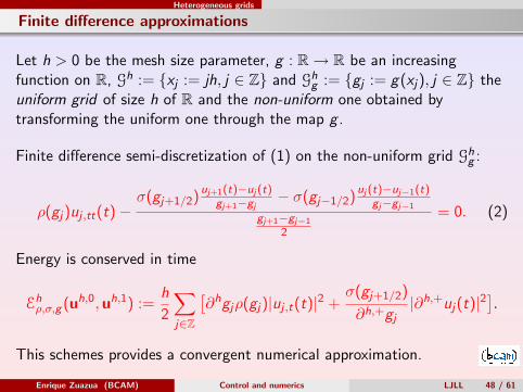
Finite difference approximations

Let h > 0 be the mesh size parameter, g : R→ R be an increasingfunction on R, Gh := xj := jh, j ∈ Z and Gh

g := gj := g(xj), j ∈ Z theuniform grid of size h of R and the non-uniform one obtained bytransforming the uniform one through the map g .

Finite difference semi-discretization of (1) on the non-uniform grid Ghg :

ρ(gj)uj ,tt(t)−σ(gj+1/2)

uj+1(t)−uj (t)gj+1−gj

− σ(gj−1/2)uj (t)−uj−1(t)

gj−gj−1

gj+1−gj−1

2

= 0. (2)

Energy is conserved in time

Ehρ,σ,g (uh,0,uh,1) :=

h

2

∑

j∈Z

[∂hgjρ(gj)|uj ,t(t)|2 +

σ(gj+1/2)

∂h,+gj|∂h,+uj(t)|2

].

This schemes provides a convergent numerical approximation.


Heterogeneous grids

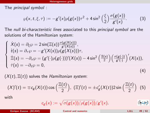
The principal symbol :

℘(x , t, ξ, τ) := −g ′(x)ρ(g(x))τ2 + 4 sin2(ξ

2

)σ(g(x))

g ′(x). (3)

The null bi-characteristic lines associated to this principal symbol are thesolutions of the Hamiltonian system:

X (s) = ∂ξ℘ = 2 sin(Ξ(s))σ(g(X (s)))g ′(X (s)) ,

t(s) = ∂τ℘ = −g ′(X (s))ρ(g(X (s)))τ,

Ξ(s) = −∂x℘ = (g ′(·)ρ(g(·)))′(X (s))− 4 sin2(

Ξ(s)2

)(σ(g(·))g ′(·)

)′(X (s)),

τ(s) = −∂t℘ = 0,(4)

(X (t),Ξ(t)) solves the Hamiltonian system:

(X )′(t) = ∓cg (X (t)) cos(Ξ(t)

2

), (Ξ)′(t) = ±c ′g (X (t))2 sin

(Ξ(t)

2

)(5)

withcg (x) :=

√σ(g(x))/ρ(g(x))/g ′(x).


Heterogeneous grids

Using Wigner transforms, high frequency solutions can be shown topropagate and concentrate along those rays provided cg ∈ C 1,1(R).This means that the coefficients σ and ρ need to be in C 1,1(R) and thegrid transformation g ∈ C 2,1(R).

Gerard, P., Markowich, P., Mauser, N., Poupaud, Ph. Homogenizationlimits and Wigner transforms, Comm. Pure Appl. Math., 1997.

Lions P.-L., Paul, Sur les mesures de Wigner, Rev. MatematicaIberoamericana, 1993.

Macia, F. Wigner measures in the discrete setting: high frequencyanalysis of sampling and reconstruction operators, SIAM J. Math.Anal., 2004.


Heterogeneous grids

Numerical simulations

−1 −0.8 −0.6 −0.4 −0.2 0 0.2 0.4 0.6 0.8 10

0.5

1

1.5

2

2.5

3

3.5

4

4.5

5

1 0.5 0 0.5 10

1

2

3

4

5

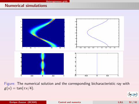
Figure: The numerical solution and the corresponding bicharacteristic ray withg(x) = tan(πx/4).


Heterogeneous grids

1 0.5 0 0.5 10

1

2

3

4

5

−1 −0.5 0 0.5 10

1

2

3

4

5

Figure: The numerical solution and the corresponding bicharacteristic ray withg(x) = 2 sin(πx/6).


Heterogeneous grids

−2 −1 0 1 20

π/2

3π/2

2π

π

−2 −1 0 1 20

π/2

π

3π/2

2π

Figure: The phase portrait for the grid transformations g(x) = tan(πx/4) andg(x)=2sin(πx/6).


Heterogeneous grids

−1 0 1−1

0

1

−1 0 1−1

0

1

Figure: Grid corresponding to the transformations g(x) = tan(πx/4) andg(x) = sin(πx/6) respectively.


Heterogeneous grids


Heterogeneous grids

The analysis above can be extended to the multi-dimensional case,provided grids can be mapped smoothly into uniform grids as in theexample below:


Heterogeneous grids

But there is istill plenty to be done to understand the behavior of discretewaves over very irregular meshes:


Conclusions and Perspectives

Table of Contents

1 Motivation







Conclusions

Efficient and rigorous numerical computation of controllers can bebuilt but often combining tools from the continuous and the discreteapproaches.Heterogeneous grids may lead to novel unexpected phenomena ofdiscrete wave propagation.Plenty is still to be done in the interfaces between PDE, Control,Numerics, Harmonic Analysis,...Similar issues are relevant in many other contexts as well, forinstance, control of conservation laws in the presence of shocks(S. Ulbrich, M. Giles, C. Bardos & O. Pironneau, A. Bressan & A.Marson, E. Godlewski & P. A. Raviart, C. Castro, F. Palacios & E. Z.,...)

This is only one example of the kind of models and problems arisingin the large field of optimal shape design in aeronautics.



Perspectives

Multi-resolution filtering techniques.

Adaptivity.

More singular and heterogeneous grids.

Numerical control of waves in random media and in the presence ofnoise.

Robust controllers.

Multiphysics systems: thermoelasticity, fluid-structure interaction,...

Networks.



Some references:

E. Z. Propagation, observation, and control of waves approximated byfinite difference methods. SIAM Review, 47 (2) (2005), 197-243.

S. Ervedoza and E. Z. The Wave Equation: Control and Numerics, in“Control and stabilization of PDE’s”, P. M. Cannarsa y J. M. Coron,eds., “Lecture Notes in Mathematics”, CIME Subseries, SpringerVerlag, to appear.

L. Ignat and E. Z. Convergence of a multi-grid method for the controlof waves, J. European Math. Soc., 11 (2009), 351-391.

A. Marica and E. Z., Propagation of 1− d waves in regular discreteheterogeneous media: A Wigner measure approach, to appear.


control and numerics: continuous versus discrete approaches · control and numerics: continuous...

Documents