control and optimization of electric ship propulsion
TRANSCRIPT

Control and Optimization of Electric ShipPropulsion Systems with Hybrid Energy Storage
by
Jun Hou
A dissertation submitted in partial fulfillmentof the requirements for the degree of
Doctor of Philosophy(Electrical Engineering: Systems)
in the University of Michigan2017
Doctoral Committee:
Professor Heath Hofmann, Co-ChairProfessor Jing Sun, Co-ChairProfessor Ilya Vladimir KolmanovskyAssistant Professor Johanna Mathieu


ACKNOWLEDGEMENTS
First of all, I would like to give my deepest gratitude to my advisors, Profes-
sor Jing Sun and Professor Heath Hofmann, whose consistent encouragement and
support helped me to overcome many challenges in my research and complete this
dissertation. It is a great honor for me to work with them. They can always predict
future obstacles and opportunities to make my research “trajectory” within “con-
straints” during my nonlinear non-convex Ph.D. life. I also would like to thank my
dissertation committee members, Professor Ilya Kolmanovsky and Professor Johanna
Mathieu, for their constructive comments and helpful suggestions.
I would like to gratefully and sincerely thank all of my colleagues and friends for
their support, discussions and friendship. I want to express my special thanks to Dr.
Kan Zhou and Dr. Ziyou Song. It is my great pleasure to work and study with them.
I want to thank Dr. Dave Reed and Dr. Hyeongjun Park for their valuable advices
and discussions. I want to thank all of my colleagues in RACE Lab and MPEL Lab:
Dr. Caihao Weng, Dr. Zhenzhong Jia, Dr. Qiu Zeng, Dr. Esteban Castro, Dr.
Richard Choroszucha, Dr. Mohammad Reza Amini, Dr. Aaron Stein, Dr. Fei Lu,
Dr. Abdi Zeynu, Kai Wu, Hao Wang, Yuanying Wang, Fanny Pinto Delgado, Jake
Chung, and my friends at Michigan: Dr. Xiaowu Zhang, Dr. Tianyou Guo, Dr. Heng
Kuang, Chaozhe He, Rui Chen, Ziheng Pan, Yuxiao Chen, Zheng Wang, Yuxi Zhang,
Xin Zan, Bowen Li, Sijia Geng and many others (the names could continue without
an end).
I wish to acknowledge the U.S. Office of Naval Research (N00014-11-1-0831 and
ii

N00014-15-1-2668) and the Naval Engineering Education Center to support my re-
search.
Finally, I would like to express my greatest gratitude to my parents, Wencai Hou
and Fenghui Li, for their love and faith in me, support, and encouragement throughout
my life. And to Xintong Zhang, managing a long distance relationship is even more
difficult than finishing the Ph.D. study. I am very happy that we are able to conquer
all the “constraints” to obtain the feasible optimal solution.
iii

TABLE OF CONTENTS
ACKNOWLEDGEMENTS . . . . . . . . . . . . . . . . . . . . . . . . . . ii
LIST OF FIGURES . . . . . . . . . . . . . . . . . . . . . . . . . . . . . . . vii
LIST OF TABLES . . . . . . . . . . . . . . . . . . . . . . . . . . . . . . . . xiii
LIST OF ABBREVIATIONS . . . . . . . . . . . . . . . . . . . . . . . . . xv
ABSTRACT . . . . . . . . . . . . . . . . . . . . . . . . . . . . . . . . . . . xvii
CHAPTER
I. Introduction . . . . . . . . . . . . . . . . . . . . . . . . . . . . . . 1
1.1 Background . . . . . . . . . . . . . . . . . . . . . . . . . . . . 11.1.1 All-Electric Ships with Integrated Power System . . 11.1.2 Energy Storage Devices for All-Electric Ships . . . . 61.1.3 Energy Management for All-Electric Ships . . . . . 8
1.2 Motivation . . . . . . . . . . . . . . . . . . . . . . . . . . . . 91.3 Main Contributions . . . . . . . . . . . . . . . . . . . . . . . 121.4 Outline . . . . . . . . . . . . . . . . . . . . . . . . . . . . . . 15
II. Dynamic Model of An Electric Ship Propulsion System withHybrid Energy Storage . . . . . . . . . . . . . . . . . . . . . . . . 19
2.1 Propeller and Ship Dynamic Model . . . . . . . . . . . . . . . 192.1.1 Propeller Characteristics . . . . . . . . . . . . . . . 202.1.2 Ship Dynamics . . . . . . . . . . . . . . . . . . . . . 22
2.2 Hybrid Energy Storage System Model . . . . . . . . . . . . . 252.3 DC Bus Dynamic Model . . . . . . . . . . . . . . . . . . . . . 282.4 Electric Power Generation and Propulsion Motor Model . . . 282.5 Summary . . . . . . . . . . . . . . . . . . . . . . . . . . . . . 31
iv

III. A Low-Voltage Test-bed for Electric Ship Propulsion Systemswith Hybrid Energy Storage . . . . . . . . . . . . . . . . . . . . 32
3.1 MPEL AED-HES Test-bed . . . . . . . . . . . . . . . . . . . 323.1.1 System Controller . . . . . . . . . . . . . . . . . . . 343.1.2 Electric Machines and Power Electronic Inverters . . 353.1.3 Energy Storage . . . . . . . . . . . . . . . . . . . . 36
3.2 Energy Cycling Capability of Battery and Ultra-capacitor . . 403.3 Energy Cycling Capability of Flywheel and Ultra-capacitor . 443.4 Summary . . . . . . . . . . . . . . . . . . . . . . . . . . . . . 45
IV. Hybrid Energy Storage Configuration Evaluation: Batterywith Flywheel vs. Battery with Ultracapacitor . . . . . . . . . 46
4.1 Performance Evaluation of B/FW And B/UC HESS Configu-rations . . . . . . . . . . . . . . . . . . . . . . . . . . . . . . 47
4.1.1 Problem Formulation . . . . . . . . . . . . . . . . . 474.1.2 Performance Evaluation . . . . . . . . . . . . . . . . 49
4.2 Receding Horizon Control for Real-Time Power Management 554.3 Summary . . . . . . . . . . . . . . . . . . . . . . . . . . . . . 62
V. Control Strategies Evaluation: Coordinated Control vs. Pre-filtered Control . . . . . . . . . . . . . . . . . . . . . . . . . . . . . 64
5.1 MPC Problem Formulation . . . . . . . . . . . . . . . . . . . 655.2 Performance Comparison and Results Analysis . . . . . . . . 68
5.2.1 Case I: Constant Propeller Rotational Speed . . . . 695.2.2 Case II: Regulated Propeller Rotational Speed by a
PI Controller . . . . . . . . . . . . . . . . . . . . . . 735.3 Summary . . . . . . . . . . . . . . . . . . . . . . . . . . . . . 76
VI. Energy Management Strategies for An Electric Ship Propul-sion System with Hybrid Energy Storage . . . . . . . . . . . . 77
6.1 Energy Management Strategies for the Plug-in Configuration 786.1.1 Baseline Control System without HESS . . . . . . . 796.1.2 Motor Load Following Control with HESS . . . . . 806.1.3 Bus Voltage Regulation with HESS . . . . . . . . . 826.1.4 Coordinated HESS EMS . . . . . . . . . . . . . . . 866.1.5 Comparative Study and Simulation Results . . . . . 88
6.2 Energy Management Strategies for the Integrated Configuration 916.2.1 Integrated System-Level EMS . . . . . . . . . . . . 926.2.2 Comparative Study and Simulation Results . . . . . 96
6.3 Summary . . . . . . . . . . . . . . . . . . . . . . . . . . . . . 99
v

VII. Load Torque Estimation and Prediction for An Electric ShipPropulsion System . . . . . . . . . . . . . . . . . . . . . . . . . . 101
7.1 Energy Management Strategy Formulation . . . . . . . . . . 1037.1.1 AMPC Problem Formulation . . . . . . . . . . . . . 103
7.2 Propulsion-load Torque Estimation and Prediction . . . . . . 1057.2.1 First Approach: Input Observer with Linear Prediction1057.2.2 Second Approach: Adaptive Load Estimation/Prediction
with Model Predictive Control . . . . . . . . . . . . 1077.3 Performance Evaluation and Discussion . . . . . . . . . . . . 1127.4 Summary . . . . . . . . . . . . . . . . . . . . . . . . . . . . . 1207.5 Appendix of Chapter VII: Derivation of simplified propulsion-
load model . . . . . . . . . . . . . . . . . . . . . . . . . . . . 121
VIII. Experimental Implementation of Real-time Model PredictiveControl . . . . . . . . . . . . . . . . . . . . . . . . . . . . . . . . . . 123
8.1 Problem Formulation . . . . . . . . . . . . . . . . . . . . . . 1248.2 System-level Controller Development: Energy Management Strat-
egy . . . . . . . . . . . . . . . . . . . . . . . . . . . . . . . . 1268.3 Component-level Controller Development: Current Regulators
for HESS . . . . . . . . . . . . . . . . . . . . . . . . . . . . . 1288.4 Experimental Implementation and Performance Evaluation . 1328.5 Summary . . . . . . . . . . . . . . . . . . . . . . . . . . . . . 142
IX. Conclusions and Future Work . . . . . . . . . . . . . . . . . . . 143
9.1 Conclusions . . . . . . . . . . . . . . . . . . . . . . . . . . . . 1439.2 Ongoing and Future Research . . . . . . . . . . . . . . . . . . 146
BIBLIOGRAPHY . . . . . . . . . . . . . . . . . . . . . . . . . . . . . . . . 148
vi
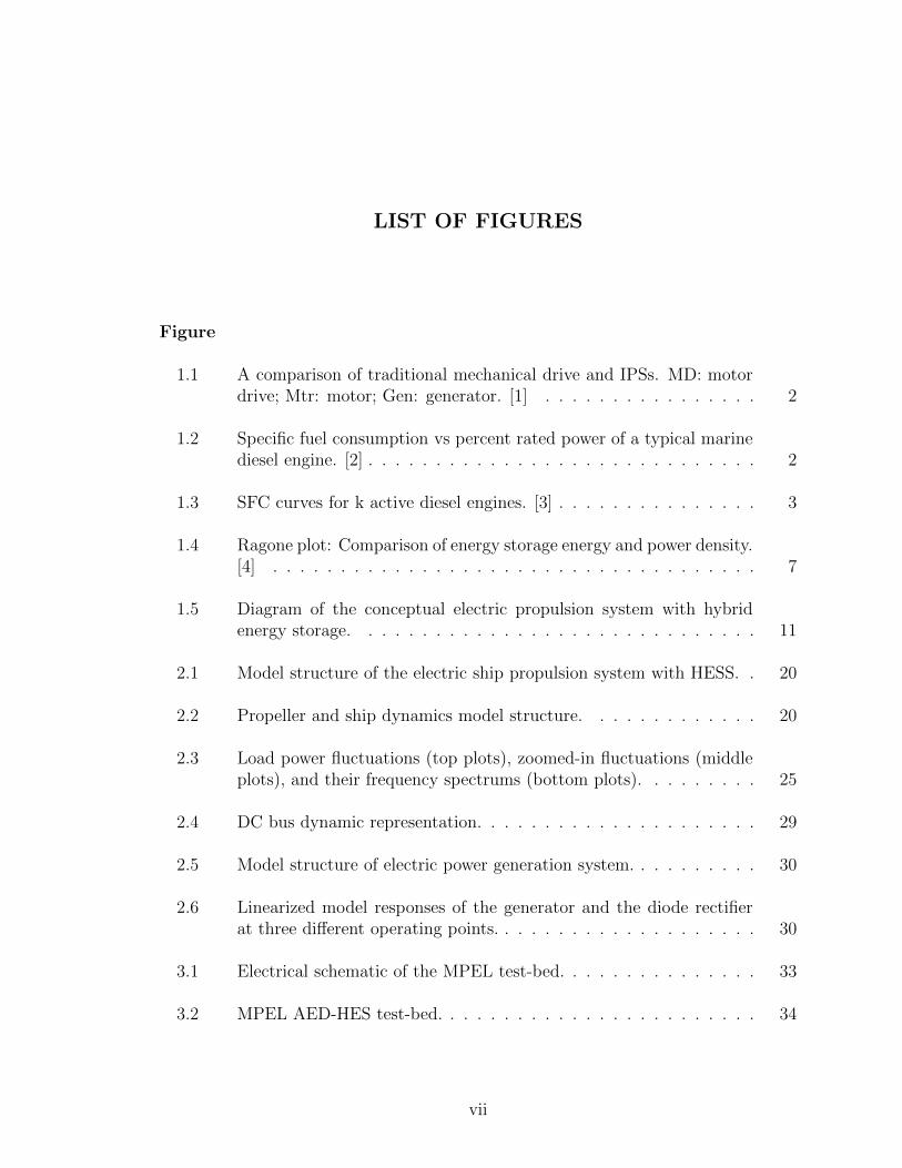
LIST OF FIGURES
Figure
1.1 A comparison of traditional mechanical drive and IPSs. MD: motordrive; Mtr: motor; Gen: generator. [1] . . . . . . . . . . . . . . . . 2
1.2 Specific fuel consumption vs percent rated power of a typical marinediesel engine. [2] . . . . . . . . . . . . . . . . . . . . . . . . . . . . . 2
1.3 SFC curves for k active diesel engines. [3] . . . . . . . . . . . . . . . 3
1.4 Ragone plot: Comparison of energy storage energy and power density.[4] . . . . . . . . . . . . . . . . . . . . . . . . . . . . . . . . . . . . 7
1.5 Diagram of the conceptual electric propulsion system with hybridenergy storage. . . . . . . . . . . . . . . . . . . . . . . . . . . . . . 11
2.1 Model structure of the electric ship propulsion system with HESS. . 20
2.2 Propeller and ship dynamics model structure. . . . . . . . . . . . . 20
2.3 Load power fluctuations (top plots), zoomed-in fluctuations (middleplots), and their frequency spectrums (bottom plots). . . . . . . . . 25
2.4 DC bus dynamic representation. . . . . . . . . . . . . . . . . . . . . 29
2.5 Model structure of electric power generation system. . . . . . . . . . 30
2.6 Linearized model responses of the generator and the diode rectifierat three different operating points. . . . . . . . . . . . . . . . . . . . 30
3.1 Electrical schematic of the MPEL test-bed. . . . . . . . . . . . . . . 33
3.2 MPEL AED-HES test-bed. . . . . . . . . . . . . . . . . . . . . . . . 34
vii

3.3 Flywheel module of MPEL test-bed. . . . . . . . . . . . . . . . . . . 38
3.4 Battery module of MPEL test-bed. . . . . . . . . . . . . . . . . . . 39
3.5 UC module of MPEL test-bed. . . . . . . . . . . . . . . . . . . . . . 40
3.6 Experimental setup for the energy cycling test using batteries andultra-capacitors. . . . . . . . . . . . . . . . . . . . . . . . . . . . . . 41
3.7 Multi-frequency load power fluctuations generated by the resistiveload bank. . . . . . . . . . . . . . . . . . . . . . . . . . . . . . . . . 41
3.8 DC bus voltage without HESS bus voltage regulators. . . . . . . . 41
3.9 Schematic of the independent bus voltage regulation control usingbatteries and ultra-capacitors. . . . . . . . . . . . . . . . . . . . . . 42
3.10 DC bus voltage with independent bus voltage regulators using bat-teries and ultra-capacitors: (a) bus voltage (left) and (b) UC voltage(right). . . . . . . . . . . . . . . . . . . . . . . . . . . . . . . . . . . 42
3.11 Schematic of the filter-based control using batteries and ultra-capacitors. 43
3.12 DC bus voltage with filter-based control using batteries and ultra-capacitors: (a) bus voltage (left) and (b) UC voltage (right). . . . . 43
3.13 Experimental setup for the energy cycling test using the flywheel andultra-capacitors. . . . . . . . . . . . . . . . . . . . . . . . . . . . . . 44
3.14 Schematic of the filter-based control using the flywheel and ultra-capacitors. . . . . . . . . . . . . . . . . . . . . . . . . . . . . . . . . 44
3.15 DC bus voltage with filter-based control using the flywheel and ultra-capacitors: (a) bus voltage (left) and (b) UC voltage (right). . . . . 45
4.1 Pareto-fronts of B/FW and B/UC HESS at sea state 2. . . . . . . . 50
4.2 Pareto-fronts of B/FW and B/UC HESS at sea state 4. . . . . . . . 51
4.3 Pareto-fronts of B/FW and B/UC HESS at sea state 6. . . . . . . . 51
4.4 Pareto-fronts of B/FW and B/UC HESS at sea states 2,4 and 6 withdifferent battery state of health. . . . . . . . . . . . . . . . . . . . . 56
viii

4.5 B/FW HESS performance at sea state 4 without any penalty on thespeed of FW. . . . . . . . . . . . . . . . . . . . . . . . . . . . . . . 58
4.6 The flywheel SOC of MOP dynamic programming solutions with dif-ferent initial SOCs. . . . . . . . . . . . . . . . . . . . . . . . . . . . 58
4.7 The performance comparison: MPC vs. DP. . . . . . . . . . . . . . 60
4.8 MPC (N=20, without UC SOC penalty) performance at sea state 4. 62
4.9 MPC (N=20, with UC SOC penalty) performance at sea state 4. . . 62
5.1 Control strategy diagram: left: PF-MPC, right: CC-MPC. . . . . . 65
5.2 Pareto-fronts of UC-Only, CC-MPC and PF-MPC at sea state 4(N=20). . . . . . . . . . . . . . . . . . . . . . . . . . . . . . . . . . 69
5.3 Pareto-fronts of UC-Only, CC-MPC and PF-MPC at sea state 6(N=20). . . . . . . . . . . . . . . . . . . . . . . . . . . . . . . . . . 70
5.4 CC-MPC and PF-MPC performance at sea state 4. . . . . . . . . . 71
5.5 Sensitivity analysis of predictive horizon for CC-MPC at sea state 4. 72
5.6 Sensitivity analysis of predictive horizon for CC-MPC at sea state 6. 73
5.7 Pareto-fronts of Case I and II at sea state 4 (N=20). . . . . . . . . . 74
5.8 Pareto-fronts of Case I and II at sea state 6 (N=20). . . . . . . . . . 74
5.9 The HESS output currents of CC-MPC (Case II) at sea state 4. . . 75
6.1 Schematic of the electric propulsion system with HESS control strate-gies for the comparative study. . . . . . . . . . . . . . . . . . . . . . 79
6.2 The block diagram of the feedback system with the baseline strategy. 80
6.3 The bus voltage response with the baseline strategy at sea state 4. . 81
6.4 Performance comparison of BL and MLF: bus voltage response (topplots) and their frequency spectrums (bottom plots) at sea state 4. . 82
6.5 The block diagram of the feedback system with the MLF strategy. . 83
6.6 Bode plot of load fluctuation response (LF → EDC) by BL and MLF. 83
ix

6.7 Performance comparison of BL and BVR: bus voltage response (topplots) and their frequency spectrums (bottom plots). . . . . . . . . 84
6.8 The block diagram of the feedback system for the BVR strategy. . . 85
6.9 Bode plot of load fluctuation response (LF → EDC) by BL and BVR. 85
6.10 Undesirable interaction: fluctuating currents from the generator andbattery pack for the system with BVR. . . . . . . . . . . . . . . . . 86
6.11 Performance comparison of BL and EMS: bus voltage response (topplots) and their frequency spectrums (bottom plots). . . . . . . . . 88
6.12 Performance comparison: BL, BVR and EMS. . . . . . . . . . . . . 90
6.13 Schematic of HESS-EMS for the electric propulsion system with HESS. 91
6.14 Schematic of SYS-EMS for the electric propulsion system with HESS. 93
6.15 Performance of HESS-EMS and SYS-EMS at Sea State 4. . . . . . . 97
6.16 Performance of HESS-EMS and SYS-EMS with pulse power load atSea State 4. . . . . . . . . . . . . . . . . . . . . . . . . . . . . . . . 98
7.1 Bode plot of the input observer. . . . . . . . . . . . . . . . . . . . . 107
7.2 Schematic diagram of the first approach (IO-LP). . . . . . . . . . . 107
7.3 Outputs of the detailed and simplified propeller-load torque modelsat sea state 4 (top) and sea state 6 (bottom). . . . . . . . . . . . . . 109
7.4 Schematic diagram of the AMPC controller. . . . . . . . . . . . . . 111
7.5 Estimation error of the adaptive load estimation and input observer. 113
7.6 Cases 2 and 3 degraded “Total Cost” performance compared to Case 1.115
7.7 Cases 4 and 5 degraded “Total Cost” performance compared to Case 1.115
7.8 Cases 2 and 4 degraded “Total Cost” performance compared to Case 1.116
7.9 Cases 3 and 5 degraded “Total Cost” performance compared to Case 1.117
x

7.10 Cases 2-6 degraded “Torque Oscillation Reduction” performance com-pared to Case 1. . . . . . . . . . . . . . . . . . . . . . . . . . . . . . 118
7.11 Torque comparison at sea states 4 and 6: Case 6 vs. Test 1. . . . . 120
8.1 Simplified DC bus dynamic model of the AED-HES test-bed. . . . . 124
8.2 Schematic of the filter-based control. . . . . . . . . . . . . . . . . . 125
8.3 Schematic of the real-time MPC. . . . . . . . . . . . . . . . . . . . 126
8.4 Flowchart of the IPA-SQP algorithm [5]. . . . . . . . . . . . . . . . 128
8.5 Hierarchical control structure for real-time control implementation. . 129
8.6 Circuit diagram of bi-directional DC/DC converters for HESS. . . . 129
8.7 The implementation of Speedgoat controller. . . . . . . . . . . . . . 131
8.8 Matlab/Simulink program of the local controllers. . . . . . . . . . . 132
8.9 Control performance: battery and UC command power and actualpower (zoom-in plots in the bottom). . . . . . . . . . . . . . . . . . 133
8.10 Multi-core structure of Speedgoat. . . . . . . . . . . . . . . . . . . . 134
8.11 Real-time simulation evaluation of system-level controller (core1). . 134
8.12 Real-time simulation evaluation of component-level controllers (core2).134
8.13 Diagram of real-time MPC experiment. . . . . . . . . . . . . . . . . 136
8.14 Experimental results of sea state 4: MPC vs. filter-based control . . 136
8.15 Experimental results of sea state 6: MPC vs. filter-based control. . 137
8.16 Experimental results of pulse power load: MPC vs. filter-based control.138
8.17 Experimental results of sea state 4: MPC(N=20) vs. MPC(N=40). . 139
8.18 Experimental results of sea state 6: MPC(N=20) vs. MPC(N=40). . 140
8.19 Experimental results of pulse power load: MPC(N=20) vs. MPC(N=40)141
xi

8.20 UC output current and the number of iteration to solve the optimiza-tion problem. . . . . . . . . . . . . . . . . . . . . . . . . . . . . . . 141
8.21 Real-time simulation comparison of maximum execution time. . . . 142
xii

LIST OF TABLES
Table
1.1 The characteristics of battery, UC and flywheel. . . . . . . . . . . . 8
2.1 Ship parameters . . . . . . . . . . . . . . . . . . . . . . . . . . . . . 24
2.2 Hybrid energy storage parameters. . . . . . . . . . . . . . . . . . . . 27
2.3 Requirement based on sea state 4 . . . . . . . . . . . . . . . . . . . 28
2.4 HESS configuration and size selection. . . . . . . . . . . . . . . . . . 28
3.1 Manufacturer specifications for system controller. . . . . . . . . . . 35
3.2 Manufacturer specifications for electric machines. . . . . . . . . . . 36
3.3 Manufacturer specifications for flywheel. . . . . . . . . . . . . . . . 37
3.4 Specifications for the battery system. . . . . . . . . . . . . . . . . . 39
3.5 Specifications for the ultra-capacitors. . . . . . . . . . . . . . . . . . 39
4.1 Performance metrics. . . . . . . . . . . . . . . . . . . . . . . . . . . 52
4.2 Performance comparison of the selected design points. . . . . . . . . 53
4.3 Performance comparison of the proposed MPC and DP. . . . . . . . 61
6.1 Properties of control strategies. . . . . . . . . . . . . . . . . . . . . 79
6.2 Performance comparison of different control strategies. . . . . . . . 89
6.3 EMS performance comparison. . . . . . . . . . . . . . . . . . . . . . 100
xiii

7.1 Control objectives and their mathematical expression. . . . . . . . . 102
7.2 Performance metrics. . . . . . . . . . . . . . . . . . . . . . . . . . . 111
7.3 Performance comparison. . . . . . . . . . . . . . . . . . . . . . . . . 114
7.4 Performance comparison: Case 6 vs. Case 1 with 2% modeling error. 119
7.5 Performance comparison: weighting factor effects. . . . . . . . . . . 119
8.1 Performance comparison: filter-based vs. MPC. . . . . . . . . . . . 135
8.2 Performance comparison: MPC(N=20) vs. MPC(N=40). . . . . . . 139
xiv

LIST OF ABBREVIATIONS
AED Advanced Electric Drive
AES All-Electric Ship
AMPC Adaptive Load Estimation/Prediction with Model Predictive Control
BCM Battery Control Module
BMS Battery Management System
BVR Bus Voltage Regulation
B/FW Battery with Flywheel
B/UC Battery with Ultra-capacitor
CC Coordinated Control
CPP Controllable Pitch Propeller
EMS Energy Management Strategy
ESD Energy Storage Device
FPP Fixed Pitch Propeller
HESS Hybrid Energy Storage System
HEV Hybrid electric vehicle
IM Induction Machine
IO Input Observer
IPS Integrated Power System
LP Linear Prediction
LPC Linear Prediction Coefficient
xv

MLF Motor Load Following
MOP Multi-objective Optimization Problem
MPC Model Predictive Control
MPEL University of Michigan Power and Energy Lab
PM Prime Mover
PF Pre-filtering
RMS Root Mean Square
UPS Uninterruptible Power Supply
SOC State of Charge
SQP Sequential Quadratic Programming
SS Sea State
UC Ultra-capacitor
VSD Variable Speed Drives
xvi

ABSTRACT
Electric ships experience large propulsion-load fluctuations on their drive shaft
due to encountered waves and the rotational motion of the propeller, affecting the re-
liability of the shipboard power network and causing wear and tear. This dissertation
explores new solutions to address these fluctuations by integrating a hybrid energy
storage system (HESS) and developing energy management strategies (EMS). Ad-
vanced electric propulsion drive concepts are developed to improve energy efficiency,
performance and system reliability by integrating HESS, developing advanced control
solutions and system integration strategies, and creating tools (including models and
testbed) for design and optimization of hybrid electric drive systems.
A ship dynamics model which captures the underlying physical behavior of the
electric ship propulsion system, is developed to support control development and
system optimization. To evaluate the effectiveness of the proposed control approaches,
a state-of-the-art testbed has been constructed which includes a system controller, Li-
Ion battery and ultra-capacitor (UC) modules, a high-speed flywheel, electric motors
with their power electronic drives, DC/DC converters, and rectifiers.
The feasibility and effectiveness of HESS are investigated and analyzed. Two
different HESS configurations, namely battery/UC (B/UC) and battery/flywheel
(B/FW), are studied and analyzed to provide insights into the advantages and limi-
tations of each configuration. Battery usage, loss analysis, and sensitivity to battery
aging are also analyzed for each configuration. In order to enable real-time applica-
tion and achieve desired performance, a model predictive control (MPC) approach
is developed, where a state of charge (SOC) reference of flywheel for B/FW or UC
xvii

for B/UC is used to address the limitations imposed by short predictive horizons,
because the benefits of flywheel and UC working around high efficiency range are ig-
nored by short predictive horizons. Given the multi-frequency characteristics of load
fluctuations, a filter-based control strategy is developed to illustrate the importance
of the coordination within the HESS. Without proper control strategies, the HESS
solution could be worse than a single energy storage system solution.
The proposed HESS, when introduced into an existing shipboard electrical propul-
sion system, will interact with the power generation systems. A model-based analysis
is performed to evaluate the interactions of the multiple power sources when a hybrid
energy storage system is introduced. The study has revealed undesirable interactions
when the controls are not coordinated properly, and leads to the conclusion that a
proper EMS is needed.
Knowledge of the propulsion-load torque is essential for the proposed system-level
EMS, but this load torque is immeasurable in most marine applications. To address
this issue, a model-based approach is developed so that load torque estimation and
prediction can be incorporated into the MPC. In order to evaluate the effectiveness
of the proposed approach, an input observer with linear prediction is developed as
an alternative approach to obtain the load estimation and prediction. Comparative
studies are performed to illustrate the importance of load torque estimation and
prediction, and demonstrate the effectiveness of the proposed approach in terms of
improved efficiency, enhanced reliability, and reduced wear and tear.
Finally, the real-time MPC algorithm has been implemented on a physical testbed.
Three different efforts have been made to enable real-time implementation: a specially
tailored problem formulation, an efficient optimization algorithm and a multi-core
hardware implementation. Compared to the filter-based strategy, the proposed real-
time MPC achieves superior performance, in terms of the enhanced system reliability,
improved HESS efficiency, and extended battery life.
xviii

CHAPTER I
Introduction
1.1 Background
1.1.1 All-Electric Ships with Integrated Power System
Electric propulsion in marine applications is not a new concept, dating back over
100 years [6, 7, 8]. Recently, marine electrification has become increasingly popular
after the development of high power variable speed drives (VSDs) in the 1970’s-1980’s
[6, 9, 10]. With the introduction of VSDs, a common set of generators could power
both the ship service and propulsion systems. This concept is referred to as an
integrated power system (IPS), which is the characterizing element of an all-electric
ship (AES) [1, 9, 10, 11, 12]. The comparison of traditional mechanical drive and
IPSs is shown in Figure 1.1.
The IPS architecture provides the electrical power for both ship service and electric
propulsion loads by integrating power generation, distribution, storage and conver-
sion. Compared to the traditional mechanical drive, the benefits of IPS are summa-
rized in the following:
• IPS improves the efficiency of the prime movers [1, 2, 3, 6, 7, 13, 14, 15]: The
optimal operating power of marine diesel engines is typically between 70%-90%
of their rated power; however, they often operate at 20-50% of their rated power
1

Figure 1.1: A comparison of traditional mechanical drive and IPSs. MD: motor drive;Mtr: motor; Gen: generator. [1]
Figure 1.2: Specific fuel consumption vs percent rated power of a typical marine dieselengine. [2]
[2], especially for large military ships. The specific fuel consumption of a typical
marine diesel engine is shown in Figure 1.2. Since the prime movers do not
2

Figure 1.3: SFC curves for k active diesel engines. [3]
operate in their most efficient speed and power range under many operating
conditions, the overall prime mover efficiency can be significantly degraded.
IPS is able to optimize the number of operating prime mover and generator sets
based on the overall power of the propulsion system and ship service systems.
For example, as shown in Figure 1.3 [3], when the total power requirement is
less than 300kW, only 1 prime mover and generator set will operate; if it is
between 300kW and 500kW, then 2 generators are preferred. Therefore, the
overall system efficiency of an IPS configuration can be considerably higher
than that of an equivalent mechanical drive design, particularly at low power
levels. As a result, fuel consumption and emissions are reduced [6].
• IPS improves the efficiency of the propulsors [1, 13, 15]: In an integrated power
system, the traditional controllable-pitch propeller (CPP) in the propulsion-
shaft line can be replaced by a high-efficiency fixed-pitch propeller (FPP). The
CPP is able to control the ship’s speed, both forward and reverse. This is im-
portant when the propeller is coupled with prime movers such as diesel engines
and gas turbines that are not reversible and may have a minimum operating
3

rotational speed. Compared to FPP, CPP needs a large hub to hold the appa-
ratus in order to adjust its pitch. Due to this large hub, the efficiency of CPP
will be reduced. In contrast, the motors in IPS are able to operate from zero
to their maximum speed for both forward and reverse operation. As a result of
this characteristic, a high-efficiency FPP can be employed in IPS.
• IPS provides flexibility of arrangements [1, 7, 13, 14, 16]: For the electrical
network, the prime mover and generator sets can be placed almost anywhere,
which offers flexibility to the designers. Furthermore, long shaft lines can be
simplified with direct motor drives, leading to space saving.
• IPS improves the survivability of electrical systems [1, 7, 14, 15, 16, 17]: IPS
supports zonal survivability, which is the ability of a distributed system to
ensure that loads in one zone do not experience a service interruption by faults
which occurs in other zones. Zonal survivability also facilitates the ship’s ability
to maintain or restore the damaged zones without interrupting other zones.
• IPS supports high-power mission systems, such as high-power radar and weapon
systems [1, 15]: As the demand of power missions increases [4, 18], it is essential
to support high-power mission systems for future naval ships. IPS outperforms
traditional mechanical drives in coordinating the propulsion system with ship
service systems. Usually, the need for high-power mission systems is not re-
quired at the same time as maximum propulsion. The power sharing ability
of IPS requires less generator sets than non-integrated power systems to sup-
port the same high-power mission systems, contributing to acquisition savings,
reduced maintenance costs, and reduced volume.
• IPS offers a more comfortable residential environment [15, 16]: Because of the
reduction of mechanical equipment, such as long shafts and large gearboxes,
noise and vibration, can be significantly attenuated by an electric propulsion
4

system. This is one of the main reasons that IPS has become standard in large
cruise ships [16].
IPS provides considerable benefits to modern ships; at the same time, it faces
challenges. One of these challenges is propulsion load fluctuations from the propeller.
These load fluctuations do not affect the electrical shipboard network in traditional
mechanical drives, because the fluctuations are isolated by the non-integrated power
system. For the integrated power system, however, these fluctuations can affect the
electrical shipboard network.
Three different types of propulsion load fluctuation are studied in the literature
[19, 20, 21, 22, 23, 24, 25, 26]:
• fluctuations from the impact of the first order wave at the encounter wave
frequency (load periods typically from seconds to minutes),
• fluctuations from the in-and-out-of-water effect (load periods in seconds),
• fluctuations caused by the propeller rotation at the propeller-blade frequency
(i.e. number of blades times shaft speed in revolutions per second).
The impact of the encounter-wave-frequency fluctuations combined with the in-
and-out-of-water effect has also been reported in the literature [19, 20, 21, 22, 23].
These fluctuations, especially when the propeller is in-and-out-of-water, will signifi-
cantly reduce electrical efficiency, affect power quality on the shipboard power net-
work, and cause wear and tear. The fluctuations caused by the in-and-out-of-water
effect can be as high as 100% of the nominal power. These two load fluctuations are
defined as low-frequency fluctuations in this dissertation.
The high-frequency fluctuation discussed in this dissertation is at the propeller-
blade frequency (i.e. number of blades times shaft speed in rps) [19, 20, 21, 22].
This fluctuation, caused by the wake field, has been discussed in [24]. The Fourier
5

analysis of the wake field, discussed in Chapter 5 of [25], is used to capture these high-
frequency dynamics. It it worth noting that the fluctuations at the propeller-blade
frequency can be very significant during ventilation [19]. The experimental results of
the propeller at both non-ventilation and ventilation conditions were provided by [26],
where significantly large torque fluctuations at both high and low frequencies were
observed. The importance of the mechanical effects caused by the propeller-blade
frequency fluctuations has been discussed in [19, 20, 21, 22]. This high-frequency
fluctuation is reported as one of the main causes for severe mechanical wear and tear
of the propulsion unit. The impact on the electrical system, however, highly depends
on the propeller inertia and the associated controller.
1.1.2 Energy Storage Devices for All-Electric Ships
The importance of Energy Storage Device (ESD) development in the electrifica-
tion of ships is highlighted in the Naval Next Generation Integrated Power System
Technology Development Roadmap in 2007 and 2013 [4, 18], where batteries, ultra-
capacitors (UCs), and flywheels are discussed as possible ESDs. The battery is an
electrochemical device with high energy density but relatively poor power density. In
contrast, ultra-capacitors store energy in an electric field without chemical reactions,
while flywheels store energy mechanically in the form of kinetic energy, both yielding
power densities that are much higher than that of batteries. However, their lower
energy densities make ultra-capacitors and flywheels unsuitable for sustained oper-
ation. The Ragone plot of batteries, ultra-capacitor (double-layer capacitors) and
flywheel is shown in Figure 1.4. These complementary characteristics of batteries,
ultra-capacitors, and flywheels suggest that different combinations of ESDs should
be considered for different applications [4, 27]. Only using one single type of ESD
can result in increased size, weight and cost for electric ship operations [28]. The
combination of different ESDs is defined as a Hybrid Energy Storage System (HESS).
6

Figure 1.4: Ragone plot: Comparison of energy storage energy and power density. [4]
ESDs (namely batteries, UCs and flywheels) and their combinations (i.e., HESS)
have been explored by the automotive, power system and control engineering commu-
nities. ESDs and HESSs are widely used in applications, such as electric/hybrid elec-
tric vehicles [29, 30, 31, 32, 33, 34, 35], micro grids [36, 37, 38, 39], and uninterruptible
power supplies (UPS) [4, 40]. However, the ESDs/HESSs in marine applications are
still understudied [4]. The potential benefits of integrating ESDs/HESSs have been
reported in the literature. In order to support pulse power loads, such as high-power
radar and lasers, UCs have been used in [41, 42] and flywheels have been studied in
[43, 44, 45]. The combination of the battery, UC and flywheel for mitigating pulse
power loads is studied in [46]. Note that the studies in [41, 43, 44, 45, 46] are based
on simulations, while the approach in [42] is experimentally validated. In order to
reduce wear and tear on the generator sets, batteries are used in [2, 47] to “smooth”
the generator power. In [17], battery modules are used to assist the turbine and
fuel cell in tracking the power command. The reduction of fuel consumption using
ESD/HESS has been explored in [3, 48, 49, 50]. A battery ESD is used in [3], and an
HESS, which combines batteries with UCs, is studied in [48, 49, 50]. In order to ad-
dress propulsion load fluctuations, batteries, UCs, flywheels and their combinations,
7

i.e., HESS, have been studied in [51, 52, 53, 54, 55].
According to the literature review, UCs and flywheels are the best candidate for
mitigating pulse power effects. This is because the pulse power load is usually of
high power and short duration. The UC and flywheel have higher power density
than the battery. Additionally, the UC and flywheel have fast dynamic response to
compensate the pulse power load. For a long-duration load, the battery is preferred
due to its high energy density. Compared to UC and flywheel, however, the main
disadvantages of the battery are its relatively short cycle life and limited recharge
rate. Furthermore, as the capacity of the battery degrades, the internal resistance
will be increased, leading to increased losses. In order to address the limitations of
the battery, the HESS, thanks to its complementary characteristic, is one of the most
popular solutions. The characteristics of each ESD are summarized in Table 1.1.
Note that the preferred characteristics are in blue and undesirable ones are in red.
Table 1.1: The characteristics of battery, UC and flywheel.Battery UC Flywheel
Energy density High Low MediumPower density Low High MediumCycle life Short Medium LongRecharge rate Low High MediumSelf-discharge Low Medium High
1.1.3 Energy Management for All-Electric Ships
Energy/power management strategies coordinate multiple power sources and mul-
tiple power loads, in order to achieve robust and efficient operation and to meet var-
ious dynamic requirements. An effective energy management system is needed to
provide improved fuel efficiency, enhanced response speed, superior reliability and
reduced mechanical wear and tear [17, 42, 47, 56]. In order to achieve these expec-
tations, optimization-based energy management is required to address the trade-offs
among these objectives. Furthermore, optimization-based energy management is also
8

suggested in the Naval Power Systems Technology Development Roadmap [4]. The
characteristics of IPS in all-electric ships have been summarized in [56], including:
• Nonlinear and multi-input-and-multi-output plant characteristics;
• Reconfigurable underlying physical components;
• Multi-scale time dynamics;
• Multiple operating constraints.
These characteristics suggest model predictive control (MPC) as a natural choice
for optimization-based energy management strategies. Energy management strate-
gies using MPC have been investigated in the literature. A sensitivity-function-based
approach is proposed in [17], which achieves real-time trajectory tracking. In [42, 57],
a nonlinear MPC is developed to compensate pulse power loads and follow the desired
references, including the desired bus voltage, desired reference power for generator sets
and desired reference speed for the motor. In [47], a stochastic MPC is developed to
smooth out power fluctuations. A multi-level MPC is used in [50] to address distur-
bances from the environment. The main challenge to implement the model predictive
control approaches discussed above is to solve the optimization problem in real-time
within a relatively short sampling time. In order to evaluate the effectiveness of the
proposed approach, the energy management strategy developed in this dissertation
is implemented on a test-bed. To our best knowledge, the study in [42] is the only
one prior to this work, which has demonstrated the feasibility of optimization-based
shipboard energy management with test results on a physical platform.
1.2 Motivation
Ship electrification has been a technological trend in commercial and military ship
development in response to recent energy efficiency and environmental protection ini-
9

tiatives [4, 18]. Electric propulsion plays a central role in this design paradigm shift.
The introduction of electric propulsion has brought about new opportunities for tak-
ing a fresh look at old problems and developing new solutions. Thrust and torque
fluctuations due to the hydrodynamic interactions and wave excitations have been
identified as inherent elements in the ship propulsion system [19, 20, 24, 26, 58]. As
discussed in Section 1.1.1, three different propulsion load fluctuations are studied in
this research: fluctuations from the impact of the first order wave at the encounter
wave frequency, fluctuations from the in-and-out-of-water effect (load periods in sec-
onds) and fluctuations at the propeller-blade frequency (i.e. number of blades times
shaft speed in rps). These fluctuations significantly affect the performance and life
cycle of both mechanical and electrical systems involved, as has been analyzed in
[21, 22, 23, 59]. For mechanical systems, excessive fluctuations on torque and power
will increase mechanical stress and cause wear and tear. The importance of the me-
chanical effects caused by propeller-blade frequency fluctuations has been discussed
in [19, 20, 21, 22]. For electrical systems, power fluctuations, especially when the pro-
peller is in-and-out-of-water, will reduce electrical efficiency and affect power quality
on the shipboard power network [19, 20, 21, 22, 23, 24, 25, 26]. In order to address
these issues, several studies have been discussed in the literature, such as using thrust
control for power smoothing [19, 20]. The trade-offs between speed control, torque
control, and power control of the motor have been studied in [19]. Using thruster bi-
asing for vessels with dynamic positioning systems has been proposed in [60, 61, 62] to
reduce load fluctuations. These methods deal primarily with low-frequency variations
and are typically applied to dynamic positioning systems.
In order to address the load fluctuations, a hybrid energy storage system solu-
tion is proposed. The concept of the proposed system is shown in Figure 1.5. The
energy storage elements serve as a buffer to absorb energy when the motor is under-
loaded and supply energy when overloaded, thereby isolating the power network from
10

DC BusElectric
Machine
Variable
Speed
Drive
Ultracap
Energy
Storage
System
Flywheel
Energy
Storage
System
External
Power
Controller
Control Signals
Battery
Energy
Storage
System
Power Flow
Figure 1.5: Diagram of the conceptual electric propulsion system with hybrid energystorage.
propulsion load fluctuations and improving overall system efficiency. Using different
energy storage mechanisms allow one to exploit their different characteristics to ad-
dress different frequency components in the power and thrust fluctuations. Besides
the well-configured HESS, the integration and operation of a shipboard electrical
propulsion system with HESS relies on effective power/energy management strate-
gies in order to mitigate the load power fluctuation effects and achieve the desired
benefits, in terms of increased system efficiency, improved reliability, and reduced
wear and tear. To improve the robustness of the control strategy, addressing the un-
certainties in the model, especially in the propulsion load torque model, is one of the
key issues. Furthermore, a physical test-bed is required for implementing the control
strategies in real-time and evaluating their effectiveness. In summary, the motivation
of this research is to answer the following questions:
• How to capture the underlying dynamics in the electric ship propulsion sys-
tem, especially the propulsion load dynamics, to support control and system
integration?
• How to evaluate the benefits and limitations of different energy storage/hybrid
11

energy storage configurations?
• How to develop an energy management strategy to achieve the desired perfor-
mance?
• How to accurately estimate and predict the propulsion load torque and demon-
strate robustness of the energy management solution?
• How to build a physical test-bed for implementing and evaluating the proposed
approaches?
1.3 Main Contributions
This research aims to address propulsion load fluctuations in all-electric ships with
HESS. Although HESS has been investigated in many applications, such as hybrid
electric vehicle, this is the first attempt to exploit HESS to address propulsion-load
fluctuations in all-electric ships. Configuration optimization and energy management
strategy development has been studied. A coordinated approach is used to exploit the
complementary characteristics of HESS. A system-level energy management strategy
is developed using model predictive control. This strategy encompasses the controls of
the primary power sources and propulsion motor, in addition to the HESS, and allows
judicious coordination to achieve desired performance in terms of increased system
efficiency, enhanced reliability, reduced mechanical wear and tear, and improved load-
following capability. The main contributions of this research are summarized in the
following:
1) Model development [63]: To support research activities associated with the
control and optimization of electric ship propulsion systems, a control- and
optimization-oriented model is an essential tool for feasibility analysis and sys-
tem design. The models developed in this dissertation include the propeller
12

and ship dynamic model, hybrid energy storage models, the diesel engine and
generator set model, electrical motor models and the DC bus dynamic model.
The main contribution of model development is the propeller and ship dynamic
model. To the best knowledge of the author, this is the first model to capture
both high- and low-frequency load fluctuations on the propeller.
2) Test-bed development [64, 65]: In order to provide a flexible hardware envi-
ronment for testing and validation of control algorithms for electric propulsion
systems with HESS, the Advanced Electric Drive with Hybrid Energy Storage
test-bed has been constructed in the University of Michigan Power and Energy
Lab (MPEL). This state-of-the-art test-bed, which includes a system controller,
Li-Ion battery modules, ultra-capacitor modules, a high speed flywheel, perma-
nent magnet motors, induction motors, DC/DC converters, and three-phase
inverters, is uniquely designed for HESS development to address the load fluc-
tuation problem in electric ship propulsion systems. The test-bed will be used
to implement and validate the proposed control approaches.
3) Evaluation of energy storage configurations [53, 66]: Since there is no literature
to report the effectiveness of HESS in addressing the multi-frequency propulsion-
load fluctuation problem for all-electric ships, we first explore the HESS solution
as a buffer to isolate the load fluctuations from the shipboard power network.
Two different HESS configurations, namely battery combined with UC and
battery combined with flywheel, are studied. We first quantitatively analyze the
performance of these two configurations and provide insights into the advantages
and limitations of each configuration. The battery usage, loss analysis, and
sensitivity to battery aging of these two configurations are also analyzed.
4) Control development and performance evaluation of HESS [51, 52, 66, 67]: In or-
der to enable real-time applications and achieve desired performance, a model
13

predictive control (MPC) strategy is developed. In this MPC formulation, a
state of charge (SOC) reference is used to address the limitations imposed by
short predictive horizons. Furthermore, because of the multi-frequency char-
acteristics of load fluctuations, a filter-based control strategy is investigated to
illustrate the importance of coordination. Without proper control strategies, the
HESS solution could be worse than a single ESD solution. The proposed MPC
and filter-based control strategies are implemented on the physical testbed. The
experimental results demonstrate the effectiveness of the proposed MPC strat-
egy.
5) Development of energy management strategy [54, 55]: When the HESS is in-
troduced into the existing system, there are two potential configurations: a
‘plug-in configuration’ and an ‘integrated configuration’. For ‘plug-in’ configu-
ration, a novel energy management strategy is developed to avoid undesirable
interactions between multiple energy sources. Compared to conventional strate-
gies, the comparison study demonstrates the effectiveness of the proposed en-
ergy management strategy. For ‘integrated configuration’, an integrated energy
management strategy is developed to fully coordinate generator sets, HESS, and
motor drive. A cost function is formulated to achieve desirable performance in
terms of improved efficiency, enhanced reliability, and reduced mechanical wear
and tear.
6) Estimation and prediction of propulsion-load torque [68]: The propulsion-load
torque is not measurable in most marine applications. To address this issue,
we develop a model-based approach to estimate the propulsion-load torque for
all-electric ships. Due to the complexity of the propulsion-load torque model,
we first develop a simplified model which is able to capture the key dynamics,
including both high- and low-frequency load fluctuations. Because of uncer-
14

tainties in the model parameters, adaptive load estimation is used, leading to
improved control performance. This model-based approach can be easily inte-
grated with the MPC to formulate an adaptive load estimation/prediction with
MPC (AMPC).
Most of the results outlined above have been documented and published in archived
journals and/or referred conference proceedings [51, 52, 53, 54, 55, 63, 64, 69]. Other
results are under reviewed or preparation for archived journals [65, 66, 67, 68].
1.4 Outline
The dissertation is organized as follows:
In Chapter II, control-oriented models are presented for all-electric ships with
hybrid energy storage. These models include the propeller and ship dynamic model,
hybrid energy storage models, the diesel engine and generator set model, electrical
motor models and the DC bus dynamic model.
Chapter III presents the development of the Advanced Electric Drive with Hy-
brid Energy Storage test-bed for electric ship propulsion systems at the University of
Michigan Power and Energy Lab. To address load fluctuations in electrical propul-
sion systems, this test-bed is developed to validate modeling and control solutions.
Experimental test results, which demonstrate the energy cycling capability of the
test-bed to mitigate the impact of load fluctuations on the bus, are documented in
this chapter.
Chapter IV evaluates different HESS configurations and provides the insights into
the advantages and limitations of each HESS configuration. Two main objectives are
power-fluctuation compensation and HESS loss minimization. Since these objectives
conflict with each other in the sense that effective compensation of fluctuations will
lead to HESS losses, the weighted-sum method is used to convert this multi-objective
15

optimization problem (MOP) into a single-objective problem. Global optimal solu-
tions are obtained using dynamic programming (DP) by exploiting the periodicity of
the load. These global optimal solutions form the basis of a comparative study of
B/FW and B/UC HESS, where the Pareto fronts of these two technologies at different
sea state (SS) conditions are derived. The analysis aims to provide insights into the
advantages and limitations of the B/FW and B/UC HESS solutions. To enable real-
time application and achieve desired performance, a model predictive control (MPC)
strategy is developed. In this MPC formulation, a state of charge (SOC) reference is
used to address the limitations imposed by short predictive horizons.
Chapter V evaluates the control strategies of HESS. Since the effectiveness of
HESS highly depends on its control strategies, two strategies for real-time energy
management of HESS are analyzed in this chapter. The first one splits the power
demand such that high- and low-frequency power fluctuations are compensated by
fast- and slow-dynamic energy storage devices, respectively; the second considers the
HESS as a single entity and coordinates the operations of the hybrid energy storage
system. Results show that the coordination within HESS provides substantial bene-
fits in terms of reducing power fluctuation and losses. The battery/ultra-capacitors
(B/UC) configuration is used to elucidate the control implications in this chapter.
Chapter VI introduces two approaches to integrate the new HESS with an existing
propulsion system: the first one is defined as a ‘plug-in approach’, i.e., the new HESS
controller does not change the existing propulsion system; the other one is defined
as an ‘integrated approach’, in which a new integrated controller is developed for the
HESS and propulsion system. For the plug-in approach, the interaction analysis of
different control strategies is performed. The integrated approach takes advantage
of the predictive nature of MPC and allows the designers to judiciously coordinate
the different entities of the shipboard network under constraints, thereby providing
benefits to system performance.
16

In Chapter VII, load torque estimation and prediction for implementing MPC-
based energy management strategies is addressed. An AMPC approach is developed
to estimate the unknown parameters in the propulsion-load model. Due to the com-
plexity of the propulsion-load torque model, a simplified model is developed for the
proposed AMPC to capture the key dynamics. In order to evaluate the proposed
AMPC approach, an alternative approach is developed where an input observer (IO)
is used to estimate the propeller-load torque, and a linear prediction is combined
with the IO to predict the future load torque. A comparative study is performed
to evaluate the effectiveness of the proposed AMPC, in terms of minimizing the bus
voltage variation, regulating the rotational speed, and reducing the high-frequency
motor torque variations. The implications of accurate estimation and prediction are
also illustrated and analyzed in this study.
In Chapter VIII, real-time MPC is implemented on an AED-HES testbed. In
order to achieve real-time feasibility, three different efforts have been made: properly
formulating the optimization problem, identifying efficient optimization algorithm,
and exploiting a multi-core system controller. First, a problem formulation of the
proposed CC-MPC is crafted to achieve the desired performance with a relatively
short predictive horizon. Then, an integrated perturbation analysis and sequential
quadratic programming (IPA-SQP) algorithm is developed to solve the optimization
problem with high computational efficiency. Finally, a multi-core code structure is
developed for the real-time system controller to guarantee system signal synchroniza-
tion and to separate system-level and component-level controls, thereby increasing
the real-time capability. Compared with the filter-based control strategy, the im-
provements provided by the proposed real-time MPC demonstrated on the testbed
can be over 50% in terms of reduced bus voltage variations, reduced battery peak
and RMS currents, and reduced HESS losses. Furthermore, given the uncertainties
presented in any testbed, the experimental results also demonstrate the robustness of
17

the real-time MPC.
Chapter IX provides conclusions and presents future research directions.
18

CHAPTER II
Dynamic Model of An Electric Ship Propulsion
System with Hybrid Energy Storage
The schematic of the electric propulsion system under investigation is shown in
Figure 2.1. The system consists of a prime mover and a generator (PM/G) for power
generation, an electric motor for propulsion, the ship and its propeller, and a hybrid
energy storage system (HESS). Note that the battery/ultra-capacitor HESS is used as
an example in Figure 2.1. Power converters (i.e., DC/DC and AC/DC converters) are
used to connect electrical components. The modeling of each component is described
in this chapter and the resulting control-oriented models are presented.
2.1 Propeller and Ship Dynamic Model
The focus of the propeller and ship dynamic model is to capture the dynamic
behavior of the propeller and ship motion, including the power and torque fluctuations
induced on the motor drive shaft. The characteristics of the propeller, subject to the
wake field and in-and-out-of-water effects, are investigated and simulation results
are presented. As shown in Figure 2.2, the ship dynamics, propeller characteristics,
and motor dynamics are mechanically coupled; they influence each other through
mechanical connections and internal feedback [63].
19

Figure 2.1: Model structure of the electric ship propulsion system with HESS.
Figure 2.2: Propeller and ship dynamics model structure.
2.1.1 Propeller Characteristics
The propeller responses, in terms of thrust T and torque Q, are nonlinear functions
of propeller rotational speed n (in rps), ship speed U , and propeller parameters (e.g.
pitch ratio, propeller diameter, loss factor). In this work, we assume that the propeller
speed n is kept at the nominal set point and address the load power fluctuation
problem by integrating an HESS system and developing an optimized control solution
to manage the power.
The thrust, torque, and power can be expressed as:
T = sgn(n)βρn2D4fKT(JA, P itch/D,Ae/Ao, Z,Rn) , (2.1)
20

Q = sgn(n)βρn2D5fKQ(JA, P itch/D,Ae/Ao, Z,Rn) , (2.2)
P = 2π sgn(n)βρn3D5fKQ(JA, P itch/D,Ae/Ao, Z,Rn) , (2.3)
where β is the loss factor, ρ is the density of water, D is the diameter of the propeller,
and fKTand fKQ
are the functions of thrust and torque coefficients, respectively [70]-
[71].
In fKTand fKQ
, JA is the advance coefficient, Pitch/D is the pitch ratio, Ae/A0 is
the expanded blade-area ratio, with Ae being the expanded blade area and A0 being
the swept area, Z is the number of propeller blades, and Rn is the Reynolds number.
The parameters of the propeller used in this dissertation are listed in Table 2.1.
The loss factor β is used to account for the torque and thrust reduction experienced
by the propeller when it goes in-and-out-of-water.
In our case, we assume βT = βQ = β, and the dynamic effects of ventilation and
lift hysteresis are neglected. The effects of propeller in-and-out-of-water motion and
the sensitivity to submergence, however, will be captured in the loss factor using the
following expression, originally given in [21]:
β =
0, h/D ≤ −0.24;
1− 0.675(1− 1.538h/D)1.258, −0.24 < h/D < 0.65;
1, h/D ≥ 0.65;
(2.4)
where h is the propeller shaft submergence. A positive value of h means that the
propeller stays in the water, and a negative value means the propeller is out of the
water.
To complete the propeller model, one needs to know Va, the advance speed, in
order to calculate the advance coefficient JA = Va
nD. Note that the wake field, defined
21

as w = U−Va
U, should be taken into account. The wake field model is taken from [25],
which includes the average and fluctuation components. In this model, we assume that
the fluctuation component consists of 5 terms which are harmonic to the fundamental
cos(θ), given as follows:
w =1
Z
Z−1∑i=0
[0.2 + 0.12cos(θ − i
2π)
+ 0.15cos(2θ − 2i
2π) + 0.028cos(3θ − 3i
2π)
+ 0.035cos(4θ − 4i
2π)− 0.025cos(5θ − 5i
2π)],
(2.5)
where θ ∈ [0, 2π] is the angular position of a single blade. The parameters in equation
(2.5) are estimated from [25]. The fluctuation component of the wake field is related
to the blade motion, which causes the high-frequency fluctuations on the shipboard
network.
Remark 2.1: The resulting fluctuations on the power bus will largely depend
on the motor control strategy used. If the rotation speed and the parameters of
the propeller are constant, the thrust, torque, and power will depend on the ship
speed U , loss factor β, and wake field w. The wake field oscillation in w results in
high-frequency fluctuations, and the wave effect leads to low-frequency fluctuations
through the ship speed U .
2.1.2 Ship Dynamics
The ship dynamics encompass the response of the ship speed to different forcing
functions, including those from the propulsion system, wave excitations, wind, and
hydrodynamic resistance from water, as well as from the environment:
(m+mx)× dU
dt= T (1− td) +Rship + F, (2.6)
22

where m is the mass of the ship, mx is the added-mass of the ship, td is the thrust
deduction coefficient, which represents the thrust loss due to the hull resistance, F
is wave disturbances, Rship is the total resistance including frictional resistance RF ,
wave-making resistance RR, wind resistance Rwind [25, 72]:
Rship = RF +RR +Rwind, (2.7)
where RF =
1
2CFρU
2S,
RR =1
2CRρU
2S,
Rwind =1
2CairρU
2AT .
(2.8)
In equation (2.8) S is the wetted area of the ship, and AT is the advance facing
area in the air. Parameters CF , CR, and Cair are the drag coefficients for the water-
ship friction, wave-making, and wind resistance, respectively, and they are assumed
to be constant.
In equation (2.6), the average ship speed is determined by T (1− td) +Rship, and
the oscillation of ship speed is primarily caused by the wave excitation term F [73, 74].
In our work, the first-order wave excitation is considered, while the second-order drift
force due to waves is ignored. The first-order wave excitation has little effect on the
average speed of the ship motion, but it will introduce fluctuating components to the
ship motion, which is essential to our model. The second-order wave force can add
resistance to the ship; however, the force is very small in low sea state, and neglecting
its effects will not change the nature of the problem in our study. The regular wave
model is used here to demonstrate the effectiveness of the proposed method. Irregular
wave models could represent more realistic sea conditions, and will be investigated in
future work.
The model structure and dynamic equations presented in this chapter are rather
23

Table 2.1: Ship parametersDescription Parameter ValueShip length Lship 190mShip breadth Bship 28.4mShip draft H 15.8mShip Mass m 20000tonAdded-mass mx 28755tonPropeller diameter D 5.6mNumber of propeller blades Z 4Propeller pitch ratio Pitch/D 0.702Expanded blade-area ratio Ae/Ao 0.5445Reynolds number Rn 2× 10⁶
Thrust deduction coefficient td 0.2Wetted area S 12297m2
Advance facing area in the air AT 675.2m2
Water resistance coefficients CF + CR 0.0043Air resistance coefficient Cair 0.8
generic. For this study, however, we use an electric cargo ship as the example, whose
design is documented in detail in [75], and whose key parameters are shown in Table
2.1.
For this ship and propeller combination, large fluctuations are observed in the
power and thrust due to propeller rotational motion and regular wave encounters.
Particularly in rough sea conditions (e.g., sea state 6), the propeller will be in-and-
out-of-water, causing large and asymmetric fluctuations. A sample result of the model
response, in both the time domain and frequency domain, is shown in Figure 2.3,
where the torque and power responses of the model in two sea states (sea state 4 and
sea state 6) are shown side-by-side. The propeller and ship dynamic model is used to
capture the power load fluctuations in the propulsion system, and provides the power
demand (PFL) for the HESS. In Chapters IV - VI, the load fluctuations are assumed
to be known. In Chapter VII, a more realistic case is taken into consideration, where
the load fluctuations are unknown and the parameters of the model presented above
have uncertainties.
24

0 10 20 30 40 50
pow
er[W
]
×106
-1
0
1Sea State 4
Time response
0 10 20 30 40 50
pow
er[W
]
×106
-1
0
1Sea State 6
Time response
frequency[Hz]10-2 100 102
pow
er[W
]
×105
0
2
4Frequency response
frequency[Hz]10-2 100 102
pow
er[W
]
×105
0
2
4Frequency response
time[s]20 20.5 21 21.5 22
pow
er[W
]
×106
-1
0
1Zoom-in
time[s]20 20.5 21 21.5 22
pow
er[W
]
×106
-1
0
1Zoom-in
Figure 2.3: Load power fluctuations (top plots), zoomed-in fluctuations (middleplots), and their frequency spectrums (bottom plots).
2.2 Hybrid Energy Storage System Model
Batteries, ultra-capacitors (UCs), and flywheels are energy storage systems with
different characteristics in terms of their energy and power densities: batteries provide
high energy density, while UCs have high power density; flywheels offer an intermedi-
ate solution. An HESS can therefore combine their complementary features and offer
superior power and energy density over a single type of energy storage. Furthermore,
UCs or flywheels allow the battery to reduce its high power operation and thus extend
its life.
For the HESS model, we define the states as the state of charge (SOC) of the
battery, UC and flywheel, and the control variables as the battery and UC currents
25

(IB and IUC) and flywheel torque (TFW ):
x =
xB
xUC
xFW
=
SOCB
SOCUC
SOCFW
, u =
uB
uUC
uFW
=
IB
IUC
TFW
. (2.9)
The SOC of the battery is defined as the electric charge available relative to the
maximum capacity, namely SOCB =Qbattery
QB× 100%, where Qbattery and QB in amp-
hours(Ah) are the current and maximum capacity of the battery, respectively. The
SOC of the ultra-capacitor is defined as SOCUC = VUC
Vmax×100%, where VUC and Vmax
are the voltage and maximum voltage of the ultra-capacitors. The SOC of the flywheel
is defined in terms of its rotational speed [39], namely SOCFW = ωωmax×100%, where
ω and ωmax are the flywheel current and maximum speed, respectively. The HESS
model is described as follows:
xB =−uB
3600QB
,
xUC =−uUC
VmaxCUC
,
xFW =−b
ωmaxJFW
xFW −uFW
ωmaxJFW
,
(2.10)
where CUC is the capacitance of the ultra-capacitor, and b and JFW are the friction
coefficient and inertia of the flywheel. Note that using battery and UC currents and
flywheel torque as the control variables allows us to derive a linear model for HESS
in the form of (2.10). The terminal power of these ESDs are obtained as follows:
PB =NB × (VOCuB −RBu2B),
PUC =NUC × (VmaxxUCuUC −RUCu2UC),
PFW =NFW ×
[ωmaxxFWuFW −
3
2Rs
(uFW
34pPMΛFW
)2
− b(ωmaxxFW )2
],
(2.11)
26

Table 2.2: Hybrid energy storage parameters.Description Parameter ValueOpen-circuit voltage of one battery module VOC 128VInternal resistance of one battery module RB 64mΩMaximum speed of one FW module ωmax 36750rmpStator resistance of one FW module Rs 6mΩInertia of one FW module JFW 0.6546kgm2
Capacitance of one UC module CUC 63FMaximum voltage of one UC module Vmax 125VInternal resistance of one UC module RUC 8.6mΩ
where NB, NFW and NUC are the numbers of battery, flywheel and ultra-capacitor
modules, respectively; VOC and RB are the open-circuit voltage and internal resistance
of a battery module; Rs, pPM and ΛFW are the stator resistance, the number of poles
and the permanent magnet flux of a flywheel module, respectively; and RUC is the
internal resistance of a ultra-capacitor module. The parameters of B/FW and B/UC
HESS configurations are shown in Table 2.2. The SOC of the battery is controlled
to be within 20%-90%, and the open-circuit voltage is assumed to be constant in
this range. For dynamic applications, as the standby losses of the battery [76] and
the ultra-capacitor [77] can be ignored, only conductive losses are considered in the
battery and ultra-capacitor models. However, the standby loss of the high-speed
flywheel, due to the spinning of its rotor, is one of its main losses that cannot be
ignored [78]. The conductive losses of the battery, flywheel and ultra-capacitor are
RBu2B, 3
2Rs
(uFW
34pPMΛFW
)2
and RUCu2UC , respectively, and b(ωmaxxFW )2 is the spinning
loss of the flywheel, including core losses and windage losses.
Sea state 4 is defined as the nominal condition in our design. The HESS sizing
in this dissertation is based on an energy and power requirement analysis at sea
state 4, shown in Table 2.3, where the maximum absolute power in one cycle, and
energy stored or drawn in one half-cycle, are listed. According to this requirement
and the frequency characteristics of the load power, the sizes of the energy storage
are selected and shown in Table 2.4, where the assumed operating conditions are:
IB = 150A, SOCB = 80%, SOCFW = 80%, SOCUC = 80%, PFW = 80% × PFWmax
27

Table 2.3: Requirement based on sea state 4Low Frequency High Frequency Total
Maximum Power 114KW 194KW 308KWEnergy Storage 121Wh 2.05Wh 123Wh
Table 2.4: HESS configuration and size selection.B only UC only FW only B/FW B/UC
NB 18 0 0 6 6NUC 0 14 0 0 9NFW 0 0 5 3 0Peak Power (KW) 346 336 360 331 331Energy Storage (KWh) 184.32 1.23 4.31 69.2 62.23Weight (Kg) 2520 910 1020 1452 1425Volume (m3) 1.71 1.14 1.01 1.18 1.3
and PUC = 80%× PUCmax .
2.3 DC Bus Dynamic Model
A simplified representation of the DC bus dynamics is shown in Figure 2.4. Since
the currents of HESS are defined as the control variable, the DC bus dynamics based
on the current flow is expressed as follows:
xDC = VDC =IinCBus
, (2.12)
where VDC is the DC bus voltage, CBus is the DC bus capacitance, Iin = (PGen +
PHESS −PM)/VDC is the current flowing into the bus capacitor, PGen is the electrical
output power of the generators, PHESS is the HESS output power, and PM is the
electrical input power of the induction motor.
2.4 Electric Power Generation and Propulsion Motor Model
The electric power generation system includes diesel-generator sets and their asso-
ciated rectifiers. The diesel engine is used as the prime mover (PM), and is connected
28

Figure 2.4: DC bus dynamic representation.
to the synchronous field-winding generator to generate AC power. The rectifier con-
verts the AC power into DC power. A speed regulator is used to control the diesel
engine so as to keep the generator at the reference speed. A diagram of the electric
power generation is shown in Figure 2.5. In order to develop a control-oriented model,
a linearized average model of the electric power generation system is developed in this
section. The field-winding voltage of the generator is defined as the control variable
uG, and the DC output current of the rectifier is defined as the state variable xG. The
desired DC bus voltage is assumed as the reference value when linearizing the power
generation system. As shown in Figure 2.6, the first-order linearized model captures
the underlying dynamics of the generator and the rectifier with sufficient accuracy.
Therefore, the electric power generation system can be described as:
xG =−1
τPG
xG +GPG
τPG
uG, (2.13)
where τPG and GPG are the time constant and DC gain of the linearized generator
set model, respectively.
For the propulsion motor, the control variable uM is the torque command TM ,
and the state variable xM is the shaft rotational speed ω. The motor shaft dynamics
can be described in the following:
29

Figure 2.5: Model structure of electric power generation system.
20 40 60 80 100 120680
700
720
740
Cur
rent
[A]
20 40 60 80 100 120
360
380
400
420
Cur
rent
[A]
20 40 60 80 100 120200
250
300
time [sec]
Cur
rent
[A]
Output Current from Generator ModelOutput Current from Linearized Model
Figure 2.6: Linearized model responses of the generator and the diode rectifier atthree different operating points.
xM =−βMH
xM +1
HuM −
1
HTLoad, (2.14)
where βM is the viscous damping coefficient of the motor and propeller, H is the total
inertia, and TLoad is the propulsion load torque.
30

2.5 Summary
In this chapter, the control- and optimization-oriented models are developed to
capture the key dynamics of the shipboard electric propulsion system in order to
provide an essential tool for feasibility analysis and system design. The models devel-
oped in this dissertation include the propeller and ship dynamic model, hybrid energy
storage models, the diesel engine and generator set model, the electrical motor model
and the DC bus dynamic model. The propeller and ship dynamic model captures
both high- and low-frequency fluctuations on the propeller.
31

CHAPTER III
A Low-Voltage Test-bed for Electric Ship
Propulsion Systems with Hybrid Energy Storage
Electric propulsion systems with HESS are of interest for future ship electrifica-
tion. In order to experimentally validate power and energy management strategies for
electric drive systems with HESS, the Michigan Power and Energy Lab (MPEL) has
constructed the Advanced Electric Drive with Hybrid Energy Storage (AED-HES)
test-bed, which includes a system-level controller that can simultaneously control all
of the power electronic converters interfacing with the HESS and other system com-
ponents. This chapter presents the development of this test-bed. The preliminary
experiments aims to mitigate the effects of power fluctuations on the DC bus. The
experimental results demonstrate the capabilities of the MPEL AED-HES test-bed in
control implementation and system integration for electric drive systems with HESS.
3.1 MPEL AED-HES Test-bed
In order to provide a flexible hardware environment for the testing and validation
of control algorithms for electric propulsion systems with HESS, the Advanced Elec-
tric Drive with AED-HES test-bed has been constructed in MPEL. The AED-HES
is developed based on the schematic shown in Figure 3.1. Two 3-phase AC power
32

Figure 3.1: Electrical schematic of the MPEL test-bed.
sources (480VAC/400A and 208VAC/100A) are available to be used as the external
power source, which is converted by a diode rectifier and a DC/DC converter to pro-
vide a DC bus for experiments at various power levels. Two electric machines are
connected at the shaft; one corresponds to the propulsion electric machine, and the
other represents the propeller load. Li-Ion batteries, ultra-capacitors and a flywheel
are integrated with the DC bus using DC/DC converters in order to provide energy
cycling to address the load fluctuations in the propulsion system.
The test-bed photo is shown in Figure 3.2. In the test-bed, the power electronic
converters, which serve as actuators in directing the power flow to and from various
components of the test-bed, are controlled by a central micro-controller. To reduce
cost and development time, the test-bed is constructed largely from commercially-
available hardware. Currently, a pair of induction machines, as well as a pair of
permanent magnet synchronous machines, are available for testing. This configuration
allows us to easily mimic realistic load profiles while recycling a large portion of the
power absorbed by the load machine. The HESS, integrated via power electronic
converters to the DC bus of the test-bed, provide complementary “reservoirs” for
energy which may be used to compensate disturbances caused by load fluctuations.
My contribution to the test-bed development is the system controller and energy
33

Ultracaps
Induction Machines
3 Phase Inverters
Resistive Load
Flywheel
Diode Rectifier
Li ION Batteries
DC/DC Converter
Figure 3.2: MPEL AED-HES test-bed.
storages as well as their DC/DC converters.
3.1.1 System Controller
To enable rapid prototyping of advance control algorithms for electric drives and
energy cycling, the AED-HES test-bed utilizes software and hardware solutions from
Mathworks R© and Speedgoat R©. Control algorithms are tested numerically in Mat-
lab/Simulink on models of the system, and then implemented for experimental val-
idation on a Speedgoat R© real-time target machine through automatic generation of
C-code from Simulink R© controller models. Specifications for the Speedgoat R© system
controller are provided in Table 3.1. Utilizing a single controller for both high- and
low-level control not only simplifies the development process, but also helps reduce
the effects of noise, as the switching of the power electronic transistors and the sam-
pling of the analog-to-digital converters are synchronized such that sampling occurs
in between switching events, avoiding the pick-up of electromagnetic interference.
34

Table 3.1: Manufacturer specifications for system controller.
System Controller
Manufacturer: Speedgoat R©
Processor: Intel Core i5-680 3.6 GHz
Main drive: 320GB SATA Hard Disk
Memory: DDR3 4096 MB
Serial ports: 4×RS232
Software: Simulink Real-Time R©
PWM outputs: 18
Quadrature decoding inputs: 2
Digital inputs/outputs: 4
Analog-to-digital inputs: 16 in differential mode
Controller area network (CAN): 1
Ethernet communication block: 1
3.1.2 Electric Machines and Power Electronic Inverters
The test-bed consists of two pairs of electric machines, with identical specifica-
tions, which are mechanically coupled at the shaft and powered by variable frequency
drives utilizing power electronic inverters. The “Propulsion Drive Machine” in Figure
3.1 represents to the ship propulsion drive (electric machine and variable speed drive)
depicted in Figure 1.5, while the “Load Emulation Machine” is controlled in a way
that mimics the hydrodynamic load fluctuations encountered in the ship propulsion
system. Machines are sized for light-duty EV/HEV applications, and their specifica-
tions are listed in Table 3.2.
The three-phase power electronic inverters used to drive the electric machines,
manufactured by Applied Power Systems R© (part no. IAP600T120H-01), utilize par-
alleled Insulated-Gate Bipolar Transistors (IGBTs) to yield a 600 ampere maximum
phase current. The inverters, which use forced-air cooling, accept PWM signals from
the centralized controller via fiber-optic cables and provide analog feedback signals
35

Table 3.2: Manufacturer specifications for electric machines.
PMSM
Manufacturer: UQM Technologies R©
Rotor Type: Surface Mount
No. Phases: 3
Max. Cont. Power: 85 kW
Peak Power: 145 kW
Peak Torque: 400 N-m
Max. Speed: 8000 RPM
Peak Efficiency: 94 %
Induction Machine
Manufacturer: Azure Dynamics R©
Rotor Type: Squirrel Cage
No. Phases: 3
Max. Cont. Power: 20 kW
Peak Power: 47 kW
Peak Torque: 92 N-m
Max. Speed: 12000 RPM
Peak Efficiency: 87%
for bus voltage, temperature, and phase current measurements, as well as a digital
fault-status signal.
3.1.3 Energy Storage
As mentioned earlier, the (hybrid) energy storage available in our test-bed consists
of a lithium ion battery pack, an ultra-capacitor bank, and a flywheel, which provide
energy cycling capability at various complementary time scales. The battery pack and
flywheel are custom solutions, while the ultra-capacitors are commercially available.
As depicted in Figure 3.1, each energy storage element interfaces with the DC bus
via a DC/DC converter (Buck or Boost converters, as applicable), which control the
36

flow of power into and out of each element.
3.1.3.1 Flywheel
The flywheel is custom built by Vycon R©, as shown in Figure 3.3, to store and
supply energy to the power network. Energy is stored mechanically in the inertia
of the high-speed flywheel, which is mechanically coupled to an electric machine to
convert electrical energy to mechanical energy (i.e., motoring operation) and vice
versa (i.e., generating operation). The flywheel unit includes a frictionless magnetic
bearing for rotor support, a motor/generator, a high strength steel hub as rotor, and a
vacuum containment housing. A long-life rotary-vane oil-filled vacuum pump is used
to evacuate the flywheel chamber, virtually eliminating windage losses. The flywheel
specifications are listed in Table 3.3.
Table 3.3: Manufacturer specifications for flywheel.
Flywheel
Manufacturer: Vycon R©
Maximum charge power: 90 kW
Maximum discharge power: 54 kW
Rotational speed: 10000 RPM - 36750 RPM
Hub inertia: 0.618 kgm2
DC voltage: 400 V-600 V
Efficiency: 99.4% at peak power
3.1.3.2 Battery System
A Lithium-Iron-Phosphate battery chemistry has been selected for its high energy
density and superior thermal and chemical stability. The battery system is custom
built out of commercially-available components. While the resulting battery system
is not as compact as commercial packs for automotive applications, it does have the
37

Figure 3.3: Flywheel module of MPEL test-bed.
distinct advantage of providing flexibility. Currently, the battery consists of four 36V,
100 Ahr modules, as shown in Figure 3.4, which can be connected in series to provide
a pack voltage of up to 144 V. The individual cells have bolted interconnections via
copper bus bar, and a Battery Management System (BMS) from Flux Power R© uti-
lizes a distributed architecture, where every BMS module manages 4 cells via passive
(resistive shunting) cell balancing. The Battery Control Module (BCM) measures
battery current to compute the State-Of-Charge (SOC) of the pack in addition to
monitoring cell voltages and thermal feedback from the individual BMS’s via a CAN-
bus network. In the event of a problem (over/under-voltage cell or over-temperature
cell), the BCM will open contactor relays to prevent damage to the battery system.
3.1.3.3 Ultra-capacitors
The test-bed has four 63 farad / 125 volt ultra-capacitors from Maxwell Technologies R©,
as shown in Figure 3.5, which can be connected in series/parallel combinations to suit
testing needs. The modules provide analog feedback measurements of temperature
38
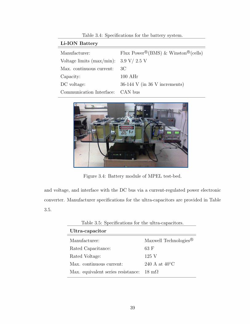
Table 3.4: Specifications for the battery system.
Li-ION Battery
Manufacturer: Flux Power R©(BMS) & Winston R©(cells)
Voltage limits (max/min): 3.9 V/ 2.5 V
Max. continuous current: 3C
Capacity: 100 AHr
DC voltage: 36-144 V (in 36 V increments)
Communication Interface: CAN bus
Figure 3.4: Battery module of MPEL test-bed.
and voltage, and interface with the DC bus via a current-regulated power electronic
converter. Manufacturer specifications for the ultra-capacitors are provided in Table
3.5.
Table 3.5: Specifications for the ultra-capacitors.
Ultra-capacitor
Manufacturer: Maxwell Technologies R©
Rated Capacitance: 63 F
Rated Voltage: 125 V
Max. continuous current: 240 A at 40C
Max. equivalent series resistance: 18 mΩ
39

Figure 3.5: UC module of MPEL test-bed.
3.2 Energy Cycling Capability of Battery and Ultra-capacitor
In this chapter, two sets of experimental results will be presented. The first
experiment demonstrates the energy cycling capabilities when using batteries and
ultra-capacitors, and provides experimental validation for baseline control strategies
to mitigate multi-frequency load fluctuations. The second experiment shows the
energy cycling capability when using the flywheel and ultra-capacitors together in
the AED-HES test-bed.
The experimental setup for the first experiment is shown in Figure 3.6. Power from
the battery and ultra-capacitor modules is used to isolate the power fluctuations from
the DC bus, and the resistive load bank emulates the fluctuating load power, as shown
in Figure 3.7. In this experiment, the 480 VAC power source is converted to a 670V
DC power source by a three-phase diode rectifier, and then a DC/DC converter is
used to buck this voltage down to the desired DC bus voltage of 240V.
The effect of the load fluctuations on the DC bus without regulation is shown
in Figure 3.8. Due to the relatively slow dynamic of the battery, the bus voltage
regulation using batteries alone is only effective in reducing the low frequency distur-
bance. In order to eliminate the high frequency disturbance, bus voltage regulation
using the ultra-capacitor is introduced to assist the battery modules. To exploit the
hybrid configuration of ESDs, two independent voltage regulators using batteries and
40

Figure 3.6: Experimental setup for the energy cycling test using batteries and ultra-capacitors.
time (sec)3160 3170 3180 3190 3200
Pow
er (
W)
0
1000
2000
3000
4000Load Power
Figure 3.7: Multi-frequency load power fluctuations generated by the resistive loadbank.
time (sec)1125 1130 1135 1140 1145
Vol
tage
(V
)
234
236
238
240
242
244
246Reference VbusVbus
Figure 3.8: DC bus voltage without HESS bus voltage regulators.
41

Figure 3.9: Schematic of the independent bus voltage regulation control using bat-teries and ultra-capacitors.
time (sec)2780 2790 2800 2810 2820
Vol
tage
(V
)
234
236
238
240
242
244
246VbusReference Vbus
time (sec)2780 2790 2800 2810 2820
Vol
tage
(V
)
110
120
130
140UC Voltage
Figure 3.10: DC bus voltage with independent bus voltage regulators using batteriesand ultra-capacitors: (a) bus voltage (left) and (b) UC voltage (right).
ultra-capacitors, respectively, are implemented, as shown in Figure 3.9, and the de-
sired DC bus voltage is achieved, as shown in Figure 3.10(a). Note that the solid line
represents the electric power and the dashed line represents the control and feedback
signals. However, regulating the bus voltage using two independent voltage regulators
causes a significant drop in ultra-capacitor voltage (shown in Figure 3.10(b)), leading
to large output current and requiring frequent recharging.
A filter-based control strategy is demonstrated in the next experimental test.
The schematic of the filter-based control strategy is shown in Figure 3.11, where
the battery compensates the low-frequency load fluctuations, and the ultra-capacitor
compensates the high-frequency fluctuations. To deal with uncertainties in the load
information, a bus voltage regulator is integrated with the feedforward portion of
42

Figure 3.11: Schematic of the filter-based control using batteries and ultra-capacitors.
time (sec)2600 2610 2620 2630 2640
Vol
tage
(V
)
234
236
238
240
242
244
246VbusReference Vbus
time (sec)2600 2610 2620 2630 2640
Vol
tage
(V
)
110
120
130
140UC Voltage
Figure 3.12: DC bus voltage with filter-based control using batteries and ultra-capacitors: (a) bus voltage (left) and (b) UC voltage (right).
the ultra-capacitor controller. The DC bus voltage regulation performance and the
ultra-capacitor voltage change are shown in Figure 3.12(a) and (b), respectively. Note
that the only load power in this experiment is from the load resistive bank, which
represents the load fluctuations. Because the batteries and ultra-capacitors isolate
the load fluctuations from the DC bus, the power from the AC power source is almost
zero. Furthermore, the ultra-capacitor voltage change is reduced to 1.88V with the
filter-based baseline control.
These two baseline control strategies demonstrate the energy cycling capability of
the batteries and ultra-capacitors. It is clear from the experimental results for the
baseline control strategies that coordinated control strategies are needed to maximize
the benefits of using HESS.
43

Figure 3.13: Experimental setup for the energy cycling test using the flywheel andultra-capacitors.
Figure 3.14: Schematic of the filter-based control using the flywheel and ultra-capacitors.
3.3 Energy Cycling Capability of Flywheel and Ultra-capacitor
The energy cycling capability of the HESS configuration consisting of the flywheel
and ultra-capacitors is demonstrated in the second experiment, where the flywheel
is used to compensate the low-frequency load fluctuations and the ultra-capacitors
address the high-frequency fluctuations. In this experiment, the rectified 480 VAC
power source is bucked down to 400 V, which is the nominal voltage of the flywheel.
The load fluctuation is again generated by the load resistor bank. The corresponding
experimental setup developed for this test, and the schematic of the control strategy,
are shown in Figures 3.13 and 3.14, respectively. Results are given in Figure 3.15,
44

time (sec)3160 3170 3180 3190 3200
Vol
tage
(V
)
234
236
238
240
242
244
246VbusReference Vbus
time (sec)3160 3170 3180 3190 3200
Vol
tage
(V
)
110
120
130
140
UC Voltage
Figure 3.15: DC bus voltage with filter-based control using the flywheel and ultra-capacitors: (a) bus voltage (left) and (b) UC voltage (right).
which demonstrate the effectiveness of the flywheel and ultra-capacitors to compen-
sate the load fluctuations and to regulate the DC bus voltage at the desired value.
These experimental tests not only demonstrate the energy cycling capability of
the AED-HES test-bed, but also illustrate the importance of the control strategy.
3.4 Summary
This chapter presents the development and experimental demonstration of the
AED-HES test-bed for electric ship propulsion systems at the University of Michigan
Power and Energy Lab. A system-level controller, electric machines, high-power con-
verters, and energy storage devices (batteries, UCs, and flywheel) are integrated in the
AED-HES test-bed. The AED-HES test-bed facilitates efforts to address load fluctua-
tions in propulsion systems, and can be used as an essential tool to evaluate modeling
and control solutions. Two experiments with different energy storage devices are
performed to demonstrate the energy cycling capability of AED-HES testbed. The
experiential validation of advanced control approaches will be presented in Chapter
VIII.
45

CHAPTER IV
Hybrid Energy Storage Configuration Evaluation:
Battery with Flywheel vs. Battery with
Ultracapacitor
This chapter investigates the feasibility and effectiveness of introducing a hybrid
energy storage system (HESS) to an electric propulsion system for mitigating load
power fluctuation effects on a shipboard network. The potential of Battery with Ultra-
capacitor (B/UC) and Battery with Flywheel (B/FW) HESS in counteracting load
fluctuations is formulated as a multi-objective optimization problem (MOP). Two
main objectives are power-fluctuation compensation and HESS loss minimization.
Since these objectives conflict with each other in the sense that effective compensation
of fluctuations will lead to HESS losses, the weighted-sum method is used to convert
this MOP into a single-objective problem. Global optimal solutions are obtained
using dynamic programming (DP) by exploiting the periodicity of the load. These
global optimal solutions form the basis of a comparative study of B/FW and B/UC
HESS, where the Pareto fronts of these two technologies at different sea state (SS)
conditions are derived. The analysis aims to provide insights into the advantages
and limitations of each HESS solution. To enable real-time application and achieve
desired performance, a model predictive control (MPC) strategy is developed. In this
46

MPC formulation, a state of charge (SOC) reference is used to address the limitations
imposed by short predictive horizons.
4.1 Performance Evaluation of B/FW And B/UC HESS Con-
figurations
4.1.1 Problem Formulation
In this study, the control strategies of HESS are designed to achieve two objectives:
one is to minimize the power tracking error, measured by the root mean square (RMS)
error for power fluctuation mitigation, and the other is to reduce HESS losses to
improve energy efficiency:
J1 =
NT∑k=0
(PFL(k)− PHESS(k))2, (4.1)
J2 =
NT∑k=0
(PHESSLoss), (4.2)
where NT = [(tT − t0)/Ts], with [·] being the integer rounding of ·, t0 and tT are the
initial and final values of the time period being investigated, Ts is the sampling time,
PFL is the load power fluctuation from the propeller and ship dynamics model, PHESS
is the power generated by HESS to compensate the load fluctuations, and PHESSLoss
is the HESS losses. Note that the RMS tracking error can be expressed as√J1/NT .
Since NT is constant, minimizing J1 is equivalent to minimizing the RMS tracking
error.
Because J1 and J2 compete in the sense that reducing the tracking error would
cause increased HESS losses and vice versa, the weighted-sum method, which converts
the multi-objective optimization problem (MOP) to a single-objective optimization
problem, is used to find the non-dominated solutions (i.e., Pareto front) in this prob-
lem. The problem formulation of B/FW is expressed as follows. Minimize:
47

JHESSB/FW(x(k), u(k))
=
NT∑k=0
(1− λ)(PFL(k)− PB(k)− PFW (k))2
+ λ
[NBRBu
2B(k) +NFW
(b(ωmaxxFW (k))2 +
3
2Rs
(uFW (k)
34pPMΛFW
)2)]
,
(4.3)
subject to the constraints:
20% ≤ xB ≤ 90%,
30% ≤ xFW ≤ 99%,
−200A ≤ uB ≤ 200A,
−40Nm ≤ uFW ≤ 40Nm,
−90KW ≤ uFWxFWωmax ≤ 90KW,
(4.4)
xB(k + 1)
xFW (k + 1)
=
1 0
0 1− bTs
ωmaxJFW
xB(k)
xFW (k)
+
Ts
3600QB0
0 Ts
ωmaxJFW
uB(k)
uFW (k)
,(4.5)
while the problem formulation for the B/UC HESS is given by:
JHESSB/UC(x(k), u(k)) =
NT∑k=0
(1− λ)(PFL(k)− PB(k)− PUC(k))2
+ λ(NBRBu2B(k) +NUCRUCu
2UC(k)),
(4.6)
48
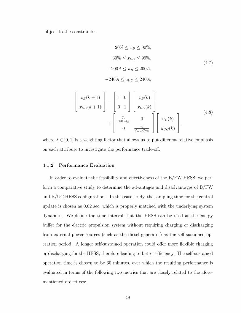
subject to the constraints:
20% ≤ xB ≤ 90%,
30% ≤ xUC ≤ 99%,
−200A ≤ uB ≤ 200A,
−240A ≤ uUC ≤ 240A,
(4.7)
xB(k + 1)
xUC(k + 1)
=
1 0
0 1
xB(k)
xUC(k)
+
Ts
3600QB0
0 Ts
VmaxCUC
uB(k)
uUC(k)
,(4.8)
where λ ∈ [0, 1] is a weighting factor that allows us to put different relative emphasis
on each attribute to investigate the performance trade-off.
4.1.2 Performance Evaluation
In order to evaluate the feasibility and effectiveness of the B/FW HESS, we per-
form a comparative study to determine the advantages and disadvantages of B/FW
and B/UC HESS configurations. In this case study, the sampling time for the control
update is chosen as 0.02 sec, which is properly matched with the underlying system
dynamics. We define the time interval that the HESS can be used as the energy
buffer for the electric propulsion system without requiring charging or discharging
from external power sources (such as the diesel generator) as the self-sustained op-
eration period. A longer self-sustained operation could offer more flexible charging
or discharging for the HESS, therefore leading to better efficiency. The self-sustained
operation time is chosen to be 30 minutes, over which the resulting performance is
evaluated in terms of the following two metrics that are closely related to the afore-
mentioned objectives:
49

0.85 0.9 0.95 1 1.05 1.1 1.15
Loss (%)
0
200
400
600
800
1000
RM
S E
rror
(W
)
SS2 (B/FW vs B/UC)
B/FW Pareto-frontB/UC Pareto-front
RP 1RP 2
Figure 4.1: Pareto-fronts of B/FW and B/UC HESS at sea state 2.
1. RMS tracking error:√J1/NT ;
2. HESS losses: Loss% = J2∑NTk=0 PDemand(k)
× 100%.
The weighting factor λ allows us to put a different relative emphasis on each
attribute to investigate the performance trade-off. The global optimal solutions of
B/FW and B/UC MOPs are obtained by dynamic programming (DP). The Pareto-
fronts of these two configurations, which represent the best achievable performance
for the system with B/FW HESS and B/UC HESS, are shown in Figures 4.1-4.3. The
Pareto fronts provide insight into the effectiveness of HESS and the trade-off between
the tracking RMS error and the HESS losses. The key observations are summarized
in the following remarks:
Remark 4.1 (Performance trade-off features): The tracking performance can be
improved over a wide range at little cost of system efficiency for low and medium
sea states (sea states 2 and 4). This feature can be observed for both B/FW and
B/UC HESS solutions. Furthermore, the general trends and Pareto front shapes are
the same for both HESS configurations at all sea states. In terms of managing the
50

1.05 1.1 1.15 1.2 1.25 1.3
Loss (%)
0
500
1000
1500
2000
RM
S E
rror
(W
)
SS4 (B/FW vs B/UC)
B/FW Pareto-frontB/UC Pareto-front
RP 4 RP 3
Figure 4.2: Pareto-fronts of B/FW and B/UC HESS at sea state 4.
1 1.2 1.4 1.6 1.8 2 2.2 2.4
Loss (%)
0.8
0.9
1
1.1
1.2
1.3
RM
S E
rror
(%
)
105 SS6 (B/FW vs B/UC)
B/FW Pareto-frontB/UC Pareto-front
RP 5
RP 6
RP 8RP 7
Figure 4.3: Pareto-fronts of B/FW and B/UC HESS at sea state 6.
trade-off, they both have the same features and issues.
Remark 4.2 (B/FW vs. B/UC): As shown in Figures 4.1-4.3, the B/FW HESS is
able to achieve superior performance at sea state 6. However, at sea states 2 and 4,
the B/UC HESS achieves better performance than B/FW HESS, but the difference
between B/FW HESS losses and B/UC HESS losses at sea state 2 (around 0.22%)
51

is about twice as large as that at sea state 4 (around 0.11%). Note that the load
power fluctuations at sea state 2 are smaller than those at sea state 4. The analysis
indicates that B/FW HESS is more suitable for the high sea state, while the B/UC
HESS has performance advantages at low sea states.
To reveal more details of the HESS performance, several representative points
(RP) are highlighted in Figures 4.1-4.3 for further analysis. As shown in Figures
4.1-4.2, those points reflect the best trade-off between two objectives and they are
closest to the “utopia” points (J1min, J2min). Therefore, RP1-RP4 are the design
points analyzed here. The RMS tracking errors of these design points, i.e., RP1-RP4,
are almost the same at the same sea state. RP5-RP8 are the points with comparable
performance in one of the attributes at sea state 6. Besides the two main objectives in
Figures 4.1-4.3, several other metrics are used for evaluating these solutions as shown
in Table 4.1:
Table 4.1: Performance metrics.IBRMS
Battery currents measured by the rms (root mean square) value.IBPeak
Battery currents measured by the maximum absolute value.TIB1.5C
% The time spent charging/discharging the battery with high currents:the percentage of high current operation (|IB| ≥ 1.5C).
LossB% Battery conduction loss: LossB% =∑NT
k=0(PowerB−loss(k))∑NTk=0 PDemand(k)
× 100%.
LossUC% Ultra-capacitor conduction loss: LossUC% =∑NT
k=0(PowerUC−loss(k))∑NTk=0 PDemand(k)
×100%.
LossFWRs% Flywheel conduction loss: LossFWRs
% =∑NT
k=0(PowerFWRs−loss(k))∑NTk=0 PDemand(k)
×100%.
LossFWf% Flywheel spinning loss: LossFWf
% =∑NT
k=0(PowerFWf−loss(k))∑NTk=0 PDemand(k)
× 100%.
The metrics IBRMS, IBPeak
and IB1.5C% are used to evaluate the battery usage, as
they have high impact on the battery life; the power losses of each energy storage as
well as the losses due to different mechanisms in the flywheel provide insight into the
operation of HESS. The key observations about the reference points are summarized
in the following remarks:
52

Table 4.2: Performance comparison of the selected design points.RP1 RP2 RP3 RP4 RP5 RP6 RP7 RP8
Sea State 2 2 4 4 6 6 6 6IBRMS
12.13A 17.33A 16.02A 21.51A 51.59A 55.86A 74.96A 95.62AIBPeak
31.48A 52.85A 72.00A 82.00A 200A 200A 200A 200ATIB1.5C
% 0 0 0 0 3.67% 4% 8.50% 19.0%LossB% 0.05% 0.09% 0.07% 0.13% 0.39% 0.46% 0.82% 1.34%LossUC% NA 0.80% NA 0.99% NA 0.75% NA 0.88%LossFWRs
% 0.53% NA 0.48% NA 0.35% NA 0.36% NALossFWf
% 0.54% NA 0.67% NA 0.43% NA 0.44% NA
Remark 4.3 (Battery usage): B/FW HESS is more ‘friendly’ to batteries with
smaller IBRMS, IBPeak
, and less time spent at high-current operation TIB1.5C%, as
shown in Table 4.2. At sea state 2, IBRMSand IBPeak
of the B/UC HESS are almost
twice as large as those of B/FW HESS. At sea state 4, the B/FW HESS requires
less IBRMSand IBPeak
than B/UC to achieve almost the same tracking error. At sea
state 6, RP5 and RP6 have almost the same HESS losses, but RP5 (B/FW) achieves
much smaller power tracking RMS error. B/FW HESS requires less battery usage
and high-current operation, while achieving improved power tracking performance.
For RP7 and RP8, the battery high-current operation for B/UC HESS is even more
than twice that of the B/FW.
Remark 4.4 (Loss analysis): At sea state 2, even though both the battery RMS and
peak current with B/FW are less than those with B/UC, the loss of B/FW is larger
than that of B/UC. The reason for this is that the standby loss of the flywheel, namely
the spinning loss (including core losses and windage losses), is significant at the low sea
state. In particular, the battery needs to discharge more to compensate the spinning
losses of the flywheel in order to keep the flywheel working at its optimal speed.
Therefore, the drag coefficient is the key design parameter of the flywheel, especially
for a high-speed flywheel. At high sea state, the spinning loss of the flywheel is not
the main issue of the B/FW HESS configuration. The high power demand of the
low-frequency load fluctuation requires the HESS to provide or absorb the maximum
power for several seconds. The flywheel working in its high speed range sustains for
53

a longer period of time to generate or absorb the maximum power when compared
to the ultra-capacitor. Therefore, as shown in Table 4.2 and Figure 4.3, B/FW can
outperform B/UC in terms of improved tracking performance, reduced HESS losses,
and extended battery life cycle. Note that some flywheel motor/generators have much
lower spinning core loss (e.g., synchronous reluctance machines), but have lower power
density and full-load efficiency.
Remark 4.5 (Sensitivity to battery aging): It has been widely reported that batter-
ies degrade over their life cycle, as the battery capacity will decrease and the battery
resistance will increase [79]. A sensitivity study is performed to provide insights into
the impact of the battery state of health (SOH) on the proposed HESS solutions.
In this study, SOH is characterized by battery capacity reduction and resistance in-
crease. As shown in Figure 4.4, the increased battery resistance has a more significant
impact on the proposed solutions compared to the decreased battery capacity. The
HESS works as an energy buffer instead of an energy source, as the generator sets
provide the average power for the electric propulsion system. Due to the high energy
density of the battery, the battery SOC variation within the self-sustained time is
very small. Although the degraded capacity can increase the SOC variation, the bat-
tery open circuit voltage VOC(x1) is in general insensitive to this small SOC variation.
Therefore, the impact of the decreased capacity is relatively small. The impact of
increased battery resistance on the B/UC HESS at sea states 2 and 4 is larger than
it is on the B/FW HESS. As discussed in the previous remarks, the spinning losses
of the flywheel is dominant in B/FW HESS at low sea state, as shown in Table 4.2,
whereas the battery resistance, which affects the battery loss, has less of an effect.
However, at high sea state, due to the high-power fluctuations, the battery losses
become more significant even in the B/FW configuration. Therefore, the sensitivity
to battery resistance is noticeable for both B/FW and B/UC HESS.
54

The MOP formulated here can be used to evaluate the effectiveness of different
HESS configurations and analyze their advantages and limitations. However, the
solution of the MOP cannot be used for real-time applications. It is an open-loop
optimization without feedback. Furthermore, this optimization problem has a very
long horizon in the sense that 90,000 steps are involved when the minimum self-
sustained operation time of HESS is chosen to be 30 minutes. This requires a long
computational time and large memory, which makes it computationally prohibitive
to solve in real time, and leads to the MPC formulation discussed in the next section.
4.2 Receding Horizon Control for Real-Time Power Manage-
ment
In this section, the receding-horizon approach is applied to develop a real-time
energy management scheme. To capture the dynamics of HESS and address the
associated operation constraints, MPC emerges as a natural choice. The general
MPC problem, which minimizes a cost function subject to constraints within the
predictive horizon, can be mathematically expressed as:
J = Φ(x(t+N)) +t+N−1∑k=t
L(x(k), u(k)), (4.9)
subject to:
x(k + 1) = f(x(k), u(k)), x(t) = x0, (4.10)
C(x(k), u(k)) ≤ 0, (4.11)
where Φ(x(t + N)) and L(x(k), u(k)) are the terminal and instantaneous cost func-
tions, N is the time window over which the cost will be evaluated, x(k) and u(k)
are the instantaneous values of the states (x ∈ <2) and controls (u ∈ <2) at time k,
respectively, C(x(k), u(k)) represents the inequality constraints, and t represents the
55

0.9 0.95 1 1.05 1.1Loss (%)
0
500
1000
1500
RM
S E
rror
(W
)
SS2 (B/FW vs B/UC)
B/FW (R=R0)
B/UC (R=R0)
B/FW (R=110%R0)
B/UC (R=110%R0)
B/FW (R=120%R0)
B/UC (R=120%R0)
0.85 0.9 0.95 1 1.05 1.1 1.15
Loss (%)
0
500
1000
1500
RM
S E
rror
(W
)
SS2 (B/FW vs B/UC)
B/FW (Q=Q0)
B/UC (Q=Q0)
B/FW (Q=90%Q0)
B/UC (Q=90%Q0)
B/FW (Q=80%Q0)
B/UC (Q=80%Q0)
1.05 1.1 1.15 1.2 1.25 1.3 1.35Loss (%)
0
500
1000
1500
2000
RM
S E
rror
(W
)
SS4 (B/FW vs B/UC)B/FW (R=R
0)
B/UC (R=R0)
B/FW (R=110%R0)
B/UC (R=110%R0)
B/FW (R=120%R0)
B/UC (R=120%R0)
1.05 1.1 1.15 1.2 1.25 1.3 1.35
Loss (%)
0
500
1000
1500
RM
S E
rror
(W
)
SS4 (B/FW vs B/UC)
B/FW (Q=Q0)
B/UC (Q=Q0)
B/FW (Q=90%Q0)
B/UC (Q=90%Q0)
B/FW (Q=80%Q0)
B/UC (Q=80%Q0)
1 1.5 2
Loss (%)
0.8
0.9
1
1.1
1.2
1.3
1.4
RM
S E
rror
(%
)
105 SS6 (B/FW vs B/UC)B/FW (R=R
0)
B/UC (R=R0)
B/FW (R=110%R0)
P/UC (R=110%R0)
B/FW (R=120%R0)
P/UC (R=120%R0)
1 1.5 2
Loss (%)
0.8
0.9
1
1.1
1.2
1.3
1.4
RM
S E
rror
(%
)
105 SS6 (B/FW vs B/UC)
B/FW (Q=Q0)
B/UC (Q=Q0)
B/FW (Q=90%Q0)
B/UC (Q=90%Q0)
B/FW (Q=80%Q0)
B/UC (Q=80%Q0)
Figure 4.4: Pareto-fronts of B/FW and B/UC HESS at sea states 2,4 and 6 withdifferent battery state of health.
current sample time. By minimizing (4.9) subject to (4.10) and (4.11), an optimized
control sequence u∗(t), u∗(t + 1), ..., u∗(t + N − 1) can be obtained. The standard
receding horizon MPC then applies the first element of the sequence as the control
action before moving to the next sample, when new measurements are collected and
the optimization is repeated with new initial conditions [80]-[81].
56

The cost function in MPC is formulated based on the MOP by using the weighted-
sum method. We discretize the system model developed in Chapter II with sampling
time Ts. No terminal cost is incorporated in this MPC formulation. Therefore, the
MPC formulation of B/FW is defined as:
JHESSB/FW=
t+N−1∑k=t
LHESSB/FW(x(k), u(k)), (4.12)
where
LHESSB/FW(x(k), u(k))
= (1− λ)(PFL(k)− PB(k)− PFW (k))2
+ λ
[NBRBu
2B(k) +NFW
(b(ωmaxxFW (k))2 +
3
2Rs
(uFW (k)
34pPMΛFW
)2)]
,
(4.13)
subject to the constraints (4.4) and (4.5), where λ ∈ [0, 1] is the weighting factor
that allows us to put different relative emphasis on each attribute to investigate the
performance trade-off.
The short-horizon MPC, however, cannot incorporate the long-term perspectives
of operation. As a result, we observed that the SOC of the flywheel drops quickly. As
it decreases, delivering the same output power requires larger torque, thereby leading
to significantly increased losses and power tracking error, as shown in Figure 4.5.
To keep the flywheel working in a high-efficiency range without having to extend
the MPC predictive horizon, we analyzed the DP results to help us find mechanisms to
assure long-term system efficiency. The representative point RP3 as shown in Figure
4.2 is used as a benchmark in this section. As shown in Figure 4.6, the B/FW HESS
operation can be divided into three phases: transient, sustaining, and final. Given
different initial SOCs of the flywheel, it converges to the same SOC range, which is
the high-efficiency range for B/FW HESS, during the transient interval. When the
B/FW HESS is operating during the sustaining interval, the battery will keep the
57

0 200 400 600 800 1000 1200 1400 1600 1800-2
0
2
Pow
er (
W) 104
Power Tracking Error
0 200 400 600 800 1000 1200 1400 1600 180078
80
82
SO
C (
%) Battery SOC
0 200 400 600 800 1000 1200 1400 1600 1800
time (sec)
20
40
60
SO
C (
%) Flywheel SOC
Figure 4.5: B/FW HESS performance at sea state 4 without any penalty on the speedof FW.
0 200 400 600 800 1000 1200 1400 1600 1800
time (sec)
48
50
52
54
56
58
60
SO
C (
%)
MOP Dynamic Programming Results
FW SOC (Initial=50%, MOP)FW SOC (Initial=60%, MOP)
SustainingTransient Final
Figure 4.6: The flywheel SOC of MOP dynamic programming solutions with differentinitial SOCs.
flywheel SOC in its high-efficiency range to minimize the cost in (4.3). During the
final interval, the battery is not required to maintain the flywheel SOC, and so the
flywheel will be used as much as possible. In order to maximize the benefits of B/FW
HESS, a long self-sustained time is preferred, which requires that the flywheel works
in its high-efficiency SOC range. This observation motivates us to add another term
58

into the cost function with a penalty on the SOC deviations from the optimal settings
(4.3):
γFWSOC(xFW (k)− SOCFWd
)2, (4.14)
The cost function used in the MPC optimization formulation then has the form:
LHESSB/FW(x(k), u(k))
= (1− λ)(PFL(k)− PB(k)− PFW (k))2
+ λ
[NBRBu
2B(k) +NFW
(b(ωmaxxFW (k))2 +
3
2Rs
(uFW (k)
34pPMΛFW
)2)]
+ γFWSOC(xFW (k)− SOCFWd
)2;
(4.15)
Increasing γ initially improves the performance, but further increases in γ beyond
a certain value will lead to deteriorated performance. The reason is that, when
initially increasing γ, the flywheel can operate around its optimal SOC, leading to
improved efficiency. However, if γ is too large, then the flywheel is forced to operate
close to its optimal SOC with small variations, which leaves most of the compensation
function on the batteries. That makes the HESS function essentially a battery energy
storage system, thereby losing the advantage of the hybrid configuration. By varying
γ, we are able to obtain the best achievable solution. In this study, γ is tuned off-line.
Note that how to obtain the optimal reference SOC is an open question, and will be
explored in future work.
The performance of the proposed MPC energy management strategy and DP is
shown in Figure 4.7. As shown in the zoom-in plots of Figure 4.7, the flywheel
SOC under the proposed MPC can achieve the same trajectory as DP during the
sustaining interval. The battery output current and flywheel output torque of MPC
and DP are also almost the same, thereby achieving almost equivalent performance.
59
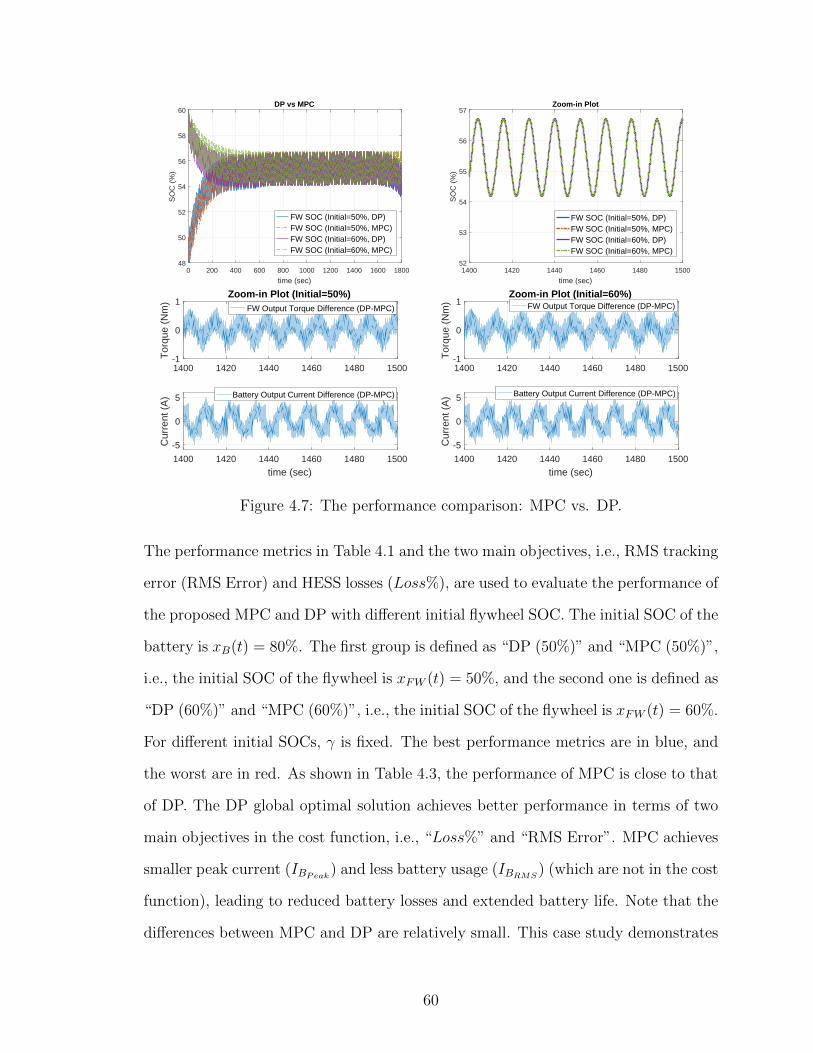
0 200 400 600 800 1000 1200 1400 1600 1800
time (sec)
48
50
52
54
56
58
60
SO
C (
%)
DP vs MPC
FW SOC (Initial=50%, DP)FW SOC (Initial=50%, MPC)FW SOC (Initial=60%, DP)FW SOC (Initial=60%, MPC)
1400 1420 1440 1460 1480 1500
time (sec)
52
53
54
55
56
57
SO
C (
%)
Zoom-in Plot
FW SOC (Initial=50%, DP)FW SOC (Initial=50%, MPC)FW SOC (Initial=60%, DP)FW SOC (Initial=60%, MPC)
1400 1420 1440 1460 1480 1500-1
0
1
Tor
que
(Nm
)
Zoom-in Plot (Initial=50%)FW Output Torque Difference (DP-MPC)
1400 1420 1440 1460 1480 1500
time (sec)
-5
0
5
Cur
rent
(A
) Battery Output Current Difference (DP-MPC)
1400 1420 1440 1460 1480 1500-1
0
1
Tor
que
(Nm
)
Zoom-in Plot (Initial=60%)FW Output Torque Difference (DP-MPC)
1400 1420 1440 1460 1480 1500
time (sec)
-5
0
5
Cur
rent
(A
) Battery Output Current Difference (DP-MPC)
Figure 4.7: The performance comparison: MPC vs. DP.
The performance metrics in Table 4.1 and the two main objectives, i.e., RMS tracking
error (RMS Error) and HESS losses (Loss%), are used to evaluate the performance of
the proposed MPC and DP with different initial flywheel SOC. The initial SOC of the
battery is xB(t) = 80%. The first group is defined as “DP (50%)” and “MPC (50%)”,
i.e., the initial SOC of the flywheel is xFW (t) = 50%, and the second one is defined as
“DP (60%)” and “MPC (60%)”, i.e., the initial SOC of the flywheel is xFW (t) = 60%.
For different initial SOCs, γ is fixed. The best performance metrics are in blue, and
the worst are in red. As shown in Table 4.3, the performance of MPC is close to that
of DP. The DP global optimal solution achieves better performance in terms of two
main objectives in the cost function, i.e., “Loss%” and “RMS Error”. MPC achieves
smaller peak current (IBPeak) and less battery usage (IBRMS
) (which are not in the cost
function), leading to reduced battery losses and extended battery life. Note that the
differences between MPC and DP are relatively small. This case study demonstrates
60

Table 4.3: Performance comparison of the proposed MPC and DP.DP (50%) MPC (50%) DP (60%) MPC (60%)
IBRMS16.75A 16.25A 15.57A 14.81A
IBPeak101A 101A 66.48A 60.4A
IB1.5C% 0 0 0 0
LossB% 0.08% 0.08% 0.07% 0.06%LossFWRs
% 0.48% 0.49% 0.48% 0.48%LossFWf
% 0.67% 0.67% 0.67% 0.69%
Loss% 1.23% 1.24% 1.22% 1.23%RMS Error 153.39W 197.54W 148.57W 179.63W
the effectiveness of the proposed MPC in terms of power-fluctuation compensation,
HESS energy saving, and reduction of the battery usage; in particular, high-current
operation.
The proposed MPC can be easily and effectively extended to the B/UC HESS
solution. As shown in Figure 4.8, without the SOC penalty of UC, the short-horizon
MPC is not able to maintain the UC operating in its high SOC range, because the
benefit of maintaining it is too small in the short term and is therefore ignored in
the optimization. As a result, the SOC of the UC drops quickly. As it decreases,
the delivery of the same output power requires a larger current, thereby leading to
significantly increased losses and power tracking error.
Therefore, to keep the UC working in a high efficiency range, another penalty on
the UC SOC is considered for B/UC HESS:
γUCSOC(xUC(k)− SOCUCd
)2, (4.16)
With this SOC penalty, the UC supplies or absorbs as much power as possible,
and the battery charges the UC to maintain its operation in a high SOC range. The
effectiveness of this γUCSOCpenalty is demonstrated by Figure 4.9.
61

0 500 1000 1500
Pow
er (
W) ×104
-1
0
1
Power tracking error
0 500 1000 1500
Cur
rent
(A
)
-200
0
200 Current of Battery
time(sec)0 500 1000 1500
Cur
rent
(A
)
-2000
200Current of UC
0 200 400 600 800 1000 1200 1400 1600 1800
SO
C (
%)
78.5
79
79.5
80
80.5SOC of Battery
time (sec)0 200 400 600 800 1000 1200 1400 1600 1800
SO
C (
%)
60
80
100SOC of UC
Figure 4.8: MPC (N=20, without UC SOC penalty) performance at sea state 4.
0 500 1000 1500
Pow
er (
W) ×104
-1
0
1 Power tracking error
0 500 1000 1500
Cur
rent
(A
)
-200
0
200 Current of Battery
time(sec)0 500 1000 1500
Cur
rent
(A
)
-2000
200Current of UC
0 200 400 600 800 1000 1200 1400 1600 1800
SO
C (
%)
78.5
79
79.5
80
80.5SOC of Battery
time (sec)0 200 400 600 800 1000 1200 1400 1600 1800
SO
C (
%)
60
80
100
SOC of UC
Figure 4.9: MPC (N=20, with UC SOC penalty) performance at sea state 4.
4.3 Summary
This chapter investigates the feasibility and effectiveness of different HESS con-
figurations, namely batteries combined with flywheels and batteries combined with
UCs, to mitigate load fluctuations. A comparative study is performed to provide
insights into advantages and limitations of each configuration. A multi-objective op-
timization problem (MOP) is formulated to minimize the power tracking error and
HESS losses. The best achievable solutions, namely Pareto fronts, are obtained by
using dynamic programming. The comparison results indicate that the B/FW HESS
configuration outperforms B/UC HESS at high sea state in terms of power fluctu-
ation compensation and HESS efficiency. However, the spinning loss of the B/FW
62

HESS configuration will cause more losses at low sea state, which makes B/UC HESS
configuration more suitable in these conditions. Furthermore, B/FW HESS is more
“friendly” to batteries in terms of less battery usage, reduced peak current, and less
high-current operation for batteries.
In this chapter, in order to enable the real-time implementation, a model predictive
control algorithm is formulated to minimize the tracking RMS error and HESS losses
for B/FW HESS. In order to overcome the limitations caused by the short predictive
horizon of MPC, an additional penalty on the flywheel SOC is introduced to keep
it working in the high-efficiency operation range. The comparison results of MPC
and MOP demonstrate the effectiveness of the proposed MPC in terms of power-
fluctuation compensation, HESS energy saving, and reduction of the battery usage
and high-current operation. The proposed MPC can be easily and effectively extended
to B/UC HESS in the way that an additional penalty on the SOC of UC is required.
63

CHAPTER V
Control Strategies Evaluation: Coordinated
Control vs. Pre-filtered Control
In this chapter, we consider an HESS consisting of batteries and ultra-capacitors,
and explore two control strategies with different levels of coordination among the
HESS elements. The first approach decomposes the power command that is needed to
counteract the fluctuation according to frequency range, and then controls the battery
packs and ultra-capacitor banks independently. This approach will be referred to as
control with pre-filtering (PF) in this chapter. In this case, the charging/discharging
of the two components in HESS are optimized separately so that the ultra-capacitors
handle high-frequency fluctuations, while the batteries handle low-frequency varia-
tions. The other approach, referred to as coordinated control (CC), treats the batter-
ies and ultra-capacitors as a single entity and coordinates their charging/discharging
to counteract the total load fluctuation through an optimization algorithm. The goal
of this study is to quantify the performance difference and understand the critical
roles of a control strategy in HESS implementation. In pursuing this goal, this study
aims to provide insights into the trade-off between performance and control complex-
ity. It should be noted that, while the PF leads to a relatively simple low-dimensional
optimization problem, the CC is expected to offer improved performance. To charac-
terize the performance of HESS, the performance of a single type of energy storage
64

Figure 5.1: Control strategy diagram: left: PF-MPC, right: CC-MPC.
will be included in this study as a benchmark.
5.1 MPC Problem Formulation
In this section, we apply the receding-horizon approach to develop a real-time
energy management scheme that incorporates feedback and is amenable for real-
time computation. Given the nature of the energy storage system, as well as the
operating constraints involved, MPC becomes the natural formulation. Because of the
distinctive frequency components in the load power fluctuation PFL, and the different
dynamic responses of the battery and UC, two ways of structuring the MPC problem
are considered, as illustrated in Figure 5.1. One is control with pre-filtering, where
the charging/discharging of UC and battery modules are optimized such that the UC
power PUC counteracts high-frequency fluctuations PFL−High while the battery power
PB deals with low-frequency variations PFL−Low. PFL−High and PFL−Low refer to the
high-and low-frequency components in PFL, respectively. The other, referred to as
coordinated control, coordinates the charging/discharging of the battery together with
UC to optimize the power split between them to deal with the total power fluctuation.
Similar to MOP, the uncertainties in PFL are not taken into consideration.
65

The cost function in MPC is formulated based on the minimization of RMS track-
ing error and HESS losses. We discretize the system model developed in Chapter II
with the sampling time Ts. No terminal cost is incorporated in this MPC formulation.
As discussed in Chapter IV, the SOC penalty γUCSOCin Equation (4.16) can effec-
tively improve the system performance by ensuring that the UC is operating in its
high-efficiency range. Therefore, the specific variables and functions in the CC-MPC
formulation are defined as:
JHESS =t+N−1∑k=t
LHESS(x(k), u(k)), (5.1)
where,
LHESS(x(k), u(k)) =λTracking(PFL(k)− PB(k)− PUC(k))2
+ λLoss(NBRBu2B(k) +NUCRUCu
2UC(k))
+ γUCSOC(xUC(k)− SOCUCd
)2;
(5.2)
subject to the same constraints in Equations (4.7) and (4.8), and u = [uB, uUC ],
where λTracking, λLoss, and γUCSOCare the weights on power tracking error penalty,
the energy loss penalty, and UC SOC charging penalty, respectively.
In the PF strategy, the batteries compensate low-frequency fluctuations and UCs
compensate high-frequency fluctuations. As shown in Figure 2.3 of Chapter II, the
high-frequency component in the load power fluctuation frequency spectrum is around
8Hz, while the low-frequency components are smaller than 1Hz. A second-order
butterworth low-pass filter, whose cutoff frequency is set at 1Hz, is used to split
the HESS power demand PFL into high (PFL−High) and low-frequency (PFL−Low)
components. Since both batteries and UCs are subject to constraints in (4.7), MPC
will also be used in the PF strategy. The two separate MPC problems are defined for
PF as:
MPC-B:
66

JB =t+N−1∑k=t
LB(xB(k), uB(k)), (5.3)
where,
LB(uB(k)) =λTracking(PFL−Low(k)− PB(k))2
+ λLoss(NBRBu2B(k)),
(5.4)
subject to constraints related to battery in (4.7)-(4.8); and
MPC-UC:
JUC =t+N−1∑k=t
LUC(xUC(k), uUC(k)), (5.5)
where,
LUC(x2(k), u2(k)) =λTracking(PFL−High(k)− PUC(k))2
+ λLoss(NUCRUCu2UC(k))
+ γUCSOC(xUC(k)− SOCUCd
)2,
(5.6)
also subject to constraints related to UC in (4.7)-(4.8).
To quantify the improvement in the HESS system performance, we also formulate
the MPC problem for a system where only ultracapacitors are used. Because there is
no battery to maintain the UC at a high SOC level, the penalty in Equation (4.16)
is not included, which prevents the occurrence of an extremely large error on power
tracking. Therefore, for the “UC only” configuration (UC-Only), the MPC problem
is defined as:
JUCOnly =t+N−1∑k=t
LUCOnly(x(k), u(k)), (5.7)
where,
LUCOnly(xUC(k), uUC(k)) =λTracking(PFL(k)− PUC(k))2
+ λLoss(NUCRUCu2UC(k)),
(5.8)
subject to the constraints related to UC in (4.7) and (4.8).
67

Note that NUC for the HESS configuration is 9, and for the “UC only” configura-
tion, it is 14.
5.2 Performance Comparison and Results Analysis
With the models built in Chapter II and the HESS components determined above,
we present a case study for quantifying the effects of different control strategies on
the electric drive system with HESS. In the case study, the sampling time for the
control update is chosen as 0.02 sec, which is properly matched with the underlying
system dynamics. The self-sustained operation period is defined as the continuous
time that the HESS can be used as the energy buffer for the electric propulsion system
without requiring charging or discharging from external power sources (such as the
diesel generator). This is determined to be 40 minutes for SS4 and 30 minutes for
SS6. The generator will slowly charge the battery to the initial SOC after 40 minutes
of continuous operation at SS4, and 30 minutes at SS6. The optimization problem
is solved by sequential quadratic programming (SQP). The resulting performance is
evaluated in terms of the following two metrics:
1. RMS tracking error:√J1/NT ;
2. HESS losses: Loss% = J2∑NTk=0 PDemand(k)
× 100%.
Two case studies are performed in the following subsections. In the first case study,
the rotational speed is assumed as constant, which means that the load torque is fully
balanced by the motor torque. This gives us the worst-case scenario in terms of the
mechanical power fluctuations being transferred to the electrical system. We focus
on this worst case first since an attempt will be made to balance the motor torque
given that ‘the torque imbalance is responsible for the propeller wear and tear’, as
discussed in Section 5.5.5 of [20]. In the second case study, where the rotational speed
is regulated by a PI controller, the filter effect of the propeller is considered.
68

Loss (%)0 1 2 3 4 5
RM
S E
rror
(W
)
×104
0
0.5
1
1.5
2Sea State 4
UC OnlyCC-MPC (HESS)PF-MPC (HESS)
Figure 5.2: Pareto-fronts of UC-Only, CC-MPC and PF-MPC at sea state 4 (N=20).
5.2.1 Case I: Constant Propeller Rotational Speed
The weighting factors allow us to put different emphasis on each attribute to
investigate the performance trade-off. By varying λTracking, λLoss and γUCSOC, the
UC-Only (5.7), the PF-MPC (5.3)-(5.5) and the CC-MPC (5.1) problems are solved
at sea states 4 and 6. The Pareto-fronts of these three solutions, which represent the
best achievable system performance with HESS and only ultra-capacitors, are shown
in Figures 5.2-5.3 with the predictive horizon N = 20. The results indicate that the
CC-MPC has substantial advantages over the PF-MPC and UC-Only configurations
in terms of mitigating the load power fluctuations and reducing losses at both sea
states 4 and 6. Note that the constraints are not active in these simulation results.
However, after a long self-sustained operation period, the SOC constraint of the
battery will become active. MPC is able to guarantee the battery working within
these constraints. If the performance is degraded, the HESS can be recharged before
the battery reaches its constraints.
The key observations are summarized in the following remarks:
Remark 5.1: The Pareto-fronts give insight into the effectiveness of HESS with
69

Loss (%)0.5 1 1.5 2 2.5 3 3.5 4
RM
S E
rror
(W
)
×105
1
1.5
2
2.5
Sea State 6UC OnlyCC-MPC (HESS)PF-MPC (HESS)
Figure 5.3: Pareto-fronts of UC-Only, CC-MPC and PF-MPC at sea state 6 (N=20).
MPC and the trade-off between the tracking RMS error and the HESS losses. As
shown in Figures 5.2-5.3, the CC-MPC strategy has substantial advantages with
regard to tracking error mitigation compared with the energy storage system with
only ultra-capacitors. Furthermore, the CC-MPC strategy can reduce the tracking
RMS error without significant increase in losses at sea states 4 and 6 compared with
the PF-MPC strategy.
Remark 5.2: A proper control strategy is critical for capitalizing on the benefits
of HESS. As can be seen from Figures 5.2 and 5.3, UC can do as well as (and even
better than) the HESS if PF-MPC is used. Without proper coordination, the HESS
does not have a convincing performance advantage.
Remark 5.3: Under coordinated control, the battery will properly charge the
UC to keep it working in an efficient operating range to achieve a desired tracking
performance with high efficiency, as shown in Figure 5.4 (a). In contrast, without
coordination, the UC cannot assist the battery to reduce the losses, and the battery
cannot properly charge the UC when needed, leading to a shortened self-sustained
operation time and degraded performance, as shown in Figure 5.4 (b). Compared to
70

0 200 400 600 800 1000 1200 1400 1600 1800P
ower
(W
)-4000
0
4000
8000(a) CC-MPC
Power tracking error
0 200 400 600 800 1000 1200 1400 1600 1800
SO
C (
%)
76
78
80
82SOC of Battery
time (sec)0 200 400 600 800 1000 1200 1400 1600 1800
SO
C (
%)
85
90
95
SOC of UC
0 200 400 600 800 1000 1200 1400 1600 1800
Pow
er (
W)
-4000
0
4000
8000(b) PF-MPC
Power tracking error
0 200 400 600 800 1000 1200 1400 1600 1800
SO
C (
%)
76
78
80
82SOC of Battery
time (sec)0 200 400 600 800 1000 1200 1400 1600 1800
SO
C (
%)
85
90
95
SOC of UC
204 206 208 210 212 214 216
Cur
rent
(A
)
-200
0
200(c) CC-MPC HESS Current (Zoom In)
Current of Battery
time(sec)204 206 208 210 212 214 216
Cur
rent
(A
)
-200
0
200Current of UC
204 206 208 210 212 214 216
Cur
rent
(A
)
-200
0
200(d) PF-MPC HESS Current (Zoom In)
Current of Battery
time(sec)204 206 208 210 212 214 216
Cur
rent
(A
)
-200
0
200Current of UC
Figure 5.4: CC-MPC and PF-MPC performance at sea state 4.
the UC SOC result in Figure 5.4 (b), Figure 5.4 (a) shows a large variation of the SOC
of the UC. This is because the UC in the CC-MPC compensates both high- and low-
frequency fluctuations, but the UC in the PF-MPC compensates only high-frequency
fluctuations. Therefore, the UC in the CC-MPC is used more efficiently than it is in
the PF-MPC. Furthermore, the high-frequency fluctuations in the PF-MPC cannot
be cancelled out or reduced to the level achieved by CC-MPC, as shown in Figure 5.4
(a), because of the penalty of the UC SOC in (5.6). Without this penalty, the UC
SOC in PF-MPC will decrease quickly, and the tracking performance will deteriorate.
Moreover, only when the UC is operating at high current levels will the batteries in
the CC-MPC strategy start to work to assist in reducing the power tracking error and
minimizing the losses, as shown in Figure 5.4 (c). With pre-filtering, however, the
battery and UC can be working at cross purposes; namely, when one is charging the
71

Loss (%)1.15 1.2 1.25 1.3
RM
S E
rror
(W
)
0
1000
2000
3000
4000
5000
6000CC-MPC-N5CC-MPC-N10CC-MPC-N15CC-MPC-N20
Figure 5.5: Sensitivity analysis of predictive horizon for CC-MPC at sea state 4.
other may be discharging. This causes additional losses and degrades power tracking
performance, as shown in Figure 5.4 (d). Consequently, the overall energy consumed
in the PF-MPC, as shown in Figure 5.4 (b), is much more than that in the CC-MPC
shown in Figure 5.4 (a).
Remark 5.4: Extending the predictive horizon will generally improve performance,
at the cost of increased computational complexity. To make the proposed solution
feasible for real-time implementation, a short predictive horizon is used. A sensitivity
analysis of the predictive horizon for CC-MPC is performed to gain insights into
the trade-offs between these design attributes. As shown in Figures 5.5 and 5.6,
the performance is relatively insensitive to the predictive horizon for this problem.
Given that the required computation time depends on not only the algorithm but
also the computation hardware, the work in this section does not directly prove real-
time feasibility. Nevertheless, by providing evidence that a long prediction horizon is
not needed for this problem, it provides strong support that an MPC-based solution
can be practical. Moreover, this sensitivity analysis provides insight that can help
designers manage the trade-off between performance and control complexity.
72

Loss (%)1 1.5 2 2.5 3
RM
S E
rror
(W
)
×105
1
1.1
1.2
1.3
1.4
1.5CC-MPC-N5CC-MPC-N10CC-MPC-N15CC-MPC-N20
Figure 5.6: Sensitivity analysis of predictive horizon for CC-MPC at sea state 6.
5.2.2 Case II: Regulated Propeller Rotational Speed by a PI Controller
In order to consider the filter effect of the ship propeller, another case study is
performed where the rotational speed of the propeller is regulated by a PI controller.
The PI controller for the speed regulation is developed and tuned based on the algo-
rithm given in Appendix B.1 in [19]: KP = 1a
IsTsum
and KI = KP/Ti, where a=3 is a
constant related to the damping ratio, Is = 4800kgm2 is the total propeller rotational
inertia, Tsum = 0.011sec is the lumped time constant of the motor and the shaft speed
sensor filter, and Ti = 0.1sec is the PID controller integral time constant. Since the
high-frequency fluctuations are significantly filtered in Case II, batteries instead of
ultra-capacitors are used as the single type of energy storage. The number of battery
modules is set at 18, as shown in Table 2.4. This “battery only” configuration is
defined as “B-Only” in this case study.
The Pareto-fronts of Case I and II are shown in Figure 5.7 and 5.8. The key
observations are summarized in Remark 5.5.
Remark 5.5: As shown in Figure 5.7 and 5.8, the performance of PF-MPC in
Case II is even worse than that in Case I. The reason for this can be explained
73

Loss (%)0 1 2 3 4 5 6
RM
S E
rror
(W
)
×104
0
0.5
1
1.5
2Sea State 4
CC-MPC (Case I)PF-MPC (Case I)CC-MPC (Case II)PF-MPC (Case II)B-Only (Case II)
Figure 5.7: Pareto-fronts of Case I and II at sea state 4 (N=20).
Loss (%)0.5 1 1.5 2 2.5 3 3.5 4
RM
S E
rror
(W
)
×105
1
1.5
2
2.5
3Sea State 6
CC-MPC (Case I)PF-MPC (Case I)CC-MPC (Case II)PF-MPC (Case II)B-Only (Case II)
Figure 5.8: Pareto-fronts of Case I and II at sea state 6 (N=20).
as follows: The high-frequency power fluctuation in Case II is around 40% of that
in Case I, due to the low-pass filter effect of the inertia and the speed controller
in Case II. However, the low-frequency power fluctuations are almost the same,
which means the battery losses∑N
k=0(Powerbattery−loss(k)) are almost the same un-
der the PF-MPC strategy. Because the losses of batteries are dominant among the
total losses∑N
k=0(Powerbattery−loss(k) + PowerUC−loss(k)), the performance metric
74

204 206 208 210 212 214 216
Cur
rent
(A
)
-200
0
200CC-MPC HESS Current (Case II)
Current of Battery
time(sec)204 206 208 210 212 214 216
Cur
rent
(A
)
-200
0
200
Current of UC
Figure 5.9: The HESS output currents of CC-MPC (Case II) at sea state 4.
Loss% =∑N
k=0(Powerbattery−loss(k)+PowerUC−loss(k))∑Nk=0 |PDemand(k)| × 100% gets worse as the total com-
mand power decreases. On the other hand, the performance of CC-MPC in Case
II is better than that in Case I at sea states 4 and 6, as UCs with CC-MPC not
only cancel out the high-frequency fluctuations but also help in dealing with the low-
frequency fluctuations, as shown in Figure 5.9. As can be seen, the output currents
of batteries and UCs are both reduced, as shown in Figure 5.9, compared to Figure
5.4(d), which indicates that the total HESS losses are significantly reduced and the
battery life is extended. Compared to B-Only in Figure 5.7 and 5.8, CC-MPC out-
performs B-Only at both sea states 4 and 6. This result provides the insight that,
even though the high-frequency fluctuations are significantly filtered, with a proper
strategy, UC is still essential to improve performance in terms of minimizing track-
ing error and losses. In summary, Case II also demonstrates the effectiveness of the
proposed strategy CC-MPC under more realistic conditions.
75

5.3 Summary
In this chapter, control strategies with different levels of coordination among the
HESS elements are studied, and the importance of the coordination is demonstrated.
Due to the frequency characteristics of the power fluctuations, coordinated control
(CC) and pre-filtering (PF) control strategies are investigated. A model predictive
control is formulated based on the multi-objective optimization problem to minimize
the tracking RMS error and HESS losses. A single type of energy storage is also
studied to provide a benchmark in characterizing the performance of HESS. For the
control strategy of HESS, two MPC-based strategies, CC-MPC and PF-MPC, are
designed and evaluated. The comparison results indicate that the CC-MPC strategy
outperforms the PF-MPC strategy in terms of power tracking, HESS efficiency, and
self-sustained operation time. The sensitivity analysis of the predictive horizon for
the coordinated control shows the feasibility of the MPC-based strategies for real-time
applications. In summary, coordinated control is preferred to mitigate the shipboard
load power fluctuations with HESS, given its superior performance and ability in
trading off between achieving power tracking and reducing energy losses.
This study establishes a foundation for pushing HESS technology forward. The
controllers of the generator sets, motor and other components in the electrical propul-
sion have not been taken into consideration in this chapter. The interaction analysis
and energy management strategy design and evaluation for the HESS integrated with
the existing electrical propulsion system will be presented in the next chapter.
76

CHAPTER VI
Energy Management Strategies for An Electric
Ship Propulsion System with Hybrid Energy
Storage
The integration and operation of a shipboard electrical propulsion system with
HESS relies on well-configured HESS hardware and effective power/energy manage-
ment strategies in order to mitigate the load power fluctuation effects and achieve
the desired benefits of increased system efficiency, improved reliability, and reduced
wear and tear. When the HESS is introduced into the existing shipboard electri-
cal propulsion system, it will interact with the generator control systems. Without
proper coordination, the HESS system and the generator control system could inter-
fere with each other, thereby defeating the purposes of HESS. In [19], the widely used
voltage regulator is applied to battery packs to regulate the DC bus voltage, in order
to support the propulsion power. The PI controller is used in [41] for UC to deal with
the pulse power load, leading to system efficiency improvement. In [49], the batteries
and UC work with generators to follow the load profile and reduce fuel consumption.
These control strategies are used to accommodate step or pulse changes in load power,
which differ from the propulsion load fluctuations caused by the hydrodynamic in-
teractions and wave excitations. To the best knowledge of the author, the special
77

challenges associated with the multi-frequency characteristics of the propulsion load
fluctuations and HESS control, as well as the interactions between the HESS control
and primary power generation control systems in dealing with dynamic load fluctua-
tions, have not been well addressed. To address this problem, four control strategies
are studied and analyzed in the first section.
In order to develop a proper control strategy, there are two ways to integrate a new
HESS with the existing propulsion system. One is defined as a ‘plug-in configuration’,
i.e., the new HESS controller works by itself without active coordination with the
existing propulsion system. The other is defined as ‘integrated configuration’, in which
a new integrated controller is developed for the whole propulsion system, including
HESS, propulsion motor, and other power generation systems. In this chapter, energy
management strategies for both plug-in and integrated configurations are studied and
analyzed. The HESS studied in this chapter is based on the B/UC HESS in Chapter
V; i.e., six battery modules and nine UC modules. Similar analysis can be extended
to a battery with flywheel HESS.
6.1 Energy Management Strategies for the Plug-in Configu-
ration
The HESS needs to work with existing control systems in the shipboard power
network in order to achieve the expected benefits of efficiency and reliability improve-
ment. To understand the benefits and limitations of different control designs, four
strategies are investigated in this section, as described in Table 6.1. The general
diagram of the system that embodies these different strategies is shown in Figure 6.1.
78

Table 6.1: Properties of control strategies.
Strategies Properties
1. Baseline System (BL) without HESS Generator control only, HESS is discon-nected.
2. Motor Load Following (MLF) withHESS
HESS control is based on the motor loadinformation, the bus voltage and motorpower information is not used.
3. Bus Voltage Regulation (BVR) withHESS
HESS control is based on the bus volt-age information, the information about themotor load and motor power is not used.
4. Coordinated Energy ManagementSystem (EMS) with HESS
HESS control is based on system informa-tion, including the bus voltage, generatoroutput power, motor input power, and mo-tor load power.
Figure 6.1: Schematic of the electric propulsion system with HESS control strategiesfor the comparative study.
6.1.1 Baseline Control System without HESS
In the baseline (BL) case, a propulsion motor is controlled by a load-following
strategy, and a PI bus voltage regulator is used as the generator control. Without
the HESS, the response of the baseline system serves as a benchmark to evaluate the
benefits or drawbacks of the other strategies. The PI voltage regulator with anti-
windup for the generator control has been successfully used in marine applications
[19, 82]. In this section, the same PI voltage regulator for the generator control is used
for the BL system, as well as for the other three control strategies, when evaluating
79

the performance of each strategy.
To simplify the control system, linearized models are developed around an oper-
ating point. The block diagram of the feedback system for BL is shown in Figure
6.2, where GGen, GBus, and GIM are the transfer functions for the generator with
its rectifier, DC bus, and induction motor with its drive, respectively. The current
changes in the induction motor (IM) caused by the load fluctuation are treated as a
disturbance on the bus. The overall system response, treating the desired bus volt-
age Vd and the load fluctuation LF as the external inputs and the bus voltage error
EDC = Vd − xDC as the performance variable, can be characterized as follows:
EDC =1
1 +GGenGBus
Vd +GIMGBus
1 +GGenGBus
LF. (6.1)
The time response of the baseline system is shown in Figure 6.3. Note that all the
simulation results presented herein are implemented at Sea State 4 and the average
ship speed is 12.4 knots.
Figure 6.2: The block diagram of the feedback system with the baseline strategy.
6.1.2 Motor Load Following Control with HESS
The motor load-following (MLF) strategy for HESS has been explored in many
power and energy applications, such as hybrid electric vehicles. This strategy often
exploits a given load profile or a predictive model. In this section, it utilizes the
motor load information to develop HESS energy management and achieve the optimal
80

475 480 485 490 495 5004120
4130
4140
4150
4160
4170
4180
4190
4200
time [sec]
[V]
BL: Bus Voltage
Figure 6.3: The bus voltage response with the baseline strategy at sea state 4.
performance. However, as shown in Figure 6.4, while HESS control reduces the low
frequency content on the DC bus, it generates more high frequency fluctuations,
leading to deteriorated performance. At a high sea state when the low frequency
disturbance is dominant, as shown in Figure 2.3, this strategy could be effective.
Unfortunately, at a low sea state it will result in a performance that is even worse
than that of the baseline, due to the interaction and the lack of coordination between
the voltage regulation loop and load following loop.
To understand and explain the responses shown in Figure 6.4, a model-based
analysis is performed. To simplify the analysis, the HESS is assumed to follow the
load fluctuation command without tracking error. The block diagram of the simplified
feedback system for MLF is shown in Figure 6.5, whose bus error dynamics can be
described by:
EDC =1
1 +GGenGBus
Vd +(GIM − 1)GBus
1 +GGenGBus
LF. (6.2)
Compared with Equation (6.1), MLF does not influence the system sensitivity
function, which represents the dynamic relationship from the command to the output
81

475 480 485 490 495 500 505 510 515 520 5254120
4140
4160
4180
4200
time [sec]
[V]
BL:Bus VoltageMLF:Bus Voltage
0 2 4 6 8 10 12 14 16 180
2
4
6
Frequency [Hz]
[V]
BL:Bus Voltage VariationMLF:Bus Voltage Variation
BL MLF
Figure 6.4: Performance comparison of BL and MLF: bus voltage response (top plots)and their frequency spectrums (bottom plots) at sea state 4.
error. However, the disturbance transfer function, namely from the load fluctuation
to output error, differs from that of the BL strategy. As shown in Figure 6.6, the
bus voltage variation is significantly reduced at low frequencies, compared to BL, but
noticeably increased at high frequencies, which explains the dynamic behavior shown
in Figure 6.4. The result can be attributed to the fact that this strategy does not take
the motor dynamics and the generator dynamics into consideration in HESS energy
management. It uses only the load information and ignores some system information
(especially the DC bus information), and therefore works independently from the
generator control.
6.1.3 Bus Voltage Regulation with HESS
Bus voltage regulation (BVR) is one of the most widely used control strategies
for energy storage systems, especially in uninterruptible power supply (UPS) applica-
tions. It is a simple control architecture (voltage measurement and feedback) which
aims to stabilize the bus voltage. When HESS is introduced, BVR is a natural choice
82

Figure 6.5: The block diagram of the feedback system with the MLF strategy.
Figure 6.6: Bode plot of load fluctuation response (LF → EDC) by BL and MLF.
for controlling the energy storage to reduce the bus voltage fluctuation caused by
power and thrust variations on the electric drive. Here two PI controllers are used
for batteries and UCs, as expressed in the following:
IB = (KPb+KIb/s)× (Vd − xDC),
IUC = (KPuc +KIuc/s)× (Vd − xDC),
where KPb, KIb , KPuc and KIuc are the control parameters of batteries and UCs.
The BVR strategy implements bus voltage regulation on the generators and HESS.
83

475 480 485 490 495 500 505 510 515 520 5254120
4140
4160
4180
4200
time [sec]
[V]
BL:Bus VoltageBVR:Bus Voltage
0 2 4 6 8 10 12 14 16 180
2
4
6
Frequency [Hz]
[V]
BL:Bus Voltage VariationBVR:Bus Voltage Variation
BVRBL
Figure 6.7: Performance comparison of BL and BVR: bus voltage response (top plots)and their frequency spectrums (bottom plots).
Compared to the baseline performance, the HESS introduces some benefits by reduc-
ing the DC bus voltage variations in both the low frequency and high frequency range,
as shown in Figure 6.7.
To perform the interaction analysis of BVR, the block diagram of the feedback
system for BVR is given in Figure 6.8, and the simplified system dynamic can be
represented by:
EDC =1
1 + (GGen +GHESS)GBus
Vd
+GIMGBus
1 + (GGen +GHESS)GBus
LF,
(6.3)
where GHESS represents the dynamics of HESS with PI controllers.
As shown in Figure 6.9, compared to the BL strategy, the load fluctuation effect in
both the low frequency and high frequency range is reduced. Note that the generator
and battery controls are additive, as shown in Figure 6.8. The current IDC (sum
of the currents from generator, IGen, and HESS, IHESS) aims to mitigate the load
84

Figure 6.8: The block diagram of the feedback system for the BVR strategy.
Figure 6.9: Bode plot of load fluctuation response (LF → EDC) by BL and BVR.
fluctuation current (ILF ) effect on the DC bus. Without proper coordination, IGen
and IHESS may cancel each other before dealing with the load fluctuation. This
is indeed the case as highlighted in Figure 6.10, which shows that IGen and IHESS
are flowing in the opposite direction. These phenomena will result in unnecessarily
high currents for both generators and HESS, leading to increased losses and reduced
efficiency.
To summarize, the problem in MLF and BVR is that the HESS does not properly
coordinate with other components and fails to take advantage of all system infor-
85

time [sec]508.8 508.9 509 509.1 509.2
Cur
rent
[A]
-40
-20
0
20
40
60IGen
IHESS
IDC
Figure 6.10: Undesirable interaction: fluctuating currents from the generator andbattery pack for the system with BVR.
mation. Hence, to deal with the load fluctuation problem in electric ship propulsion
system, a coordinated energy management strategy (EMS) is proposed in the follow-
ing.
6.1.4 Coordinated HESS EMS
Optimization-based control is used for the proposed EMS to improve system effi-
ciency and reliability. The optimization goals are to minimize the DC bus variation,
power tracking error and HESS losses, and avoid the battery high current operation.
Taking the induction motor dynamics into consideration, the power tracking com-
mand PFL = PM−PDCM is the fluctuation of the induction motor input power, where
PM is the motor input electrical power and PDCM is the DC value of PM , obtained
by passing PM through a low pass filter. The bus voltage defined by Equation (2.12)
is introduced to the dynamic system equation and incorporated in optimization. The
MPC formulation for this EMS takes the following specific form:
P (x0) : minx:[t,t+N ]→Rnu:[t,t+N−1]→Rm
J(x, u), (6.4)
86
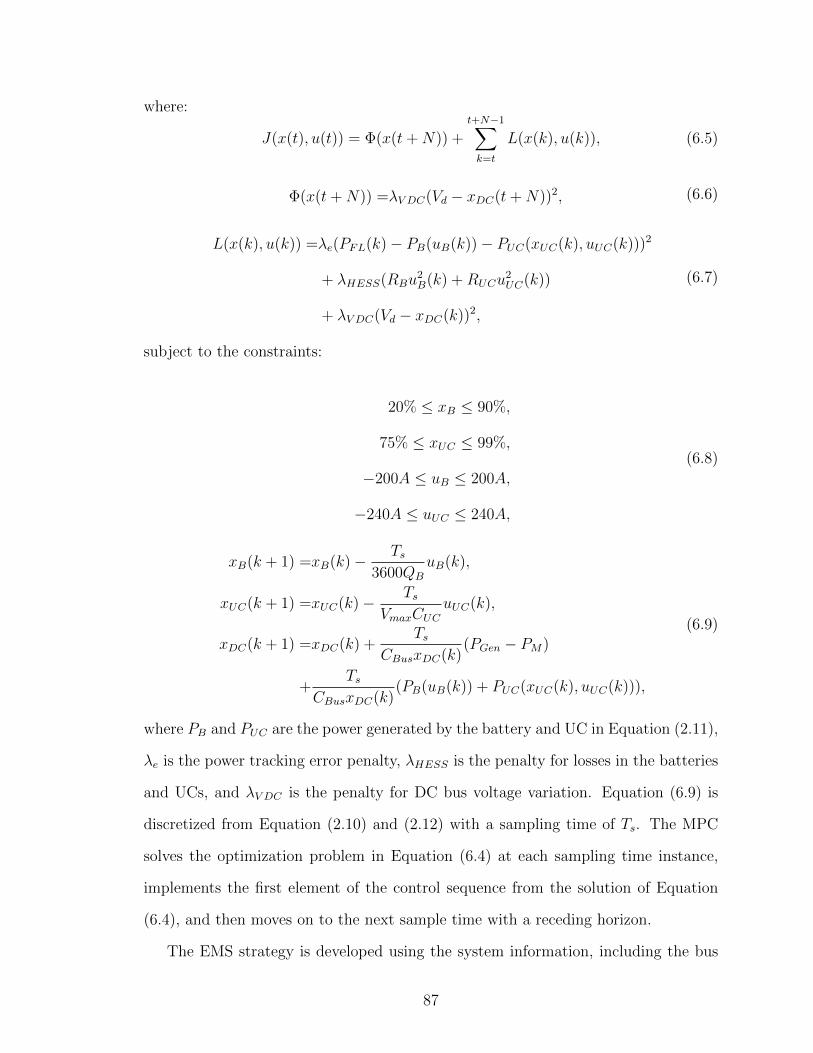
where:
J(x(t), u(t)) = Φ(x(t+N)) +t+N−1∑k=t
L(x(k), u(k)), (6.5)
Φ(x(t+N)) =λV DC(Vd − xDC(t+N))2, (6.6)
L(x(k), u(k)) =λe(PFL(k)− PB(uB(k))− PUC(xUC(k), uUC(k)))2
+ λHESS(RBu2B(k) +RUCu
2UC(k))
+ λV DC(Vd − xDC(k))2,
(6.7)
subject to the constraints:
20% ≤ xB ≤ 90%,
75% ≤ xUC ≤ 99%,
−200A ≤ uB ≤ 200A,
−240A ≤ uUC ≤ 240A,
(6.8)
xB(k + 1) =xB(k)− Ts3600QB
uB(k),
xUC(k + 1) =xUC(k)− TsVmaxCUC
uUC(k),
xDC(k + 1) =xDC(k) +Ts
CBusxDC(k)(PGen − PM)
+Ts
CBusxDC(k)(PB(uB(k)) + PUC(xUC(k), uUC(k))),
(6.9)
where PB and PUC are the power generated by the battery and UC in Equation (2.11),
λe is the power tracking error penalty, λHESS is the penalty for losses in the batteries
and UCs, and λV DC is the penalty for DC bus voltage variation. Equation (6.9) is
discretized from Equation (2.10) and (2.12) with a sampling time of Ts. The MPC
solves the optimization problem in Equation (6.4) at each sampling time instance,
implements the first element of the control sequence from the solution of Equation
(6.4), and then moves on to the next sample time with a receding horizon.
The EMS strategy is developed using the system information, including the bus
87

time [sec]475 480 485 490 495 500 505 510 515 520 525
[V]
4120
4140
4160
4180
4200
BL:Bus VoltageEMS:Bus Voltage
Frequency [Hz]0 2 4 6 8 10 12 14 16 18
[V]
0
2
4
6BL:Bus Voltage VariationEMS:Bus Voltage Variation
BL EMS
Figure 6.11: Performance comparison of BL and EMS: bus voltage response (topplots) and their frequency spectrums (bottom plots).
voltage, motor power, and ship propulsion load. This strategy is to minimize a cost
function that includes the power tracking error, DC bus voltage variation and HESS
electrical losses, subject to constraints of battery and ultra-capacitor SOC limits
and charging/discharging limits. As shown in Figure 6.11, the EMS more effectively
reduces the DC bus variation than the BL strategy does. Since the bus voltage error
is significantly reduced by the EMS, the generator will provide almost constant power,
which results in reduced fuel consumption.
6.1.5 Comparative Study and Simulation Results
To validate the interaction analysis and evaluate the different coordination strate-
gies, a comparative study is performed for the four strategies using the simulation-
oriented model. In order to quantify the performance of each strategy, the corre-
sponding performances have been evaluated in terms of the following metrics:
1. DC bus voltage variations measured by rms and maximum absolute value.
88

Table 6.2: Performance comparison of different control strategies.
Sea State 2.
BL MLF BVR EMSBus RMS Error 8.401V 11.76V 4.33V 2.16VBus Max Error 28.91V 39.15V 9.07V 6.10VPM/G RMS 23.18kW 27.65kW 8.01kW 4.14kWPM/G Max 72.77kW 103.59kW 27.36kW 10.01kWHESS Loss% N/A 0.34% 0.79% 0.24%IBhigh% N/A 0.0% 3.542% 0.0%
Sea State 4 (nominal condition).
BL MLF BVR EMSBus RMS Error 10.89V 11.75V 4.74V 2.47VBus Max Error 37.28V 40.51V 14.24V 3.24VPM/G RMS 31.75kW 27.14kW 10.83kW 4.69kWPM/G Max 97.22KW 104.67kW 38.64kW 13.12kWHESS Loss% N/A 0.44% 0.87% 0.29%IBhigh% N/A 0.146% 7.188% 0.0%
Sea State 6.
BL MLF BVR EMSBus RMS Error 24.87V 12.67V 9.70V 4.75VBus Max Error 52.32V 42.53V 21.28V 7.68VPM/G RMS 74.29kW 28.96kW 32.07kW 7.32kWPM/G Max 197.26kW 138.53kW 188.61kW 51.21kWHESS Loss% N/A 1.51% 1.70% 1.18%IBhigh% N/A 11.685% 38.771% 7.103%
2. Diesel-generator power fluctuations measured by rms and maximum absolute
value. The power fluctuations could cause additional fuel consumption and
mechanical wear and tear.
3. Efficiency in terms of power losses in the electrical system due to energy cycling.
4. Battery “friendliness” in terms of the time spent charging/discharging the bat-
tery at high currents. Numerous research results show that fast charging/discharging
can cause accelerated degradation in lithium battery systems [33]. We define
IBhigh% as the percentage of the high current operation (Ibattery ≥ 150A) over
the total operation time.
A quantitative comparison of different strategies is summarized in Table 6.2 at
three different sea states for a 24 second time frame. As can be seen, the results in
89

480 490 500 510 5204120
4140
4160
4180
4200
[V]
BL:Bus VoltageBVR:Bus Voltage
480 490 500 510 5204120
4140
4160
4180
4200
[V]
BL:Bus VoltageEMS:Bus Voltage
480 490 500 510 5203.25
3.3
3.35
3.4
3.45
3.5x 10
6
[W]
BL:PM/G PowerBVR:PM/G Power
480 490 500 510 5203.25
3.3
3.35
3.4
3.45
3.5x 10
6
[W]
BL:PM/G PowerEMS:PM/G Power
500 505 510 515 520 52584
85
86
87
88
89
90
[%]
BVR:UC SOCEMS:UC SOC
500 505 510 515 520 52579.98
79.99
80
80.01
80.02
80.03
80.04[%
]
BVR:Battery SOCEMS:Battery SOC
500 505 510 515 520 525−150
−100
−50
0
50
100
150
time [sec]
[A]
BVR:Battery Current
500 505 510 515 520 525−150
−100
−50
0
50
100
150
time [sec]
[A]
EMS:Battery Current
Figure 6.12: Performance comparison: BL, BVR and EMS.
Table 6.2 validate the interaction analysis discussed above. The performance from
best to worst are colored in the following sequence: blue, green, brown and red.The
MLF strategy achieves better performance at high sea states due to its effectiveness
in reducing the low frequency variation. However, at the nominal and low sea states,
90

Figure 6.13: Schematic of HESS-EMS for the electric propulsion system with HESS.
MLF performs much worse than the BL strategy because of its problems in the high
frequency range. The BVR strategy could better reduce some of the variations in the
DC bus voltage and generator power compared with the BL strategy. However, due to
the undesirable interaction with the generator, the BVR strategy incurs higher losses
and is less “friendly” to the battery, as shown in Table 6.2 and Figure 6.12. Compared
to the BVR case (see Figure 6.12), less SOC variations are observed for EMS. This
translates into an extended self-sustained operation time. To summarize, the EMS
achieves the best performance compared to other strategies in all the performance
metrics considered at all sea states.
6.2 Energy Management Strategies for the Integrated Con-
figuration
The EMS proposed in Section 6.1 incorporates information from the existing con-
trol system of the electric generation system and induction motor, and coordinates
the operation of the batteries and ultra-capacitors. While this strategy has the ad-
vantage of being “add-on” and “plug-in” in the sense that it requires no changes
to the existing control system of the generator sets and propulsion motor, it has no
91

authority to affect the generator and motor operation. This means that it is limited
in dealing with system interactions. Because of these limitations, large torque and
bus voltage variations have been observed in dynamic operation (such as pulse power
loads [41]-[43]), which force the HESS to operate at its limits.
This section proposes a new integrated EMS to encompass the controls of the
primary power sources and propulsion motor in addition to the HESS, to allow judi-
cious coordination that can achieve desired performance. The new integrated EMS
aims to increase system efficiency, enhance reliability, reduce mechanical wear and
tear, and improve load-following capability by eliminating unintended and adverse
interactions among the subsystems, especially in the dynamic load-following condi-
tions. The model-based analysis and simulation demonstrate the benefits, as well as
the potential cost, associated with the integrated EMS with system-level full-scale
coordination. The HESS EMS with HESS-level coordination presented in last section
is included to serve as a benchmark for the evaluation of the integrated EMS. This
benchmark is referred to as an HESS energy management strategy (HESS-EMS), be-
cause it is developed for HESS alone. The general diagram of the HESS-EMS system
is shown in Figure 6.13. While HESS-EMS can deal with some interactions among
subsystems, its effectiveness is limited because the actions it can take are limited by
the energy storage components. Compared to the benchmark, a comparison study
is performed using model predictive control to demonstrate the proposed integrated
EMS benefits.
6.2.1 Integrated System-Level EMS
To overcome the limitations of HESS-EMS in coordinating the power systems con-
nected to the shipboard micro-grid, The new EMS will integrate the generator sets,
electric motor, and HESS. It will be referred to as the system energy management
strategy (SYS-EMS), given that it breaks the boundaries of HESS and other subsys-
92

Figure 6.14: Schematic of SYS-EMS for the electric propulsion system with HESS.
tems. The general diagram of SYS-EMS is illustrated in Figure 6.14. In addition
to minimizing power tracking error, HESS energy loss, and bus voltage variation as
considered in HESS-EMS, the objectives of SYS-EMS include:
• keeping the motor shaft at its reference speed: min(ωd − xM);
• making the electric power generator and induction motor operate near their
most efficient operating points: min(P refGen − PGen) and min(P ref
M − PM);
• reducing the generator output variations: min(xG(k + 1)− xG(k));
• reducing mechanical wear and tear: min(uM(k)− uM(k − 1));
where ωd is the reference speed of the propulsion motor, and P refGen and P ref
M are the
reference powers of the generator sets and motor, respectively.
Therefore, the MPC formulation for SYS-EMS takes the following forms:
Φ(x(N)) =λV DC(Vd − xDC(N))2 + λω(ωd − xM(N))2, (6.10)
93

L(x(k), u(k)) =λV DC(Vd − xDC(k))2 + λω(ωd − xM(N))2
+ λPGen(P ref
Gen − xDC(k)xG(k))2
+ λPM(P ref
M − xM(k)uM(k))2
+ λ∆IPG(xG(k + 1)− xG(k))2
+ λ∆TM(uM(k)− uM(k − 1))2
+ λHESS(RBu2B(k) +RUCu
2UC(k)),
(6.11)
subject to the inequality constraints:
20% ≤ xB ≤ 90%,
75% ≤ xUC ≤ 99%,
0 ≤ xG ≤ 1000A,
0 ≤ xM ≤ 160RPM,
−200A ≤ uB ≤ 200A,
−240A ≤ uUC ≤ 240A,
−10V ≤ uG ≤ 10V,
−1.25× 10⁶Nm ≤ uM ≤ 1.25× 10⁶Nm,
(6.12)
94

and the equality constrains:
xB(k + 1) =xB(k)− Ts3600QB
uB(k),
xUC(k + 1) =xUC(k)− TsVmaxCUC
uUC(k),
xDC(k + 1) =xDC(k) +Ts
CBusxDC(k)(PB(uB(k)) + PUC(xUC(k), uUC(k))
+Ts
CBusxDC(k)(NGenxDC(k)xG(k)− xM(k)uM(k)/ηM),
xG(k + 1) =xG(k) +TsτPG
(−xG(k) +GPGuG(k)),
xM(k + 1) =xM(k) +TsH
(−βMxM(k) + uM(k)− TLoad(k)),
(6.13)
where λω, λPGenand λPM
are the penalties of tracking performance of motor speed,
generator power and motor power, respectively; λ∆IPGand λ∆TM
are the penalties
of the variations of generator output DC current and motor torque, respectively;
NGen = 2 is the number of generator sets, and ηM is the efficiency of the motor.
The main differences and the potential impact on performance and complexity
are discussed in the following remarks.
Remark 6.1: HESS-EMS is responsible for controlling the battery and UC charg-
ing/discharging, while SYS-EMS controls the entire electric propulsion system. HESS-
EMS has no authority to control the generator or propulsion motor. As shown in
Equations (6.10)-(6.11), comprehensive objectives, which consider the entire propul-
sion system performance, can be better formulated in SYS-EMS, leading to improved
performance over HESS-EMS. This will be shown in the next subsection, especially
when HESS is forced to operate at its limits.
Remark 6.2: Compared with SYS-EMS, HESS-EMS has the advantage of having
a “plug-in” capability. When a new HESS is introduced into the existing electric ship
propulsion system, HESS-EMS requires no change the existing control systems of the
generator sets and propulsion motor. A further advantage of HESS-EMS is that it
95

has a lower computational cost than SYS-EMS.
6.2.2 Comparative Study and Simulation Results
To evaluate the proposed SYS-EMS and quantify the performance advantages
introduced by system-level coordination, a comparative study is performed and the
following key metrics are used for both HESS-EMS and SYS-EMS:
1. DC bus voltage variations measured by rms and maximum absolute value;
2. Motor speed variations measured by rms and maximum absolute value.
3. High frequency variations of propulsion motor torque measured by the maxi-
mum amplitude of the torque frequency spectrums in the high-frequency range
(i.e., greater than 1Hz);
4. Efficiency in terms of power losses of HESS in the electrical system due to energy
cycling;
5. Battery “friendliness” in terms of the time spent charging/discharging the bat-
tery with high currents.
As shown in Figure 6.15, both the HESS-EMS and SYS-EMS offer good regula-
tion of the DC bus voltage. However, the SYS-EMS significantly reduces the torque
variation with almost the same performance in motor speed tracking compared to
HESS-EMS. Due to the multi-frequency characteristics of the load fluctuations, there
is a trade-off among speed variation, torque variation, and power variation. Desired
performance can be achieved in SYS-EMS by tuning the penalties in the cost function.
When a large pulse load is applied, the coordination of the generator sets, propulsion
motor, and HESS is able to address the dynamic operating conditions. As shown in
Figure 6.16, when a 500KW pulse load of 1 second duration and 6 second period is
applied, SYS-EMS uses all the subsystems, including the generator and propulsion
96
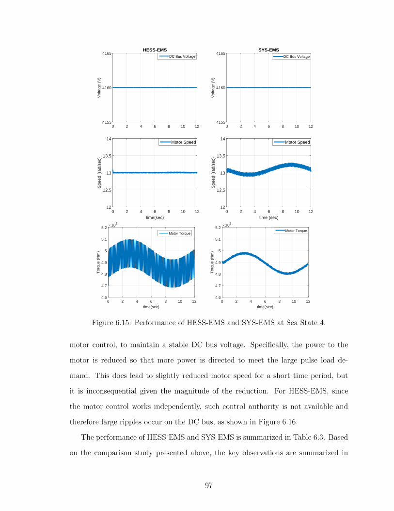
0 2 4 6 8 10 12
Vol
tage
(V
)
4155
4160
4165HESS-EMS
DC Bus Voltage
0 2 4 6 8 10 12
Vol
tage
(V
)
4155
4160
4165SYS-EMS
DC Bus Voltage
time(sec)0 2 4 6 8 10 12
Spe
ed (
rad/
sec)
12
12.5
13
13.5
14Motor Speed
time (sec)0 2 4 6 8 10 12
Spe
ed (
rad/
sec)
12
12.5
13
13.5
14Motor Speed
time(sec)0 2 4 6 8 10 12
Tor
que
(Nm
)
×105
4.6
4.7
4.8
4.9
5
5.1
5.2Motor Torque
time(sec)0 2 4 6 8 10 12
Tor
que
(Nm
)
×105
4.6
4.7
4.8
4.9
5
5.1
5.2Motor Torque
Figure 6.15: Performance of HESS-EMS and SYS-EMS at Sea State 4.
motor control, to maintain a stable DC bus voltage. Specifically, the power to the
motor is reduced so that more power is directed to meet the large pulse load de-
mand. This does lead to slightly reduced motor speed for a short time period, but
it is inconsequential given the magnitude of the reduction. For HESS-EMS, since
the motor control works independently, such control authority is not available and
therefore large ripples occur on the DC bus, as shown in Figure 6.16.
The performance of HESS-EMS and SYS-EMS is summarized in Table 6.3. Based
on the comparison study presented above, the key observations are summarized in
97
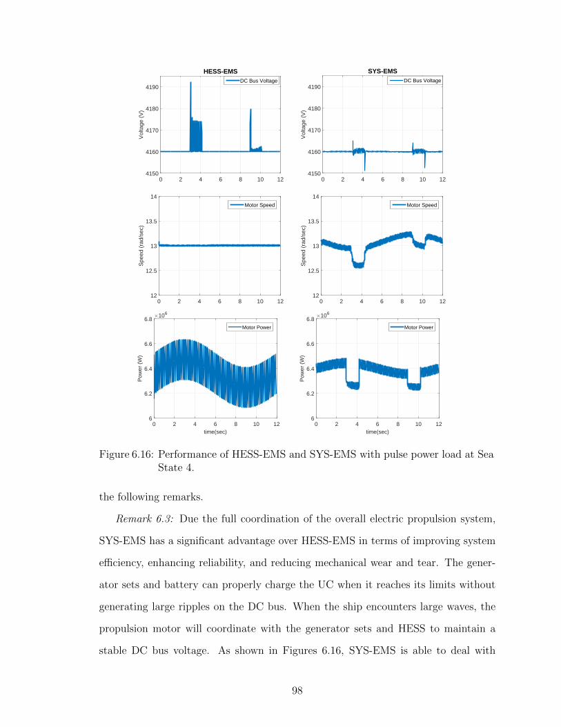
0 2 4 6 8 10 12
Vol
tage
(V
)
4150
4160
4170
4180
4190
HESS-EMSDC Bus Voltage
0 2 4 6 8 10 12
Vol
tage
(V
)
4150
4160
4170
4180
4190
SYS-EMSDC Bus Voltage
0 2 4 6 8 10 12
Spe
ed (
rad/
sec)
12
12.5
13
13.5
14Motor Speed
0 2 4 6 8 10 12S
peed
(ra
d/se
c)12
12.5
13
13.5
14Motor Speed
time(sec)0 2 4 6 8 10 12
Pow
er (
W)
×106
6
6.2
6.4
6.6
6.8Motor Power
time(sec)0 2 4 6 8 10 12
Pow
er (
W)
×106
6
6.2
6.4
6.6
6.8Motor Power
Figure 6.16: Performance of HESS-EMS and SYS-EMS with pulse power load at SeaState 4.
the following remarks.
Remark 6.3: Due the full coordination of the overall electric propulsion system,
SYS-EMS has a significant advantage over HESS-EMS in terms of improving system
efficiency, enhancing reliability, and reducing mechanical wear and tear. The gener-
ator sets and battery can properly charge the UC when it reaches its limits without
generating large ripples on the DC bus. When the ship encounters large waves, the
propulsion motor will coordinate with the generator sets and HESS to maintain a
stable DC bus voltage. As shown in Figures 6.16, SYS-EMS is able to deal with
98

the load fluctuations and pulse power load simultaneously and achieve the desired
performance.
Remark 6.4: The disadvantage of SYS-EMS compared to HESS-EMS is the high
computational cost. Therefore, to implement SYS-EMS in real-time control applica-
tions, computationally-efficient optimization algorithms are needed.
The proposed two EMSs, namely HESS-EMS and SYS-EMS, effectively mitigate
the propulsion load effect on the shipboard network, in terms of enhanced reliability,
improved efficiency, reduced mechanical wear and tear. The study in this chapter
assumes the propulsion load torque is known. However, in most marine applications,
the propulsion load torque is immeasurable and unpredictable. In order to address
this issue, the load torque estimation and prediction are studied in the next chapter.
6.3 Summary
In this chapter, two configurations are studied to integrate the new HESS with
an existing propulsion system: a ‘plug-in’ configuration and an ‘integrated’ config-
uration. The trade-off between control simplicity, modularity and overall system
performance is discussed. The ‘plug-in’ configuration provides a simple and modular
control solution. The interaction of different control strategies for ‘plug-in’ configu-
ration is analyzed. For the ‘integrated’ configuration, the integrated approach takes
advantage of the predictive nature of MPC and allows the designers to judiciously
coordinate the different entities of the shipboard network under constraints, thereby
providing benefits to system performance. This ‘integrated’ strategy requires the
information of propulsion-load torque, which will be studied in the next chapter.
99

Table 6.3: EMS performance comparison.
Sea State 4.Operation time:1200 sec; without pulse power load
HESS-EMS SYS-EMSBus Voltage RMS Error 0.9148V 0.0005VBus Voltage Max Error 61.0588V 0.0015VMotor Speed RMS Error 0.0851rad/sec 0.11rad/secMotor Speed Max Error 0.1004rad/sec 0.2017rad/secMotor Torque Variation 11.747KNm 0.799KNmHESS Loss% 1.496% 0.3754%IBhigh% 0.7133% 0.0%
Sea State 6.Operation time:1200 sec; without pulse power load
HESS-EMS SYS-EMSBus Voltage RMS Error 20.6632V 0.001VBus Voltage Max Error 159.1228V 0.0023VMotor Speed RMS Error 0.0849rad/sec 0.3923rad/secMotor Speed Max Error 0.1036rad/sec 1.0686rad/secMotor Torque Variation 24.903KNm 0.83KNmHESS Loss% 2.3391% 1.157%IBhigh% 5.7767% 0.0%
Sea State 4.Operation time:12 sec; with 500KW pulse power load
HESS-EMS SYS-EMSBus Voltage RMS Error 3.1259V 0.7016VBus Voltage Max Error 32.3337V 8.83841VMotor Speed RMS Error 0.0851rad/sec 0.2206rad/secMotor Speed Max Error 0.1004rad/sec 0.6536rad/secMotor Torque Variation 12.88KNm 0.96KNmHESS Loss% 1.7602% 1.7543%IBhigh% 4.8333% 0.1667%
Sea State 6.Operation time:12 sec; with 500KW pulse power load
HESS-EMS SYS-EMSBus Voltage RMS Error 3.1296V 0.6182VBus Voltage Max Error 28.169V 9.8445VMotor Speed RMS Error 0.0849rad/sec 0.4301rad/secMotor Speed Max Error 0.1036rad/sec 0.8820rad/secMotor Torque Variation 12.86KNm 0.879KNmHESS Loss% 2.3391% 1.3573%IBhigh% 5.7767% 0.1667%
100

CHAPTER VII
Load Torque Estimation and Prediction for An
Electric Ship Propulsion System
In previous chapters, we have developed an integrated EMS using MPC to address
the effects of the load fluctuations and achieve the desired performance. However, it is
assumed that the propulsion-load torque is known and can be accurately predicted. In
most marine applications, however, the propulsion-load torque is difficult to measure
and includes multi-frequency fluctuations. Given the importance of the propulsion-
load torque, this chapter focuses on its estimation and prediction for implementing
MPC.
Load-torque estimation has been explored in a number of studies [19, 21, 22, 83,
84, 85]. In [19, 21, 22, 83], the load torque is assumed to be constant or slowly
time-varying. For our problem, the load torque investigated here consists of multi-
frequency fluctuation components. The disturbance observer or input observer (IO)
approach presented in [84, 85], on the other hand, is not based on the assumption that
the load torque is constant or slowly time-varying. Note that the input observer is
also referred to as the disturbance observer in the literature, since the unknown input
can be considered as a disturbance [86]. Despite the contributions of these works,
the aforementioned approaches do not take advantage of the physical characteristics
of the propulsion-load dynamics, especially the fast dynamics. Furthermore, those
101

approaches cannot be directly used to predict the future load torque, which is required
for implementing MPC. Additional load predictive capabilities are therefore required.
In this chapter, we develop a model-based approach to estimate the propulsion-
load torque for all-electric ships. Due to the complexity of the propulsion-load torque
model, we first develop a simplified model which is able to capture the key dynam-
ics. Because of uncertainties in the model parameters, parameter identification is
used, leading to improved robustness of the control system. This model-based ap-
proach can be easily integrated with the MPC to formulate an adaptive load esti-
mation/prediction with MPC (AMPC). In order to evaluate the proposed AMPC
approach, the IO presented in [85] is used as an alternative technique to estimate
the propeller-load torque. In this alternative control, linear prediction (LP) [87] is
combined with IO to predict the future propulsion-load torque. A comparative study
is performed to evaluate the effectiveness of the proposed AMPC in terms of mini-
mizing the bus voltage variation, regulating the rotational speed, and reducing the
high-frequency motor torque variation. The implications of accurate estimation and
prediction are also illustrated and analyzed in this study.
Table 7.1: Control objectives and their mathematical expression.Control objectives Mathematical expressionSystem reliability min(Vd − xDC(k))2
Thrust production min(ωd − xM (k))2
System efficiencymin(P ref
Gen − xDC(k)xG(k))2
min(P refM − xM (k)uM (k))2
min(RBu2B(k) + RUCu
2UC(k))
Wear-and-tear mitigationmin(xG(k + 1)− xG(k))2
min(uM (k)− uM (k − 1))2
min(xM (k + 1)− xM (k))2
102

7.1 Energy Management Strategy Formulation
7.1.1 AMPC Problem Formulation
In order to achieve enhanced system reliability, desired thrust production, im-
proved system efficiency, and reduced wear and tear, the corresponding control ob-
jectives and their mathematical expressions are summarized in Table 7.1, where Vd is
the desired bus voltage, ωd is the desired reference speed of the propulsion motor, and
P refGen and P ref
M are the reference powers of the generator sets and motor, respectively.
Since the propulsion-load torque TLoad in (2.14) is difficult to measure for ma-
rine applications, estimation of TLoad is required. Furthermore, in order to implement
MPC, prediction of TLoad in the MPC prediction windows is also required. To address
the estimation and prediction of the propulsion-load torque, an adaptive load estima-
tion/prediction with MPC is developed which minimizes a cost function subject to
constraints within the prediction horizon. This can be mathematically expressed as
follows:
P (x0) : minx:[t,t+N ]→R5u:[t,t+N−1]→R4
J(x, u, TLoad) (7.1)
where:
J(x, u, TLoad) = Φ(x(t+N)) +t+N−1∑k=t
L(x(k), u(k), TLoad(k|t)), (7.2)
subject to:
x(k + 1) = f(x(k), u(k), TLoad(k|t)), x(t) = x0, (7.3)
C(x(k), u(k)) ≤ 0, (7.4)
where Φ(x(N)) and L(x(k), u(k), TLoad(k|t)) are the terminal and instantaneous cost
functions, N is the time window over which the cost will be evaluated, C(x(k), u(k))
103

represents the inequality constraints, t represents the current time, and x(k), u(k)
are the instantaneous values of the states and inputs at time k, respectively. The
instantaneous estimation of the propulsion-load torque is represented by TLoad(t|t),
and TLoad(k|t) for k = t + 1, ..., t + N − 1 are the predictions of the load torque at
time t.
According to the control objectives as shown in Table 7.1, the AMPC formulation
takes the following form:
Φ(x(N)) =λV DC(Vd − xDC(N))2 + λω(ωd − xM(N))2, (7.5)
L(x(k), u(k), TLoad(k|t)) =λV DC(Vd − xDC(k))2
+ λω(ωd − xM(k))2
+ λPGen(P ref
Gen − xDC(k)xG(k))2
+ λPM(P ref
M − xM(k)uM(k))2
+ λHESS(RBu2B(k) +RUCu
2UC(k))
+ λ∆IPG(xG(k + 1)− xG(k))2
+ λ∆TM(uM(k)− uM(k − 1))2
+ λ∆ω(xM(k + 1)− xM(k))2,
(7.6)
for all k ∈ [t, t + N − 1], subject to (6.12) and (6.13), where λV DC , λω, λPGen, λPM
,
λHESS, λ∆IPG, λ∆TM
and λ∆ω are the weighting factors for the penalties of DC bus
voltage variation, tracking performance of motor speed, generator and motor power,
HESS losses, variations of generator output DC current, motor torque and motor
speed, respectively. The estimation and prediction of propulsion load torque is ad-
dressed in the following section.
104

7.2 Propulsion-load Torque Estimation and Prediction
7.2.1 First Approach: Input Observer with Linear Prediction
In order to estimate the propulsion load torque, the input observer (IO) presented
in [85] is used. The general propeller-motor dynamic is described by the following
equation:
ω =TM(t)− βMω − TLoad(t)
H. (7.7)
We define
uL(t) = TLoad(t)/H,
zL(t) =TM(t)− βMω(t)
H,
yL(t) = ω(t) + ξL(t),
(7.8)
where ξL(t) is the measurement noise.
The unknown input uL(t) can be then estimated by the following equations [85]:
uL(t) = εL(t) + αLy(t) + φL(t),
φL = −αLφl − αLzL,
εL = −αLεL − α2LyL,
TLoad(t) = uL(t)H,
(7.9)
where αL > 0 is the observer gain and the states of the observer are φL and εL.
Since the input observer cannot predict future load torque, linear prediction is
used. Linear prediction incorporates the knowledge of the signal frequency spectrum
(autocorrelation) to determine the linear prediction coefficients (LPCs). Only past
data, which can be obtained from IO estimation results, is required for LP. To predict
the load torque at time t+1, linear prediction is formulated as follows:
105

TLoad(t+ 1|t) =
NLP∑i=1
βLPiTLoad(t− i+ 1|t), (7.10)
where NLP is the prediction order, and βLPi(i = 1, ..., NLP ) are the linear prediction
coefficients. The coefficients can be calculated using the Matlab function “lpc”. The
inputs of “lpc” are the past data and the desired prediction order. We then com-
bine IO with LP. The algorithm can be easily implemented, as shown in Figure 7.2.
However, there are several limitations of this approach, summarized in the following.
Remark 7.1: The gain αL in (7.9) is the only parameter used to tune IO. Since
the high-frequency fluctuation is at the propeller-blade frequency, i.e., around 8Hz,
the minimum cut-off frequency is designed at 8Hz, leading to a minimum observer
gain αL = 50. As shown in Figure 7.1, the phase shift at the cut-off frequency is
about 45 degrees, which might significantly affect the estimation performance. In
order to reduce the estimation error, the high-gain input observer is a reasonable
choice if the noise can be ignored. However, noise is an issue under many conditions;
the estimation performance of a high-gain observer, e.g. αL = 400, might be even
worse than one using the minimum gain. The maximum observer gain is difficult to
determine when the noise is random and unknown.
Remark 7.2: The predictive performance of LP highly depends on past data. The
performance of IO directly affects LP. Furthermore, the predictive error could be
accumulated as the predictive horizon extends. For example, predicting TLoad(t +
2|t) requires the prediction value TLoad(t + 1|t), which means the predictive error of
TLoad(t+ 1|t) affects the prediction of TLoad(t+ 2|t).
Since only the general propeller-motor model (7.7) is used in this approach, the
dynamics of the propeller load torque are not taken into consideration. In order to
address the limitations discussed in Remarks 7.1 and 7.2, a model-based approach
is required, leading to the adaptive load estimation/prediction with model predictive
control discussed in the next section. The major challenge of this approach is the
106

Mag
nitu
de (
dB)
-50
-40
-30
-20
-10
0
10-1 100 101 102 103
Pha
se (
deg)
-135
-90
-45
0
Continuous System: Bode Plot
Discrete System: Bode Plot
Bode Diagram
Frequency (Hz)
System: Discrete System: Bode PlotFrequency (Hz): 7.58Phase (deg): -43.7
Figure 7.1: Bode plot of the input observer.
Figure 7.2: Schematic diagram of the first approach (IO-LP).
complexity of the load torque model (7.11). The focus of the next section is to
develop a simplified model of (7.11), which is able to capture the key dynamics of the
propeller-load torque.
7.2.2 Second Approach: Adaptive Load Estimation/Prediction with Model
Predictive Control
Instead of using only the general propeller-motor model (7.7), this model can
be augmented by the propeller-load torque model presented in Chapter II to provide
additional useful information to estimate the load torque. This propulsion-load torque
107

model is expressed in the following:
TLoad(t) = sgn(n)βρn2D5fKQ(JA, P itch/D,Ae/Ao, Z,Rn)
= sgn(n)βρD5
(c0n
2 + c1U(1− w)
Dn
)+ sgn(n)βρD5c2
(U(1− w)
D
)2
+ sgn(n)βρD5c3
(U(1− w)
D
)31
n,
(7.11)
where,
n = ω/2π,
1− w = M0 −M1cos(4θ),
θ is the angular position of one blade; ci (i=0,1,2,3), M0 and M1 are unknown param-
eters; β is the loss factor; ρ is the density of water; D is the diameter of the propeller;
and fKQis the torque coefficient function. In fKQ
, JA is the advance coefficient;
Pitch/D is the pitch ratio; Ae/Ao is the expanded blade-area ratio, with Ae being
the expanded blade area and Ao being the swept area; Z is the number of propeller
blades; and Rn is the Reynolds number.
The parameters in (7.11) are usually fitted off-line. For example, parameters c0,1,2,3
in the function fKQare based on the fitted KQ curves for the Wageningen B-Series
Propellers [70] and the KQ correction multiplier [71]. The multiplier in [71] is chosen
to minimize the error in the range of the maximum efficiency. If the propeller is not
operating in the range of maximum efficiency, the error could be significantly larger.
Furthermore, the coefficients in fKQcan vary with the wear and tear of the propeller.
As the operating environment changes, the parameters in the propeller-load model
(7.11) can also change. Therefore, to use (7.11) for load torque estimation, online
parameter identification is necessary.
In this detailed load model (7.11), six parameters (c0, c1, c2, c3,M0,M1) are used in
the nonlinear parametric model, making parameter estimation difficult. To facilitate
108

315 320 325
Tor
que
(Nm
)
×105
5
5.2
5.4
SS4
Detailed ModelSimplified Model 319 319.2 319.4 319.6 319.8 320
×105
5
5.2
5.4
5.6SS4 (Zoom in)
time (sec)315 320 325
Tor
que
(Nm
)
×105
4.8
5
5.2
5.4
SS6
time (sec)319 319.2 319.4 319.6 319.8 320
×105
5
5.2
5.4
5.6SS6 (Zoom in)
Figure 7.3: Outputs of the detailed and simplified propeller-load torque models atsea state 4 (top) and sea state 6 (bottom).
online parameter estimation, we propose the following simplified model (7.12), whose
derivation is given in the Appendix (Section 7.5).
TLoad ≈ C1 + C2cos(4θ) + C3(n− nref ). (7.12)
The output of the detailed propeller-load torque model and the simplified model
(7.12) at sea states 4 and 6 are shown in Figure 7.3.
With the combination of (7.7) and (7.12), the new propeller-motor model is de-
veloped in the following:
ω =TM(t)− βMω − (C1 + C2cos(4θ) + C3∆ω/2π)
H. (7.13)
For parameter estimation, a parametric model is defined as follows:
zpar = C∗Tparφpar, (7.14)
109

where
zpar =
λpar
s+ λpar
(ω − 1
H(TM − βMω)
),
C∗par =[C1 C2 C3]T ,
φpar =
−λpars+ λpar
[1 cos(4θ) ∆ω/2π]T ,
λpar is the filter gain, and · represents the dynamic operator of the filter, whose
transfer function is (·). The filter is introduced to avoid taking numerical derivatives
in estimation.
The normalized gradient algorithm is chosen as the adaptive law and presented in
the following [88]:
Cpar(t) = Cpar(t− 1)+TsΓφpar(t)εpar
1 + φpar(t)Tφpar(t),
where
εpar = zpar(t)− Cpar(t− 1)Tφpar(t),
and Γ = ΓT is a positive-definite matrix satisfying the criteria that the real part of
its eigen-values are between (0, 2/Ts), which affects how fast Cpar updates.
The speed variation within the predictive horizon is assumed to be very small,
i.e., xM(t + N − 1) ≈ xM(t + N − 2) ≈ ... ≈ xM(t). This results in an estimation of
the future propeller-blade position at time k as follows:
θ(k) = θ(t) + (k − t)Tsx2(t). (t ≤ k ≤ t+N − 1)
Therefore, the schematic diagram of the proposed AMPC is shown in Figure 7.4, and
the new propeller-motor dynamic is expressed in the following:
110

Figure 7.4: Schematic diagram of the AMPC controller.
Table 7.2: Performance metrics.
Performance Mathematical expression
“Voltage Regulation”
√∑NTk=0(Vd−xDC(k))2
NT +1
“Speed Regulation”
√∑NTk=0(ωd−xM (k))2
NT +1
“Gen Power Tracking”
√∑NTk=0(P ref
Gen−xDC(k)xG(k))2
NT +1
“Motor Power Tracking”
√∑NTk=0(P ref
M −xM (k)uM (k))2
NT +1
“HESS Losses Reduction”
√∑NTk=0(RBu2
B(k)+RUCu2UC(k))
NT +1
“Gen Oscillation Reduction”
√∑NTk=0(xG(k+1)−xG(k))2
NT +1
“Torque Oscillation Reduction”
√∑NTk=0(uM (k)−uM (k−1))2
NT +1
“Speed Oscillation Reduction”
√∑NTk=0(xM (k+1)−xM (k))2
NT +1
“Total Cost”
√∑NTk=0 L(x(k),u(k),TLoad(k))
NT +1
xM(k + 1) =xM(k)− TsC3
2πH(xM(k)− ωd)
+TsH
(uM(k)− βMxM(k)− C1)
− TsHC2cos(4(θ(t) + (k − t)TsxM(t))),
(7.15)
for all k ∈ [t, t+N − 1].
111

7.3 Performance Evaluation and Discussion
According to the control objectives, the performance metrics are presented in
Table 7.2, where NT equals [(tT − t0)/Ts], with [·] representing integer rounding, t0
and tT are the initial and final values of the time period being investigated, and
L(x(k), u(k), TLoad(k)) represents the cost function in Equation (7.6). In order to
evaluate the proposed approaches to load torque estimation and prediction, the results
obtained by six cases have been studied and analyzed in this section. These six cases
are described in the following:
• Case 1 “Ideal”: In this case, the detailed propulsion-load torque model (7.11)
without any uncertainty is used to obtain the load torque. Nonlinear MPC uses
the perfect model to predict the future load torque in its optimization. Because
there is no uncertainty in this case, it is referred to as “Ideal”.
• Case 2 “Frozen prediction”: In this case, the instantaneous load torque is ob-
tained from the load torque model (7.11) without any uncertainty. Compared
to Case 1, the future load torque used in the MPC is assumed to be same as
the instantaneous load torque, i.e., TLoad(t + N − 1|t) = TLoad(t + N − 2|t) =
... = TLoad(t|t), so called “Frozen prediction”.
• Case 3 “LP-Only”: Different from Case 2, the future load torque in this case
is predicted using LP. The true load torque is used as the instantaneous load
torque.
• Case 4 “IO-Frozen prediction”: In this case, the input observer is used, instead
of the true load torque. The future load torque is assumed to be the same as
the IO estimation.
• Case 5 “IO-LP”: The first approach, i.e., IO combined with LP, is used in this
case.
112

SS4 SS6
Tor
que
Err
or (
kNm
)
0
5
10
15
Estimation ErrorInput Observer (Case 4)Input Observer (Case 5)Adaptive Load Estimation (Case 6)
Figure 7.5: Estimation error of the adaptive load estimation and input observer.
• Case 6 “AMPC”: This case is the proposed AMPC.
We first evaluate the estimation performance. Among these six cases, Cases 4, 5,
and 6 require estimation of the load torque. As shown in Figure 7.5, adaptive load
estimation has better estimation performance than the input observer. The reason
is that more propeller-load information is taken into consideration in this adaptive
approach.
The key performance metrics and results are presented in Table 7.3. The perfor-
mance results of each case are normalized by Case 1. The smaller value represents
the better performance. Note that the performance of Cases 2-6 from best to worst
are colored in the following sequence: blue, green, yellow, brown and red. The
degraded performance (%) is defined as the performance of Case 2 5 in Table 7.3
minus 1 (as all of the performance are normalized by Case 1), and then times 100%.
As can be seen in Table 7.3, the performance of Case 6 is the closest to Case 1.
Case 1 uses the accurate detailed propeller-load model and takes its dynamics into
consideration, leading to the best performance among all of the investigated cases.
The “Total Cost” in the performance metrics represents the overall performance,
113

Table 7.3: Performance comparison.
Sea State 4.Performance Metrics Case 1 Case 2 Case 3 Case 4 Case 5 Case 6“Voltage Regulation” 1 27.77 27.76 28.15 28.07 1.036“Speed Regulation” 1 1.043 1.043 1.057 1.057 0.995
“Gen Power Tracking” 1 1.095 1.057 1.251 1.179 1.148“Motor Power Tracking” 1 1.116 1.162 1.154 1.185 1.151
“HESS Losses Reduction” 1 1.185 1.189 1.247 1.227 1.184“Gen Oscillation Reduction” 1 1.055 1.011 1.384 1.286 0.985
“Torque Oscillation Reduction” 1 2.803 1.792 3.067 2.609 2.172“Speed Oscillation Reduction” 1 1.186 1.178 1.198 1.194 1.025
“Total Cost” 1 1.412 1.335 1.456 1.414 1.106
Sea State 6.“Bus Regulation” 1 24.63 24.61 24.97 24.97 1.328
“Speed Regulation” 1 1.032 1.029 1.045 1.045 1.027“Gen Power Tracking” 1 1.267 1.254 1.438 1.318 1.241
“Motor Power Tracking” 1 1.147 1.144 1.163 1.151 1.099“HESS Losses Reduction” 1 1.166 1.174 1.189 1.197 1.194
“Gen Oscillation Reduction” 1 1.307 1.578 2.167 1.649 1.128“Torque Oscillation Reduction” 1 2.206 1.590 2.376 2.178 1.230“Speed Oscillation Reduction” 1 1.216 1.196 1.246 1.242 1.052
“Total Cost” 1 1.123 1.085 1.149 1.130 1.009
which takes all of the other metrics along with their priorities (i.e., their weighting
factors) into consideration. According to “Total Cost”, the performance from the
best to the worst are Case 1 (“Ideal”), Case 6 (“AMPC”), Case 3 (“LP-Only”), Case
2 (“Frozen prediction”), Case 5 (“IO-LP”), and Case 4 (“IO-Frozen prediction”) at
both sea states 4 and 6. Based on the performance comparison, the key observations
are presented in the following Remarks.
Remark 7.3 (Effects of load prediction): Cases 1, 2 and 3 all assume perfect load
estimation at time t, but use different load predictions. Case 1 takes the load dynam-
ics into consideration, and Case 3 uses the signal spectrum (correlation) information
to predict future torque, while Case 2 uses none of these, leading to the worst per-
formance of the three cases. The “Total Cost” performance degradation of Cases 2
and 3 compared to Case 1 is shown in Figure 7.6. Another comparative result can be
shown between Cases 4 and 5. Both Cases 4 and 5 use the input observer to estimate
Tload(t|t), but differ in the prediction scheme. The “Total Cost” degradation of Cases
4 and 5 compared to Case 1 is shown Figure 7.7. Note that the difference between
114

SS4 SS6
Deg
rade
d P
erfo
rman
ce (
%)
0
10
20
30
40
50Total Cost
Case 2Case 3
Figure 7.6: Cases 2 and 3 degraded “Total Cost” performance compared to Case 1.
SS4 SS6
Deg
rade
d P
erfo
rman
ce (
%)
0
10
20
30
40
50Total Cost
Case 4Case 5
Figure 7.7: Cases 4 and 5 degraded “Total Cost” performance compared to Case 1.
Cases 4 and 5 is smaller than that between Cases 2 and 3, because the estimation
error in Case 5 influences the prediction performance.
Remark 7.4 (Effects of load estimation): The difference between Case 2 and Case
4 is in the load torque estimation, where the former uses the accurate load torque
model but the latter employs an IO to estimate the load torque. Case 2 outperforms
Case 4 in most of the performance metrics. Their “Total Cost” performance is shown
115

SS4 SS6
Deg
rade
d P
erfo
rman
ce (
%)
0
10
20
30
40
50Total Cost
Case 2Case 4
Figure 7.8: Cases 2 and 4 degraded “Total Cost” performance compared to Case 1.
in Figure 7.8. Similarly, Case 3 and Case 5 use the same prediction method, but have
different load estimation. As shown in Figure 7.9, the difference between Cases 3 and
5 is larger than that between Cases 2 and 4. This is because the estimation affects
not only the instantaneous information, but also the prediction in Cases 3 and 5.
Case 1 has better performance than Case 6 as expected, due to the uncertainties in
the dynamic model used for AMPC. These comparisons demonstrate that load torque
estimation plays a key role in achieving good performance.
Remark 7.5 (Effects of data-based LP): Except for Cases 1 and 6, Case 3 has the
best performance among the remaining 4 cases. Even though Case 3 only has the
data-based load predictor, the prediction still contributes some benefits, especially
with regard to reducing wear and tear. As shown in Figure 7.10, the metric “Torque
Oscillation Reduction” demonstrates that Case 3 can achieve almost the same small
motor torque variations as Case 6. Moreover, Case 3 outperforms Cases 2, 4 and 5 in
terms of metrics “Gen Oscillation Reduction” and “Speed Oscillation Reduction”, as
shown in Table 7.3, further demonstrating the benefits of LP in performance metrics
of reducing the wear and tear of the motor and generator sets. Compared to Case 3,
116
SS4 SS6
Deg
rade
d P
erfo
rman
ce (
%)
0
10
20
30
40
50Total Cost
Case 3Case 5
Figure 7.9: Cases 3 and 5 degraded “Total Cost” performance compared to Case 1.
Case 5 also uses LP to predict future torque. However, the estimation error of the
input observer affects the prediction performance, as discussed in Remark 7.2. As
can be seen, at sea state 4, Case 5 can achieve performance similar to Case 2. At sea
state 6, the performance of Case 5 is worse than Case 2. This comparison illustrates
that the load torque estimation is essential to improve the performance of data-based
LP.
Remark 7.6 (Effects of adaptation): Case 6 is the only case that achieves compet-
itive performance to Case 1. This is because only these two cases truly capture the
load dynamics by using the propulsion-load torque model, thereby maintaining the
motor and generator sets working around the reference points through coordination of
subsystems. Without the ability to capture the load torque dynamics, however, other
cases need the assistance of the motor and generator sets to mitigate the bus voltage
variations, leading to degraded system efficiency and increased wear and tear. In
order to evaluate the effects of adaptation, a comparative study is performed between
Case 6 and Case 1 with 2% modeling errors (2%Err), where 2% modeling errors are
added on c0 and M0 (which have the most significant effects in the propulsion-load
117

SS4 SS6
Deg
rade
d P
erfo
rman
ce (
%)
0
50
100
150
200
250Torque Oscillation Reduction
Case 2Case 3Case 4Case 5Case 6
Figure 7.10: Cases 2-6 degraded “Torque Oscillation Reduction” performance com-pared to Case 1.
torque model). As shown in Table 7.4, these 2% modeling errors (without adapta-
tion) can cause “Total Cost” 100% and 40% higher than Case 6 (with adaptation)
at sea state 4 and 6, respectively. Moreover, the performance of 2%Err is even much
worse than Case 5 (IO-Only). The key factors that renders favorable performance of
AMPC are summarized in the following:
• The foundation of AMPC is a well-developed simplified model that captures the
essential dynamics of the load torque. With accurate parameter identification,
AMPC can predict the future load torque much better than LP.
• When the load torque dynamic model is integrated into the MPC controller,
AMPC truly takes the load torque dynamic into consideration, resulting in the
unique advantage of AMPC compared to the other 4 cases (Case 2, 3, 4 and 5).
Remark 7.7 (Effects of weighting factors): The weighting factors can undoubtedly
influence the performance of the proposed AMPC. Each weighting factor λ assigns
a relative priority to a performance aspect. As the main objectives, the system
reliability and thrust production have the highest priority. The weighting factor can
be tuned with emphasis being placed on different performance attributes, such as
118

Table 7.4: Performance comparison: Case 6 vs. Case 1 with 2% modeling error.
Performance MetricsSS4 SS6
Case 6 2% ERR Case 6 2% ERR“Voltage Regulation” 1.036 11.26 1.328 9.125“Speed Regulation” 0.995 2.074 1.027 1.585
“Gen Power Tracking” 1.148 3.226 1.241 1.827“Motor Power Tracking” 1.151 1.598 1.099 7.829
“HESS Losses Reduction” 1.184 3.438 1.194 1.502“Gen Oscillation Reduction” 0.985 4.038 1.128 2.885
“Torque Oscillation Reduction” 2.172 1.467 1.230 1.155“Speed Oscillation Reduction” 1.006 1.014 1.052 1.02
“Total Cost” 1.106 2.190 1.009 1.410
Table 7.5: Performance comparison: weighting factor effects.
Sea State 4.Performance Metrics Case 6 Test 1 Test 2“Voltage Regulation” 1.036 1.040 7.882“Speed Regulation” 0.995 1.210 1.168
“Gen Power Tracking” 1.148 1.064 6.634“Motor Power Tracking” 1.151 1.0185 0.697
“HESS Losses Reduction” 1.184 1.023 0.553“Gen Oscillation Reduction” 0.985 1.075 7.522
“Torque Oscillation Reduction” 2.172 0.271 3.928“Speed Oscillation Reduction” 1.025 1.006 1.065
Sea State 6.“Bus Regulation” 1.328 1.395 6.689
“Speed Regulation” 1.027 1.461 1.275“Gen Power Tracking” 1.241 1.150 3.941
“Motor Power Tracking” 1.099 0.980 0.449“HESS Losses Reduction” 1.194 1.017 0.390“Gen Oscillation Reduction” 1.128 1.188 1.541
“Torque Oscillation Reduction” 1.230 0.418 1.314“Speed Oscillation Reduction” 1.052 1.140 1.034
reducing wear-and-tear and improving the efficiency of different subsystems. One
metric can be improved by tuning its weighting factor, but other metrics could be
negatively affected. Two tests are studied to demonstrate how the weighting factors
affect the performance. These two tests are described in the following:
• Test 1 : 10λ∆TMis used in this test to further reduce the motor torque oscilla-
tions.
• Test 2 : 10λHESS is used with emphasis on improving the efficiency of HESS.
As shown in Table 7.5, the motor torque oscillation has been significantly reduced
by increasing the weighting factor λ∆TMin Test 1. As shown in Figures 7.11, there
119

310 315 320 325 330time (sec)
5.16
5.18
5.2
5.22
5.24
5.26
5.28
5.3
Tor
que
(Nm
)
×10 5 SS4Case 6Test 1
310 315 320 325 330time (sec)
4.8
4.9
5
5.1
5.2
5.3
5.4
Tor
que
(Nm
)
×10 5 SS6Case 6Test 1
Figure 7.11: Torque comparison at sea states 4 and 6: Case 6 vs. Test 1.
is almost no motor torque oscillation in Test 1. Similarly, the losses of HESS are
significantly reduced in Test 2. However, the high weighting factor λHESS forces the
HESS to operate only at very low currents, leading to a loss of ability in isolating
the load fluctuations from the DC bus. This causes negative effects on most of other
performance metrics. Test 2 also provides the insights into the importance of HESS
on mitigating the effect of the load fluctuations.
7.4 Summary
In this chapter, load torque estimation and prediction for implementing MPC-
based energy management is addressed. This chapter develops a new energy man-
agement strategy, AMPC, to integrate power generation, electric motor, and hybrid
energy storage control for electric ship propulsion systems in order to address the
effects of propulsion-load fluctuations in the shipboard network. In order to evaluate
the proposed AMPC, an alternative control is developed by integrating the input
observer with linear prediction into the MPC strategy. Compared to the alterna-
tive approach, the proposed AMPC achieves much better performance in terms of
improved system efficiency, enhanced reliability, improved thrust production, and re-
duced mechanical wear and tear. In addition to the alternative control, other cases
are studied in this chapter to illustrate the importance of the load estimation and
prediction.
120

7.5 Appendix of Chapter VII: Derivation of simplified propulsion-
load model
Considering the propeller load torque model of (7.11) with ci = sgn(n)βρD5ci(UD
)i,
(i = 0, 1, 2, 3) and 1− w = M0 −M1cos(4θ), we have the derivation of the simplified
model (7.12) presented in the following:
TLoad =c0n2 + c1(1− w)n+ c2(1− w)2 + c3(1− w)3 1
n
=c0n2 + c1M0n+ c2(M2
0 + 0.5M21 ) +
c3
n(M3
0 + 1.5M0M21 )
−(c1M1n+ 2c2M0M1 + 3
c3
nM1M
20
)cos(4θ)
+(
0.5c2M21 + 1.5
c3
nM0M
21
)cos(8θ)− c3M
31 cos(4θ)
3
≈c0n2 + c1M0n+ c2(M2
0 + 0.5M21 ) +
c3
n(M3
0 + 1.5M0M21 )
−(c1M1n+ 2c2M0M1 + 3c3M1M
20
1
n
)cos(4θ)
≈c0(n2ref + 2nref∆n) + c1M0(nref + ∆n)
+ c2(M20 + 0.5M2
1 ) + c31
nref
(M30 + 1.5M0M
21 )
− (c1M1(nref + ∆n) + 2c2M0M1)cos(4θ)
− 3c3M1M20
1
nref
cos(4θ)
=C1 + C2cos(4θ) + C3∆n+ C4∆ncos(4θ)
≈C1 + C2cos(4θ) + C3∆n.
121

where,
C1 = c0n2ref + c1M0nref + c2(M2
0 + 0.5M21 )
+ c31
nref
(M30 + 1.5M0M
21 ),
C2 = −(c1M1nref + 2c2M0M1 + 3c3M1M20
1
nref
),
C3 = 2nref c0 + c1M0,
C4 = −c1M1,
∆n = n− nref .
The first step of simplification is to ignore the high-frequency terms, i.e., the
terms(0.5c2M
21 + 1.5c3M0M
21
1n
)cos(8θ)− c3M
31 cos(4θ)
3, which are greater than the
propeller blade frequency. This is because the amplitudes of these high-frequency
terms are much smaller than other terms, and are usually filtered significantly by the
inertia of the propeller. The second step is to linearize the load torque model around
the reference speed.
In this linearized model, the component C4∆ncos(4θ) only contains the variation
terms, such as M1, ∆n, cos(4θ), and can be considered as a high order component.
Because C4∆ncos(4θ) is much smaller than other components, i.e., C1, C2cos(4θ)
and C3∆n, C4∆ncos(4θ) can also be ignored. Finally, the linearized model C1 +
C2cos(4θ) + C3∆n has only three unknown parameters. According to the time-scale
separation approach, these three parameters are assumed to be slowly time-varying.
122

CHAPTER VIII
Experimental Implementation of Real-time Model
Predictive Control
In this chapter, we implement a real-time model predictive controller (MPC) on
a physical testbed, namely the Michigan Power and Energy Lab (MPEL) Advanced
Electric Drive with Hybrid Energy Storage (AED-HES) testbed described in Chapter
III, and evaluate the effectiveness of real-time MPC. Given the multi-frequency char-
acteristic of the load fluctuations, a filter-based strategy is used as a baseline control
to demonstrate the benefits of the proposed MPC. The objective of the real-time
MPC is to address the shipboard load fluctuations, including pulse power load and
propulsion load fluctuations, and validate the effectiveness of the proposed energy
management strategy (EMS) on a physical testbed. The battery with ultra-capacitor
(UC) hybrid energy storage system (HESS) configuration is considered in this chapter.
In order to achieve real-time feasibility, three different efforts have been made:
• Modifying MPC formulation: the CC-MPC with SOC reference is used to
achieve the desired performance with a relatively short predictive horizon.
• Developing efficient optimization solver: An integrated perturbation analysis
and sequential quadratic programming (IPA-SQP) algorithm [89, 90] is used to
solve the optimization problem with high computational efficiency.
123

Figure 8.1: Simplified DC bus dynamic model of the AED-HES test-bed.
• Exploiting hardware: a multi-core structure is used for the real-time system
controller to guarantee system signal synchronization and separate system-level
and component-level controls, thereby increasing the real-time capabilities.
8.1 Problem Formulation
In DC shipboard networks, the DC bus voltage can be used to identify the stability
of the DC ship power system [91]. The AED-HES test-bed differs from other DC
micro-grids as there is no LC filter between the DC bus and power converters. Such a
filter can greatly impact the stability of DC micro-grids [92]. However, without these
filters there is only a bus capacitor on the DC bus, as shown in Fig.8.1 (simplified
DC bus dynamic model). This configuration only requires balanced input and output
power to maintain a stable bus voltage. Therefore, the first control objective is
system reliability, which is validated by a stable DC bus voltage. In this experiment,
the desired DC voltage is chosen to be 200V.
The second control objective is system efficiency. The plug-in configuration de-
scribed in Chapter V is considered in this chapter. We assume the motor is working
at the nominal operating point and the generator sets provide the average power.
Since there is no generator in our testbed, we use a DC/DC converter to provide the
average power to the DC bus in order to emulate the generator sets. In order to im-
prove the system efficiency, the losses of the HESS must be minimized. Furthermore,
124

Figure 8.2: Schematic of the filter-based control.
as discussed in Chapter V, a long self-sustained time is preferred to take advantage
of the battery’s high energy density. The battery power is used to ensure the UC is
operating in its high-efficiency range. In this experiment, the battery power keeps
the UC operating around 145V.
Finally, the third control objective is to extend the battery life cycle. Along with
the reduction of battery life cycle, the battery degradation causes its capacity to
decrease and its resistance to increase [79, 93]. The battery C-rate and usage are two
important factors for battery life cycle [94, 95]. In this chapter, the battery peak and
RMS currents are used to represent high C-rate operation and battery usage.
The control objectives are therefore summarized as follows:
• System reliability: maintain the DC bus voltage at 200V.
• System efficiency: Minimize HESS losses.
• Extend battery life cycle: reduce battery peak and RMS currents.
125

Figure 8.3: Schematic of the real-time MPC.
8.2 System-level Controller Development: Energy Manage-
ment Strategy
In Chapter III, experimental results show that the filter-based control strategy
outperforms the independent PI control strategy. In this chapter, the filter-based
strategy is used as a baseline control to evaluate the effectiveness of the proposed
real-time MPC strategy. The schematic of the filter-based controller is shown in Fig.
8.2. In order to perform a fair comparison, the same voltage regulator is used in the
real-time MPC. The schematic of the real-time MPC is shown in Fig. 8.3. In order to
achieve the control objectives discussed in previous section, the optimization problem
is formulated as follows:
JHESSB/UC(x(k), u(k)) =
N∑k=0
(1− λ)(PFL(k)− PB(k)− PUC(k))2
+ λ(NBRBu2B(k) +NUCRUCu
2UC(k))
+ γUCSOC(xUC(k)− SOCUCd
)2,
(8.1)
126

subject to the constraints:
20% ≤ xB ≤ 90%,
50% ≤ xUC ≤ 99%,
−30A ≤ uB ≤ 30A,
−30A ≤ uUC ≤ 30A,
(8.2)
xB(k + 1)
xUC(k + 1)
=
1 0
0 1
xB(k)
xUC(k)
+
Ts
3600QB0
0 Ts
VmaxCUC
uB(k)
uUC(k)
.(8.3)
In order to solve the optimization problem efficiently, we use the IPA-SQP al-
gorithm, which includes prediction-correction in approximating the optimal solution
numerically. It uses neighboring extremal (NE) updates in the prediction step to
improve computational efficiency [90]. The IPA-SQP approach combines the solu-
tions derived using perturbation analysis (PA) and SQP. This approach updates the
solution to the optimization problem at time t by considering it as a perturbation to
the solution at time (t − 1) using neighboring optimal control theory [96] extended
to discrete-time systems with constraints, and then corrects the results using SQP
updates. The merged PA and SQP updates exploit the sequential form of predictor
and corrector steps, thereby yielding a fast solver for nonlinear MPC problems [89].
The flowchart of IPA-SQP is shown in Figure 8.4 [5, 97], and illustrates the main
steps of the IPA-SQP algorithm to obtain the NE solutions and to deal with changes
in the activity status of constraints.
To implement the system-level controller, namely the EMS, component-level con-
trollers are required to follow the reference power commands, as shown in Fig. 8.5. In
the following sections, the component-level control development and validation will
be presented first, then real-time feasibility is demonstrated by real-time simulation
127

Figure 8.4: Flowchart of the IPA-SQP algorithm [5].
results. Finally, the overall experimental results are presented and analyzed.
8.3 Component-level Controller Development: Current Reg-
ulators for HESS
In our testbed, bi-directional DC/DC converters are used for HESS control. The
circuit diagram of the bi-directional DC/DC converters is shown in Fig. 8.6. The
128
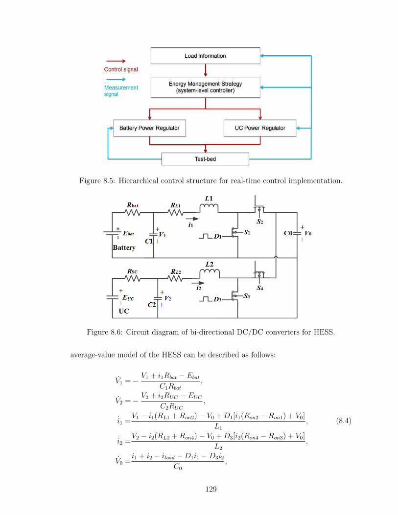
Figure 8.5: Hierarchical control structure for real-time control implementation.
Figure 8.6: Circuit diagram of bi-directional DC/DC converters for HESS.
average-value model of the HESS can be described as follows:
V1 =− V1 + i1Rbat − Ebat
C1Rbat
,
V2 =− V2 + i2RUC − EUC
C2RUC
,
i1 =V1 − i1(RL1 +Ron2)− V0 +D1[i1(Ron2 −Ron1) + V0]
L1
,
i2 =V2 − i2(RL2 +Ron4)− V0 +D3[i2(Ron4 −Ron3) + V0]
L2
,
V0 =i1 + i2 − iload −D1i1 −D3i2
C0
,
(8.4)
129

where C0 is the bus capacitor; C1, and C2 are the capacitors in parallel with the bat-
tery and UC, respectively; V0, V1 and V2 are the voltages corresponding to capacitors
C0, C1, and C2, respectively; L1, and L2 are the inductors of the bi-directional DC/DC
converters; i1 and i2 are the inductor currents; RL1, and RL2 are the resistance of
inductor L1 and L2, respectively; and D1 and D3 are the duty cycle commands of the
DC/DC converters.
As shown in Equation (8.4), the HESS with bi-directional converters is a non-
linear system, which requires a robust nonlinear approach. Sliding-mode control is
a robust nonlinear control approach, which has been successfully applied to robot
manipulators, vehicles, high-performance electric motors, and power systems [98]. In
this chapter, the sliding-mode control is used to control the bi-directional DC/DC
converters [69]. The sliding surface is defined as S = [S1, S2]T , where S1 = i1ref − i1
and S2 = i2ref − i2.
In order to ensure the existence of the sliding-mode surface, the condition SS < 0
must be satisfied. The differential sliding variable is set as:
S = −kS − εsat(S), (8.5)
where the saturation function sat(S) is defined as:
sat(Sn) =
1, Sn ∈ (1,∞),
Sn, Sn ∈ [−1, 1],
−1, Sn ∈ (−∞,−1),
(8.6)
n = 1, 2, k and ε are the sliding-mode gains.
To simplify the solution, we assume that Ron1 = Ron2 and Ron3 = Ron4. Assuming
a time scale separation (i.e., the current dynamic is much faster than the voltage
dynamic due to large values for the capacitances C0, C1, and C2), the voltages V0,1,2
130
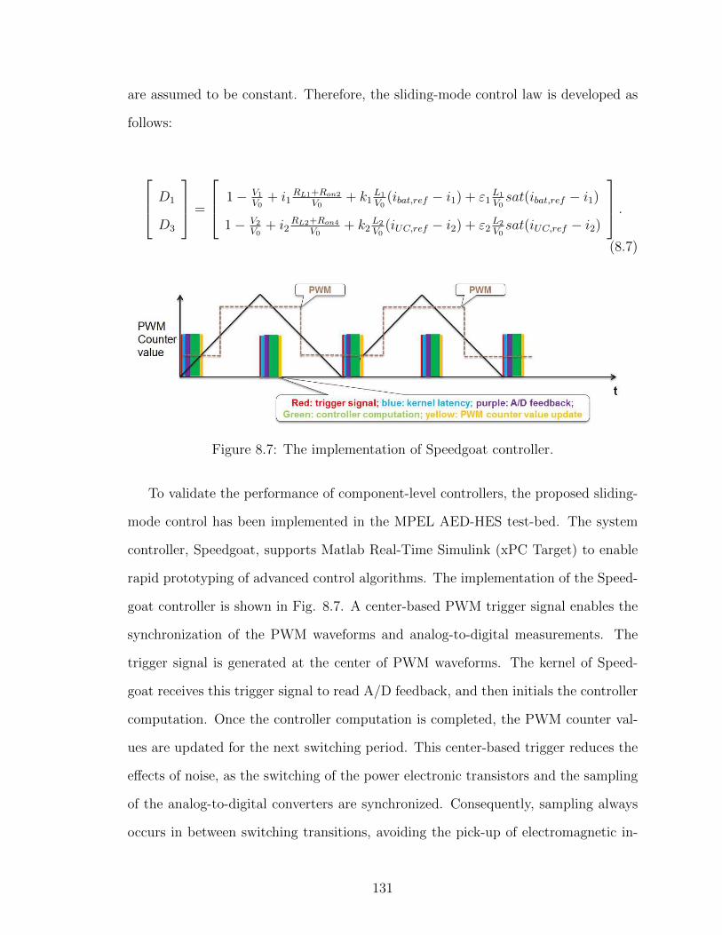
are assumed to be constant. Therefore, the sliding-mode control law is developed as
follows:
D1
D3
=
1− V1
V0+ i1
RL1+Ron2
V0+ k1
L1
V0(ibat,ref − i1) + ε1
L1
V0sat(ibat,ref − i1)
1− V2
V0+ i2
RL2+Ron4
V0+ k2
L2
V0(iUC,ref − i2) + ε2
L2
V0sat(iUC,ref − i2)
.(8.7)
Figure 8.7: The implementation of Speedgoat controller.
To validate the performance of component-level controllers, the proposed sliding-
mode control has been implemented in the MPEL AED-HES test-bed. The system
controller, Speedgoat, supports Matlab Real-Time Simulink (xPC Target) to enable
rapid prototyping of advanced control algorithms. The implementation of the Speed-
goat controller is shown in Fig. 8.7. A center-based PWM trigger signal enables the
synchronization of the PWM waveforms and analog-to-digital measurements. The
trigger signal is generated at the center of PWM waveforms. The kernel of Speed-
goat receives this trigger signal to read A/D feedback, and then initials the controller
computation. Once the controller computation is completed, the PWM counter val-
ues are updated for the next switching period. This center-based trigger reduces the
effects of noise, as the switching of the power electronic transistors and the sampling
of the analog-to-digital converters are synchronized. Consequently, sampling always
occurs in between switching transitions, avoiding the pick-up of electromagnetic in-
131

Figure 8.8: Matlab/Simulink program of the local controllers.
terference caused by the transitions. Center-based sampling is also able to measure
the average value of the inductor current. However, due to hardware delays, a phase
shift can cause measurement errors, which can be significant when the value of the
measurement is small. Our double-sampling method, which samples twice within one
switching period, can achieve more accurate average feedback. The Matlab/Simulink
code is developed as shown in Fig. 8.8. As shown in Fig. 8.9, the actual output
power of the HESS can follow the power reference quite accurately.
8.4 Experimental Implementation and Performance Evalua-
tion
In addition to the efficient optimization algorithm described in the previous sec-
tion, parallel computing using a multi-core structure can also increase the compu-
tational capabilities of our system [99, 100]. In this experiment, the system-level
controller is executed in core 1, while the component-level controllers are executed in
core 2. Both system-level and component-level controllers are synchronized with the
center-based trigger signal. The multi-core structure in Matlab/Simulink is shown
in Figure 8.10. A real-time simulation is performed to evaluate the computational
132

0 10 20 30 40time (sec)
-2000
-1000
0
1000
2000
Pow
er (
W)
Battery Power CommandBattery Power
0 10 20 30 40time (sec)
-2000
-1000
0
1000
2000
Pow
er (
W)
Cap Power CommandCap Power
time (sec)18 20 22 24 26 28 30
Pow
er (
W)
-2000
-1000
0
1000
2000Battery Power CommandBattery Power
time (sec)18 20 22 24 26 28 30
Pow
er (
W)
-2000
-1000
0
1000
2000
Cap Power CommandCap Power
Figure 8.9: Control performance: battery and UC command power and actual power(zoom-in plots in the bottom).
capability of our proposed hierarchical real-time MPC. As shown in Figures 8.11 and
8.12, the maximum execution time for both cores 1 and 2 are much smaller than their
corresponding sampling times.
In this experiment, the maximum voltage and the desired reference voltage of UC
are defined as 150V and 145V, respectively. The maximum and minimum output
currents of the battery and UC are 30A and -30A, respectively. The load fluctuations
are scaled to a peak value of 2kW. Uncertainties, such as load uncertainties, parameter
uncertainties, modeling uncertainties, and measurement uncertainties, exist in the
system and can be used to evaluate the robustness of the proposed controller. A
diagram of this experimental setup is shown in Fig. 8.13. A three-phase diode rectifier
converts the AC power from the grid to DC power, and then a DC/DC converter
133

Figure 8.10: Multi-core structure of Speedgoat.
Figure 8.11: Real-time simulation evaluation of system-level controller (core1).
Figure 8.12: Real-time simulation evaluation of component-level controllers (core2).
“bucks” the DC voltage down to the nominal voltage. We note that a constant duty
cycle is used for this DC/DC converter. In order to emulate the generator sets, the
second DC/DC converter is controlled to provide the average power for the DC bus.
The resistive load bank is controlled to emulate the load fluctuations by using the
134

propulsion-load model described in Chapter II. The HESS compensates the load
fluctuations to maintain a constant DC bus voltage. The predictive horizon is chosen
to be N=20. The experimental results of the filter-based and real-time MPC strategies
are shown in Figs. 8.14 (sea state 4) and 8.15 (sea state 6).
The pulse power load is another important load fluctuation in the shipboard net-
work. In the following experiments, we also evaluate the capability of the proposed
HESS solution to address the propulsion load fluctuations with pulse power loads,
as shown in Fig. 8.16. The following normalized performance metrics are used to
compare the real-time MPC with the filter-based strategy:
1. Voltage variation (Vol%):rms(V busMPC−V busref )
rms(V busfilter−V busref )× 100%;
2. Estimated HESS losses (HESS%): LossesMPC
Lossesfilter× 100%;
3. Battery peak current (Peak%):max(|IB,MPC |)max(|IB,filter|)
× 100%;
4. Battery RMS current (RMS%):rms(IB,MPC)
rms(IB,filter)× 100%.
Table 8.1: Performance comparison: filter-based vs. MPC.SS4 SS6 SS4 with Pulse
Vol% 61.96% 63.95% 71.10%HESS% 34.05% 49.77% 35.82%Peak% 51.11% 67.35% 53.50%RMS% 40.99% 64.19% 50.36%
As shown in Table 8.1, compared with the filter-based strategy, the proposed
real-time MPC can reduce the bus voltage variation to as low as 62% of the filter-
based approach, and HESS total losses are reduced as low as 35% of the filter-based
approach. Furthermore, the real-time MPC operates with much smaller battery peak
and RMS currents than the filter-based strategy, leading to an extended battery life
cycle. As shown in Figs. 8.14 - 8.16, the UC is operating around the desired reference
voltage under the real-time MPC strategy, while the voltage of UC keeps decreasing
under the filter-based strategy. The efficiency of the filter-based strategy will decrease
135

Figure 8.13: Diagram of real-time MPC experiment.
0 50 100 150-2000
0
2000
Pow
er (
W)
Filter-based EMS
Load Power Fluctuation
0 50 100 150196
198
200
202
204
Vol
tage
(V
) Bus Voltage
0 50 100 150140
142
144
146
Vol
tage
(V
)
UC Voltage
0 50 100 150
time (sec)
-10
0
10
Cur
rent
(A
)
UC CurrentB Current
0 50 100 150-2000
0
2000MPC-based EMS (N=20)
Load Power Fluctuation
0 50 100 150196
198
200
202
204Bus Voltage
0 50 100 150140
142
144
146
UC Voltage
0 50 100 150
time (sec)
-10
0
10
UC CurrentB Current
Figure 8.14: Experimental results of sea state 4: MPC vs. filter-based control
136
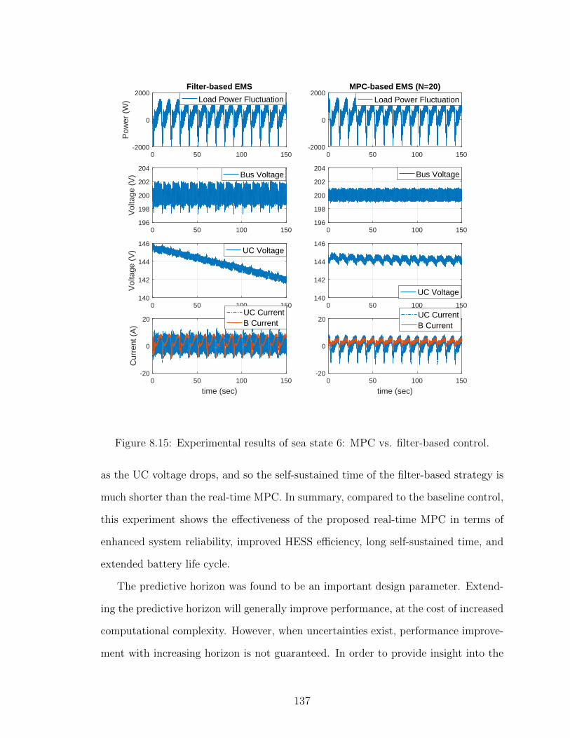
0 50 100 150-2000
0
2000
Pow
er (
W)
Filter-based EMS
Load Power Fluctuation
0 50 100 150196
198
200
202
204
Vol
tage
(V
) Bus Voltage
0 50 100 150140
142
144
146
Vol
tage
(V
) UC Voltage
0 50 100 150
time (sec)
-20
0
20
Cur
rent
(A
)
UC CurrentB Current
0 50 100 150-2000
0
2000MPC-based EMS (N=20)
Load Power Fluctuation
0 50 100 150196
198
200
202
204Bus Voltage
0 50 100 150140
142
144
146
UC Voltage
0 50 100 150
time (sec)
-20
0
20UC CurrentB Current
Figure 8.15: Experimental results of sea state 6: MPC vs. filter-based control.
as the UC voltage drops, and so the self-sustained time of the filter-based strategy is
much shorter than the real-time MPC. In summary, compared to the baseline control,
this experiment shows the effectiveness of the proposed real-time MPC in terms of
enhanced system reliability, improved HESS efficiency, long self-sustained time, and
extended battery life cycle.
The predictive horizon was found to be an important design parameter. Extend-
ing the predictive horizon will generally improve performance, at the cost of increased
computational complexity. However, when uncertainties exist, performance improve-
ment with increasing horizon is not guaranteed. In order to provide insight into the
137

0 5 10 15 20 25 30-2000
0
2000
Pow
er (
W)
Filter-based EMS
Load Power Fluctuation
0 50 100 150194
196
198
200
202
204
Vol
tage
(V
) Bus Voltage
0 50 100 150138
140
142
144
146
Vol
tage
(V
) UC Voltage
0 50 100 150
time (sec)
-10
0
10
20
Cur
rent
(A
)
UC CurrentB Current
0 5 10 15 20 25 30-2000
0
2000MPC-based EMS (N=20)
Load Power Fluctuation
0 50 100 150194
196
198
200
202
204Bus Voltage
0 50 100 150138
140
142
144
146UC Voltage
0 50 100 150
time (sec)
-10
0
10
20
UC CurrentB Current
Figure 8.16: Experimental results of pulse power load: MPC vs. filter-based control.
predictive horizon, the real-time MPC with an extended predictive horizon N=40 is
implemented on the testbed. The experimental results are shown in Figs.8.17 - 8.19.
The normalized performance metrics are presented as follows:
1. Voltage variation (Vol%):rms(V busN=40−V busref )
rms(V busN=20−V busref )× 100%;
2. HESS losses (HESS%): LossesN=40
LossesN=20× 100%;
3. Battery peak current (Peak%):max(|IB,N=40|)max(|IB,N=20|)
× 100%;
4. Battery RMS current (RMS%):rms(IB,N=40)
rms(IB,N=20)× 100%.
138

Table 8.2: Performance comparison: MPC(N=20) vs. MPC(N=40).SS4 SS6 SS4 with Pulse
Vol% 102.27% 100.52% 101.45%HESS% 101.86% 110.59% 98.55%Peak% 107.69% 107.67% 98.30%RMS% 105.94% 108.36% 100.44%
0 50 100 150-2000
0
2000
Pow
er (
W)
MPC-based EMS (N=40)
Load Power Fluctuation
0 50 100 150
200
205
Vol
tage
(V
)
Bus Voltage
0 50 100 150142
144
146
Vol
tage
(V
)
UC Voltage
0 50 100 150
time (sec)
-10
0
10
Cur
rent
(A
)
UC CurrentB Current
0 50 100 150-2000
0
2000MPC-based EMS (N=20)
Load Power Fluctuation
0 50 100 150
200
205Bus Voltage
0 50 100 150142
144
146
UC Voltage
0 50 100 150
time (sec)
-10
0
10
UC CurrentB Current
Figure 8.17: Experimental results of sea state 4: MPC(N=20) vs. MPC(N=40).
As shown in Table 8.2, MPC with N=40 does not outperform MPC with N=20
in most performance metrics. The real-time MPC only applies the first element of
the control sequence as the control action before moving to the next sample, when
new measurements are collected and the optimization is repeated with new initial
conditions. This feedback mechanism is helpful to improve the robustness of the MPC
strategy. However, as the predictive horizon increases, it is seen that uncertainties
can affect the control performance more significantly than a short predictive horizon.
In this study, therefore, the predictive horizon was chosen to be N=20.
Remark 8.1 As shown in Equation (8.1), this is nonlinear and nonconvex opti-
139

0 50 100 150-2000
0
2000
Pow
er (
W)
MPC-based EMS (N=40)
Load Power Fluctuation
0 50 100 150196
198
200
202
204
Vol
tage
(V
)
Bus Voltage
0 50 100 150142
144
146
Vol
tage
(V
)
UC Voltage
0 50 100 150
time (sec)
-10
0
10
Cur
rent
(A
)
UC CurrentB Current
0 50 100 150-2000
0
2000MPC-based EMS (N=20)
Load Power Fluctuation
0 50 100 150196
198
200
202
204 Bus Voltage
0 50 100 150142
144
146
UC Voltage
0 50 100 150
time (sec)
-10
0
10
UC CurrentB Current
Figure 8.18: Experimental results of sea state 6: MPC(N=20) vs. MPC(N=40).
mization problem. To solve this optimization problem is a challenge for implementing
the proposed MPC-based EMS in real-time applications. In this experiment, the out-
put currents of HESS do not reach their corresponding physical constraints, namely
-30A and 30A. It is important to understand the impact of constraints on solving the
optimization problem, so a new real-time simulation case study is performed. The
constraint of UC output current is changed from [−30A, 30A] to [−5A, 5A], and sea
state 6 load profile is used. In this case study, the real-time simulation results are
shown in Figure 8.20, where the UC current is always within its constraints. Fur-
thermore, the iteration to solve the optimization problem is significantly increased
when the UC current reaches its constraint. For example, the iteration is less than
15 (minimum: 3 times; maximum: 14 times) from 9 second to 11 second, while the
iteration can be as high as 30 when the constraint is active, such as from 4 second
to 6 second. The maximum execution time are shown in Figure 8.21 to validate the
140

0 5 10 15 20 25 30-2000
0
2000
Pow
er (
W)
MPC-based EMS (N=40)
Load Power Fluctuation
0 50 100 150194196198200202204
Vol
tage
(V
) Bus Voltage
0 50 100 150142
144
146
Vol
tage
(V
) UC Voltage
0 50 100 150
time (sec)
-10
0
10
Cur
rent
(A
)
UC CurrentB Current
0 5 10 15 20 25 30-2000
0
2000MPC-based EMS (N=20)
Load Power Fluctuation
0 50 100 150194196198200202204 Bus Voltage
0 50 100 150142
144
146 UC Voltage
0 50 100 150
time (sec)
-10
0
10
UC CurrentB Current
Figure 8.19: Experimental results of pulse power load: MPC(N=20) vs. MPC(N=40)
2 4 6 8 10
Cu
rren
t (A
)
-5
0
5
UC Current
time (sec)2 4 6 8 10
Iter
atio
n
0
20
40Iteration
Figure 8.20: UC output current and the number of iteration to solve the optimizationproblem.
141

Figure 8.21: Real-time simulation comparison of maximum execution time.
real-time feasibility when the constraint is active. The blue and red bars represent
the maximum execution time with the UC current constraint as [−30A, 30A] and
[−5A, 5A], respectively. The green bar represents the sample time. As shown in Fig-
ure 8.21, although the computational time is increased when the constraint is active,
it is still much smaller than its sample time.
8.5 Summary
In this chapter, the proposed real-time MPC has been implemented on the AED-
HES testbed. In order to achieve real-time feasibility, three different efforts have
been made: properly formulating the optimization problem, identifying an efficient
optimization solver, and implementing the controller with a multi-core structure.
Furthermore, effective HESS component current regulators using sliding-mode con-
trol have been developed and validated. Compared to the filter-based control, the
proposed MPC demonstrated on the testbed can achieve superior performance in
terms of reduced bus voltage variation, battery peak and RMS currents, and HESS
losses. Given the uncertainties in the testbed, the robustness of the proposed MPC
is also demonstrated.
142

CHAPTER IX
Conclusions and Future Work
9.1 Conclusions
This research has focused on the modeling, analysis, and control of an electric
ship propulsion system with hybrid energy storage system (HESS), aiming at miti-
gating the effect of the propulsion load fluctuations. The tools development, namely
modeling and testbed development, are presented in Chapter II and III, respectively.
The feasibilities and effectiveness of HESS have been investigated in Chapter IV and
V. Two energy management strategies (EMSs) have been proposed and analyzed
with simulation results presented in Chapter VI. In Chapter VII, the propulsion
load torque estimation and prediction that are needed to implement model predic-
tive control (MPC) have been addressed by two approaches: adaptive load estima-
tion/prediction with model predictive control and input observer with linear predic-
tion. The real-time MPC is implemented on the test-bed in Chapter VIII. Compared
to the filter-based strategy, the experimental results demonstrate the effectiveness of
the proposed real-time MPC.
The main work and results are summarized as follows:
• Developed a control-oriented model for an all-electric ship propulsion system
with hybrid energy storage. This model included a propeller and ship dynamic
143

model, hybrid energy storage models, a diesel engine and generator set model,
a electrical motor model and a DC bus dynamic model. The propeller and ship
dynamic model is the main contribution, which captured both high- and low-
frequency load fluctuations on the propeller. The in-and-out-of-water effect are
also taken into consideration in this model.
• Developed a hardware test-bed in order to support and demonstrate model-
ing and control solutions on a hardware platform. This test-bed included a
system-level controller that can simultaneously control all of the power elec-
tronic converters interfacing with the HESS. My contributions to the test-bed
development include the system controller, energy storages and DC/DC convert-
ers. Two preliminary experimental results, i.e., battery with UCs and flywheel
with UCs, were presented to demonstrate the capabilities of the test-bed in
control implementation and system integration for electric drive systems with
HESS.
• Investigated the feasibility and effectiveness of different hybrid energy storage
system configurations, namely battery combined with ultra-capacitor (B/UC)
and battery with flywheel (B/FW), to mitigate load fluctuations. Dynamic
programming was used to obtain the global optimal solutions. These global
optimal solutions formed the basis of a comparative study of B/FW and B/UC
HESS, where the Pareto fronts of these two technologies at different sea state
(SS) conditions were derived. The analysis aimed to provide insights into the
advantages and limitations of each HESS solution.
• Two MPC-based control strategies, coordinated model predictive control (CC-
MPC) and pre-filtered model predictive control (PF-MPC), were designed and
evaluated. The results indicated that the CC-MPC strategy outperforms the
PF-MPC strategy in terms of power tracking, HESS efficiency, and self-sustained
144

operation time. A sensitivity analysis of the predictive horizon for the coordi-
nated control showed the feasibility of MPC-based strategies for real-time ap-
plications. This study provided insights into the importance of the coordination
of HESS.
• Developed two energy management strategies based on different integration
configurations, namely “plug-in” and “integrated”. For the “plug-in” approach,
different strategies were investigated to address the effect of the load fluctuation
in the electric ship propulsion system. Model-based analysis was performed to
understand the interactions between HESS and generator control systems. To
validate the interaction analysis and evaluate the benefits or limitations for each
strategy, a comparative study was performed. Results showed that the proposed
energy management system, i.e., the coordinated HESS EMS, is more effective in
improving the system efficiency and reliability than other strategies. This work
illustrated that a properly coordinated control is critical when introducing HESS
into an existing electric ship propulsion system. For the “integrated” approach,
a new energy management strategy was proposed to integrate power generation,
electric motor, and hybrid energy storage control for electric ship propulsion
systems in order to address the effects of power fluctuations in the shipboard
network. Simulation results showed that the proposed strategy is effective at
improving system efficiency, enhancing reliability, and reducing mechanical wear
and tear.
• Developed two approaches to address propeller-load torque estimation and pre-
diction. The first combined an input observer with linear prediction, and the
second integrated parameter identification with model predictive control. A
comparative study was performed to illustrate the effectiveness of the proposed
model-based approach. The importance of load torque estimation and predic-
145

tion was also determined through this comparative study.
• The real-time MPC was implemented on the physical testbed. Three different
efforts have been made to enable real-time feasibility: a specially tailored prob-
lem formulation, an efficient optimization algorithm and a multi-core hardware
implementation. Component-level control was also developed to guarantee the
system-level control performance. Compared to the filter-based control strat-
egy, the proposed real-time MPC achieved much better performance in terms of
the enhanced system reliability, improved HESS efficiency, long self-sustained
time, and extended battery life cycle.
9.2 Ongoing and Future Research
Although substantial progress has been made on the modeling, analysis, optimiza-
tion, and control of all-electric ship propulsion systems with hybrid energy storage to
mitigate the impact of the propulsion load fluctuations, there are several ongoing and
future research topics to address open issues. These research activities are highlighted
in the following:
• Improve computational efficiency for solving the load-following optimization
problem with periodic load profiles
Propulsion-load fluctuations caused by the encounter waves and propeller ro-
tation have a periodic characteristic, which could potentially be exploited to
improve the computational efficiency and reduce the memory required for the
load-following optimization problem. How to take advantage of this periodic
characteristic is an ongoing research problem.
• Energy management strategy implementation for integrated approach
146

The energy management strategy for the plug-in approach has been imple-
mented on the testbed and achieves desired performance. The EMS for the
integrated approach requires more efforts on both system-level control and
component-level control, as well as the hardware. The experimental validation
of EMS for the integrated approach will be performed in the future research.
147

BIBLIOGRAPHY
148

BIBLIOGRAPHY
[1] Norbert Doerry. Naval power systems: Integrated power systems for the conti-nuity of the electrical power supply. IEEE Electrification Magazine, 3(2):12–21,2015.
[2] Torstein Ingebrigtsen Bø. Scenario-and Optimization-Based Control of MarineElectric Power Systems. PhD thesis, Norwegian University of Science and Tech-nology, 2016.
[3] Bijan Zahedi, Lars E Norum, and Kristine B Ludvigsen. Optimized efficiencyof all-electric ships by dc hybrid power systems. Journal of power sources,255:341–354, 2014.
[4] John Kuseian. Naval power systems technology development roadmap. ElectricShips Office, PMS, 320, 2013.
[5] Hyeongjun Park. Real-time predictive control of constrained nonlinear systemsusing the ipa-sqp approach. 2014.
[6] Espen Skjong, Rune Volden, Egil Rødskar, Marta Molinas, Tor Arne Johansen,and Joseph Cunningham. Past, present, and future challenges of the marinevessels electrical power system. IEEE Transactions on Transportation Electri-fication, 2(4):522–537, 2016.
[7] Timothy J McCoy. Trends in ship electric propulsion. In Power EngineeringSociety Summer Meeting, 2002 IEEE, volume 1, pages 343–346. IEEE, 2002.
[8] Alf Kare Adnanes. Maritime electrical installations and diesel electric propul-sion. ABB, 2003.
[9] Bijan Zahedi. Shipboard DC Hybrid Power Systems: Modeling, efficiency anal-ysis and stability control. PhD thesis, Norwegian University of Science andTechnology, 2014.
[10] Timothy J McCoy. Electric ships past, present, and future [technology leaders].IEEE Electrification Magazine, 3(2):4–11, 2015.
[11] Norbert Doerry, John Amy, and Cy Krolick. History and the status of electricship propulsion, integrated power systems, and future trends in the us navy.Proceedings of the IEEE, 103(12):2243–2251, 2015.
149

[12] Timothy J McCoy. Integrated power systemsan outline of requirements andfunctionalities for ships. Proceedings of the IEEE, 103(12):2276–2284, 2015.
[13] Norbert Doerry, Henry Robey, John Amy, and Chester Petry. Powering thefuture with the integrated power system. Naval Engineers Journal, 108(3):267–282, 1996.
[14] Herbert Ginn and Robert Cuzner. The shipboard integrated power system.IEEE Electrification Magazine, 1(2):2–3, 2015.
[15] So-Yeon Kim, Sehwa Choe, Sanggi Ko, and Seung-Ki Sul. A naval integratedpower system with a battery energy storage system: Fuel efficiency, reliability,and quality of power. IEEE Electrification Magazine, 3(2):22–33, 2015.
[16] Andrea Vicenzutti, Daniele Bosich, Giovanni Giadrossi, and Giorgio Sulligoi.The role of voltage controls in modern all-electric ships: Toward the all electricship. IEEE Electrification Magazine, 3(2):49–65, 2015.
[17] Gayathri Seenumani, Jing Sun, and Huei Peng. Real-time power managementof integrated power systems in all electric ships leveraging multi time scaleproperty. IEEE Transactions on Control Systems Technology, 20(1):232–240,2012.
[18] Norbert Doerry and Kevin McCoy. Next generation integrated power system:Ngips technology development roadmap. Technical report, DTIC Document,2007.
[19] Øyvind Notland Smogeli. Control of marine propellers: From normal to extremeconditions. PhD thesis, Norwegian University of Science and Technology, 2006.
[20] Damir Radan. Integrated control of marine electrical power systems. PhD thesis,Norwegian University of Science and Technology, 2008.
[21] Øyvind Notland Smogeli and Asgeir J Sørensen. Antispin thruster control forships. IEEE Transactions on Control Systems Technology, 17(6):1362–1375,2009.
[22] Øyvind N Smogeli, Asgeir J Sørensen, and Knut J Minsaas. The concept ofanti-spin thruster control. Control Engineering Practice, 16(4):465–481, 2008.
[23] Asgeir J Sørensen and Øyvind N Smogeli. Torque and power control of electri-cally driven marine propellers. Control Engineering Practice, 17(9):1053–1064,2009.
[24] Justin H McCarthy. On the calculation of thrust and torque fluctuations ofpropellers in nonuniform wake flow. Technical report, DTIC Document, 1961.
[25] John Carlton. Marine propellers and propulsion. Butterworth-Heinemann,2012.
150

[26] Kourosh Koushan et al. Dynamics of propeller blade and duct loadings onventilated thrusters in dynamic positioning mode. In Dynamic positioning con-ference. Houston, USA, 2007.
[27] RD Geertsma, RR Negenborn, K Visser, and JJ Hopman. Design and control ofhybrid power and propulsion systems for smart ships: A review of developments.Applied Energy, 194:30–54, 2017.
[28] Robert E Hebner, Kent Davey, John Herbst, David Hall, Jonathan Hahne,Dwayne D Surls, and Abdelhamid Ouroua. Dynamic load and storage integra-tion. Proceedings of the IEEE, 103(12):2344–2354, 2015.
[29] Srdjan M Lukic, Jian Cao, Ramesh C Bansal, Fernando Rodriguez, and AliEmadi. Energy storage systems for automotive applications. IEEE Transactionson industrial electronics, 55(6):2258–2267, 2008.
[30] Siang Fui Tie and Chee Wei Tan. A review of energy sources and energymanagement system in electric vehicles. Renewable and Sustainable EnergyReviews, 20:82–102, 2013.
[31] Joel R Anstrom, Benjamin Zile, Kandler Smith, H Hofmann, and A Batra.Simulation and field-testing of hybrid ultra-capacitor/battery energy storagesystems for electric and hybrid-electric transit vehicles. In Applied Power Elec-tronics Conference and Exposition, volume 1, pages 491–497, 2005.
[32] Micah Ortuzar, Jorge Moreno, and Juan Dixon. Ultracapacitor-based auxiliaryenergy system for an electric vehicle: Implementation and evaluation. IEEETransactions on industrial electronics, 54(4):2147–2156, 2007.
[33] Ziyou Song, Heath Hofmann, Jianqiu Li, Jun Hou, Xuebing Han, and MinggaoOuyang. Energy management strategies comparison for electric vehicles withhybrid energy storage system. Applied Energy, 134:321–331, 2014.
[34] Ziyou Song, Heath Hofmann, Jianqiu Li, Jun Hou, Xiaowu Zhang, and MinggaoOuyang. The optimization of a hybrid energy storage system at subzero temper-atures: Energy management strategy design and battery heating requirementanalysis. Applied Energy, 159:576–588, 2015.
[35] Ziyou Song, Jun Hou, Shaobing Xu, Minggao Ouyang, and Jianqiu Li. Theinfluence of driving cycle characteristics on the integrated optimization of hybridenergy storage system for electric city buses. Energy, 135:91–100, 2017.
[36] Francisco Dıaz-Gonzalez, Andreas Sumper, Oriol Gomis-Bellmunt, and RobertoVillafafila-Robles. A review of energy storage technologies for wind power ap-plications. Renewable and Sustainable Energy Reviews, 16(4):2154–2171, 2012.
[37] Sam Koohi-Kamali, VV Tyagi, NA Rahim, NL Panwar, and H Mokhlis. Emer-gence of energy storage technologies as the solution for reliable operation of
151

smart power systems: A review. Renewable and Sustainable Energy Reviews,25:135–165, 2013.
[38] Tarik Kousksou, Pascal Bruel, Abdelmajid Jamil, T El Rhafiki, and YoussefZeraouli. Energy storage: Applications and challenges. Solar Energy Materialsand Solar Cells, 120:59–80, 2014.
[39] Gaston Orlando Suvire, Marcelo Gustavo Molina, and Pedro Enrique Mercado.Improving the integration of wind power generation into ac microgrids usingflywheel energy storage. IEEE Transactions on smart grid, 3(4):1945–1954,2012.
[40] Jae-Do Park, Claude Kalev, and Heath F Hofmann. Control of high-speed solid-rotor synchronous reluctance motor/generator for flywheel-based uninterrupt-ible power supplies. IEEE Transactions on Industrial Electronics, 55(8):3038–3046, 2008.
[41] Wenjie Chen, Alf Kare Adnanses, Jan Fredrik Hansen, John Olav Lindtjørn,and Tianhao Tang. Super-capacitors based hybrid converter in marine electricpropulsion system. In Electrical Machines (ICEM), 2010 XIX InternationalConference on, pages 1–6. IEEE, 2010.
[42] Hyeongjun Park, Jing Sun, Steven Pekarek, Philip Stone, Daniel Opila, RichardMeyer, Ilya Kolmanovsky, and Raymond DeCarlo. Real-time model predictivecontrol for shipboard power management using the ipa-sqp approach. IEEETransactions on Control Systems Technology, 23(6):2129–2143, 2015.
[43] Saurabh Kulkarni and Surya Santoso. Impact of pulse loads on electric shippower system: With and without flywheel energy storage systems. In 2009IEEE Electric Ship Technologies Symposium, pages 568–573. IEEE, 2009.
[44] Lori N Domaschk, Abdelhamid Ouroua, Robert E Hebner, Oscar E Bowlin, andWB Colson. Coordination of large pulsed loads on future electric ships. IEEEtransactions on Magnetics, 43(1):450–455, 2007.
[45] Ahmed T Elsayed and Osama A Mohammed. Distributed flywheel energy stor-age systems for mitigating the effects of pulsed loads. In 2014 IEEE PESGeneral Meeting— Conference & Exposition, pages 1–5. IEEE, 2014.
[46] Ahmed T Elsayed and Osama A Mohammed. A comparative study on theoptimal combination of hybrid energy storage system for ship power systems.In 2015 Electric Ship Technologies Symposium (ESTS), pages 140–144. IEEE,2015.
[47] Torstein Ingebrigtsen Bø and Tor Arne Johansen. Battery power smoothingcontrol in a marine electric power plant using nonlinear model predictive control.IEEE Transactions on Control Systems Technology, 2016.
152

[48] Michel R Miyazaki, Asgeir J Sørensen, and Bjørn J Vartdal. Reduction offuel consumption on hybrid marine power plants by strategic loading with en-ergy storage devices. IEEE Power and Energy Technology Systems Journal,3(4):207–217, 2016.
[49] Yichao Tang and Alireza Khaligh. On the feasibility of hybrid bat-tery/ultracapacitor energy storage systems for next generation shipboard powersystems. In 2010 IEEE Vehicle Power and Propulsion Conference, pages 1–6.IEEE, 2010.
[50] Ali Haseltalab, Rudy R Negenborn, and Gabriel Lodewijks. Multi-level pre-dictive control for energy management of hybrid ships in the presence of un-certainty and environmental disturbances. IFAC-PapersOnLine, 49(3):90–95,2016.
[51] Jun Hou, Jing Sun, and Heath Hofmann. Mitigating power fluctuations inelectric ship propulsion with hybrid energy storage system: Design and anal-ysis. IEEE Journal of Oceanic Engineering, 2017, to be published. [Online].Available: http://ieeexplore.ieee.org/document/7887693/.
[52] Jun Hou, Jing Sun, and Heath Hofmann. Mitigating power fluctuations inelectrical ship propulsion using model predictive control with hybrid energystorage system. In 2014 American Control Conference, pages 4366–4371. IEEE,2014.
[53] Jun Hou, Jing Sun, and Heath Hofmann. Battery/flywheel hybrid energy stor-age to mitigate load fluctuations in electric ship propulsion systems. In 2017American Control Conference (ACC), pages 1296–1301. IEEE, 2017.
[54] Jun Hou, Jing Sun, and Heath Hofmann. Interaction analysis and integratedcontrol of hybrid energy storage and generator control system for electric shippropulsion. In 2015 American Control Conference (ACC), pages 4988–4993.IEEE, 2015.
[55] Jun Hou, Jing Sun, and Heath Hofmann. Integrated control of power generation,electric motor and hybrid energy storage for all-electric ships. In 2016 AmericanControl Conference (ACC), pages 6797–6802. IEEE, 2016.
[56] Jing Sun. Optimisation-based control for electrified vehicles: challenges andopportunities. Journal of Control and Decision, 2(1):46–63, 2015.
[57] Philip Stone, Daniel F Opila, Hyeongjun Park, Jing Sun, Steve Pekarek, RayDeCarlo, Eric Westervelt, James Brooks, and Gayathri Seenumani. Shipboardpower management using constrained nonlinear model predictive control. In2015 Electric Ship Technologies Symposium (ESTS), pages 1–7. IEEE, 2015.
[58] Pengfei Liu, Mohammed Islam, and Brian Veitch. Some unsteady propulsivecharacteristics of a podded propeller unit under maneuvering operation. In
153

Proceedings of the First International Symposium on Marine Propulsors-smp09,pages 507–516, 2009.
[59] Tristian Perez, Øyvind N Smogeli, Thor I Fossen, and Asgeir J Sørensen. Anoverview of the marine systems simulator (mss): A simulink R© toolbox for ma-rine control systems. Modeling, identification and Control, 27(4):259–275, 2006.
[60] Tor A Johansen, Torstein I Bø, Eirik Mathiesen, Aleksander Veksler, and As-geir J Sørensen. Dynamic positioning system as dynamic energy storage ondiesel-electric ships. IEEE Transactions on Power Systems, 29(6):3086–3091,2014.
[61] Damir Radan, Asgeir J Sørensen, Alf Kare Adnanes, and Tor A Johansen.Reducing power load fluctuations on ships using power redistribution control.Marine Technology, 45(3):162–174, 2008.
[62] Aleksander Veksler, Tor Arne Johansen, and Roger Skjetne. Thrust allocationwith power management functionality on dynamically positioned vessels. In2012 American Control Conference (ACC), pages 1468–1475. IEEE, 2012.
[63] Jun Hou, David M Reed, Kan Zhou, Heath Hofmann, and Jing Sun. Model-ing and test-bed development for an electric drive system with hybrid energystorage. In Electric Machines Technology Symposium, 2014.
[64] Jun Hou, David M Reed, Heath Hofmann, and Jing Sun. A low-voltage test-bedfor electric ship propulsion systems with hybrid energy storage. In AdvancedMachinery Technology Symposium (AMTS). ASNE, 2016.
[65] Jun Hou, David M Reed, Heath Hofmann, and Jing Sun. A low-voltage test-bedfor electric ship propulsion systems with hybrid energy storage. Naval EngineersJournal, 2017, under review.
[66] Jun Hou, Jing Sun, and Heath Hofmann. Control development and performanceevaluation for battery/flywheel hybrid energy storage solutions to mitigate loadfluctuations in all-electric ship propulsion systems. 2017, under review.
[67] Jun Hou, Ziyou Song, Hyeongjun Park, Jing Sun, and Heath Hofmann. Real-time model predictive control for load fluctuations mitigation in all-electric shippropulsion systems. 2017, under preparation.
[68] Jun Hou, Jing Sun, and Heath Hofmann. Adaptive mpc with propulsion loadestimation and prediction for all-electric ship energy management. 2017, underreview.
[69] Ziyou Song, Jun Hou, Heath Hofmann, Jianqiu Li, and Minggao Ouyang.Sliding-mode and lyapunov function-based control for battery/supercapacitorhybrid energy storage system used in electric vehicles. Energy, 122:601–612,2017.
154

[70] MM Barnitsas, D Ray, and P Kinley. Kt, kq and efficiency curves for thewageningen b-series propellers. Technical report, University of Michigan, 1981.
[71] HydroComp. Correlating propeller performance with kt/kq multipliers. Tech-nical report, HydroComp, Inc., 2003.
[72] Kenneth John Rawson. Basic ship theory, volume 1. Butterworth-Heinemann,2002.
[73] Zhen Li. Path following with roll constraints for marine surface vessels in wavefields. PhD thesis, The University of Michigan, 2009.
[74] R.L. Beck and J. Wolfe. Developing a ship motions prediction program us-ing linear theory for a ship maneuvering through a seaway. Technical report,Technical Report, 2007.
[75] D. Peng. Propeller design report. Technical report, Technical Report, 2009.
[76] Min Chen and Gabriel A Rincon-Mora. Accurate electrical battery model ca-pable of predicting runtime and iv performance. IEEE transactions on energyconversion, 21(2):504–511, 2006.
[77] Petar J Grbovic. Ultra-capacitors in power conversion systems: analysis, mod-eling and design in theory and practice. John Wiley & Sons, 2013.
[78] Reed T Doucette and Malcolm D McCulloch. A comparison of high-speedflywheels, batteries, and ultracapacitors on the bases of cost and fuel economyas the energy storage system in a fuel cell based hybrid electric vehicle. Journalof Power Sources, 196(3):1163–1170, 2011.
[79] Dongxiang Yan, Languang Lu, Zhe Li, Xuning Feng, Minggao Ouyang, andFachao Jiang. Durability comparison of four different types of high-powerbatteries in hev and their degradation mechanism analysis. Applied Energy,179:1123–1130, 2016.
[80] Eduardo F Camacho and Carlos Bordons Alba. Model predictive control.Springer Science & Business Media, 2013.
[81] David Q Mayne. Model predictive control: Recent developments and futurepromise. Automatica, 50(12):2967–2986, 2014.
[82] M Bash, RR Chan, J Crider, C Harianto, J Lian, J Neely, SD Pekarek, SD Sud-hoff, and N Vaks. A medium voltage dc testbed for ship power system research.In 2009 IEEE Electric Ship Technologies Symposium (ESTS), 2009.
[83] Jorge Solsona, Maria I Valla, and Carlos Muravchik. Nonlinear control of a per-manent magnet synchronous motor with disturbance torque estimation. IEEETransactions on Energy Conversion, 15(2):163–168, 2000.
155

[84] Chia-Shang Liu and Huei Peng. Disturbance observer based tracking control.Journal of Dynamic Systems, Measurement, and Control, 122(2):332–335, 2000.
[85] Ilya Kolmanovsky, Irina Sivergina, and Jing Sun. Simultaneous input and pa-rameter estimation with input observers and set-membership parameter bound-ing: theory and an automotive application. International Journal of AdaptiveControl and Signal Processing, 20(5):225–246, 2006.
[86] Wen-Hua Chen, Jun Yang, Lei Guo, and Shihua Li. Disturbance-observer-based control and related methodsan overview. IEEE Transactions on IndustrialElectronics, 63(2):1083–1095, 2016.
[87] PP Vaidyanathan. The theory of linear prediction. Synthesis lectures on signalprocessing, 2(1):1–184, 2007.
[88] Petros A Ioannou and Jing Sun. Robust adaptive control, 2012.
[89] R. Ghaemi. Robust model based control of constrained systems. PhD thesis,The University of Michigan, 2010.
[90] Hyeongjun Park, Jing Sun, and Ilya Kolmanovsky. A tutorial overview of ipa-sqp approach for optimization of constrained nonlinear systems. In IntelligentControl and Automation (WCICA), 2014 11th World Congress on, pages 1735–1740. IEEE, 2014.
[91] Marco Cupelli, Ferdinanda Ponci, Giorgio Sulligoi, Andrea Vicenzutti, Chris SEdrington, Touria El-Mezyani, and Antonello Monti. Power flow control andnetwork stability in an all-electric ship. Proceedings of the IEEE, 103(12):2355–2380, 2015.
[92] Luis Herrera, Wei Zhang, and Jin Wang. Stability analysis and controller designof dc microgrids with constant power loads. IEEE Transactions on Smart Grid,8(2):881–888, 2017.
[93] Noshin Omar, Mohamed Abdel Monem, Yousef Firouz, Justin Salminen, JelleSmekens, Omar Hegazy, Hamid Gaulous, Grietus Mulder, Peter Van denBossche, Thierry Coosemans, et al. Lithium iron phosphate based battery–assessment of the aging parameters and development of cycle life model. AppliedEnergy, 113:1575–1585, 2014.
[94] Masoud Masih-Tehrani, Mohammad-Reza Ha’iri-Yazdi, Vahid Esfahanian, andAli Safaei. Optimum sizing and optimum energy management of a hybrid energystorage system for lithium battery life improvement. Journal of Power Sources,244:2–10, 2013.
[95] John Wang, Ping Liu, Jocelyn Hicks-Garner, Elena Sherman, Souren Souki-azian, Mark Verbrugge, Harshad Tataria, James Musser, and Peter Fi-namore. Cycle-life model for graphite-lifepo 4 cells. Journal of Power Sources,196(8):3942–3948, 2011.
156

[96] A. Bryson and Y. Ho. Applied optimal control: optimization, estimation, andcontrol. Taylor & Francis, 1975.
[97] Y. Xie, R. Ghaemi, J. Sun, and J. Freudenberg. Model predictive control for afull bridge dc/dc converter. IEEE Transactions on Control Systems Technology,20(1):164–172, 2012.
[98] Jean-Jacques E Slotine, Weiping Li, et al. Applied nonlinear control, volume199. Prentice hall Englewood Cliffs, NJ, 1991.
[99] Piotr Luszczek. Enhancing multicore system performance using parallel com-puting with matlab. MATLAB Digest, 17(5), 2008.
[100] Jeremy Kepner. Parallel MATLAB for multicore and multinode computers.SIAM, 2009.
157