control laws design and validation of autonomous mobile

17

Control Laws Design and Validation of Autonomous Mobile Robot Off-Road Trajectory Tracking Based on

ADAMS and MATLAB Co-Simulation Platform

Yang. Yi, Fu. Mengyin, Zhu. Hao and Xiong. Guangming School of Automation, Beijing Institute of Technology,

China

1. Introduction

Autonomous automobile technology is a rapidly developing field, with interest in both academia and industry. Outdoor navigation of autonomous vehicles, especially for rough-terrain driving, has already been a new research focus. DARPA Grand Challenge and LAGR program stand for the top development level in this research region. Rough-terrain driving research offers a challenge that the in-vehicle control system must be able to handle rough and curvy roads, and quickly varying terrain types, such as gravel, loose sand, and mud puddles – while stably tracking trajectories between closely spaced hazards. The vehicle must be able to recover from large disturbances, without intervention (Gabriel, 2007). Since robotics autonomous navigation tasks in outdoor environment can be effectively performed by skid-steering vehicles, these vehicles are being widely used in military affairs, academia research, space exploration, and so on. In reference (Luca, 1999), a model-based nonlinear controller is designed, following the dynamic feedback linearization paradigm. In reference (J.T. Economou, 2000), the authors applied experimental results to enable Fuzzy Logic modelling of the vehicle-ground interactions in an integrated manner. These results illustrate the complexity of systematic modeling the ground conditions and the necessity of using two variables in identifying the surface properties. In reference (Edward, 2001), the authors described relevant rover safety and health issues and presents an approach to maintaining vehicle safety in a navigational context. Fuzzy logic approaches to reasoning about safe attitude and traction management are presented. In reference (D. Lhomme-Desages, 2006), the authors introduced a model-based control for fast autonomous mobile robots on soft soils. This control strategy takes into account slip and skid effects to extend the mobility over planar, granular soils. Different from above researches, which control the robots on the tarmac, grass, sand, gravel or soil, this chapter focuses on the motion control for skid-steering vehicles on the bumpy and rocklike terrain, and presents novel and effective trajectory tracking control methods, including the longitudinal, lateral, and sensors pan-tilt control law. Furthermore, based on ADAMS&MATLAB co-simulation platform, iRobot ATRV2 is

www.intechopen.com

Applications of MATLAB in Science and Engineering

354

modelled and the bumpy off-road terrain is constructed, at the same time, trajectory tracking control methods are validated effectively on this platform.

2. Mobile robot dynamic analysis

To research on the motion of skid-steering robots, the 4-wheeled differentially driven robot,

which is moving on the horizontal road normally without longitudinal wheel slippage, is

analyzed for kinematics and dynamics. As shown in Fig. 1 (a), global Descartes frame and

in-vehicle Descartes frame are established. In Global frame OXYZ , its origin O is sited on

the horizontal plane where the robot is running, and Z axis is orthogonal to the plane; in in-

vehicle frame oxyz , its origin o is located at the robot center of mass, z axis is orthogonal

to the chassis of robot, x axis is parallel to the rectilinear translation orientation of the robot

and y axis is orthogonal to the translation orientation in the plane of the chassis. The robot

wheelbase is A and the distance between the left and right wheels is B . According to the

relation between OXYZ and oxyz , the kinematics equation is as follows.

cos sin cos sin

sin cossin cos

X x y x

x y yY

(1)

The derivative of equation (1) with respect to time is

cos sin

sin cos

cos sin

sin cos

x

y

X x y

Y y x

a

a

(2)

(a) (b)

Fig. 1. Dynamics analysis of the robot and the motion constraint about oC

www.intechopen.com

Control Laws Design and Validation of Autonomous Mobile Robot Off-Road Trajectory Tracking Based on ADAMS and MATLAB Co-Simulation Platform

355

In the above equations, , , ,X Y X Y represent the absolute longitudinal and lateral velocities, and

the absolute longitudinal and lateral accelerations respectively; is the angle between x

and X axes. , ,x y denote longitudinal, lateral and angular velocities in in-vehicle frame,

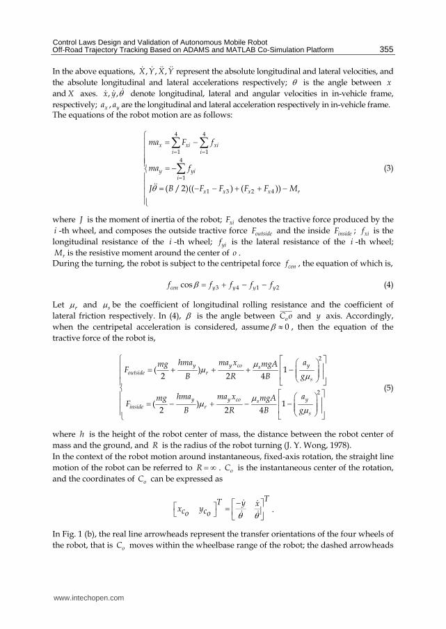
respectively; ,x ya a are the longitudinal and lateral acceleration respectively in in-vehicle frame. The equations of the robot motion are as follows:

4 4

1 1

4

1

1 3 2 4( / 2)(( ) ( ))

x xi xii i

y yii

x x x x r

ma F f

ma f

J B F F F F M

(3)

where J is the moment of inertia of the robot; xiF denotes the tractive force produced by the

i -th wheel, and composes the outside tractive force outsideF and the inside insideF ; xif is the

longitudinal resistance of the i -th wheel; yif is the lateral resistance of the i -th wheel;

rM is the resistive moment around the center of o . During the turning, the robot is subject to the centripetal force cenf , the equation of which is,

3 4 1 2coscen y y y yf f f f f (4)

Let r and s be the coefficient of longitudinal rolling resistance and the coefficient of

lateral friction respectively. In (4), is the angle between oC o

and y axis. Accordingly,

when the centripetal acceleration is considered, assume 0 , then the equation of the

tractive force of the robot is,

2

2

( ) 12 2 4

( ) 12 2 4

y y co ysoutside r

s

y y co ysinside r

s

hma ma x amg mgAF

B R B g

hma ma x amg mgAF

B R B g

(5)

where h is the height of the robot center of mass, the distance between the robot center of

mass and the ground, and R is the radius of the robot turning (J. Y. Wong, 1978).

In the context of the robot motion around instantaneous, fixed-axis rotation, the straight line

motion of the robot can be referred to R . oC is the instantaneous center of the rotation,

and the coordinates of oC can be expressed as

TT y xx yc co o

.

In Fig. 1 (b), the real line arrowheads represent the transfer orientations of the four wheels of

the robot, that is oC moves within the wheelbase range of the robot; the dashed arrowheads

www.intechopen.com


356

stand for the transfer orientations of the four wheels of the robot, when oC , that is oC ,

moves beyond the wheelbase range of the robot. Clearly, if oC moves out of the wheelbase

range, the lateral transfer orientations of four wheels are the same; as a result, the motion of

the robot will be out of control. The motion constraint is as follows,

sin cos 0 ( 2 )

X

l Y l A

(6)

where l is the distance from oC to y axis. According to Fig. 1 (a) and equation (5), it is

cos 2y sl Aa g that can be obtained. Therefore, the constraint of the motion, shown as

follow, is imperative.

2 2( ) or ( )s sx R g R g (7)

In this paper, a description of trajectory space (Matthew Spenko, 2006) is presented

according to the robot’s dynamic analysis, which is defined as the two-dimensional space of

the robot’s turning angular speed and longitudinal velocity longV , ( )longV x . This kind of

description is very useful during motion control. Consider inequalities (7): 2( ( )) /long sV t R g or 2( ( )) st R g , it is easy to get | ( )|long sV t gR or | ( )| /st g R ,

then take another constraint into consideration, longV R , now a figure of the robot’s

( , )V space (see Fig. 2.) can be obtained. The boundary curve in the figure satisfies

( ) ( )long sV t t g . When the robot’s ( , )V state is in the shadow region, that’s to say

( ) ( )long sV t t g , the robot is safe, which means the hazardous situation like side slippage

won’t occur. As a result, inequalities (7) is crucial for control decision making.

Fig. 2. The ( , )V space of motion control of the robot. (In this figure, 0.49s

and 29.8 /g m s )

www.intechopen.com


357

3. Trajectory tracking control laws design

Autonomous mobile robot achieves outdoor navigation by three processes, including the environment information acquired by the perception module, the control decision made by the planner module, and the motion plan performed by the motion control module (Gianluca, 2007). Consequently, for safe and accurate outdoor navigation it is vital to harmonize the three modules performance. In this paper, the emphasis is focused on the decision of control laws of the robot, and these controlled objects include the longitudinal velocity, the lateral velocity, and the angles of sensor pan-tilts. As shown in Fig. 3, in an off-road environment, the robot uses laser range finder (LRF) with one degree of freedom (DOF) pan-tilt (only tilt) to scan bumpy situation of the close front ground, on which the robot is moving, and employs stereo vision with two DOF pan-tilt to perceive drivable situation of far front ground. With the data accessed from laser and vision sensors, the passable path can be planned, and the velocities of left and right robot’s sides can be controlled to track the path, consequently, the robot off-road running is completed.

Fig. 3. Off-road driving of the robot

3.1 Longitudinal control law In this section, a kind of humanoid driving longitudinal control law based on fuzzy logic is proposed. First, the effect factors to the longitudinal velocity are classified. As shown in Fig. 4,

Fig. 4. The longitudinal control law of the robot

Trajectory Curvature Radius

Fuzzy Longitudinal

Control Law

Road Roughness

Sensor System Process Time

Velocity Requirement

www.intechopen.com


358

these factors include curvature radius of trajectory, road roughness, process time of sensors and speed requirement. Based on the four factors and the analysis of kinematics and dynamics, the longitudinal velocity equation can be given,

( ) ( ) ( ) ( )long cv c rr rough t sen v re reV r R T V V (8)

where longV is longitude velocity command, cv , rr , t and v are the weight factors of

the curvature radius of trajectory cr , road roughness roughR , processing time of sensors senT

and speed requirement reV respectively. The weight factors can vary within [0, 1] .

3.2 Lateral control law Autonomous vehicle off-road driving is a special control problem because mathematical models are highly complex and can’t be accurately linearized. Fuzzy logic control, however, is robust and efficient for non-linear system control (Gao Feng, 2009), and a well-tested method for dealing with this kind of system, provides good results, and can incorporate human procedural knowledge into control algorithms. Also, fuzzy logic lets us mimic human driving behavior to some extent (José E. Naranjo, 2007). Therefore, the paper has presented a kind of novel fuzzy lateral control law for the robot off-road running. Thereafter, the lateral control law is designed for the purpose of position tracking by adjusting navigation orientation to reduce position error. Definition: When the robot moves toward the trajectory, the orientation angle of the robot is positive, whichever of the two regions, namely left error region and right error region of the tracking position, the robot is in. When the robot moves against the trajectory, the angle is negative. When the robot motion is parallel to the trajectory, the angle is zero.

Fig. 5. Plots of membership functions of ed

and e

. The upper plot stands for ( )ed

. 0.1,0.1 is the range of the center region, ( ) 1.0ed

in this region. The lower plot

expresses ( )e

, which is indicated with triangle membership function. In this figure, the

colorful bands represent the continuous changing course of ed

.

In the course of trajectory tracking of the robot, position error de and orientation error e ,

which are the error values between the robot and the trajectory, are the inputs of the lateral

www.intechopen.com


359

controller. First, the error inputs, including the position error and the orientation error, are

pre-processed to improve steady precision of the trajectory tracking, and restrain oscillation

of that. The error E can be written as E E E , where E is the result of smoothing filter

about E , i.e.

1

iE e ni

i n ;

E forecasts the error produced in the next system sample time,

( )1

iE k e n i nei i

i n .

As a result,

(1 ) ( )1

iE k e n i nei i

i n , 4n , ( , )ei ei sk f x T ,

sT represents system sample time. Second, the error inputs, after being pre-processed, are

fuzzyfication-processed. As shown in Fig. 5, degree of membership ( )de and ( )e are

indicated in terms of triangle and rectangle membership functions:

Part One: the space of de is divided into LB , LS , MC , RS , RB . According to the result of

the de division, the phenotype rules of the lateral fuzzy control law hold.

Part Two: the space of e is also divided into LB , LS , MC , RS , RB . According to the

result of the e division, the recessive rules of the control law are obtained.

It is necessary to explain that the phenotype rules are the basis of the recessive rules, namely

each phenotype rule possesses a group of relevant recessive rules. Each phenotype rule has

already established their own expectation orientation angle e , that is to say the robot is

expected to run on this orientation angle, e , and this angle is the very center angle of this

group recessive rules. When the center angle, e , of each group of recessive rules is varying,

the division of e of each group recessive rules changes accordingly.

All of the control rules can be expressed as continuous functions: LBf , LSf , MCf , RSf , RBf ,

and, consequently, the global continuity of the control rules is established.

The functions, LBf , LSf , RSf , RBf , which express the rule functions of the

non center region of de , are as follows:

( )

et e e

t trs

k kk

T

(9)

In (9), e is the expectation tracking-angle in the current position-error region, and e is

monotonically increasing with de. e can be given by this formula

arctan de d

elong

k e

V , ( ) ( )

de DL d DL DS d DSk e k e k ,

www.intechopen.com


360

where DL stands for the large error region, including LB and RB , membership degree of

de , and DS represents the small error region, including LS and RS , membership degree

of de . tr is the estimation of the trajectory-angle rate. e

k can be worked out by this

equation:

( ) ( )e

L e L S e Sk k k ,

where L stands for the large error region, including LB and RB , membership degree of

e , and S denotes the small error region, including LS and RS , membership degree of

e . DLk and Lk express the standard coefficients of the large error region of de and e ;

DSk and Sk indicate the small error region of de and e , respectively. tk is the

proportional coefficients of the system sample time ST .

MCf is deduced as follows:

Fig. 6. Tracking trajectory of the robot. In this Figure, the red dashdotted line stands for the trajectory tracked by the robot. The different color dotted lines represent the bounderies of

the different error regions of de .

When the robot moves into the center region at the orientation of , the motion state of the

robot can be divided into two kinds of situations.

Situation One: Assume that has decreased into the rule admission angular range of center

region, i.e. 0 cent , where cent , which is subject to (7), is the critical angle of center

region. To make the robot approach the trajectory smoothly, the planner module requires

the robot to move along a certain circle path. As the robot moves along the circle path in Fig.

6, the values of de and e decrease synchronously. In Fig. 6, is the variety range of de in

the center region. is the angle between the orientation of the robot and the trajectory

when the robot just enters the center region. 22R can be worked out by geometry,

and in addition, the value of is very small, so the process of approaching trajectory can be

represented as

.

Situation Two: When 0 or cent . If the motion decision from the planner module

were the same as Situation One, the motion will not meet (7). According to the above

www.intechopen.com


361

analysis, the error of tracking can not converge until the adjusted e makes be true of

Situation One. Therefore, the purpose of control in Situation Two is to decrease e . Based on the above deduction, MCf is as follow:

( )t e e

t trs

kk

T

(10)

Where

d cente

e ,

is the variety range of de in the center region, 0.1 ,0 0,0.1m or m . is the output of (9)

and (10), at the same time, is subject to (7), consequently, 2 R gs

is required by the

control rules. The execution sequence of the control rules is as follows:

First, the phenotype control rules are enabled, namely to estimate which error region ( LB ,

LS , MC , RS , RB ) the current de of the robot belongs to, and to enable the relevant

recessive rules; Second, the relevant recessive rules are executed, at the same time, e is

established in time.

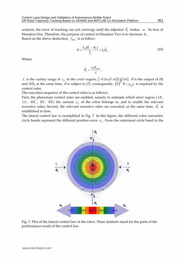
The lateral control law is exemplified in Fig. 7. In this figure, the different color concentric

circle bands represent the different position error de . From the outermost circle band to the

Fig. 7. Plot of the lateral control law of the robot. These dasheds stand for the parts of the performance result of the control law.

www.intechopen.com


362

center round, the values of de is decreasing. The red center round stands for MC of de ,

that is the center region of de . At the center point of the red round, 0de . According to

the above definition, the orientation range of the robot is , , and the two 0 degree

axes of e stand for the 0 degree orientation of the left and right region of the trajectory,

respectively. At the same time, 2 axis and 2 axis of e are two common axes of the

orientation of the robot in the left and right region of the trajectory. In the upper sub-region

of 0 degree axes, the orientation of the robot is toward the trajectory, and in the lower sub-

region, the orientation of the robot is opposite to the trajectory. The result of the control

rules converges to the center of the concentric circle bands according to the direction of the

arrowheads in Fig. 7. Based on the analysis of the figure, the global asymptotic stability of

the lateral control law can be established, and if 0de and 0e , the robot reaches the

only equilibrium zero. The proving process is shown as follow:

Proof: From the kinematic model (see Fig. 8.), it can be seen that the position error of the

robot de satisfies the following equation,

Fig. 8. Trajectory Tracking of the mobile robot

( ) ( )sin( ( ))d long ee t V t t (11)

a. When the robot is in the non – center region, a controller is designed to control the robot’s

lateral movement:

( )( ) arctan

( )de d

elong

k e tt

V t

(12)

Combining Equations (11) and (12), we get

2

( )( ) ( )sin(arctan( ( )))

( )1

( )

d

d

e d

d long e

e d

long

k e te t V t t

k e t

V t

(13)

www.intechopen.com


363

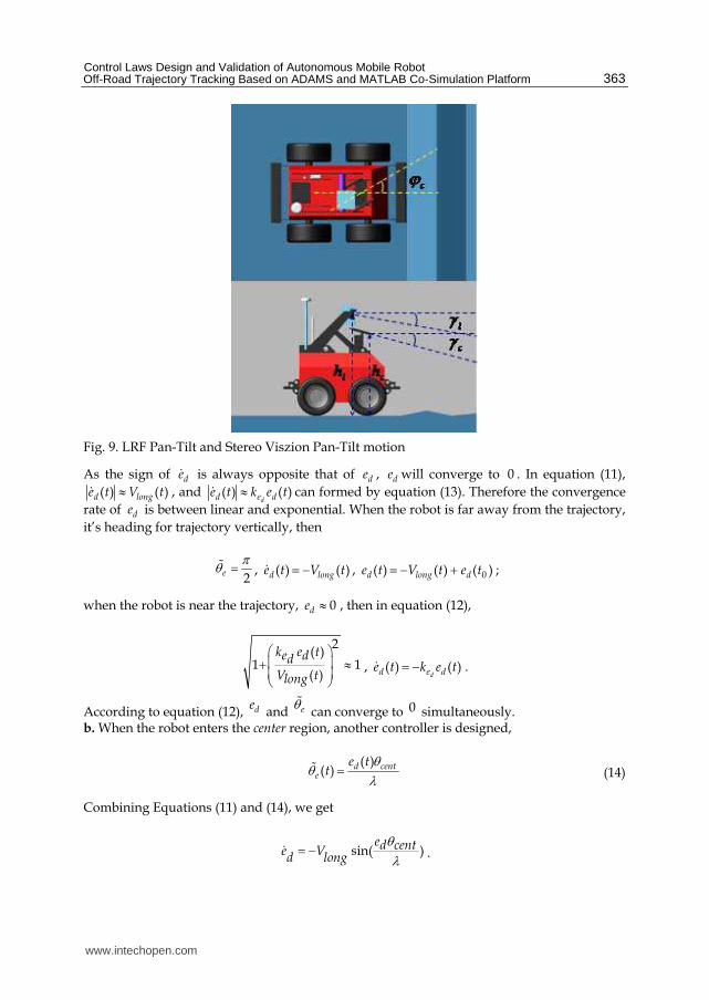
Fig. 9. LRF Pan-Tilt and Stereo Viszion Pan-Tilt motion

As the sign of de is always opposite that of de , de will converge to 0 . In equation (11),

( ) ( )d longe t V t , and ( ) ( )dd e de t k e t can formed by equation (13). Therefore the convergence

rate of de is between linear and exponential. When the robot is far away from the trajectory,

it’s heading for trajectory vertically, then

2

e

, ( ) ( )d longe t V t , 0( ) ( ) ( )d long de t V t e t ;

when the robot is near the trajectory, 0de , then in equation (12),

2( )

1 1( )

k e te ddV tlong

, ( ) ( )dd e de t k e t .

According to equation (12), de and e can converge to 0 simultaneously.

b. When the robot enters the center region, another controller is designed,

( )

( ) d cente

e tt

(14)

Combining Equations (11) and (14), we get

sin( )ed cente V

d long .

www.intechopen.com


364

In this region, de is very small, and consequently, ed cent

will also be very small, and then

sin( )e ed cent d cent

is derived. Therefore,

long

Ve long centd cente V ed d

, and then ( ) ( )exp{ }

1

Vlong cente t e td d

,

where 1t is the time when the robot enters the center region. In other word, de converges to

0 exponentially. Then, according to

( )ed centt

e , ( )e t converges to 0 .

So the origin is the only equilibrium in the ,d ee phase space.

3.3 LRF Pan-tilt and stereo vision pan-tilt control Perception is the key to high-speed off-road driving. A vehicle needs to have maximum data coverage on regions in its trajectory, but must also sense these regions in time to react to obstacles in its path. In off-road conditions, the vehicle is not guaranteed a traversable path through the environment, thus better sensor coverage provides improved safety when traveling. Therefore, it is important for off-road driving to apply active sensing technology. In the chapter, the angular control of the sensor pan-tilts assisted in achieving the active sensing of the robot. Equation (15) represents the relation between the angles measured, i.e.

c , c and l , of the sensors mounted on the robot and the motion state, i.e. e and x , of

the robot.

0 0

0 0

0 0

c c e

c c

l c

k

k x

k x

(15)

In (15), c , c are the pan angle and tilt angle of the stereo vision respectively. l is the tilt

angle of the LRF; ck , ck and lk are the experimental coefficients between the angles

measured and the motion state, and they are given by practical experiments of the sensors

and connected with the measurement range requirement of off-road driving. At the same

time, the coordinates of the scanning center are cot cosec c c c cx x h ,

cot sinec c c c cy y h ; and cotel l l lx x h , 0ely . In the above equations, cx , cy , lx ,

ly , respectively, are the coordinates of the sense center points of the stereo vision and LRF

in in-vehicle frame. As shown in Fig. 9, ch and lh are their height value, to the ground,

accordingly.

The angular control and the longitudinal control are achieved by PI controllers, and they are the same as the reference (Gabriel, 2007).

www.intechopen.com


365

4. Simulation tests

4.1 Simulation platform build In this section, ADAMS and MATLAB co-simulation platform is built up. In the course of

co-simulation, the platform can harmonize the control system and simulation machine

system, provide the 3D performance result, and record the experimental data. Based on the

analysis of the simulation result, the design of experiments in real world can become more

reasonable and safer.

First, based on the character data of the test agent, ATRV2, such as the geometrical

dimensions ( 65 105 80 )HLW cm , the mass value (118 )Kg , the diameter of the tire

( 38 )cm and so on, the simulated robot vehicle model is accomplished, as shown in Fig.10.

Fig. 10. ATRV2 and its model in ADAMS

Second, according to the test data of the tires of ATRV2, the attribute of the tires and the connection character between the tires and the ground are set. The ADAMS sensor interface module can be used to define the motion state sensors parameters, which can provide the information of position and orientation to ATRV2. It is road roughness that affects the dynamic performance of vehicles, the state of driving and the dynamic load of road. Therefore, the abilities of overcoming the stochastic road roughness of vehicles are the key to test the performance of the control law during off-road driving. In the paper, the simulation terrain model is built up by Gaussian-distributed pseudo random number sequence and power spectral density function (Ren, 2005). The details are described as follows:

a. Gaussian-distributed random number sequence ( )x t , whose variance 18 and mean

2.5E , is yielded;

b. The power spectral ( )XS f of ( )x t is worked out by Fourier transform of ( )XR , which

is the autocorrelation function of ,

2

2

2

( ) ( )

sin

j fX XS f R e d

fTT

fT

(16)

where T is the time interval of the pseudo random number sequence; c. Assume the following,

www.intechopen.com


366

+

( ) ( ) ( )= ( ) ( )y t x t h t x h t d (17)

2( ) ( ) j fth t H f e df (18)

where ( )h t is educed by inverse Fourier transform from ( )H f , and they both are real

even functions, then,

( )

( )( )

Y

X

S fH f

S f (19)

( )

( ) ( )

k

M M

r k rM M

y y kT

T x rT h kT rT T x h

(20)

where ( )YS f is the power spectral of ( )y t , ky is the pseudo random sequence of

( )YS f , 0, 1, 2 ,k N , and M can be established by the equation

lim ( ) 0mm M

h h MT ; d. Assign a certain value to the road roughness and adjust the parameters of the special

points on the road according to the test design, and the simulation test ground is shown in Fig. 11.

Fig. 11. The simulation test ground in ADAMS

4.2 Simulation tests In this section, the control law is validated with the ADAMS&MATLAB co-simulation platform.

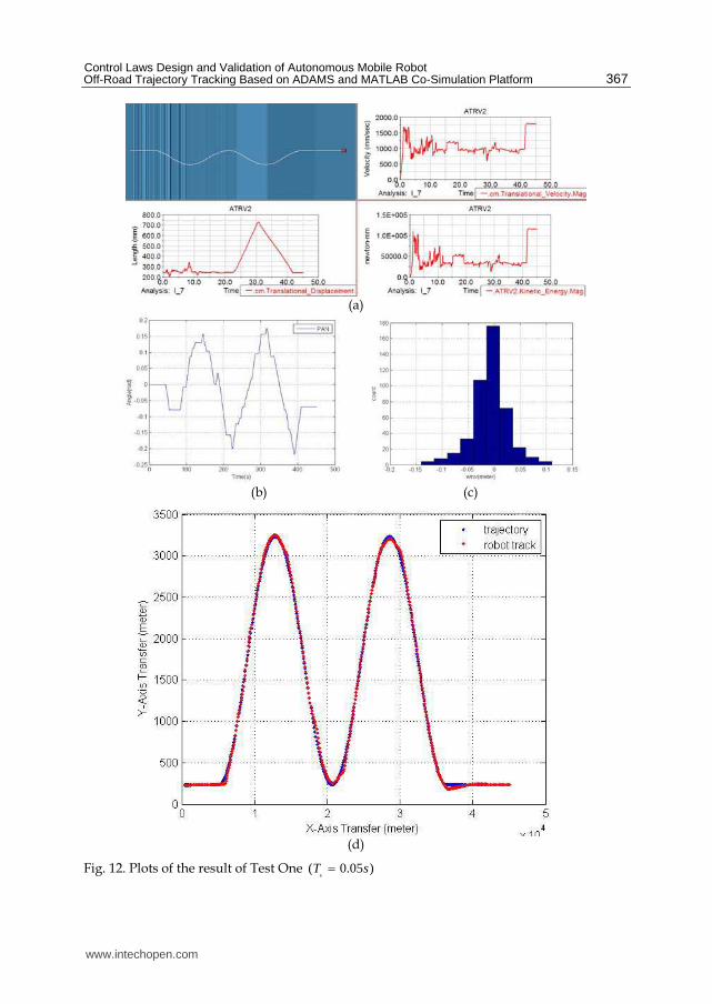
Based on the position-orientation information provided by the simulation sensors and the control law, the lateral, longitudinal motion of the robot and the sensors pan-tilts motion are achieved. The test is designed to make the robot track two different kinds of trajectories, including the straight line path, sinusoidal path and circle path. In Test One, the tracking trajectory consists of the straight line path and sinusoidal path, in which the wavelength of the sinusoidal path is 5 m , the amplitude is 3m . The simulation result of Test One is shown in Fig. 12. In Test Two, the tracking trajectory contains the straight line path and circle path, in which the radius of the circle path is 5m . The simulation result of Test Two is shown in Fig. 13.

www.intechopen.com


367

(a)

(b) (c)

(d)

Fig. 12. Plots of the result of Test One ( 0.05 )s

T s

www.intechopen.com


368

(a)

(b) (c)

(d)

Fig. 13. Plots of the result of Test Two ( 0.05 )s

T s

www.intechopen.com


369

In Fig. 12, which is the same as Fig. 13, sub-figure a is the simulation data recorded by ADAMS. In sub-figure a, the upper-left part is the 3D animation figure of the robot off-road driving on the simulation platform, in which the white path shows the motion trajectory of the robot. The upper-right part is the velocity magnitude figure of the robot. It is indicated that the velocity of the robot is adjusted according to the longitudinal control law. In addition, it is clear that the longitudinal control law, whose changes are mainly due to the curvature radius of the path and the road roughness, can assist the lateral control law to track the trajectory more accurately. In Test One, the average velocity approximately is 1.2 /m s , and in Test Two, the average velocity approximately is 1.0 /m s . The bottom-left part presents the height of the robot’s mass center during the robot’s tracking; in the figure, the road roughness can be implied. The bottom-right part shows that the kinetic energy magnitude is required by the robot motion in the course of tracking. In Sub-figure b, the angle data of the stereo vision pan rotation is indicated. The pan rotation angle varies according to the trajectory. Sub-figure c is the error statistic figure of trajectory tracking. As is shown, the error values almost converge to 0 . The factors, which produce these errors, include the roughness and the curvature variation of the trajectory. In Fig. 13 (d), the biggest error is yielded at the start point due to the start error between the start point and the trajectory. Sub-figure d is the trajectory tracking figure, which contains the objective trajectory and real tracking trajectory. It is obvious that the robot is able to recover from large disturbances, without intervention, and accomplish the tracking accurately.

5. Conclusions

The ADAMS&MATLAB co-simulation platform facilitates control method design, and dynamics modeling and analysis of the robot on the rough terrain. According to the practical requirement, the various terrain roughness and obstacles can be configured with modifying the relevant parameters of the simulation platform. In the simulation environment, the extensive experiments of control methods of rough terrain trajectory tracking of mobile robot can be achieved. The experiment results indicate that the control methods are robust and effective for the mobile robot running on the rough terrain. In addition, the simulation platform makes the experiment results more vivid and credible.

6. References

D. Lhomme-Desages, Ch. Grand, J-C. Guinot, “Model-based Control of a fast Rover over

natural Terrain,” Published in the Proceedings of CLAWAR’06: Int. Conf. on

Climbing and Walking Robots, Sept 2006.

Edward Tunstel, Ayanna Howard, Homayoun Seraji, “Fuzzy Rule-Based Reasoning for

Rover Safety and Survivability,” Proceedings of the 2001 IEEE International

Conference on Robotics & Automation, pp. 1413-1420, Seoul, Korea � May 21-26,

2001.

Gabriel M. Hoffmann, Claire J. Tomlin, Michael Montemerlo, and Sebastian Thrun (2007).

Autonomous Automobile Trajectory Tracking for Off-Road Driving: Controller

Design, Experimental Validation and Racing. Proceedings of the 2007 American

Control Conference, 2296-2301. New York City, USA.

www.intechopen.com


370

Gao Feng, “A Survey on Analysis and Design of Model-Based Fuzzy Control Systems,”

IEEE Transactions on Fuzzy Systems, Vol. 14, No. 5, pp. 676-697, 2006.

Gianluca Antonell, Stefano Chiaverini, and Giuseppe Fusco. “A Fuzzy-Logic-Based

Approach for Mobile Robot Path Tracking,” IEEE Transactions on Fuzzy Systems,

Vol. 15, No. 2, pp. 211-221, 2007.

José E. Naranjo, Carlos González, Ricardo García, and Teresa de Pedro, “Using Fuzzy Logic

in Automated Vehicle Control. IEEE Intelligent Systems,” Vol. 22, No. 1, pp. 36-45,

2007.

J.T. Economou, R.E. Colyer, “Modelling of Skid Steering and Fuzzy Logic Vehicle Ground

Interaction,” Proceedings of the American Control Conference, pp. 100-104,

Chicago, Illinois June 2000.

J. Y. Wong, “Theory of Ground Vehicles,” John Wiley and Sons, New York, USA, 1978.

Luca Caracciolo, Alessandro De Luca, and Stefano Iannitti, “Trajectory Tracking Control of a

Four-Wheel Differentially Driven Mobile Robot,” Proceedings of the 1999 IEEE

International Conference on Robotics & Automation, pp. 2632-2638. Detroit,

Michigan, USA.

Matthew Spenko, Yoji Kuroda,Steven Dubowsky, and Karl Iagnemma, “Hazard avoidance

for High-Speed Mobile Robots in Rough Terrain”, Journal of Field Robotics, Vol. 23,

No. 5, pp. 311–331, 2006.

Ren Weiqun. Virtual Prototype in Vehicle-Road Dynamics System, Chapter Four. Publishing

House of Electronics Industry, Beijing, China.

www.intechopen.com

Applications of MATLAB in Science and EngineeringEdited by Prof. Tadeusz Michalowski

ISBN 978-953-307-708-6Hard cover, 510 pagesPublisher InTechPublished online 09, September, 2011Published in print edition September, 2011

InTech EuropeUniversity Campus STeP Ri Slavka Krautzeka 83/A 51000 Rijeka, Croatia Phone: +385 (51) 770 447 Fax: +385 (51) 686 166www.intechopen.com

InTech ChinaUnit 405, Office Block, Hotel Equatorial Shanghai No.65, Yan An Road (West), Shanghai, 200040, China

Phone: +86-21-62489820 Fax: +86-21-62489821

The book consists of 24 chapters illustrating a wide range of areas where MATLAB tools are applied. Theseareas include mathematics, physics, chemistry and chemical engineering, mechanical engineering, biological(molecular biology) and medical sciences, communication and control systems, digital signal, image and videoprocessing, system modeling and simulation. Many interesting problems have been included throughout thebook, and its contents will be beneficial for students and professionals in wide areas of interest.

How to referenceIn order to correctly reference this scholarly work, feel free to copy and paste the following:

Yang. Yi, Fu. Mengyin, Zhu. Hao and Xiong. Guangming (2011). Control Laws Design and Validation ofAutonomous Mobile Robot Off-Road Trajectory Tracking Based on ADAMS and MATLAB Co-SimulationPlatform, Applications of MATLAB in Science and Engineering, Prof. Tadeusz Michalowski (Ed.), ISBN: 978-953-307-708-6, InTech, Available from: http://www.intechopen.com/books/applications-of-matlab-in-science-and-engineering/control-laws-design-and-validation-of-autonomous-mobile-robot-off-road-trajectory-tracking-based-on-

© 2011 The Author(s). Licensee IntechOpen. This chapter is distributedunder the terms of the Creative Commons Attribution-NonCommercial-ShareAlike-3.0 License, which permits use, distribution and reproduction fornon-commercial purposes, provided the original is properly cited andderivative works building on this content are distributed under the samelicense.

https://creativecommons.org/licenses/by-nc-sa/3.0/

control laws design and validation of autonomous mobile

Documents