control methodologies for relative motion reproduction...

Control Methodologies for Relative Motion

Reproduction in a Robotic Hybrid Test Simulation of

Aerial Refuelling

Jonathan Luke du Bois∗, Peter Thomas†, Steve Bullock‡,

Ujjar Bhandari§ and Thomas S. Richardson¶

Aerospace Engineering Department, University of Bristol, Bristol BS8 1TR

In many applications it is advantageous to simulate the relative motion of two bodies

in a laboratory environment. This permits the testing of sensors and systems critical

to the safety of equipment and personnel with reduced risk, and facilitates stage-gate

management of large projects to mitigate financial risks. The University of Bristol is

collaborating with Cobham Mission Equipment to develop a large-scale facility for relative

motion simulation, primarily for the purpose of testing automated air-to-air refuelling

systems. The facility incorporates two 6DOF articulated robotic arms whose motion is

dictated by real-time numerical simulations of the physical environment. Sensors on the

robot-mounted equipment feed back into the numerical simulation to perform closed loop

simulations with real hardware. This paper discusses the development of the facility and the

different approaches considered for achieving real-time control of the robotic hardware. It

then goes on to focus on aspects of the control topologies and motion optimisation which are

used to maximise the performance of the facility. The current capabilities are demonstrated

with respect to an aerial refuelling exercise and future challenges are explored.

I. Introduction

As computational processing power and, significantly, actuation technologies improve, an increasinglypopular technique is that of Hybrid Testing. Hybrid tests involve the testing of physical subassemblies in areal-time simulation, coupled to numerical simulations of complete systems and their related environmentalconditions. Sometimes referred to as real time dynamic substructuring, or likened to hardware-in-the-loop(HiL) testing, they promise the ability to test the performance of components in a highly realistic operatingenvironment while remaining within the low-cost, repeatable, and relatively safe confines of a laboratory.

This paper describes steps in the development of a hybrid testing facility specifically targetting applica-tions involving relative motion between two independent bodies. Often this work will be related to sensingrequirements, with no direct contact between the two bodies. A prominent example is the case of satelitedocking approach, and it is unsurprising that some of the first large scale relative motion hybrid testingexperiments have been focused on this problem.1,2 The application examined here is that of to air-to-airrefuelling, where the system dynamics tend to have shorter timescales than those intended in satellite ma-noeuvers, and the relative motion is more erratic due to the unpredictable effects of atmospheric turbulence.

Air-to-air refuelling (AAR) was first conducted in experiments of the 1920s and has since evolved into anestablished means for extending the range, payload and endurance of manned aircraft.3 While its adoption incivil aviation sectors has been slow to emerge, there are numerous potential benefits, including the reductionof fuel consumption in passenger and freight transport, the reduction of airport loading, the extension ofrange and payload in existing aircraft, and increased scope for scientific and environmental surveys throughimproved endurance.

∗Research Associate, Aerospace Engineering Department, University of Bristol†Research Assistant, Aerospace Engineering Department, University of Bristol‡Ph.D. Student, Aerospace Engineering Department, University of Bristol§Ph.D. Student, Aerospace Engineering Department, University of Bristol¶Senior Lecturer, Aerospace Engineering Department, University of Bristol

1 of 21

American Institute of Aeronautics and Astronautics

AIAA Guidance, Navigation, and Control Conference13 - 16 August 2012, Minneapolis, Minnesota

AIAA 2012-4676

Copyright © 2012 by the University of Bristol. Published by the American Institute of Aeronautics and Astronautics, Inc., with permission.

Two popular methods have arisen for AAR: the Flying Boom developed by Boeing,4 and the probe anddrogue method pioneered by Flight Refuelling Ltd.5 (now Cobham). In the former, a retractable boom isextended from the tanker aircraft, and steered by means of two “ruddervators”, aerodynamic control surfacesattached to the boom. An operator in the tanker aircraft steers the tip of the boom to a coupling on thereceiver aircraft, which holds a formation position below and to the aft of the tanker. For probe and droguerefuelling the tanker trails a flexible hose terminating in a drogue assembly, comprised of a canopy to providestability and a coupling for the fuel transfer. The receiver aircraft is equipped with a probe, rigidly mountedto the aircraft, which is manouevered into the drogue by the pilot. In this mode of AAR the receiver aircraftmust be agile enough to steer the probe into the passive drogue.

In unmanned aerial vehicles (UAVs), where endurance is no longer limited by pilot fatigue, aerial refuellingcapabilities offer significant benefits. Refuelling operations have historically been conducted as a pilotedoperation demanding a high level of training and fast reactions, and as such can not be conducted forremotely piloted aircraft over slow data links. The recent proliferation of UAVs has therefore resulted in ademand for automated air-to-air refuelling (AAAR) capabilities and it is this requirement that motivatesthe development of the test facilities described in this paper. Successful accomplishment of AAAR relies onthe development of two key technologies: firstly, position sensing and tracking, to allow a boom to determinethe relative position of the receiver’s fuel coupling or a receiver aircraft to determine the relative positon ofthe refuelling drogue; and secondly, control strategies, to enable robust and safe operation of the boom andthe receiver aircraft in steering them to their target.

There have been extensive works on appropriate control systems developed with numerical flight simu-lations, using for example traditional PID and LQR methods, gain scheduling,6,7 adaptive controllers suchas neural networks8,9 and model reference adaptive control,10 differential game approaches,11–13 and feed-back linearisation techniques.14 Other work has investigated fault tolerance15 and actuator failure cases.16

Numerical simulations have been enhanced with the inclusion of turbulence models and the development ofimproved tanker wake models17 and drogue modelling.18 In addition to the simulation results of the abovestudies, actual flight tests have been successfully conducted demonstrating formation flying and movingbetween stations for both the boom19,20 and the probe and drogue21–23 methods. The latter study alsodemonstrated full contact with the drogue on one flight, engaging successfully on two out of six attempts.

For postition tracking in AAAR, a variety of sensing technologies have been employed, including inertialmeasurements,24 differential GPS (DGPS) and electo-optical systems. Often these are employed in tandemusing wireless telemetry25 and sensor fusion methods: Williamson et al.,25 for example, used Kalman Filteringin their laboratory-based flying boom experiments. Similarly, the combination of GPS measurements withposition estimates from vision systems has been explored in a number of publications,26–31 where the principalapproach is to use the GPS measurements predominantly at a distance, filtering in the machine vision datawith increasing proximity to the target. Junkins et al. developed a novel low-power optical system calledVisNav32 which has been used in several AAAR studies.33–36 Also advocating the use of beacons, Pollini et

al.37,38 proposed placing light emitting diodes (LEDs) on the drogue and using an inexpensive CCD webcamwith an infra-red filter to identify the LEDs.

The development of these two technologies relies on sophisticated testing: the sensor development requiresphysical tests under realistic conditions, while the control algorithm development leans heavily on realisticsensor data to ensure robust operation. The work described here is concerned with creating a laboratorytest facility that can satisfy these requirements, providing the most comprehensive evaluation possible forthese new aerial refuelling technologies prior to flight testing. The facility uses two industrial robotic armsto manipulate the refuelling hardware for the two aircraft, driven by a numerical simulation of the flightdynamics and structural and aerodynamic models. Robots have been used in previous papers to simulateaircraft motion in refuelling operations, for example Pollini et al.38 used a robot to recreate aircraft motionto test vision system algorithms, but the aircraft control loop was not closed. In the setup described in thispaper the sensors feed directly back into the numerical simulation of the flight dynamics, providing realistictests in a controlled environment.

The robotic cell is comprised of two 6 degree-of-freedom (6DOF) robot arms, one of which is mounted ona linear track. Full scale refuelling hardware is mounted on the robots, and a large range of relative motioncan be accomodated to simulate the final 10m of the approach in an aerial refuelling procedure. The layoutof the robot cell is shown in Fig. 1 and a photograph illustrating the refuelling components can be seen inFig. 2.

Section II examines the problem of real time control of large scale robotic hardware using readily avail-

2 of 21


Figure 1. Plan view of robot cell, depicting aerial refuelling hardware and coordinate system.

Reception

coupling

Canopy

RibsR1

Mounting

plate

R2

Nozzle

Probe

Mounting

plate

Track

Figure 2. Photograph of robot cell, showing aerial refuelling hardware mounted on robots.

able commercial equipment, looking at three different control approaches and describing their merits anddrawbacks. Section III presents a high level interface approach and examines the achievable performance.Addressing shortcomings in this approach, Section IV describes preliminary tests of a low level interface andsets out important safety considerations for a facility of this scale. Section V discusses optimisation of themotion paths, looking at peculiarities of the physics of robot arm manipulators in this type of application.Section VI then presents the flight dynamics simulation for use in the aerial refuelling tasks and showsthe preliminary performance results for the facility. Conclusions are drawn and future work is discussed inSection VII.

II. Control Topologies

The robots used in the Bristol University relative motion robotic facility are ABB IRB6640 production-linerobots and are supplied with a proprietary IRC5 controller. The robots are electromechanically driven andeach has 6 joints capable of producing 6DOF motion in three Cartesian coordinates and three orientationalaxes, with accelerations up to 2g and velocities of more than 2m/s. The IRC5 controller provides a highlevel of functionality, including coordinate transformations, kinematic computations and motor control loopswhich take account of the robot geometry, inertia and payload information. Importantly, the proprietarycontroller also provides several layers of safety controls to protect operators and equipment.

In normal operation, the user would program the robots using a high-level language called RAPID code.

3 of 21


The instructions used in the RAPID code provide a powerful tool for quickly generating complex motionpaths and creating loops and conditional operation patterns. The language facilitates a variety of inputand output (I/O) methods, including analogue and digital I/O channels as well as ethernet communicationprotocols. The data sent and received on these channels can be used in the RAPID code to affect theoperation of the robots.

In robot operation, the RAPID interpreter executes motion instructions which pass the motion commandsto a motion planning routine. This planning routine performs kinematic computations and sends the jointmotor demands to the axis computer. As well as accepting position demands, the robots are capable ofoperating in force control mode, using 6DOF force and torque sensors mounted at the end effectors. In thiscase a nominal motion is specified as well as force demands, and deviations of the measured force from theforce demand affect the motion path accordingly.

Three approaches are considered here for the implementation of the closed-loop hybrid tests:

• high level (through RAPID)

• mid level (exploiting force control inputs and using auxiliary feedback)

• low level (direct access to axis computer of robot controller)

The biggest advantage of the first two options is that they retain the robust safety mechanisms of theproprietary controller, and thus permit faster development of auxiliary control without the fear of seriousmalfunction and injury or damage. The high level option also retains the matured control technology ofthe proprietary controller, providing the best motion path control for the least development effort. This isprovided at the cost of deterministic real-time control; the RAPID code is not intended to receive, parseand compute small motion path segmenets on the fly in this manner. Methods to provide determinismare discussed in Section III, but these introduce delays in the robot motion with respect to the numericalsimulation.

The mid level control option uses the input signals normally used for force control feedback to affect themotion of the robots. In this manner the RAPID interpreter and much of the motion planning algorithmis bypassed, resulting in a much faster control loop. The safety of the proprietary controller is preserved,as are the kinematic computations and coordinate transformations; thus the auxilliary control can still beapplied in the Cartesian coordinate space. The voltage signals provided at the force control interface produceproportional velocities in the robot motion. There is no interface available at this level for positional feedback,so for closed loop position control it is necessary to take advantage of auxiliary sensors. A specific drawback ofthis method is that the new feedback control must be tuned and will not easily achieve the same performanceas the inner loop proprietary control.

The third and final option is to directly access the axis computer of the robot controller. This methodeffectively bypasses all of the proprietary control systems and sends demands directly to the position feedbackcontroller for the robot motors. Whilst offering the best control of the robots, adopting this approach requiresby far the largest development effort, and forsakes much of the intrinsic accuracy of the industrial controller.A further consideration is that this technique will undermine some of the more sophisticated elements of thesafety controller, and alternative safeguards must be implemented.

III. Determinism in a High-Level Approach

In this section the high-level approach is considered in detail. The biggest barrier to implementing areal time scheme using this approach lies in the non-determinism of the communication protocols and theunpredictable nature of the RAPID code interpretation. The former is imposed by the implementation ofTCP/IP ethernet communications on the robot controller. The unpredictable nature of the RAPID codeis due to the fact that it is being interpreted on a processor running a variety of concurrent threads soexecution can slow down when the processor is heavily loaded. In normal operation this is not perceptiblebut when positions are being demanded at rates of 10Hz or more the system is sensitive to small delays inthe execution cycle. Methods for mitigating these effects and providing a real time deterministic motionbased on the deterministic outputs of the numerical simulation are described below.

The flow of position information from the flight dynamics model (FDM) simulations to the actual robotmotion is illustrated in Figure 3. Three physical devices are depicted (where the robots and the track areincluded as a single system for these purposes). The most important elements in the discussion that follows

4 of 21


are the PXIe real-time controller and the IRC5 robot controller. The communication between these elementsis by means of ethernet TCP/IP streams, carried over 100BASE-TX using a Category 5 crossover cable.

The FDM simulation is shown in the bottom right corner; the complexity of this system is belied by itsrepresentation on this diagram but is elaborated in Section VI. The simulation runs at 1 kHz on the realtime Veristand Engine operating system of the PXIe box. This operating system is capable of overseeing thedeterministic execution of multiple models, or processes at defined rates. The primary control loop executesthe FDM model and the supervisory process in turn, both at a rate of 1 kHz. At the start of each time stepfor a given process the data mappings into that process are read from the buffers, and when it executes,the outputs of the process are written to the buffers. The data mappings between processes are referredto as channels, and this is how information is exchanged between the processes on the PXIe. Critically, nodata can be exchanged mid-way through a time step of a particular process. Note that the processes canbe configured to run in parallel or consecutively, and in the latter case the outputs of earlier processes willbe available for later processes within the same time step. In the current application the FDM is the firstprocess to run each time step, and the position data from the FDM is made available to the supervisorprocess. This data is passed as 64-bit double precision floating point variables.

The supervisory process performs many tasks, including providing execution control for the FDM, butits most critical task is to control the flow of data to and from the ABB IRC5 controller. The key technicalbarrier is that while the FDM and supervisory process are both run in real time, and the robot motion can becontrolled such that it meets position demands in deterministic time frames, the communication protocolsdo not mirror this determinism. On the IRC5 side of the communications, the data transmission bufferand process/thread management is handled internally by proprietary firmware and very limited control canbe exercised over these processes. On the PXIe side of the communications, the so-called custom device

process responsible for the TCP/IP transmissions necessarily runs asynchronously with respect to the realtime processes to avoid delaying any time steps in the event of a delayed message from the IRC5 controller.The design of the custom device will be described presently. The supervisory process controls the flow ofdata to and from the IRC5 controller using two sets of counters: the first set is used to synchronise with thecycles of the IRC5 communication loops and will be discussed shortly with reference to the TCP/IP customdevice. The second set of counters are the COMM and ACKN indices seen in Figure 3. These are usedto orchestrate the motion commands sent to the IRC5. The position demands from the FDM are sampledregularly at 20Hz using a timing pulse trigger to ensure a smooth motion path definition. These are thenplaced into a FIFO buffer so that no position data will be omitted in the event of communication delays.Each position dataset is sent to the IRC5 with a unique, sequential COMM (command) index. Once theposition instruction has been completed on the IRC5 it returns the corresponding ACKN (acknowledge)index. The receipt of this index by the supervisory process provides the ACKN trigger used to send the nextbuffer entry. In general operation this buffer remains empty, with the position instructions being removedfrom the buffer in the same time-step that they are placed in it. It is nonetheless a necessary feature toprevent errors in the event of communication speed fluctuations.

The TCP/IP communications process on the PXIe is implemented as a custom device in the VeristandEngine, running asynchronously with respect to the real time processes, interfacing with the IRC5 controlleron one side via a TCP/IP socket and with the real-time supervisory process on the other side by means of64-bit floating point data channels, read from and written to FIFO buffers in the shared memory space at thestart and end of each custom device loop. Data received from the IRC5 includes measured positions derivedfrom the joint encoders, timing data used in the supervisor process to optimise position sampling timing,timestamps for measured data, and control variables such as the ACKN index and cycle synchronisationcounter. Data sent to the IRC5 includes the position demands from the supervisory process, the COMMindex, the cycle synchronisation counter and the sampling time (currently held constant at 0.05 s↔20Hz). The communications run faster than the 20 Hz position demands, to permit measurements to berecorded at a higher frequency. The custom device runs asynchronously, using the COMM/ACKN indicesto trigger the motion instruction events. The second set of counters, used to synchronise with the IRC5cycle and referred to as IRC5iteration and PXIiteration, ensure that the communications to and fro alwaysinterleave the processing loops. That is, the supervisory loop will always run once following the receipt ofa message from the IRC5 before a message is sent back to the IRC5, and vice versa for the motion controland measurement loop on the IRC5. This involves repeatedly looping following receipt of a TCP messageuntil PXIiteration=IRC5iteration, indicating the supervisory process has processed the received data, andonly then sending a message back to the IRC5. Messages from the IRC5 controller are comprised of ASCII

5 of 21


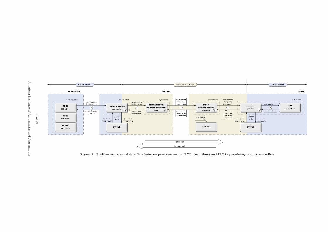
Figure 3. Position and control data flow between processes on the PXIe (real time) and IRC5 (proprietary robot) controllers

6of21

Am

erican

Institu

teofA

eronautics

and

Astro

nautics

string representations of the numerical values, separated by commas and terminated by a CRLF(0D0A)sequence. This is a legacy system and will be replaced in due course, but the performance analysis presentedbelow illustrates that it does not impose a severe performance penalty. It does impact on the precision ofthe data transmissions, but this does not have a real effect on the accuracy of the position demands andmeasurements. In contrast, the string parsing functions on the IRC5 are not well suited to processing longstrings of numerical values and in this direction the values are now encoded as 32-bit floats, with big-endianbit ordering and little-endian byte ordering, in a fixed-length message with start delimiting header bytes.These can be efficiently reconstructed at the IRC5 end. The secondary responsibility of the custom deviceis for the logging of all data sent in each direction. This will include all available measured values as well asperformance and timing data, and demanded positions.

On the IRC5, the equivalent of the PXIe’s supervisor process is the motion planning and control process.This process is handled by proprietary ABB firmware, and currently the only means of influencing the processis to issue move instructions from a high-level scripting code called RAPID. When a move instruction is issued,the motion planning process buffers the position data and once the buffer contains sufficient positions itconstructs a smooth path, interpolating at the corners. The move instruction contains position data as wellas a time-step indicating the time the robot should take to complete the motion from the previous point tothe new point. Provided the buffer is replenished at the same rate the motions are completed, the plannedpath is iteratively updated to ensure a continuous motion. This buffering process introduces a delay betweenthe FDM simulation and the robot motion (augmented to a small extent by the transmission times, messageprocessing, and position filtering), and this delay must be compensated for as described below.

The RAPID script loop which serves as the gateway to the IRC5 controller, mirroring the TCP/IP customdevice on the PXIe, is independent of the motion planning, and needs only to supply motion instructionsas they are made available over the communications link. It performs a simple loop, repeatedly measuringpositions, recording timing information, sending these to the PXIe along with the ACKNindex and PXIiter-ation counters, and awaiting a response from the PXIe. Once a response is received, if the COMMindex hasincremented then a move instruction is executed and the ACKNindex is adjusted. The loop then repeats.

The measurement data from the IRC5 can be received at rates of around 100Hz under favourable con-ditions, but the timing of the measurements is not regular and they can be interrupted by the motionplanning routines, which run with a higher priority. In addition, the measurements thus obtained make theassumptions of zero backlash, accurate geometry models, and most importantly no structural flexibility.

This section now concludes with an analysis of the timing of the communications cycles. Firstly, Figure 4shows the current case of a 20 Hz motion path update. The stacked bars indicate the times that the respectivetasks have taken on the IRC5 controller for each time step. The total height of each bar is proportional toits width, and represents the time for a full cycle to complete. The precision of the measurements is 1 ms,which in some cases is too small to measure a time difference in some of the execution steps. The cycles aredivided into six stages: the messageCompose stage is where the measurement and timestamp data is aquiredand sequenced into a message ready for transmission from the IRC5 controller; the messageSend stage iswhere this message is sent over the TCP/IP link; the messageReceive stage is where the position demandand control data are received over the TCP/IP link; the messageParse stage is where the received message istranscribed into the appropriate variables on the controller; the moveInstruction stage is where the motioncommand is issued to the motion planning routines in the IRC5 controller, and finally the cycleTime stageis simply the time for the cycle to return to the beginning of the loop. The latter stage takes negligible timebut sometimes appears as a millisecond in the figures presented as an artefact of rounding errors.

In the case presented in Figure 4, the communication loop was locked to the main cycle. That is, theonly time the PXIe was sending messages to the IRC5 was when a motion command needed to be sent.Accordingly, every cycle takes approximately 50 ms, corresponding to a 20 Hz cycle rate. It is by chancethat the bottleneck in the case presented is waiting for the latest sample to be buffered from the FDMsimulation by the supervisory process. That is why the IRC5 time data indicates a large proportion of thecycle time is spent waiting to receive a message from the PXIe. If the time was not allocated here, it wouldbe spent waiting to buffer the position data when the move instruction was executed in the IRC5. It can beseen that the composition of the message string to send takes a comparable time to that taken to read thebinary message received from the PXIe.

Figure 5 shows an earlier test performed at 10 Hz. In this case, however, the communication cycleis not locked to the position instruction cycle, and intermediate communications relay measurements tothe PXIe. In this case a standard communication cycle takes around 10 ms. The cycles where a move

7 of 21


133.4 133.6 133.8 134 134.2 134.4 134.6 134.8 1350

10

20

30

40

50

60

time (s)tim

e (m

s)

cycleTimemoveInstructionmessageParsemessageReceivemessageSendmessageCompose

Figure 4. Stacked bar chart depicting breakdown of the times for the tasks in each communication cycle on the IRC5controller. This data is for a 20 Hz motion rate. The precision of the time measurements is 1 ms. (Case 1)

15.8 15.9 16 16.1 16.2 16.3 16.4 16.5 16.6 16.7 16.80

2

4

6

8

10

12

14

16

18

20

time (s)

time

(ms)


Figure 5. Stacked bar chart depicting breakdown of the times for the tasks in each communication cycle on the IRC5controller. This data is for a 10 Hz motion rate, after changing to a binary communication protocol. The precision ofthe time measurements is 1 ms. (Case 2)

12 12.5 13 13.50

10

20

30

40

50

60

70

time (s)

time

(ms)


Figure 6. Stacked bar chart depicting breakdown of the times for the tasks in each communication cycle on the IRC5controller. This data is for a 10 Hz motion rate, using an ASCII communication protocol, prior to changing to a binarycommunication protocol. The precision of the time measurements is 1 ms. (Case 3)

8 of 21


instruction is received at the IRC5 can be seen, as the cycle takes longer, with the time taken to processthe move instruction accounting for the difference. These cycles are spaced at approximately 0.1 s intervalsas expected, and the time spent processing the move command is the time needed to regulate the motiontiming at the IRC5 end.

Finally, Figure 6 shows another example, but this time no position data is sent (i.e. the COMM indexremains at zero). In this case, however, the messages from the PXIe to the IRC5 are encoded as ASCIIstrings of numeric values, requiring string parsing on the IRC5. It can be seen here that the message parsingon the IRC5 takes around 30ms, far greater than the < 10 ms taken to decode an equivalent binary messagein Figure 4. In the final figure the receive stage of the cycle also takes around 30 ms. This was found to becaused by diagnostic console output being written to the screen on the PXIe, slowing down the cycle time.The average times for the six stages over the three cases are given in Table 1.

Also of interest is the behaviour of the IRC5 controller when it is first sent position demands. Fig. 7(a)shows the timing of the communication cycle tasks, with the position demands sent at a rate of 10Hz startingjust before 19s. When the position demands first commence, a small, 20ms spike can be seen correspondingto the move instruction for the first position demand. The second move instruction takes slightly morethan 100ms to process, and the third takes over 250ms, before settling down to a more regular pattern ofapproximately 100ms, corresponding to the 10Hz demand rate.

Fig. 7(b) shows the number of move instructions executed in the RAPID code compared to the numberof motions actually completed by the robots. It can be seen that the robot motion does not begin untilafter the move instruction times settle into this regular pattern. This delayed start, combined with theregulating effect of the 100ms move instruction times, ensures a delay of approximately 0.5s between theposition demand of the real time simulation and the motion of the robots. It was found that independentof the position demand rate, the robot controller always queued up approximately half a second’s worth ofmotion instructions before commencing the actual motion, resulting in an unavoidable 0.5s delay.

This level of delay is clearly unacceptable in a real-time control environment. Several options presentthemselves: the first is to apply compensation techniques, designed to cancel the dynamics of the roboticinterface hardware, including the delay. Previous studies in the context of structural-HiL-style testing haveshown that in continuous systems a reasonable compensation can be provided by a simple polynomial forwardpredictive capability.39–41 More advanced approaches are evaluated by Chen and Ricles42 in this context.All of these methods rely on predictions of future demand signals, however, and will deal badly with severenonlinearities and discontinuities. To address the problem fully, the performance of the equipment, includingthe controller, must be improved intrinsically. It is in this pursuit that low level control is now being pursedat the University of Bristol.

Table 1. Average times, in milliseconds, for the six stages of the communication and control loop on the IRC5 robotcontroller, for the three cases described in Figures 4-6.

Case 1 Case 2 Case 3

messageCompose 3.75 4.09 4.96

messageSend 0.53 0.21 0.04

messageReceive 37.78 2.23 25.14

messageParse 3.15 1.33 29.56

moveInstruction 4.78 0.56 0.2

cycleTime 0.08 0.1 0.24

9 of 21


(a) Stacked bar chart showing communication cycle timingas the PXIe begins sending position demands to the IRC5at a rate of 10Hz.

(b) Counters showing the number of motion instructionsprocessed in the RAPID code and the number of motionscompleted by the robots.

Figure 7. Timing data as motion commands are commenced.

IV. Safe Operation of a Low Level Approach

To facilitate low-level control of the robot hardware, the Open Robot Control Architecture (ORCA) ofthe University of Lund43 has been adopted. This control uses a separate ORCA PC which intercepts signalssent between the main computer and the axis computer in the IRC5 controller. It can then augment oroverride the signals sent to the axis computer and demand joint motor positions directly. Fig. 8 showssignals measured at the PXIe machine as a step input signal is sent to the IRC5 through the ORCA interfacein initial testing. The sample rate on the PXIe is 100Hz, in keeping with the primary control loop running theFDM. The reference input signal is sent from the PXIe to the IRC5 and is returned as the recorded referencesignal from the IRC5 within a single 10ms timestep. In the next 10ms timestep the robot is measured tohave initiated its motion. This is already a marked improvement on the > 500ms delay introduced in thehigh-level approach. In the timesteps that follow, the measured robot position is seen to follow a first-ordercharacteristic to approach the reference demand.

18 18.05 18.1 18.15 18.2

0

0.5

1

1.5

2

2.5

3

3.5

time (seconds)

mot

or a

ngle

(ra

dian

s)

PXIe refABB IRC5 refABB IRC5 measured

Figure 8. Signals measured at the PXIe (used to run the real-time simulations) in response to a step input sent to theIRC5 (robot controller) via the low level interface.

10 of 21


While the <20ms latency in initiation of motion is reasonable, the positional response needs to beimproved. A schematic layout of the axis computer control is shown in Fig. 9. In the preliminary testsdescribed, only a position input was used. To improve on the performance of the robots, ABB use velocityand torque feedforward demands as seen in the figure. The torque signals are considered commerciallysensitive, and are disabled by ABB as part of the licensing agreement for the ORCA interface, but thevelocity feedforward is still available for use through ORCA. In addition, the controller gains can also betuned through ORCA, allowing gain scheduling. In implementing these steps a much improved response isexpected. A torque feedforward could even be reinstated in a limited capacity by using an inverted controllerto cancel the effects of the PI controller in the torque feedforward signal.

Figure 9. Schematic showing the operation of the axis computer

A concern that remains is that by directly passing demands to the axis computer, the robust safety ofthe industrial control systems are bypassed to some extenta. To minimise the risk to equipment, and to avery limited extent to people, the approach adopted here is to use the ORCA interrface only to augment

the control of the robots. The high-level interface remains as the primary input to the robot control, withthe ORCA interface used to augment the position to compensate the delay in the high-level control. Theextent to which the ORCA interface can modify the signal from the IRC5 main computer is strictly limited,ensuring the robots do not deviate significantly from the safety-assured path determined by the main IRC5controller. The layout of this system is shown in Fig. 10.

Figure 10. Overview of the position control in the augemented low-level approach. Safety is assured by limitingdeviation from the path determined by the main IRC5 computer.

The approach presented is expected to produce fast system response times without forsaking the ro-bust safety of the high-level approach. Once this is achieved, some more practical considerations must beaddressed, and these are examined in the next section.

V. Motion Path Optimisation

Besides the work on minimising latencies described in the preceding sections, work is ongoing on opti-mising the motion paths of the two robots to maximise the performance envelope. The nature of the roboticarms means that they do not have constant performance within the workspace, and their capabilities are

aSpeed limits and absolute joint limits remain in place but more refined control of the operational limits are undermined bythe approach.

11 of 21


affected by the configuration of the joints in any given poisition. In particular, three types of singularityexist in the kinematic solution and as these are approached the achievable velocity approaches zero.

Fig. 11 shows preliminary data gathered in the course of an undergraduate research project, depicitingthe variation of horizontal velocity with position throughout a plane when commanded to move across theplane at maximum speed. The low velocities at the left and right of the graph indicate the accelerationand deceleration at the start and end of the motion. The low velocities in the central region are due tothe singularity. Note that the data above 1350mm in the Z axis is simply mirrored from that below, as thegraph was used for illustrative purposes. The performance of the robots can be characterised in this mannerthroughout the working volume, and the points of peak perfomance identified. These points are obviouschoices as the nominal resting position of the robots, but the interesting results arise when considering therelative motion of the two robots.

Figure 11. Speeds of the robot traversing a plane in lines along the y axis, starting and finishing at zero velocity atthe left and right sides of the figure. Data above 1350mm in the Z axis is mirrored from that below for illustrativepurposes. Source: undergraduate research project44

A performance index can be derived based on the maximum achievable speed and acceleration for a givenjoint configuration. For any specific relative displacement of the two robot end effectors, there is a continuousset of positions that satisfies the relative pose; the objective is to maximise the performance index at alltimes, subject to the constraints of actually following the demanded relative motion path.

The performance index would most likely be best evaluated through the use of a kinematic model dueto the order of the parameter space (6DOF→6th order parameter space). This model should be validatedexperimentally as in Fig. 11, but would then be used in isolation for the controller. The Jacobian of theperformance index would be used to augment the absolute motion of the two robots while maintaining thedemanded relative motion. Work on this topic has begun and will compliment the reductions in signallatencies described herein to optimise the overall performance of the facility.

VI. Flight Dynamics Simulations

In this final section, a simulation environment is presented to encompass the flight dynamics and refu-elling environment, and initial performance tests from the RMR are analysed. Simulations are written inMathworks’ Simulink environment and compiled with the Simulink Coder (Real Time Workshop) toolboxfor use on the PXIe platform using National Instruments’ Veristand target language compiler. Simulationscover the wider refuelling scenario in order to develop and investigate control strategies, with the RMRspecifically providing the HIL capability for the more complex hook-up space. The simulation environmenttakes into account:

1. Tanker trajectory demands and control, FCS and flight dynamics model.

2. Models of the hose and drogue assembly

3. Receiver navigation logic, FCS and flight dynamics model.

4. Atmospheric (gust and wake) disturbance models

12 of 21


The simulation structure is purposely modular such that ongoing improvements to individual componentscan be made in parallel and swapped in, limiting the changes needed to the simulation environment.

The purpose of the simulation, in the context of the RMR facility, is to generate position and orientationinformation for the probe and drogue which can be replicated by the manipulators. To that end we definea set of axes systems in Figure 12 which identifies the refuelling probe (p) and paradrogue (d) objects. Thetask in probe-drogue configured AAR is to approach and couple the probe with the drogue to close the refuelline. Consequently the probe must track and close the range between it and the drogue, this is describedin terms of the approach frame (a) which is coincident with the drogue. The probe position is thereforedescribed with the coordinates (xp, yp, zp), relative to the origin oa.

zp

xp

yp

yd

xd

zd

oa

θpψp

ϕp(xp, yp, zp)

axa

ya

za

Figure 12. Probe (p), drogue (d), and approach (a) axes definitions.

VI.A. Aircraft models

Both the receiver and tanker are rigid-body, six degrees of freedom objects having nonlinear aerodynamicbehaviour in the form of lookup data. The general schematic for the rigid bodies is illustrated in Figure13. Reference commands from the guidance and navigation systems are used by the flight control system togenerate input commands to the actuator models. These in turn, along with the dynamic aircraft states areused to generate the aerodynamic forces and moments on the aircraft at the centre of mass (CM). Clearly theCM will vary throughout the refuelling process, primarily affecting the pitching moment of both receiver andtanker. However up to now we have assumed the variation will have a negligible effect on the performance ofthe flight control laws and have used a fixed CM at 0.25c i.e. 25% from the leading edge of the wing’s meanaerodynamic chord. Future improvements to the simulation will determine if this was a valid assumption: ithas already been suggested that that mass variation due to fuel transfer compounds the difficulties createdby tanker wake turbulence.45 A generic tanker flight dynamics model is employed but the tanker dynamicsare not critical to the simulation - in simpler scenarios the tanker model has been replaced with a referencepoint moving at constant velocity. Two configurations for the receiver aircraft are used: an F-16 fighter jetand the conceptual Innovative Control Effector aircraft.

A model for an F-16 unmanned jet fighter was derived from the data in,46 which itself is a reduced versionfrom.47 The simplified model is valid for the aerodynamic range α ∈ [−10◦, 45◦], β ∈ [−30◦, 30◦], which iswell within the flight regime for refuelling aircraft. Three first order lags with rate limits and saturationsmodel the actuators similar to those used in.47 Aerodynamic forces and moment coefficients about the centreof mass (CM) are calculated in the aerodynamic subsystem using the previous time step aircraft states:

CX(α, q, δe) CY (α, β, p, r, δa, δr)

CZ(α, β, q, δe)

CL(α, β, p, r, δa, δr) CM (α, q, δe, CZ)

CN (α, β, p, r, δa, δr)

where α, β are the aerodynamic incidence and sideslip angles and p, q, r are the rotational rates. Theparameters δe, δa, and δr correspond to the elevator, aileron, and rudder deflections. Leading edge flaps anddifferential tail inputs are not used in the model. The propulsive thrust is calculated through a lag in thepower generated by the jet engine simulated with a first order transfer function.

A model for the conceptual Innovative Control Effector (ICE)48 aircraft is used in addition to the F-16to investigate control challenges relevant to future aircraft configurations. The ICE is a tailless delta wing

13 of 21


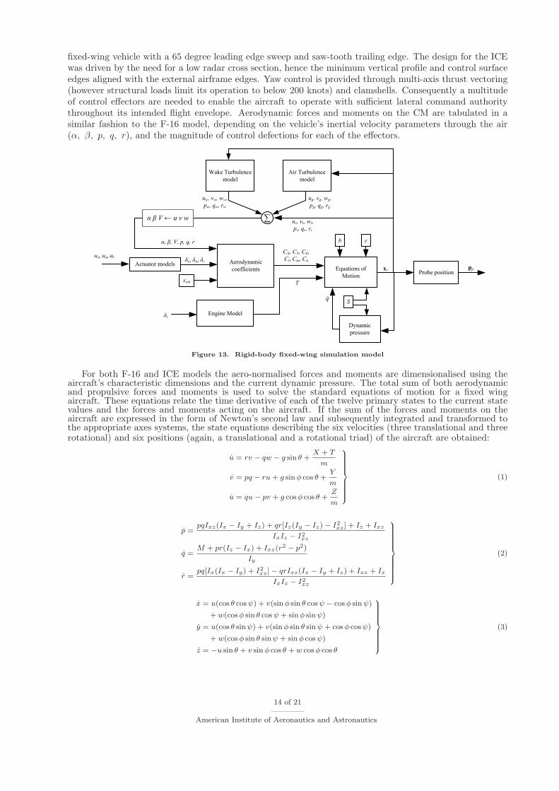
fixed-wing vehicle with a 65 degree leading edge sweep and saw-tooth trailing edge. The design for the ICEwas driven by the need for a low radar cross section, hence the minimum vertical profile and control surfaceedges aligned with the external airframe edges. Yaw control is provided through multi-axis thrust vectoring(however structural loads limit its operation to below 200 knots) and clamshells. Consequently a multitudeof control effectors are needed to enable the aircraft to operate with sufficient lateral command authoritythroughout its intended flight envelope. Aerodynamic forces and moments on the CM are tabulated in asimilar fashion to the F-16 model, depending on the vehicle’s inertial velocity parameters through the air(α, β, p, q, r), and the magnitude of control defections for each of the effectors.

ur, vr, wr,

pr, qr, rr

uw, vw, ww,

pw, qw, rw

pp

α, β, V, p, q, r

xr

q

T

δt

ug, vg, wg,

pg, qg, rg

Engine Model

∑

CX, CY, CZ,

Cl, Cm, Cn

Probe position

Air Turbulence

model

δe, δa, δrActuator models

Equations of

Motion

Aerodynamic

coefficients

xcm

b c

S

ue, ua, ur

Wake Turbulence

model

α β V ← u v w

Dynamic

pressure

Figure 13. Rigid-body fixed-wing simulation model

For both F-16 and ICE models the aero-normalised forces and moments are dimensionalised using theaircraft’s characteristic dimensions and the current dynamic pressure. The total sum of both aerodynamicand propulsive forces and moments is used to solve the standard equations of motion for a fixed wingaircraft. These equations relate the time derivative of each of the twelve primary states to the current statevalues and the forces and moments acting on the aircraft. If the sum of the forces and moments on theaircraft are expressed in the form of Newton’s second law and subsequently integrated and transformed tothe appropriate axes systems, the state equations describing the six velocities (three translational and threerotational) and six positions (again, a translational and a rotational triad) of the aircraft are obtained:

u = rv − qw − g sin θ +X + T

m

v = pq − ru+ g sinφ cos θ +Y

m

u = qu− pv + g cosφ cos θ +Z

m

(1)

p =pqIxz(Ix − Iy + Iz) + qr[Iz(Iy − Iz) − I2

xz] + Iz + Ixz

IxIz − I2xz

q =M + pr(Iz − Ix) + Ixz(r2 − p2)

Iy

r =pq[Ix(Ix − Iy) + I2

xz] − qrIxz(Ix − Iy + Iz) + Ixz + Ix

IxIz − I2xz

(2)

x = u(cos θ cosψ) + v(sinφ sin θ cosψ − cosφ sinψ)

+ w(cosφ sin θ cosψ + sinφ sinψ)

y = u(cos θ sinψ) + v(sinφ sin θ sinψ + cosφ cosψ)

+ w(cosφ sin θ sinψ + sinφ cosψ)

z = −u sin θ + v sinφ cos θ + w cosφ cos θ

(3)

14 of 21


φ = p+ tan θ(q sinφ+ r cosφ)

θ = q cosφ− r sinφ

ψ =q sinφ+ r cosφ

cos θ

(4)

The translational velocity equations are transformed into the wind axes to obtain equations of motion forthe angle of attack, sideslip angle, and total airspeed:

V =uV cosα cosβ + vV sin β + wV sinα cos β

V

β =(V v − V V sinβ) cos β

V 2 cos2 α cos2 β + V 2 sin2 α cos2 β

α =wV cosα cosβ − uV sinα cosβ

V 2 cos2 α cos2 β + V 2 sin2 α cos2 β

With the solution to these states the position of the probe nozzle is then calculated taking into accountrotations about the CM. Sufficient accuracy is obtained in the simulation model solving these using a third-order Runge-Kutta algorithm with a time step of 10 ms.

VI.B. Air turbulence

Additional intermittent forces and moments on aero-objects comes from atmospheric instabilities relating togradients in temperature, pressure, and velocity, resulting in deviations in the air flow from the free stream.Turbulence is observed in individual patches and is characterised by random, homogenous, and isotropicbehaviour. It is normally modelled by passing white noise with unity spectral density through a low-passshaping filter that gives the desired output spectrum.

VI.B.1. Mathematical representation

The continuous Dryden form is used, being convenient in that it has rational power spectral densities makingmodelling far simpler49

φu(ω) =2σ2

uLu

πU0

1

1 +(

LuωU0

)2

φv(ω) =σ2

vLv

πU0

1 + 3(

LvωU0

)2

[

1 +(

LvωU0

)2]2

φw(ω) =σ2

wLw

πU0

1 + 3(

LwωU0

)2

[

1 +(

LwωU0

)2]2

(5)

where

σ(·) are the gust intensities,

L(·) are the turbulence scales,

U0 is the still-air aircraft velocity, and

ω is the turbulence frequency

By assuming that the turbulence varies linearly over the aircraft’s surfaces the aerodynamic effect thatis equivalent to an inertial rotation of the aircraft can also be modelled. This leads to spectral densities for

15 of 21


the rotational affects of gusts which, for rigid airframes, can be simplified for moderate angles of attack:50

φp(ω) =σ2

w

U0Lw

0.8(

πLw

4b

)1

3

1 +(

4bωπU0

)2

φq(ω) =−

(

ωU0

)2

1 +(

3bωπU0

)2 φv(ω)

φr(ω) =−

(

ωU0

)2

1 +(

4bωπU0

)2 φw(ω)

(6)

where b is the wingspan. Equations (5) and (6) are solved in the time domain by transforming them intocanonical state-space form so the turbulent velocity components can be summed to the aircraft’s inertialvelocity parts prior to solving the equations of motion. For example, in the longitudinal axes the axial andvertical gust perturbations (ug, wg) can be written and solved with

su

sw1

sw2

=

−U0

Lu0 0

0 0 1

0(

U0

Lw

)2

−2U0

Lw

su

sw1

sw2

+

δu

0

δw

[

ug

wg

]

=

σu

√

2U0

πLu0 0

0 σw√π

(

U0

Lw

)3

2

σw

√

3U0

πLw

su

sw1

sw2

(7)

where s(·) are the transfer function states and δ(·) are the white noise disturbance source. Current airspeedand altitude values throughout the simulation are used to calculate the filters. The values for the turbulencescales are chosen equal (1750 ft), as are the values for each gust intensity in order to satisfy the mathematicalrequirement for isotropic turbulence.49 For altitudes above 2000 ft the turbulence intensities, σ, are relatedto a probability of exceedance: a lower probability represents more severe turbulence, as indicated in Figure14 .

80

70

60

50

40

30

20

10

5 10 15 20 25

RMS Turbulence Amplitude σ (ft/s TAS)

Alt

itu

de

(th

ou

san

ds

of

feet

) Probability of

Exceedance

10−2

10−3

10−4

Figure 14. Turbulence severity and exceedance probabilities.

16 of 21


VI.B.2. Implementation

After filtering the white noise the resulting turbulent velocity components are summed with the aircraft’sinertial velocity components from the aircraft, prior to the calculation of the aerodynamic forces and mo-ments. This requires a temporary transformation of the aircraft’s aerodynamic velocity (α, β, V ) from windto body axes in order to apply the changes. Since there is a correlation between the turbulence in pitch andnormal turbulence (wg, qg) and in yaw and lateral turbulence (rg, vg),

49 the same white noise generator isused for each parameter of the correlation pair.

As far as air turbulence modelling is concerned, the Dryden gust model has become the de facto represen-tation for stochastic air turbulence. There are however two limitations with the Dryden model: Firstly thespectrum density decays at ω/V −2 at high frequencies,51 greater than the observed rate of ω/V −5/3. Thisdiscrepancy would be of concern if high frequency motion, such as structural bending modes, where beingconsidered. The spectral densities for the rotational disturbances are also valid only for low frequencies sincethe assumption of linear variation of turbulence across the aircraft’s surfaces only holds when the wavelengthof the disturbance is greater than 8 times the length of the aircraft.50 Secondly, the time-domain-transformedturbulence has, like the white input noise, a Gaussian probability distribution. Atmospheric turbulence isnot considered to have a normal distribution; this can be addressed by randomly modulating the filter outputto obtain a more realistic probability distribution.52

Also developed for use in the simulation are a coupled hose-drogue model, with integrated bow waveeffects. The inclusion of these elements, the wake vortex model, along with all the elements above serves toprovide a high fidelity simulation suited to the proposed technology validation purposes.

VI.C. Real Time Robotic Simulation

The position outputs from the flight dynamics simulation are used here to assess the performance of thereal time motion control described in the foregoing sections. In this case, a datum position is chosen fixedrelative to the tanker aircraft, and the probe and drogue motion relative to this datum are reproducedindependently by R2 and R1 respectively. One degree of redundancy remains: the track motion. This isresolved by separating the motion of the drogue into high- and low-frequency components; the robot axes areused to perform the high-frequency motion and the track moves the robot base to provide the low-frequency,quasi-static response and give the probe its full longitudinal operational range. A time constant of 1Hz isused for this filtering. Only the high level interface is used in these tests, in anticipation of the completionof the full, combined high- and low-level interface system.

The start point of the simulations is reached through a smooth transition from the default starting posi-tion, 5500 mm directly aft of the datum position (itself 500 mm aft of the drogue canopy starting position).This transition is effected with a triangular velocity profile to accelerate and decelerate uniformly betweenthe default and start positions. The simulation is paused throughout the transition and is commenced froma stationary pose at the start position. For initial tests, safety limits are imposed on the relative positions ofthe probe and drogue to ensure that the two pieces of hardware do not impact as the simulation progressesthrough the contact stage. The forward-aft motion of the probe is transformed using the following equation:

x2 =

{

x2 , x2 < xsafexsafe

2−x2/xsafe, x2 ≥ xsafe

(8)

where x2 is the demanded x-position for R2 relative to the demanded drogue position, x2 is the respectiveposition from the simulation, and xsafe is the distance at which the position modulation begins (again withrespect to the drogue). The output of this function approaches zero smoothly and asymptotically as thedemanded position increases past xsafe, with a continuous derivative at the point xsafe (and elsewhere).Behind xsafe the probe motion is mapped directly to the robot motion. A value of xsafe = −1000mm isused for the tests conducted here.

The results presented in this section illustrate the response characteristics of the robot motion. It wasexpected that a small delay would be observed as a result of the motion path buffering, and that artefacts ofthe interpolation around position data points would be seen. What was not clear in advance was what thedynamic response of the motors and their proprietary feedback/feedforward controllers would be. To testthese effects, a predetermined motion path was implemented.

For the first tests a script reads position and orientation data from an ASCII file and executes thecorresponding motion instructions at a rate of 50 Hz. The target points are provided from an AAAR

17 of 21


0 10 20 30 40 50 60−1000

0

1000

2000

3000

4000

5000

6000

time (s)

posi

tion

(mm

)

x2simy2simz2simx2measy2measz2meas

(a) Absolute positions from the simulated data and fromthe measured robot positions.

0 10 20 30 40 50 60−20

0

20

40

60

80

100

time (s)

posi

tion

erro

r (m

m)

x2y2z2

(b) Position error for the robot motion relative to the pre-scribed simulation data motion path.

Figure 15. Positional data from the real time flight simulation.

Figure 16. Results of the real time simulation running on the robots

18 of 21


simulation. Measurements of the actual robot positions along with time stamps provided by the robotcontroller are streamed over a TCP/IP connection, in this case to a separate PC, at a rate of 50 Hz, andrecorded. The resulting data can not be synchronised with the move instructions, but for this analysis hasbeen aligned with the prescribed motion path by minimising an error function. It is thus not possible toidentify the static delay component of the response, but all other features of the response should be apparent.

Figure 15(a) shows the absolute position data, including the 3DOF translational position output fromthe simulation overlaid with the measured response of the robots. At this scale the lines appear coincident.The simulation shows a position hold approximately 5 m aft of the drogue, followed by an approach tothe pre-contact position, which is again held approximately 2 m aft of the drogue, and finishing with anaggressive engagement. The simulated refuelling procedure is conducted in light turbulence.

Figure 15(b) shows the position error from these plots. It is interesting to note that any effects fromcorner path artefacts are indiscernible in the presence of other disturbances. The large peak at approximately30 s corresponds with the rapid approach of the receiver aircraft to the pre-contact position. A similar sharprise is seen at the end of the plot where the final engagement is made. Although these errors are presentedhere as positional errors, they are found to be better described as temporal discrepancies; the differences seenare the result of a lag between the demanded motion and the measured robot position when moving at highspeeds. What is not apparent in this figure, but can be determined from close examination of Figure 15(a),is that while the robot motion lags the demand at some points, it leads the demand at others. This leadmay not be a true lead, as the alignment of the two signals in this case is not guaranteed, but it nonethelesspoints to a variable frequency response that could be characterised to the ends of further improving theperformance using a feedforward control approach.

Further tests were conducted, this time using the full real-time configuration, and allowing delays in themotion control to be analysed properly. Figure 16 shows the results of these simulations, where the halfsecond delay is clearly visible.

VII. Conclusions

Three control topologies have been discussed for real time control of a large scale robotic facility used toconduct hybrid tests. Deterministic control schemes have been developed to interface with the proprietaryrobot controller at a high level, but it has been shown that the latency in this interface exceeds 500ms and istoo high for closed loop real time simulations. Preliminary tests of a low level interface have been conducted,showing latencies closer to 20ms, and a control topology has been outlined to maintain safe control of thelarge and powerful robots while compensating for the delays in the high-level approach.

Physical considerations of using a 6DOF robot arm for this type of application are discussed, and mea-sured performance indices are presented, showing that there are optimal operating points for the machines.Motion path optimisation schemes are outlined, taking advantage of the freedom offered when simulatingrelative motion between two bodies.

The initial results from the real-time open loop flight dynamics simulations are promising, with goodreproduction of the position demands, but using the high-level interface results in unacceptable latencies.The full, closed-loop simulations will rely on completion of the low-level interface.

Future work will focus in the short term on the completion of the low-level interface to the robot controller,and development of the motion path optimisation. The outcome of this development work will be the facilityto implement high-bandwidth, closed-loop, hybrid simulations in a robust, stable, and realistic manner. Thiswill lead to tests of novel sensing and control technologies for autonomous air-to-air refuelling. Beyond thisthe focus will be shifted towards including force feedback capabilities and developing methods for simulatingdiscontinuous contact events.

Acknowledgments

This work is funded by Cobham Mission Equipment as part of the ASTRAEA Programme. The AS-TRAEA programme is co-funded by AOS, BAE Systems, Cobham, EADS Cassidian, QinetiQ, Rolls-Royce,Thales, the Technology Strategy Board, the Welsh Assembly Government and Scottish Enterprise. Website:http://www.astraea.aero/ The authors would like to thank Anders Robertsson, Anders Blomdell and KlasNilsson of the University of Lund, Sweden, for the use of their ORCA software suite and for their extensivehelp in setting it up.

19 of 21


References

1Newhook, P. and Eng, P., “A Robotic Simulator for Satellite Operations,” Proceedings of the 6 th Interna, tionalSymposium on Artificial Intelligence and Robotics & Automation in Space: i-SAIRAS, June 18-22(2001), 2001.

2Kaiser, C., Rank, P., Krenn, R., and Landzettel, K., “Simulation of the docking phase for the SMART-OLEV satelliteservicing mission,” i-SAIRAS: Int. Symposium on Artificial Intelligence, Robotics and Automation in Space, 2008, pp. 26–29.

3“ATP-56(B) Air-to-Air Refuelling,” NATO, 2010.4Leisy, C. J., “Aircraft Interconnecting Mechanism,” 1953.5Latimer-Needham, C. H., “APPARATUS FOR AIRCRAFT-REFUELLING IN FLIGHT AND AIRCRAFT TOWING,”

Aug. 30 1955.6Venkataramanan, S. and Dogan, A., “Dynamic Effects of Trailing Vortex with Turbulence & Time-varying Inertia in

Aerial Refueling,” Proceeedings of the AIAA Atmospheric Flight Mechanics Conference and Exhibit , Providence, Rhode Island,August 2004.

7Kim, E., Dogan, A., and Blake, W., “Control of a receiver aircraft relative to the tanker in racetrack maneuver,” AIAAGuidance, Navigation and Control Conference and Exhibit , Keystone, Colorado, August 2006.

8Wang, J., Patel, V., Cao, C., Hovakimyan, N., and Lavretsky, E., “L1 adaptive neural network controller for autonomousaerial refueling with guaranteed transient performance,” AIAA Guidance, Navigation and Control Conference and Exhibit ,Keystone, Colorado, August 2006.

9Wang, J., Patel, V., Cao, C., Hovakimyan, N., and Lavretsky, E., “Novel L1 Adaptive Control Methodology for AerialRefueling with Guaranteed Transient Performance,” Journal of Guidance, Control, and Dynamics, Vol. 31, No. 1, 2008.

10Wang, J., Patel, V. V., Cao, C., Hovakimyan, N., and Lavretsky, E., “Verifiable L1 Adaptive Controller for AerialRefueling,” AIAA Guidance, Navigation and Control Conference and Exhibit , Hilton Head, South Carolina, August 2007.

11Stephanyan, V., Lavretsky, E., and Hovakimyan, N., “A Differential Game approach to aerial refuelling autopilot design,”IEEE International Conference on Decision and Control , Maui, Hawaii, December 2003.

12Stephanyan, V., Lavretsky, E., and Hovakimyan, N., “Aerial Refuelling Autopilot Design Methodology: Application toF-16 Aircraft Model,” AIAA Guidance, Navigation and Control Conference and Exhibit , Providence, Rhode Island, August2004.

13Ding, J., Sprinkle, J., Sastry, S. S., and Tomlin, C. J., “Reachability calculations for automated aerial refuelling,”Procedings of the IEEE Conference on Decision and Control , Cancun, Mexico, December 2008.

14Elliot, C. M. and Dogan, A., “Investigating Nonlinear Control Architecture Options for Aerial Refueling,” AIAA Guid-ance, Navigation and Control Conference and Exhibition, Toronto, Canada, August 2010.

15Marwaha, A. D., Valasek, J., and Narang, A., “Fault Tolerant SAMI for Vision-Based Probe and Drogue AutonomousAerial Refueling,” AIAA Infortech@Aerospace and AIAA Unmanned... Unlimited Conference, Seattle, Washington, April 2009.

16Wang, J., Hovakimyan, N., and Cao, C., “L1 Adaptive Augmentation of Gain-Scheduled Controller for Racetrack Ma-neuver in Aerial Refueling,” AIAA Guidance, Navigation and Control Conference and Exhibit , Chicago, Illinois, August 2009.

17Dogan, A., Sato, S., and Blake, W., “Flight control and simulation for aerial refueling,” 2005 AIAA Guidance, Navigation,and Control Conference and Exhibit , San Francisco, California, 2005, pp. 1–15.

18RO, K. and KAMMAN, J., “Modeling and Simulation of Hose-Paradrogue Aerial Refueling Systems,” Journal of guidance,control, and dynamics, Vol. 33, No. 1, 2010, pp. 53–63.

19Ross, S., Menza, M. D., Waddell, Jr., E. T., Mainstone, A. P., and Velez, J., “Demonstration of a Control Algorithm forAutonomous Aerial Refueling (Project “No Gyro”),” Tech. Rep. AFFTC-TIM-05-10, AIR FORCE FLIGHT TEST CENTEREDWARDS AFB CA, December 2005.

20Ross, S., Pachter, M., Jacques, D., Kish, B., and Millman, D., “Autonomous aerial refueling based on the tanker referenceframe,” Aerospace Conference, 2006 IEEE , IEEE, 2006, pp. 22–pp.

21Hansen, J., Murray, J., and Campos, N., “The NASA Dryden AAR Project- A flight test approach to an aerial refuelingsystem,” AIAA Atmospheric Flight Mechanics Conference and Exhibit, 2004.

22Hansen, J., Murray, J., and Campos, N., “The NASA Dryden flight test approach to an aerial refueling system,” Tech.Rep. NASA/TM-2005-212859, National Aeronautics and Space Administration, February 2005.

23Dibley, R., Allen, M., Nabaa, N., and Sparks, N., “Autonomous Airborne Refueling Demonstration, Phase I Flight-TestResults,” Tech. Rep. NASA/TM-2007-214632, National Aeronautics and Space Administration, December 2007.

24Weaver, A. D., Using predictive rendering as a vision-aided technique for autonomous aerial refueling, MS Thesis, AirForce Institute of Technology, March 2009.

25Williamson, W. R., Glenn, G. J., Dang, V. T., Speyer, J. L., Stecko, S. M., and Takacs, J. M., “Sensor Fusion Appliedto Autonomous Aerial Refueling,” Journal of Guidance, Control, and Dynamics, Vol. 32, No. 1, 2009, pp. 262–275.

26Campa, G., Fravolini, M. L., Ficola, A., Napolitano, M. R., Seanor, B., and Perhinschi, M. G., “Autonomous AerialRefueling for UAVs Using a Combined GPS-Machine Vision Guidance,” AIAA Guidance, Navigation, and Control Conferenceand Exhibit , Providence, Rhode Island, August 2004.

27Fravolini, M. L., Ficola, A., Campa, G., Napolitano, M. R., and Seanor, B., “Modeling and control issues for autonomousaerial refueling for UAVs using a probe-drogue refueling system,” Aerospace Science and Technology, , No. 8, 2004, pp. 611–618.

28Mati, R., Pollini, L., Lunghi, A., Innocenti, M., and Campa, G., “Vision based autonomos probe and drogue refueling,”14th Mediterranean Conference on Control and Automation, 2006.

29Spencer, J. H., Optical tracking for relative positioning in automated aerial refueling, MS Thesis, Air Force Institute ofTechnology, March 2007.

30Mammarella, M., Campa, G., Napolitano, M. R., Fravolini, M. L., Gu, Y., and Perhinschi, M. G., “Machine vision/GPSintegration using EKF for the UAV aerial refueling problem,” IEEE Transactions on Systems, Man, and Cybernetics - part C:Applications and Reviews, Vol. 38, November 2008.

20 of 21


31Mammarella, M., Campa, G., Napolitano, M. R., Seanor, B., Fravolini, M. L., and Pollini, L., “GPS/MV based aerialrefueling for UAVs,” AIAA Guidance, Navigation and Control Conference and Exhibit , Honolulu, Hawaii, August 2008.

32Junkins, J. L., Schaub, H., and Hughes, D., “Non contact position and orientation measurement system and method,”US Patent 6,266,142, 2011.

33Valasek, J., G. K. K. J. T. M. J. L. and Hughes, D., “Vision-Based Sensor and Navigation System for Autonomous AirRefueling,” Proceeedings of the 1st AIAA Unmanned Aerospace Vehicles, Systems, Technologies, and Operations Conferenceand Workshop, Portsmouth, VA, 20-22 May 2002.

34Kimmett, J., Valasek, J., and Junkins, J. L., “Autonomous aerial refueling utilising a vision based navigation system,”AIAA GUidanc, Navigation, and Control Conference and Exhibit , Monterey, California, 5–8 August 2002.

35Kimmett, J., Valasek, J., and Junkins, J. L., “Vision based controller for autonomous aerial refueling,” Proceedings ofthe 2002 IEEE International Conference on Control Applications, Glasgow, Scotland, 2002.

36Tandale, M. D., Bowers, R., and Valasek, J. L., “Robust trajectory tracking controller for vision based probe and drogueautonomous aerial refueling,” AIAA Guidance, Navigation, and Control Conference and Exhibit , San Francisco, California,August 2005 2005.

37Pollini, L., Mati, R., and Innocenti, M., “Experimental evaluation of vision algorithms for formation flight and aerialrefueling,” AIAA Modeling and SImulation Technologies Conference and Exhibit , Providence, Rhode Island, August 2004.

38Pollini, L., Innocenti, M., and Mati, R., “Vision algorithms for formation flight and aerial refueling with optimal markerlabeling,” AIAA Modeling and SImulation Technologies Conference and Exhibit , San Francisco, California, August 2005.

39du Bois, J., Titurus, B., and Lieven, N., “Transfer Dynamics Cancellation in Real-Time Dynamic Substructuring,”International Conference on Noise and Vibration Engineering, ISMA2010 , Leuven, Belgium, 2010.

40Wallace, M., Wagg, D., Neild, S., Bunniss, P., Lieven, N., and Crewe, A., “Testing coupled rotor blade-lag dampervibration using real-time dynamic substructuring,” Journal of Sound and Vibration, Vol. 307, No. 3-5, 2007, pp. 737–754.

41Wallace, M., Wagg, D., and Neild, S., “An adaptive polynomial based forward prediction algorithm for multi-actuatorreal-time dynamic substructuring,” Proceedings of the Royal Society A: Mathematical, Physical and Engineering Science,Vol. 461, No. 2064, 2005, pp. 3807.

42Chen, C. and Ricles, J., “Analysis of actuator delay compensation methods for real-time testing,” Engineering Structures,Vol. 31, No. 11, 2009, pp. 2643–2655.

43Blomdell, A., Dressler, I., Nilsson, K., Robertsson, A., and Dressler, I., “Flexible application development and high-performance motion control based on external sensing and reconfiguration of abb industrial robot controllers,” Proc. of theworkshop of” Innovative Robot Control Architectures for Demanding (Research) ApplicationsHow to Modify and EnhanceCommercial Controllers”, the 2010 IEEE Int. Conf. on Robotics and Automation (ICRA2010), 2010, pp. 62–66.

44Sidhu, S., Performance Characterisation and Motion Optimisation for a Relative Motion Robotic Facility, Master’sthesis, University of Bristol, UK, 2012.

45Mao, W. and Eke, F., “A Survey of the Dynamics and Control of Aircraf During Aerial Refueling,” Nonlinear Dynamicsand Systems Theory, Vol. 8, No. 4, 2008, pp. 375–388.

46Stevens, B. L. and Lewis, F. L., Aircraft Control and Simulation, John Wiley & Sons, USA, 2nd ed., 2003.47Nguyen, L. T., Ogburn, M. E., Gilbert, W. P., Kibler, K. S., Brown, P. W., and Deal, P. L., “Simulator Study of

Stall/Post-Stall Characteristics of a Fighter Airplane with Relaxed Longitudinal Static Stability,” Nasa tp 1538, washington,d. c., December 1979.

48Dorsett, K. M. and Mehl, D. R., “Innovative Control Effectors (ICE),” Wl-tr-96-3043, Wright-Patterson Airforce Base,Ohio, January 1996.

49MIL-F-8785C, “Flying Qualitites of Piloted Aircraft,” Department of defense, usa, 1980.50Roskam, J., Airplane Flight Dynamics and Automatic Flight Controls, Roskam Aviation and Engineering Corporation,

1979.51Wang, S.-T. and Frost, W., “Atmospheric Turbulence Simulation Techniques With Application to Flight Analysis,” Nasa

cr 3305, 1980.52Justus, C. G., Campbell, C. W., L., D. M., and Johnson, D. L., “New Atmospheric Turbulence Model for Shuttle

Applications,” Nasa tm 4168, 1990.

21 of 21


control methodologies for relative motion reproduction...

Documents