S1

Control of Grafting Density and Distribution in Graft Polymers

by Living Ring-Opening Metathesis Copolymerization

Tzu-Pin Lin,† Alice B. Chang,† Hsiang-Yun Chen,† Allegra L. Liberman-Martin,† Christopher M.

Bates,‡,⊥ Matthew J. Voegtle,§ Christina A. Bauer,§ and Robert H. Grubbs*,†

†Division of Chemistry and Chemical Engineering, California Institute of Technology, Pasadena, California 91125,

United States ‡Materials Department and ⊥Department of Chemical Engineering, University of California, Santa Barbara,

California 93106, United States §Department of Chemistry, Whittier College, Whittier, California 90608, United States

SUPPORTING INFORMATION

S2

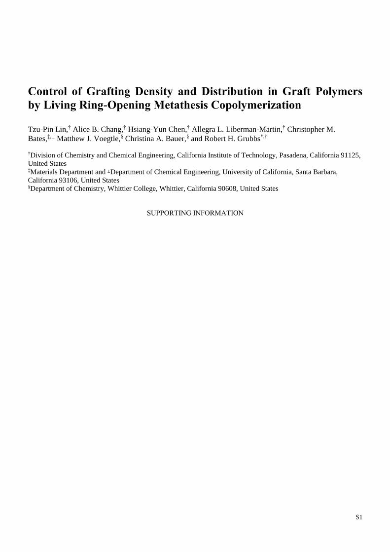
Figure S1. 1H NMR spectrum of PS in CDCl3.

S3

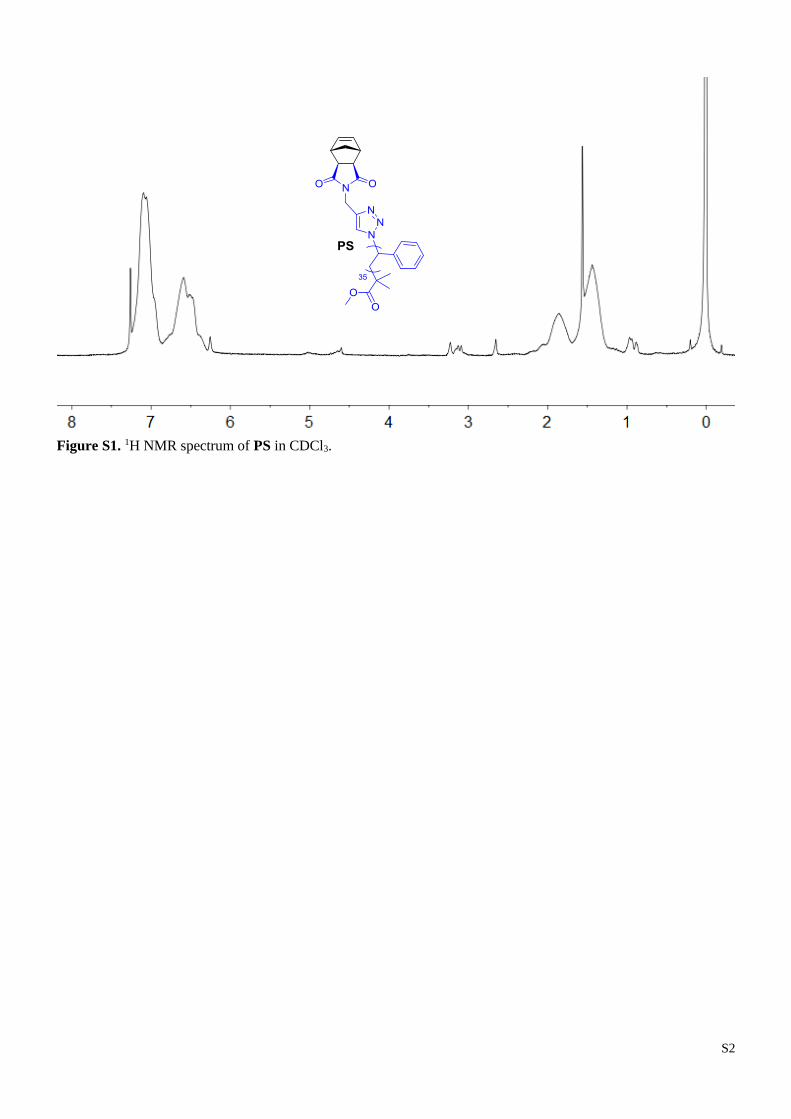
Figure S2. 1H NMR spectrum of PLA in CDCl3.

S4

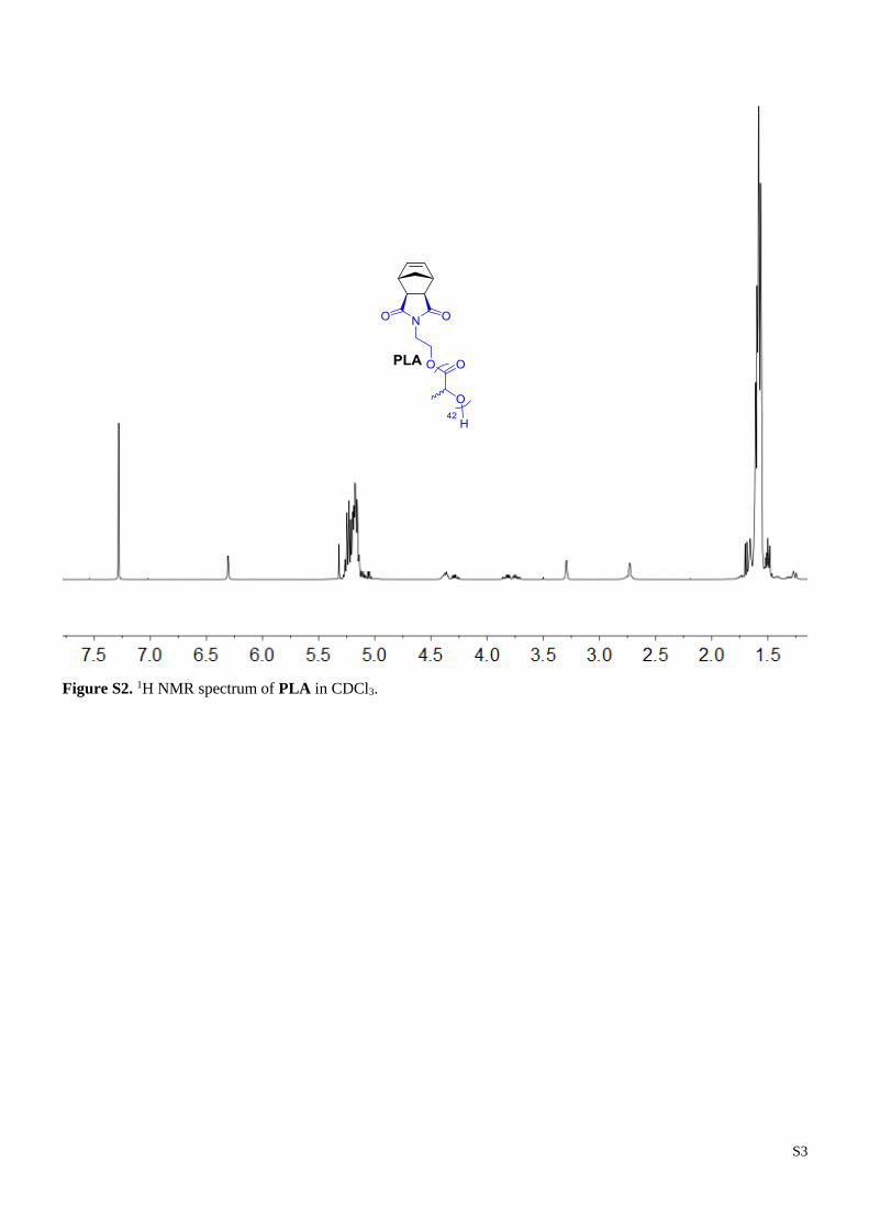
Figure S3. 1H NMR spectrum of PDMS in CDCl3.

S5

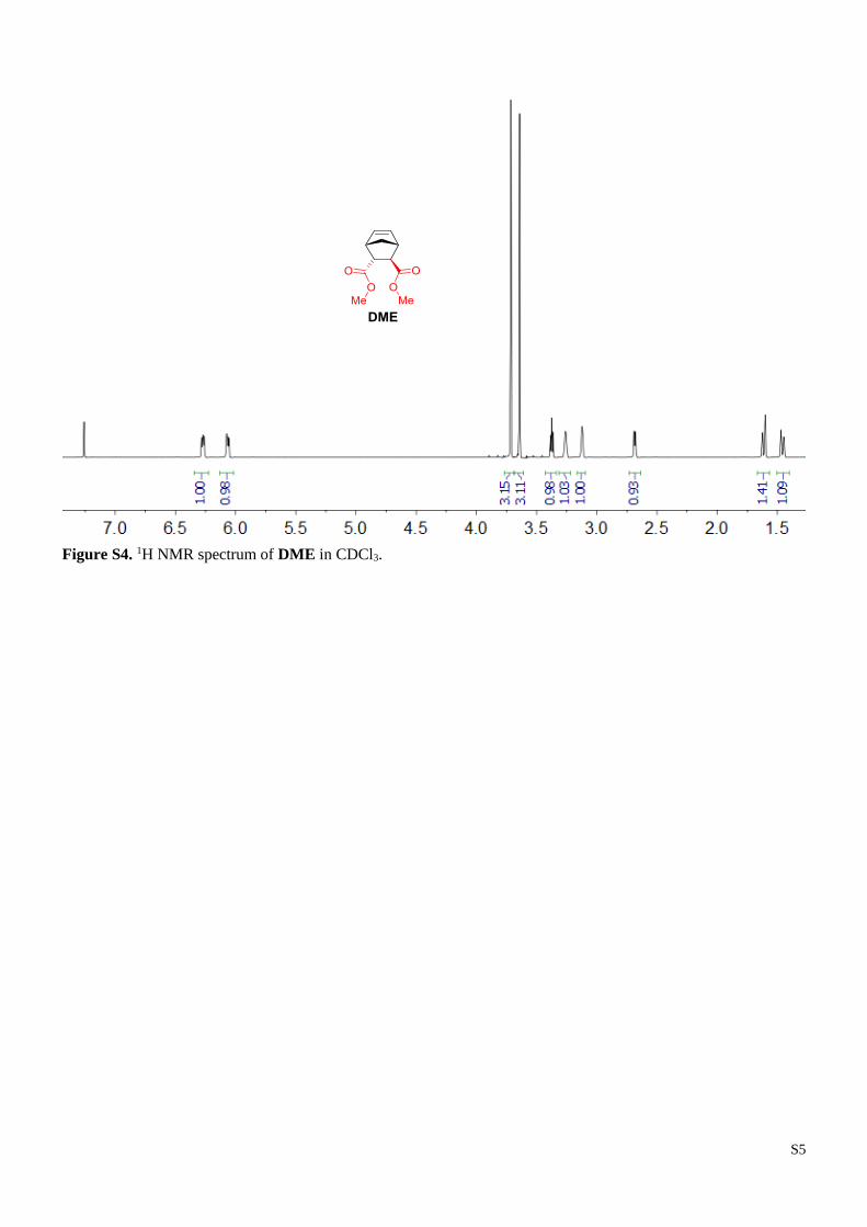
Figure S4. 1H NMR spectrum of DME in CDCl3.

S6

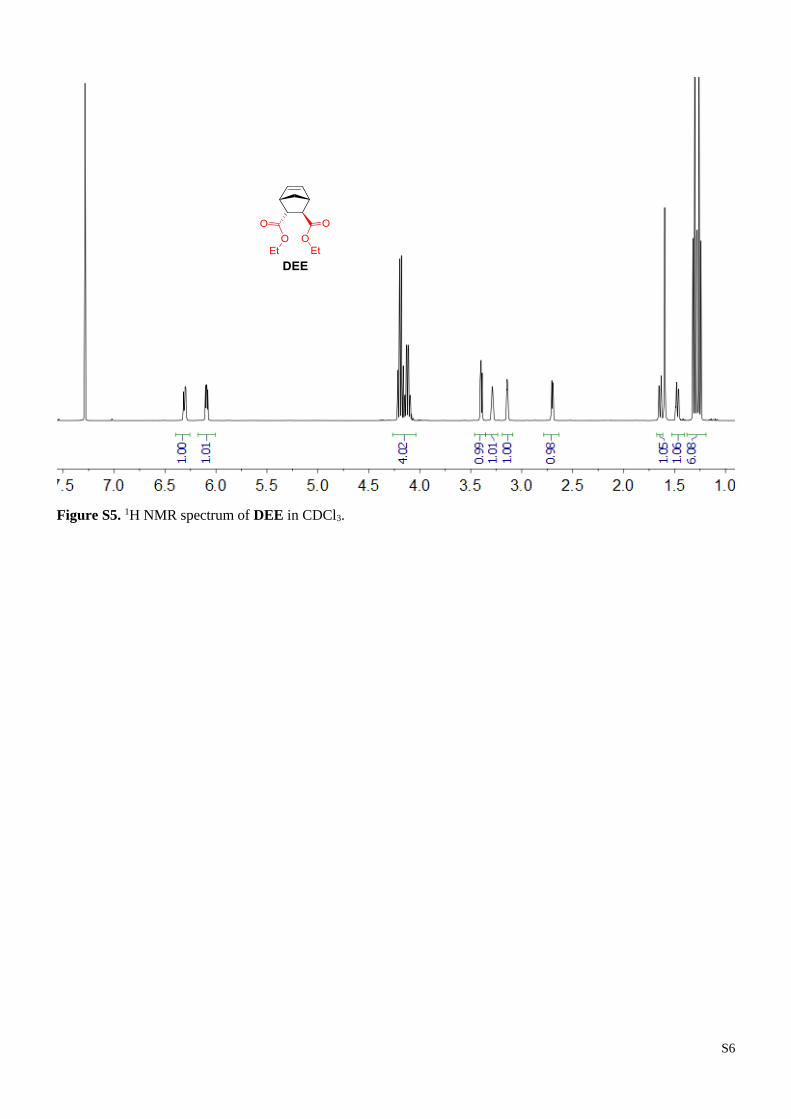
Figure S5. 1H NMR spectrum of DEE in CDCl3.

S7

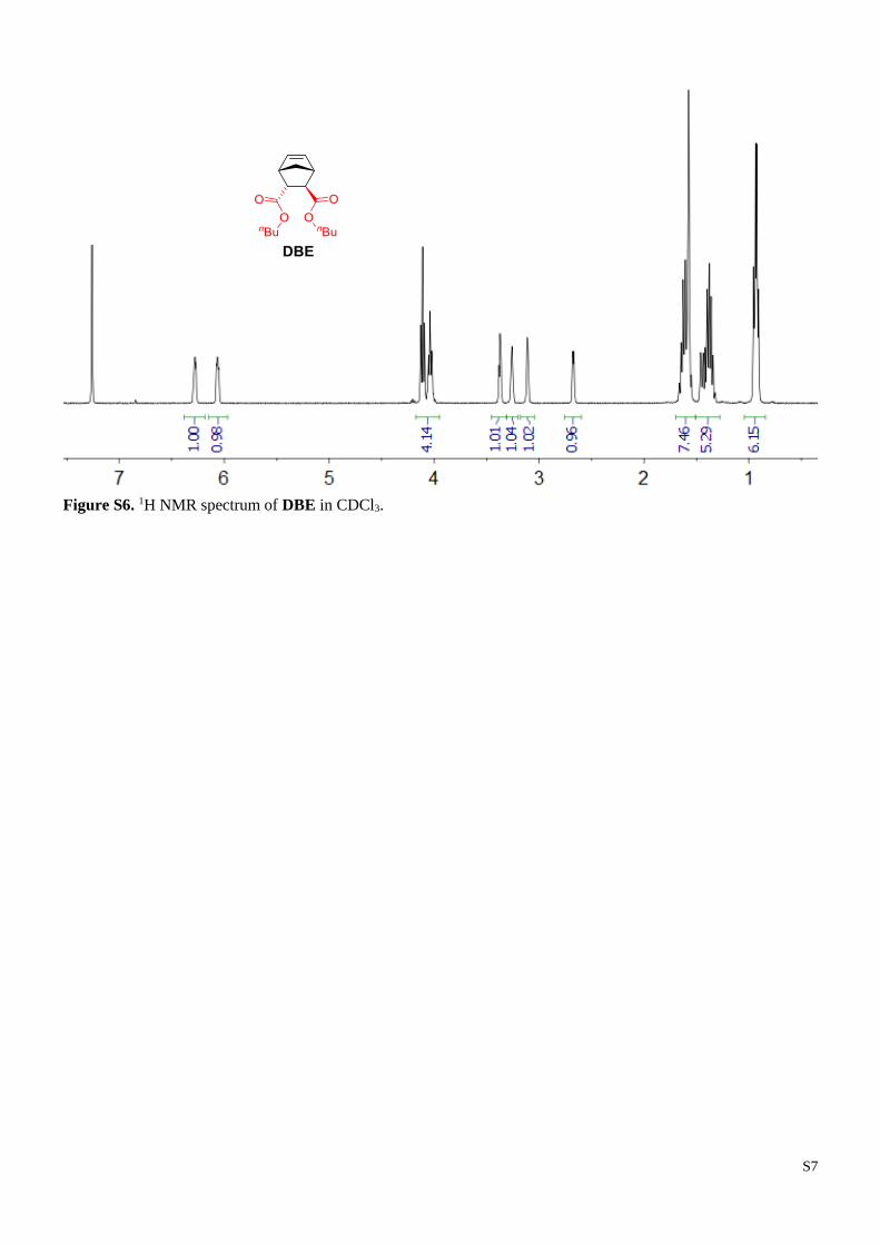
Figure S6. 1H NMR spectrum of DBE in CDCl3.

S8

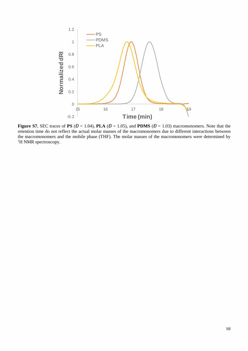
Figure S7. SEC traces of PS (Ɖ = 1.04), PLA (Ɖ = 1.05), and PDMS (Ɖ = 1.03) macromonomers. Note that the

retention time do not reflect the actual molar masses of the macromonomers due to different interactions between

the macromonomers and the mobile phase (THF). The molar masses of the macromonomers were determined by 1H NMR spectroscopy.

-0.2

0

0.2

0.4

0.6

0.8

1

1.2

15 16 17 18 19

No

rma

lize

d d

RI

Time (min)

PS

PDMS

PLA

S9

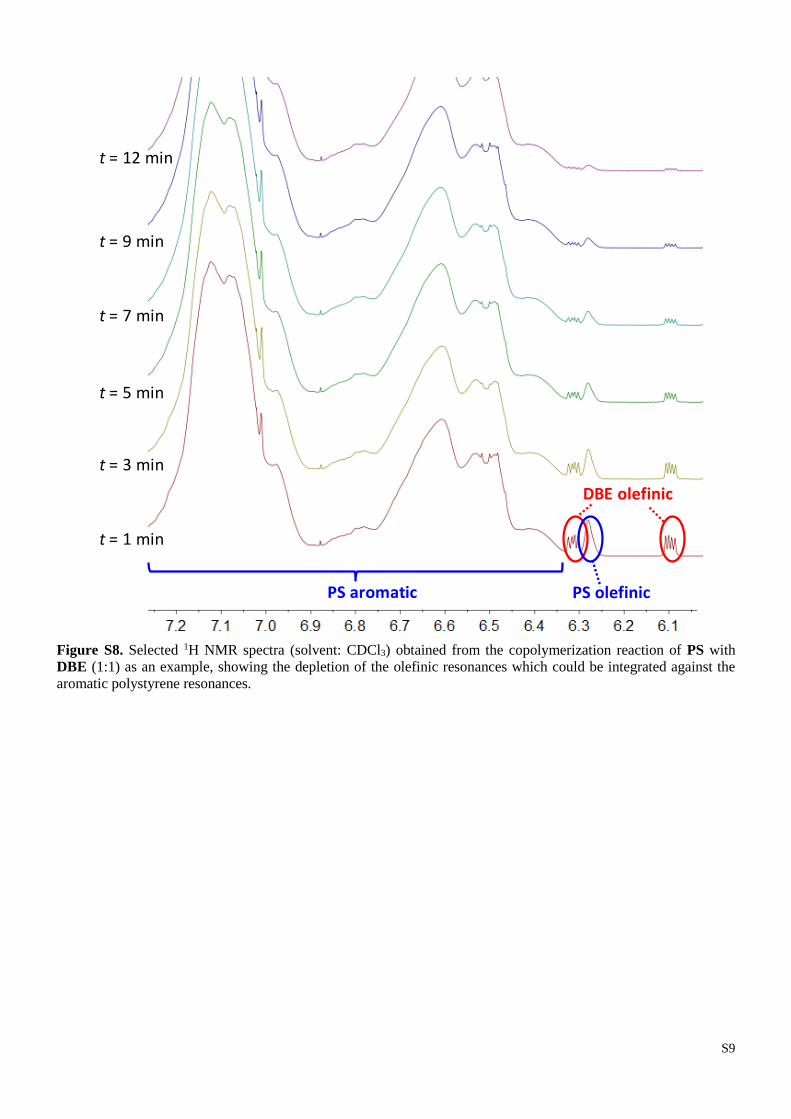
Figure S8. Selected 1H NMR spectra (solvent: CDCl3) obtained from the copolymerization reaction of PS with

DBE (1:1) as an example, showing the depletion of the olefinic resonances which could be integrated against the

aromatic polystyrene resonances.

PS aromatic PS olefinic

DBE olefinic

t = 1 min

t = 3 min

t = 5 min

t = 7 min

t = 9 min

t = 12 min

S10

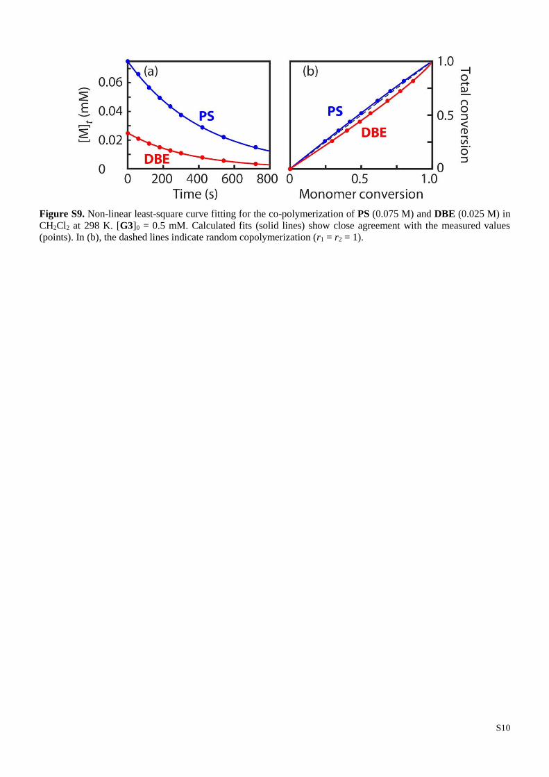
Figure S9. Non-linear least-square curve fitting for the co-polymerization of PS (0.075 M) and DBE (0.025 M) in

CH2Cl2 at 298 K. [G3]0 = 0.5 mM. Calculated fits (solid lines) show close agreement with the measured values

(points). In (b), the dashed lines indicate random copolymerization (r1 = r2 = 1).

S11

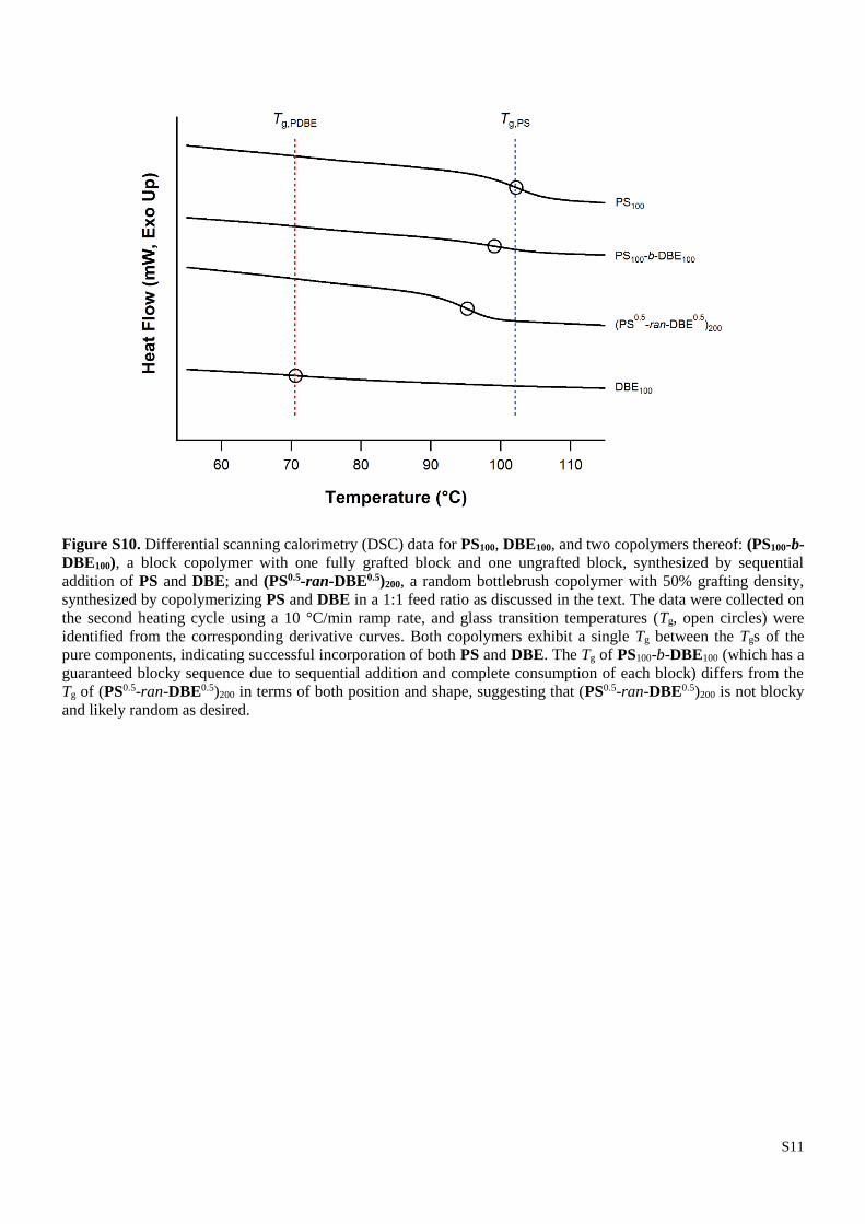
Figure S10. Differential scanning calorimetry (DSC) data for PS100, DBE100, and two copolymers thereof: (PS100-b-

DBE100), a block copolymer with one fully grafted block and one ungrafted block, synthesized by sequential

addition of PS and DBE; and (PS0.5-ran-DBE0.5)200, a random bottlebrush copolymer with 50% grafting density,

synthesized by copolymerizing PS and DBE in a 1:1 feed ratio as discussed in the text. The data were collected on

the second heating cycle using a 10 °C/min ramp rate, and glass transition temperatures (Tg, open circles) were

identified from the corresponding derivative curves. Both copolymers exhibit a single Tg between the Tgs of the

pure components, indicating successful incorporation of both PS and DBE. The Tg of PS100-b-DBE100 (which has a

guaranteed blocky sequence due to sequential addition and complete consumption of each block) differs from the

Tg of (PS0.5-ran-DBE0.5)200 in terms of both position and shape, suggesting that (PS0.5-ran-DBE0.5)200 is not blocky

and likely random as desired.

S12

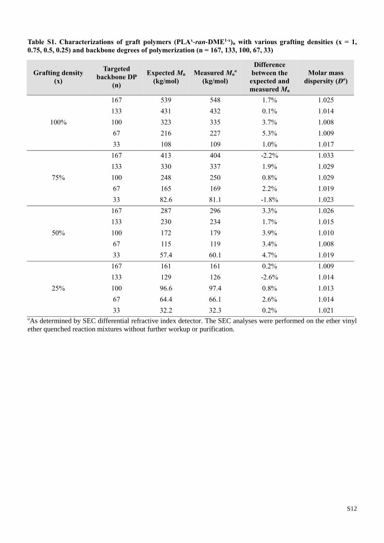
Table S1. Characterizations of graft polymers (PLAx-ran-DME1-x)n with various grafting densities (x = 1,

0.75, 0.5, 0.25) and backbone degrees of polymerization (n = 167, 133, 100, 67, 33)

Grafting density

(x)

Targeted

backbone DP

(n)

Expected Mn

(kg/mol)

Measured Mna

(kg/mol)

Difference

between the

expected and

measured Mn

Molar mass

dispersity (Ɖa)

100%

167 539 548 1.7% 1.025

133 431 432 0.1% 1.014

100 323 335 3.7% 1.008

67 216 227 5.3% 1.009

33 108 109 1.0% 1.017

75%

167 413 404 -2.2% 1.033

133 330 337 1.9% 1.029

100 248 250 0.8% 1.029

67 165 169 2.2% 1.019

33 82.6 81.1 -1.8% 1.023

50%

167 287 296 3.3% 1.026

133 230 234 1.7% 1.015

100 172 179 3.9% 1.010

67 115 119 3.4% 1.008

33 57.4 60.1 4.7% 1.019

25%

167 161 161 0.2% 1.009

133 129 126 -2.6% 1.014

100 96.6 97.4 0.8% 1.013

67 64.4 66.1 2.6% 1.014

33 32.2 32.3 0.2% 1.021 aAs determined by SEC differential refractive index detector. The SEC analyses were performed on the ether vinyl

ether quenched reaction mixtures without further workup or purification.

S13

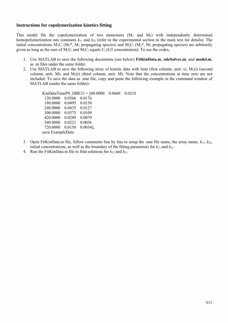
Instructions for copolymerization kinetics fitting

This model fits the copolymerization of two monomers (M1 and M2) with independently determined

homopolymerization rate constants k11 and k22 (refer to the experimental section in the main text for details). The

initial concentrations M1Ci (M1*, M1 propagating species) and M2Ci (M2*, M2 propagating species) are arbitrarily

given as long as the sum of M1Ci and M2Ci equals Ci (G3 concentration). To use the codes,

1. Use MATLAB to save the following documents (see below) FitKinData.m, odeSolver.m, and model.m,

as .m files under the same folder.

2. Use MATLAB to save the following array of kinetic data with time (first column, unit: s), M1(t) (second

column, unit: M), and M2(t) (third column, unit: M). Note that the concentrations at time zero are not

included. To save the data as .mat file, copy and paste the following example in the command window of

MATLAB (under the same folder):

KinDataTimePS_DBE31 = [60.0000 0.0660 0.0210

120.0000 0.0566 0.0176

180.0000 0.0495 0.0150

240.0000 0.0435 0.0127

300.0000 0.0375 0.0109

420.0000 0.0289 0.0079

540.0000 0.0221 0.0056

720.0000 0.0150 0.0034];

save ExampleData

3. Open FitKinData.m file, follow comments line by line to setup the .mat file name, the array name, k11, k22,

initial concentrations, as well as the boundary of the fitting parameters for k12 and k21.

4. Run the FitKinData.m file to find solutions for k12 and k21.

S14

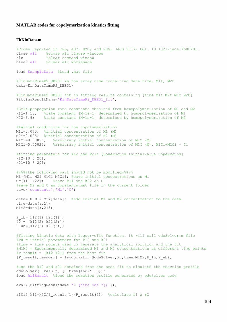
MATLAB codes for copolymerization kinetics fitting

FitKinData.m

%Codes reported in TPL, ABC, HYC, and RHG, JACS 2017, DOI: 10.1021/jacs.7b00791. close all %close all figure windows clc %clear command window clear all %clear all workspace

load ExampleData %Load .mat file

%KinDataTimePS_DBE31 is the array name containing data time, M1t, M2t data=KinDataTimePS_DBE31;

%KinDataTimePS_DBE31_fit is fitting results containing [time M1t M2t M1C M2C] FittingResultName='KinDataTimePS_DBE31_fit';

%Self-propagation rate constants obtained from homopolymerization of M1 and M2 k11=4.18; %rate constant (M-1s-1) determined by homopolymerization of M1 k22=6.9; %rate constant (M-1s-1) determined by homopolymerization of M2

%Initial conditions for the copolymerization M1i=0.075; %initial concentration of M1 (M) M2i=0.025; %initial concentration of M2 (M) M1Ci=0.00025; %arbitrary initial concentration of M1C (M) M2Ci=0.00025; %arbitrary initial concentration of M1C (M). M1Ci+M2Ci = Ci

%fitting parameters for k12 and k21: [LowerBound InitialValue UpperBound] k12=[0 5 20]; k21=[0 5 20];

%%%%%the following part should not be modified%%%%% Mi=[M1i M2i M1Ci M2Ci]; %save initial concentrations as Mi C=[k11 k22]; %save k11 and k22 as C %save Mi and C as constants.mat file in the current folder save('constants','Mi','C')

data=[0 M1i M2i;data]; %add initial M1 and M2 concentration to the data time=data(:,1); M1M2=data(:,2:3);

P_lb=[k12(1) k21(1)]; P0 = [k12(2) k21(2)]; P_ub=[k12(3) k21(3)];

%fitting kinetic data with lsqcurvefit function. It will call odeSolver.m file %P0 = initial parameters for k12 and k21 %time = time points used to generate the analytical solution and the fit %M1M2 = Experimentally determined M1 and M2 concentrations at different time points %P_result = [k12 k21] from the best fit [P_result,resnorm] = lsqcurvefit(@odeSolver,P0,time,M1M2,P_lb,P_ub);

%use the k12 and k21 obtained from the best fit to simulate the reaction profile odeSolver(P_result, [0 time(end)*1.3]); load AllResult %load the reaction profile generated by odeSolver code

eval([FittingResultName '= [time_ode Y];']);

r1Mr2=k11*k22/P_result(1)/P_result(2); %calculate r1 x r2

S15

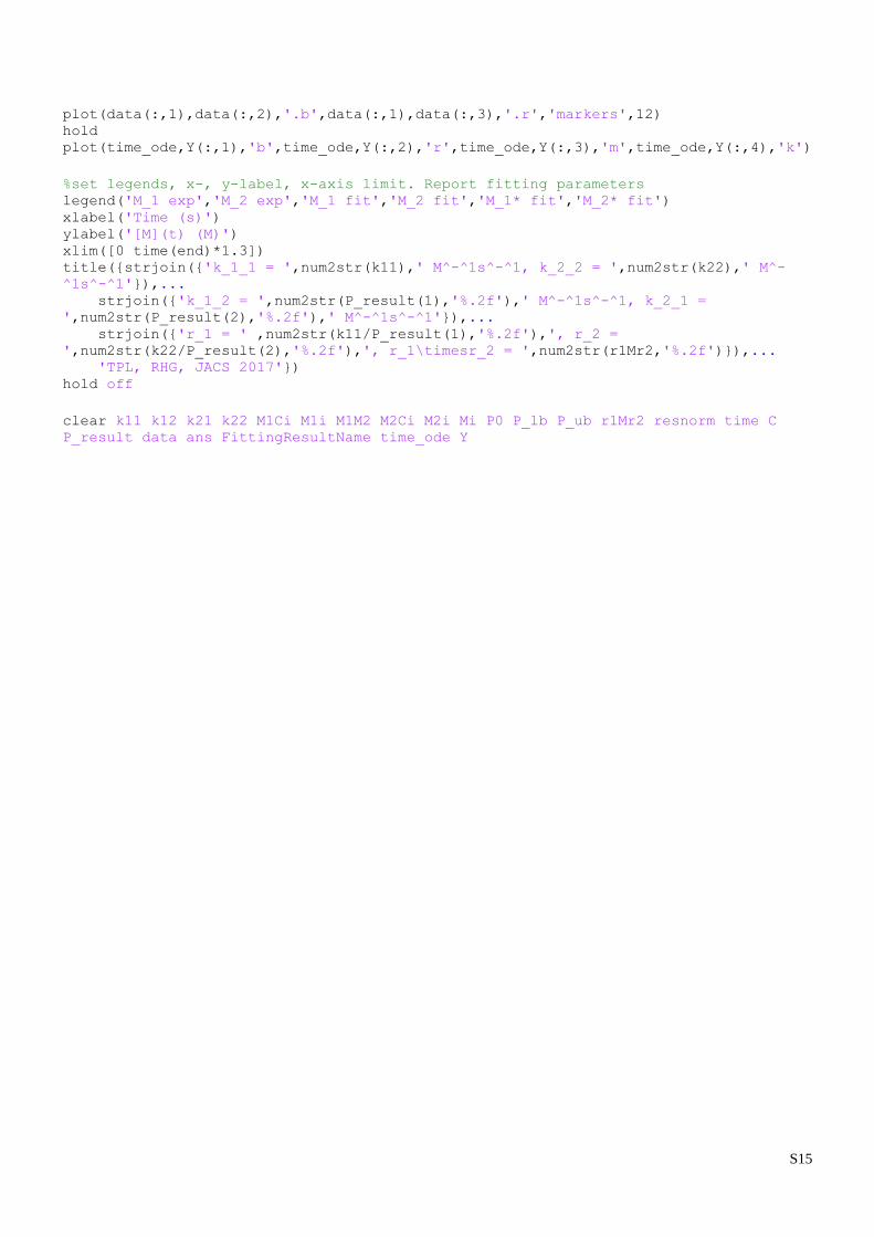
plot(data(:,1),data(:,2),'.b',data(:,1),data(:,3),'.r','markers',12) hold plot(time_ode,Y(:,1),'b',time_ode,Y(:,2),'r',time_ode,Y(:,3),'m',time_ode,Y(:,4),'k')

%set legends, x-, y-label, x-axis limit. Report fitting parameters legend('M_1 exp','M_2 exp','M_1 fit','M_2 fit','M_1* fit','M_2* fit') xlabel('Time (s)') ylabel('[M](t) (M)') xlim([0 time(end)*1.3]) title({strjoin({'k_1_1 = ',num2str(k11),' M^-^1s^-^1, k_2_2 = ',num2str(k22),' M^-

^1s^-^1'}),... strjoin({'k_1_2 = ',num2str(P_result(1),'%.2f'),' M^-^1s^-^1, k_2_1 =

',num2str(P_result(2),'%.2f'),' M^-^1s^-^1'}),... strjoin({'r_1 = ' ,num2str(k11/P_result(1),'%.2f'),', r_2 =

',num2str(k22/P_result(2),'%.2f'),', r_1\timesr_2 = ',num2str(r1Mr2,'%.2f')}),... 'TPL, RHG, JACS 2017'}) hold off

clear k11 k12 k21 k22 M1Ci M1i M1M2 M2Ci M2i Mi P0 P_lb P_ub r1Mr2 resnorm time C

P_result data ans FittingResultName time_ode Y

S16

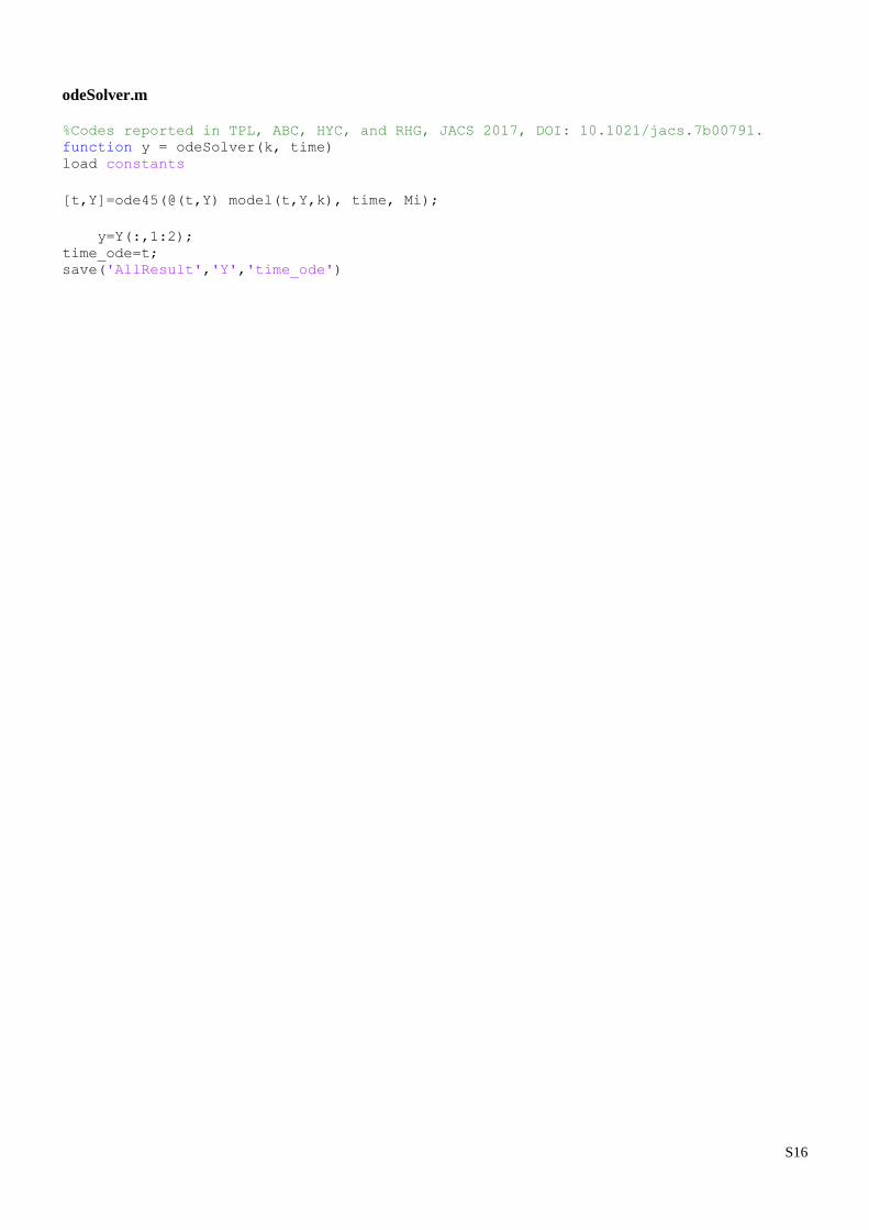
odeSolver.m

%Codes reported in TPL, ABC, HYC, and RHG, JACS 2017, DOI: 10.1021/jacs.7b00791. function y = odeSolver(k, time) load constants

[t,Y]=ode45(@(t,Y) model(t,Y,k), time, Mi);

y=Y(:,1:2); time_ode=t; save('AllResult','Y','time_ode')

S17

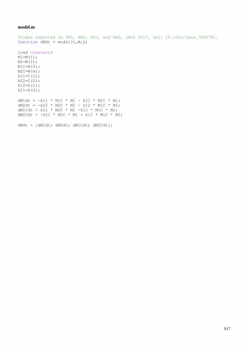
model.m

%Codes reported in TPL, ABC, HYC, and RHG, JACS 2017, DOI: 10.1021/jacs.7b00791. function dMdt = model(t,M,k)

load constants M1=M(1); M2=M(2); M1C=M(3); M2C=M(4); k11=C(1); k22=C(2); k12=k(1); k21=k(2);

dM1dt = -k11 * M1C * M1 - k21 * M2C * M1; dM2dt = -k22 * M2C * M2 - k12 * M1C * M2; dM1Cdt = k21 * M2C * M1 -k12 * M1C * M2; dM2Cdt = -k21 * M2C * M1 + k12 * M1C * M2;

dMdt = [dM1dt; dM2dt; dM1Cdt; dM2Cdt];