control of longitudinal pitch rate as aircraft center of
TRANSCRIPT

i
CONTROL OF LONGITUDINAL PITCH
RATE AS AIRCRAFT
CENTER OF GRAVITY
CHANGES
A Thesis
Presented to the Faculty of
California Polytechnic State University
San Luis Obispo
In Partial Fulfillment
of the Requirements for the Degree
Master of Science in Electrical Engineering
By
John Andres Cadwell Jr.
December 2010

ii
© 2010
John Andres Cadwell Jr.
ALL RIGHTS RESERVED
iii
APPROVAL
TITLE: Control of longitudinal pitch rate as aircraft center of gravity changes
AUTHOR: John Andres Cadwell Jr.
DATE SUBMITTED : December 2010
COMMITTEE CHAIR: Dr. Xiao-Hua Yu, PhD
COMMITTEE MEMBER: Dr. Dennis Derickson, PhD
COMMITTEE MEMBER: Dr. John Oliver, PhD
iv
ABSTRACT
In order for an aircraft to remain in stable flight, the center of gravity (CG) of an aircraft
must be located in front of the center of lift (CL). As the center of gravity moves rearward,
pitch stability decreases and the sensitivity to control input increases. This increase in
sensitivity is known as pitch gain variance. Minimizing the pitch gain variance results in an
aircraft with consistent handling characteristics across a broad range of center of gravity
locations.
This thesis focuses on the development and testing of an open loop computer simulation
model and a closed loop control system to minimize pitch axis gain variation as center of
gravity changes. DATCOM and MatLab are used to generate the open loop aircraft flight
model; then a closed loop PD (proportional-derivate) controller is designed based on Ziegler-
Nichols closed loop tuning methods. Computer simulation results show that the open loop
control system exhibited unacceptable pitch gain variance, and that the closed loop control
system not only minimizes gain variance, but also stabilizes the aircraft in all test cases. The
controller is also implemented in a Scorpio Miss 2 radio controlled aircraft using an onboard
microprocessor. Flight testing shows that performance is satisfactory.

v
ACKNOWLEDGEMENTS
Dr. Helen Yu
Thank you for seeing this work through to completion. I am grateful for your
services as thesis chair, and your efforts to see me finished.
Dr. Art MacCarley
Thank you for the opportunity to pursue research in an area of personal interest. You
have helped me to grow as a student and professional, providing academic tools
through coursework, and proving those tools with real world examples.
John Keith Carlin
It is with great fondness that I remember our time spent: The nearly nightly meals,
the dubious advice (technical and otherwise), and your ability to memorize. Your
friendship was instrumental. Thank you for your assistance documenting my
successes, speculating about improvements, and for not laughing too hard when I dug
holes in the ground with my airplanes. I’ll always have a fondness for park benches.
Without your skills, encouragement, and persistence, documenting my flight tests
would have been impossible. With the wisdom of a big-game hunter, you helped
maintain safety and discipline during those tests.

vi
Dr. John and Priscilla Cadwell
Thank you Mom and Dad. For your teaching, listening, love, and support. Without
your help I wouldn’t be where I am today. I’m grateful for having this opportunity,
and your understanding and encouragement have helped me through this degree.
Dad, you have inspired tremendous amounts of curiosity and intellectual pursuit.
You have consistently reminded me about the purposes of education. Thank you for
teaching me and providing the tools to learn.
Dr. George Moore, PhD, Agilent Fellow
Thank you George for your willingness to help someone you didn’t know. I came to
you at the last minute, and you gave your time freely to help me succeed. You helped
refine my approach, and gave me insight into subtleties of my modeling I would not
have recognized otherwise. You were encouraging and understanding to a fault.
Dr. Jillian Rae Cadwell
I could not define the word ‘friend’ more aptly than to look to you. Your
encouragement, love, constancy, and stability are felt every day. Thanks for talking
about MatLab for hours, for patiently listening, and for believing in me. Sometimes
in life, the way things are and the best that things could be seem the same. Those are
the times I’ve spent with you. Thank you for your friendship. Your patience is
immeasurable, and certainly beyond reason. Each day spent waiting was with hope.
The completion of this work turns hope into reality.

vii
Table of Contents
List of Tables…………………………………………………………….……...ix
List of Equations……………………………………………………..…..…......ix
List of Figures……………………………………………………………..….x-xi
Preface The Problem, Related Work, and The Scope
0-1 The Gain Changer………………………………………..……1
0-2 Previous Work……………………………………………..…..2
0-3 Statement of Objective………………………………………..3
0-4 Synopsis of Work………………………………………..…….4
Chapter 1 Pitch Control and Stability Theory
1-1 Overview of Pitch Control……………………………..……..7
1-2 Aircraft Stability………………………………………...…....8
Chapter 2 Plant Modeling
2-1 Elements of Pitch Behavior…………………………….…….10
2-2 DATCOM Modeling……………..………………………..….11
2-3 Longitudinal Equation of Motion……………………….…...15
2-4 Varying Transfer Function as a Plant Model………….…...16
2-5 Controllability……………………………………………........17
Chapter 3 Plant Development and Open Loop Simulation
3-1 Open Loop Simulation Methods and Objectives…………..18
3-2 Plant Development……….……………………………….….18
3-3 Open Loop Simulation Results..……………………….……24

viii
3-4 Open Loop Conclusions……... ……………………….….…..32
Chapter 4 Control System Development and Simulation
4-1 Control System Objectives……………………………..……..33
4-2 PD Control Law…………………………………………...…...33
4-3 Control System Structure……………………………..……....35
4-4 Control System Implementation ………………………..…....36
4-5 Closed Loop Simulation Methods and Objectives………..…38
4-6 Closed Loop Simulation Results…………………………...…39
4-7 Closed Loop Conclusions……………………………………...46
Chapter 5 Comparison of Open and Closed Loop
5-1 Open and Closed Loop Gain as a Function of the Location of CG
…………...…………………………………………….……….47
5-2 Pole Zero Plot Comparison……………………………………48
5-3 Response Comparison..…………………………………..……51
5-4 Controllability…………………………………………….……53
5-5 Comparison Conclusions..…………………………………….53
Chapter 6 Aircraft Flight Testing
6-1 Building the Model Airplane……………………………….….54
6-2 Flight Testing Methods………………………………………..54
6-3 Flight Testing Results……………………………………....…56
Chapter 7 Summary and Conclusions
7-1 Summary of Work Performed………………………………...58
7-2 Areas for Further Study………………………………………58

ix
7-3 Closing Remarks………………………………………….…....59
Cited References……………………………………………………………….61
Appendix A: Equipment Description
Appendix B: Aircraft Systems and Software
List of Tables
Table 2.1 Input Variables…………………………………………………..…12
Table 2.2 Model Parameters……………………………………………...…..12
Table 2.3 Output……………………………………………………………….13
Table 2.4 Calculated Longitudinal Forces and Moments…………………..14
List of Equations
Equation 2.1 Short Period Motion Description……………………….…….15
Equation 2.2 Pitch Rate of Change for Elevator Deflection……………….15
Equation 2.3 Simplified Transfer Function…………………………….…...16
Equation 2.5 Controllability Matrix……………………………………..….17
Equation 3.1 Open Loop DC Gain……………………………………….….24
Equation 3.2 Open Loop Gain Percentage Increase...………………….….31
Equation 4.1 PD Control Structure…………………………………………34
Equation 4.2 Closed Loop Control System Form...………………..…….…36
Equation 4.3 Closed Loop Transfer Function...………………………...….37
Equation 4.4 Closed Loop DC Gain……………………………………..….37

x
Equation 4.5 Closed Loop Gain Percentage Increase….…………………..45
List of Figures
Figure 0.1 User Input and Pitch Rate Output .………………….…….……..1
Figure 0.2 Scorpio Miss 2………………………………………….…….…….4
Figure 1.1 Elevator and the Pitch Axis………………………………..…….…7
Figure 1.2 Airfoil, Center of Lift, and Center of Gravity Range…..…...….…8
Figure 3.1 Open Loop System…………………………………………………18
Figure 3.2 Hitec-RCD HS-81MG Servo……………………………….….…..19
Figure 3.3 Servo Block……………………………………………...…….……19
Figure 3.4 Dynamic Transfer Function Block……………………………….20
Figure 3.5 Dynamic Transfer Function Flow Chart..………………….…….20
Figure 3.6 CG Location………………………………………………….…….23
Figure 3.7a Open Loop Output for CG 28…………………………....……...25
Figure 3.7b Open Loop Pole-Zero for CG 30……….………………..……...25
Figure 3.8a Open Loop Output for CG 32……….…………………...……...26
Figure 3.8b Open Loop Pole-Zero for CG 34……………………...………...26
Figure 3.9a Open Loop Output for CG 36……….………….…………….....27
Figure 3.9bOpen Loop Pole-Zero for CG 28……….………………………...27
Figure 3.10a Open Loop Output for CG 30……….………………….……...28
Figure 3.10b Open Loop Pole-Zero for CG 32…………………….………...28
Figure 3.11a Open Loop Output for CG 34…….…………………………....29
Figure 3.11b Open Loop Pole-Zero for CG 36………………………………29

xi
Figure 3.12 Open Loop DC Gain with Respect to CG………….…………...31
Figure 4.1 Control System Structure…………………………………………35
Figure 4.2 Controller………….………………………….…….……………..35
Figure 4.3 Angular Rate Sensor……………………………………...……..36
Figure 4.4a Closed Loop Output for CG 28………….……….……………..40
Figure 4.4b Closed Loop Pole-Zero for CG 28……………….….….…..…..40
Figure 4.5a Closed Loop Output for CG 30…………………...…….…..…..41
Figure 4.5b Closed Loop Pole-Zero for CG 30…………………..….…..…..41
Figure 4.6a Closed Loop Output for CG 32……………….………...…..…..42
Figure 4.6b Closed Loop Pole-Zero for CG 32……………….….….…..…..42
Figure 4.7a Closed Loop Output for CG 34………………………....…..…..43
Figure 4.7b Closed Loop Pole-Zero for CG 34………………..…….…..…..43
Figure 4.8a Closed Loop Output for CG 36……………………..….…..…..44
Figure 4.8b Closed Loop Pole-Zero for CG 36……………………..…..…..44
Figure 4.9 Closed Loop DC Gain with Respect to CG…………..….…..….45
Figure 5.1 Open Loop and Closed Loop Gain ‘A’
Vs CG Movement…………......……..…………………….....….47
Figure 5.2 Open Loop Poles and Zero as CG Changes…….……..…...…...48
Figure 5.3 Closed Loop Poles and Zero as CG Changes….....……..……....49
Figure 5.4 Open Loop Pole-Zero Shift for CG 28………………..…………51
Figure 5.5 Open Loop Response at CG 36…...………..…..….…..……....…52
Figure 5.6 Closed Loop Response at CG 36…...………..……...………..…..52

1
Preface The Problem, Related Work, and The Scope
0-1 The Gain Changer
Imagine being the pilot of a typical small airplane, perhaps a Cessna 172. For the stable
flight regime in which the plane is operated, the control stick has a ‘feel’ that the pilot has
come to expect. A given user input to the control stick results in a known result that isn’t
touchy or sluggish. In the longitudinal axis, when the control stick is deflected, the aircraft
responds by rotating nose up or nose down about the center of gravity. The rate of rotation is
called the pitch rate. Unfortunately, as the center of gravity of the airplane changes,
intentionally or not, the relationship between the control stick and the resulting output
changes. Figure 0.1 shows the relationship between User Input and Pitch Rate Output as a
scalar, called gain ‘A’. ‘A’ represents DC gain, and is a measured in a steady state condition.
Figure 0.1 User Input and Pitch Rate Output
For a given User Input, as the CG moves rearward, gain ‘A’ increases, resulting in a larger
pitch rate. At some point the gain ‘A’ is large enough that control stick becomes so sensitive
that the aircraft is difficult, if not impossible to fly. This change in the gain ‘A’ is the pitch
rate gain variance with respect to CG. Minimizing the gain variance with respect to CG
movement is the focus of this work.
2
0-2 Previous Work
Hirth and Keas in their 1994 Cal Poly work, Digital Flight Stabilization System for a Model
Glider [1], developed a PID control system that stabilized a radio controlled flying wing.
They focused solely on establishing stability for their flying wing, with handling
characteristics not a consideration. Additionally, their work did not rely on computer
simulation, instead utilizing simple linear equations of flight.
Linearized Aerodynamic and Control Law Models of the X-29A Airplane and Comparison
with Flight Data [2], a product of NASA’s Dryden Research Center, examines an X29-A
airplane and the changes in stability using linear control system theory in a computer
simulation. For some interesting aerodynamic reasons, the stability characteristics change
with velocity, especially as the airplane goes from subsonic, through transonic, to supersonic
flight. The methods used in the paper [2] are similar to those implemented in this work.
They differ significantly in that the aircraft in this work varies in stability as a result of
physically manipulating the location of the center of gravity, rather than changing as a result
of environmental parameters.
Aircraft Handling Qualities Data [3], a frequently referenced paper describing the
mathematical analysis of 10 aircraft (including the Boeing 747) in comparison to actual flight
behavior, is considered a seminal work in its field. The results from this work show the
accuracy of prediction that can be accomplished with linear equations of flight. This paper
focuses on aircraft that are stable, and describes what handling characteristics are desirable
for various types of aircraft. For example, the pilot of a fighter aircraft would expect controls

3
with more authority and less control stick force than the pilot of a jet transport aircraft.
While this work did not focus on using computer simulation methods for its predictions, the
methods found within can be implemented in a simulation environment. Since this work
focused on many aircraft, it did not analyze any aircraft in a flight regime other than in the
stable range. The methods found within were extremely useful in establishing a simulation
model and for examining the unstable region.
It is important to note that the predictive nature of the above works is extremely important.
Now that simulation tools are readily available and powerful, verification of flight behavior
in a simulation environment prior to actual construction is extremely important. Flight
simulation dramatically increases safety, lowers costs, verifies performance, and speeds
development.
0-3 Statement of Objective
The objective of this work was to address the combination of decreasing longitudinal
stability and increasing DC gain ‘A’ as the CG of an airplane moves rearward. Creating a
novel computer simulation described by a transfer function that was able to vary allowed a
comparison of open and closed loop systems. The results of this simulation allowed a flying
model airplane to be tested in flight.

4
0-4 Synopsis of Work
To minimize the variance of pitch rate gain ‘A’, a computer simulation was created which
calculated graphical responses, pole-zero maps, DC gain, and determined controllability for
open and closed loop representations of an aircraft. Using this information, it was possible to
show that the closed loop control system developed in this work minimized gain variation,
and was positively stable and controllable in all tested flight conditions.
This simulation resulted in the implementation and flight testing of the closed loop control
system on a flying airplane. The aircraft chosen for modeling and flight testing was the
Scorpio Miss 2, manufactured by Hobby Lobby, shown in Figure 0.2.
Figure 0.2 Scorpio Miss 2 [4]

5
The first step in this work was to develop an open loop computer simulation of the aircraft
shown in Figure 0.2. A United States Air Force program called DATCOM [5] was used to
create a model of a control system plant. The program accepted a variety of input constants
and variables that described the aircraft and flight envelope such as wing span and area,
center of gravity location, aircraft mass, and flight speed. DATCOM output a variety of
parameters that were used to populate a second order transfer function which describes the
pitch behavior of the aircraft. Rather than being a fixed linear second order transfer function,
a varying transfer function was developed that changed with respect to flight behavior. As a
result, the system plant continuously altered its stability characteristics based on flight speed,
environmental factors such as air pressure and temperature, thrust of the engine, and the
angle of the control surfaces. Using a varying transfer function created a more realistic
analysis of flight behavior. MatLab and Simulink were utilized to create a simulation
environment in which to run DATCOM.
The open loop computer simulation was subjected to six steps inputs and tested at five CG
locations. The specifics of the inputs and CG locations will be described later. The open
loop system exhibited substantial variation in gain ‘A’ with respect to CG movement and
became unstable as the CG moved rearward. Both of these conditions suggested the use of a
closed loop control system to minimize the gain variance and to ensure positive stability
across the CG range tested.

6
A closed loop control system was implemented in the computer simulation using a
proportional-derivative (PD) control law. The closed loop system was tuned to minimize
gain variance, and tested using the same inputs as the open loop.
The open and closed loop simulations were compared by mapping the poles and zeros to
determine stability, by examining the gain variance as CG moved, and by determining
controllability.
Simulation data from the analysis was used to build and implement a control system in a
radio controlled flying model aircraft. The flying model aircraft was constructed as a simple
proof of concept, and all conclusions about its performance were based on visual observation
while in flight, rather than recording and analyzing data.
This work focused on minimizing gain variance. This was accomplished by developing and
testing an open loop computer simulation, then recognizing the performance was
unacceptable. A closed loop control system was developed and tested to correct the
performance deficiencies of the open loop system. The open and closed loop systems were
directly compared to show the improvement of the closed loop system. The closed loop
control system was then implemented in a flying aircraft and flight tested.
7
Chapter 1 Pitch Control and Stability Theory
1-1 Overview of Pitch Control
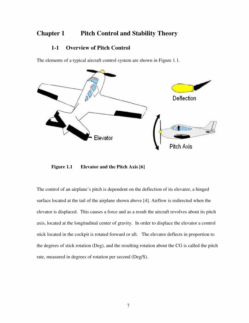
The elements of a typical aircraft control system are shown in Figure 1.1.
Figure 1.1 Elevator and the Pitch Axis [6]
The control of an airplane’s pitch is dependent on the deflection of its elevator, a hinged
surface located at the tail of the airplane shown above [4]. Airflow is redirected when the
elevator is displaced. This causes a force and as a result the aircraft revolves about its pitch
axis, located at the longitudinal center of gravity. In order to displace the elevator a control
stick located in the cockpit is rotated forward or aft. The elevator deflects in proportion to
the degrees of stick rotation (Deg), and the resulting rotation about the CG is called the pitch
rate, measured in degrees of rotation per second (Deg/S).

8
1-2 Aircraft Stability
Consider Figure 1.2. Note that the center of lift (CL) is a point that exists ¼ of the way back
from the leading edge of the wing. The center of gravity is point which moves based on the
weight distribution of an aircraft. Traditionally an aircraft is expected to be stable if the
center of gravity (CG) is located in front of the center of lift (CL). If the center of gravity
was located at the same place as the center of lift, the airplane would be neutrally stable. If
the CG was moved behind the center of lift, the aircraft would be unstable.
Figure 1.2 Airfoil, Center of Lift, and Center of Gravity Range
For the purposes of this work, it is important to understand two types of stability.
Static stability refers to the initial response of an aircraft after a perturbation from
equilibrium. An aircraft that tends to return to equilibrium after displacement exhibits a
restorative force called subsidence, and is statically stable. If the aircraft tends to depart
further from the equilibrium point after a disturbance, it exhibits divergence and is statically

9
unstable. If a disturbance does not result in the generation of either a restoring or departing
force, the aircraft is neutrally stable; this condition represents the boundary between stable
and unstable.
Dynamic stability is represented by the time history of motion of an aircraft after it has been
disturbed or a user input commands it from equilibrium. If an aircraft at equilibrium was
being displaced, the reduction of disturbance with time would imply a resistance to motion;
An aircraft with negative damping that was displaced from equilibrium would continue to
diverge from equilibrium. This departure could take the form of an exponential divergence
or growing oscillation. Any negatively damped aircraft would require constant pilot
attention and continuous correction, if it was flyable at all.
In cases of negatively damped aircraft, a closed loop control system can be employed to
provide restorative forces. This generally consists of an electromechanical system which
senses undesirable motion and responds by damping that motion.
10
Chapter 2 Plant Modeling
2-1 Elements of Pitch Behavior
The typical analysis of aircraft pitch behavior consists of the combination of two 2nd
order
linear transfer functions, describing short and long period stability characteristics called
modes. The combination of the two results in a 4th
order linear transfer function.
The long period mode, or phugoid, is a long term (>>short period) non-divergent oscillation
of an aircraft about the pitch axis. The phugoid is only present when the aircraft has positive
stability, (i.e. the CG is located in front of the center of lift in Figure 1.2). The period of the
phugoid is generally on the order of tens of seconds. If the aircraft is not positively stable
(CG behind the center of lift in Figure 1.2), the long period mode simplifies to a long term
divergence. This divergence can be ignored because the effects of the short period mode
(described below) are much greater.
The short period mode represents the immediate response to change, either in the form of
control inputs or atmospheric disturbances. The short period poles dominate the description
of short term flight behavior. Examining the short period poles reveal whether an aircraft is
stable or not, and allow the calculation of the DC gain ‘A’ so the pitch rate variation can be
found.
The long period oscillation was not taken into consideration in this analysis for two reasons.
First, the period of one oscillation (generally >10 seconds) is much longer than any response
of the short period mode, and second, the phugoid mode is only apparent for positive static

11
stability. If an aircraft has neutral or negative static stability the phugoid oscillation is not
present. As such, only the short period was of interest for the purposes of this work. As a
result of eliminating the long period mode, the description of flight was simplified to a
second order transfer function.
2-2 DATCOM Modeling
Modeling the pitch behavior of an aircraft required calculating a variety of ‘control
derivatives’. These control derivatives (Defined in Tables 2.1-2.3) are measures of how
forces and moments on an aircraft change as other parameters related to stability change. A
complete set of control derivates can be used to mathematically model flight behavior. The
common approach to determining control derivatives consists of a finite element analysis in
which the moments for small parts of the aircraft are summed. [5,7,11] Components that are
analyzed for longitudinal stability include the wing, fuselage, horizontal stabilizer, elevator,
and propulsion system. The contributions of each surface can be found through hand
calculation for a given operating condition and well-understood control surfaces. Although
hand calculation is a viable method, it is tedious and impractical for complex shapes. The
United States Air Force Stability and Control Data Compendium [5], commonly referred to
as DATCOM, performs the finite element analysis described, and provides a method for
modeling the behavior of an airframe in a computer simulation. An example of the
utilization of DATCOM can be found in Model-Based Design of a New Light-weight
Aircraft, [12].

12
The plant that I used for this comparative control evaluation was a Scorpio Miss 2 radio
controlled aircraft (Figure 0.1). The characteristics of this aircraft were modeled by
measuring all the physical characteristics (wing area, span, chord, length, width, weight, CG
location, etc), as well as the flight speed, density of air, and the force of gravity, and creating
a data file. DATCOM used the data file to calculate values for control derivatives.
DATCOM was used within Mathworks Simulink® and MatLab® to describe the system
plant. The input variables, model parameters, and outputs of DATCOM are defined in
Tables 2.1, 2.2, and 2.3.
Table 2.1 Input Variables
Symbol Description Unit
eδ Elevator Deflection Angle degrees (+/- 15 limit)
Uo Aircraft True Flight Speed m/s
Table 2.2 Model Parameters
Symbol Description Value and Unit
m Aircraft Mass 1.4 kg
S Wing Planform Area .255 m2
c Mean Aerodynamic Chord 0.18 m
b Wing Span 1.370 m
Iy Pitching moment of inertia .17 kg-m2
Czδe Coefficient of downforce with
respect to elevator angle
-.3565 unitless
Cmδe Coefficient of moment with respect -1.3265 unitless

13
to elevator angle
CLά Coefficient of lift with respect to
change in angle of attack
-.171 unitless
g Gravity 9.8 m/s2
rho Density of air at sea level 1.29 kg/m3
CDo Parasite Drag coefficient (CL=0) unitless
CLo Zero Lift Coefficient (α =0) unitless
CLα Lift Curve Slope 1/deg
CMq Coefficient of Moment from θ& 1/deg
CMα Coefficient of Moment from α 1/deg
CMά Coefficent of moment from ά 1/deg
Qo Dynamic Pressure = 1/2*rho*Uo^2 Pa
Table 2.3 Output
Symbol Description Value and Unit
θ Aircraft Pitch Angle degrees
q Pitch Rate degrees/sec
To populate the longitudinal equation of motion that will be described shortly, the moments
and forces acting upon the aircraft were calculated using the equations shown in Table 2.4,
using the methods described in Glide-Slope Control Design [8] and Derivation and
Definition of a Linear Aircraft Model [10].

14
Table 2.4 Calculated Longitudinal Forces and Moments
Symbol Equation
Zw -( CLα + CDo) * Qo * S/(m * Uo)
Mw CMα *(Qo*S*c/(Uo*Iy))
Mwd CMά * (c/(2 * Uo) * Qo * S * c/(Uo * Iy))
Mq CMq * c * Qo * S *c/(2 * Uo * Iy)
Zδe Czδe *Qo*S/m
Mδe Cmδe * Qo * S * c/Iy
Mά Uo*Mwd
Mα Uo*Mw
Zα Uo*Zw

15
2-3 Longitudinal Equation of Motion
The equation for short period motion in state space form is described by Equation 2.1. This
form can be used to find a symbolic second order transfer function.
BuAxx +=&
DuCxy +=
[ ]e
ee
oe
qo
o
uZMM
uZ
qMMuZMM
uZx δ
α
δαδ
δ
αααα
α ∆
++
∆
∆
++=
0/
/
/
1/
&&&
&
[ ]
∆
∆=
qy
α10
Equation 2.1 Short Period Motion Description [7,8,9,10]
)(
)(
s
sq
eδ∆∆
[8,9], represents the transfer function for change in pitch rate to change in elevator
angle. Solving for this transfer function using Cramer’s Rule yields Equation 2.2.
)()/(
1/
)/(
//
)(
)(
0
αααα
α
δαδααα
δα
δ
&&
&&
MMsuZMM
uZs
u
ZMMuZMM
uZuZs
s
sq
qo
o
o
eeo
eo
e
+−+−
−−
++−
−
=∆∆
Equation 2.2 Pitch Range Change for Elevator Deflection
Simplifying Equation 2.2 led to a more convenient representation of the plant as the second
order transfer function shown in Equation 2.3. This transfer function describes the flight
behavior of the open loop system. Finding the limit of this transfer function as s goes to zero
(as shown later) directly yields the DC gain ‘A’.

16
)/()/(
)//()/(
)(
)(2
0
αααα
αδδαδαδ
δ MuMZsuZMMs
uZMuZMsuZMM
s
sq
oqoq
oeeoee
e −+++−
−++=
∆
∆
&
&
Equation 2.3 Simplified Transfer Function
2-4 Varying Transfer Function as a Plant Model
The typical linear transfer function of an aircraft plant subscribes to the small perturbation
model: a single transfer function is assumed to deliver accurate results over a small range of
operation about a fixed point [11]. This has the potential to make the description of aircraft
motion inaccurate over a broad range. Rather than using a single transfer function for the
aircraft plant, a varying transfer function was implemented by solving the symbolic transfer
function of Equation 2.3 during MatLab and Simulink simulation at each time step (.001
seconds). The varying transfer function was recalculated by DATCOM, based on the values
of the system variables of Tables 2.1 and 2.2. This method had the potential to more
accurately describe a large range of motion than an individual fixed transfer function.
Since the transfer function was calculated at each time step, the stability characteristics
changed at each time step. A typical linear system with a known transfer function would
allow the stability characteristics to be calculated, and values for a control system would be
readily identifiable. Since the plant of this thesis changed with each time step, finding a set
of PD control parameters representing an optimal control system was not possible. Rather, it
was of the utmost importance to develop a robust control system over a broad range of CG
locations.

17
2-5 Controllability
In order to develop a representation of the plant, it was important to determine controllability.
Constructing a controllability matrix and proving that it was of full rank shows whether the
available inputs affect all modes of the system. Recall Equation 2.1, showing the state space
representation of the linear transfer function. Knowing that the plant was of second order
(n=2), a controllability matrix WC was constructed of the form shown in Equation 2.5, from
Equation 2.1. [13] Matrices A and B are found in Equation 2.1.
[ ]ABBWC = , where
++=
αααα
α
&&MMuZMM
uZA
qo
o
/
1/ and
+=
0/
/
uZMM
uZB
ee
oe
δαδ
δ
&
+++++
++
=))(()(/
/
0
0
2
u
ZMMMM
u
ZMM
u
ZuZMM
u
ZMM
u
ZZuZ
We
eq
oo
e
ee
o
e
e
o
e
oe
Cδα
δααα
αδ
δαδ
δαδ
δαδ
&
&
&
&
&
Equation 2.5 Controllability Matrix
Since the transfer function varied, it was not possible to determine if the WC was of full rank
for all possible values. Rather, controllability was found numerically only for the flight
speed, CG locations, and step inputs tested in this simulation.

18
Chapter 3 Plant Development and Open Loop Simulation
3-1 Open Loop Simulation Method and Objectives
The objectives of open loop simulation were to examine the behavior of the Plant when
subjected to step inputs at several CG locations, to determine the Pitch Rate Gain Variance as
the CG changed, to determine maximum gain variation, and to verify system controllability
using Equation 2.5.
3-2 Plant Development
With a longitudinal equation of motion determined and DATCOM available to populate it,
open loop analysis required the creation of a plant in a simulation environment. This analysis
used the SIMULINK ® graphics modeling and simulation feature of MATLAB ®. Figure
3.1 shows the form of the open loop system.
Figure 3.1 Open Loop System
The Input block in Figure 3.1 creates a signal corresponding to the deflection of the control
stick, as described in Section 1-1 as the user input. This Input signal is realized by the Servo
block. The Servo directly actuates the elevator based on the magnitude of the signal it
receives. In the open loop case, the Servo output is directly proportional to the Input signal.

19
The Servo block in Figure 3.1 represents an approximation of the servo shown in Figure 3.2,
which is a typical radio control accessory. The servo is capable of rotating its full range in
.12 seconds. The input signal is refreshed every 20 milliseconds.
Figure 3.2 Hitec-RCD HS-81MG Servo [16]
Figure 3.3 shows the workings of the Servo block from Figure 3.1. The Zero-Order Hold
refreshed the Input every 20mS. The gain of the Slew Rate determined the speed of the
servo, and the Integrator (Int) tracked the position of the servo and limited the output to +/-
15 degrees.
Figure 3.3 Servo Block
It is important to note that inclusion of the servo block in the simulation environment
represents a departure from the description of the system provided by Equation 2.3. The
servo was not included in the transfer function for two reasons. Firstly, the servo as
described in Figure 3.3 was nonlinear by virtue of being bounded, and all other simulation

20
was based on the assumption that the plant was linear. The servo simply limits the travel of
the elevator, creating nonlinearity at the extremes of elevator position. Secondly, the
response of the servo to inputs was more than an order of magnitude faster than the rest of
the system response. As a result, the behavior of the servo had a minimal effect on the
overall system, thus the servo was not included in the transfer function.
The Dynamic Transfer Function of Figure 3.1 is shown in detail in Figure 3.4,
followed by a flowchart describing its function in Figure 3.5.
Figure 3.4 Dynamic Transfer Function Block

21
Figure 3.5 Dynamic Transfer Function Flow Chart

22
The Dynamic Transfer Function worked by first loading initialization data corresponding to a
given CG into MATLAB memory. The initial flight speed and motor thrust were also input.
For each time step, the Dynamic Transfer Function first received the input Control In from
the Servo Output, as shown in Figure 3.1. The system calculations were performed in
radians/s, so the input signal was immediately scaled to convert from deg/s. The
initialization data and flight speed previously loaded were used by the Cma_in De, Cma_in
Mach, and Cmq_in De functions to determine values for each of them based on Control In, as
shown in the flowchart as “calculation of coefficients”. Next the embedded MATLAB
function PZthesis (shown as the large square in the middle) ran DATCOM within MatLab
and Simulink. PZthesis calculated the poles and zeros of a transfer function based on
DATCOM results. Those poles and zeros were passed to stvctf, which combined the poles
and zeroes found by PZthesis with the input signal, and calculated a response corresponding
to the pitch rate. That response was scaled again to convert back to deg/s from radians /s,
and is represented as the pitch rate, shown in the upper right hand corner of Figure 3.4.
Integrating the pitch rate signal resulted in a pitch angle signal, which was fed into the group
shown at the bottom of Figure 3.4. The group was initialized by inputting values for thrust,
drag, and airspeed. U0 was allowed to vary based on whether the pitch angle was positive or
negative. Simply, when the aircraft was climbing, the speed decreased, and when the aircraft
was descending, the speed increased. This representation in Simulink has been previously
utilized by Day et al. [8] as a method for describing variation in airspeed. The flight speed

23
varied with pitch angle, aircraft thrust, and speed-dependant drag. The change in flight speed
was calculated at every time step.
The open loop simulation was subjected to step inputs in 5 degree increments, from -15
degrees to +15 degrees, at each of five CG locations, entitled CG Location 28, 30, 32, 34,
and 36. These locations represent the distance rearward from the nose of the aircraft to the
location of the CG in centimeters, as shown in Figure 3.6. A larger number indicates a more
rearward CG.
Figure 3.6 CG Location
The step input corresponding to zero was not included in the plots. The CG as
recommended by the manufacturer of the Scorpio Miss 2 aircraft was 28 centimeters. The
flight speed used for uo was 10 meters/sec, representing the typical cruise speed of this
aircraft.
For each CG, the Open Loop DC Gain was calculated for each step input, averaged, and
appears graphically in section 3-3 Open Loop Simulation Results. The Open Loop DC Gain
was calculated using Equation 3.1 [14].
24
−+++−
−++
→=
)/()/(
)//()/(
0 2
0
αααα
αδδαδαδ
MuMZsuZMMs
uZMuZMsuZMM
s
LimDCGain
oqoq
oeeoee
&
&
Equation 3.1 Open Loop DC Gain
Once an average open loop DC gain was found for each CG location, the gain variation was
calculated as a percent increase from minimum to maximum open loop DC gain.
In addition, a plot of the poles and zeros was created for each CG location to examine pole-
zero movement with respect to CG location. It is important to note that the poles and zeros
shown represent their steady state values for a step input of +10 degrees of elevator
deflection. It was found during simulation that the poles and zeroes for each CG changed
minimally (less than 5%) over the range of step inputs, and could be represented as a fixed
value.
3-3 Open Loop Simulation Results
Figures 3.7-3.11 display the Open Loop outputs in response to the five step inputs as
described above and pole-zero plots, corresponding to the CG tested. The pole-zero plots
show two poles and one zero, corresponding to Equation 2.3. Note that the Pitch Rate
(Deg/s) scale grew larger with each successive plot, indicating that as the CG moved
rearward (increased numerically), the system gain increased.

25
Figure 3.7a Open Loop Output for CG 28
Figure 3.7b Open Loop Pole-Zero for CG 28

26
Figure 3.8a Open Loop Output for CG 30
Figure 3.8b Open Loop Pole-Zero for CG 30

27
Figure 3.9a Open Loop Output for CG 32
Figure 3.9b Open Loop Pole Zero for CG 32

28
Figure 3.10b Open Loop Output for CG 34
Figure 3.10b Open Loop Pole-Zero for CG 34

29
Figure 3.11a Open Loop Output for CG 36
Figure 3.11b Open Loop Pole-Zero for CG 36

30
Examining Figures 3.7-3.11 shows the degrading stability of the system as the CG moves
rearward. CG locations 28, 30, and 32(Figures 3.7 and 3.8) were stable, with poles and zeros
located in the left plane.
CG location 32 (Figure 3.9) was stable as well, but with a noticeable oscillation. This
oscillation was not the result of instability, but rather an artifact of the airspeed changing.
Note the top trace in Figure 3.9 had a period of oscillation of about 1.6 seconds. Note also
that the Pitch Rate appeared to have a steady state average value of about 220 degrees per
second. Every 1.6 seconds the simulation was completing a 360 degree rotation. This was
analogous to performing a loop. As the airspeed varied, the effectiveness of the elevator
varied, thus causing a change in Pitch Rate. CG locations 28 and 32 exhibited this behavior
as well, but the Pitch Rate was low enough that the variation was not as noticeable.
CG location 34 (Figure 3.10) was unstable, with a pole located barely in the right half plane.
The oscillations seen on each trace were again the result of changing airspeed. Note that
scale of the Pitch Rate was likely beyond the limits of the flight envelope. The system was
exponentially divergent.
CG location 36 (Figure 3.11) was clearly unstable, with a pole well into the right half plane.
The traces show a divergent system, with the scale of the Pitch Rate orders of magnitude
beyond the possible flight envelope.

31
Figure 3.12 shows a graph of the Open Loop DC Gain (calculated using Equation 3.1) with
respect to the CG as it varied from location 28 to 36. It is of interest to note that the Open
Loop DC Gain continues to increase as the CG moves rearward. Remember from above
discussion that the plant became unstable around CG location 34.
Figure 3.12 Open Loop DC Gain with Respect to CG
By examining the values of gain for CG locations 28 and 36 in Figure 3.12, Equation 3.2
calculated that CG 36 represented an increase in gain of 334% from CG 28.
%33428
)2836(=
−CG
CGCG
Equation 3.2 Open Loop Gain Percentage Increase

32
Additionally, the controllability of the transfer function was tested at each CG location. In
all test cases the system was calculated to be controllable, as the matrix of Equation 2.5
remained of full rank.
3-4 Open Loop Conclusions
The open loop Plant was subjected to an array of inputs at several CG locations as described
above. The plant was found to increase in gain and decrease in stability as the CG moved
rearward, as suspected. For the rearmost two CG locations, poles existed in the right half of
the pole-zero map, indicating that they were unstable.

33
Chapter 4 Control System Development and Simulation
4-1 Control System Objectives
The focus of this work was to design a robust control system that minimized Pitch Rate
Variance with respect to CG movement. The open loop simulation showed that the aircraft
chosen decreased in stability and increased in gain as the CG moved rearward. To correct
this behavior, a closed loop control system needed to be developed. Once created, the closed
loop control system was subjected to the same inputs and CG locations as the open loop
system, and compared to the open loop of Chapter 3. 20% Pitch Rate Variance over the CG
range was considered acceptable, as opposed to the 334% increase for the open loop system
shown in Equation 3.2.
4-2 PD Control Law
A proportional-derivative (PD) control law was specified to govern the Controller block of
Figure 4.1. In the case of this work, the steady-state value of the Pitch Rate Gain of Figure
1.2 was of little importance. Of utmost importance was the minimization of Gain Variance
as CG changed. If the Variance could be kept within specification (<20% over the CG
range), an integrating term (to make a PID) would be unnecessary. Eliminating an
integrating term was attractive from an implementation standpoint, as it allowed the
possibility for a very simple analog circuit to be used as a controller if desired.
A PD control is described by Equation 4.1 [14,15]. The control law accepts an error
signal )(tE , the subtraction of a feedback signal from the user input. The control law creates
an output intended to reduce the error signal to zero.

34
))(())(( tEdt
dKtEKOutput Dp +=
(where E(t) = pitch rate error signal)
Equation 4.1 PD Control Law Structure
The proportional term consists of ))(( tEK p from Equation 3.1, which multiplies the error
signal )(tE by the scalar pK . By increasing the value of pK , the response of the control
system can be tuned to react more quickly to system error. This increase in response
typically results in overshoot if pK is large, and steady-state oscillation if pK is too large.
To combat overshoot, the derivative term adds dt
dKD ( )(tE ) to the Kp, ( )(tE ). This results
in a control system that can rapidly respond to changes in error signal, but slows down as the
error signal approaches zero. Thus, overshoot is minimized without compromising rapid
response, ensuring a controlled approach to steady-state equilibrium.
In this case, the PD control was bounded by the fact that the elevator has limited deflection.
This resulted in a multimode controller, with extremal control while the elevator was fully
deflected, and PD control while the elevator was not fully deflected [11,12]. The system
changed from extremal control to PD local control based on the magnitude of the error signal
and the rate of change of the error signal.

35
4-3 Control System Structure
Figure 4.1 Control System Structure
Figure 4.1 displays the feedback control system structure. The desired Pitch Rate at Input
entered a summing junction from which the feedback signal of an Angular Rate Sensor was
subtracted. The resulting error signal was sent to the Controller to augment stability and
then control the plant. The plant was modeled as the Dynamic Transfer Function described
in Chapter 3 and accepted data from the Controller, calculating the system response with
each time step. The Angular Rate Sensor measured the Pitch Rate and returned it back to the
summing junction for comparison to the input.
Figure 4.2 shows the workings of the Controller block.
Figure 4.2 Controller

36
The Controller block was comprised of a PD control in series with the Servo block described
in Chapter 3, Section 1. By varying the values of P and D, different gains were selectable for
simulation.
Figure 4.3 shows the Angular Rate Sensor block.
Figure 4.3 Angular Rate Sensor
The Angular Rate Sensor measured the Pitch Rate from the Dynamic Transfer Function,
scaled the Pitch Rate signal by ¼, and fed the signal into a Zero-Order Hold. The Zero-
Order Hold delayed the signal by .0001 seconds, for the sole purpose of avoiding a Simulink
computation error at time 0.
4-4 Control System Implementation
Describing the control system mathematically required an analytic form. Equation 4.2 shows
the transfer function for a closed loop system of the type shown in Figure 4.1 [14].
)()()(1
)()(
sHsGsK
sGsKClosedLoop
+=
Equation 4.2 Closed Loop Control System Form

37
In Equation 4.2, the term K(s) represents the forward transfer function of the Controller and
G(s) the Dynamic Transfer Function, while H(s) represents the feedback transfer function of
the Angular Rate Sensor. For simulation purposes, a symbolic representation of the closed
loop transfer function was required, and was formulated from Equation 2.3. It appears in
Equation 4.3.
( )
)()/()/(
)//()/()(1
)/()/(
)//()/(
2
0
2
0
FMuMZsuZMMs
uZMuZMsuZMMDsP
MuMZsuZMMs
uZMuZMsuZMMDsP
ClosedLoop
oqoq
oeeoee
oqoq
oeeoee
−+++−
−++++
−+++−
−+++
=
αααα
αδδαδαδ
αααα
αδδαδαδ
&
&
&
&
Equation 4.3 Closed Loop Transfer Function
Note that the term K(s) from Equation 4.2 was been replaced in Equation 4.3 by (P+Ds),
representing a PD control system with proportional gain P and derivative gain D, and that the
feedback transfer function was a scalar F.
With a transfer function available from Equation 4.3, the closed loop gain of the system
could be calculated by taking the limit of the system as shown in Equation 4.4.
( )
−+++−
−++++
−+++−
−+++
→=
)()/()/(
)//()/()(1
)/()/(
)//()/(
0
2
0
2
0
FMuMZsuZMMs
uZMuZMsuZMMDsP
MuMZsuZMMs
uZMuZMsuZMMDsP
s
LimDCGain
oqoq
oeeoee
oqoq
oeeoee
αααα
αδδαδαδ
αααα
αδδαδαδ
&
&
&
&
Equation 4.4 Closed Loop DC Gain

38
4-5 Closed Loop Simulation Method and Objectives
The objectives of closed loop simulation were to examine the behavior of the control system
when subjected to a variety of inputs at several CG locations, to find parameters for a PD
control system that provided satisfactory results, to determine the Pitch Rate Gain Variance
as the CG changed in order to calculate a percentage increase in gain, and to verify system
controllability using Equation 2.5.
The closed loop simulation was subjected to the same inputs and CG variations as described
in Chapter 3, Section 2.
For each CG, the Closed Loop DC Gain was calculated for each step input, averaged, and
appears in section 4-5 Open Loop Simulation Results. The Closed Loop DC Gain was
calculated using Equation 4.4.
In addition, a pole-zero plot was created for each CG location using the same method as the
open loop system.
Prior to testing the control system the initial gain for the P term in the control system needed
to be determined. The Ziegler-Nichols Closed Loop Method [16,17] was used. The
derivative gain KD was initially set to zero. A critical gain KC was calculated, representing
the maximum proportional gain possible without steady-state oscillation. The critical gain
KC of 4.6 was found to cause an oscillatory response. Ziegler-Nichols requires an initial
proportional gain KP of KC/1.7. In this case, that yields a KP gain of 2.7. The KD term was

39
set to zero, and the system was subjected to the regime of inputs and CG locations. The
system was iteratively tuned to minimize DC Gain Variance, and the P gain was set at 2.9. It
is important to note that the KD term does not affect DC gain at steady state, so performing
iterative tuning with KD set to zero was appropriate.
In order to find the value of the Derivative gain KD, the proportional gain KP was temporarily
set above the critical gain KC, resulting in steady state oscillation. Ziegler-Nichols used the
period of oscillation to recommend a derivative gain KD of 0.5, which provided acceptable
performance.
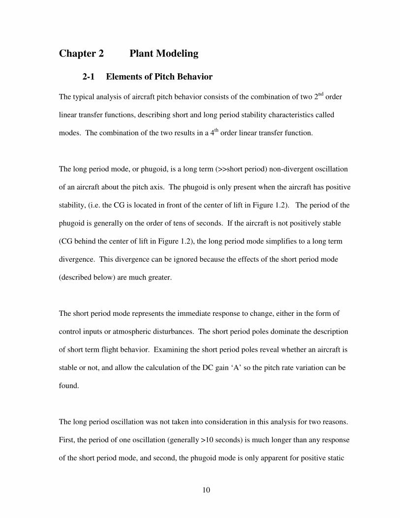
4-6 Closed Loop Simulation Results
Figures 4.4-4.8 display the Closed Loop outputs in response to step inputs, and pole-zero
plots corresponding to the CG tested. Each response graph shows the traces resulting from
step inputs of -15,-10,-5, 5,10, and 15 degrees for a given CG.

40
Figure 4.4a Closed Loop Output for CG 28
Figure 4.4b Closed Loop Pole-Zero for CG 28

41
Figure 4.5a Closed Loop Output for CG 30
Figure 4.5b Closed Loop Pole-Zero for CG 30

42
Figure 4.6a Closed Loop Output for CG 32
Figure 4.6b Closed Loop Pole-Zero for CG 32
43
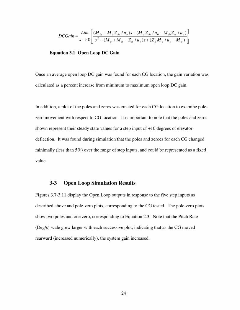
Figure 4.7a Closed Loop Output for CG 34
Figure 4.7b Closed Loop Pole-Zero for CG 34

44
Figure 4.8a Closed Loop Output for CG 36
Figure 4.8b Closed Loop Pole-Zero for CG 36

45
Examining Figures 4.4-4.8 shows the stability of the system as the CG moves rearward. The
pole-zero plots show that all CG locations were stable, with poles and zeros located in the
left plane. The plots look similar, but are not identical, as will be shown in Chapter 5.
Figure 4.9 shows a graph of the Closed Loop DC Gain (calculated using Equation 4.4) with
respect to the CG as it varied from location 28 to 36.
Figure 4.9 Closed Loop DC Gain with Respect to CG
By examining the values of gain for CG locations 28 and 36 in Figure 4.9, Equation 4.5
calculated that CG 36 represented an increase in gain of 8.5% from CG 28.
%5.828
)2836(=
−CG
CGCG
Equation 4.5 Closed Loop Gain Percentage Increase
46
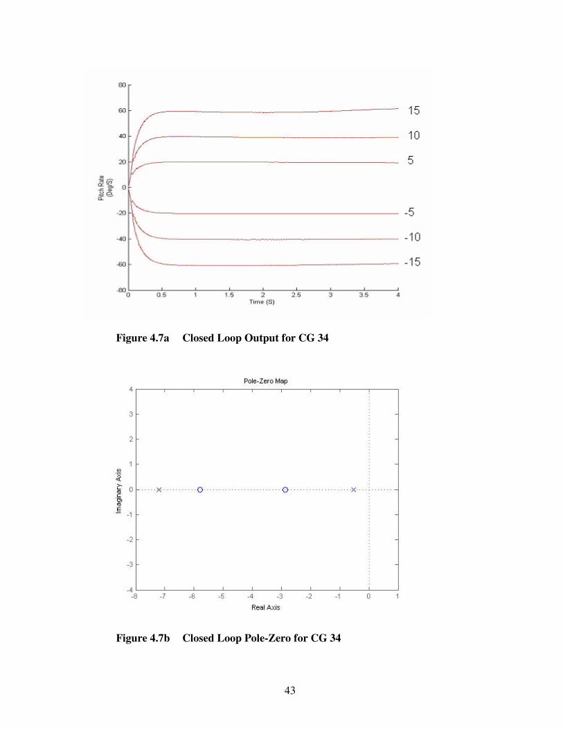
Additionally, the controllability of the transfer function was tested at each CG location. In
all test cases the system remained controllable, as the matrix of Equation 2.5 remained of full
rank.
4-6 Closed Loop Conclusions
The closed loop control system was subjected to an array of inputs at several CG locations.
Stability was examined and the closed loop system was found to be stable at all CG
locations. The DC gain ‘A’ was measured and the gain variance was shown graphically and
as a percent increase.

47
Chapter 5 Comparison of Open and Closed Loop
5-1 Open and Closed Loop Gain as a Function of the
Location of CG As seen by comparing Figures 3.12 and 4.9, and by reading sections 3-3 and 4-5, the closed
loop system limited the Pitch Rate Variance to 8.5%, as opposed to the open loop Pitch Rate
Variance of 334%, over the range of CGs tested. The closed loop system was well within the
desired performance parameter of less than 20% variation.
Figure 5.1 Open Loop and Closed Loop Gain ‘A’ Vs CG Movement

48
Examining Figure 5.1 shows the difference in Pitch Rate Variance as CG changes by
showing the open and closed loop gains. Note for that the CG recommended by the
manufacturer of 28, the gain was similar for both open and closed loop. As the CG moves
rearward (increases numerically on the X axis) the open loop gain increases rapidly, while
the closed loop gain increases only slightly. Even at the most unstable CG location (36), the
closed loop gain was similar in magnitude to the open loop gain when the open loop was at
the most stable position (28). This indicated that the closed loop control system robustly
controlled gain variation over the broad range of CGs tested.
5-2 Pole-Zero Plot Comparison
A complete set of pole-zero plots can be found for the open loop in section 3-3, and for the
closed loop in section 4-6. In the interest of observing the changing poles and zeros with
respect to CG, each of the open and closed loop plots have been combined into composite
open and closed loop plots, shown in Figures 5.2 and 5.3, with the CG listed next to each
pole or zero.
Figure 5.2 Open Loop Poles and Zero as CG Changes

49
Examining Figure 5.2 shows the behavior of the open loop poles and zero as the CG varies.
CG locations 28, 30, and 32 had complex poles located on a slight arc. CG location 34 had a
pole at about -3.2, and another just into the right half plane, indicating it was unstable. CG
location 36 has a pole at about -4.1, and another in the right half plane at about 1, indicating
it too was unstable. As the CG moved forward (decreased numerically), the system became
more stable, with poles moving from the right half plane into the left half plane. Somewhere
between CG 32 and 34, the poles collided on the real axis, formed complex roots, and moved
away from each other on the arc starting at about -1.5. The open loop numerator was not
largely affected by the change in CG, thus the locations of the zeros ranged from about -2.6
for CG 28 to -3 for CG 36.
The open loop plot (Figure 5.2) clearly shows the decay in stability as the CG moves
rearward.
Figure 5.3 Closed Loop Poles and Zeros as CG Changes
Figure 5.3 presents the pole-zero map for the closed loop system. The two poles for each CG
are both located on the real axis, indicating an overdamped system. The closed loop poles

50
moved very little with respect to CG movement. Note that the PD controller added a zero as
a result of the derivative term. Since the value of the P and D terms in the PD controller
were fixed, that zero never moved with respect to CG. The compensator zero was located at
about -5.5. Although it appeared as a single zero in the plot, the zero for each CG is located
in the same place. The set of zeros yielded by the plant were located from about -2.6 to -3,
and corresponded with the zeros of the open loop plot of Figure 5.2.
The closed loop plot (Figure 5.3) clearly showed that the poles and zeros move relatively
little with respect to CG movement, especially in comparison to the open loop of Figure 5.2.
This translated into a system that was stable, with similar stability characteristics for a broad
range of CG values.
It should be discussed that the varying transfer function demonstrated minimal changes in
pole-zero locations for a variety of step inputs. Figure 5.4 below shows the minimal
movement of the poles and zero for a complete set of open loop simulations at CG location
28. It was expected that pole-zero movement would be more significant. As a result of this
minimal movement, the poles and zeros in the plots were represented in the plots above as
single points, rather than a range of values.

51
Figure 5.4 Open Loop Pole-Zero Shift for CG 28
5-3 Response Comparison
The complete graphical results from the open loop and closed loop tests can be found in
sections 3.3 and 4.6, respectively. Examining the open and closed loop responses (Figures
5.5 and 5.6) for the rearmost CG (CG 36) showed that the closed loop control system was
capable of stabilizing the system at its most unstable location.

52
Figure 5.5 Open Loop Response at CG 36
Figure 5.6 Closed Loop Response at CG 36
The closed loop response of Figure 5.6 showed a smooth, overdamped response to a step
input that was free from overshoot or oscillation.

53
5-4 Controllability
Controllability was monitored continuously for all simulation trials by calculating the
controllability matrix of Equation 2.5 and determining its rank. At no point in any of the
simulations was the controllability matrix found to be of less than full rank, indicating that
the system was controllable for all simulation cases.
5-5 Comparison Conclusions
Having examined the open and closed loop systems with a variety of metrics, it was
concluded that the closed loop bounded PD control system exceeded the desired performance
criteria of minimizing Pitch Rate Variance to less than 20% and was a robust solution.
54
Chapter 6 Aircraft Flight Testing
6-1 Building the Model Airplane
A Scorpio Miss 2 aircraft of Figure 1.3 was assembled and outfitted with a microprocessor,
rate gyro, and additional the equipment described in Appendix A. A description of how the
electrical system was interconnected is available in Appendix B.
Machine code was written for the microprocessor in the Forth programming language to
implement the PD control system described in this work. That code and a description of its
operation are located in Appendix B. Onboard data storage was not available to record the
behavior of the aircraft, so all conclusions drawn from flight testing are strictly the result of
visual observation. The gain values found in simulation were implemented and tested in the
flying model.
6-2 Flight Testing Methods
The radio controlled aircraft was tested at the California Polytechnic State University
intramural sports fields and at the San Luis Obispo SLOFLYERS radio controlled flying
field located near Cuesta College, both located near San Luis Obispo, California.
The aircraft was launched from the ground with a fully stable center of gravity, with the
control system turned off by the transmitter. The aircraft was flown to a safe altitude that
allowed full recovery in the case of loss of control. This was estimated to be about 200 feet
above ground level. It was imperative to maintain a safe altitude while performing flight
testing. This allowed adequate time to return the aircraft to a stable state and recover control

55
if the control system exhibited undesirable behaviors, such as divergence or oscillations. If
altitude was not maintained, the risk of airframe destruction increased dramatically. The risk
to observers was also minimized by ensuring a large distance between spectators and the
aircraft.
To keep flight testing as safe as possible, takeoffs and landings were performed while fully
stable, and with the control system turned off. This minimized the chance of a problem with
the control system causing the aircraft to be uncontrollable while at low altitude or in
proximity to people.
After takeoff and once at testing altitude, a cruise speed of about 10 m/s was established by
setting the throttle to 50%. The control system was switched on using the transmitter, while
maintaining a fully stable CG. The response of the airplane was tested with smooth inputs to
verify that the system was functioning properly. Aggressive inputs were then employed to
test the response of the craft.
The CG of the airplane was varied in flight by means of a servo-controlled weight which
could be adjusted from the ground with the transmitter. The airplane stability was changed
by commanding a servo to shift the weight from front (stable) to back (unstable) in the
airplane during flight. The aircraft was tested over the range of CGs simulated in this work.
Unfortunately pictures of this mechanism are unavailable.

56
To prove that the control system was operating correctly, at the rearmost center of gravity the
control system was switched off to demonstrate the behavior of the unstable plant. This
resulted in a destabilization of the craft. It was possible to make corrective inputs but
controlled flight was not sustainable. The control system was then switched back on. This
resulted in a restabilization of the aircraft, allowing it to continue flying stably.
After flight testing the control system over the range of CG locations and observing behavior,
the CG was returned to the stable location, the control system was turned off, and the aircraft
was landed.
6-3 Flight Testing Results
Video of flight testing is included in the attached compact disc. General comments and
observations were as follows:
1. For flight within the accepted speed envelope the control system appeared
stable, free from oscillation or divergence.
2. Flight tests at the edges of the flight speed envelope resulted in unusual
behavior. If the aircraft was flown slowly the elevator lacked sufficient airflow (and
therefore authority) to fully control the aircraft. A curious result of this was a
tendency of the aircraft to pitch back into a stable but unusual attitude when the CG
location was at its rearmost. The aircraft flew with an extremely high angle of attack,

57
relying on the thrust of the motor to lift the aircraft, rather than the lift of the wing. A
stable descent resulted. By adding thrust or pitching the nose down, speed was
gained, and the aircraft would begin normal flight. This behavior was very
predictable and entertaining from a piloting perspective, and offered an unusual
benefit in that the aircraft could be flown extremely slowly with respect to horizontal.
This was done by attempting to hover the aircraft with the propeller. This behavior
was not possible without the aid of the control system.
If the aircraft was flown at full throttle with the CG rearward, and then nosed over
into a vertical dive, a small pitch oscillation developed. This was likely due to a
combination of aircraft instability and a proportional gain in the local control that was
slightly too large. Flight was controllable throughout the occurrence of oscillation,
and the oscillation subsided when the aircraft speed was reduced, either by reducing
power or pitching the nose upward.
For normal flight speeds and maneuvers, the control system provided stability
augmentation that was noticeable and functional. Without the introduction of
stability augmentation, the aircraft would not have been flyable at rearward CG
locations.
3. The control system implemented worked equally well when the aircraft was
inverted. This made flight more entertaining for the pilot.

58
Chapter 7 Summary and Conclusions
7.1 Summary of Work Performed
The major part of this thesis describes the development of open and closed loop computer
simulations utilizing a varying transfer function (using DATCOM simulation, MatLab, and
Simulink) to portray an aircraft in flight. An open loop system was developed and tested to
determine stability, controllability, and pitch rate gain variance with respect to CG
movement. The test results showed that an open loop system did not have adequate stability,
and excessive pitch rate gain variance.
A closed loop PD control system was developed in the simulation environment to provide
stability and minimize pitch rate gain variance. The closed loop control system was
compared against the open loop to prove that the closed loop system satisfactorily stabilized
the aircraft and minimized pitch rate gain variance.
As a result of the analysis, the control system simulation was used to implement a flying
model aircraft. Flight testing of this vehicle demonstrated that the closed loop control system
performed satisfactorily.
7.2 Areas for Further Study
Several areas of this work were considered for additional research and development. They
include the use of system identification, the implementation of more complex control
structures, and lastly, the use of onboard data acquisition for gain scheduling or dynamic
control.

59
System identification techniques would allow a more accurate description of the aircraft
throughout the flight regime. The simulation in this work relied on a DATCOM model for
data pertaining to flight behavior. Instrumenting and testing an aircraft in flight to describe
the plant could significantly improve the accuracy of a simulation.
The aircraft used in this work could be fitted with data acquisition equipment. In doing so, a
direct comparison between the simulation model and the actual flying model could be made.
Servo position data and gyro input data could be stored to allow post flight analysis. The
result of such a comparison would yield conclusions regarding the accuracy of conventional
modeling methods, and the advantages or validity of a varying transfer function in this
application. The time limitations on this thesis prevented the implementation of data storage
and analysis.
7.3 Closing Remarks
The work performed within this thesis represents my efforts to accurately analyze several
aspects of control design, computer modeling, simulation, implementation, and
documentation for one practical example.
Computer simulation results showed that the open loop control system exhibited
unacceptable pitch gain variance, and that the closed loop control system not only minimized
gain variance, but also stabilized the aircraft in all test cases. The controller was also

60
implemented in a Scorpio Miss 2 radio controlled aircraft using an on-board microprocessor.
Flight testing showed that performance was satisfactory.
This work represents my personal attempt to improve myself, to further my education, and to
provide a work for others who have similar interests. I am grateful to those who have
assisted me along the way, and it is my hope that this work reflects some of the excellence
that was bestowed upon my learning process by those helping hands and minds.
61
Cited References
[1] Hirth, R., Keas, P., Digital flight stabilization system for a model glider, California
State Polytechnic University, San Luis Obispo, CA (1994)
[2] Bosworth, J., Linearized Aerodynamic and Control Law Models of the X-29A
Airplane and Comparison with Flight Data, NASA Technical Memorandum 4356,
Dryden Research Facility (1992)
[3] Heffley, R., Jewell, W., Aircraft Handling Qualities Data, NASA CR-2144,
Technical Report 1004-1 (1972)
[4] Hobby-Lobby International, Inc., 2007 <www.hobby-lobby.com>.
[5] Finck, R.D., USAF (United States Air Force) Stability and Control DATCOM (Data
Compendium), McDonnel Douglas Aircraft Co. St. Louis MO, Accession
ADB072483 (1978).
[6] Raymer, D.P., Aircraft Design: A Conceptual Approach (American Institute of
Aeronautics and Astronautics, Reston, VA 1999) 481-523, 531-548.
[7] Ashley, H., Engineering Analysis of Flight Vehicles, (Addison-Wesley Pub. Co.,
Reading MA 1974).
[8] Day, K., Conti, J., Knobf, R. Lira, E., Reid, J., Ricca, E., Walter, R., Glide-Slope
Control Design, California State Polytechnic University, San Luis Obispo, CA
(2002)
[9] Milne-Thomson, L.M., Theoretical Aerodynamics, (Dover Publications Inc. Mineola
NY 1958)

62
[10] Duke, E., Antoniewicz, R., Krambeer, K., Derivation and Definition of a Linear
Aircraft Model, NASA Reference Publication 1207, Ames Research Center, Dryden
Flight Research Facility (1988)
[11] Raghavan, B., Anathkrishan, N., Small Perturbation Analysis of Airplane Dynamics
with Dynamic Stability Derivatives Redefined, AIAA Atmospheric Flight Mechanics
Conference, San Francisco CA (2005).
[12] Turevskiy, A., Gage, S., Buhr, C., Model-Based Design of a New Light-weight
Aircraft, The MathWorks, Inc. Natick, MA 01760, American Institute of Aeronautics
and Astronautics (20 August 2007)
[13] MacCarley, A., Controllability, EE513 Lecture Notes, Section 17 (2004)
[14] Nise, N.S., Control Systems Engineering, Fourth Edition, (John Wiley & Sons, Inc.,
New York, NY 2004)
[15] Nelson, R.C., Flight Stability and Automatic Control (WCB/McGraw Hill, Boston,
MA, 1998) 35-78, 96-130, 133-164, 271-274, 283-314, 324-335.
[16] Skogestad,S., Probably the best simple PID tuning rules in the world, Journal of
Process Control (July 3, 2001)
[17] Bennett, J., Bhasin, A., Grant, J., Lim, W., PID Tuning via Classical Methods,
Univeristy of Michigan, (October 16, 2007)
[18] MaxAmps RC, 2006 <www.maxamps.com/products.php?cat=28>
[19] Morelli, E. A., Airplane Dynamics, Modeling, and Controls, NASA Langley
Research Center, Hampton, VA (1997)

63
[20] Brandon, J.M., Foster, J.V., Recent Dynamic Measurements and Considerations for
Aerodynamic Modeling of Fighter Airplane Configurations, NASA Langley Research
Center, Hampton, VA (1998)
[21] Stengel. R.F., Toward Intelligent Flight Control, IEEE Transactions on Systems,
Man, and Cybernetics, 23 No. 6 (1993) 1699-1717
[22] Castle Creations, Inc., 2006 <www.castlecreations.com/>
[23] Futaba USA, 2007, <www.futaba-rc.com/radios/futk75.html>
[24] New Micros, Inc., 2007 <www.newmicros.com>
[25] Hitec RCD USA, 2007, <www.hitecrcd.com>

Appendix A
Equipment Description

65
The Scorpio Miss 2 as shown in Figure A.1 was used as the plant for the model aircraft
simulated in this work.
Figure A.1 Scorpio Miss 2 [4]
For the flight testing portion found in Chapter 6, the following additional equipment was
utilized.
The aircraft was powered by a Park 400 12 pole external-rotor brushless motor, as shown
in Figure A.2. It’s rated at 120W continuous output.The motor turned a 10X7 electric
propeller. The motor was controlled by a Castle Creations Phoenix-35 sensorless
brushless motor controller (Figure A.3).

66
Figure A.2 Park 400 External Rotor Motor [4]
Figure A.3 Castle Creations Phoenix-35 [22]
A MaxAmps 1500mAh 12 volt Lithium Polymer battery (Figure A.4) served as a ‘Power
Battery’, powering the motor and control systems. A similar 380mAh Lithium Polymer
battery, called the ‘Flight Battery’, provided a clean source for the microcontroller.
Figure A.4 MaxAmps Lithium Polymer Power Battery [18]
Control surface and variable CG actuation were controlled by Hitec-RCD HS-81MG
metal gear micro servos (Figure A.5).

67
Figure A.5 Hitec-RCD HS-81MG Servo [25]
A Futaba 9CHP transmitter (Figure A.6) was used to control the aircraft.
Figure A.6 Futaba 9CHP [23]
A Hitec-RCD Electron 6 channel FM receiver (Figure A.7) received the control signals
from the transmitter.

68
Figure A.7 Hitec-RCD Electron 6 Receiver [25]
A MinPod microcontroller implemented the desired control algorithms. The MinPod
used a 16 bit Motorola DSP56F803 processor operating at 80 megahertz. Programming
was done in the Forth-type IsoMax real-time language.
Figure A.8 MinPod Microcontroller [24]
An Analog Devices iMems ADXRS150 angular rate sensor was used by the MinPod for
sensing rotation.

69
Appendix B
Aircraft Systems and Software

70
Aircraft Electrical Overview
Figure B.1 displays the connections between the equipment onboard the radio control
model aircraft used for flight testing. The Power Battery provided 12 volts direct current
(VDC) to the Speed Controller. The Speed Controller had an onboard voltage regulator
which powers the Receiver, the CG servo, and the Rudder Servo at 5VDC. The Receiver
sent commands to the Speed Controller, which synthesized a 3 phase AC output to the
Motor, to the CG Servo and Rudder Servo. The Receiver also sent two signals to the
Microcontroller: an elevator rate command and a three mode gain selection input. The
gain selection input facilitated the testing of multiple control system gains, and allowed
the control system to be adjusted and turned on or off remotely while in flight. The
elevator rate command was input to the control system for two positions of the gain
selection input, and was passed straight through to the Elevator Servo when the gain
selection input had turned the control system off. When the gain selection input
commanded the control system to operate, the Microcontroller accepted pitch rate
information from the Gyro Sensor and the elevator rate command, and performed control
system calculations. Commands to the Elevator Servo were subsequently output to
command the aircraft to attain the pitch rate desired. The Microcontroller, Elevator
Servo, and Gyro Sensor all received power from the Flight Battery, rather than from the
Receiver, with which they share a common ground. This ensured a power source for the
Microcontroller that was free from noise.

71
Figure B.1 Components of control system on model aircraft

72
Aircraft Software Overview
The New Micros microcontroller was programmed using the Forth-based Iso-Max
language, and installed using a terminal emulator. The full content of programmed code
is shown below, with an explanation of operation preceding it.
Variables were defined to accept gyro, servo, and gain selection inputs, as well as a servo
output, and internal variables.
The GETSERVO command was interrupt driven to check the servo input pin of the
microcontroller to determine the desired user input.
The GYRO command polled an Analog to Digital (A/D) input pin on the microcontroller
every 2.5 milliseconds (ms). The input from the A/D was sampled, and IIR filtered to
provide a noise-free gyro sensor pitch rate input.
Next, the SETSERVO command created a desired user pitch rate output. The value
found with GETSERVO was compared to the admissible range of input values for proper
operation. If the value was found to be outside the acceptable range the servo output was
defaulted to a neutral position. This feature functioned as a failsafe. If the transmitter
failed on the ground, or interference prevented the signal from reaching the receiver, the
aircraft would default to a neutral gliding attitude.
73
The CONTROL command polled the interrupt driven gain selection input to determine
whether a control system was active or not, and which one. When the control system was
activated, the CONTROL command determined which control system (PD or multimode)
to implement and created an elevator output command to the servo that represented the
desired output. If the control system was not activated, the CONTROL COMMAND
simply passed the value of SETSERVO to the elevator, circumventing the control system.
The elevator output command from either the multimode controller or from the passed
through value of SETSERVO was created every 20 ms. This frequency complied with
the industry standard for hobby servos.
The software was designed to run all commands every 2.5 ms. The interrupt driven
commands functioned in response to inputs from the Receiver every 20 ms, but all other
operations functioned with each cycle.
BEGIN MINPOD CODE
SCRUB
DECIMAL
VARIABLE SERVOINPUT EEWORD
VARIABLE CHKSRV EEWORD
VARIABLE DATA EEWORD
VARIABLE DATA0 EEWORD
VARIABLE DATA1 EEWORD
VARIABLE DATA2 EEWORD
VARIABLE DATA3 EEWORD
VARIABLE DATA4 EEWORD
VARIABLE DATA5 EEWORD
VARIABLE DATA6 EEWORD
VARIABLE DATA7 EEWORD
VARIABLE DATA8 EEWORD
VARIABLE DATA9 EEWORD
VARIABLE DATA10 EEWORD
VARIABLE DATA11 EEWORD
VARIABLE DATA12 EEWORD
VARIABLE DATA13 EEWORD

74
VARIABLE DATA14 EEWORD
VARIABLE DATA15 EEWORD
VARIABLE DATA16 EEWORD
VARIABLE DATA17 EEWORD
VARIABLE DATA18 EEWORD
VARIABLE DATA19 EEWORD
VARIABLE DATA20 EEWORD
VARIABLE DATACALC EEWORD
VARIABLE DATATEST EEWORD
VARIABLE DATAFLIP EEWORD
VARIABLE DTERM EEWORD
VARIABLE DTERM2 EEWORD
VARIABLE ERR EEWORD
VARIABLE ERR1 EEWORD
VARIABLE CON EEWORD
VARIABLE CONOUT EEWORD
: GETSERVO ( -- n )
TA1 CHK-PWM-IN
DUP
IF
DUP 500 U<
IF
DROP
ELSE
DUP
CHKSRV !
SERVOINPUT !
THEN
TA1 SET-PWM-IN
ELSE
DROP
0 CHKSRV !
THEN
; EEWORD
: GYRO ( -- n)
DATA9 @
DATA15 @
DATA16 !
DATA14 @
DATA15 !
DATA13 @
DATA14 !
DATA12 @
DATA13 !
DATA11 @
DATA12 !
DATA10 @
DATA11 !
DATA9 @
DATA10 !
DATA8 @
DATA9 !
DATA7 @
DATA8 !

75
DATA6 @
DATA7 !
DATA5 @
DATA6 !
DATA4 @
DATA5 !
DATA3 @
DATA4 !
DATA2 @
DATA3 !
DATA1 @
DATA2 !
DATA0 @
DATA1 !
ADC0 ANALOGIN 16 /
DATA0 !
DATA0 @ 2840 +
DATA0 !
DATA0 @
DATACALC !
DATA1 @ 3 / DATACALC @ +
DATACALC !
DATA2 @ 4 / DATACALC @ +
DATACALC !
DATA3 @ 5 / DATACALC @ +
DATACALC !
DATA4 @ 6 / DATACALC @ +
DATACALC !
DATA5 @ 7 / DATACALC @ +
DATACALC !
DATA6 @ 8 / DATACALC @ +
DATACALC !
DATA7 @ 9 / DATACALC @ +
DATACALC !
DATA8 @ 10 / DATACALC @ +
DATACALC !
DATA9 @ 11 / DATACALC @ +
DATACALC !
DATA10 @ 12 / DATACALC @ +
DATACALC !
DATA11 @ 13 / DATACALC @ +
DATACALC !
DATA12 @ 14 / DATACALC @ +
DATACALC !
DATA13 @ 15 / DATACALC @ +
DATACALC !
DATA14 @ 16 / DATACALC @ +
DATACALC !
DATA15 @ 17 / DATACALC @ +
DATACALC !
DATA16 @ 18 / DATACALC @ +
DATACALC !
DATACALC @ 3 /
DATACALC !
DATACALC @ 10 +
DATA !

76
; EEWORD
: SETSERVO ( n -- )
IF
TA2 CHK-PWM-IN
3000 SWAP U<
IF
TA2 SET-PWM-IN
CONOUT @ 2500 U<
IF
3840
TA0 PWM-OUT
THEN
CONOUT @ 5000 SWAP U<
IF
3840
TA0 PWM-OUT
ELSE
CONOUT @
TA0 PWM-OUT
THEN
ELSE
TA2 SET-PWM-IN
SERVOINPUT @ 2200 U<
IF
3840
TA0 PWM-OUT
THEN
SERVOINPUT @ 5200 SWAP U<
IF
3840
TA0 PWM-OUT
ELSE
SERVOINPUT @
TA0 PWM-OUT
THEN
THEN
THEN
; EEWORD
: CONTROL
7670 DATA0 @ -
DATAFLIP !
SERVOINPUT @ DATAFLIP @ -
ERR1 !
ERR1 @ 3840 +
ERR1 !
DATA20 @ DATA1 @ -
DTERM !
DTERM @ 4 *
DTERM2 !
ERR1 @ DTERM @ +
CON !
3200 CON @ SWAP U<
IF
2800

77
CONOUT !
ELSE
ERR1 @ 3840 -
ERR !
ERR @ 3 *
ERR !
ERR @ 3840 +
ERR !
ERR @ DTERM @ +
CONOUT !
THEN
CONOUT @ 4800 SWAP U<
IF
4800
CONOUT !
THEN
CONOUT @ 2800 U<
IF
2800
CONOUT !
THEN
CON @ 4400 SWAP U<
IF
4800
CONOUT !
THEN
; EEWORD
: INIT
TA2 ACTIVE-HIGH
TA2 SET-PWM-IN
TA1 ACTIVE-HIGH
TA1 SET-PWM-IN
TA0 ACTIVE-HIGH
65534 TA0 PWM-PERIOD
3840 SERVOINPUT !
3840 DATA0 !
3840 DATA1 !
3840 DATA2 !
3840 DATA3 !
3840 DATA4 !
3840 DATA5 !
3840 DATA6 !
3840 DATA7 !
3840 DATA8 !
3840 DATA9 !
3840 DATA10 !
3840 DATA11 !
3840 DATA12 !
3840 DATA13 !
3840 DATA14 !
3840 DATA15 !
3840 DATA16 !
3840 DATA17 !
3840 DATA18 !
3840 DATA19 !

78
3840 DATA20 !
3840 DATAFLIP !
3840 DATACALC !
0 CHKSRV !
0 DTERM !
0 DTERM2 !
3840 ERR !
3840 ERR1 !
3840 CONOUT !
3840 CON !
3840 DATA !
; EEWORD
: RUN
GETSERVO
GYRO
CONTROL
CHKSRV @ SETSERVO
; EEWORD
: MAIN
INIT
RUN
EVERY 20000 CYCLES SCHEDULE-RUNS RUN
; EEWORD
AUTOSTART MAIN
SAVE-RAM
END MINPOD CODE