control of quadrotor using deep neural network
TRANSCRIPT

Control of Quadrotor using Deep NeuralNetwork
A thesis submitted in fulfilment of the requirements
for the degree of Master of Science by Research
by
Pratyush Varshney
under the guidance of
Dr. Indranil Saha
Department of Computer Science and Engineering
INDIAN INSTITUTE OF TECHNOLOGY KANPUR
January 2020


Abstract
Name of the student: Pratyush Varshney Roll No: 16211402
Degree for which submitted: M.S. (By Research)
Department: Computer Science and Engineering
Thesis title: Control of Quadrotor using Deep Neural Network
Thesis supervisor: Dr. Indranil Saha
Month and year of thesis submission: January 2020
Synthesis of a feedback controller for nonlinear dynamical systems like a quadrotor requires
to deal with the trade-off between performance and online computation requirement of
the controller. Model predictive controllers (MPC) provide excellent control performance,
but at the cost of high online computation. In this thesis, we present our experience in
approximating the behavior of an MPC for a quadrotor with a feed-forward neural network.
To facilitate the collection of training data, we create a faithful model of the quadrotor
and use Gazebo simulator to collect sufficient training data. The deep neural network
(DNN) controller learned from the training data has been tested on various trajectories to
compare its performance with a model-predictive controller. Our experimental results show
that our DNN controller can provide almost similar trajectory tracking performance at a
lower control computation cost, which helps in increasing the flight time of the quadrotor.
Moreover, the hardware requirement for our DNN controller is significantly less than that
for the MPC controller. Thus, the use of DNN based controller also helps in reducing the
overall price of a quadrotor.

Acknowledgements
The work presented in the thesis was done under the guidance of Dr. Indranil Saha. I
would like to thank him for his guidance and constant motivation throughout the course
of my research. It was a wonderful experience working with him. He was a source of
optimism at times when I was frustrated by constant failures in my attempts. At such
times, he chose to spend a great deal of his valuable time to encourage me and to help me
learn.
I would like to acknowledge my collaborator Gajendra Nagar for helping me in the ex-
perimental setup. I would like to acknowledge the constant support of Suman Varshney
and Peeyush Varshney, my mother and brother. I thank Parishkrati, my sister for
always being an inspiration to work hard.
Last but not the least, I would like to thank Neetika for being an integral part of my life
and helping me see the good in life.
This work was supported by SERB Early Career Research Award ECR/2016/000474.
Pratyush Varshney
ii

Contents
Abstract i
Acknowledgements ii
Contents iii
Publication v
List of Figures v
List of Tables vii
Abbreviations viii
Symbols ix
1 Introduction 1
1.1 Introduction . . . . . . . . . . . . . . . . . . . . . . . . . . . . . . . . . . . . 1
1.1.1 Related Work . . . . . . . . . . . . . . . . . . . . . . . . . . . . . . . 2
2 Problem 4
2.1 Preliminaries . . . . . . . . . . . . . . . . . . . . . . . . . . . . . . . . . . . 4
2.1.1 Euler Angles . . . . . . . . . . . . . . . . . . . . . . . . . . . . . . . 4
2.1.2 Quadrotor Dynamics . . . . . . . . . . . . . . . . . . . . . . . . . . . 6
2.1.3 Quadrotor State-Space Model . . . . . . . . . . . . . . . . . . . . . . 8
2.1.4 Flight Stack Architecture . . . . . . . . . . . . . . . . . . . . . . . . 9
2.1.5 High Level Controller . . . . . . . . . . . . . . . . . . . . . . . . . . 9
2.1.5.1 Proportional-Integral-Derivative Controller . . . . . . . . . 10
2.1.5.2 Model Predictive Controller (MPC) . . . . . . . . . . . . . 10
2.1.6 Neural Networks . . . . . . . . . . . . . . . . . . . . . . . . . . . . . 11
2.2 Problem Description . . . . . . . . . . . . . . . . . . . . . . . . . . . . . . . 12
3 Methodology 13
iii

Contents iv
3.1 Simulation Model of Quadrotor . . . . . . . . . . . . . . . . . . . . . . . . . 13
3.2 Learn MPC Controller using Supervised Learning . . . . . . . . . . . . . . . 15
4 Experiment Results 17
4.1 Experimental Setup . . . . . . . . . . . . . . . . . . . . . . . . . . . . . . . 17
4.2 System Identification and Simulation Modelling . . . . . . . . . . . . . . . . 18
4.3 Approximating MPC using DNN . . . . . . . . . . . . . . . . . . . . . . . . 19
4.4 Comparison of MPC and DNN controllers . . . . . . . . . . . . . . . . . . . 21
4.4.1 Trajectory Tracking . . . . . . . . . . . . . . . . . . . . . . . . . . . 21
4.4.2 State cost . . . . . . . . . . . . . . . . . . . . . . . . . . . . . . . . . 23
4.4.3 Control Cost . . . . . . . . . . . . . . . . . . . . . . . . . . . . . . . 23
4.4.4 Flight Time . . . . . . . . . . . . . . . . . . . . . . . . . . . . . . . . 24
4.4.5 Computational Requirement . . . . . . . . . . . . . . . . . . . . . . 25
4.5 Generalization of DNN controller . . . . . . . . . . . . . . . . . . . . . . . . 25
4.5.1 Evaluation on f450 . . . . . . . . . . . . . . . . . . . . . . . . . . . . 26
4.5.1.1 Generating Controller independent of Mass . . . . . . . . . 26
4.5.2 Evaluation on Firefly . . . . . . . . . . . . . . . . . . . . . . . . . . . 28
5 Conclusion 29
5.1 Contribution . . . . . . . . . . . . . . . . . . . . . . . . . . . . . . . . . . . 29
5.2 Future Work . . . . . . . . . . . . . . . . . . . . . . . . . . . . . . . . . . . 30
5.2.1 Evaluating the trade-off between the number of layers and performance 30
5.2.2 Reinforcement Learning . . . . . . . . . . . . . . . . . . . . . . . . . 30
5.2.3 Robustness of the Neural Network based controller . . . . . . . . . . 30
Bibliography 32

Publication
Pratyush Varshney, Gajendra Nagar, Indranil Saha. DeepControl: Energy-Efficient
Control of a Quadrotor using a Deep Neural Network. In Proceedings of the IEEE/RSJ
International Conference on Intelligent Robots and Systems (IROS 2019). IEEE,
Macau, China, November 4-8, 2019.
v

List of Figures
2.1 Euler angles in quadrotor body frame . . . . . . . . . . . . . . . . . . . . . 5
2.2 Direction of the propellers of quadrotor. . . . . . . . . . . . . . . . . . . . . 6
2.3 Controller architecture of an autopilot. . . . . . . . . . . . . . . . . . . . . . 9
4.1 f450 Quadrotor . . . . . . . . . . . . . . . . . . . . . . . . . . . . . . . . . . 17
4.2 Block diagram of the experimental setup for DeepControl. The Ground Sta-tion sends the reference trajectory to the high-level DNN Controller runningon-board in the quadrotor. The low-level attitude controller maintains thedesired orientation. The VICON system provides localization feedback forthe controller. . . . . . . . . . . . . . . . . . . . . . . . . . . . . . . . . . . . 18
4.3 Orientation tracking of the Real Flame-Wheel 450 quadrotor. The blueline represents the orientation of the quadrotor and red line represents thecommanded angles. . . . . . . . . . . . . . . . . . . . . . . . . . . . . . . . . 19
4.4 Orientation tracking of the simulator model of Flame-Wheel 450 quadro-tor. The blue line represents the orientation of the quadrotor and red linerepresents the commanded angles. . . . . . . . . . . . . . . . . . . . . . . . 20
4.5 Flying Arena . . . . . . . . . . . . . . . . . . . . . . . . . . . . . . . . . . . 20
4.6 Comparison of performance between MPC and DNN controllers for trajec-tory of 1m× 1m square for real-world f450 quadrotor. . . . . . . . . . . . . 22
4.7 Comparison of performance between MPC and DNN controllers for ∞-shaped trajectory for real-world f450 quadrotor. . . . . . . . . . . . . . . . . 22
4.8 Comparison of performance between MPC and DNN controller for stepresponse for real-world f450 quadrotor. . . . . . . . . . . . . . . . . . . . . . 22
4.9 Trajectory tracking error for MPC and DNN controller for ∞ shaped tra-jectory . . . . . . . . . . . . . . . . . . . . . . . . . . . . . . . . . . . . . . 23
4.10 Comparison of Control signals generated by MPC and DNN for ∞ shapedtrajectory and aggressive trajectory (step input). . . . . . . . . . . . . . . 24
4.11 Comparison of performance between MPC and DNN controller for f450quadrotor. . . . . . . . . . . . . . . . . . . . . . . . . . . . . . . . . . . . . . 28
4.12 Comparison of performance between MPC and DNN controller for infinityshaped trajectory for firefly hexarotor. . . . . . . . . . . . . . . . . . . . . . 28
vi

List of Tables
4.1 Comparison of Trajectory cost between MPC and DNN Controller for real-world f450. . . . . . . . . . . . . . . . . . . . . . . . . . . . . . . . . . . . . 24
4.2 Comparison of Flight time between MPC and DNN Controller for real-worldf450 . . . . . . . . . . . . . . . . . . . . . . . . . . . . . . . . . . . . . . . . 25
4.3 Comparison of CPU usage on a single core ARM Cortex A7 processor. . . . 25
4.4 Comparison of Trajectory cost between MPC and DNN Controller for f450with different mass. The DNN controller is trained with the mass of 1.45 Kg. 27
vii

Abbreviations
UAV Unmanned Aerial Vehicle
MPC Model Predictive Control
PID Proportional Integral Derivative
DNN Deep Neural Network
ROS Robot Operating System
F450 Flamewheel 450
GCS Ground Control Station
ESC Electronic Speed Controllers
viii

Symbols
t time
φ roll angle
θ pitch angle
ψ yaw angle
p position
ζ euler angles
τ thrust
ω angular velocity
ψ yaw rate
st state at time t
S state-space
U control-space
E error space
CT rotor thrust constant
CM rotor moment constant
Ti torque
Fi Force
ix

Dedicated to the memory of my Mother and Father. . .
x

Chapter 1
Introduction
1.1 Introduction
Autonomous dynamical systems like quadrotors rely on the efficacy of the feedback con-
trollers for their correct operations in uncertain environments. Synthesizing feedback
controllers for nonlinear dynamical systems poses tremendous challenges to the control
engineers as they need to deal with the trade-off between the performance of the con-
troller and the amount of online computation required for their efficient operation. For
example, Proportional Integral Derivative (PID) controller [78] has a simple structure
leading to very low online computation overhead. But the performance of PID controllers
for complex nonlinear systems is often not satisfactory. On the other hand, a Model Pre-
dictive Controller (MPC) [24] can provide excellent performance at the cost of a high
online computation overhead even for a system with linear dynamics. The optimization
problems solved in the MPC become further complicated when the system is nonlinear [8].
Although there exist optimization techniques like Sequential Convex Optimization [68]
that can solve the nonlinear optimization problems, they suffer from the lack of scalability
for complex systems with a large number of state variables.
To use an MPC as an on-board controller for a quadrotor, we need to mount a high-
performance computer on the quadrotor. However, the high energy requirement of the
MPC control computation on the onboard processor reduces the flight time. Adding extra
battery may help in increasing the flight time, but reduces the payload capacity. Em-
ploying the explicit MPC [77, 13] strategy could help in reducing the online computation.
However, as observed in [16], the computation time to synthesize an explicit controller
grows exponentially both in the number of time steps and the size of the state and input
1

Chapter 1. Introduction 2
vectors, thus making explicit MPC not suitable for a high-dimensional nonlinear dynamical
system like quadrotor.
In this thesis, we explore the possibility of synthesizing a feedback controller for a quadrotor
in the form of a neural network. We employ supervised learning [62] where we generate
training data capturing the state-control mapping from the execution of a model predictive
controller. However, the generation of training data by flying a quadrotor is tedious as the
battery of the quadrotor needs to be charged for several times in the process of generating
the training data. To alleviate this problem, we create a faithful model of the quadrotor
that can be used for simulation on the Gazebo Simulator [23] to generate the required
training data.
1.1.1 Related Work
Various control mechanisms have been introduced for quadrotors, for example, sliding-
mode control [80], feedback linearization [79], H∞ robust control [57], adaptive control [52],
and minimum snap trajectory-based control [48]. All these control mechanisms assume the
availability of a faithful mathematical model of the quadrotor. To address this limitation,
Bansal et al. [11] has recently proposed a mechanism to model the dynamics of a quadrotor
using a neural network and showed how this neural network-based model can be used for
control computation. Li et al. [43] have used a DNN to generate a feasible reference
trajectory from a user given the desired trajectory for a quadrotor. Sanchez et al. [65]
have shown that deep neural networks can be used as controllers for spacecraft landing.
Their results are restricted to simulations with the assumption that they have access to
perfect states without any sensor errors.
There has been some recent work on synthesizing neural network-based feedback con-
trollers for dynamical systems. Recent work has shown that Reinforcement Learning [74]
based policy search can be successfully used to synthesize a controller for a nonlinear dy-
namical system like quadrotor [36]. The authors have used Actor-Critic Algorithm [71]
to synthesize the controller. Zhang et al. [81] proposed a methodology to train a neural
network through a policy search guided by the data generated from an MPC under full
state observations. However, the time required for such a policy search is large as com-
pared to that of supervised learning-based algorithms. Recently, Chen et al. [19] proposed
a methodology for approximating an MPC using a Neural Network. The authors show
that using Dykstra’s projection they are able to reduce the policy search space. However,
their approach is restricted to linear systems.

Chapter 1. Introduction 3
The contribution of the thesis is as follows:
• Synthesizing a Deep Neural Network based controller from a Model Predictive Con-
trol.
• Creating a faithful model of the real-world quadrotor in the simulation to generate
training data.
• Deployment of learned DNN controller on the real-world quadrotor.
• Evaluation of the Deep Neural Network based controller and MPC in the real-world
scenario, on various matrices like: trajectory error, flight time, processor usage.

Chapter 2
Problem
2.1 Preliminaries
The quadrotor is an Unmanned Aerial Vehicle (UAV) which is highly maneuverable. It
consists of four rotors mounted on a frame. The motion of the quadrotor can be divided
into two parts: (i) Translational motion (ii) Rotational motion. The rotational motion is
responsible for the change of orientation of the quadrotor. The translational motion for
quadrotor can be seen as a set of changes of orientation of the quadrotor. This means that
to change the position of the quadrotor, the vehicle must go through the set of changes in
its orientation.
2.1.1 Euler Angles
The 3-dimensional motion of the quadrotor is described by two frame of reference:
(i). inertial frame : attached to the Earth
(ii). body frame: attached to the body of the quadrotor
There are some quantities that are measured in inertial frame like position and velocity,
while some quantities like angular velocities and attitude are measured in body frame of
the quadrotor. Therefore, a transformation matrix is required to convert the measured
quantities from one frame to another.
4

Chapter 2. Problem 5
Figure 2.1: Euler angles in quadrotor body frame
This is transformation matrix is obtained using the Euler angles [21] that describe the
orientation of a frame relative to another frame. The frame transformation is done by se-
quentially rotating the three axes like ZXZ, XYX etc. The transformation is parameterized
by three angles.
(i). yaw angle (ψ): the angle of rotation around z-axis
(ii). pitch angle (θ): the angle of rotation around y-axis
(iii). yaw angle (φ): the angle of rotation around x-axis
The rotation matrices [12] are defined as:
Rx(φ) =
1 0 0
0 c(φ) −s(φ)
0 s(φ) c(φ)
Ry(θ) =
c(θ) 0 s(θ)
0 1 0
−s(θ) 0 c(θ)
Rz(ψ) =
c(ψ) −s(ψ) 0
s(ψ) c(ψ) 0
0 0 1
where c(x) = cos(x), s(x) = sin(x). The rotation from body frame to inertial matrix is
defined by
Rzyx(φ, θ, ψ) = Rz(ψ) ·Ry(θ) ·Rx(ψ) (2.1)
=
c(θ)c(φ) s(φ)s(θ)c(ψ)− c(φ)s(φ) c(φ)s(θ)c(ψ) + s(φ)s(ψ)
c(θ)s(ψ) s(φ)s(θ)s(ψ) + c(φ)c(ψ) c(φ)s(θ)s(ψ)− s(φ)c(ψ)
−s(θ) s(φ)c(θ) c(φ)c(θ)
(2.2)

Chapter 2. Problem 6
2.1.2 Quadrotor Dynamics
The following quantities define the quadrotor
• m : mass of the quadrotor
• l: arm length of quadrotor.
• Fi: force due to rotor i
• Ti: torque due to ith rotor
• Tφ, Tθ, Tψ: rolling, pitching, yawing torque
• Ωi: angular velocity of ith rotor
The structure of quadrotor consists of four rotor blades placed equidistant from the center.
The spinning rotors create thrust and moments that is responsible for the movement of
quadrotor in 3-dimensional space. The four rotors have their propellers arranged such
that the diagonal propellers spin in the same direction i.e. clockwise/anti-clockwise. The
adjacent propellers spin in the different direction to each other as shown in Fig. 2.2
Figure 2.2: Direction of the propellers of quadrotor.
The diagonally opposite propellers spin in the same direction while adjacent propellersspin in the opposite direction. [63]
These propellers generate force in the upward direction that generates the thrust for the
quadrotor. The translation and rotational motion of the quadrotor is achieved by adjusting
the rotor speeds.
Chapter 2. Problem 7
(i). z-axis: For motion along z-axis, all the rotors have equal angular speed. Increas-
ing/decreasing the angular speed results in increase/decrease in altitude. Total force
acting on the quadrotor is be given by
F = F1 + F2 + F3 + F4 −mg (2.3)
(ii). roll(φ) motion: Increasing the rotor speed of one of the 2nd/4th rotor creates posi-
tive/negative roll motion.
Tφ = l · (F2 − F3) (2.4)
(iii). pitch(θ) motion: Increasing the rotor speed of one of the 1st/3rd rotor creates posi-
tive/negative pitch motion.
Tθ = l · (F1 − F4) (2.5)
(iv). yaw(ψ) motion: The yaw is adjusted by increasing the speed of rotors rotating in
one direction.
Tψ = T1 + T3 − T2 − T4 (2.6)
Force generated by the rotor is directly proportional to the square of the positive angular
velocity of the rotor [17].
Fi ∝ Ω2i (2.7)
Fi = CT · Ω2i (2.8)
where CT is the rotor thrust constant. Similarly the torque generated by the rotor is
defined by:
Ti = CM · Fi (2.9)
where CM is the rotor moment constant.
The output of the quadrotor is the thrust (τ) and torque(T ) generated by the rotors. The
input to the quadrotor is the angular velocity (Ω). The mapping between input and output

Chapter 2. Problem 8
can be defined as: F
Tφ
Tθ
Tψ
= A ·
Ω21
Ω22
Ω23
Ω24
where A is the allocation matrix defined by:
A =
CT CT CT CT
0 l · CT 0 −l · CT−l · CT 0 l · CT 0
−CT · CM CT · CM −CT · CM CT · CM
2.1.3 Quadrotor State-Space Model
The quadrotor is a nonlinear dynamical system that can be represented with a discrete-
time state-space equation of the form:
st+1 = f(st, ut),
where st is the state of the quadrotor and ut is the control applied at time t. The control
applied is generated by a feedback controller based on the state. A feedback controller
can be defined as a function (µ) that takes the reference state sreft and current state st as
inputs to generate the control ut at time t, which when applied to the system reduces the
error between the reference state and the current state:
ut = µ(st, sreft ).
The state st of the quadrotor is a 12 dimensional vector [12] defined as: st =[p v ζ ω
]T,
where
1. p is the position (px, py, pz) of the quadrotor,(px, py, and pz are the x, y, and z-
coordinate of the position)
2. v is the velocity: (vx, vy, vz)
3. ζ captures the three attitude Euler angles [21]: (roll (φ), pitch (θ), yaw (ψ))

Chapter 2. Problem 9
4. ω is the body rates: (ωφ, ωθ, ωψ).
The dynamics of the quadrotor are such that roll and pitch movements are decoupled from
the yaw movement [12].
st =
px py pz
vx vy vz
φ θ ψ
ωφ ωθ ωψ
2.1.4 Flight Stack Architecture
The controller of the quadrotor is generally a two-level cascaded controller: high-level
controller and low-level controller. The high-level controller takes as input the reference
trajectory given as P ref = (pref1 , pref2 , . . .), and generates the corresponding high-level
controls: roll (φref ), pitch (θref ), yaw rate (ψref ) and thrust (τ ref ), to reach the target
position. Here, preft denotes the reference position of the quadrotor at time t. The orienta-
tion 〈φref , θref , ψref 〉 is collectively termed as the attitude of the quadrotor. The low-level
controller takes the reference attitude and thrust as input and outputs the motor speed
that maintains the reference attitude and position. The high-level controller generally runs
at a much slower rate than the low-level controller.
Figure 2.3: Controller architecture of an autopilot.
The high-level controller takes a trajectory as input and outputs roll (φ), pitch (θ), yawrate (ψ) and thrust. Low-level controller runs in the cascaded loop and outputs the
motor speed required to maintain the desired orientation..
2.1.5 High Level Controller
The high-level controller can be implemented by many types of control algorithms from the
classical control theory. There is a wide spectrum of controllers that can be synthesized

Chapter 2. Problem 10
for a quadrotor. On the one side of the spectrum, there is the PID controller that has
low computation cost but also provides poor performance. On the other side, there is the
MPC based on the optimal control theory. The MPC provides high performance but has
a high computational cost.
2.1.5.1 Proportional-Integral-Derivative Controller
The PID controller is one of the simplest linear controller. It consists of three constants
kP , kI , kD. For the state st and desired state sreft at time t, the control ut is generated by
PID controller as:
ut = kP ∗ et + kD ∗detdt
+
∫kI ∗ etdt
where et = st − sreft . Generally, the three constants are found by observing the behavior
of the system and fine-tuning them accordingly. The run-time computation cost of the
PID controller is very low compared to optimal controllers. This comes with a drawback
in performance. As a PID controller does not take into account the dynamics of the
system explicitly, the performance of the controller somewhat depends on the fine-tuning
mechanism of the three constants, which may be extremely time-consuming.
2.1.5.2 Model Predictive Controller (MPC)
The MPC is an optimization-based controller that generates the control signals by solving
a constrained optimization problem for minimizing trajectory cost over a finite horizon.
The optimization problem solved by MPC is defined as:
minut
J =
HT∑t=0
((st − sreft )TQ(st − sreft ) + uTt Rut
)subject to st+1 = f(st, ut)
ut = µ(st, sreft )
ut ∈ U
st ∈ S
umax ≤ut ≤ umin
where U is the control space and S is the state space of the dynamical system. The symbols
umin and umax denote the upper and lower bounds on the controls respectively, and Q
and R are two weight matrices.

Chapter 2. Problem 11
The MPC generates the control signals for horizon HT using the error between the current
state st and reference point sreft . The system then applies the first control and feedbacks
its observation st+1 (we can assume the state is fully observable) to the MPC. In the next
step, again an optimization problem is solved, starting from state st+1. This is repeated for
the complete trajectory. As MPC requires to solve the optimization problem at every step,
the cost of the computation is significantly high as compared to PID. If the dynamics of the
system st+1 = f(st, ut) is nonlinear, then the problem becomes a nonlinear optimization
problem. This type of MPC is termed as Non-Linear Model Predictive Controller (NMPC).
2.1.6 Neural Networks
Neural Networks [29] have emerged as one of the most efficient function approximators.
The advancements in the Deep Learning [25] have shown that Neural Networks are effective
in areas like speech recognition [32], image recognition [72] etc. The Deep Neural Network
consists of one or more hidden layers. Each hidden layer consists of neurons that are fully
connected to all the neurons in the next layer. The connections between the neurons are
weighted. The aim is to learn the weights in such a fashion that the Network is able to
output the control signal generated by MPC for a given state as input. For a layer l with
X as the input vector, the output of the layer l, yl, is defined as:
yl = φ(WTl X +Bl),
whereWl is the weight matrix between layer (l) and (l+1) andBl is the bias. The activation
function φ performs a nonlinear transformation. Examples of activation functions are tanh,
sigmoid [28], Rectified Linear Unit (ReLU ) [51] etc. The parameters W and B are learned
by minimizing the loss between the predicted value by the neural network f(x) and the
desired output y. One of the frequently used loss functions for regression is the huber
loss [35] defined as:
L(f(x), y) =
12(y − f(x))2 for |y − f(x)| ≤ δ
δ|y − f(x)| − 12δ
2 otherwise
where δ is the threshold from where the huber loss changes from linear to quadratic
nature. The gradients from the loss are used to learn the weights W by gradient descent
methods [15] as follows:
W ←W − α ∂
∂W(L(f(x), y)).

Chapter 2. Problem 12
Here α is the learning rate that controls the amount of gradient to be adjusted with respect
to the loss gradients.
2.2 Problem Description
The high-level controller of the quadrotor flight stack takes the reference trajectory and
current state as inputs and outputs the desired roll (φref ), pitch (θref ), yaw rate (ψref )
and thrust (τ ref ). These values are passed to the low-level controller which generates the
rotor speed to maintain the reference values.
The high-level controller is implemented on the on-board computer of the quadrotor. The
choice of the on-board processor is important as it is powered by the Lithium-ion battery
that also supplies power to the rotors of the quadrotor. If the processor itself consumes
high amount of power then the flight time of the quadrotor can get decreased significantly.
The two general choices of the high-level controller are MPC and PID. The MPC has high
precision but requires a high end processor thereby consuming more power compared to
PID. On the other hand PID controller is not as precise compared to MPC, but can be
implemented on a low end processor thereby consuming less power compared to MPC.
Therefore the aim is to synthesize a controller that has the performance nearly equal to
the MPC and can be run on a low-power consuming hardware. We explore the use of
Deep Neural Network as a potential candidate for high-level controller.

Chapter 3
Methodology
The neural networks are capable of approximating polynomials of high degrees. We utilize
this capability of a neural network to learn an offline optimizer for MPC. Our method
involves the following two steps:
1. Create a simulation model of the quadrotor using the learned system dynamics.
2. Learn the controller using supervised learning from simulation data.
3.1 Simulation Model of Quadrotor
We first create a model of the quadrotor in the simulator whose performance is close to
the real world quadrotor as there are multiple benefits of learning the system model. For
example, to perform supervised learning in the absence of a model, we need to collect data
by flying the quadrotor in the real world while ensuring that enough data is collected to
learn the generalized deep neural network controller. This can be proved to be a tedious
task as the battery life of the quadrotor with an on-board processor running on it is quite
low.
To overcome this limitation, we create a simulation model of the real-world quadrotor by
using the transfer function H(s) [9]. The transfer function gives an approximation of the
effect of the control on the low-level dynamics of the quadrotor. We create a model of
quadrotor such that the transfer function of the simulated quadrotor matches with that
of the real-world quadrotor.
13

Chapter 3. Methodology 14
To learn the transfer function, we manually fly the quadrotor for approximately one minute
using a joystick that directly provides roll (φ), pitch (θ), yaw rate (ψ), and thrust (τ) to
the autopilot. We record the commanded roll (φcmd), pitch (θcmd) along with the resultant
orientation of the quadrotor. We maintain the flight pattern in such a way that the effect
of the roll, pitch, and thrust is captured sufficiently.
From the recorded data, we calculate the transfer function H(s) of the real quadrotor as
defined by:
H(s) =Y (s)
X(s),
where Y (s) and X(s) are the output and input functions respectively. For quadrotor,
Y (s) is the current orientation 〈φ, θ〉. The input X(s) is the commanded roll and pitch
〈φcmd, θcmd〉.
We attempt to match the calculated transfer function with the simulator model. For the
simulator model, we implement a high-level MPC controller and a low-level PID controller,
with inner-loop dynamics defined by the Kamel et. al. as [Kamel et al.]:
φ =1
τφ(kφφcmd − φ), θ =
1
τθ(kθθcmd − θ),
where kφ and kθ are the roll and pitch gains, and τθ and τφ are the roll and pitch time
constants.
The inner-loop dynamics capture the model of the quadrotor by using system-identification
in the form of time constants and gains. The gain constant is the ratio of the observed at-
titude and commanded attitude, and captures the responsiveness of the dynamical system.
If the gains are high, it indicates that the system is highly responsive to small perturba-
tions. Similarly, the low gains indicate that the system is less responsive to changes. We
calculate the gains kφ and kθ as
kφ =φ
φcmd, kθ =
θ
θcmd.
The time constant captures the property of the system about the time taken to follow the
applied controls. They are calculated using the pole function of the matlab.
τφ =−1
pole(kφ), τθ =
−1
pole(kθ).
Chapter 3. Methodology 15
For the dynamics of the simulation model of the quadrotor, some quantities like mass and
arm-length can be directly obtained from the real-world quadrotor. However, there exist
some other quantities that are difficult to model precisely from the real-world quadrotor,
for example, motor constants, ESCs, the center of mass, etc. As the simulation model
is imprecise, we tune the constants (kP , kI , kD) of the low-level PID controller of the
simulated model of quadrotor such that on applying the high-level controls, we get a
transfer function which is close to that of the real-world quadrotor. This ensures that
our modeled quadrotor behaves similarly like the real world quadrotor. We can tune the
parameters of the PID controllers by observing the output of the transfer function. If the
values of the time constants are more in the simulator than the real-world quadrotor, we
either decrease the value of kD or increase the value of kP . Similarly, if the values of the
time constants are less in the simulator than the real world quadrotor, we either increase
the value of kD or decrease the value of kP .
3.2 Learn MPC Controller using Supervised Learning
The generalization power of Deep Neural Networks can be used to approximate an opti-
mizer used in MPC. In the supervised learning setup, the neural networks learn to approx-
imate a function f(x) : X → Y, where X is the set of inputs x1, x2, ..., xN and Y is the
set of corresponding output y1, y2, ..., yN. The neural network learns a function f(x;w)
paramterized by weights w, that is close to f(x).
Supervised learning can be used to approximate the MPC controller for the quadrotor.
The function f for the quadrotor is a mapping from the errors between the states and the
reference points to the controls: f : E → U , where E = s− sref |s ∈ S, sref ∈ Sref.
The state s ∈ S is denoted by[p v ζ ω
]Tand reference point sref ∈ Sref by
[pref 0 0 0
]T.
The controls generated by the MPC, u ∈ U , are the commanded roll (φcmd), pitch (θcmd),
yaw rate (ψcmd) and thrust (τ), i.e., u = (φcmd, θcmd, ψcmd, τ).
Supervised learning requires labeled data from which the neural network can learn the
function to approximate. We create labeled data by flying the quadrotor in simulation
on several setpoints, sampled uniformly from an area of the size of the flying arena. The
state s and the controls generated by the MPC u are recorded for the setpoints. We learn
the parameter weights w of the deep neural network (DNN) controller by gradient descent

Chapter 3. Methodology 16
method. The controller is of the form:
uw = f(s;w),
where uw is the control generated by a DNN at state s with weights parametrized by w.
Chapter 4
Experiment Results
4.1 Experimental Setup
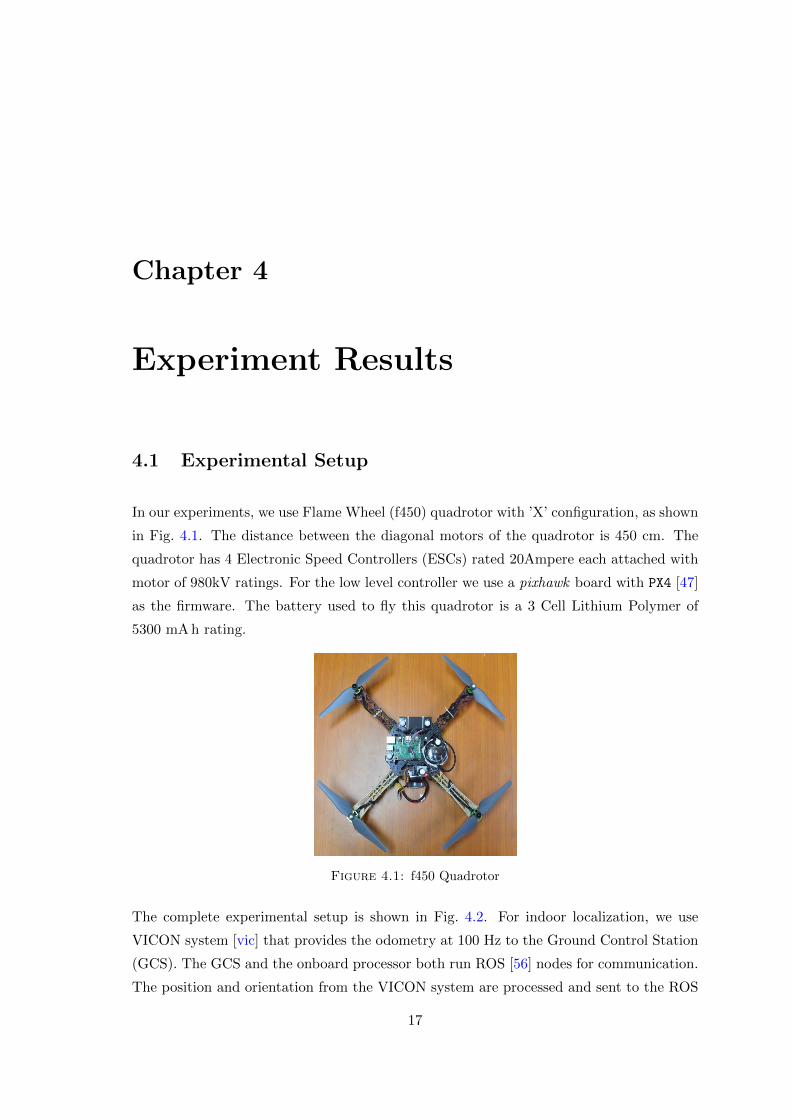
In our experiments, we use Flame Wheel (f450) quadrotor with ’X’ configuration, as shown
in Fig. 4.1. The distance between the diagonal motors of the quadrotor is 450 cm. The
quadrotor has 4 Electronic Speed Controllers (ESCs) rated 20Ampere each attached with
motor of 980kV ratings. For the low level controller we use a pixhawk board with PX4 [47]
as the firmware. The battery used to fly this quadrotor is a 3 Cell Lithium Polymer of
5300 mA h rating.
Figure 4.1: f450 Quadrotor
The complete experimental setup is shown in Fig. 4.2. For indoor localization, we use
VICON system [vic] that provides the odometry at 100 Hz to the Ground Control Station
(GCS). The GCS and the onboard processor both run ROS [56] nodes for communication.
The position and orientation from the VICON system are processed and sent to the ROS
17

Chapter 4. results 18
Figure 4.2: Block diagram of the experimental setup for DeepControl. The GroundStation sends the reference trajectory to the high-level DNN Controller running on-boardin the quadrotor. The low-level attitude controller maintains the desired orientation. The
VICON system provides localization feedback for the controller.
node running on the on-board processor by the GCS. The GCS also publishes the target
position to the on-board processor. The high-level controller running on the on-board
processor takes as input: full state along with the target position from GCS. The output
〈φcmd, θcmd, ψcmd, τcmd〉 is sent to the PX4 running on the pixhawk board. The low-level
PID controller on the pixhawk generates the rotor speed commands that maintain the
desired attitude.
We implement the MPC controller on the flame-wheel using an on-board Odroid XU4 [odr].
The Odroid has an A7 cortex Octa-core processor with 2GB of RAM. The Odroid has a
wifi module that communicates with the GCS. The communication between Odroid and
PX4 on the quadrotor is done using mavlink [Mav] protocol. Similarly, for DNN, we use
the RaspberryPi 3 [ras] as the on-board processor.
4.2 System Identification and Simulation Modelling
For system identification, we manually flew the quadrotor in our lab arena and recorded
the state of quadrotor (st) and control input from the RC transmitter (ut) at time t, using
ROS. We recorded the data at 100Hz. From the recorded data, we calculate the time
constants and the gains. For our quadrotor, the values were : mass: 1.45kg, roll time
constant: 0.185622, pitch time constant: 0.163042, roll gain: 1.037192, and pitch gain:
0.966195.

Chapter 4. results 19
The above constants can define the low-level dynamics of a real-world quadrotor. We
create a simulation model of the f450 quadrotor in Gazebo [41]. The structure of the f450
was obtained from Open-UAV [67]. We tune the gains of low-level PID controllers of the
simulated model such that the transfer function of the simulated model is close to our real-
world f450 quadrotor. The tuning of the PID gains can be done in a few iterations. In our
case, the co-efficient were, for roll: kP = 160, kD = 30, for pitch: kP = 181, kD = 30. We
observe that for the above numbers, the transfer function of the simulated f450 quadrotor
and real-world f450 quadrotor are nearly equal as shown in Fig. 4.3 and Fig. 4.4. The
curve fitting between the commanded attitude and current attitude was 71% for both the
real-world quadrotor and the simulated quadrotor.
Figure 4.3: Orientation tracking of the Real Flame-Wheel 450 quadrotor. The blue linerepresents the orientation of the quadrotor and red line represents the commanded angles.
4.3 Approximating MPC using DNN
The supervised learning requires labeled data. We approximate the MPC by running it on
the simulated quadrotor model. This has several benefits as it saves the time required to
collect the training data by flying the real quadrotor. The flight time of the quadrotor with
fully charged 3-cell battery was observed to be around 15 min with Odroid running on it,
which is quite low for data collection. Instead of charging/recharging batteries multiple
times, we collect the required training data from the simulator model.
We uniformly sample the initial and reference positions for the trajectories of the quadrotor
from an area of size equal to our flying arena: 4m×2m×1m, as shown in Fig. 4.5. We refer

Chapter 4. results 20
Figure 4.4: Orientation tracking of the simulator model of Flame-Wheel 450 quadrotor.The blue line represents the orientation of the quadrotor and red line represents the
commanded angles.
to the difference between the state and the reference at time t as a data-point. We sampled
the data-point and controls at 50Hz over the trajectory in simulation and collected around
1,00,000 data points for the training.
Figure 4.5: Flying Arena
The collected data from the simulator was used to learn the approximate MPC using DNN.
The neural network consists of two fully connected hidden layers with 64 neurons in each
layer. As the yaw is decoupled from the roll, pitch and thrust motion of the quadrotor, we
train our network to predict the three controls: roll, pitch, and thrust. We used Rectified
Linear Unit (ReLU) as the activation function in the hidden states. For the output layer,

Chapter 4. results 21
we use tanh as the activation function.
ReLU(x) = max(0, x)
tanh =ex − e−x
ex + e−x
We minimize the Huber loss between the predicted value and the ground truth value by
using Adam Optimizer [40].
4.4 Comparison of MPC and DNN controllers
For a quantitative comparison of MPC and DNN controller, we fly the quadrotor in dif-
ferent trajectories that can generalize the motions of the quadrotor. We select three types
of trajectories for the evaluation.
• Square: The square trajectory has both roll and pitch movements that are indepen-
dent of each other. This helps in evaluating the roll and pitch outputs of the DNN
and MPC independently. We define the trajectory as a square of size 1m× 1m.
• ∞ Shape: This trajectory has both the roll and pitch motions simultaneously. This
trajectory evaluates the effect of roll and pitch controls when both are dependent on
each other.
• Step Input: This trajectory evaluates the response time of the controller when step
inputs are provided. We provide the setpoint at 30cm apart. We create another
instance of aggressive step input trajectories where setpoints are 1m apart.
All the above three trajectories were generated by using Polynomial trajectory genera-
tor [60], which generates a feasible trajectory for a set of given reference points.
4.4.1 Trajectory Tracking
The trajectory tracking performance of the DNN controller is close to that of the MPC.
The tracking performance of the DNN for independent roll and pitch movements over
the square trajectory is shown in Fig. 4.6. The DNN controller is also able to deal with
the coupled dynamics of the roll and pitch as evident by the tracking of the ∞ shaped

Chapter 4. results 22
Figure 4.6: Comparison of performance between MPC and DNN controllers for trajec-tory of 1m× 1m square for real-world f450 quadrotor.
Figure 4.7: Comparison of performance between MPC and DNN controllers for ∞-shaped trajectory for real-world f450 quadrotor.
Figure 4.8: Comparison of performance between MPC and DNN controller for stepresponse for real-world f450 quadrotor.
trajectory shown in Fig. 4.7. The DNN controller is able to respond to the aggressive step
inputs and shows performance similar to the MPC as shown in Fig. 4.8. The video of the
trajectory tracking is available at https://youtu.be/kWvylnCUUAQ.

Chapter 4. results 23
4.4.2 State cost
We evaluate both the controllers based on the position error with respect to the reference
position. We define the state cost as:
Jpos =T∑t=0
||pt − preft ||2,
where pt is the position at time t, preft the position reference, and ||x||2 denotes the L2-
norm of vector x. We consider the position error to capture the state cost as we have the
reference trajectory in terms of the positions only. The overall performance of the DNN
controller is comparable with the performance of MPC as shown in Table 4.1, in-spite
of the fact that the controller is learned from simulated data and tested on a real-world
quadrotor. The position cost in Table 4.1 is calculated over a flight time of 1min. The
position error for the ∞ shaped trajectory by both the controller is shown in Fig. 4.9.
Figure 4.9: Trajectory tracking error for MPC and DNN controller for ∞ shaped tra-jectory
4.4.3 Control Cost
The control cost has a direct effect on the efficiency of the motor. High control cost
indicates that the motors are stressed by the controller as it generates abrupt changes in
the input. We define control cost for a trajectory as:
Jctrl =
T∑t=0
||ut||2

Chapter 4. results 24
where ut is the control generated at time t.
The control cost of the DNN controller is lower than the MPC as observed from Table 4.1.
This is because of the smoother control signals generated by DNN for ∞ shape trajectory
and step inputs as shown in Fig. 4.10. The DNN gives a smooth output as compared
to MPC due to the fact that during supervised learning, the DNN tires to minimize the
squared error (Huber loss is used in training). This results in a smooth curve fitting by
DNN over the control signals generated by MPC.
Figure 4.10: Comparison of Control signals generated by MPC and DNN for∞ shapedtrajectory and aggressive trajectory (step input).
Trajectory MPC DNNState Cost Control Cost State Cost Control Cost
Square 6.60 0.29 7.56 0.24
∞ shape 16.79 0.71 18.22 0.62
Step Input 28.26 5.43 31.90 4.59
Table 4.1: Comparison of Trajectory cost between MPC and DNN Controller for real-world f450.
4.4.4 Flight Time
We define the flight time of the quadrotor with fully charged 3 cell LiPo battery which has
maximum voltage 12.6 V and capacity 5300 mA h as the total time from initial hover state
to the cutoff voltage defined by PX4: 9.9 V. We observe that the flight time of the quadrotor
has increased for the DNN controller as shown in Table 4.2. The reason is that when we
use the DNN controller, the generated control signals are smooth and the optimization
problem that is solved by the MPC online is replaced with simple matrix operations. The

Chapter 4. results 25
gain in the flight time is more for aggressive trajectories due to the smoother controls
generated by the DNN.
Trajectory Flight Time[secs] % GainMPC DNN
Hover 960 1044 8.75 %
Step Input 922 1020 10.6 %
Aggressive Step Input 902 1015 12.5 %
Table 4.2: Comparison of Flight time between MPC and DNN Controller for real-worldf450
4.4.5 Computational Requirement
We compare the computation cost of the MPC and DNN controller on a single-core ARM
Cortex A7 processor. The MPC solves an online optimization problem by using Acado
solver [34] to generate control signals. The DNN controller performs matrix arithmetic
to calculate the control. The comparison of the computation time is shown in Table 4.3
with both the controllers implemented in C++. For DNN, we use the Eigen library [26]
to perform the matrix arithmetic.
It is also worth noting that the processor hardware required to run the DNN controller
(Raspberrypi 3) is nearly 20% of the cost of the processor hardware required for MPC
(Odroid). The Raspberrypi 3 used for the DNN controller has an ARMv7 processor with
4 cores.
Trajectory MPC DNN
Hover 25 % 3 %
∞ shaped 29 % 4%
Step Input 33 % 4%
Table 4.3: Comparison of CPU usage on a single core ARM Cortex A7 processor.
4.5 Generalization of DNN controller
We evaluate the generalization of the DNN controllers by (i) Evaluating the performance of
DNN on the same quadrotor model with different dynamics (ii) Evaluating the performance
of DNN on a different model, hexarotor :- UAV with 6 rotors.

Chapter 4. results 26
4.5.1 Evaluation on f450
We evaluate the performance of the DNN controller on the f450 model with different
dynamics. We change the mass of the quadrotor and observe that the DNN controller
trained initially is able to track the trajectory for a quadrotor with a different mass.
4.5.1.1 Generating Controller independent of Mass
The DNN controller outputs roll, pitch, yaw rate and thrust. As explained in Section 4.3
, the output layer of the DNN has tanh activation function that maps the output between
-1 and 1. While generating the training data for the controller, the roll, pitch and yaw rate
are converted from degrees to radians. Thereby the range of the attitude controls from
the activation function −1 rad ≤ θ ≤ 1 rad , converted to degrees is −57.29 ≤ θ ≤ 57.29,
which is quite high and encompasses the range of the controls, generated from training
data :−19.48 ≤ θ ≤ 19.48
The thrust is not in the range of tanh, therefore it needs to be adjusted according to the
mass of the quadrotor. We create a mapping between the thrust and mass of the quadrotor
to convert the thrust value in the range of activation function tanh. We generate the
training data for the quadrotor with a mass m0. In the training data, we observe the
mean of the recorded thrust values as τµ. We use a thrust constant, (τµ,m0) to map the
actual thrust (τ) to a range between [−1, 1]: τ[−1,1]. We create a mapping in such a
manner that (i) The mid-value of the range of tanh activation function: [−1, 1] should
map to the mean value of thrust. (ii) The minimum value of the thrust is 0, should map
to the minimum value in the range i.e −1. (iii) The maximum allowed thrust must be
greater than the mean value of the thrust.
We map the τ −→ τ[−1,1] to train the DNN controller, using the equation:
τ[−1,1] =τ − τµ,m0
τµ,m0
(4.1)
While applying the controls after training the DNN controller, we need to remap the values
from τ[−1,1] −→ τ . We calculate the actual values of the thrust by rearranging the Eq. 4.1
as:
τ = τ[−1,1] ∗ τµ,m0 + τµ,m0 (4.2)

Chapter 4. results 27
The value of the mean thrust (τµ) in the training data, depends on the mass of the
quadrotor (m0). When we update the mass of the quadrotor to m, the value of τµ,m0 is
updated using the equation:
τµ,m0 = m ∗ τµ,m0
m0(4.3)
In the experimental setup, we initially generate the training data with a quadrotor mass
of 1.45kilogram. We increase/decrease the weight by 250 gm and evaluate the trajectory
tracking error while using the same initial DNN controller trained for 1.45 Kg. The
parameters for the MPC are updated to the actual mass of the quadrotor.
While generating the training data for the quadrotor of mass 1.45kg, we observe that the
mean value of thrust τµ = 15.51 N. The thrust (τ) is mapped to τ[−1,1] using the Eq. 4.1.
While applying the DNN controller, the values are remapped from τ[−1,1] −→ τ using the
Eq. 4.2. As the mass of the quadrotor is increased/decreased , the value of the constant
τµ,m0 is updated using using Eq. 4.3.
We evaluate the results for a square-shaped trajectory. We record the actual position and
the reference position of the trajectory, at 50 Hz interval. We evaluate the State cost
and Control cost and divide it by the number of points in the trajectory, for both the
controllers. This gives us an idea about the cost of the trajectory per unit point.
Weight [Kg] MPC DNNState Cost Control Cost State Cost Control Cost
1.20 0.092340 0.499790 0.108169 0.497536
1.45 0.091074 0.719129 0.107424 0.716276
1.70 0.095350 0.979669 0.105285 0.976736
1.95 0.093164 1.279866 0.109135 1.276638
Table 4.4: Comparison of Trajectory cost between MPC and DNN Controller for f450with different mass. The DNN controller is trained with the mass of 1.45 Kg.
The results indicate that, on changing the weight of the quadrotor, the DNN controller
can perform the trajectory tracking with efficiency close to the MPC controller. However,
it is important to note that there is a saturation limit of the thrust generated by the
quadrotor, which is restricted by the dimensions of the rotor blades. The dimensions of
the rotor blades determine the total force that the quadrotor can generate. If the mass of
the quadrotor exceeds the sum of forces generated by the rotors, the quadrotor will not
take-off, independent of the controls generated by the controller.

Chapter 4. results 28
Figure 4.11: Comparison of performance between MPC and DNN controller for f450quadrotor.
4.5.2 Evaluation on Firefly
We evaluate the generalization of the DNN controller by implementing the setup for a
hexarotor - AscTec Firefly [asc] for the performance evaluation. The high level trained
DNN controller is able to stabilize and preform the trajectory tracking even for the hexaro-
tor. The results indicate that the DNN controller can be generalized for the number of
rotors in a UAV.
Figure 4.12: Comparison of performance between MPC and DNN controller for infinityshaped trajectory for firefly hexarotor.

Chapter 5
Conclusion
5.1 Contribution
In this thesis, we demonstrate the feasibility of using a Deep Neural Network to approxi-
mate a Model Predictive Controller for a nonlinear dynamical system like quadrotor. We
observe that by modeling the low-level dynamics of the quadrotor in simulation, we are
able to learn the DNN controller for a real-world quadrotor. Through a series of ex-
periments, we evaluate the efficacy of the DNN feedback controller. Our experimental
results demonstrate that the trajectory tracking performance of the DNN based feedback
controller is close to that of the MPC controller. However, the control cost of the DNN
controller is consistently better than the control cost of the MPC controller as the DNN
represents a smooth function. We also measure the flight time for the quadrotor under
both the MPC controller and the DNN controller. Though our test vehicle is quite heavy
and the power consumption to run the motors is significantly more than the power required
for computation, our DNN controller helped in increasing the flight time up to 12.5% for
various reference trajectories. Finally, one major advantage of the DNN controller is that
its hardware requirement is low. The cost of the hardware required to run the DNN con-
troller is only 20% of that of the cost of the hardware required to run the MPC. This helps
us reduce the overall cost of a quadrotor. The results indicate that the Neural Networks
have the potential to become an alternative to classical controllers
29
Chapter 5. Future Work 30
5.2 Future Work
5.2.1 Evaluating the trade-off between the number of layers and perfor-
mance
The number of layers in a deep neural network generally indicates the complexity of the
polynomial learned. We propose to evaluate the effect of the number of layers on the
performance of the DNN controller.
An increase in the layers of the DNN controller should increase the accuracy of the con-
troller. The down-side of increasing the layer is the increase in the computation time for
the controller. In our future work, we plan to experimentally find the optimal number of
layers that provide the maximal performance with predefined computational time bounds.
5.2.2 Reinforcement Learning
The learned controller has its performance limited to the performance of the Model Pre-
dictive Controller. There are factors that can limit the performance of the MPC, for
example, the accuracy of the linearization of the non-linear model and the efficiency of the
optimizer.
We propose to use a Reinforcement Learning based setup to improve the learned controller
through the supervised learning method. The large state-space of the quadrotor makes
policy gradients based algorithms difficult to converge. We propose to use the already
learned controller as a Guide to the Actor-Critic setup of the policy gradient-based algo-
rithms. The guide network has already some information about the control space of the
quadrotor (learned from MPC). The policy search space can be decreased by augmenting
the actor-network with the guide network.
5.2.3 Robustness of the Neural Network based controller
We propose to perform the robustness analysis of the closed-loop of non-linear plant and
neural-network-based controller by evaluating the set of states reached by the plant with
the DNN controller. This requires the computation of the bounds on the state of the
plant for a given range of control inputs. We can calculate the bounds on the set of states
reached by the plant using tools like SpaceEx [22]. Similarly, we can calculate the bound
on the output of the DNN controller using existing tools like ERAN [73].

Chapter 5. Future Work 31
This bound propagation and from controller output to plant states can ensure that the
plant does not reach an unsafe state if it starts from a particular set of the initial state.

Bibliography
[asc] Asctec firefly. Website. [Online] http://www.asctec.de/en/
uav-uas-drones-rpas-roav/asctec-firefly/.
[cf2] Crazyflie 2.0.
[Mav] MAVlink (2014) MAVlink micro air vehicle protocol. Website. [Online] http://
mavlink.org.
[odr] ODROID XU4. Website. [Online] https://www.hardkernel.com.
[ras] Raspberrypi 3. Website. [Online] https://www.raspberrypi.org/products/
raspberry-pi-3-model-b/.
[vic] VICON motion capture system. Website. [Online] http://www.vicon.com/.
[7] Abbeel, P., Coates, A., and Ng, A. Y. (2010). Autonomous helicopter aerobatics
through apprenticeship learning. I. J. Robotics Res., 29(13):1608–1639.
[8] Allgower, F., Findeisen, R., and Nagy, Z. K. (2004). Nonlinear model predictive control:
From theory to application. J. Chin. Inst. Chem. Engrs., 35(3):299–315.
[9] Astrom, K. J. and Murray, R. M. (2010). Feedback systems: an introduction for sci-
entists and engineers. Princeton university press.
[10] Ba, L. J., Kiros, R., and Hinton, G. E. (2016). Layer normalization. CoRR,
abs/1607.06450.
[11] Bansal, S., Akametalu, A. K., Jiang, F. J., Laine, F., and Tomlin, C. J. (2016).
Learning quadrotor dynamics using neural network for flight control. In CDC, pages
4653–4660.
[12] Beard, R. (2008). Quadrotor dynamics and control rev 0.1.
32

Bibliography 33
[13] Bemporad, A., Manfred, M., Dua, V., and Pistikopoulos, E. N. (2002). The explicit
linear quadratic regulator for constrained systems. Automatica, 38(1):3–20.
[14] Berkenkamp, F., Turchetta, M., Schoellig, A. P., and Krause, A. (2017). Safe model-
based reinforcement learning with stability guarantees. In NIPS, pages 908–918.
[15] Bottou, L. (2010). Large-scale machine learning with stochastic gradient descent. In
Proceedings of COMPSTAT’2010, pages 177–186. Springer.
[16] Bouffard, P. (2012). On-board model predictive control of a quadrotor helicopter:
Design, implementation, and experiments. Technical report, University of California
Berkeley.
[17] Bresciani, T. (2008). Modelling, identification and control of a quadrotor helicopter.
MSc Theses.
[18] Brockman, G., Cheung, V., Pettersson, L., Schneider, J., Schulman, J., Tang, J., and
Zaremba, W. (2016). Openai gym.
[19] Chen, S., Saulnier, K., Atanasov, N., Lee, D. D., Kumar, V., Pappas, G. J., and
Morari, M. (2018). Approximating explicit model predictive control using constrained
neural networks. In ACC, pages 1520–1527.
[20] Chow, Y., Nachum, O., Duenez-Guzman, E. A., and Ghavamzadeh, M. (2018). A
lyapunov-based approach to safe reinforcement learning. In NeurIPS, pages 8103–8112.
[21] Diebel, J. (2006). Representing attitude: Euler angles, unit quaternions, and rotation
vectors. Matrix, 58(15-16):1–35.
[22] Frehse, G., Le Guernic, C., Donze, A., Cotton, S., Ray, R., Lebeltel, O., Ripado, R.,
Girard, A., Dang, T., and Maler, O. (2011). Spaceex: Scalable verification of hybrid
systems. In Ganesh Gopalakrishnan, S. Q., editor, Proc. 23rd International Conference
on Computer Aided Verification (CAV), LNCS. Springer.
[23] Furrer, F., Burri, M., Achtelik, M., and Siegwart, R. (2016). Robot Operating System
(ROS): The Complete Reference (Volume 1), chapter RotorS – A Modular Gazebo MAV
Simulator Framework, pages 595–625. Springer International Publishing, Cham.
[24] Garcia, C. E., Prett, D. M., and Morari, M. (1989). Model predictive control: Theory
and practice - a survey. Automatica, 25(3):335 – 348.
[25] Goodfellow, I., Bengio, Y., and Courville, A. (2016). Deep learning. MIT press.

Bibliography 34
[26] Guennebaud, G., Jacob, B., et al. (2010). Eigen v3. http://eigen.tuxfamily.org.
[27] Hagan, M. T., Demuth, H. B., Beale, M. H., and Jesus, O. D. (1996). Neural network
design, volume 20. Pws Pub. Boston.
[28] Han, J. and Moraga, C. (1995). The influence of the sigmoid function parameters on
the speed of backpropagation learning. In International Workshop on Artificial Neural
Networks, pages 195–201. Springer.
[29] Haykin, S. (1994). Neural networks, volume 2. Prentice Hall New York.
[30] Hecht-Nielsen, R. (1992). Theory of the backpropagation neural network. In Neural
networks for perception, pages 65–93. Elsevier.
[31] Henderson, P., Islam, R., Bachman, P., Pineau, J., Precup, D., and Meger, D. (2018).
Deep reinforcement learning that matters. In Thirty-Second AAAI Conference on Ar-
tificial Intelligence.
[32] Hinton, G., Deng, L., Yu, D., Dahl, G., Mohamed, A. R., Jaitly, N., Senior, A.,
Vanhoucke, V., Nguyen, P., Kingsbury, B., et al. (2012). Deep neural networks for
acoustic modeling in speech recognition. IEEE Signal processing magazine, 29.
[33] Hoffmann, G., Huang, H., Waslander, S., and Tomlin, C. (2007). Quadrotor helicopter
flight dynamics and control: Theory and experiment. In AIAA guidance, navigation and
control conference and exhibit, page 6461.
[34] Houska, B., Ferreau, H. J., and Diehl, M. (2010). ACADO toolkit – An open-source
framework for automatic control and dynamic optimization. Optimal Control Applica-
tions and Methods, 32(3):298–312.
[35] Huber, P. J. et al. (1964). Robust estimation of a location parameter. The annals of
mathematical statistics, 35(1):73–101.
[36] Hwangbo, J., Sa, I., Siegwart, R., and Hutter, M. (2017). Control of a quadrotor with
reinforcement learning. IEEE Robotics and Automation Letters, 2(4):2096–2103.
[37] Kaelbling, L. P., Littman, M. L., and Moore, A. W. (1996). Reinforcement learning:
A survey. Journal of Artificial Intelligence Research, page 237–285.
[38] Kalman, R. E. et al. (1960). Contributions to the theory of optimal control. Bol. soc.
mat. mexicana, 5(2):102–119.
Bibliography 35
[Kamel et al.] Kamel, M., Stastny, T., Alexis, K., and Siegwart, R. Model predictive
control for trajectory tracking of unmanned aerial vehicles using robot operating system.
In Koubaa, A., editor, Robot Operating System (ROS) The Complete Reference, Volume
2. Springer.
[40] Kingma, D. P. and Ba, J. (2014). Adam: A method for stochastic optimization. arXiv
preprint arXiv:1412.6980.
[41] Koenig, N. and Howard, A. (2004). Design and use paradigms for Gazebo, an open-
source multi-robot simulator. In IROS, pages 2149–2154.
[42] Landry, B. et al. (2015). Planning and control for quadrotor flight through cluttered
environments. PhD thesis, Massachusetts Institute of Technology.
[43] Li, Q., Qian, J., Zhu, Z., Bao, X., Helwa, M. K., and Schoellig, A. P. (2017). Deep
neural networks for improved, impromptu trajectory tracking of quadrotors. In ICRA,
pages 5183–5189.
[44] Lillicrap, T. P., Hunt, J. J., Pritzel, A., Heess, N., Erez, T., Tassa, Y., Silver, D.,
and Wierstra, D. (2015a). Continuous control with deep reinforcement learning. CoRR,
abs/1509.02971.
[45] Lillicrap, T. P., Hunt, J. J., Pritzel, A., Heess, N., Erez, T., Tassa, Y., Silver, D.,
and Wierstra, D. (2015b). Continuous control with deep reinforcement learning. arXiv
preprint arXiv:1509.02971.
[46] Martin, P. and Salaun, E. (2010). The true role of accelerometer feedback in quadrotor
control. In 2010 IEEE International Conference on Robotics and Automation, pages
1623–1629. IEEE.
[47] Meier, L., Honegger, D., and Pollefeys, M. (2015). PX4: A node-based multithreaded
open source robotics framework for deeply embedded platforms. ICRA, pages 6235–
6240.
[48] Mellinger, D. and Kumar, V. (2011a). Minimum snap trajectory generation and
control for quadrotors. In ICRA, pages 2520–2525.
[49] Mellinger, D. and Kumar, V. (2011b). Minimum snap trajectory generation and
control for quadrotors. In ICRA, pages 2520–2525. IEEE.
[50] Nair, A., McGrew, B., Andrychowicz, M., Zaremba, W., and Abbeel, P. (2017).
Overcoming exploration in reinforcement learning with demonstrations. CoRR,
abs/1709.10089.

Bibliography 36
[51] Nair, V. and Hinton, G. E. (2010). Rectified linear units improve restricted Boltzmann
machines. In ICML, pages 807–814.
[52] Nicol, C., Macnab, C. B., and Ramirez-Serrano, A. (2011). Robust adaptive control
of a quadrotor helicopter. Mechatronics, 21(6):927–938.
[53] Nicol, C., Macnab, C. J. B., and Ramirez-Serrano, A. (2008). Robust neural net-
work control of a quadrotor helicopter. In 2008 Canadian Conference on Electrical and
Computer Engineering, pages 001233–001238.
[54] Pan, S. J. and Yang, Q. (2010). A survey on transfer learning. IEEE Transactions
on Knowledge and Data Engineering, 22:1345–1359.
[55] Quigley, M., Conley, K., Gerkey, B., Faust, J., Foote, T., Leibs, J., Wheeler, R., and
Ng, A. Y. (2009a). Ros: an open-source robot operating system. In ICRA workshop on
open source software, volume 3, page 5. Kobe, Japan.
[56] Quigley, M., Gerkey, B., Conley, K., Faust, J., Foote, T., Leibs, J., Berger, E.,
Wheeler, R., and Ng, A. (2009b). ROS: an open-source robot operating system. In
ICRA Workshop on Open Source Robotics.
[57] Raffo, G. V., Ortega, M. G., and Rubio, F. R. (2010). An integral predictive/nonlinear
H-∞ control structure for a quadrotor helicopter. Automatica, 46(1):29–39.
[58] Rawlings, J. B. and Mayne, D. (2009). Model predictive control: Theory and design.
Nob Hill Pub. Madison, Wisconsin.
[59] Richards, S. M., Berkenkamp, F., and Krause, A. (2018). The lyapunov neural
network: Adaptive stability certification for safe learning of dynamic systems. arXiv
preprint arXiv:1808.00924.
[60] Richter, C., Bry, A., and Roy, N. (2016). Polynomial trajectory planning for aggressive
quadrotor flight in dense indoor environments. In Robotics Research, pages 649–666.
Springer.
[61] Rivera, D. E., Morari, M., and Skogestad, S. (1986). Internal model control: PID
controller design. Industrial & engineering chemistry process design and development,
25(1):252–265.
[62] Russell, S. J. and Norvig, P. (2010). Artificial Intelligence: A Modern Approach.
Prentice Hall, third edition.

Bibliography 37
[63] Sabatino, F. (2015). Quadrotor control: modeling, nonlinearcontrol design, and sim-
ulation.
[64] Salih, A. L., Moghavvemi, M., Mohamed, H. A. F., and Gaeid, K. S. (2010). Flight
PID controller design for a uav quadrotor. Scientific research and essays, 5(23):3660–
3667.
[65] Sanchez, C. S. and Izzo, D. (2018). Real-time optimal control via deep neural net-
works: study on landing problems. Journal of Guidance, Control, and Dynamics,
41(5):1122–1135.
[66] Schaul, T., Quan, J., Antonoglou, I., and Silver, D. (2015). Prioritized experience
replay. arXiv preprint arXiv:1511.05952.
[67] Schmittle, M., Lukina, A., Vacek, L., Das, J., Buskirk, C. P. V., Rees, S., Sztipanovits,
J., Grosu, R., and Kumar, V. (2018). OpenUAV: A UAV testbed for the CPS and
robotics community. ICCPS, pages 130–139.
[68] Schulman, J., Ho, J., Lee, A. X., Awwal, I., Bradlow, H., and Abbeel, P. (2013).
Finding locally optimal, collision-free trajectories with sequential convex optimization.
In Robotics: science and systems, volume 9, pages 1–10.
[69] Schulman, J., Levine, S., Moritz, P., Jordan, M. I., and Abbeel, P. (2015). Trust
region policy optimization. CoRR, abs/1502.05477.
[70] Schulman, J., Wolski, F., Dhariwal, P., Radford, A., and Klimov, O. (2017). Proximal
policy optimization algorithms. CoRR, abs/1707.06347.
[71] Silver, D., Lever, G., Heess, N., Degris, T., Wierstra, D., and Riedmiller, M. (2014).
Deterministic policy gradient algorithms. In ICML.
[72] Simonyan, K. and Zisserman, A. (2014). Very deep convolutional networks for large-
scale image recognition. arXiv preprint arXiv:1409.1556.
[73] Singh, G., Gehr, T., Mirman, M., Puschel, M., and Vechev, M. (2018). Fast and
effective robustness certification. In Advances in Neural Information Processing Systems,
pages 10802–10813.
[74] Sutton, R. S. and Barto, A. G. (1998). Reinforcement Learning: An Introduction.
The MIT Press.

Bibliography 38
[75] Sutton, R. S., McAllester, D. A., Singh, S. P., and Mansour, Y. (2000). Policy gradient
methods for reinforcement learning with function approximation. In Advances in neural
information processing systems, pages 1057–1063.
[76] Taylor, M. E. and Stone, P. (2009). Transfer learning for reinforcement learning
domains: A survey. Journal of Machine Learning Research, page 1633–1685.
[77] Tondel, P., Johansen, T. A., and Bemporad, A. (2001). An algorithm for multi-
parametric quadratic programming and explicit MPC solutions. In CDC, pages 1199–
1204.
[78] Visioli, A. (2006). Practical PID Control. Advances in Industrial Control. Springer
London.
[79] Voos, I. (2009). Nonlinear control of a quadrotor micro-uav using feedback-
linearization. In IEEE International Conference on Mechatronics, pages 1–6.
[80] Xu, R. and Ozguner, U. (2006). Sliding mode control of a quadrotor helicopter. In
CDC, pages 4957–4962.
[81] Zhang, T., Kahn, G., Levine, S., and Abbeel, P. (2016). Learning deep control policies
for autonomous aerial vehicles with MPC-guided policy search. In ICRA, pages 528–535.