control of salinity on the mixed layer depth in the world ocean: 1...

Control of salinity on the mixed layer depth in the

world ocean:

1. General description

Clement de Boyer Montegut,1 Juliette Mignot,2 Alban Lazar,2 and Sophie Cravatte3

Received 6 October 2006; revised 11 January 2007; accepted 26 January 2007; published 19 June 2007.

[1] Using instantaneous temperature and salinity profiles, including recent Argo data, aglobal ocean climatology of monthly mean properties of the ‘‘barrier layer’’ (BL)phenomenon is constructed. This climatology is based on the individual analysis ofinstantaneous profiles in contrast with previous large-scale climatologies derived fromgridded fields. This ensures a more accurate description of the BL phenomenon. Wedistinguish three types of regions: BLs are quasi-permanent in the equatorial andwestern tropical Atlantic and Pacific, the Bay of Bengal, the eastern equatorial IndianOcean, the Labrador Sea, and parts of the Arctic and Southern Ocean. In the northernsubpolar basins, the southern Indian Ocean, and the Arabian Sea, BLs are ratherseasonal. Finally, BLs are typically never detected between 25� and 45� latitude in eachbasin. Away from the deep tropics, the analysis reveals strong similarities between thetwo hemispheres and the three oceans regarding BL seasonality and formationmechanisms. Temperature inversions below the mixed layer are often associated withBLs. Their typical amplitude, depth, and seasonality are described here for the first timeat global scale. We suggest that this global product could be used as a reference forfuture studies and to validate the representation of upper oceanic layers by generalcirculation models.

Citation: de Boyer Montegut, C., J. Mignot, A. Lazar, and S. Cravatte (2007), Control of salinity on the mixed layer depth in the

world ocean: 1. General description, J. Geophys. Res., 112, C06011, doi:10.1029/2006JC003953.

1. Introduction

[2] Classically, the vertical structure of the upper oceancan be schematically divided into two layers: a near surfacelayer where temperature and salinity are well mixed and thedeeper stratified ocean. The near-surface mixed layer is thesite of active air-sea interaction. The transfer of mass,momentum, and energy between the atmosphere and thishomogeneous layer is the source of most oceanic motionsand at short timescales (a day or a few days), its thicknessdetermines the thermal and mechanical inertia of the upperocean. In a stable ocean, water density is minimum in thislayer. It is separated from the ocean interior by a strongvertical density gradient, also called pycnocline.[3] Definitions of the mixed layer depth are most com-

monly based on a stratification criteria: the base of themixed layer is usually defined as the top of the pycnocline,being the depth where the density has increased by a certain

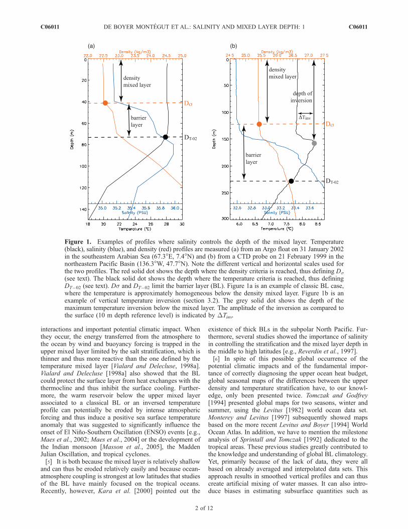
threshold from its surface value. In practice, given the lackof salinity data, scientists have often concentrated on thetemperature stratification, assuming that the top of thethermocline and halocline have the same depth and thustogether define that of the pycnocline. However, this view issimplified and in the real ocean, the situation is frequentlydifferent, as a result of specific thermal and haline forcings.Situations where the top of the halocline is shallower thanthat of the thermocline have been observed since the 1960s[Defant, 1961; Rotschi et al., 1972; Lukas and Lindstrom,1987; Lindstrom et al., 1987] and baptized the ‘‘barrierlayer’’ phenomenon at the end of the 1980s [Godfrey andLindstrom, 1989]. Instead of two, the vertical structure ofthe upper ocean is then divided into three layers (Figure 1):the mixed layer, limited by the top of the halocline (thatdefines the top of the pycnocline in that case), the so-calledbarrier layer (BL), confined between the top of the haloclineand of the thermocline, and the deep ocean. Schematically,the temperature in the BL is constant and equal to that in themixed layer (Figure 1a). In some cases, however, thesalinity stratification is such that the stability of the oceancan even support a temperature increase in subsurface [e.g.,Shankar et al., 2004]. The latter then reaches a subsurfacemaximum within the BL before decreasing again at greaterdepth (Figure 1b).[4] BLs (associated with a subsurface temperature inver-

sion or not) have important consequences on the air-sea

JOURNAL OF GEOPHYSICAL RESEARCH, VOL. 112, C06011, doi:10.1029/2006JC003953, 2007ClickHere

for

FullArticle

1Frontier Research Center for Global Change, Japan Agency forMarine-Earth Science and Technology, Yokohama, Japan.

2Laboratoire d’Oceanographie et du Climat: Experimentations etApproches Numeriques, Institut Pierre Simon Laplace, Unite Mixte deRecherche, CNRS/IRD/UPMC, Paris, France.

3Laboratoire d’Etudes en Geophysique et Oceanographie Spatiales,Unite Mixte de Recherche, CNRS/IRD/CNES/Universite Paul Sabatier,Toulouse, France.

Copyright 2007 by the American Geophysical Union.0148-0227/07/2006JC003953$09.00

C06011 1 of 12

http://dx.doi.org/10.1029/2006JC003953

interactions and important potential climatic impact. Whenthey occur, the energy transferred from the atmosphere tothe ocean by wind and buoyancy forcing is trapped in theupper mixed layer limited by the salt stratification, which isthinner and thus more reactive than the one defined by thetemperature mixed layer [Vialard and Delecluse, 1998a].Vialard and Delecluse [1998a] also showed that the BLcould protect the surface layer from heat exchanges with thethermocline and thus inhibit the surface cooling. Further-more, the warm reservoir below the upper mixed layerassociated to a classical BL or an inversed temperatureprofile can potentially be eroded by intense atmosphericforcing and thus induce a positive sea surface temperatureanomaly that was suggested to significantly influence theonset of El Nino-Southern Oscillation (ENSO) events [e.g.,Maes et al., 2002; Maes et al., 2004] or the development ofthe Indian monsoon [Masson et al., 2005], the MaddenJulian Oscillation, and tropical cyclones.[5] It is both because the mixed layer is relatively shallow

and can thus be eroded relatively easily and because ocean-atmosphere coupling is strongest at low latitudes that studiesof the BL have mainly focused on the tropical oceans.Recently, however, Kara et al. [2000] pointed out the

existence of thick BLs in the subpolar North Pacific. Fur-thermore, several studies showed the importance of salinityin controlling the stratification and the mixed layer depth inthe middle to high latitudes [e.g., Reverdin et al., 1997].[6] In spite of this possible global occurrence of the

potential climatic impacts and of the fundamental impor-tance of correctly diagnosing the upper ocean heat budget,global seasonal maps of the differences between the upperdensity and temperature stratification have, to our knowl-edge, only been presented twice. Tomczak and Godfrey[1994] presented global maps for two seasons, winter andsummer, using the Levitus [1982] world ocean data set.Monterey and Levitus [1997] subsequently showed mapsbased on the more recent Levitus and Boyer [1994] WorldOcean Atlas. In addition, we have to mention the milestoneanalysis of Sprintall and Tomczak [1992] dedicated to thetropical areas. These previous studies greatly contributed tothe knowledge and understanding of global BL climatology.Yet, primarily because of the lack of data, they were allbased on already averaged and interpolated data sets. Thisapproach results in smoothed vertical profiles and can thuscreate artificial mixing of water masses. It can also intro-duce biases in estimating subsurface quantities such as

Figure 1. Examples of profiles where salinity controls the depth of the mixed layer. Temperature(black), salinity (blue), and density (red) profiles are measured (a) from an Argo float on 31 January 2002in the southeastern Arabian Sea (67.3�E, 7.4�N) and (b) from a CTD probe on 21 February 1999 in thenortheastern Pacific Basin (136.3�W, 47.7�N). Note the different vertical and horizontal scales used forthe two profiles. The red solid dot shows the depth where the density criteria is reached, thus defining Ds(see text). The black solid dot shows the depth where the temperature criteria is reached, thus definingDT�02 (see text). Ds and DT�02 limit the barrier layer (BL). Figure 1a is an example of classic BL case,where the temperature is approximately homogeneous below the density mixed layer. Figure 1b is anexample of vertical temperature inversion (section 3.2). The grey solid dot shows the depth of themaximum temperature inversion below the mixed layer. The amplitude of the inversion as compared tothe surface (10 m depth reference level) is indicated by DTinv.

C06011 DE BOYER MONTEGUT ET AL.: SALINITY AND MIXED LAYER DEPTH: 1

2 of 12

C06011

barrier layer thickness (BLT) or mixed layer depth [deBoyer Montegut et al., 2004]. More recently, other authorshave used individual profiles, thereby retaining more de-tailed structures, but their studies only concerned limitedarea [e.g., Ando and McPhaden, 1997; Sato et al., 2004; Quand Meyers, 2005]. Here, we present for the first time aglobal climatology of the differences between the upperdensity and temperature stratification based on the analysisof most of the available instantaneous profiles of the upperocean. Our aim is to give a global insight into the occur-rence, seasonality, and order of magnitude of these differ-ences and thus to better document and understand thecontrol of the mixed layer by salinity in the world ocean.Our objective is also to present a new global product that webelieve is of high interest for model validations andimprovements or studies of the upper ocean budgets. Ourproduct shows that the control of the mixed layer by salinityis a global phenomenon, primarily at play in winter.[7] The data set and methodology is presented in the

following section. Global maps documenting the seasonsand areas where the salinity has a substantial influence onthe vertical stratification of the upper ocean are described insection 3. Temperature inversions below the mixed layer

will also be introduced in that section, and BL criteria willbe discussed in light of these results. Section 4 focuses onthe subpolar and polar regions, where large temperatureinversions are detected, while a companion paper [Mignot etal., 2007] is entirely dedicated to the tropical areas. Con-clusions are given in section 5.

2. Data Set and Method

2.1. Data Set

[8] This study is based on the collection of more than500,000 instantaneous temperature and salinity profilescollected between 1967 and 2002 and obtained from theNational Oceanographic Data Center (NODC) and from theWorld Ocean Circulation Experiment (WOCE) database,complemented by those available between 1996 and January2006 from the Argo Global Data Centers (GDAC). The firsttwo databases were used by de Boyer Montegut et al. [2004]to construct a new global mixed layer depth climatology. Theglobal array of profiling floats, Argo, returning now around100,000 profiles of temperature and salinity per year is thegreatest source of observations for ocean subsurface. Itrepresents approximately 30% of the total amount of profiles

Figure 2. Distribution of profiles in each 2� by 2� mesh box. (a) Profiles with both temperature andsalinity data, used to compute the barrier layer thickness (BLT) climatology (Figure 3). (b) Profiles withtemperature data used to build the temperature inversion maps (Figure 6). Data are taken from theNational Oceanographic Data Center, World Ocean Circulation Experiment, and Argo database between1967 (first year with CTD salinity profiles) and 2006. JFM and JAS indicate the two seasons January-February-March and July-August-September, respectively.


3 of 12

C06011

we use in this study. The seasonal spatial distributions of thedata are shown in Figure 2. Figure 2a can be compared withFigure 1b of de Boyer Montegut et al. [2004] whichrepresents the temperature-salinity profiles distribution with-out Argo database. A striking improvement is the reductionof the sparsity of salinity data in every oceans and especiallyin the Southern Ocean. Even if some areas have a shorttemporal coverage with a likely trend toward the recentyears, such a distribution now allows us to construct areliable monthly climatology of subsurface ocean variables(e.g., mixed layer depth, BLT. . .) based on both temperatureand salinity observations.[9] Additionally, we also used Expendable Bathythermo-

graph (XBT) and Mechanical Bathythermograph (MBT)temperature profiles from NODC when investigating theoccurrence of temperature inversions below the mixed layer(cf. section 3.2). Figure 2b shows the distribution of alltemperature profiles available between 1967 and 2006. Evenif the benefits of adding Argo data is less impressive thanwith salinity data, it still represents a considerable improve-ment in coverage of the southern part of the three oceans.[10] The reader is referred to de Boyer Montegut et al.

[2004] for a detailed description of the data analysis. Theaverage vertical resolution of the profiles are 8.2 m, 2.3 m,19.5 m, 9.4 m, and 10.5 m for profiling floats (PFL),conductivity-temperature-depth (CTD), XBT, MBT, andArgo profilers respectively.

2.2. Methodology

[11] As in the work of de Boyer Montegut et al. [2004], the2� spatial resolution climatology described below is based ondirect estimates of the temperature and density stratificationfrom individual profiles with data at observed levels. This is adifferent and better approach from the one based on averagedprofiles [Tomczak and Godfrey, 1994;Monterey and Levitus,1997] that can be altered by optimal interpolation and mayhave misleading information such as artificial density inver-sions or false vertical gradients, especially in areas of sparsedata [Lozier et al., 1994]. Analyzing individual profilesallows a more detailed and realistic description and thusgives more confidence in the investigation of the physicalprocesses at stake. Unless otherwise indicated, ordinarykriging limited to a 1000-km radius disk containing at least5 grid point values was used to grid the obtained fields.Kriging is an optimal prediction method very often used inspatial data analysis. It has close links to objective analysis. Itis based on statistical principles and on the assumption thatthe parameter being interpolated can be treated as a region-alized variable, which is true for BLT. One advantage of thisgeostatistical approach to interpolation is that kriging is anexact interpolator, which does not change any known values.Given the fact that Argo data now offer a very good coverageof the oceans (more than 50% of the 2 degree grid points arecovered in the tropics every month), we can note thatdifferent values of the radius of kriging (500, 1000, or1500 km) barely changes the final fields. Difference betweenthose ones are less than 5m everywhere except locally at highlatitudes (e.g., in austral ocean during winter).

2.3. BL Criterion

[12] In order to characterize the vertical structure oftemperature in the upper ocean and to diagnose the top of

the oceanic thermocline, we define the depth DT�02 wherethe temperature has decreased by 0.2�C as compared to thetemperature at the reference depth of 10m. Although theremight be regions and seasons where the temperature (anddensity) mixed layer is shallower than 10 m (in areas ofstrong upwelling in particular), this choice is made in orderto have the same reference for all areas and to avoid thediurnal variability of temperature and/or density stratifica-tion in the top few meters of the ocean. The threshold 0.2�Cwas diagnosed by de Boyer Montegut et al. [2004] as themost appropriate for mixed layer depth estimation fromindividual profiles.[13] Following most previous authors who studied the BL

[e.g., Lukas and Lindstrom, 1991; Sprintall and Tomczak,1992; Vialard and Delecluse, 1998a], we define also thedepth Ds where the potential density sq has increased fromthe reference depth by a threshold Ds equivalent to thedensity difference for the same temperature change atconstant salinity:

Ds ¼ sq T10 � 0:2; S10;P0ð Þ � sq T10; S10;P0ð Þ ð1Þ

where T10 and S10 are the temperature and salinity at thereference depth 10 m and P0 is the pressure at the oceansurface. Because of oceanic stability, the density isnecessarily approximately constant above this depth, whichdefines thus the base of the density mixed layer. In theidealized situations defined in the introduction where thetemperature and density are well mixed until the samedepth, then DT�02 = Ds (slight differences can still beexpected in areas where temperature and salinity variationsare coupled). However, this is not necessarily the casebecause of the independence of temperature and salinity andthe possible influence of salinity on the upper oceanstability and stratification. As explained in the introduction,the intermediate layer then constitutes the BL and itsthickness is defined as the difference between DT�02 and Ds(Figure 1). Note that a BL implies constraints both onsalinity and temperature stratifications: the former must bewell-marked at relatively shallow depth, while the lattermust be reached either at a deeper level or must becharacterized by a vertical inversion of the thermal gradient,achieved when the temperature reaches a subsurfacemaximum before the negative threshold (Figure 1).

3. General Description of the Product

3.1. Global Differences Between Temperature andSalinity Stratification in the Upper Ocean

[14] Figures 3, 4, and 5 illustrate three major aspects ofthe global pattern of BLT, defined as DT�02 � Ds for thepurposes of this paper. Namely, Figure 3 shows its seasonalspatial distribution, Figure 4 the thickest BL detected over aseasonal cycle at each grid point and Figure 5 the number ofmonths during which a significant BL is detected. Thesemaps show very clearly that unlike what the past literatureon BLs suggest, they are a global phenomenon, which notonly concerns the tropics but also higher latitudes. Excep-tion of the midlatitudes (25�–45�) must however be under-lined, as detailed below. Apart from these latitudinal bands,BLs are thickest in the winter hemisphere (Figure 3), and


4 of 12

C06011

maximum thickness can then exceed 100 m in the subpolarand polar areas (Figure 4). In the tropical areas, maximumthickness is rather around 40 to 50 m. Note that in theseregions, there is a nice spatial correlation between Figure 4and Figure 5: thickest BLs are the most persistent.[15] In terms of duration (Figure 5), one can distinguish

three types of BL regions: in the equatorial and westerntropical Pacific and Atlantic, the Bay of Bengal and easternequatorial Indian Ocean, the Labrador Sea, and parts of theArctic and the Southern Ocean, BLs are typically signifi-cantly present during at least 10 months per year. They canthus be considered as quasi-permanent. In the Arctic andthe Southern Ocean, the lack of data might artificiallyreduce the extent and length of the BLs detected with theproduct (see hatches in Figure 5). Seasonal BLs, lastingabout 6 months, are detected in the northern subpolarbasins, in the Arabian Sea as well as in the southernIndian Ocean, and equatorward of the subtropical salinitymaxima, as is described in a companion paper [Mignot etal., 2007]. The third type of area consists in regions whereBLs are nearly never detected. They are located around 25to 45� latitude in both hemispheres and all basins, as well

as along the eastern subtropical oceanic boundaries. Upw-ellings taking place in the latter areas maintain a veryshallow mixed layer and ensure a temperature and salinitystratification down to the same depth.[16] The equatorial and tropical BLs are easily identified

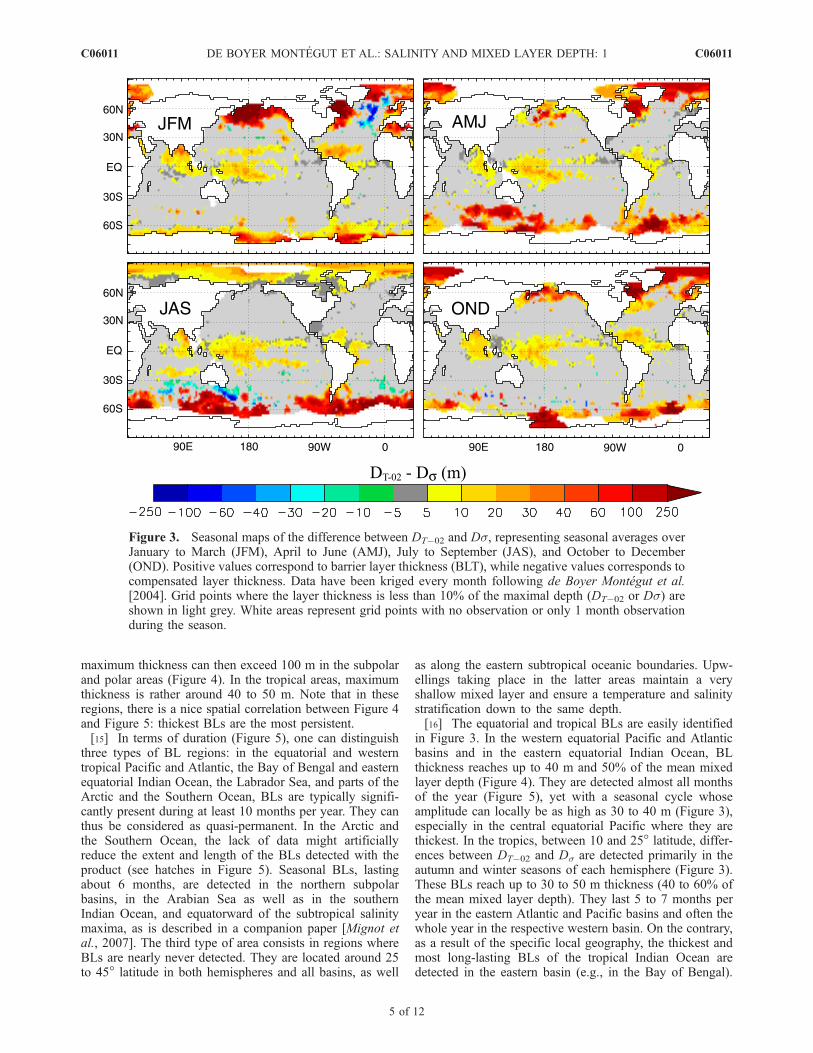
in Figure 3. In the western equatorial Pacific and Atlanticbasins and in the eastern equatorial Indian Ocean, BLthickness reaches up to 40 m and 50% of the mean mixedlayer depth (Figure 4). They are detected almost all monthsof the year (Figure 5), yet with a seasonal cycle whoseamplitude can locally be as high as 30 to 40 m (Figure 3),especially in the central equatorial Pacific where they arethickest. In the tropics, between 10 and 25� latitude, differ-ences between DT�02 and Ds are detected primarily in theautumn and winter seasons of each hemisphere (Figure 3).These BLs reach up to 30 to 50 m thickness (40 to 60% ofthe mean mixed layer depth). They last 5 to 7 months peryear in the eastern Atlantic and Pacific basins and often thewhole year in the respective western basin. On the contrary,as a result of the specific local geography, the thickest andmost long-lasting BLs of the tropical Indian Ocean aredetected in the eastern basin (e.g., in the Bay of Bengal).

Figure 3. Seasonal maps of the difference between DT�02 and Ds, representing seasonal averages overJanuary to March (JFM), April to June (AMJ), July to September (JAS), and October to December(OND). Positive values correspond to barrier layer thickness (BLT), while negative values corresponds tocompensated layer thickness. Data have been kriged every month following de Boyer Montegut et al.[2004]. Grid points where the layer thickness is less than 10% of the maximal depth (DT�02 or Ds) areshown in light grey. White areas represent grid points with no observation or only 1 month observationduring the season.


5 of 12

C06011

A more detailed description of these regions is given byMignot et al. [2007].[17] Poleward,in the subtropical gyres (roughly between

25 and 45� of latitude), the difference DT�02 � Ds is mostoften negative, meaning that Ds is detected at greater depththan DT�02. This implies that the temperature stratificationbelow the well-mixed layer is partially compensated by astratification in salinity so that the density profile is close tovertical homogeneity on a greater depth than the mixedlayer. Overall, BLs can only appear by definition in regionswith fresher water in the surface layer than in the subsurfaceone. Indeed, those compensation regions correspond roughlyto decrease of salinity below the mixed layer (not shown). Incase of substantial compensation, the corresponding type ofmixed layer is described as ‘‘vertically compensated’’ [e.g.,Stommel and Fedorov, 1967; de Boyer Montegut et al.,2004]. Such layers are typically detected in the winter

season of each hemisphere and they are most prominentin the northeastern Atlantic and in the Southern Ocean(Figure 3). They are also present in the midlatitudebasins (Pacific and Atlantic), but they do not reach the10% criterion used in Figure 3 and they are thus lessvisible. Some indications of mechanisms possibly respon-sible for these compensations are reviewed by de BoyerMontegut et al. [2004], and a detailed analysis will beproposed in a separate study. We concentrate hereafter onsituations where DT�02 � Ds.[18] We can note three interesting exceptions in those

compensations areas, where significant patterns of BLoccur. One is located in the eastern north Pacific around30�N, 130�W and occur in boreal winter and spring.Another one lies in the south Atlantic off shore the widestriver in the world, the ‘‘Rio de la Plata’’ (around 35–40�S,50�W). The latter happens to be present all year long with a

Figure 4. Annual maximum of the monthly barrier layer thickness (BLT), showing (top) the maximumof the BLT in meters and (bottom) the maximum of the BL relative thickness in percentage of the top ofthe oceanic thermocline depth, as defined here by DT�02. Areas where the BL relative thickness neverexceeds 10% over the annual cycle are in light grey. Areas where data are not available over a wholeannual cycle are hatched. There, the maximal thickness that we detected thus constitutes a lower limit ofwhat could happen in reality.


6 of 12

C06011

maximum thickness during austral winter. Last, a weakerBL offshore Chile (around 25�S) can be seen in someprofiles in November (not shown) and also in Figures 4and 5. It could present some geographical and seasonalsymmetry with the one in eastern north Pacific. To ourknowledge, none of them have been previously reported.This latitude band also encompasses the particular case ofthe Mediterranean Sea where thick BLs develop in the westin winter [D’Ortenzio et al., 2005].[19] Finally, very large differences between Ds and DT�02

are detected in the high latitudes of each basin, poleward of45�. Areas where data are available all year long show arather strong seasonal cycle amplitude. In winter, the layerbetween Ds and DT�02 can locally exceed 500 m thickness(Figure 4) during more than 3 months in the North Pacificand Labrador Sea (Figures 3 and 5). That is at least as thickas the mixed layer depth itself (Figure 4, bottom). In polarareas the density of the very cold waters is known to bepredominantly determined by the salinity while temperatureplays a minor role. In these areas, however, the lack of dataand the presence of sea-ice during winter make our diag-nostics less reliable. In fact, duration and maximal thicknessof the BLs shown here constitute a lower bound to reality.BLs in high to polar latitudes are described in more detailsin section 4.

3.2. Temperature Inversions

[20] As noted above, the fact that the threshold DT =�0.2�C is reached at greater depth than the equivalentdensity threshold does not necessarily imply that thetemperature profile is constant in the intermediate BL(Figure 1b). Cases of vertical temperature inversions belowthe mixed layer, where the temperature shows a subsurfacemaximum below which the threshold DT = �0.2�C isreached, have been reported in the tropical Pacific and

Indian basins in link with BL analysis [e.g., Thadathiland Gosh, 1992; Smyth et al., 1996; Shankar et al.,2004]. As explained by Smyth et al. [1996], the potentialclimatic impact of such BLs is enhanced, since the subsur-face reservoir that can potentially be eroded is even warmerthan the sea surface. Furthermore, the vertical processes caneven warm the surface layer through turbulent entrainment[Vialard and Delecluse, 1998a; Durand et al., 2004].[21] Figure 6 confirms the existence of temperature

inversions in the Bay of Bengal and southeastern ArabianSea from December to February [Thadathil and Gosh,1992; Shankar et al., 2004] and also in the western tropicalPacific [Smyth et al., 1996; Vialard and Delecluse, 1998b].However, they are not limited to the areas reported above.Instead, they occur in numerous additional regions of theglobe, in link with BL phenomenon. Basin-scale subsurfacetemperature inversions are evidenced in the northern Med-iterranean Sea and the northwestern tropical Atlantic, inboreal winter. Inversions can also be seen in easternequatorial Indian Ocean in boreal summer and in easterntropical Pacific around 10�N in boreal summer and autumn.The subsurface temperature maximum is strongest (morethan 1.5�C) at high latitudes, during the local winter season(e.g., Figure 1b). In the Southern Ocean around 50–60�S, itcan appear at more than 200 m depth, below a mixed layerof about the same depth [e.g., de Boyer Montegut et al.,2004]. In these cold areas, salinity entirely controls theupper ocean stability. Significant inversions are alsodetected in winter in the subpolar latitudes, namely theLabrador Sea, the northwestern Atlantic and the northernPacific. They are thickest along the western coast of eachbasin and their origin will be detailed below (section 4). TheBLs located in the northeast subtropical Pacific, in thesouthwest subtropical Atlantic, and to a smaller extentthe one offshore Chile also clearly appear as inversion

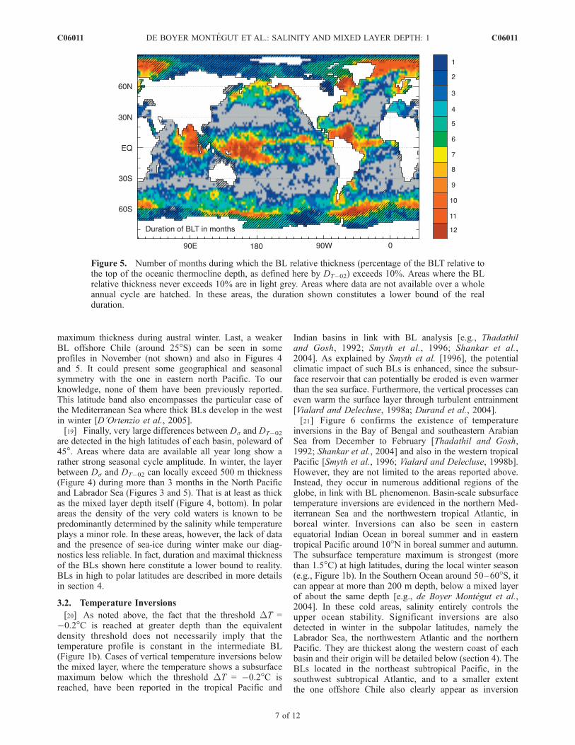
Figure 5. Number of months during which the BL relative thickness (percentage of the BLT relative tothe top of the oceanic thermocline depth, as defined here by DT�02) exceeds 10%. Areas where the BLrelative thickness never exceeds 10% are in light grey. Areas where data are not available over a wholeannual cycle are hatched. In these areas, the duration shown constitutes a lower bound of the realduration.


7 of 12

C06011

Figure 6. (a) Amplitude, (b) depth, and (c) month of the annual maximal temperature inversionsdetected in the profiles below the mixed layer. More than 3 million profiles from 1967 to 2006 were usedto compute those inversions (see Figure 2b). In order to study reliable inversion patterns, we computemaximal inversions by considering only monthly grid points with at least five available individualprofiles and where more than 25% of those profiles exhibit an inversion of at least 0.2�C. Note thatkriging was not applied to obtain these maps in order to only detect single profiles presenting aninversion.


8 of 12

C06011

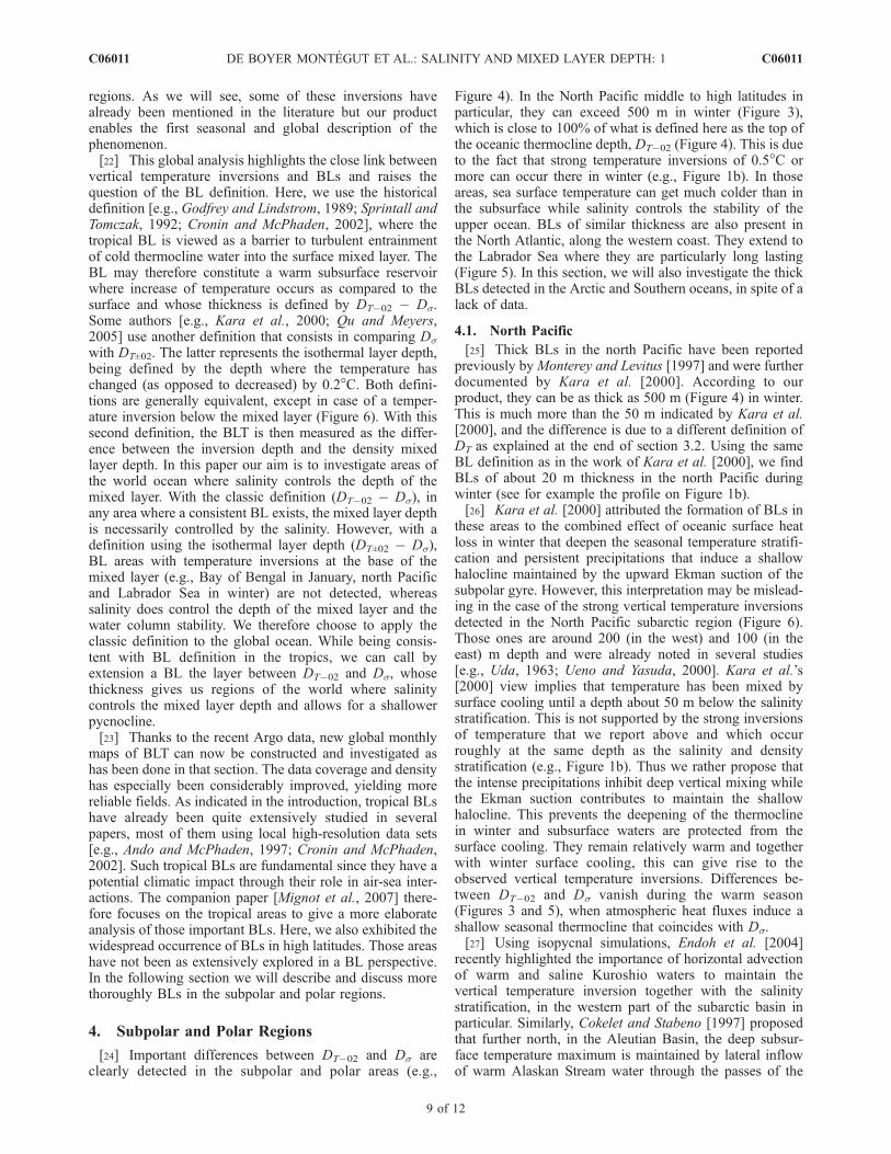
regions. As we will see, some of these inversions havealready been mentioned in the literature but our productenables the first seasonal and global description of thephenomenon.[22] This global analysis highlights the close link between

vertical temperature inversions and BLs and raises thequestion of the BL definition. Here, we use the historicaldefinition [e.g., Godfrey and Lindstrom, 1989; Sprintall andTomczak, 1992; Cronin and McPhaden, 2002], where thetropical BL is viewed as a barrier to turbulent entrainmentof cold thermocline water into the surface mixed layer. TheBL may therefore constitute a warm subsurface reservoirwhere increase of temperature occurs as compared to thesurface and whose thickness is defined by DT�02 � Ds.Some authors [e.g., Kara et al., 2000; Qu and Meyers,2005] use another definition that consists in comparing Dswith DT±02. The latter represents the isothermal layer depth,being defined by the depth where the temperature haschanged (as opposed to decreased) by 0.2�C. Both defini-tions are generally equivalent, except in case of a temper-ature inversion below the mixed layer (Figure 6). With thissecond definition, the BLT is then measured as the differ-ence between the inversion depth and the density mixedlayer depth. In this paper our aim is to investigate areas ofthe world ocean where salinity controls the depth of themixed layer. With the classic definition (DT�02 � Ds), inany area where a consistent BL exists, the mixed layer depthis necessarily controlled by the salinity. However, with adefinition using the isothermal layer depth (DT±02 � Ds),BL areas with temperature inversions at the base of themixed layer (e.g., Bay of Bengal in January, north Pacificand Labrador Sea in winter) are not detected, whereassalinity does control the depth of the mixed layer and thewater column stability. We therefore choose to apply theclassic definition to the global ocean. While being consis-tent with BL definition in the tropics, we can call byextension a BL the layer between DT�02 and Ds, whosethickness gives us regions of the world where salinitycontrols the mixed layer depth and allows for a shallowerpycnocline.[23] Thanks to the recent Argo data, new global monthly

maps of BLT can now be constructed and investigated ashas been done in that section. The data coverage and densityhas especially been considerably improved, yielding morereliable fields. As indicated in the introduction, tropical BLshave already been quite extensively studied in severalpapers, most of them using local high-resolution data sets[e.g., Ando and McPhaden, 1997; Cronin and McPhaden,2002]. Such tropical BLs are fundamental since they have apotential climatic impact through their role in air-sea inter-actions. The companion paper [Mignot et al., 2007] there-fore focuses on the tropical areas to give a more elaborateanalysis of those important BLs. Here, we also exhibited thewidespread occurrence of BLs in high latitudes. Those areashave not been as extensively explored in a BL perspective.In the following section we will describe and discuss morethoroughly BLs in the subpolar and polar regions.

4. Subpolar and Polar Regions

[24] Important differences between DT�02 and Ds areclearly detected in the subpolar and polar areas (e.g.,

Figure 4). In the North Pacific middle to high latitudes inparticular, they can exceed 500 m in winter (Figure 3),which is close to 100% of what is defined here as the top ofthe oceanic thermocline depth, DT�02 (Figure 4). This is dueto the fact that strong temperature inversions of 0.5�C ormore can occur there in winter (e.g., Figure 1b). In thoseareas, sea surface temperature can get much colder than inthe subsurface while salinity controls the stability of theupper ocean. BLs of similar thickness are also present inthe North Atlantic, along the western coast. They extend tothe Labrador Sea where they are particularly long lasting(Figure 5). In this section, we will also investigate the thickBLs detected in the Arctic and Southern oceans, in spite of alack of data.

4.1. North Pacific

[25] Thick BLs in the north Pacific have been reportedpreviously byMonterey and Levitus [1997] and were furtherdocumented by Kara et al. [2000]. According to ourproduct, they can be as thick as 500 m (Figure 4) in winter.This is much more than the 50 m indicated by Kara et al.[2000], and the difference is due to a different definition ofDT as explained at the end of section 3.2. Using the sameBL definition as in the work of Kara et al. [2000], we findBLs of about 20 m thickness in the north Pacific duringwinter (see for example the profile on Figure 1b).[26] Kara et al. [2000] attributed the formation of BLs in

these areas to the combined effect of oceanic surface heatloss in winter that deepen the seasonal temperature stratifi-cation and persistent precipitations that induce a shallowhalocline maintained by the upward Ekman suction of thesubpolar gyre. However, this interpretation may be mislead-ing in the case of the strong vertical temperature inversionsdetected in the North Pacific subarctic region (Figure 6).Those ones are around 200 (in the west) and 100 (in theeast) m depth and were already noted in several studies[e.g., Uda, 1963; Ueno and Yasuda, 2000]. Kara et al.’s[2000] view implies that temperature has been mixed bysurface cooling until a depth about 50 m below the salinitystratification. This is not supported by the strong inversionsof temperature that we report above and which occurroughly at the same depth as the salinity and densitystratification (e.g., Figure 1b). Thus we rather propose thatthe intense precipitations inhibit deep vertical mixing whilethe Ekman suction contributes to maintain the shallowhalocline. This prevents the deepening of the thermoclinein winter and subsurface waters are protected from thesurface cooling. They remain relatively warm and togetherwith winter surface cooling, this can give rise to theobserved vertical temperature inversions. Differences be-tween DT�02 and Ds vanish during the warm season(Figures 3 and 5), when atmospheric heat fluxes induce ashallow seasonal thermocline that coincides with Ds.[27] Using isopycnal simulations, Endoh et al. [2004]

recently highlighted the importance of horizontal advectionof warm and saline Kuroshio waters to maintain thevertical temperature inversion together with the salinitystratification, in the western part of the subarctic basin inparticular. Similarly, Cokelet and Stabeno [1997] proposedthat further north, in the Aleutian Basin, the deep subsur-face temperature maximum is maintained by lateral inflowof warm Alaskan Stream water through the passes of the


9 of 12

C06011

Aleutian Basin. Beside that basin, the eastern North Pacificwinter BL might be linked with the formation of easternNorth Pacific Subtropical Mode Waters, which is subjectto strong interannual variability compared to other modewaters. More analysis is needed to quantify the respectiverole of the local and the advective mechanism. Note yetthat in both cases, the Ekman suction of the subpolar gyreplays an important role in maintaining the halocline andthe vertical temperature inversion. Note also that Wirts andJohnson [2005] recently reported that the subsurfacetemperature inversion of the southeast Aleutian Basinhad decreased during the last winters due to a combinationof atypical ocean advection and anomalous atmosphericforcing. This should correspond to modifications of the BLpattern.

4.2. North Atlantic

[28] Thick BLs in the western Atlantic midlatitudes (40–55�N) have never been mentioned or described to ourknowledge. They are confined to the shelfbreak of theMiddle Atlantic Bight, along the eastern American coastsouth of Newfoundland (Figure 3). The situation looks verysimilar to its Pacific counterpart, although the BLs are quitethinner (up to about 100 m, Figures 3 and 4, top) and theydo not extend eastward across the basin. Inversions are alsopresent but they are shallower (Figure 6). They are even asshallow as 20 to 40 m in the south of the area, in a smallzone north of Cape Hatteras, consistent with Linder andGawarkiewicz’s [1998] findings.[29] The area along the American coast, following the

path of the Gulf Stream, constitutes a boundary between thecool, fresh continental shelf water mass and the warm,saline so-called ‘‘upper slope water pycnostad’’ [Wrightand Parker, 1976; Linder and Gawarkiewicz, 1998] below,which results from the complex interaction of the GulfStream with local waters [e.g., Pickart et al., 1999]. Thissuperposition of different water masses is the origin of theinversed vertical temperature profiles (Figure 6), which arehere again partly maintained by upward Ekman pumping(not shown) and the positive buoyancy flux inhibitingvertical mixing. The high SSS values of the North Atlanticand its specific circulation are probably the reason why theBL does not extends eastward as much as in the Pacific.[30] It is not clear whether similar BLs are present also in

the Southern Hemisphere. A BL of about 30 m thickness ispresent in austral winter (July to September) in the westernSouth Atlantic (35�S–50�W, Figure 3). It also presents asignificant temperature inversion (Figure 6) and could thusbe symmetrical to the ones detected in the Northern Hemi-sphere. No equivalent is yet detected in the other basins.

4.3. Arctic Ocean and Nordic and Labrador Seas

[31] In the Arctic ocean the surface mixed layer is veryfresh, as a result of precipitation and abundant river dis-charges [e.g., Aagaard and Carmack, 1989], with a tem-perature virtually at the freezing point. The water mass thatlies below consists of warm and salty Atlantic waters thatenter the Eurasian Basin through Fram Strait and across theBarents Sea [e.g., Rudels et al., 1996; Morison et al., 1998].In all seasons but summer, a strong halocline thus definesDs while below, the temperature profile is again typicallyunstable, as shown in Figure 6. Note that this halocline is

relatively thick and influenced, among other, by the sea-sonal inflow of relatively fresh Pacific waters throughBering Strait [e.g., Woodgate et al., 2005]. In summer,atmospheric heating over open water and leads induces ashallow seasonal thermocline that limits the warmed mixedlayer. The difference in density and temperature stratifica-tion is thus strongly reduced (Figure 3, compare JAS andOND). Lack of data might however introduce biases in theresults in this area.[32] The winter situation in the Baltic Sea, where warm

and salty waters from the Atlantic penetrate through irreg-ular pulses under the fresh surface layer, resulting in a sharppermanent halocline around 50 to 80 m depth [e.g., Meier,2001], is similar to the Arctic Ocean. In summer, atmo-spheric heating is such that no more stratification is detectedby our criteria. In the Labrador and Nordic Seas, as well asin the Bering Sea, the winter vertical stratification is verysimilar to that of the Arctic ocean and temperature inver-sions are also present (Figure 6).

4.4. Austral Ocean

[33] Thickest differences between DT�02 and Ds arefinally detected in the Austral Ocean southward of the polarfront (about 54�S) in austral winter (Figure 3 and 4). Theyare also associated to the largest and deepest verticaltemperature inversions (Figure 6). The deep and cold layerof Winter Water is indeed overlying the warmer and saltierUpper Circumpolar Deep Water [e.g., Rintoul et al., 2001]inducing a situation symmetrical to that of the extremenorth. From the analysis of several sections between Tas-mania and Antarctica, Chaigneau et al. [2004] confirmedthat the salinity maintains the stability of the water columnwhich would otherwise be destabilized by a 3�C tempera-ture drop across the mixed layer. In summer the warmerAntarctic Surface Water defines a shallow thermocline thatlimits the mixed layer depth [Chaigneau et al., 2004]. Dsand DT�02 are then equal.

5. Conclusions

[34] We have presented and analyzed a new climatology ofthe differences between temperature and density stratifica-tion in the upper ocean highlighting the influence of salinityon this stratification. The product is based on the compilationof the recent NODC,WOCE, and Argo databases. The use ofthe latter in particular represents a substantive improvementwith respect to de Boyer Montegut et al.’s [2004] preliminaryresults in terms of BL analysis. It leads to a considerableincrease in data coverage and density, representing 30% ofthe total profiles of the data. The main novelty of ourclimatology as compared to previous global and large-scalestudies is that it is based on profile-wise computations. Thisresults in more realistic and detailed structures than alreadygridded profiles, since no merging by smoothing or interpo-lation is applied.[35] Generally, the analysis has confirmed that the classic

picture of temperature and salinity being mixed over thesame depth is highly simplified. In the real ocean thesituation is very often different. Quasi-permanent (10–12 months) BLs are observed in the equatorial and westerntropical Pacific and Atlantic, in the Bay of Bengal and theeastern equatorial Indian Ocean, in the Labrador Sea, and


10 of 12

C06011

parts of the Arctic and Southern Ocean. In the northernAtlantic and Pacific subpolar basins, in the southern IndianOcean, in the Arabian Sea, and equatorward of the subtrop-ical Atlantic and Pacific salinity maxima, BLs are ratherseasonal, lasting about 6 months per year. BLs are finallyalmost never detected around 30–40� of latitude in eachbasin and in tropical and subtropical coastal upwellingregions, where mixed layers are extremely shallow. Oneimportant exception is, however, the BL in the Java andSumatra area which has been extensively studied byMassonet al. [2002] and Qu and Meyers [2005].[36] These BLs patterns are often associated with tem-

perature inversions below the homogeneous surface layer.The latter may exist since salinity controls the stratificationand water column stability in the upper ocean. Suchinversions occur in several regions of the globe. In thetropics the most striking ones are in the Bay of Bengal andsoutheastern Arabian Sea in winter, in the west tropicalPacific, in the east equatorial Indian Ocean, and a largepattern in the northwestern tropical Atlantic during winter.Temperature inversions are maximum in amplitude anddepth (reaching more than 1.5�C at depth over 100 m) inhigh latitudes in winter (e.g., north Pacific, Southern Ocean,Labrador Sea).[37] Poleward of about 45�N and S, winter vertical

temperature profiles are very often inversed, i.e., the tem-perature is maximum below the mixed layer, around 100 tomore than 200 m depth (austral Ocean). Inversions areparticularly deep and strong along the eastern coast, in theKuroshio (Pacific) and Gulf Stream (Atlantic) path. Thisresults in thick (up to about 500 m in the northwesternPacific) differences between Ds and DT�02 in the NorthPacific and western Atlantic in winter. These differenceshave already been reported recently [Kara et al., 2000], butthe characteristic temperature inversions was not discussed.[38] That phenomenon enabled us to propose a slightly

different formation mechanism than the one proposed bythese authors. It implies the formation of a persistenthalocline by intense precipitation, partly maintained byEkman succion, that prevents the surface cooling to pene-trate at depth. Moreover, regarding the temperature inver-sion, subsurface advection by the western boundary currentand their open ocean drift of warmer and saltier water thanthe surface might also contribute to the observed structure inboth basins. Note that while these BLs are located across thewhole basin in the Pacific, they are slightly thinner andrather confined to the western basin in the Atlantic. Max-imum temperature inversions are also shallower.[39] In the Southern Ocean, the maximal subsurface

temperature inversion can exceed 1.5�C compared to thesurface and be reached around 250 m depth. Generally, inthe polar areas, the density and the stability of the upperocean are primarily controlled by the salinity. The temper-ature inversions are due to the presence of a very fresh andrelatively cold surface layer that lies above a warmer andsaltier water mass advected from equatorward areas. Coldwinter atmospheric fluxes but also intense input of fresh-water from the atmospheric precipitations (Arctic andsouthern oceans) or river runoff (Arctic ocean) thus play amajor role in setting this vertical structure. In summer theseasonal thermocline resulting from surface heating gener-ally limits the mixed layer depth, and the BL disappears.

The latter can however persist several months in areas thatare still covered with ice (open Arctic ocean) and in areaswhere very fresh surface waters induced by sea ice meltingin late winter-early spring prevent the warming of thesubsurface waters (Labrador and Nordic Seas, area of theBering Strait).[40] Our concern was not to assess each BL formation

mechanism in details. We believe that this should be doneultimately by different groups, focusing on specific areas.The present analysis suggests that these mechanisms arevarious and often not simple, implying atmospheric fresh-water and heat forcing, advection, and runoff. Yet, asymmetry in terms of BL occurrence, seasonality, andformation mechanism has been revealed for the subpolarNorth Pacific and western Atlantic and for the polar regions.The companion paper [Mignot et al., 2007] shows that thisholds also for the BLs located immediately equatorward ofthe salinity subtropical maximum. Finally this north-southhemispheres symmetry appears to be true at any latitudeaway from the deep tropics.[41] Our global analysis has provided some new under-

standing of the BL formation mechanism in areas such asthe northern Atlantic and Pacific basin. However, the differ-ences between the northern Atlantic and Pacific oceans hasto be investigated in greater details together with thequantification of the advective versus the local mechanism.[42] Finally, the origin of BLs detected in the 25–45�

latitude zone (offshore California, Rio de la Plata, andChile) and associated to vertical temperature inversionswere not explained. To our knowledge, it is not referredin the literature, but it corresponds to a well covered areaand should thus be robust. Future work should be dedicatedto their understanding.[43] We also detected significant large-scale areas where a

vertical compensation between salinity and temperaturestratification occurs. They seem to be detected primarilyin winter and in the midlatitudes of each basins and theirthickness is significant in comparison to the mixed layerdepth in the southern ocean, equatorward of the subpolarfront, and in the North Atlantic. They will be investigated indetails in a forthcoming study.[44] The structures and orders of magnitude that we

detected are overall in agreement with previous large-scalestudies [Sprintall and Tomczak, 1992; Tomczak and Godfrey,1994; Monterey and Levitus, 1997] and more detailed localstudies (several references in the text). We believe that thedata set would be useful for a large spectrum of oceano-graphic studies such as the revision of accurate upper oceanheat, salt, and biological budgets, and the validation of oceangeneral circulation models. In several regions, mechanismsof BL formation and destruction are indeed still poorlyunderstood. Owing to the lack of data, their investigationrequires the use of ocean general circulation models, thatneed to be validated against a reliable and robust product[e.g., Durand et al., 2007]. For these reasons, we would liketo make our product public. The monthly mean differencesDT�02 � Ds as well as the fields DT�02 and Ds themselvescan be downloaded from http://www.locean-ipsl.upmc.fr/�cdblod/blt.html.

[45] Acknowledgments. We would like to acknowledge the NationalOceanographic Data Center, the World Ocean Circulation Experiment, and


11 of 12

C06011

the Coriolis project for the rich publicly available databases. We are gratefulto Gilles Reverdin for stimulating discussions, constructive comments, andencouragements and to Fabien Durand and Roger Lukas for detailedcomments on the manuscript. We also thank the anonymous reviewersfor their constructive comments that lead to the improvements of themanuscript. CBM was partly supported by a DGA grant (DGA-CNRS2001292) and by fundings of the Programme National d’Etude de laDynamique et du Climat (PNEDC).

ReferencesAagaard, K., and E. Carmack (1989), The role of sea ice and other freshwater in the arctic circulation, J. Geophys. Res., 94, 14,485–14,497.

Ando, K., and M. J. McPhaden (1997), Variability of surface layerhydrography in the tropical Pacific Ocean, J. Geophys. Res., 102,23,063–23,078.

Chaigneau, A., R. A. Morrow, and S. R. Rintoul (2004), Seasonal andinterannual evolution of the mixed layer in the Antarctic Zone south ofTasmania, Deep Sea Res. I, 51, 2047–2072.

Cokelet, E. D., and P. J. Stabeno (1997), Mooring, observations of thethermal structure, salinity and currents in the SE Bering Sea basin,J. Geophys. Res., 102, 22,947–22,964.

Cronin, M. F., and M. J. McPhaden (2002), Barrier layer formation duringwesterly wind bursts, J. Geophys. Res., 107(C12), 8020, doi:10.1029/2001JC001171.

de Boyer Montegut, C., G. Madec, A. S. Fisher, A. Lazar, and D. Iudicone(2004), Mixed layer depth over the global ocean: an examination ofprofile data and a profile-based climatology, J. Geophys. Res., 109,C12003, doi:10.1029/2004JC002378.

Defant, A. (1961), Physical Oceanography, vol. 1, 729 pp., Pergamon,London.

D’Ortenzio, F., D. Iudicone, C. de Boyer Montegut, P. Testor, D. Antoine,S. Marullo, R. Santoleri, and G. Madec (2005), Seasonal variability of themixed layer depth in the Mediterranean Sea as derived from in situprofiles, Geophys. Res. Lett., 32, L12605, doi:10.1029/2005GL022463.

Durand, F., S. R. Shetye, J. Vialard, D. Shankar, S. S. C. Shenoi, C. Ethe,and G. Madec (2004), Impact of temperature inversion on SST evolutionin the South-Eastern Arabian Sea during the pre-summer monsoon sea-son, Geophys. Res. Lett., 31, L01305, doi:10.1029/2003GL018906.

Durand, F., D. Shankar, C. de Boyer Montegut, S. S. C. Shenoi, B. Blanke,and G. Madec (2007), Modeling the barrier-layer formation in the South-Eastern Arabian Sea, J. Clim, 20, 2109–2120.

Endoh, T., H. Mitsudera, S.-P. Xie, and B. Qiu (2004), Thermohalinestructure in the subarctic North Pacific simulated in a general circulationmodel, J. Phys. Oceanogr., 34, 360–371.

Godfrey, J. S., and E. J. Lindstrom (1989), The heat budget of the equatorialwestern Pacific surface mixed layer, J. Geophys. Res., 94, 8007–8017.

Kara, A. B., P. A. Rochford, and H. E. Hulburt (2000), Mixed layer depthvariability and barrier layer formation over the North Pacific Ocean,J. Geophys. Res., 105, 16,803–16,821.

Levitus, S. (1982), Climatological atlas of the world ocean, tech. rep. 13,NOAA, Rockville, Md.

Levitus, S., and T. Boyer (1994), Temperature, vol. 4, World Ocean Atlas,117 pp., NOAA, Washington D. C.

Lindstrom, E., R. Lukas, R. Fine, E. Firing, S. Godfrey, G. Meyers, andM. Tsuchiya (1987), The Western Equatorial Pacific Ocean CirculationStudy, Nature, 300, 533–537.

Linder, C. A., and G. Gawarkiewicz (1998), A climatology of the shelf-break front in the Middle Atlantic Bight, J. Geophys. Res., 103,18,405–18,423.

Lozier, M. S., M. S. McCartney, and W. B. Owens (1994), Anomalousanomalies in averaged hydrographic data, J. Phys. Oceanogr., 24,2624–2638.

Lukas, R., and E. Lindstrom (1987), The mixed layer of the western equa-torial Pacific Ocean, paper presented at ‘Aha Huliko’a Hawaiian WinterWorkshop on the Dynamics of the Oceanic Surface Mixed Layer, HawaiiInst. of Geophys., Honolulu.

Lukas, R., and E. Lindstrom (1991), The mixed layer of the western equa-torial Pacific Ocean, J. Geophys. Res., 96, 3343–3357.

Maes, C., J. Picaut, and S. Belamari (2002), Salinity barrier layer and onsetof El Nino in a Pacific coupled model, Geophys. Res. Lett., 29(24), 2206,doi:10.1029/2002GL016029.

Maes, C., J. Picaut, A. Kentaro, and K. Yoshifumi (2004), Characteristics ofthe convergence zone at the eastern edge of the Pacific warm pool,Geophys. Res. Lett., 31, L11304, doi:10.1029/2004GL019867.

Masson, S., P. Delecluse, J.-P. Boulager, and C. Menkes (2002), A modelstudy of the seasonal variability and formation mechanisms of the barrierlayer in the equatorial Indian Ocean, J. Geophys. Res., 107(C12), 8017,doi:10.1029/2001JC000832.

Masson, S., J.-J. Luo, G.Madec, J. Vialard, F. Durand, S. Gualdi, E. Guilyardi,S. Behera, P. Delecluse, A. Navarra, and P. Yamagata (2005), Impact of

barrier layer on winterspring variability of the southeastern Arabian Sea,Geophys. Res. Lett., 32, L07703, doi:10.1029/2004GL021980.

Meier, H. E. M. (2001), On the parameterization of mixing in 3D Baltic Seamodels, J. Geophys. Res., 106, 30,997–31,016.

Mignot, J., C. de Boyer Montegut, A. Lazar, and S. Cravatte (2007),Control of salinity on the mixed layer depth in the world ocean: 2.Tropical areas, J. Geophys. Res., doi:10.1029/2006JC003954, in press.

Monterey, G., and S. Levitus (1997), Seasonnal variability of mixed layerdepth for the world ocean, technical report, NOAA, Silver Spring, Md.

Morison, J., M. Steele, and R. Anderson (1998), Hydrography of the upperArctic Ocean measured from the nuclear submarine USS Pargo, Deep SeaRes. I, 45, 15–38.

Pickart, R. S., T. K. McKee, D. J. Torres, and S. A. Harrington (1999),Mean structure and variability of the slopewater system south of New-foundland, J. Phys. Oceanogr., 29, 2541–2558.

Qu, T., and G. Meyers (2005), Seasonal variation of barrier layer in thesoutheastern tropical Indian Ocean, J. Geophys. Res., 110, C11003,doi:10.1029/2004JC002816.

Reverdin, G., D. Cayan, and Y. Kushnir (1997), Decadal variabilityof hydrography in the upper northern North Atlantic in 1948–1990,J. Geophys. Res., 102, 8505–8531.

Rintoul, S. R., C. W. Hughes, and D. Olbers (2001), The Antarctic Cir-cumpolar Current system, in Ocean Circulation and Climate, edited byG. Siedler,W. J.Gould, and J. Church, pp. 271–301,Academic,NewYork.

Rotschi, H., P. Hisard, and F. Jarrige (1972), Les eaux du Pacifique occidentala 170E entre 20S et 4N, technical report, Inst. de Rech. pour le Dev., Paris.

Rudels, B., L. G. Anderson, and E. P. Jones (1996), Formation andevolution of the surface mixed layer and halocline of the Arctic Ocean,J. Geophys. Res., 101, 8807–8821.

Sato, K., T. Suga, and K. Hanawa (2004), Barrier layer in the North Pacificsubtropical gyre, Geophys. Res. Lett., 31, L05301, doi:10.1029/2003GL018590.

Shankar, D., V. V. Gopalakrishna, S. S. C. Shenoi, F. Durand, S. R. Shetye,C. K. Rajan, Z. Johnson, N. Araligidad, and G. S. Michael (2004), Ob-servational evidence for westward propagation of temperature inversionin the southeastern Arabian Sea, Geophys. Res. Lett., 31, L08305,doi:10.1029/2004GL019652.

Smyth, W. D., D. Hebert, and J. N. Moum (1996), Local ocean response toa multiphase westerly wind burst: 2. Thermal and freshwater responses,J. Geophys. Res., 101, 22,513–22,534.

Sprintall, J., and M. Tomczak (1992), Evidence of the barrier layer in thesurface layer of the Tropics, J. Geophys. Res., 97, 7305–7316.

Stommel, H., and K. N. Fedorov (1967), Small scale structure in tempera-ture and salinity near Timor and Mindanao, Tellus, 19, 306–325.

Thadathil, P., and A. K. Gosh (1992), Surface layer temperature inversion inthe Arabian Sea during winter, J. Oceanogr., 48, 293–304.

Tomczak, M., and J. S. Godfrey (1994), Regional Oceanography: AnIntroduction, Pergamon, New York. (Avalaible at http://www.cmima.csic.es/mirror/mattom/regoc/pdfversion.html)

Uda, M. (1963), Oceanography of the Subarctic Pacific Ocean, J. Fish. Res.Board Can., 20, 119–179.

Ueno, H., and I. Yasuda (2000), Distribution and formation of the mesother-mal structure (temperture inversions) in the North Pacific subarctic region,J. Geophys. Res., 105, 16,885–16,897.

Vialard, J., and P. Delecluse (1998a), An OGCM study for the TOGAdecade. part 1: role of salinity in the physics of the western Pacific freshpool, J. Phys. Oceanogr., 28, 1071–1088.

Vialard, J., and P. Delecluse (1998b), An OGCM study for the TOGAdecade. part 2: barrier-layer formation and variability, J. Phys. Oceanogr.,28, 1089–1106.

Wirts, A. E., and G. C. Johnson (2005), Recent interannual upper oceanvariability in the deep southeastern Bering Sea, J. Mar. Res., 63, 381–405.

Woodgate, R. A., K. Aagaard, and T. J. Weingartner (2005), Monthlytemperature, salinity, and transport variability of the Bering Strait throughflow, Geophys. Res. Lett., 32, L04601, doi:10.1029/2004GL021880.

Wright, W. R., and C. E. Parker (1976), A volumetric temperature/salinitycensus for the Middle Atlantic Bight, Limnol. Oceanogr., 21, 563–571.

��S. Cravatte, Laboratoire d’Etudes en Geophysique et Oceanographie

Spatiales, Unite Mixte de Recherche, CNRS/IRD/CNES/Universite PaulSabatier, 14, av. Edouard Belin, F-31400 Toulouse, France.A. Lazar and J. Mignot, Laboratoire d’Oceanographie et du Climat:

Experimentations et Approches Numeriques, Institut Pierre Simon Laplace,Unite Mixte de Recherche, CNRS/IRD/UPMC, 4 place Jussieu, Case 100,F-75252 Paris, France.C. de Boyer Montegut, Frontier Research Center for Global Change,

Japan Agency for Marine-Earth Science and Technology, 3173-25 Showa-machi, Kanazawa-ku, Yokohama, Kanagawa 236-0001 Japan.


12 of 12

C06011

control of salinity on the mixed layer depth in the world ocean: 1...

Documents