WATER RESOURCES RESEARCH, VOL. ???, XXXX, DOI:10.1002/,

Control of Water Distribution Networks with1

Dynamic DMA Topology Using Strictly Feasible2

Sequential Convex Programming3

Robert Wright1, Edo Abraham

1, Panos Parpas

2, Ivan Stoianov

1

Corresponding author: Robert Wright, InfraSense Labs, Dept. of Civil and Environmental

Eng., Imperial College London, SW7 2BU, London, UK. (robert.wright07@imperial.ac.uk)

1InfraSense Labs, Dept. of Civil and

Environmental Eng., Imperial College

London SW7 2BU, London, UK.

2Dept. of Computing, Imperial College

London SW7 2BU, London, UK.

D R A F T October 9, 2015, 5:52pm D R A F T

X - 2 WRIGHT ET AL.: WATER DISTRIBTUION NETWORKS WITH DYNAMIC TOPOLOGY

Abstract. The operation of water distribution networks (WDN) with a4

dynamic topology is a recently pioneered approach for the advanced man-5

agement of district metered areas (DMA) that integrates novel developments6

in hydraulic modelling, monitoring, optimization and control. A common prac-7

tice for leakage management is the sectorization of WDNs into small zones,8

called DMAs, by permanently closing isolation valves. This facilitates wa-9

ter companies to identify bursts and estimate leakage levels by measuring10

the inlet flow for each DMA. However, by permanently closing valves, a num-11

ber of problems have been created including reduced resilience to failure and12

suboptimal pressure management. By introducing a dynamic topology to these13

zones, these disadvantages can be eliminated whilst still retaining the DMA14

structure for leakage monitoring. In this paper, a novel optimization method15

based on sequential convex programming (SCP) is outlined for the control16

of a dynamic topology with the objective of reducing average zone pressure17

(AZP). A key attribute for control optimization is reliable convergence. To18

achieve this, the SCP method we propose guarantees that each optimization19

step is strictly feasible, resulting in improved convergence properties. By us-20

ing a null space algorithm for hydraulic analyses, the computations required21

are also significantly reduced. The optimized control is actuated on a real22

WDN operated with a dynamic topology. This unique experimental programme23

incorporates a number of technologies set up with the objective of investi-24

gating pioneering developments in WDN management. Preliminary results25

D R A F T October 9, 2015, 5:52pm D R A F T

WRIGHT ET AL.: WATER DISTRIBTUION NETWORKS WITH DYNAMIC TOPOLOGY X - 3

indicate AZP reductions for a dynamic topology of up to 6.5% over optimally26

controlled fixed topology DMAs.27

D R A F T October 9, 2015, 5:52pm D R A F T

X - 4 WRIGHT ET AL.: WATER DISTRIBTUION NETWORKS WITH DYNAMIC TOPOLOGY

KeyWords Dynamic Topology, Water Distribution Networks, Optimization, Pressure28

Management, Flow Modulation29

30

1. Introduction

The installation of District Metered Areas (DMA) is one of the most successful methods31

that water companies use for identifying and reducing leakage and implementing simplistic32

pressure management. This involves the segregation of the water distribution network33

(WDN) into small zones, known as DMAs, by permanently closing isolation valves. Their34

permanent closure stops flow from breaching the boundary of the DMA and they are35

therefore commonly referred to as boundary valves (BV). Each DMA typically has a36

single inlet (feed). The benefits of this approach are as follows:37

During times of low demand (i.e. at night), the flow at the DMA inlet is monitored38

and leakage estimates are made. This aids in the identification of new bursts as well39

as prioritization within rehabilitation schemes for DMAs that possess high background40

leakage.41

Simplistic pressure management can be implemented by installing a pressure reducing42

valve (PRV) at the DMA inlet. Reducing the average zone pressure (AZP) reduces leakage43

within the DMA. The pressure reduction must be carried out with a high degree of44

certainty to ensure customers still receive an adequate level of service i.e. a minimum45

allowable pressure must be maintained. In order to aid with this, a water company can46

monitor pressure at the critical point (CP) of the DMA, which is defined as the point of47

the DMA where pressure is closest to the minimum allowable pressure. Provided that the48

CP of the DMA does not move, maintaining a minimum allowable pressure at the CP49

D R A F T October 9, 2015, 5:52pm D R A F T

WRIGHT ET AL.: WATER DISTRIBTUION NETWORKS WITH DYNAMIC TOPOLOGY X - 5

guarantees that all customers in the DMA have a sufficient level of service. There is also50

substantial evidence that pressure management reduces future burst frequency (Lalonde51

et al. [2008] and Fantozzi et al. [2009] report burst reductions of up to 40% following the52

implementation of pressure management).53

The implementation of DMAs in the UK has successfully facilitated water companies54

to reduce leakage by 30% over the last 25 years [Ofwat , 2007]. Its implementation how-55

ever has not been without several severe drawbacks due to the permanent closure of the56

boundary valves, and are summarized as follows:57

Reduced resilience to failure. In this paper, we use redundancy as a measure of resilience58

to failure [Yazdani et al., 2011]. The permanent closure of boundary valves reduces the59

network redundancy which results in a reduced number of independent supply routes60

for consumers. The network is therefore less resilient to failure. For single feed DMAs,61

more single points of failure exist. In the event of failure, boundary valves are commonly62

opened manually in order to sustain pressure and keep customers in service [Drinking63

Water Inspectorate, 2009]. The manual opening of boundary valves must be undertaken64

carefully to avoid the generation of pressure transients that could cause secondary pipe65

failures. Furthermore, a substantial amount of time is needed to detect the incident, plan66

a rezone of the DMA, and travel to the affected area in order to open boundary valves,67

during which time the customers service is disrupted.68

Suboptimal pressure management due to higher frictional energy losses occurring in single69

feed DMAs [Wright et al., 2014]. By operating a DMA with multiple sources, new paths70

exist between demand nodes and source nodes. This increased redundancy generally71

results in lower frictional energy losses due to the principle of least action [Piller et al.,72

D R A F T October 9, 2015, 5:52pm D R A F T

X - 6 WRIGHT ET AL.: WATER DISTRIBTUION NETWORKS WITH DYNAMIC TOPOLOGY

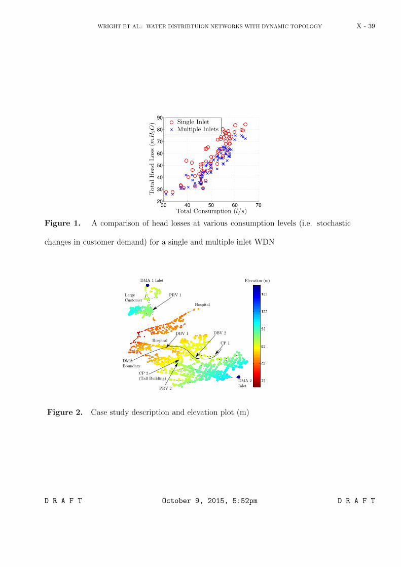
2003]. Figure 1 demonstrates this process. The total frictional head losses in a WDN73

model are summed and plotted with the corresponding total instantaneous consumption.74

Two scenarios are tested, the first has a single source available, and the second has two75

sources available. All other aspects of the WDN model are identical. The head losses76

are on average 12.7% lower for the WDN with multiple sources. PRVs can consequently77

operate with a lower outlet pressure that still maintains pressure at the CP of the network,78

which is facilitated by the reduction in frictional head losses.79

Water quality incidents due to the build-up of stagnant water at artificially created80

dead ends [World Health Organization, 2004]. This problem is exacerbated when the81

closed boundary valves need to be opened, such as failure events. This can lead to the82

customers water supply becoming discolored and penalties issued by the regulator. The83

World Health Organization [2004] recommends that the artificial implementation of dead84

ends is limited in the design and operation of WDNs.85

The disadvantages of implementing DMAs are now becoming more detrimental as water86

companies in the UK are facing severe financial penalties for poor customer service from87

the economic regular, known as Ofwat. These penalties fall under service frameworks such88

as the Service Incentive Mechanism (SIM, Ofwat [2012]) and the Guaranteed Standards89

Scheme (GSS, Ofwat [2008]). The size of the penalties can be as high as 1% of the water90

companys revenue [Ofwat , 2014]. Instances of poor customer service range from low91

pressures (GSS Regulation 10), stagnant or discoloured water at the customers supply92

point [Drinking Water Inspectorate, 2009], supply failure (GSS Regulation 8 and 9) as93

well as customers needing to contact their water companies for other reasons related94

to their service, which they may consider to be unsatisfactory. One example of this is95

D R A F T October 9, 2015, 5:52pm D R A F T

WRIGHT ET AL.: WATER DISTRIBTUION NETWORKS WITH DYNAMIC TOPOLOGY X - 7

high variability in diurnal pressure, which affects the perception of a good level of service96

(personal communications with water companies). Furthermore, water companies are also97

rewarded up to 0.5% of their revenue for performing well in the SIM framework [Ofwat ,98

2014], adding further incentive to provide a strong level of service. In order to address these99

new requirements in customer service levels, utilities need to carefully plan mitigations100

that are also closely linked with addressing the disadvantages of DMAs. Finally, there is101

still a strong emphasis being placed on further reducing leakage levels.102

DMAs with dynamic topology is a novel approach to the operational management of103

WDNs, where DMAs are dynamically aggregated for improved network resilience, pres-104

sure management and water quality, and segregated periodically (e.g. each night, once105

per week, etc.) for leakage monitoring at night [Wright et al., 2014]. This is facilitated106

by replacing certain closed boundary valves with self-powered, remote control valves, i.e.107

dynamic boundary valves (DBV), that incorporate a novel dual bypass pilot system for108

bidirectional flow and control. The operation of a dynamic DMA topology can therefore109

successfully eliminates the disadvantages of conventional DMAs, whilst retaining or even110

improving its success in leakage monitoring, since even smaller DMAs can be set up with-111

out introducing the disadvantages associated with permanently closing more boundary112

valves.113

An optimisation method based on sequential convex programming (SCP) was outlined114

by Wright et al. [2014] for the minimisation of network pressure through valve control115

for both single-feed DMAs and DMAs with a dynamic topology. Although this method116

showed good convergence properties for both small and large networks, the dynamic ag-117

gregation of DMAs can result in the formation of very large and complex networks. Con-118

D R A F T October 9, 2015, 5:52pm D R A F T

X - 8 WRIGHT ET AL.: WATER DISTRIBTUION NETWORKS WITH DYNAMIC TOPOLOGY

sequently, the SCP method would sometimes have convergence problems. In this paper,119

it is shown that reliable convergence can always be achieved for the valve control problem120

by guaranteeing that each iteration of the optimization method is strictly feasible. The121

resulting optimisation method outlined in this paper is therefore termed Strictly Feasible122

Sequential Convex Programming (SFSCP). In addition, this paper uses SFSCP for the123

valve control of a real, operational network for the minimization of AZP. A comparison is124

then made in this unique experimental investigation between two different types of net-125

work configuration, which are each in operation for a 5 day period. The first configuration126

is a traditional closed, fixed DMA topology, where PRVs are controlled using SFSCP to127

minimize AZP. The second configuration is a dynamic DMA topology, where the DBVs128

open during the day for improved pressure management and resilience to failure, and close129

at night for leakage monitoring activities. The SFSCP algorithm is also used to control130

the PRVs during the second configuration. Comparisons are then made based on the131

measured AZP and the total water supplied to the experimental programme network.132

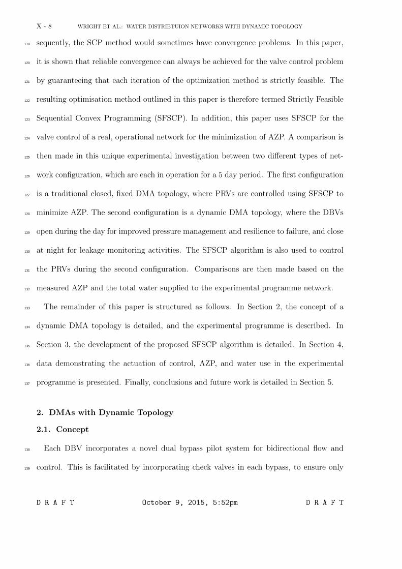
The remainder of this paper is structured as follows. In Section 2, the concept of a133

dynamic DMA topology is detailed, and the experimental programme is described. In134

Section 3, the development of the proposed SFSCP algorithm is detailed. In Section 4,135

data demonstrating the actuation of control, AZP, and water use in the experimental136

programme is presented. Finally, conclusions and future work is detailed in Section 5.137

2. DMAs with Dynamic Topology

2.1. Concept

Each DBV incorporates a novel dual bypass pilot system for bidirectional flow and138

control. This is facilitated by incorporating check valves in each bypass, to ensure only139

D R A F T October 9, 2015, 5:52pm D R A F T

WRIGHT ET AL.: WATER DISTRIBTUION NETWORKS WITH DYNAMIC TOPOLOGY X - 9

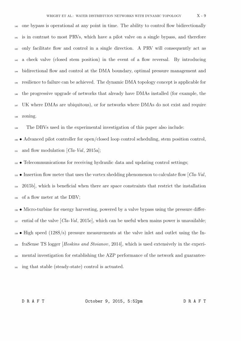
one bypass is operational at any point in time. The ability to control flow bidirectionally140

is in contrast to most PRVs, which have a pilot valve on a single bypass, and therefore141

only facilitate flow and control in a single direction. A PRV will consequently act as142

a check valve (closed stem position) in the event of a flow reversal. By introducing143

bidirectional flow and control at the DMA boundary, optimal pressure management and144

resilience to failure can be achieved. The dynamic DMA topology concept is applicable for145

the progressive upgrade of networks that already have DMAs installed (for example, the146

UK where DMAs are ubiquitous), or for networks where DMAs do not exist and require147

zoning.148

The DBVs used in the experimental investigation of this paper also include:149

Advanced pilot controller for open/closed loop control scheduling, stem position control,150

and flow modulation [Cla-Val , 2015a];151

Telecommunications for receiving hydraulic data and updating control settings;152

Insertion flow meter that uses the vortex shedding phenomenon to calculate flow [Cla-Val ,153

2015b], which is beneficial when there are space constraints that restrict the installation154

of a flow meter at the DBV;155

Micro-turbine for energy harvesting, powered by a valve bypass using the pressure differ-156

ential of the valve [Cla-Val , 2015c], which can be useful when mains power is unavailable;157

High speed (128S/s) pressure measurements at the valve inlet and outlet using the In-158

fraSense TS logger [Hoskins and Stoianov , 2014], which is used extensively in the experi-159

mental investigation for establishing the AZP performance of the network and guarantee-160

ing that stable (steady-state) control is actuated.161

D R A F T October 9, 2015, 5:52pm D R A F T

X - 10 WRIGHT ET AL.: WATER DISTRIBTUION NETWORKS WITH DYNAMIC TOPOLOGY

The DBVs add redundancy to the network and reduce the total frictional head losses162

occurring. By retrofitting PRVs (either existing or newly installed) in the network with163

the same technology, optimal control can be remotely actuated, and the AZP can be164

reduced in a way that takes advantage of the reduced head losses that occur, as discussed165

in Section 1.166

Before DMAs are hydraulically connected using the technology outlined above, it is167

necessary to investigate the potential for negative effects or challenges that might arise as168

a result of dynamic DMA aggregation. First, the mixing of water from different sources,169

with a different water quality, can result in consumers receiving water of different quali-170

ties at different times. This can cause problems for certain industrial users, where their171

processes have been calibrated for a certain type of water quality [World Health Organi-172

zation, 2004]. Any industrial users that could be affected by mixing should be consulted173

before implementing a dynamic DMA topology. In a similar way, residential customers174

could be affected if they perceive the water to change in quality. Hydraulic modelling175

and laboratory testing can also be used to ensure customers are not negatively affected176

by mixing, a process that should be undertaken for any multi-feed WDN [World Health177

Organization, 2004]. Second, contamination can spread further in networks where DMAs178

do not exist, or where DMAs are hydraulically connected using a dynamic topology. It is179

important for a water company to carefully balance this risk with the benefits gained from180

operating a dynamic DMA topology. A valuable step would be collaboration with water181

companies that do not use DMAs on their network to understand mitigation and incident182

management related to contamination. Finally, the dynamic aggregation of DMAs compli-183

cates the valve control of the network for pressure management compared with single-feed184

D R A F T October 9, 2015, 5:52pm D R A F T

WRIGHT ET AL.: WATER DISTRIBTUION NETWORKS WITH DYNAMIC TOPOLOGY X - 11

DMAs. This paper addresses this challenge with the development of the SFSCP algorithm185

presented in Section 3.186

The challenges outlined above should then be compared with the advantages of operat-187

ing a dynamic DMA topology, which can be summarised as follows:188

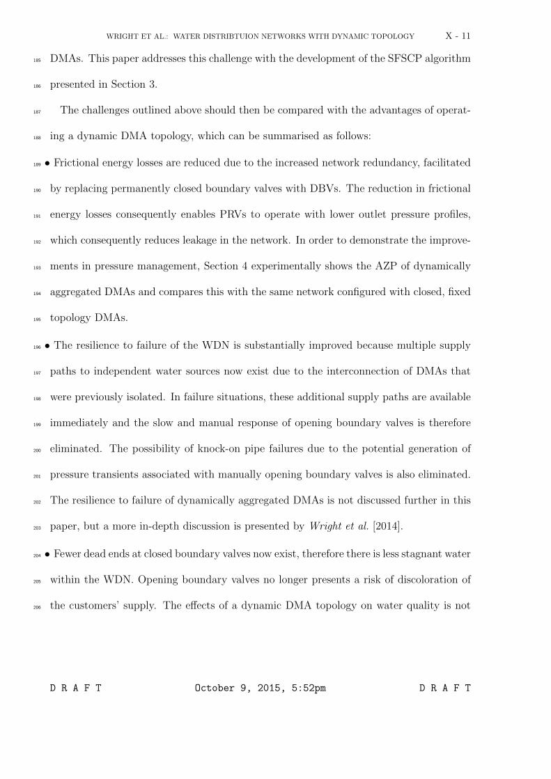
Frictional energy losses are reduced due to the increased network redundancy, facilitated189

by replacing permanently closed boundary valves with DBVs. The reduction in frictional190

energy losses consequently enables PRVs to operate with lower outlet pressure profiles,191

which consequently reduces leakage in the network. In order to demonstrate the improve-192

ments in pressure management, Section 4 experimentally shows the AZP of dynamically193

aggregated DMAs and compares this with the same network configured with closed, fixed194

topology DMAs.195

The resilience to failure of the WDN is substantially improved because multiple supply196

paths to independent water sources now exist due to the interconnection of DMAs that197

were previously isolated. In failure situations, these additional supply paths are available198

immediately and the slow and manual response of opening boundary valves is therefore199

eliminated. The possibility of knock-on pipe failures due to the potential generation of200

pressure transients associated with manually opening boundary valves is also eliminated.201

The resilience to failure of dynamically aggregated DMAs is not discussed further in this202

paper, but a more in-depth discussion is presented by Wright et al. [2014].203

Fewer dead ends at closed boundary valves now exist, therefore there is less stagnant water204

within the WDN. Opening boundary valves no longer presents a risk of discoloration of205

the customers supply. The effects of a dynamic DMA topology on water quality is not206

D R A F T October 9, 2015, 5:52pm D R A F T

X - 12 WRIGHT ET AL.: WATER DISTRIBTUION NETWORKS WITH DYNAMIC TOPOLOGY

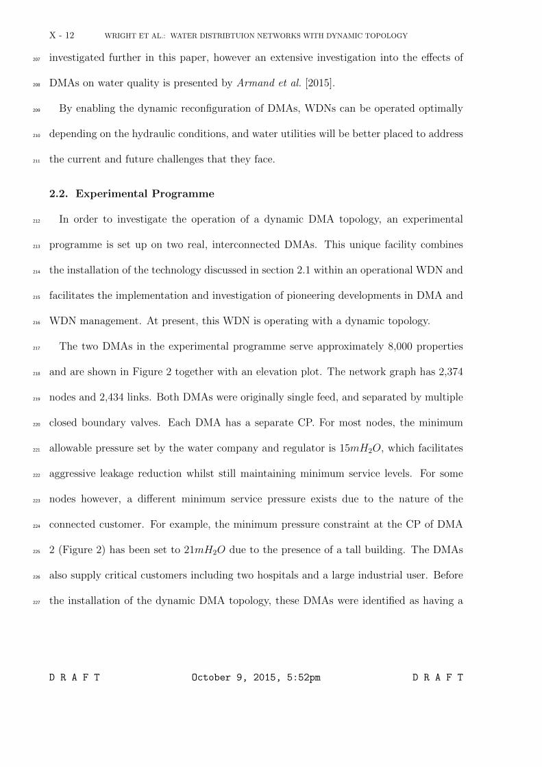
investigated further in this paper, however an extensive investigation into the effects of207

DMAs on water quality is presented by Armand et al. [2015].208

By enabling the dynamic reconfiguration of DMAs, WDNs can be operated optimally209

depending on the hydraulic conditions, and water utilities will be better placed to address210

the current and future challenges that they face.211

2.2. Experimental Programme

In order to investigate the operation of a dynamic DMA topology, an experimental212

programme is set up on two real, interconnected DMAs. This unique facility combines213

the installation of the technology discussed in section 2.1 within an operational WDN and214

facilitates the implementation and investigation of pioneering developments in DMA and215

WDN management. At present, this WDN is operating with a dynamic topology.216

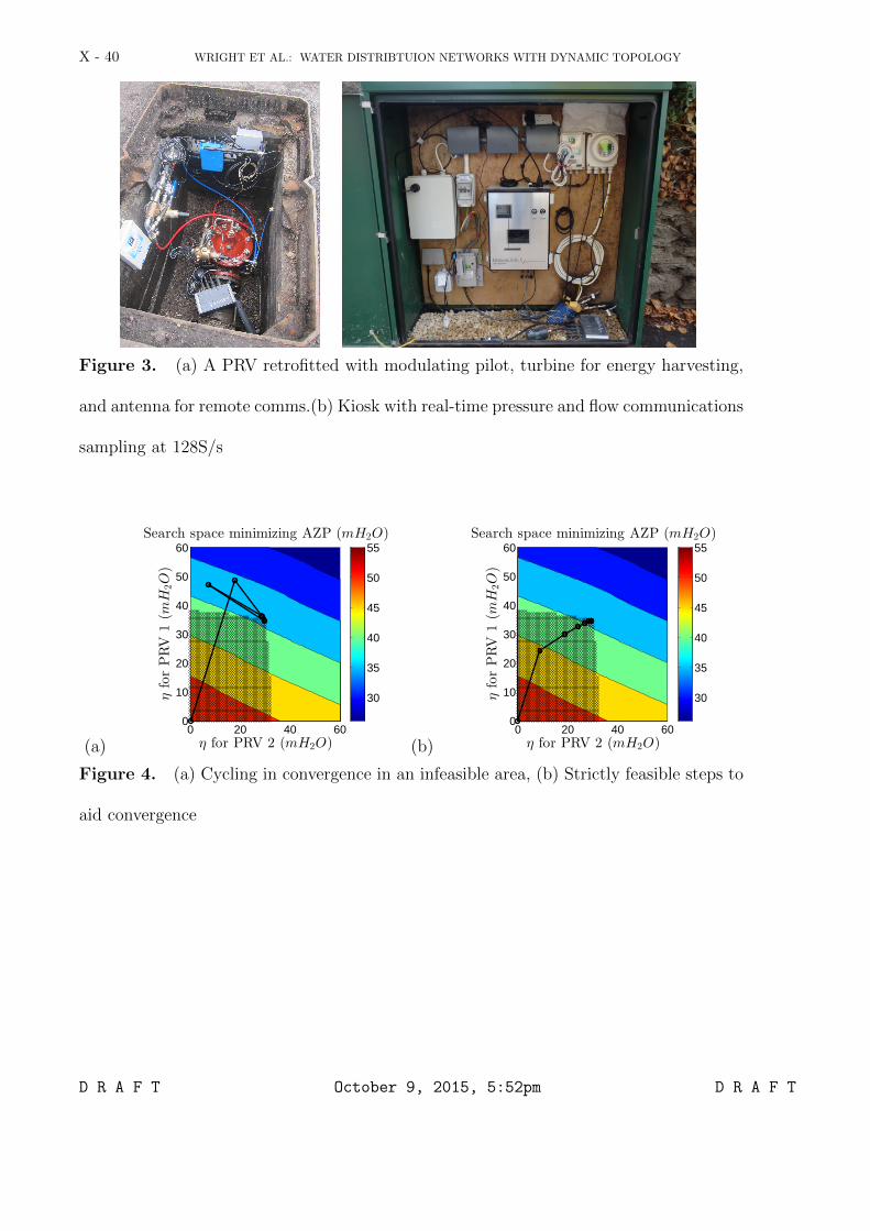
The two DMAs in the experimental programme serve approximately 8,000 properties217

and are shown in Figure 2 together with an elevation plot. The network graph has 2,374218

nodes and 2,434 links. Both DMAs were originally single feed, and separated by multiple219

closed boundary valves. Each DMA has a separate CP. For most nodes, the minimum220

allowable pressure set by the water company and regulator is 15mH2O, which facilitates221

aggressive leakage reduction whilst still maintaining minimum service levels. For some222

nodes however, a different minimum service pressure exists due to the nature of the223

connected customer. For example, the minimum pressure constraint at the CP of DMA224

2 (Figure 2) has been set to 21mH2O due to the presence of a tall building. The DMAs225

also supply critical customers including two hospitals and a large industrial user. Before226

the installation of the dynamic DMA topology, these DMAs were identified as having a227

D R A F T October 9, 2015, 5:52pm D R A F T

WRIGHT ET AL.: WATER DISTRIBTUION NETWORKS WITH DYNAMIC TOPOLOGY X - 13

high AZP and little security of supply for the critical users (hospitals) because only one228

supply route is available for each of the single-feed DMAs.229

The installation of the dynamic DMA topology included the replacement of two closed230

boundary valves with dynamic boundary valves (DBV 1 and DBV 2, as shown in Figure 2),231

and the retrofitting of two PRVs (PRV 1 and PRV 2) with the same technology, which was232

outlined in Section 2.1. An additional 21 sensors that measure pressure at a frequency of233

128S/s (InfraSense TS) are placed throughout the WDN to provide key measurements that234

aid in the calculation of AZP as well as additional information about the control efficiency235

and other events. At control valve sites where power is available, data is communicated236

in real-time via an ADSL link installed in a nearby kiosk as shown in Figure 3 and offers237

instantaneous visibility of the network status. Flow measurements are also transmitted in238

real-time and are used to assess the network behaviour and update demand usage patterns239

in the hydraulic model.240

In this paper, the AZP of two configurations of DMA operation are investigated through241

the experimental programme: a static DMA topology (closed boundary valves) and a242

dynamic DMA topology where the DBVs are programmed to open during the day, and243

close at night for leakage detection activities. The calculation and actuation of optimal244

valve settings for PRV 1 and PRV 2 (Figure 2) in both configurations is undertaken using245

a novel optimization method based on strictly feasible sequential convex programming, as246

outlined in the following section.247

3. Control Optimization

To determine optimal PRV settings in the experimental programme, a mathematical248

optimization problem (that employs the steady-state hydraulic system behavior as a set of249

D R A F T October 9, 2015, 5:52pm D R A F T

X - 14 WRIGHT ET AL.: WATER DISTRIBTUION NETWORKS WITH DYNAMIC TOPOLOGY

nonlinear constraints) is solved. A number of optimization methods have been proposed250

for this purpose and are summarized in Section 3.2. The optimization problem is solved251

multiple times to reflect hydraulic changes (i.e. customer demands, reservoir levels) in252

the WDN. Open-loop PRV settings can therefore be constructed. The implementation of253

these open-loop PRV settings is discussed in section 4.1.254

3.1. Problem Formulation

We consider a demand-driven model for a WDN, which is represented by a graph con-

sisting a set of nodes Nn, where |Nn| = nn, a set of reservoirs No, where |No| = no, a

set of links Np, where |Np| = np, and a set of PRVs Nv, where |Nv| = nv and Nv Np.

The mass and energy conservation laws that describe the WDN are defined by the set of

equations:

g1(q, h, ;h0) := A11(q)q + A12h+ A10h0 + A13 = 0, (1)

g2(q; d) := AT12q d = 0, (2)

where h Rnn are the nodal piezometric heads, q Rnp are the pipe flows, Rnv

are the PRV settings, the matrices A12 Rnpnn , A13 Rnpnv , and A10 Rnpno

are incidence matrices describing the relationship between links and nodes, valves and

reservoirs respectively. The variable d Rnn represents water demand at nodes (assumed

known), h0 Rno are known heads. The square matrix A11 Rnpnp is a diagonal matrix

with the elements

A11(i, i) = ri|qi|ni1, i = 1, . . . , np, (3)

where r Rnp is the vector of frictional resistance factors of the pipes and n Rnp are255

constants related to the frictional head loss. In this article, the Hazen-Williams friction256

D R A F T October 9, 2015, 5:52pm D R A F T

WRIGHT ET AL.: WATER DISTRIBTUION NETWORKS WITH DYNAMIC TOPOLOGY X - 15

formula is used to model frictional losses; ni = 1.85 and ri =10.675Licnii D

4.87i

, where Li, Di and ci257

denote the length, diameter and roughness coefficient of pipe i, respectively. For valves,258

ni = 2 and an empirical value for ri is generally supplied by the valve manufacturer.259

To find the optimal PRV settings that minimize the AZP of the WDN, we solve the

optimization problem:

min,q,h

f(h; , q) :=nnj=1

jhj, (4a)

subject to: g1() = 0 (4b)

g2() = 0 (4c)

qi 0, i Nv (4d)

i 0, i Nv (4e)

hj hj 0, j Nn (4f)

where g1() and g2() are the conservation equations (1) and (2), respectively, and the

inequality constraints (4f) come from the need to satisfy the minimum service level guar-

antees. The component-wise positive constants in h Rnn are the minimum service level

heads for each node. The inequality constraints (4d) and (4e) come from the physical

constraint that PRVs regulate pressure in a single direction. The coefficients Rnn

in (4a) relate the AZP to the nodal pressures by weighting each node by the length of its

incident links. That is,

j = L1

iIj

Li2, L =

npi=1

Li, (5)

where Ij is the set of indices for links incident at node j and Li is the length of the ith260

pipe.261

D R A F T October 9, 2015, 5:52pm D R A F T

X - 16 WRIGHT ET AL.: WATER DISTRIBTUION NETWORKS WITH DYNAMIC TOPOLOGY

In the optimization problem (4), PRVs are modelled using the linear term , which262

represents the additional head loss within links containing a PRV. Therefore, if for PRV263

i, i = 0, the PRV is fully open, and the total head differential is equal a minor loss repre-264

sented by riqnii for the valve. Although (4) has a linear objective (4a) and linear inequality265

constraints(4d)(4f), the equality constraint for energy conservation (4b) is nonlinear due266

to the nonlinear frictional loss terms of the form riqi|qi|ni1. This results in a nonlinear267

program (NLP) that is also non-convex, since flow in pipes is bi-directional. In addition,268

the use of the Hazen-Williams head loss formula means the problem is non smooth at flows269

qi = 0. Although generic NLP solvers can be used to solve (4), greater computational270

efficiency and reliability of solutions can be achieved if the problem structure is taken into271

account [Wright et al., 2014]. This is particularly important when implementing real-time272

control and so is our approach in this article.273

3.2. Review of valve optimization

Optimization of valve control has generally been studied with the intention of reduc-274

ing either pressure or leakage in WDNs. Jowitt and Xu [1990] used a sequential linear275

programming (SLP) method to minimize leakage for a small example network consisting276

of 25 nodes. Vairavamoorthy and Lumbers [1998] used the same network to demonstrate277

a sequential quadratic programming (SQP) method. In addition, an objective function278

that minimizes the difference between target and actual nodal pressure was investigated,279

which allows minor pressure violations at nodes in order to achieve a larger overall re-280

duction in network pressure. Ulanicki et al. [2000] solved an NLP for reducing leakage in281

simulation by using a commercial NLP solver. In addition, each optimized valve profile282

was correlated with the valves flow to produce a control curve (also called a flow modu-283

D R A F T October 9, 2015, 5:52pm D R A F T

WRIGHT ET AL.: WATER DISTRIBTUION NETWORKS WITH DYNAMIC TOPOLOGY X - 17

lation curve), an approach that is used in this paper to actuate control (Section 4.1). For284

large networks, Ulanicki et al. [2000] used the model skeletonization technique proposed285

by Ulanicki et al. [1996] to reduce the computation time. Skworcow et al. [2010] used the286

same NLP solver for the combined optimization of PRVs and pumps on a skeletonized287

network. They proposed model predictive control (MPC) for the control implementation.288

MPC involves the periodic finite-time optimization of the future state of the WDN model289

and the calculation and implementation of optimal valve settings based on this future290

horizon. Due to limitations in telecommunications, the MPC approach was only used in291

simulation.292

The simultaneous optimization of valve placement and valve settings was considered in293

(Eck and Mevissen [2013], Eck and Mevissen [2012]). A key aspect of their implemen-294

tation was the approximation of the Hazen-Williams relationship by quadratic function.295

Two variables representing flows in opposite directions were assigned to each pipe but296

with a complementarity condition that at least one of the flows is zero. This approach297

therefore avoids the discontinuity at qi = 0 when using the Hazen-Williams head loss298

formula. Two case studies were used: the small illustrative network from Jowitt and Xu299

[1990] and a larger network (Exnet) consisting of approximately 1,900 nodes introduced300

to the research community as a more realistic WDN model by Farmani et al. [2004]. The301

quadratic approximation resulted in a pressure and flow solution that generally agreed well302

with hydraulic simulation solutions from EPANET although some reported errors were as303

high as 0.75l/s. The recorded solution time for optimizing the settings of 4 control valves304

(fixed valve placements) in Exnet was 121 seconds. Nicolini and Zovatto [2009] also305

solved a combined valve placement and control problem using genetic algorithms (GA),306

D R A F T October 9, 2015, 5:52pm D R A F T

X - 18 WRIGHT ET AL.: WATER DISTRIBTUION NETWORKS WITH DYNAMIC TOPOLOGY

which are particularly useful when multiple objective functions are evaluated. Whilst307

heuristics such as GA are highly applicable to design problems and often find good solu-308

tions in the search space, they generally require high computation times due to the large309

number of hydraulic simulations involved in finding a good solution and are not generally310

appropriate for near real-time control applications.311

For the optimization method used for PRV control in our experimental programme, a312

number of strict criteria were set out that have not all been addressed by previous work313

in the literature. The criteria are as follows:314

Reliable convergence: An optimization method used in near real-time control must be315

able to perform under a wide range of hydraulic conditions and produce a control solution316

consistently.317

Rapid convergence: The optimization should also be computationally cheap to carry out.318

This ensures that valve settings can be calculated rapidly when hydraulic changes occur319

in the network. It also facilitates the optimization to be run on less powerful computers320

or servers, making it accessible to more users.321

An exact representation of the hydraulic model without simplification or skeletonization.322

This ensures as much accuracy is retained as possible in the control solution and also323

aids in the scalability of the solution method to bigger networks or different objective324

functions.325

An optimization method based on SCP was proposed in [Wright et al., 2014] that326

addressed the above criteria. An SCP method solves a non-convex NLP problem by se-327

quentially solving convex approximations (sub-problems). The convexity of each approx-328

imation means each sub-problem can be solved accurately and efficiently. SCP methods329

D R A F T October 9, 2015, 5:52pm D R A F T

WRIGHT ET AL.: WATER DISTRIBTUION NETWORKS WITH DYNAMIC TOPOLOGY X - 19

differ from other sequential optimisation methods (SLP, SQP) because they preserve con-330

vexity in the problem, even if this convexity is non-linear [Dinh et al., 2011]. SCP was331

used by [Quoc et al., 2012] to successfully solve near real-time control problems. Its ma-332

jor advantage is that it can generally converges well to a feasible point with a good or333

optimal objective function value. In [Wright et al., 2014], the SCP method was applied to334

a PRV control problem and showed good convergence properties under various different335

hydraulic conditions. In this paper, we are interested in controlling PRVs and DBVs.336

The introduction of DBVs that follows a position controlled schedule (i.e. open in the337

day, closed at night) resulted in the SCP method from [Wright et al., 2014] occasionally338

getting stuck outside the feasible optimization search space. In this paper, we improve339

the convergence of the SCP method by guaranteeing that each step in the optimization340

is strictly feasible.341

3.3. Strictly Feasible Sequential Convex Programming for Valve Optimization

Let the optimization variables and the equality constraints of (4b)(4c) be reformulated

as x := [qT hT T ]T and g(x) := [g1(x)T g2(x)

T ]T Rnp+nn , respectively. We define the

hydraulic feasibility region by the set

E := {x Rnp+nn+nv : x satisfies (4b), (4c), (4d), and (4e)}. (6)

Similarly, the inequality feasibility region for the PRV setting and performance con-

straints is defined by the set

F := {x Rnp+nn+nv : x satisfies (4d), (4e) and (4f)}. (7)

When the SCP framework [Quoc et al., 2012] is applied to (4) for given parameters d342

and h0, the algorithm structure is as follows:343

D R A F T October 9, 2015, 5:52pm D R A F T

X - 20 WRIGHT ET AL.: WATER DISTRIBTUION NETWORKS WITH DYNAMIC TOPOLOGY

Step 1. Choose a hydraulically feasible x1 E, Set k = 1344

Step 2. To get the new iterate xk+1, solve the convex subproblem:

minx

cTx (8a)

subject to:

g(xk)(x xk) + g(xk) = 0, (8b)

x F (8c)

where the coefficient vector c contains the vector of weights wi and g(x) is the Jaco-345

bian of the constraint matrix g.346

Step 3. STOP IF stopping criteria is satisfied. ELSE, set k to k + 1 and Go back to Step 2.347

The subproblem (8) is formed by linearizing the equality constraints, specifically (4b).

The equality constraint (8b) has the expression

NA11(qk)(q qk) + A11(qk)qk + A12h+

A10h0 + A13 = 0, (9a)

AT12q d = 0, (9b)

in terms of the flows, heads and PRV settings, where N = diag(ni), i = 1, . . . , np. With348

xk being a known constant at the current iteration k, the constraints (9) are all linear in349

the unknown x. Therefore, the resulting optimization problem (8) has a linear objective350

and linear equality and inequality constraints; it is, therefore, a convex program and can351

be solved efficiently [Luenberger and Ye, 2008]. This makes the SCP approach even more352

attractive since state-of-the art interior-point solvers can be used even for large scale linear353

programs, where the sparsity structures in the constraints are taken advantage of Nocedal354

and Wright [2006].355

D R A F T October 9, 2015, 5:52pm D R A F T

WRIGHT ET AL.: WATER DISTRIBTUION NETWORKS WITH DYNAMIC TOPOLOGY X - 21

In [Wright et al., 2014], this SCP framework was investigated. Although the iterates356

xk+1 that solve (8) satisfy the linear equality constraint(4c), they would not satisfy the357

nonlinear equality (4b) and so would not be hydraulically feasible. In principle, these358

iterates can be projected onto the intersection of hydraulic feasibility and performance359

inequality constraint sets EF. Even for convex nonlinear constraint sets, the substantial360

overhead associated with projected methods is a main drawback [Bertsekas , 1999, Sec.361

2.3]. Since the effort of projecting the solution xk+1 F onto the intersection of the linear362

and nonlinear constraint sets can be as complicated as solving the original optimization363

problem, an approximate approach to projection was used in [Wright et al., 2014] to364

maintain hydraulic feasibility at each step.365

The method starts by solving a hydraulic equation, where the PRVs are set to fully366

open for the first iteration. With the PRV setting 1 = 0, (1) and (2) are solved to find367

q1 and h1 such that x1 E. After Step 2 of each iteration k, the value k+1 from the368

solution xk+1 F of (8) was fixed as the PRV setting and a hydraulic solver was used369

to find another qk+1 and hk+1 that satisfy (1) and (2) for this PRV setting; i.e. a sort of370

projection of xk+1 onto the hydraulic feasibility set E is used to guarantee the hydraulic371

conservation equations are satisfied. A sort of projection because the updated values372

qk+1 and hk+1 may not satisfy the performance constraints, i.e. xk+1 = [qk+1; hk+1; k+1]373

may not be in F. Setting k to k + 1, the linearized convex problem in Step 2 was then374

solved with xk+1. This process was repeated until the objective function evaluated for375

xk E decreased sufficiently and the difference between the linear program solution and376

its projection onto the hydraulic feasibility set E, i.e. xk+1xk+1, was within a specified377

small tolerance.378

D R A F T October 9, 2015, 5:52pm D R A F T

X - 22 WRIGHT ET AL.: WATER DISTRIBTUION NETWORKS WITH DYNAMIC TOPOLOGY

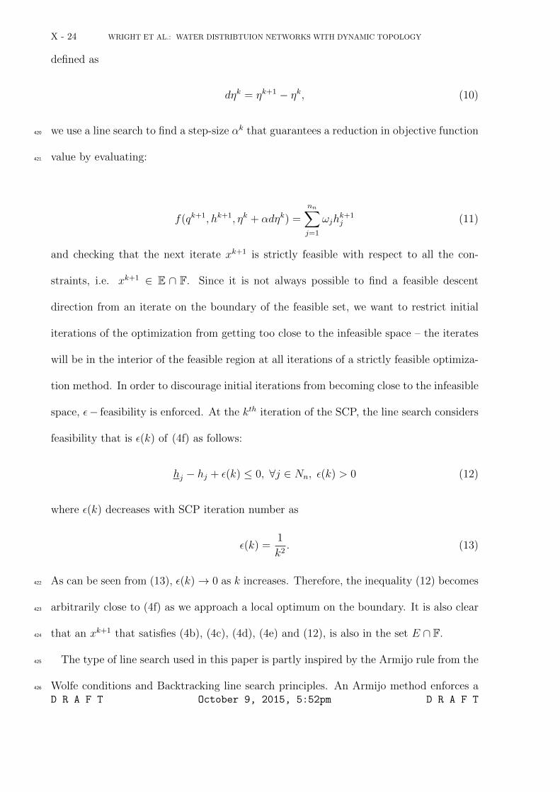
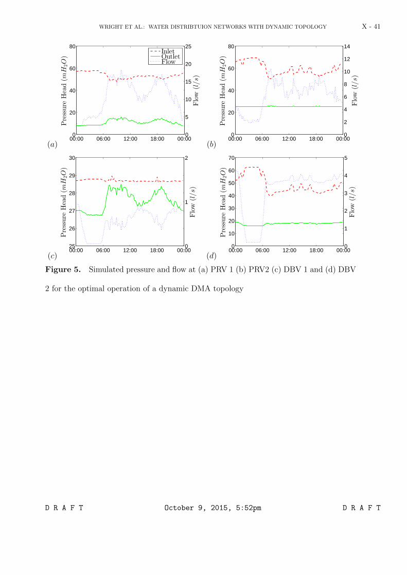
It was shown in [Wright et al., 2014] that this approach worked well most of the time.379

However, the method sometimes failed to converge to a feasible solution for the original380

optimization problem (4). For example, k+1 computed at Step 2 would sometimes result381

in a solution that violates (4f) when projected onto E, which occasionally led to conver-382

gence difficulties. One example of this is shown in Figure 4a. Here, the SCP method from383

[Wright et al., 2014] is applied to the case study in Figure 2. The contours represent the384

objective function when two PRVs are operational and the shaded region represents the385

feasible region EF, i.e. the space where the constraints (4b) (4f) are all satisfied. The386

optimization method takes steps outside of the feasibility region initially, and eventually387

oscillates in an infeasible search space for the original optimization problem (4). This388

either resulted in an infeasible solution after the maximum number of iterations or in389

sub-optimality when the final solution was projected onto the feasibility region.390

In this article, we propose the use of strictly feasible iterates to stabilize the algorithm391

and to achieve convergence. In the spirit of feasible direction descent methods [Bertsekas ,392

1999, Sec 2.2], we generate a sequence of feasible iterates by using line searches along393

descent directions; in our strictly feasible SCP, a simple line search is used to guarantee a394

descent in the objective function and feasibility at each iteration, which together guarantee395

convergence to a local minima. The SFSCP algorithm can only guarantee convergence396

to locally optimal solutions because the original problem is nonconvex. Although it is397

generally not possible to show a linear or better rate of convergence for SCP methods, we398

do not attempt to prove convergence properties as it is beyond the scope of this paper.399

SCP methods can also sometimes have slow convergence very near to solutions [Schit-400

tkowski and Zillober , 2005]. Nonetheless, SCP methods are generally known to have fast401

D R A F T October 9, 2015, 5:52pm D R A F T

WRIGHT ET AL.: WATER DISTRIBTUION NETWORKS WITH DYNAMIC TOPOLOGY X - 23

convergence to optimal points in many practical optimization problems [Ni et al., 2005].402

As will be shown in Section 4.1, this is the case in our optimization problem.403

For a given feasible iterate xk, a feasible direction at xk is a non-zero vector dk that404

guarantees xk +dk is feasible for all (0, ] with some > 0 that is sufficiently small.405

From Figure 4a, we note that the first iterate of the SCP is taken along a feasible descent406

direction. Since the descent direction is one that reduces pressure heads, taking a full-407

step in this direction can violate the minimum pressure constraints (4f). Moreover, if the408

feasible iterate is on the boundary of the feasibility space EF, where the constraints (4f)409

are active, the descent directions may not even be feasible. Like feasible interior point410

methods [Nocedal and Wright , 2006], we propose making our iterates strictly feasible by411

approaching the boundary of EF from the interior of the constraints (4f). Unlike interior412

point methods we do not use barrier function but rather enforce strict feasibility in the413

projection stage of our SCP approach.414

In this new approach, the valve settings k+1, which are computed by solving the linear415

program in Step 2 of the kth iteration in SCP algorithm, are not used directly to find416

a projection/solution in E via hydraulic simulations. Instead, k+1 is used to form a417

feasible descent direction, and a line search is performed to find a next iteration that is418

guaranteed to be both feasible and lower in objective function value.419

3.4. Line Search

Line search methods are used in optimization to determine step sizes that minimize or

decrease the objective function f() along a search direction. With the search direction

D R A F T October 9, 2015, 5:52pm D R A F T

X - 24 WRIGHT ET AL.: WATER DISTRIBTUION NETWORKS WITH DYNAMIC TOPOLOGY

defined as

dk = k+1 k, (10)

we use a line search to find a step-size k that guarantees a reduction in objective function420

value by evaluating:421

f(qk+1, hk+1, k + dk) =nnj=1

jhk+1j (11)

and checking that the next iterate xk+1 is strictly feasible with respect to all the con-

straints, i.e. xk+1 E F. Since it is not always possible to find a feasible descent

direction from an iterate on the boundary of the feasible set, we want to restrict initial

iterations of the optimization from getting too close to the infeasible space the iterates

will be in the interior of the feasible region at all iterations of a strictly feasible optimiza-

tion method. In order to discourage initial iterations from becoming close to the infeasible

space, feasibility is enforced. At the kth iteration of the SCP, the line search considers

feasibility that is (k) of (4f) as follows:

hj hj + (k) 0, j Nn, (k) > 0 (12)

where (k) decreases with SCP iteration number as

(k) =1

k2. (13)

As can be seen from (13), (k) 0 as k increases. Therefore, the inequality (12) becomes422

arbitrarily close to (4f) as we approach a local optimum on the boundary. It is also clear423

that an xk+1 that satisfies (4b), (4c), (4d), (4e) and (12), is also in the set E F.424

The type of line search used in this paper is partly inspired by the Armijo rule from the425

Wolfe conditions and Backtracking line search principles. An Armijo method enforces a426D R A F T October 9, 2015, 5:52pm D R A F T

WRIGHT ET AL.: WATER DISTRIBTUION NETWORKS WITH DYNAMIC TOPOLOGY X - 25

sufficient decrease in the objective along the descent direction [Bertsekas , 1999]. Since a427

full step will not necessarily maintain strict feasibility of all constraints, we instead only428

require that f() decreases at each iteration. For practical purposes this works well, since429

f() decreases rapidly along the search directions dk as seen in Figure 4b, and quickly430

gets very close to a local minimum.431

In Backtracking line searches, initially the full step is taken (i.e. = 1) and subse-432

quently reduced until a stopping condition is satisfied [Boyd and Vandenberghe, 2004].433

The same principle is used in this paper by first taking a unit step ( = 1) and updating434

subsequently until the line search stopping criteria are satisfied. The stopping criteria435

is that the next iterate is feasible (EF) and that it has a lower objective function value.436

The line search is carried out using a two step process as follows. For the first iteration437

of the line search, = 1 and438

1. Compute f(, k + dk+1)439

2. IF f(, k +dk) < f(, k) AND the next iterate is feasible, then k+1 = k +dk440

ELSE set = /2, return to return to step 1441

For the example shown in Figure 4a, this process of ensuring iterations are strictly442

feasible is shown in Figure 4b. Here it is guaranteed that each step both decreases f()443

and is strictly inside the feasible set EF shown by the shaded area. In the latter iterations444

of the optimization, allowing the k to become sufficiently small enables the solutions to445

get arbitrarily close to the local optima. Moreover, a practical stopping criteria that the446

relative decrease in the objective function is within some tolerance tol is used here, i.e.447

termination is triggered when fkfk+1fk

< tol. In our examples, we found that a value of448

D R A F T October 9, 2015, 5:52pm D R A F T

X - 26 WRIGHT ET AL.: WATER DISTRIBTUION NETWORKS WITH DYNAMIC TOPOLOGY

103 for tol was sufficiently small. Our SFSCP method is summarised in Algorithm 1,449

where we denote a hydraulic simulation that solves (1) and (2) by HS.450

3.5. Hydraulic analysis for equality constraints

In [Wright et al., 2014], (1) and (2) was solved only once at each iteration of the opti-451

mization method. The solution was calculated using a Newton method initially proposed452

by Todini and Pilati [1988] and commonly referred to as the nodal Newton-Raphson453

method. In this paper, the solution to (1) and (2) is calculated at least twice for each454

iteration of the optimization method. When calculating PRV settings for extended period455

simulations, this can lead to a large increase in computing time. The solution to (1) and456

(2) represents the most computationally intensive part of our optimization method. We457

therefore require an efficient method for the hydraulic analysis problem. In [Abraham and458

Stoianov , 2015], a null space algorithm for hydraulic analysis is shown to have superior459

computational efficiency for hydraulic analysis of sparse networks. The structure of the460

system of equations in (1) and (2) is that of a saddle point system, which null space461

algorithms take advantage of. The method starts with an initial solution to (2) by using,462

for example, a least square method. A null space basis is then generated and further463

Newton iterations are carried out in this space until (1) is also satisfied. The method464

offers strong improvements in computational speed particularly when np nn is small,465

which is generally the case for most real networks [Elhay et al., 2014]. In [Abraham and466

Stoianov , 2015], further computational efficiency is achieved by carrying out updates of467

headlosses at each Newton iteration only for links whose flows have not yet converged.468

Another advantage of using the null space algorithm is its ability to handle links with469

a zero flow. Typically, methods such as the nodal Newton scheme do not accurately470

D R A F T October 9, 2015, 5:52pm D R A F T

WRIGHT ET AL.: WATER DISTRIBTUION NETWORKS WITH DYNAMIC TOPOLOGY X - 27

calculate zero flows, which can result in poor convergence when used in optimization471

problems. This is because when qi = 0, A111 (q) becomes singular when using the Hazen-472

Williams head loss formula. The optimization of WDNs with a dynamic topology will473

always have zero flows because the boundary valves generally close at night resulting in474

a zero flow between interconnected DMAs. In the null space approach, no such matrix475

inversion is required. Moreover, by using a Jacobian regularization within the null space476

algorithm, it is possible to avoid ill-conditioning of the linear systems of the Newton477

method.478

479

Data: Network structure, configuration and hydraulic data (A12, A10, A13, H0, d)Result: Valve settings ()Initialization: Set = 0, k = 1;

hk, qk HS(k);while fk fk+1 > tol and k kmax do

k+1 solution to (8) ;dk k+1 k ;Set = 1;

hk+1, qk+1 HS(k + dk);while fk+1 > fk or xk+1 / E F do

/2;hk+1, qk+1 HS(k + dk);

end

k+1 k + dk;k k + 1

endAlgorithm 1: SFSCP

480

D R A F T October 9, 2015, 5:52pm D R A F T

X - 28 WRIGHT ET AL.: WATER DISTRIBTUION NETWORKS WITH DYNAMIC TOPOLOGY

4. Results and Discussion

4.1. Optimization Results

The SFSCP algorithm outlined in the previous section was used to calculate open-loop481

pressure profiles for PRV 1 and PRV 2 in the experimental programme shown in Figure 2482

for both a closed DMA topology and a dynamic DMA topology. In all simulations, SFSCP483

successfully converged to a local optimal control solution, with an average of 9 iterations484

required to meet the convergence criterion.485

This section only details the implementation of the optimized PRV settings in the486

dynamic DMA topology configuration. The implementation of the PRV settings for the487

closed DMA configuration follows the same procedure, with the exception that the bound-488

ary valves are fully closed at all times. The comparison of AZP are then shown for both489

a dynamic and closed DMA topology.490

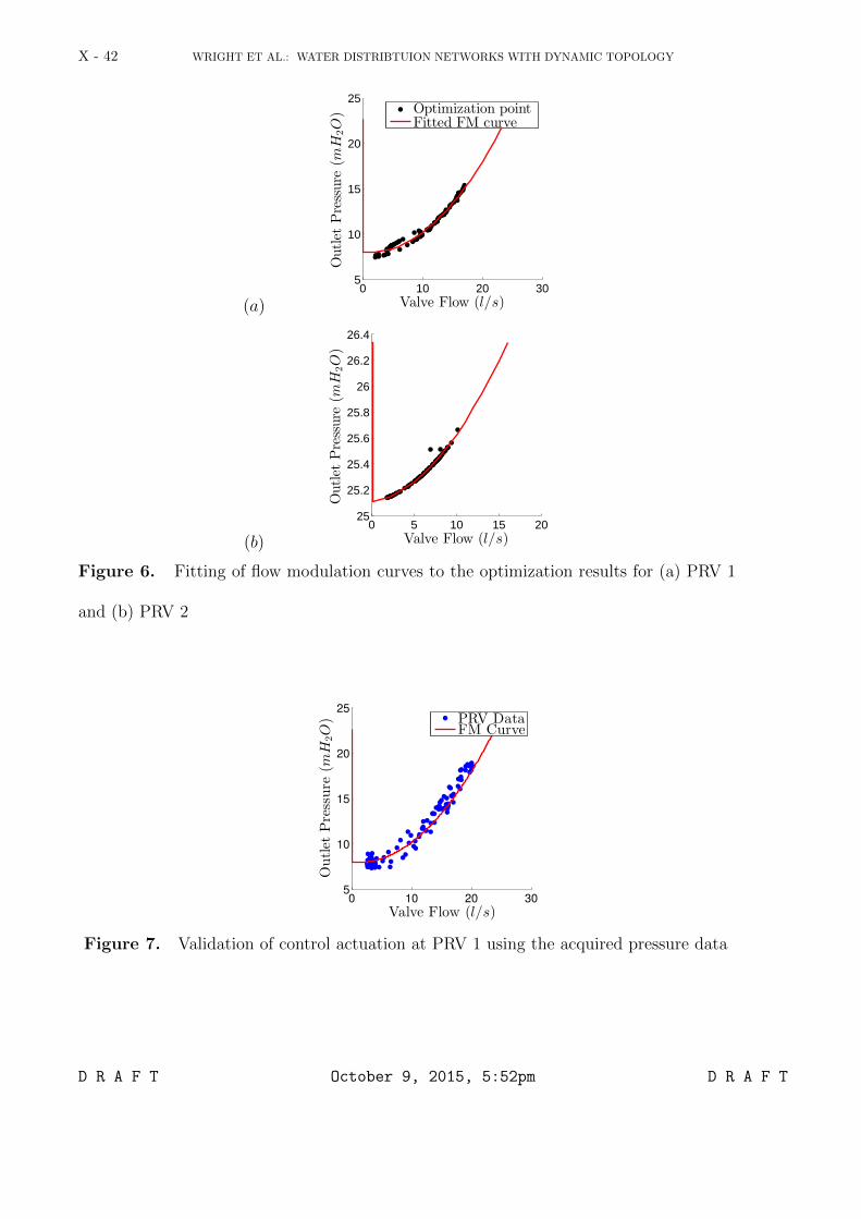
The optimized PRV outlet pressure profiles are shown in Figure 5a and Figure 5b. It491

is observed that each PRV outlet pressure is correlative to the PRV flow, therefore it is492

possible to establish and implement a flow modulation curve, i.e. a relationship between493

outlet pressure and flow. This facilitates near optimal valve settings to be actuated locally494

on each PRV using local flow measurements captured with a flow meter. Flow modulation495

is an emerging form of advanced pressure management. There are many suppliers of the496

technology [Technolog , 2014; i2O , 2014; Palmer , 2015] and consequently flow modulation497

is becoming increasingly implemented in industry. More information on flow modulation498

and other PRV control approaches is reviewed by Ulanicki et al. [2000] and Wright et al.499

[2014].500

D R A F T October 9, 2015, 5:52pm D R A F T

WRIGHT ET AL.: WATER DISTRIBTUION NETWORKS WITH DYNAMIC TOPOLOGY X - 29

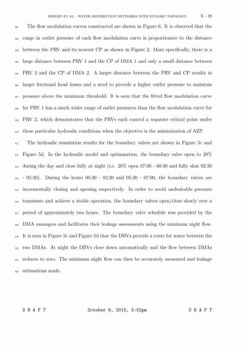
The flow modulation curves constructed are shown in Figure 6. It is observed that the501

range in outlet pressure of each flow modulation curve is proportionate to the distance502

between the PRV and its nearest CP as shown in Figure 2. More specifically, there is a503

large distance between PRV 1 and the CP of DMA 1 and only a small distance between504

PRV 2 and the CP of DMA 2. A larger distance between the PRV and CP results in505

larger frictional head losses and a need to provide a higher outlet pressure to maintain506

pressure above the minimum threshold. It is seen that the fitted flow modulation curve507

for PRV 1 has a much wider range of outlet pressures than the flow modulation curve for508

PRV 2, which demonstrates that the PRVs each control a separate critical point under509

these particular hydraulic conditions when the objective is the minimization of AZP.510

The hydraulic simulation results for the boundary valves are shown in Figure 5c and511

Figure 5d. In the hydraulic model and optimization, the boundary valve open to 20%512

during the day and close fully at night (i.e. 20% open 07:00 - 00:30 and fully shut 02:30513

- 05:30). During the hours 00:30 - 02:30 and 05:30 - 07:00, the boundary valves are514

incrementally closing and opening respectively. In order to avoid undesirable pressure515

transients and achieve a stable operation, the boundary valves open/close slowly over a516

period of approximately two hours. The boundary valve schedule was provided by the517

DMA managers and facilitates their leakage assessments using the minimum night flow.518

It is seen in Figure 5c and Figure 5d that the DBVs provide a route for water between the519

two DMAs. At night the DBVs close down automatically and the flow between DMAs520

reduces to zero. The minimum night flow can then be accurately measured and leakage521

estimations made.522

D R A F T October 9, 2015, 5:52pm D R A F T

X - 30 WRIGHT ET AL.: WATER DISTRIBTUION NETWORKS WITH DYNAMIC TOPOLOGY

4.2. Experimental Programme Implementation

PRV 1 and PRV 2 are uploaded with the flow modulation curves shown in Figure 6 and523

the DBVs follow the opening schedule defined in section 4.1. The experimental programme524

network is monitored using the real time data and analyzed for the following:525

Actuation of control: It is important to ensure that the optimized valve settings have526

been actuated correctly at the PRVs. This is undertaken by analyzing the data at the527

PRVs and comparing this with the flow modulation curve. For example, Figure 7 shows528

the hydraulic data for PRV 1 and the flow modulation curve derived from the optimization529

that it follows. The PRV successfully follows the curve with an R2 value of 0.94.530

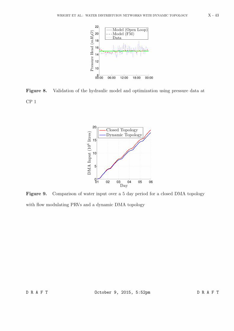
Model and data comparison: This involves the comparison of the model pressure at nodes531

where data is available. For example, Figure 8 shows the pressure at CP 1 (Figure 2)532

according to the hydraulic model (simulated with both the optimal open-loop PRV settings533

and the fitted flow modulation curves defined in Figure 6 for PRV 1 and PRV 2), and534

pressure data from a remote logger deployed at CP 1 (data plotted at 5 samples/s).535

The pressure at CP 1 according to the hydraulic model when optimal open-loop valve536

settings are used at the PRVs is exactly 15mH2O, which represents the minimum allowable537

pressure. This is to be expected, since the objective function was to minimize AZP subject538

to a minimum allowable pressure. By using the optimal outlet pressure profiles in the539

hydraulic model, this target pressure is achieved at the CP. When the flow modulation540

curves are used for PRV 1 and PRV 2 in the hydraulic model, pressure at CP 1 remains541

close to 15mH2O but fluctuates above and below this value. This is because there are542

some small discrepancies between the flow modulation curve and the optimal valve set543

point (Figure 6). Finally, the hydraulic data also shows that pressure at the CP is also544

D R A F T October 9, 2015, 5:52pm D R A F T

WRIGHT ET AL.: WATER DISTRIBTUION NETWORKS WITH DYNAMIC TOPOLOGY X - 31

fluctuating above and below CP 1. A minimum pressure value of 13.27mH2O occurs.545

Discrepancies here are due to the stochastic nature of customer demand, uncertainty in546

the hydraulic model, and the discrepancies between the optimal PRV set point and the547

flow modulation curve. The data shows that the PRV control has successfully controlled548

pressure such that the CP is close to 15mH2O. This methodology for checking the valve549

actuation and network behaviour is repeated for other points of the WDN to further550

validate the optimization method, hydraulic model and control. As recommended by551

[Committee et al., 1999], pressure measurements are within 2mH2O of the steady state552

hydraulic model for 100% of the logged nodes.553

In order to assess the AZP benefits of operating a dynamic DMA topology over a closed,554

static DMA topology, the experimental programme is operated consequently using the555

two configurations outlined above, each for a 5 day period. The first configuration has a556

dynamic topology (where BV1 and BV2 open to 20% each day) and the flow modulation557

curves shown in Figure 6 controlling PRV 1 and PRV 2. The second configuration has a558

closed DMA topology (i.e. BV1 and BV2 set to 100% closed at all times) and optimized559

flow modulation curves configured on the PRV 1 and PRV 2 that were calculated using560

the SFSCP methodology. The total WDN water input is then measured using the flow561

meters and the results are shown in Figure 9. It is observed that over the 5 day period,562

approximately 1 million less litres are used in the DMAs of the experimental programme563

when a dynamic topology is in operation, which is a reduction of approximately 5%. A564

reduction in AZP of 2.8% was also observed using the hydraulic model. Although the565

length of this case study is limited, it shows that a dynamic topology provides promising566

results for the reduction of AZP and leakage. Based on the modelling and the SFSCP567

D R A F T October 9, 2015, 5:52pm D R A F T

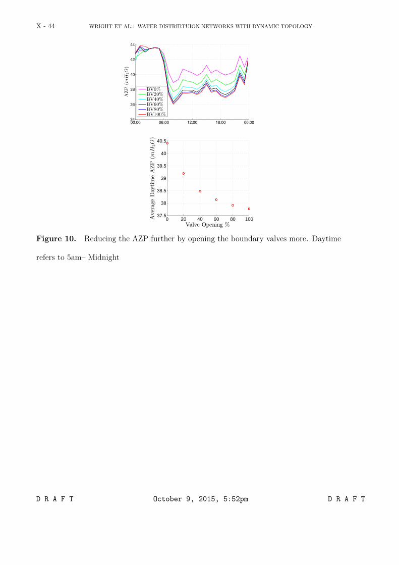
X - 32 WRIGHT ET AL.: WATER DISTRIBTUION NETWORKS WITH DYNAMIC TOPOLOGY

optimization method alone, AZP reductions of up to 6.5% can be achieved when opening568

the boundary valves fully to 100% as shown in Figure 10.569

5. Conclusion

Water companies are becoming increasingly committed to improving customer service570

levels and further reduce leakage. Whilst fixed topology DMAs have helped them to571

identify leakage hotspots, a permanent reduction in network redundancy has resulted in572

reduced resilience to failure, suboptimal pressure management, and water quality con-573

cerns. Operating a dynamic DMA topology is a novel approach towards leakage and574

pressure management that can address these drawbacks whilst still retaining the success575

in identifying and reducing leakage that fixed topology DMAs have facilitated.576

The novel contributions of this paper can be summarised as follows:577

The optimal control of a WDN with dynamic DMA topology is a valve control problem.578

Since the dynamic aggregation of DMAs can result in very large and complex network579

models forming, convergence problems can be caused that are not present when smaller,580

more simple networks are optimized. This paper addresses these convergence problems581

by developing a novel optimization algorithm based on strictly feasible sequential convex582

programming that minimizes AZP. By guaranteeing feasibility at each iteration step,583

reliable convergence could be achieved. The method made use of a null space hydraulic584

algorithm to improve computational efficiency.585

The optimized valve control was successfully actuated in a real, operational WDN operat-586

ing with a dynamic DMA topology. This unique experimental programme demonstrated587

the successful implementation of the novel dynamic DMA topology concept.588

D R A F T October 9, 2015, 5:52pm D R A F T

WRIGHT ET AL.: WATER DISTRIBTUION NETWORKS WITH DYNAMIC TOPOLOGY X - 33

A reduction in AZP of 2.8% was observed experimentally when operating a dynamic DMA589

topology over a closed, static DMA topology. Over a 5 day period, a 5% reduction in590

DMA water input was observed, equivalent to 1Ml of water. It is estimated in simulation591

that opening the boundary valves to 100% will result in an AZP reduction of 6.5%.592

Further analytical and experimental research is required in control optimization, mod-593

elling and water quality analysis in order to fully identify the benefits and challenges594

associated with the operation of DMAs with a dynamic topology. This should focus on:595

Long term studies to compare the pressure management of a dynamic topology in com-596

parison to other operational approaches, including a static DMA structure.597

The exploration of other control strategies for the dynamic topology. In this paper, flow598

modulation curves were produced and the DBVs were programmed with an open-loop599

schedule that allows water companies to utilize added redundancy during the day, and600

carry out leakage management at night. Other control strategies include model predictive601

control for the optimal control of PRVs and DBVs. Valve control in failure scenarios is602

also an unexplored research area.603

An investigation into the other benefits of operating a dynamic DMA topology, such604

as water quality and resilience improvements. The resilience investigation can include605

resilience assessments using both hydraulic measures and graph theoretic approaches.606

An investigation into the cost-benefit ratio of the proposed dynamic DMA topology con-607

cept. The requirement for additional equipment for the operation of a dynamic DMA608

topology increases installation and maintenance costs over standard DMA control prac-609

tices. An investigation into the cost savings made from improved network resilience and610

D R A F T October 9, 2015, 5:52pm D R A F T

X - 34 WRIGHT ET AL.: WATER DISTRIBTUION NETWORKS WITH DYNAMIC TOPOLOGY

pressure management needs to be undertaken in order to justify the investment and scal-611

ability of a dynamic DMA topology.612

Acknowledgments. The authors are grateful for the financial support and technical613

expertise of Bristol Water plc and Cla-Val Ltd. The authors also acknowledge the funding614

supplied by the Engineering and Physical Sciences Research Council. The second author615

is supported by the NEC-Imperial Big Data Technologies for Smart Water Networks616

project. More details on algorithm implementation or data can be made available to the617

interested readers by emailing the authors.618

References

Abraham, E., and I. Stoianov (2015), Sparse null space algothims for hydraulica analysis of619

large scale water supply networks, Journal of Hydraulic Engineering, 11 (1), 11111111.620

Armand, H., I. Stoianov, and N. Graham (2015), Investigating the impact of sectorized621

networks on discoloration, Procedia Engineering, 119, 407415.622

Bertsekas, D. (1999), Nonlinear Programming, second ed., Athena Scientific.623

Boyd, S., and L. Vandenberghe (2004), Convex optimization, Cambridge university press.624

Cla-Val (2015a), D22 pilot controller for position, pressure, flow, and modulation control,625

[Online; accessed 20-04-2015].626

Cla-Val (2015b), e-flowmeter for flow measurements based on the vortex shedding phe-627

nomenon, [Online; accessed 20-04-2015].628

Cla-Val (2015c), e-power mp for energy harvesting, [Online; accessed 20-04-2015].629

Committee, A. E. C. A., et al. (1999), Calibration guidelines for water distribution system630

modeling, in Proceedings of the 1999 AWWA Information Management and Technology631

D R A F T October 9, 2015, 5:52pm D R A F T

WRIGHT ET AL.: WATER DISTRIBTUION NETWORKS WITH DYNAMIC TOPOLOGY X - 35

Conference (IMTech), New Orleans, Louisiana.632

Dinh, Q. T., C. Savorgnan, and M. Diehl (2011), Real-time sequential convex program-633

ming for nonlinear model predictive control and application to a hydro-power plant, in634

Decision and Control and European Control Conference (CDC-ECC), 2011 50th IEEE635

Conference on, pp. 59055910, IEEE.636

Drinking Water Inspectorate (2009), Drinking water safety: Guidance to health and water637

professionals.638

Eck, B. J., and M. Mevissen (2012), Valve placement in water networks: Mixed-integer639

non-linear optimization with quadratic pipe friction, in Company Report.640

Eck, B. J., and M. Mevissen (2013), Fast non-linear optimization for design problems on641

water networks, in World Environmental and Water Resources Congress 2013.642

Elhay, S., A. R. Simpson, J. Deuerlein, B. Alexander, and W. H. Schilders (2014), Re-643

formulated co-tree flows method competitive with the global gradient algorithm for644

solving water distribution system equations, Journal of Water Resources Planning and645

Management, 140 (12).646

Fantozzi, M., F. Calza, and A. Lambert (2009), Experience and results achieved in in-647

troducing district metered areas (dma) and pressure management areas (pma) at enia648

utility (italy), in IWA International Specialised Conference Water Loss.649

Farmani, R., D. A. Savic, and G. A. Walters (2004), Exnet benchmark problem for multi-650

objective optimization of large water systems, Modelling and Control for Participatory651

Planning and Managing Water Systems.652

Hoskins, A., and I. Stoianov (2014), Infrasense: A distributed system for the continuous653

analysis of hydraulic transients, Procedia Engineering, 70, 823832.654

D R A F T October 9, 2015, 5:52pm D R A F T

X - 36 WRIGHT ET AL.: WATER DISTRIBTUION NETWORKS WITH DYNAMIC TOPOLOGY

i2O (2014), Advanced pressure management, [Online; accessed 05-06-2014].655

Jowitt, P. W., and C. Xu (1990), Optimal valve control in water-distribution networks,656

Journal of Water Resources Planning and Management, 116 (4), 455472.657

Lalonde, A., C. Au, P. Fanner, and J. Lei (2008), City of toronto water loss study and658

pressure management pilot, Miya Arison Group, unpublished.659

Luenberger, D. G., and Y. Ye (2008), Linear and nonlinear programming, vol. 116,660

Springer Science & Business Media.661

Ni, Q., C. Zillober, and K. Schittkowski (2005), Sequential convex programming methods662

for solving large topology optimization problems: implementation and computational663

results, Journal of Computational Mathematics -International Edition-, 23 (5), 491.664

Nicolini, M., and L. Zovatto (2009), Optimal location and control of pressure reducing665

valves in water networks, Journal of water resources planning and management, 135 (3),666

178187.667

Nocedal, J., and S. J. Wright (2006), Numerical optimization, Springer Verlag.668

Ofwat (2007), Security of supply 2006-07 report, [Online; accessed 05-06-2014].669

Ofwat (2008), The guaranteed standards scheme (gss), [Online; accessed 15-03-2015].670

Ofwat (2012), The service incentive mechanism (sim), [Online; accessed 05-06-2014].671

Ofwat (2014), Setting price controls for 2015-20 pre-qualification decisions, [Online; ac-672

cessed 23-04-2015].673

Palmer (2015), Pressure control, [Online; accessed 15-03-2015].674

Piller, O., B. Bremond, and M. Poulton (2003), Least action principles appropriate to675

pressure driven models of pipe networks, in ASCE Conf. Proc. 113, pp. 1930.676

D R A F T October 9, 2015, 5:52pm D R A F T

WRIGHT ET AL.: WATER DISTRIBTUION NETWORKS WITH DYNAMIC TOPOLOGY X - 37

Quoc, T. D., C. Savorgnan, and M. Diehl (2012), Real-time sequential convex program-677

ming for optimal control applications, in Modeling, Simulation and Optimization of678

Complex Processes, pp. 91102, Springer.679

Schittkowski, K., and C. Zillober (2005), Sqp versus scp methods for nonlinear program-680

ming, in Optimization and Control with Applications, pp. 305330, Springer.681

Skworcow, P., B. Ulanicki, H. AbdelMeguid, and D. Paluszczyszyn (2010), Model predic-682

tive control for energy and leakage management in water distribution systems.683

Technolog (2014), Regulo, [Online; accessed 05-06-2014].684

Todini, E., and S. Pilati (1988), A gradient algorithm for the analysis of pipe networks,685

in Computer applications in water supply: vol. 1systems analysis and simulation, pp.686

120, Research Studies Press Ltd.687

Ulanicki, B., A. Zehnpfund, and F. Martinez (1996), Simplification of water distribution688

network models, in Proc., 2nd Int. Conf. on Hydroinformatics, pp. 493500, Balkema689

Rotterdam, Netherlands.690

Ulanicki, B., P. Bounds, J. Rance, and L. Reynolds (2000), Open and closed loop pressure691

control for leakage reduction, Urban Water, 2 (2), 105114.692

Vairavamoorthy, K., and J. Lumbers (1998), Leakage reduction in water distribution693

systems: optimal valve control, Journal of hydraulic Engineering, 124 (11), 11461154.694

World Health Organization (2004), Design and operation of distribution networks.695

Wright, R., I. Stoianov, P. Parpas, K. Henderson, and J. King (2014), Adaptive water696

distribution networks with dynamically reconfigurable topology, Journal of Hydroinfor-697

matics, 16 (6), 12801301.698

D R A F T October 9, 2015, 5:52pm D R A F T

X - 38 WRIGHT ET AL.: WATER DISTRIBTUION NETWORKS WITH DYNAMIC TOPOLOGY

Yazdani, A., R. A. Otoo, and P. Jeffrey (2011), Resilience enhancing expansion strategies699

for water distribution systems: A network theory approach, Environmental Modelling700

& Software, 26 (12), 15741582.701

D R A F T October 9, 2015, 5:52pm D R A F T

WRIGHT ET AL.: WATER DISTRIBTUION NETWORKS WITH DYNAMIC TOPOLOGY X - 39

30 40 50 60 7020

30

40

50

60

70

80

90

Total Consumption (l/s)

TotalHeadLoss

(mH

2O)

Single InletMultiple Inlets

Figure 1. A comparison of head losses at various consumption levels (i.e. stochastic

changes in customer demand) for a single and multiple inlet WDN

DMA

Boundary

Large

CustomerHospital

Hospital

DBV 1

CP 1

DMA 1 Inlet

DMA 2

Inlet

PRV 1

DBV 2

Elevation (m)

CP 2

(Tall Building)

PRV 2

Figure 2. Case study description and elevation plot (m)

D R A F T October 9, 2015, 5:52pm D R A F T

X - 40 WRIGHT ET AL.: WATER DISTRIBTUION NETWORKS WITH DYNAMIC TOPOLOGY

Figure 3. (a) A PRV retrofitted with modulating pilot, turbine for energy harvesting,

and antenna for remote comms.(b) Kiosk with real-time pressure and flow communications

sampling at 128S/s

(a)0 20 40 60

0

10

20

30

40

50

60

for PRV 2 (mH2O)

forPRV

1(m

H2O)

Search space minimizing AZP (mH2O)

30

35

40

45

50

55

(b)0 20 40 60

0

10

20

30

40

50

60

for PRV 2 (mH2O)

forPRV

1(m

H2O)

Search space minimizing AZP (mH2O)

30

35

40

45

50

55

Figure 4. (a) Cycling in convergence in an infeasible area, (b) Strictly feasible steps to

aid convergence

D R A F T October 9, 2015, 5:52pm D R A F T

WRIGHT ET AL.: WATER DISTRIBTUION NETWORKS WITH DYNAMIC TOPOLOGY X - 41

(a)00:00 06:00 12:00 18:00 00:000

20

40

60

80

Pressure

Head(m

H2O)

0

5

10

15

20

25

Flow

(l/s)

InletOutletFlow

(b)00:00 06:00 12:00 18:00 00:000

20

40

60

80

Pressure

Head(m

H2O)

0

2

4

6

8

10

12

14

Flow

(l/s)

(c)00:00 06:00 12:00 18:00 00:0025

26

27

28

29

30

Pressure

Head(m

H2O)

0

1

2

Flow

(l/s)

(d)00:00 06:00 12:00 18:00 00:000

10

20

30

40

50

60

70

Pressure

Head(m

H2O)

0

1

2

3

4

5

Flow

(l/s)

Figure 5. Simulated pressure and flow at (a) PRV 1 (b) PRV2 (c) DBV 1 and (d) DBV

2 for the optimal operation of a dynamic DMA topology

D R A F T October 9, 2015, 5:52pm D R A F T

X - 42 WRIGHT ET AL.: WATER DISTRIBTUION NETWORKS WITH DYNAMIC TOPOLOGY

(a)0 10 20 30

5

10

15

20

25

Valve Flow (l/s)

Outlet

Pressure

(mH

2O)

Optimization pointFitted FM curve

(b)0 5 10 15 20

25

25.2

25.4

25.6

25.8

26

26.2

26.4

Valve Flow (l/s)

Outlet

Pressure

(mH

2O)

Figure 6. Fitting of flow modulation curves to the optimization results for (a) PRV 1

and (b) PRV 2

0 10 20 305

10

15

20

25

Valve Flow (l/s)

Outlet

Pressure

(mH

2O)

PRV DataFM Curve

Figure 7. Validation of control actuation at PRV 1 using the acquired pressure data

D R A F T October 9, 2015, 5:52pm D R A F T

WRIGHT ET AL.: WATER DISTRIBTUION NETWORKS WITH DYNAMIC TOPOLOGY X - 43

00:00 06:00 12:00 18:00 00:008

10

12

14

16

18

20

22

Pressure

Head(m

H2O)

Model (Open Loop)Model (FM)Data

Figure 8. Validation of the hydraulic model and optimization using pressure data at

CP 1

01 02 03 04 05 060

5

10

15

20

Day

DMA

Input(106litres)

Closed TopologyDynamic Topology

Figure 9. Comparison of water input over a 5 day period for a closed DMA topology

with flow modulating PRVs and a dynamic DMA topology

D R A F T October 9, 2015, 5:52pm D R A F T

X - 44 WRIGHT ET AL.: WATER DISTRIBTUION NETWORKS WITH DYNAMIC TOPOLOGY

00:00 06:00 12:00 18:00 00:0034

36

38

40

42

44

AZP

(mH

2O)

BV0%BV20%BV40%BV60%BV80%BV100%

0 20 40 60 80 10037.5

38

38.5

39

39.5

40

40.5

Average

DaytimeAZP

(mH

2O)

Valve Opening %

Figure 10. Reducing the AZP further by opening the boundary valves more. Daytime

refers to 5am Midnight

D R A F T October 9, 2015, 5:52pm D R A F T