controllers for nonlinear processes

Synthesis of FeedforwardIState Feedback Controllers for Nonlinear Processes

A systematic method for synthesizing feedforward/ state feedback controllers for a broad class of SISO nonlinear systems with measurable disturbances is presented. Depending on the structural characteristics of the system, the control law can be static or dynamic. The closed-loop system is independent of the measurable disturbances and linear with respect to set point changes. The performance of the proposed control scheme is illustrated through an example of composition control in a system of three CSTR's in series.

Introduction A major problem in the area of chemical process control is the

nonlinear nature of the dynamic behavior of many processes. In the case of mild nonlinearities, linear control techniques, based on a linear approximation of the system, may provide satisfactory performance. There is an increasing demand, however, for nonlinear control strategies, which are able to deal with severe process nonlinearities. The purpose of the present work is to pose and analytically solve the problem of feedforward/feedback control of SISO (single input/single output) nonlinear systems with measurable disturbances.

Recent trends in the area of nonlinear process control are dominated by attempts to calculate a control law that could force the system to follow a prescribed trajectory. From an input/output point of view, calculation of the appropriate manipulated input involves solution of a nonlinear operator equation. Economou et al. (1986) formulated a nonlinear version of I MC (internal model control) and proposed the use of numerical methods for calculating the model inverse on-line. In the same vein, Parrish and Brosilow (1 988) formulated a nonlinear version of inferential control. On the other hand, differential geom- etry has provided an extremely useful mathematical framework for dealing with nonlinear systems, taking into account their internal state-space structure. In this framework, two ap- proaches have prevailed. The Su-Hunt-Meyer method, originally proposed by Su (1982) and Hunt et al. (1983) and applied to chemical engineering systems by Hoo and Kantor (1985) and Kantor (1986), transforms the state-space description of the nonlinear system into a linear one. The inputloutput linearization method (Kravaris and Chung, 1987) develops a state feedback control law that provides linearity of the closed-loop system in an input/output sense.

The use of measurements of the disturbances in a feedfor-

Prodromos Daoutidis Costas Kravaris

Department of Chemical Engineering University of Michigan Ann Arbor, MI 48109

ward/feedback control structure has been recognized as an important problem in nonlinear process control and received increasing attention recently. Bartusiak et al. (1988) provided analytical expressions for feedforward/feedback control laws that force first- and some second-order nonlinear systems to follow a prespecified trajectory. In the context of the Su-Hunt- Meyer method, Calvet and Arkun (1988) proposed a way of adding feedforward control action that eliminates the effect of measurable disturbances, where the disturbances and the manipulated input enter the state-space model through the same scalar function. In addition to the restriction on the class of measurable disturbances, this approach is also limited by the extremely restrictive involutivity condition that has to be satis- fied for the disturbance-free part of the model.

In this work, we will address the general feedforward/feedback control problem for nonlinear SISO systems of arbitrary order, and we will calculate control laws that lead to elimination of the effect of measurable disturbances and a t the same time provide linearity of the closed-loop system with respect to set point changes in an input/output sense. We will start with the problem formulation and we will then provide a characterization of the nonlinear system based on the dynamic effect of the disturbances on the process output. The development of the proposed feedforward/feedback control law will then follow. The stability of the closed-loop system will be discussed next, and the overall control structure will then be completed. Finally, the controller performance characteristics will be illustrated through an example of composition control in a system of three CSTR's (continuous stirred tank reactors) in series.

Problem Formulation The purpose of the synthesis methodology to be presented is to

provide a systematic control framework for a general class of

1602 October 1989 Vol. 35, No. 10 AIChE Journal

DISTURBANCES

Figure 1. Desired control configuration.

SET-POINT - CONTROLLER

SISO nonlinear systems with measurable disturbances. More precisely, we will consider nonlinear systems with state-space representation of the form:

INPUT NONLINEAR STATES OUTPUT OUTPUT PROCESS @ MAP

.

3 = f ( x ) + g ( x ) u + wi(x)di I

wheref, g, wi are vector fields on R", h is a scalar field on R", u is the manipulated input, x is the n-vector of states, dls are measurable disturbances and y is the process output. For the above general class of nonlinear systems, one can state the feedforward/feedback control problem as follows:

Calculate a feedforwardlfeedback control law

where x, y and di are measurements of the states, the output and the disturbances and Y , ~ is the set point, such that:

The output y is completely unaffected by the measured disturbances dp

The input/output behavior of the closed-loop system for changes in y , has desirable performance characteristics.

Figure 1 shows the nonlinear system and the desired control configuration. In order to attack the feedforward/feedback problem, we propose the following two-step formulation, which

will lead to a corresponding two-step control methodology: Step 1. Calculate a feedforward/state feedback control law

that completely eliminates the effect of measured disturbances and provides linear input/output behavior.

Step 2. Use an external linear controller with integral action so that the closed-loop system obtains desired servo and regulatory behavior, despite the presence of unmeasured disturbances and/or modeling errors. In Step 1, which is the main synthesis problem, we will request the following input/output behavior of the closed-loop system:

d'Y ED,- = u dt'

where /?is are adjustable parameters and u is an external input. The solution of this synthesis problem will be developed in the following sections, resulting in a control law of the form:

U = P ( X ) + q ( x ) [ v - W x , d i ) l

where p and q are algebraic functions of the states, and D is in general a nonlinear operator applied on the states and the disturbances that may include time derivatives. This means that the control law will consist of a pure state feedback element and a feedforward state-dependent element, allowing for either static or anticipatory control action. The overall control structure that results from the proposed two-step methodology is depicted in Figure 2.

AIChE Journal

Figure 2. Structure of the proposed control configuration.

October 1989 Vol. 35, No. 10 1603

Remark I. Note that the requirement of linear closed-loop behavior is by no means restrictive. As will be shown later, any nonlinear closed-loop response can be achieved. It is the linear dynamics, however, that we can better understand and for which we can more conveniently express performance specifications.

Structural Characterization of a Nonlinear System with Disturbances

In this section, we will propose an extension of the concept of relative order of the process output with respect to the manipulated input, to include disturbance inputs as well. This extension will allow for a characterization of the dynamic interactions between the process inputs and the output, and will also provide a key conceptual tool in addressing the synthesis problem posed in the previous section. In particular, for the system described by Eq. 1, we define:

r, the relative order of the output with respect to the manipulated input, as the smallest integer for which:

L&;-'h(x) # 0 (2)

p i , the relative order of the output with respect to the disturbance input di, as the smallest integer for which:

(3)

Remark 2. The definition of r is identical to the one originally suggested by Hirschorn ( 1979) for disturbance-free nonlinear systems. The definition of pi is a natural extension of the concept to a disturbance input.

In linear systems, the relative order is equal to the difference between the degrees of the denominator and the numerator polynomials of the transfer function. In general, the relative order of the output with respect to an input is equal to the low- est-order derivative of the output that explicitly depends on that input. Equivalently, it is equal to the number of integrations that the input has to go through before it affects the output. It therefore provides a measure of how direct is the dynamic effect of the input on the output. Thus, by comparing the magnitudes of r and pi, one can determine which input, the manipulated u or the disturbance di, has more direct effect on the process output. Consequently, one should intuitively expect a different nature of the feedforward/feedback control problem, depending on the relation among the various relative orders. Based on the above arguments, the following classification of the disturbances seems meaningful:

Referring to the nonlinear system given by Eq. 1, we define three classes of disturbances, A, B, @, with the properties:

d i e B - p i = r

d i g @ - p i i r

Development of the FeedforwardIFeedback Control Law

In this section, we will provide the solution to the synthesis problem posed in Step 1 of the proposed methodology: the calcu-

lation of a feedforward/feedback control law that eliminates the effect of measured disturbances on the process output and a t the same time provides inputloutput linearity. The nature of the feedforward/feedback compensation term for each disturbance d, will depend on the class this disturbance belongs to. In particular, in the special case of one disturbance with corresponding relative order equal to p, the necessary feedforward/feedback law will turn out to be:

ifd E A

i f d E 23

It is clear that when d E A, the disturbance effect is less direct than the manipulated input effect on the process output. For this reason, no feedforward compensation is necessary. All the useful information on how the disturbance changes can be found in the process states. On the other hand, when d €23, both the disturbance and the manipulated input affect the output in the same way. Therefore, a feedforward/state feedback element which is static in the disturbance is necessary in the control law in addition to the pure state feedback element. Finally, when d E @, the disturbance affects the output more directly than the manipulated input. Consequently, effective control must involve anticipatory action for the disturbance. Indeed, the control law in this case has a dynamic feedforward/state feedback component which differentiates a state- and disturbance-dependent signal up to r - p times, in addition to the pure static state feedback component. The dynamic element can be implemented in the customary way, i.e., using a lead-lag type of approximation of appropriate order.

In the general case of the system described by Eq. 1, under the combined effect of all the disturbances di, one must compensate for them in the control law in a way that depends on the relative magnitude of the corresponding relative orders. The general result is presented in the following theorem:

Theorem. For the nonlinear system described by Eq. 1, let r , p i the relative orders as defined by Eq. 2, Eq. 3, and A, 8, @ the classes of disturbances defined by Eq. 4. Then, the feedforward/ feedback control law that

Makes y independent of d;s Makes y linearly dependent on an external input u through

dJy dtJ

xpj- = u,


is given by:

Proof: Let p* be the minimal relative order pi of the output with respect to the disturbances in class 6). Also, define the following subclasses of class e:

Then, we can calculate the derivatives of the output as follows:

Y = h ( x )

2 = L,h(x) dt

d + ~i ; (L ,L ; - ' h (x )d , ) ] + . . .

d'y = Ljh(x) + L,L;-'h(x)u dt

d + ~ ( L , , L ; - ~ h ( x ) d i ) ] + * *

Using the above expressions to form the sum

and substituting u from Eq. 6, we easily find after some algebraic manipulations:

which completes the proof. It is clear from Eq. 6 that the feedforward/state feedback control law is composed of

A pure state feedback part, which is static in nature

I

vFB - 1 ~ , ~ j h ( x )

P,LgLj- ' h ( x ) (7)

1-0 U =

A feedforward/state feedback part, which in general involves anticipatory action

These two parts are clearly depicted as two separate compensa- tors in the control configuration of Figure 2.

Remark 3. Under the proposed control law (Eq. 6), the order of the closed-loop input/output system is equal to r, i.e., the

AlChE Journal October 1989 Vol. 35, No. 10 1605

input/output behavior of the v - y system is described by:

(9)

This arises as a natural consequence of the definition of the relative order r; it is necessary to differentiate the output at least r times so that the manipulated variable can appear explicitly in a nonsingular fashion.

Remark 4. Following the procedure outlined in the proof of the Theorem, it is possible to calculate the control law for any desired nonlinear disturbance-free closed-loop behavior of the form:

Such an extension, however, does not seem particularly meaningful.

Remark 5. Hirschorn (1981) and Isidori et al. (1981) formulated and solved the disturbance decoupling problem for nonlinear systems, i.e., the problem of calculating a static pure state feedback control law such that the output in the closed-loop system is not affected by the disturbances. They showed that the necessary and sufficient condition for solvability of this problem is:

wi(x) E kerdh(x) n . , . (7 kerdLj-'h(x).

It can be easily shown (Daoutidis and Kravaris, 1989) that, expressing the above condition in terms of relative orders, yields, as expected, the condition pi > r. The latter condition is, of course, much simpler and more transparent. Moreover, our feedforward/feedback formulation is more general than the disturbance decoupling formulation, and therefore leads to more general results, namely elimination of the effect of a larger class of measured disturbances (disturbances for which pi - r or pi c r ) on the process output.

Stability of the Closed-Loop System The BIBO (bounded input/bounded output) stability charac-

teristics of the closed-loop system under the proposed control law (Eq. 6 ) . depend on the location of the roots of

D o + BJ + 8*s2 + - * ' +B,S = 0.

Since the parameters 8;s are adjustable, they can always be chosen for closed-loop input/output stability and fast dynamics.

In addition to the input/output stability characterization, one must also obtain a characterization for the closed-loop asymptotic stability of the states, under no external input. In the case of a disturbance-free system and in the context of the input/output linearizing control methodology (Kravaris and Chung, 1987), this would be equivalent to characterizing the internal stability of the closed-loop system, i.e., the asymptotic stability of the states with respect to perturbations in the initial conditions. Such a characterization has been obtained (Kravaris, 1988) by using the concept of zero dynamics of Byrnes and Isi- dori (1985). In the case of a nonlinear system with disturbances,

a characterization of the asymptotic stability of thestates will be of more general nature, including stability with respect to the disturbance inputs, as well as internal stability of the system. Such a characterization will be obtained through a concept analogous to the zero dynamics of the disturbance-free system.

At first, one must observe that when the system described by Eq. 1 is subject to the control law (Eq. 6), the output dynamics of the unforced closed-loop system is governed by:

' dJy j - 0 dtl z p . - = 0 ,

under appropriate initial conditions. Thus, by choosing the adjustable parameters @ i s so that the closed-loop system is BIBO stable, any initial conditions of the states will generate exponentially decaying signals for the output y and its derivatives dyldt , . . . , ( d r - ' y ) / d f - ' . Moreover, the output and its derivatives will get arbitrarily close to zero in finite time. Conse- quently, the asymptotic stability of the states (i.e., the stability as t - m) of the unforced closed-loop system will depend, for all practical purposes, on the asymptotic stability characteristics ofthe dynamical system resulting when y ( t ) = [ d y ( t ) ] / dt = - - - = [d'-'y(t)]/dt'-' = 0. In a disturbance-free system, this dynamical system is exactly the zero dynamics of Byrnes and Isidori, which conforms with the intuitive interpretation of the zeros in terms of the block transmission property.

The above arguments motivate an extension of the concept of zero dynamics for systems with disturbances. In particular, the zero dynamics of the system described by Eq. 1 is defined as its dynamics when the output is constrained to be equal to zero for all times. The asymptotic stability properties of the zero dynamics, with respect to the disturbances and the initial conditions, will completely characterize the asymptotic stability of the states of the unforced closed-loop system. In what follows, we will introduce a normal form for a nonlinear system with disturbances through the Byrnes-Isidori coordinate transformation, and we will use it to obtain a representation of the zero dynamics.

For a nonlinear system with relative order of the output with respect to the manipulated input equal to r, Byrnes and Isidori (1985) introduced the following transformation

where

are linearly-independent scalar fields, i = 1, . . , , (n - r )

and used it to obtain a normal form for a disturbance-free non-

t ' ( X ) , . . , , L ( X ) , h(x) , Lfh(X), . . . , Lj-*h(x), Lj-'h(x)

* L g t i ( x ) = 0,

AIChE Journal 1606 October 1989 Vol. 35, No. 10

linear system, which is the nonlinear analog of the output con- trollability canonical form of disturbance-free linear systems.

Consider first the case where only disturbances that belong to classes dl and B are present. Then, the system described by Eq. 1 under the coordinate transformation (Eq. 10) becomes:

L, = t" r, = L;h(t) + L&-'h(f)u + E Lw,L;-'h(f)di

d,E p1

Y = {"-,+I (11)

In this new system representation, it is clear how the various disturbances enter the system and affect the output. In particular,

Disturbances of class .A enter the system only through the first n - r state equations. The first n - r state variables in turn affect the righthand side of the last state equation and finally through a chain of r integrations, the output y = fn-r+l.

The effect of disturbances of class B is similar, except that they also affect the righthand side of the last state equation in a direct way. Referring to the new system representation given by Eq. 11, the conditions

imply:

Consequently, the zero dynamics of the system described by Eq. 1 is given by:

pletely characterize the asymptotic stability of the unforced closed-loop system. It is interesting to note that Eq. 12 reduces to the standard zero dynamics of Byrnes and Isidori, in a disturbance-free situation (di - 0).

In the general case where disturbances that belong to class 8 are also present, the system (Eq. 1) under the coordinate transformation (Eq. 10) takes the form:

L,+I = L r + *

7 -I h (t) di

Y = {"-,+I

where p* and @ ( I ) , G'(2), . . . , are as defined in the proof of the Theorem.

In this system representation, it is easy to see that the effect of disturbances of class 8 on the output y = is much more direct compared with that of the disturbances of classes .A and 8. Disturbances of class 6 affect not only the last state equation but also some of the previous state equations and, therefore, have to go through a smaller number of integrations before they affect the output y . Imposing the zero-output conditions in the above system representation, we obtain the zero dynamics of the system of Eq. 1 as the dynamical system:

!L = L,t,_,(SI,. . . , L,, 0,. . . ,O)

+ E ~w,t"-,(tl, . . . , t n - r , 0, . * . , O M (12) d, E A,¶

The asymptotic stability characteristics of this system with respect to the disturbances and the initial conditions, will com-

(14)

1607 AIChE Journal October 1989 Vol. 35, No. 10

subject to the constraints:

f n - r + i - 0

L + Z - 0

i n - r + p . = 0

Obtaining algebraic expressions for the last r - p* state variables in terms of j-,, . . . , Cn-,, di and the derivatives of di, may not always be possible. The order and the exact state-space real- ization of the zero dynamics will depend on the specific nonlinear system (Q. 1). When no disturbances di are present, the zero dynamics defined above reduces to the standard zero dynamics of Byrnes and Isidori, as expected.

The External Controller After solving the main synthesis problem and obtaining a sta-

bility characterization of the closed-loop system, the second step of the proposed methodology is the tuning of a linear controller with integral action around the linear u - y system, which will reject the effect of modeling errors and/or unmeasured disturbances. For example, one can use a PI controller:

In this case, the overall closed-loop BIB0 stability depends on the location of the roots of the characteristic equation:

Kc ( P o + K , ) + - + @IS + &s2 + - * * + PP' = 0

71 s

The General FeedforwardlFeedback Synthesis Algorithm

consisting of the following steps: Given the system model

To summarize, we could describe the proposed algorithm as

1 = f ( x ) + g(x)u + W i ( X ) d ,

Y - 1. Calculate L,L$h(x) and L,L?h(x) until # 0, identifying

2. (a) Compute the control law from Eq. 6; (b) select @ to thus the relative orders rand pi.

place the roots of

sufficiently far left in the complex plane. 3. Tune an external linear controller which possesses integral

action (e.g., a PI controller). Remark 6. In the case of no measurable disturbances or all

measurable disturbances belonging to class A, the control law (Eq. 6) becomes

The overall control configuration will be as in Figure 2, except that the feedforward/feedback compensator will be missing. In other words, the proposed control structure reduces to the Glob- ally Linearizing Control (GLC) structure (Kravaris and Chung, 1987).

Remark 7. Consider the class of nonlinear processes of the form:

where +(x, u, d * ) is a scalar function solvable for u and d * is a vector of disturbances. This is a more general class of systems than the one described by Eq. 1. The proposed methodology can be applied by simply letting 4(x, u, d * ) = "u, calculating "u as proposed by Eq. 6 and solving for the actual manipulated input u. In this way, compensation for the disturbances d* is also possible.

Evaluation of the Controller Performance: Simulations

The efficacy of the proposed algorithm will be demonstrated through an example of composition control of a system of 3 CSTRs in series, where a second-order reaction A - B is taking place. Figure 3 provides a schematic description of the system. It is desired to maintain the composition of the stream leaving the

October 1989 Vol. 35, No. 10 AIChE Journal 1608

Figure 3. System of three CSTR's in series.

last reactor constant, despite fluctuations in the feed temperature and /or composition.

Three cases are examined: Case I . The major disturbances are the inlet concentration

and temperature, and the manipulated input is the heat input in the third vessel.

Case 2. The major disturbance is the inlet temperature, and the manipulated input is the heat input in the first vessel.

Case 3. The major disturbance is the inlet concentration, and the manipulated input is the heat input in the first vessel.

The purpose of this example is to illustrate the proposed control methodology for the various cases and explain the nature of the necessary feedforward compensations rather than to propose the best choice of manipulated input. Although Cases 2 and 3 could be examined together, we choose to examine them sepa- rately for methodological reasons.

We assume that both heating and cooling of the reactors are possible. We also assume that the inlet and intermediate flow rates, as well as the reactor volumes, are equal and remain constant during the operation. The dynamic equations of the system are the mass and energy balances for each reactor, and the form they take under the previous assumptions is:

dCA 1 V - = F(cA0 - c A l ) - Vk,c:l dt

dCA3 v- = F ( C A , - C A 3 ) - Vk3Ci3 dt

The following typical values were given to the process parameters:

F - 54, V = 9, E = 76,480, ko - 1.25 x lOI4, A H - -500 x lo3, pc, - 30,000

The steady-state values of the process variables were:

To - 298.13,

cA0 = 2.1641, c,,, - 1.1216, cA, = 0.7071, cA3, * 0.5

TI , - T, - T3, = 298.13,

These conditions correspond to a stable steady state as it was

AIChE Journal October 1989 Vol. 35, No. 10 1609

t Figure 4. Interaction paths among process variables:

Case 1.

verified by the simulations. The states of the system are chosen to be the concentrations and temperatures in each reactor,

all assumed measurable. Figures 4, 5 and 6 describe the interactions among the process variables and the properties of each structure for the following cases:

0 Case 1 , As shown in Figure 4 and can be easily seen from the system dynamic equations, the disturbances and the manipulated input affect the output through different paths. A change at To has to go through three more states before affecting the output (e.g., To - T , - T2 - T, - y). The path is shorter for cAo, for which only two states are affected before the output (cAo - c,, - cA2 - y). The manipulated input, on the other hand, causes the change of only one state (T,) before the output. Moreover, since both the manipulated and the controlled variables are in the third tank, the effect of any of the disturbances is actually transferred to the states cA2 and T2. Therefore, no mea- surement of the disturbances is required provided that the states are measured.

1 u= Q I

Figure 6. Interaction paths among process variables: Case 3.

Case 2. Figure 5 shows clearly that both inputs (the disturbance To and the manipulated input Q , ) immediately affect TI and then two more states before they affect the output. Physi- cally, the effects of To and QI are very similar and a change A To can be eliminated by a change AQ, - - Fpc,A T,.

Case 3. Figure 6 reveals a very interesting property of this system. The shortest path, that a change at the disturbance cA0 must follow in order to reach the output, involves two intermediate states (cAi and cAz), while the one for the manipulated input QI involves three (e.g., T,, c,,, and cA2). Therefore, the disturbance has a more direct effect on the output than the manipulated input, and it is expected that predictive action will be necessary to eliminate the effect of the disturbance.

All the above arguments are based mostly on intuition and a physical understanding of the process. The mathematical approach, using the defined concepts of relative order, results in exactly the same conclusions about the nature of the control law. In addition, we will see that the relative order with respect to an input is equal to the number of intermediate states affected by this input, including the output.

To evaluate the controller performance, we tested: 1. The ability of the closed-loop system to reject disturbances

(regulatory behavior). 2. The ability of the closed-loop system to follow set point

changes (servo behavior). For the two disturbances considered, step changes and random noise were applied. In the simulated noise, we used a standard deviation of 0.5 for the concentration and 20 for the temperature. The step inputs were 2.5 and 308 respectively, and they were applied at TIME = 0.5. Since no model uncertainty or unmeasured disturbances were considered, the external PI loop of the control scheme remained inactive. The performance of the FF/FB (feedforward/feedback) control scheme was compared with that of GLC, which does not use measurements of the disturbances in the control law.

Case I Defining

Figure 5. Interaction paths among process variables: Case 2.

1610 October 1989 Vol. 35, No. 10

11 = Q, d , = To

d2 = cAO

AIChE Journal

the state equations can be put in the form of Q. 1, where

- I -

VPCp

0

0

0

0

0

Case 2 Defining

, w ( x ) =

'F AH

PCP

, ( - X I ) - - k k , x i + -

- F V

0

0

0

0

-

0,

u = QI d - To

the newf; g and w functions are:

F AH - ( - X I ) - - k l x ; V PCP

J F AH Q3 - (x3 - XJ - - k3x: + - V PCP VPCp

F - ( ~ 4 - x S ) - k3x: V

h ( x ) = X 6

Following the steps of the proposed algorithm:

1. (a) L,h(x) = 0 L,L/h(X) f 0

L, ,Ljh(x) f 0

L, ,Ljh(x) f 0

(b) L,,h(x) = L,,L/h(x) = L,,Ljh(x) = 0

(c) L,h(x) = L,Lfh(X) = 0

So, r = 2, pI = 4, p 2 = 3

and h ( x ) remains the same. In this case, one proceeds as follows:

1. (a) L,h(x) - L,L,h(x) = L,Ljh(x) = 0 L,LpI(x) # 0

L,Ljh(x) z 0 (b) L,h(x) - L,L/h(x) = L,L jh(x ) = 0

So, r - p = 4 2. (a)

2

u - PjLjh(X) i-0

(b) We choose B0 = 30,000, - 9,500,& = 1,100,8, = 55, p4 = 1 to place the closed loop poles at - 10, - 10, -15, -20.

(b) We choose Po = 100, PI = 20, Pz = 1 to place the closed-loop poles at - 10, - 10.

Because of the relation among the three relative orders, no feedforward compensation is used in the control law. The behavior of the closed-loop system under this control law is shown in Figures 7 and 8. In Figure 7, the output is not affected under step and noise disturbances, both in cAo and To. In Figure 8, the servo behavior of the closed-loop system is shown under random noise disturbance in cAo and T,. The response is identical with the one obtained when the disturbances are not present.

Figures 9 and 10 illustrate the performance of this static feedforward/feedback control law, comparing it with the performance of GLC, where pure state feedback action is applied and an external PI controller is responsible for the disturbance rejec- tion. In Figure 9, under a step change in the inlet temperature, the open-loop, the FF/FB and the GLC responses are compared. The PI settings in the GLC case were K, - 50,000 and 7, - 0.5. The feedforward compensation improves considerably the regu-


1612

0.56-

O Y -

032 -

0 .u 0 0.t 0.2 0.1 0.4 0 3 0.6 0.7 0.6 0.9 1

TIME

Figure 7. Output response under random or step disturbances: Case 1.

0.55

O Y

0.5.3

* z 032 0

0.Sl

0.49 0 0.1 0.2 0.1 0.4 0.S 0.6 0.7 0.6 0.9 1

TIME

Figure 8. Set point tracking under random noise at the disturbances: Case 1.

October 1989 Vol. 35, No. 10 AIChE Journal

0.50

0.45

0.40

g 0.35

0

0.30

035

0.20

\ 1

\ \

0.15 i 0.5 1 1.1 2

TIME

Legend m p m - w o ~ o w ....... *L

Figure 9. Output response under step change at the disturbance: Case 2.

0.56

0.53 1 0.54

j 0.53

0

0.52

0.51

I f i

0.404 1 0 0.5 1.5 2 2.5 3 1

1

m i E

Legend m. ....

0 W E 5

1613 AIChE Journal

Figure 10. Set point tracking under random noise at the disturbance: Case 2.

October 1989 Vol. 35, No. 10

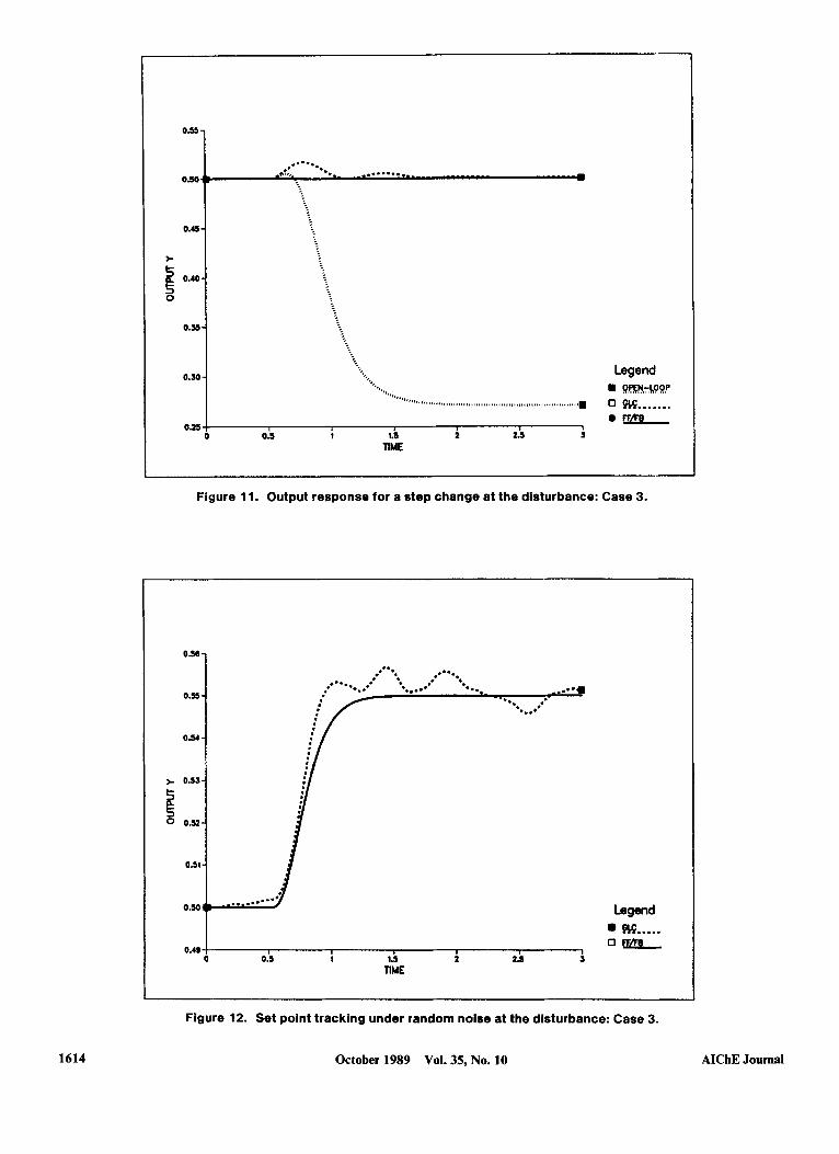
Figure 11. Output response for a step change at the disturbance: Case 3.

0.53

0.55

0.54

+ 0.53

E 0 0.52

0.51

0.49 1 0 0.5 1.5 2 2.5 S

TlME

I 1

Legend m.....

AIChE Journal 1614

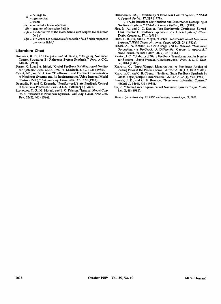
Figure 12. Set point tracking under random noise at the disturbance: Case 3.

October 1989 Vol. 35, No. 10

latory behavior of the system. In Figure 10 the system is forced to track a set-point change a t TIME = 0.5, under noise a t the inlet temperature. The response under the feedforward/feedback action is identical to the one under GLC in the case where no disturbance is present. Under the presence of the disturbance, however, the feedforward action improves considerably the system behavior, as expected. For the PI controller in the GLC structure, we used K, = 5,000 and ri = I .

F ,(-x2> - k , x :

F AH Q2 y ( ~ , - x3) - - k2x: + - VPCP

F - (x2 - x3) - k& V

PCP f(x) =

F AH Q 3

PCP VPCP 7 (x3 - x5) - - k3xi + -

Case 3 Defining

-0 -

F V -

, W ( X ) = 0 (30) 0

0

0

Q i

d = cA0

the new f and w functions are:

J where g and h remain the same as in Case 2. Again, following the algorithm steps:

1. (a) ~ , h ( x ) = ~ , L , h ( x ) = L,Ljh(x) = O L,Ljh(x) f 0

L,Ljh(x) # 0 (b) L,h(x) = L,,,L/h(x) = 0

So, r = 4 and p = 3 2. (a)

(b) We choose 13, = 30,000, PI = 9,500, P 2 = 1,100, P3 =

55, P4 = 1 to place the closed-loop poles a t -10, -10, -15, - 20.

In this case, the control law (Eq. 31) involves the first derivative of the disturbance: i.e., it is dynamic with respect to the disturbance. This is consistent with the intuitive argument made ear- lier, and its mathematical justification is based on the relation between the two relative orders. The derivative action was implemented using a first-order lead-lag approximation with the filter parameter equal to 0.01. Figures 11 and 12 illustrate the

behavior of the system under the same conditions described in Case 2. As expected, the feedforward action improves signifi- cantly the servo and regulatory behavior of the closed-loop system.

Remark 8. In all three cases presented in the example, the corresponding figures do not show any effect of the disturbances on the process output. This happens because the model and measurements are assumed to be perfect, there are no active constraints on the input, and there is not any time lag in the control action.

Conclusions The present work addressed a broad class of nonlinear SISO

systems with measurable disturbances. The concept of relative order, extended to disturbance inputs, was proven to be a very useful tool in characterizing the dynamic structure of the nonlinear system. Analytical expressions for the feedforward/state feedback control law were developed and applied to the control of a reaction system of three CSTR's in series. The proposed methodology was proven to be a very powerful technique in completely eliminating the effect of measured disturbances and pro- viding satisfactory servo behavior.

Notation A, B = reactant and product

A, B, B = classes of disturbances C,, = concentration of species A in the ith reactor, gmol/L

d, = disturbance input E = activation energy, J/gmol F = volumetric feed rate, L/h 3 = control law

g, w, = vector fields h, r , = scalar fields K, = proportional gain k, = specific rate constant, L/gmol . h

Q, = heat input in ith reactor, J/h R = ideal gas constant, J/gmol . K R = real line

R" = n-dimensional Euclidian space

k , , k,, k , = rate constants, L/gmol - h

r = relative order of the output with respect to the manipulated

s = Laplace domain variable input

T, = temperature in the ith reactor, K 'U = generalized manipulated input u = manipulated input V = reactor volume, L v = external input to the inner loop of the control structure x - vector of state variables y = output

ysp = set point

Greek letters @, = parameters of the feedfonvardlstate feedback law

A H = heat of reaction, J/gmol { - transformed state variables

T , = reset time p, = relative order of the output with respect to the disturbance

4 p* = minimal relative order p, for disturbances in class @ pc,, = thermal capacity, J/L . K

Math symbols - = implies c- = is equivalent to


E - belongs to n = intersection U - union

ker - kernel of a linear operator dh - gradient of the scalar field h

L,h - Lie derivative of the scalar field h with respect to the vector

L;h - kth-order Lie derivative of the scalar field h with respect to field f

the vector field f

Literature Cited Bartusiak, R. D., C. Georgakis, and M. Reilly, “Designing Nonlinear

Control Structures By Reference System Synthesis,” Proc. A.C.C., Atlanta (1988).

Byrnes, C. I., and A. Isidori, “Global Feedback Stabilization of Nonlin- ear Systems,” Proc. IEEE CDC, Ft. Lauderdale, FL, 1031 (1985).

Calvet, J-P., and Y. Arkun, “Feedforward and Feedback Linearization of Nonlinear Systems and Its Implementation Using Internal Model Control (IMC),” Ind. and Eng. Chem. Res., 27, 1822 (1988).

Daoutidis, P., and C. Kravaris, “Feedforward/State Feedback Control of Nonlinear Processes,’’ Proc. A.C.C.. Pittsburgh (1989).

Economou, C. G., M. Morari, and 3.0. Pafsson, “Internal Model Con- trol 5: Extension to Nonlinear Systems,” Ind. Eng. Chem. Proc. Des. Dev.. 25(2), 403 (1986).

Hirschorn, R. M., “Invertibility of Nonlinear Control Systems,” SIAM J. Control Optim., 17,289 (1979).

, “(A,B)-Invariant Distributions and Disturbance Decoupling of Nonlinear Systems,” SIAM J. Control Optim., 19, 1 (198 I).

Hoo, K. A., and J. C. Kantor, “An Exothermic Continuous Stirred- Tank Reactor Is Feedback Equivalent to a Linear System,” Chem. Engin. Commun., 37, 1 (1985).

Hunt, L. R., Su, and G. Meyer, “Global Transformations of Nonlinear Systems,” IEEE Trans. Automat. Contr. AC-28,24 (1983a).

Isidori, A., A. Krener, C. Gori-Giorgi, and S. Monaco, “Nonlinear Decoupling via Feedback A Differential Geometric Approach,” IEEE Trans. Autom. Contr., 26(2), 331 (1981).

Kantor, J. C., “Stability of State Feedback Transformation for Nonlin- ear SystemsSome Practical Considerations,” Proc. A. C. C.. Seat- tle, 1014 (1986).

Kravaris, C., “Input/Output Linearization: A Nonlinear Analog of Placing Poles at the Process Zeros,’’ AIChE J.. 34(1 l), 1803 (1988).

Kravaris, C., and C. B. Chung, “Nonlinear State Feedback Synthesis by Global Input/Output Linearization,” AIChE J., 33(4), 592 (1987).

Parrish, J. R., and C. B. Brosilow, “Nonlinear Inferential Control,” AIChE J., 34(4), 633 (1988).

Su, R., “On the Linear Equivalents of Nonlinear Systems,” Syst. Contr. Let.. 2,48 (1982).

Manuscript received Aug. 22. 1988. and revision received Apr. 17, 1989.


controllers for nonlinear processes

Documents