controlling the parallel execution of … · 2. databases. 3. distributed ... agradeço ao...
TRANSCRIPT

CONTROLLING THE PARALLEL EXECUTION OF WORKFLOWS
RELYING ON A DISTRIBUTED DATABASE
Renan Francisco Santos Souza
Dissertação de Mestrado apresentada ao
Programa de Pós-graduação em Engenharia de
Sistemas e Computação, COPPE, da
Universidade Federal do Rio de Janeiro, como
parte dos requisitos necessários à obtenção do
título de Mestre em Engenharia de Sistemas e
Computação.
Orientadora: Marta Lima de Queirós Mattoso
Rio de Janeiro
Julho de 2015

CONTROLLING THE PARALLEL EXECUTION OF WORKFLOWS
RELYING ON A DISTRIBUTED DATABASE
Renan Francisco Santos Souza
DISSERTAÇÃO SUBMETIDA AO CORPO DOCENTE DO INSTITUTO
ALBERTO LUIZ COIMBRA DE PÓS-GRADUAÇÃO E PESQUISA DE
ENGENHARIA (COPPE) DA UNIVERSIDADE FEDERAL DO RIO DE JANEIRO
COMO PARTE DOS REQUISITOS NECESSÁRIOS PARA A OBTENÇÃO DO
GRAU DE MESTRE EM CIÊNCIAS EM ENGENHARIA DE SISTEMAS E
COMPUTAÇÃO.
Examinada por:
Profa. Marta Lima de Queirós Mattoso, D.Sc.
Prof. Alexandre de Assis Bento Lima, D.Sc.
Profa. Lúcia Maria de Assumpção Drummond, D.Sc.
Prof. Daniel Cardoso Moraes de Oliveira, D.Sc.
RIO DE JANEIRO, RJ - BRASIL
JULHO DE 2015

iii
Souza, Renan Francisco Santos
Controlling the Parallel Execution of Workflows
Relying on a Distributed Database / Renan Francisco
Santos Souza. – Rio de Janeiro: UFRJ/COPPE, 2015.
XI, 86 p.: il.; 29,7 cm.
Orientadora: Marta Lima de Queirós Mattoso
Dissertação (mestrado) – UFRJ/ COPPE/ Programa de
Engenharia de Sistemas e Computação, 2015.
Referências Bibliográficas: p. 83-86.
1. Scientific Workflows. 2. Databases. 3. Distributed
Data Management. I. Mattoso, Marta Lima de Queirós II.
Universidade Federal do Rio de Janeiro, COPPE,
Programa de Engenharia de Sistemas e Computação. III
Título.

iv
Agradecimentos
Primeiramente, agradeço a Deus, porque dele, por ele, e para ele são todas as coisas,
inclusive minha vida e este trabalho.
Agradeço ao meu pai, ao Marcos, e, principalmente, à minha mãe. É notória sua
vontade de me apoiar e de me ver crescendo. Agradeço pelos sacrifícios necessários para
investir na minha educação. Tenho plena ciência de que sem sua ajuda, eu não teria
conseguido chegar até aqui e, por isso, serei eternamente grato.
Agradeço à Gisele, minha namorada, por ter sido minha principal motivação por todos
esses anos e por continuar dando um significado maior a todo meu esforço. Também agradeço
a seus pais e irmão pelo apoio e compreensão durante as ausências.
Agradeço à minha professora orientadora Marta Mattoso, de quem eu tenho orgulho
de ser aluno. Agradeço por ter me recebido tão bem em seu grupo de pesquisa, por ter me
ensinado não só técnicas de bancos de dados, mas principalmente a ter uma visão crítica e
analítica para trabalhos científicos, que vão muito além dos detalhes técnicos. Sua dedicação
ao trabalho e seu esforço me inspiram.
Agradeço ao Vítor Sousa, colega, amigo e orientador. Incontáveis pedidos de ajuda
atendidos, nas mais altas horas até de madrugada às vezes, foram essenciais para o
desenvolvimento deste trabalho. Sua orientação bem próxima e, principalmente, seu incentivo
foram determinantes para que eu prosseguisse adequadamente até o fim desta dissertação.
Muito obrigado, como sempre!
Agradeço ao professor Alexandre Lima, de quem eu sou fã, pelas incansáveis trocas
de e-mails, respondidos quase sempre imediatamente, e reuniões até sanar todas minhas
dúvidas, que frequentemente eram muitas. Sua ajuda foi essencial para que eu compreendesse
um problema difícil da minha dissertação, logo, para resolvê-lo também. Obrigado pela
paciência e insistência para que meus trabalhos fiquem sempre melhores. Ah, também
agradeço pelos cabelos brancos que ganhei depois de cursar suas disciplinas :).
Agradeço ao professor Daniel de Oliveira pela colaboração tão próxima e,
principalmente, pela sua dedicação. Também agradeço à professora Kary Ocaña por sua
bondade e palavras de incentivo. Agradeço à professora Maria Luiza Campos pelo carinho e
orientação de sempre. Também agradeço aos professores Cláudio Amorim, Myriam Costa e
Álvaro Coutinho pelas aulas de paralelismo. Agradeço à professora Lúcia Drummond por
aceitar fazer parte da banca desta dissertação.

v
Agradeço a todos os amigos que me apoiam e incentivam, seja com discussões e
ideias para meu trabalho, seja com singelas palavras de incentivo. Sua amizade é muito
importante para mim.
Também agradeço à Mara Prata, Ana Paula Rabello, Solange Santos e Gutierrez da
Costa, pela ajuda nas questões administrativas. Também agradeço à Sandra da Silva pelo
carinho.
Agradeço à CAPES pela concessão da bolsa de mestrado.
Finalmente, agradeço à equipe do NACAD-COPPE/UFRJ e ao professor Patrick
Valduriez (Grid5000) pela ajuda com os equipamentos usados nos experimentos e durante o
desenvolvimento deste trabalho.
A todos, muito, muito obrigado!
vi
Resumo da Dissertação apresentada à COPPE/UFRJ como parte dos requisitos necessários
para a obtenção do grau de Mestre em Ciências (M.Sc.)
GERÊNCIA DA EXECUÇÃO PARALELA DE WORKFLOWS APOIADA POR
UM BANCO DE DADOS DISTRIBUÍDO
Renan Francisco Santos Souza
Julho/2015
Orientadora: Marta Lima de Queirós Mattoso
Programa: Engenharia de Sistemas e Computação
Simulações computacionais de larga escala requerem processamento de alto
desempenho, envolvem manipulação de muitos dados e são comumente modeladas como
workflows científicos centrados em dados, gerenciados por um Sistema de Gerência de
Workflows Científicos (SGWfC). Em uma execução paralela, um SGWfC escalona muitas
tarefas para os recursos computacionais e Processamento de Muitas Tarefas (MTC, do
inglês Many Task Computing) é o paradigma que contempla esse cenário. Para gerenciar
os dados de execução necessários para a gerência do paralelismo em MTC, uma máquina
de execução precisa de uma estrutura de dados escalável para acomodar tais tarefas. Além
dos dados da execução, armazenar dados de proveniência e de domínio em tempo de
execução permite várias vantagens, como monitoramento da execução, descoberta
antecipada de resultados e execução interativa. Apesar de esses dados poderem ser
gerenciados através de várias abordagens (e.g, arquivos de log, SGBD, ou abordagem
híbrida), a utilização de um SGBD centralizado provê diversas capacidades analíticas, o
que é bem valioso para os usuários finais. Entretanto, se por um lado o uso de um SGBD
centralizado permite vantagens importantes, por outro, um ponto único de falha e de
contenção é introduzido, o que prejudica o desempenho em ambientes de grande porte.
Para tratar isso, propomos uma arquitetura que remove a responsabilidade de um nó central
com o qual todos os outros nós precisam se comunicar para escalonamento das tarefas, o
que gera um ponto de contenção; e transferimos tal responsabilidade para um SGBD
distribuído. Dessa forma, mostramos que nossa solução frequentemente alcança eficiências
de mais de 80% e ganhos de mais de 90% em relação à arquitetura baseada em um SGBD
centralizado, em um cluster de 1000 cores. Mais importante, alcançamos esses resultados
sem abdicar das vantagens de se usar um SGBD para gerenciar os dados de execução,
proveniência e de domínio, conjuntamente, em tempo de execução.

vii
Abstract of Dissertation presented to COPPE/UFRJ as a partial fulfillment of the requirements
for the degree of Master of Science (M.Sc.)
CONTROLLING THE PARALLEL EXECUTION OF WORKFLOWS RELYING
ON A DISTRIBUTED DATABASE
Renan Francisco Santos Souza
July/2015
Advisor: Marta Lima de Queirós Mattoso
Department: Systems and Computer Engineering
Large-scale computer-based scientific simulations require high performance
computing, involve big data manipulation, and are commonly modeled as data-centric
scientific workflows managed by a Scientific Workflow Management System (SWfMS). In a
parallel execution, a SWfMS schedules many tasks to the computing resources and Many
Task Computing (MTC) is the paradigm that contemplates this scenario. In order to manage
the execution data necessary for the parallel execution management and tasks’ scheduling in
MTC, an execution engine needs a scalable data structure to accommodate those many tasks.
In addition to managing execution data, it has been shown that storing provenance and
domain data at runtime enables powerful advantages, such as execution monitoring, discovery
of anticipated results, and user steering. Although all these data may be managed using
different approaches (e.g., flat log files, DBMS, or a hybrid approach), using a centralized
DBMS has shown to deliver enhanced analytical capabilities at runtime, which is very
valuable for end-users. However, if on the one hand using a centralized DBMS enables
important advantages, on the other hand, it introduces a single point of failure and of
contention, which jeopardizes performance in a large scenario. To cope with this, in this work,
we propose a novel SWfMS architecture that removes the responsibility of a central node to
which all other nodes need to communicate for tasks’ scheduling, which generates a point of
contention; and transfer such responsibility to a distributed DBMS. By doing this, we show
that our solution frequently attains an efficiency of over 80% and more than 90% of gains in
relation to an architecture that relies on a centralized DBMS, in a 1,000 cores cluster. More
importantly, we achieve all these results without abdicating the advantages of using a DBMS
to manage execution, provenance, and domain data, jointly, at runtime.

viii
CONTENTS
CONTENTS ........................................................................................................................ VIII
LIST OF FIGURES ................................................................................................................. X
LIST OF TABLES ................................................................................................................. XI
1 INTRODUCTION ............................................................................................................ 1
2 BACKGROUND ............................................................................................................... 6 Large-scale Computer-Based Scientific Experiments and HPC ..................................... 6 2.1
Data-Centric Scientific Workflows, Dataflows, and SWfMS ......................................... 7 2.2
Tasks, MTC and Parameter Sweep.................................................................................. 8 2.3
Bag of Tasks .................................................................................................................... 9 2.4
2.4.1 Centralized Work Queue ........................................................................................... 10 2.4.2 Work Queue with Replication ................................................................................... 12
2.4.3 Hierarchical Work Queue .......................................................................................... 13 Provenance Database: storing the three types of data ................................................... 15 2.5
Principles of Distributed Databases ............................................................................... 17 2.6
2.6.1 Data Fragmentation and Replication ......................................................................... 18 2.6.2 OLTP, OLAP, Transaction Management, and Distributed Concurrency Control ..... 18
2.6.3 Parallel Data Placement ............................................................................................. 20
Parallel Hardware Architectures .................................................................................... 20 2.7
Performance Metrics...................................................................................................... 21 2.8
Related Work ................................................................................................................. 23 2.9
3 SCICUMULUS/C² .......................................................................................................... 24 SciWfA: a workflow algebra for scientific workflows ................................................. 24 3.1
Activation and Dataflow strategies ............................................................................... 25 3.2
Centralized DBMS ........................................................................................................ 27 3.3
Architecture and Scheduling ......................................................................................... 27 3.4
4 BAG OF TASKS ARCHITECTURES SUPPORTED BY A DISTRIBUTED
DATABASE SYSTEM ........................................................................................................... 30 Work Queue with Replication on multiple Masters ...................................................... 30 4.1
Brief introduction to Architectures I and II ................................................................... 33 4.2
Common Characteristics ............................................................................................... 34 4.3
Architecture I: Analogy between masters and data nodes ............................................. 36 4.4
4.4.1 Parallel data placement .............................................................................................. 36 4.4.2 Task distribution and scheduling ............................................................................... 37
4.4.3 Load balancing ........................................................................................................... 37
4.4.4 Algorithm for distributing dbs to achieve better communication load balance ....... 38
4.4.5 Advantages and disadvantages .................................................................................. 40
Architecture II: Different number of partitions and data nodes .................................... 40 4.5
4.5.1 Parallel data placement .............................................................................................. 42 4.5.2 Task distribution and scheduling ............................................................................... 42
4.5.3 Advantages and disadvantages .................................................................................. 42

ix
5 SCICUMULUS/C² ON A DISTRIBUTED DATABASE SYSTEM .......................... 44 Technology choice ......................................................................................................... 44 5.1
MySQL Cluster ............................................................................................................. 46 5.2
d-SCC Architecture ....................................................................................................... 47 5.3
SciCumulus Database Manager module ........................................................................ 49 5.4
5.4.1 Pre-installation Configuration .................................................................................... 49
5.4.2 Initialization Process .................................................................................................. 54 Parallel Data Placement, BoT Fragmentation, and Tasks Scheduling .......................... 55 5.5
Tasks Scheduling relying on the DBMS, MPI removal, and Barrier ............................ 57 5.6
Fault tolerance and load balance ................................................................................... 58 5.7
6 EXPERIMENTAL EVALUATION ............................................................................. 60 Workflows case studies ................................................................................................. 60 6.1
Architecture variations .................................................................................................. 62 6.2
Scalability, speedup, and efficiency .............................................................................. 70 6.3
Oil & Gas and Bioinformatics workflow ...................................................................... 75 6.4
Comparing d-SCC with SCC ......................................................................................... 76 6.5
7 CONCLUSIONS ............................................................................................................. 79
REFERENCES ....................................................................................................................... 83

x
LIST OF FIGURES
Figure 1 – Centralized Work Queue design ............................................................................. 11
Figure 2 – Work Queue with Replication design ..................................................................... 12 Figure 3 – Hierarchical Work Queue design ............................................................................ 14
Figure 4 – The PROV-Wf data model (Costa et al., 2013) ...................................................... 17 Figure 5 – SCC architecture ..................................................................................................... 28 Figure 6 – Work Queue with Replication on Masters design. ................................................. 31 Figure 7 – Architecture I: Master nodes are data nodes ........................................................... 36 Figure 8 - Algorithm for dbs distribution to slaves ................................................................. 39
Figure 9 – Architecture II: Analogy between masters and partitions of the work queue ......... 41 Figure 10 – MySQL Cluster architecture ................................................................................. 47
Figure 11 – Current d-SCC architecture: Architecture II accommodating MySQL Cluster
roles .......................................................................................................................................... 48
Figure 12 – machines.conf file example containing 10 machines .................................... 49
Figure 13 – Example of a directory tree in a shared disk installation ...................................... 52
Figure 14 – 1-map and 3-map SWB workflows experimented .............................................. 61 Figure 15 – Deep water oil exploration synthetic workflow (adapted from Ogasawara et al.,
2011) ......................................................................................................................................... 62
Figure 16 – SciPhy workflow (extracted from Ocaña et al., 2011).......................................... 63 Figure 17 – Results of Experiment 1. Varying architecture: shared or dedicated nodes? ...... 64
Figure 18 – Results of Experiment 2: increasing concurrency ............................................... 65 Figure 19 – Results of Experiment 3. Varying architecture: changing the number of database
nodes. ........................................................................................................................................ 67 Figure 20 – Results of Experiment 4. Varying architecture: increasing number of data nodes.
.................................................................................................................................................. 68 Figure 21 – Results of Experiment 5: varying configuration of the DDBMS. ....................... 69 Figure 22 – Results of Experiment 6: scalability analyzing execution time. ......................... 71 Figure 23 – Results of Experiment 6: scalability analyzing efficiency. ................................. 71
Figure 24 – Results of Experiment 7: varying complexity (tasks cost). ................................. 72 Figure 25 – Results of Experiment 8: speedup varying number of cores. .............................. 74 Figure 26 – Execution of Experiment 9: Deep water oil exploration synthetic workflow
results ........................................................................................................................................ 75 Figure 27 – Results of Experiment 11: comparing d-SCC with SCC on 168 cores. .............. 77
Figure 28 – Results of Experiment 12: comparing d-SCC with SCC on 1008 cores. ............ 78

xi
LIST OF TABLES
Table 1 – SciWfA operations (adapted from Ogasawara et al., 2011) ..................................... 25
Table 2 – A summary of the advantages and disadvantages of both WQR and HWQ. ........... 31 Table 3 – Parameters that need to be adjusted.......................................................................... 41
Table 4 – DBMS technologies comparison .............................................................................. 45 Table 5 – Important MySQL parameters defined ..................................................................... 53 Table 6 – Simplified configuration of Architecture II, as utilized in our current concrete
implementation ......................................................................................................................... 56 Table 7 – Hardware specification of clusters in Grid5000 ....................................................... 60
Table 8 – Description of each run of Experiment 1. ............................................................... 64
1
1 INTRODUCTION
Large-scale computer-based scientific simulations are typically complex and require
parallelism on a High Performance Computing (HPC) environment, e.g., cluster, grid or cloud.
These simulations are usually composed of the chaining of different applications, in which
data generated by an application are consumed by another, forming a complex dataflow.
These applications may manipulate a large amount of non-trivial data, making their
processing even more complex and time-consuming (i.e., weeks or even months of
continuous execution). For this reason, many scientific scenarios rely on the paradigm of
scientific workflows which have their executions orchestrated by a Scientific Workflow
Management System (SWfMS). SWfMSs provide the management of those scientific
applications, the data that flows between each application, and the parallel execution on the
HPC environment. A scientific workflow is composed of a set of activities – which are often
seen as scientific applications that represent solid algorithms or computational methods – and
a dataflow between each of them (Deelman et al., 2009). In Sections 2.1 and 2.2, we further
explain these concepts.
In addition to the aforementioned aspects, during the long run of such simulations,
each activity in the workflow is repeatedly and extensively invoked in order to explore a large
solution space just varying the parameters or computational methods. For instance,
optimization problems, computational fluid dynamics, comparative genomics, and uncertainty
quantification problems are examples in which scientific applications need to compute a result
for each combination of parameters or input data (as cited in Dias, 2013). If the execution of
the linked scientific applications is managed by a SWfMS, it may handle each application
invocation that consumes a given combination of parameters and produces result (output data)
associated to that given combination. Additionally, we may say that an application or activity
is completely executed for a given workflow execution if, and only if, all those invocations
are completely finished. Moreover, each of these many invocations may be executed in
parallel on the HPC environment. The paradigm that contemplates this scenario is called
Many Task Computing (MTC), where each activity invocation is treated as a task (Raicu et al.,
2008). Furthermore, Walker and Guiang (2007) call the specific type of parallelism that
simultaneously executes each of those many tasks for a given combination of parameters as
parameter sweep (as cited in Mattoso et al., 2010). In Section 2.3, these terms will be further
elucidated.

2
In this work, we focus on independent tasks within the parallel execution of a single
activity consuming multiple data. In other words, despite the inherent data dependency
between activities in a complex dataflow, each task of a single activity is independent of other
tasks from this same activity execution for other data. This type of problem, in which tasks
embarrassingly run in parallel, is dominant in many scientific scenarios (Benoit et al., 2010;
Oprescu and Kielmann, 2010). Further, we are especially concerned about how the SWfMS
manages the execution of those independent tasks for each activity of a workflow on the HPC
environment. For this reason, we use a classic term that is widely adopted by literature when
referring to independent tasks scheduling on HPC: Bag of Tasks (BoT) (Carriero and
Gelernter, 1990). In Section 2.4, we present different BoT variations, their scheduling policy,
and also how they relate to our approach that relies on scientific workflows.
Furthermore, a SWfMS must not only manage tasks scheduling in workflow
executions, but also needs to collect provenance data to support the life cycle of a large-scale
computer-based scientific simulation (Mattoso et al., 2010). Provenance data contemplates
both information about workflows specification and information about how the data generated
during the workflow execution were derived, and that provenance may be even more
important than the resulting data. Storing provenance data is essential to allow result
reproducibility, sharing, and knowledge reuse in scientific communities (Davidson and Freire,
2008). In addition to data about workflow execution (needed to manage the parallel execution)
and data provenance, a SWfMS needs to manage domain-specific data. Enriching provenance
databases with domain data enables richer analyses (Oliveira et al., 2014). Thence, these three
types of data are expected to be managed by a SWfMS: (i) execution control data, (ii)
provenance data, and (iii) domain data. As a matter of simplicity, we are going to use the term
Provenance Database to refer to these three types of data, jointly, from now on.
In short, (i) execution control data are related to information about scheduling tasks to
computing resources, which computing resources are being used and how, and it is also
possible to register data about the health of the system and hardware. (ii) Provenance data are
related to how the data were derived, including computing methods or algorithms used in the
process, data owner, workflow specification, simulation site, and other pieces of information.
(iii) Domain data are mostly the main interest for the scientists and are specific for each
problem, application or scientific domain and are closely related to both previous types of
data. Further explanation will be given in Section 2.5
Managing all these data may not be trivial in large-scale scenarios and at least two
issues are discussed. First, most SWfMSs manage their execution data using a centralized

3
data repository, which may generate bottlenecks, jeopardizing the performance of the system.
Second, a trade-off between performance and analytical capabilities needs to be addressed.
On the one hand, a system may use a distributed data control by storing multiple flat log files
during execution, which is in general easier and faster to store, but harder to analyze,
especially when there are many big log files. On the other hand, a system may store data in a
structured database management system (DBMS) during execution, which amplifies the
analytical capabilities, but it is in general more complex and slower to store than simply
appending into log files. Further, the more data a SWfMS gathers and stores in a DBMS, the
more analytical features it provides to the end-user, but also the more complex it becomes to
manage. To tackle this, a system may attempt to combine performance and analytical
capabilities by storing only one of the three types of data (e.g., execution data) in a DBMS
during execution, whereas provenance data are captured in log files and eventually stored in
the DBMS usually in the end of the execution. In related work section (Section 2.9), we are
going to mention SWfMSs that uses a distributed data control based on flat files and another
one that stores execution data in a DBMS. Mostly, known SWfMSs do not store domain data
in the DBMS. Hence, provenance data analyses at runtime are limited and, more importantly,
joint analyses of the provenance database (i.e., including execution and domain data) are not
enabled in such systems.
However, it has been shown that storing all three types of data, jointly, in a
provenance database during workflow execution delivers many powerful advantages. The
advantages include discovery of anticipated results (Oliveira et al., 2014), workflow
execution monitoring associating to domain data generated throughout the dataflow (Souza et
al., 2015), and interactive execution, also known as user steering (Mattoso et al., 2015).
Moreover, in such integrated database, a data model may be used to structure fine-grained
information enabling even greater analyses. For example, it is possible to register which
specific task (from all those many tasks) is related to a specific domain datum and where this
task is running among all the computing resources on the HPC environment – all this may be
associated to the domain data in the dataflow. Additionally, if a SWfMS uses a data model
that contemplates provenance data following a recognized standard, such as the PROV-DM
proposed by the World Wide Web Consortium (Moreau and Missier, 2013), interoperability
between existing SWfMSs that also collect provenance data may be facilitated.
Nevertheless, the trade-off between such fine-grained analytical capabilities and
performance remains an open issue. SciCumulus/C² (SCC) is a SWfMS that stores fine-
grained data in a provenance database, managed by a DBMS during workflow execution

4
(Silva et al., 2014). As we are going to explain in details in Chapter 3, SCC is based on
Chiron (Ogasawara et al., 2011) and on SciCumulus (Oliveira et al., 2010), which introduced
this approach of storing the three types of data in a provenance database managed by a
centralized DBMS (e.g., PostgreSQL1 or MySQL
2). By doing this, SCC enables many
important analytical capabilities, but its performance may be compromised in large-scale
scenarios. Not only performance may be an issue, but also the utilization of a centralized
DBMS may introduce other typical problems in HPC, such as single point of failure and
contention. For this reason, the data gathering mechanism at runtime must be highly efficient
and take these known HPC issues into account to attempt to provide both performance and
analytical capabilities.
Therefore, the problem we want to tackle in this dissertation can be enunciated as
follows. To the best of our knowledge, SCC is the only SWfMS that uses a DBMS to manage
the entire provenance database at runtime, which enables powerful analytical capabilities, but
it relies on a centralized DBMS. By relying on a centralized DBMS, a single point of failure
is introduced – that is, if a node that hosts the DBMS fails, the workflow execution is
interrupted. Furthermore, when compared with a distributed DBMS, a centralized DBMS has
less ability to handle a very large number of requests per unit of time. To cope with this, SCC
implements a centralized architecture in which there is a single node that is the only one able
to access the database and is responsible for scheduling tasks to other nodes and for storing
gathered data in the provenance database, as we are going to explain in details in Section 3.4
Nevertheless, such centralized architecture introduces a contention point in a single central
node. This contention is more evident in a large scenario with multiple processing units
requesting tasks to the node, which would also downgrade performance.
As a solution, decades of theoretical and practical development and optimizations on
Distributed Database Management Systems (DDBMS) motivate their usage on a distributed
system such as a parallel SWfMS. It is known that, compared with a centralized DBMS, a
DDBMS can handle larger datasets, take more advantage of the HPC environment, and
consider important issues in distributed executions, e.g., fault tolerance, load balancing, and
distributed data consistency (Özsu and Valduriez, 2011). Thus, using a DDBMS may be a
potential alternative for supporting an efficient structured data gathering mechanism at
runtime. For this reason, in our solution, we propose a novel architecture for scheduling MTC
tasks in a parallel workflow execution relying on a DDBMS to manage the entire provenance
1 www.postgresql.org
2 www.mysql.com
5
database. Our main goal is to provide a decentralized parallel execution management. To do
so, we propose taking off the responsibility of a central node to receive requests from and
send tasks to all other processing nodes. Instead, we want the distributed database system to
serve as a decentralized data repository which all processing nodes are able to access.
Furthermore, by using a DDBMS, we are able to enhance the data gathering mechanism at
runtime; take more advantages of the HPC environment; and improve the system’s
performance, load balance, fault tolerance, and availability. More importantly, we do not
abdicate all the advantages of using a DBMS to manage the provenance database at runtime.
We call the SWfMS that runs on top of such architecture as SciCumulus/C² on a
Distributed Database System (d-SCC). We especially discuss important issues like
synchronization, availability, load balancing, data partitioning, and task distribution among all
available resources on the HPC environment.
Particularly, by developing d-SCC we can enumerate the following contributions. (i)
We proposed a novel design of a distributed architecture for a parallel SWfMS that relies on a
DDBMS, describing tasks scheduling, load balancing, fault tolerance, distributed data design
(i.e., fragmentation and allocation), and parallel data placement; (ii) We implement it based
on a SWfMS that uses a centralized DBMS to manage the provenance database and discuss
the main difficulties; (iii) We remove the single point of failure introduced by the centralized
DBMS; (iv) We alleviate the contention introduced by the centralization on a single central
node; (v) We take more advantages of the HPC environment by distributing the database on
more computing resources; (vi) By using a DDBMS, we may handle larger datasets
maintaining good efficiency; (vii) Since a DDBMS can handle a larger number of requests,
we rely on it and make a lot of use of its synchronization mechanisms to keep our distributed
provenance database consistent; (viii) Like SCC, d-SCC also manages the provenance
database at runtime, maintaining all its inherited advantages previously mentioned.
The remainder of this dissertation is organized as follows. In Chapter 2, we present the
background needed for this dissertation. In Chapter 3, we show SciCumulus/C² (SCC), the
SWfMS on which this work is based, explaining its architecture and workflow algebra. In
Chapter 4, we introduce our novel distributed architecture that relies on a DDBMS. In
Chapter 5, we present our parallel SWfMS solution called d-SCC, which runs on top of our
proposed architecture. We especially discuss its implementation details and challenges faced
during development. In Chapter 6, we show our experimental evaluation. Finally, we
conclude this dissertation and foresee future work in Chapter 7.

6
2 BACKGROUND
In this chapter, we introduce the theoretical principles that give foundation for this
dissertation. This dissertation is inserted in the context of supporting large-scale computer-
based scientific experiments that require HPC (Section 2.1). These experiments are composed
of the chaining of scientific applications with a dataflow in between. One acknowledged
approach is to model these experiments as data-centric scientific workflows that are managed
by a parallel SWfMS (Section 2.2). In addition, our previous works, on which this current
dissertation is based, fit in the paradigm of MTC and, more specifically, Parameter Sweep
parallelism (Section 2.3). We will explain that Parameter Sweep parallelism may be seen as a
BoT application consisting of many tasks that consume and produce data; and we survey
different implementations of BoT applications (Section 2.4). Furthermore, we argue that a
SWfMS needs to store three types of data and that storing them in a provenance database
enables powerful advantages (Section 2.5). We introduce principles of a DDBMS (Section
2.6), which, if used to manage the Provenance Database, more advantages could be taken
from an HPC environment that can be built according to at least three different basic parallel
architectures (Section 2.7). In Section 2.8, we explain the performance metrics we used to
evaluate our parallel system. Finally, we conclude this section with related work in Section
2.9.
Large-scale Computer-Based Scientific Experiments and HPC 2.1
Mattoso et al. (2010) explain that traditional scientific experiments are usually classified as
either in vivo or in vitro. However, in the last decades, scientists have used computer
applications to simulate their experiments, which enabled two new classes of experiments: in
virtuo and in silico (Travassos and Barros, 2003). Due to evolution of technology, a new
challenge is being addressed in the computer science community, since these computer-based
scientific simulations have been manipulating a huge amount of data which keeps increasing
over the years. As a result, they demand continuous evolution of both hardware architecture
and computational methods such as specialized programs or algorithms.
Additionally, large-scale computer-based simulations require massive parallel
execution on High Performance Computing (HPC) environments. According to Raicu, an
HPC environment is a collection of computers connected together by some networking fabric
and is composed of multiple processors, a network interconnection, and operating systems.

7
They are aimed at improving performance and availability compared with a single computer
(2009). As examples of HPC environment, we have clusters, grids, virtual machines (VM) on
clouds, and supercomputers like IBM Blue Gene (IBM100, 2015). Moreover, we say that an
HPC environment is homogeneous if the computing units (e.g., individual computer or nodes,
as usually called) that compose it are the same (Özsu and Valduriez, 2011).
Data-Centric Scientific Workflows, Dataflows, and SWfMS 2.2
One way to facilitate dealing with the complexity of a large-scale computer-based scientific
experiment is by modeling it as a scientific workflow (Deelman et al., 2009). Scientific
workflows extend the original concept of workflows. Traditional workflows, usually seen in
business scenarios, systematically define the process of creation, storing, sharing, and
reviewing information. Analogously, scientific workflows is a method of abstracting and
systematizing the experimental process or part of it (as cited in Dias 2013). As previously
mentioned, these computer-based experiments consist of one or many specialized scientific
applications, which are represented by activities in the workflow. Moreover, a scientific
workflow is usually formed by the chaining of activities; hence we say that there is data
dependency between activities. That is, data produced by an application are consumed by
another, forming a dataflow (as cited in Dias 2013). A scientific workflow with these
characteristics are usually data-intensive and we claim that it is driven by data or, as
Ogasawara et al. call, it is a data-centric scientific workflow (2011). Yet, Ogasawara et al.
explain that such flow can be modeled as a Directed Acyclic Graph (DAG) on which vertices
represent activities and edges represent the dataflow between them (2011).
Due to its complexity, there is a necessity of a system to manage the execution of a
scientific workflow. Mattoso et al. argue that not only does the execution need to be managed,
but also such a system needs to enable composition and analyses of a computer-based
experiment (2010). Additionally, given the large-scale requirements, this system needs to
implement special directives to deal with an HPC environment. A system with these
characteristics is known as a Scientific Workflow Management System (SWfMS) (Deelman et
al., 2009). Examples of SWfMS are Pegasus (Lee et al., 2008), Swift/T (Wozniak et al.,
2013), and SciCumulus (Oliveira et al., 2010).

8
Tasks, MTC and Parameter Sweep 2.3
In computer science, a concept called divide and conquer is widely used to solve a complex
problem dividing it into smaller sub-problems. When all sub-problems are solved, that first
complex problem is said to be solved (Cormen et al., 2009). Based on this concept, we define
task as a smaller sub-problem of a greater complex problem. An application that runs tasks in
parallel to solve a complex problem is known as a parallel application and they are broad and
historically used in HPC (Raicu et al., 2008). Moreover, Raicu et al. (2008) qualify tasks as
small or large (we also say light or heavy, short or long), uniprocessor or multiprocessor,
compute-intensive or data-intensive, and dependent or independent of others. Yet, a set of
tasks may be loosely or tightly coupled and homogeneous or heterogeneous.
In large-scale computer-based scientific experiments, a paradigm of parallel tasks
takes part in: Many Task Computing (MTC). Raicu et al. (2008) define MTC as a paradigm to
deal with a large number of tasks. Each task has the following characteristics. It takes
relatively short time to run (seconds or minutes long), it is data intensive (i.e., it manipulates
tens of MB of I/O), it may be either dependent or independent of other tasks, it may be
scheduled on any of the many available computing resources on the HPC environment, and
the execution of all tasks achieves a larger goal.
In this context, recall from the introduction (Chapter 1) that a typical scenario is that
each application (or computational method or algorithm) is repeatedly and extensively
invoked in order to explore a large solution space just varying the parameters or
computational methods. As examples, there are optimization problems, computational fluid
dynamics, comparative genomics, and uncertainty quantification (as cited in Dias 2013). Each
invocation consumes a given combination of parameters (input data) and produces result
(output data). A parallel system may manage all these invocations in parallel. This type of
parallelism is called Parameter Sweep (Walker and Guiang, 2007) and it fits in the MTC
paradigm where each invocation is treated as a task. For this reason, from now on, we are
going to use the term task to refer to an application invocation. Merging this context with the
context of data-centric scientific workflows, we claim that an activity is composed of many
tasks and an activity is completely executed for a given workflow execution if, and only if, all
those tasks are completely finished.
9
Bag of Tasks 2.4
As previously stated, the MTC paradigm contemplates both dependent and independent tasks.
However, for a given single application, each application invocation that sweeps a
combination of parameters and produces output data is treated as independent of each other.
That is, in Parameter Sweep parallelism, there is neither data nor communication exchange
between different invocations of a single application. In other words, using the considerations
enunciated in Section 2.3, we say that all tasks for a given single activity of the workflow are
independent of each other. This is a very typical scenario in a broad variety of scientific
applications (Benoit et al., 2010; Oprescu and Kielmann, 2010). The specific type of parallel
application that is especially concerned about scheduling many independent tasks on the
available resources of the HPC environment is called Bag of Tasks (BoT) parallelism. In this
dissertation, we propose a distributed architecture for BoT parallelism that relies on a
DDBMS. We especially discuss its tasks scheduling mechanism and other related issues, such
as load balancing. For this reason, we revisit BoT applications in order to study its
singularities and apply them on the tasks scheduler that composes the core of our proposed
architecture on top of which our SWfMS that manages data-centric workflows will run.
The concept of a bag of tasks may be implemented within different approaches. Most
of them differ in distinguishing the owner or manager of the bag of tasks that need to be
executed to solve the determined problem. In each of these approaches, task distribution
design and scheduling over slaves are also different. In this section, we present these
implementations and their specificities.
Although these implementations have many differences, a common issue that is in
question over all approaches is load balancing. Since tasks’ cost may be heterogeneous (i.e.,
some tasks are heavier than others) and slaves’ efficiency may be heterogeneous (i.e., some
slaves execute tasks faster than others), load imbalance may occur. For this reason, load
balancing is discussed in all approaches presented in this section.
In order to cope with this load imbalance problem, work stealing is one of the
techniques that frequently appear in most approaches. The idea is simple. If a fast slave
executes the entire load that was under its responsibility, it will become idle. Then, the fast
slave may choose a slower busy slave as victim so the fast slave can steal tasks from. There
are different strategies to implement work stealing and to choose victim nodes (Mendes et al.,
2006), but this is out of the scope of this current work. However, how work stealing would

10
work may differ in each approach and the general idea of the strategy will be briefly discussed
in following sections.
In addition to load imbalance, communication overhead is also an important issue that
is commonly addressed in BoT implementations. Since tasks may need to be transmitted over
the network, this might become a bottleneck depending on the implementation and on the
problem. Ergo, we discuss communication overhead in each of the presented approaches.
Regarding nomenclature, even though tasks in a BoT are independent hence may be
executed in an arbitrary order (Silva et al., 2003), many authors frequently use the term work
queue (WQ) when referring to the data structure that holds the bag of tasks (Cario and
Banicescu, 2003; Silva et al., 2003; Senger et al., 2006; Anglano et al., 2006; da Silva and
Senger, 2010). However, we highlight that tasks do not need to be executed in a first-in-first-
out policy.
Having all this considered, in next sections we show three known implementations of
bag of tasks. How tasks are distributed and scheduled within each of these approaches is
discussed. Their advantages and disadvantages regarding load balance and communication
overhead are discussed as well. This survey on existing BoT designs is important because we
propose a novel BoT design in Section 4.1, which inspired us to propose our architecture for a
parallel workflow engine that relies on a distributed database management system.
2.4.1 Centralized Work Queue
Centralized Work Queue (CWQ) is the simplest design of a bag of tasks (Silva et al., 2003).
In a master-slave fashion, the centralized master owns and manages the entire bag of tasks. It
is the masters’ responsibility to schedule tasks over all slaves. Scheduling is also simple. As
soon as a slave becomes available (i.e., it is ready to execute tasks), it requests the master for
work. The master listens to the slave’s request and sends one or a chunk3 of runnable tasks,
which are marked as “in execution”. Then, after the slave having received those sent tasks, it
becomes busy while executing its load until completion. When a slave finishes and becomes
available again, it both sends a feedback with execution results to the master, who marks the
3
Determining an efficient chunk size, commonly referred to K, to provide load balance may be a
complex problem depending on the application characteristics (Cariño and Banicescu, 2007). We also note that
due to the provenance database, we could use it as a knowledge database to predict future tasks cost, which
would lead to more accurate choice of K hence better load balancing.

11
tasks as “completed” accordingly, and requests more work. The procedure is repeated until all
tasks from the queue are completed. Figure 1 shows a diagram of this design.
Figure 1 – Centralized Work Queue design
In spite of the advantage of being easier to understand and to implement, this model
has some disadvantages in a scenario with a large number of slaves. The main disadvantage is
communication overhead due to centralization on master which may lead to a bottleneck if a
large number of slaves is present. The scheduling work is totally concentrated in the single
centralized point. In addition, tasks need to be sent multiple times between master and slaves,
which may drive to network congestion. Hence, loss of performance may happen.
Regarding work stealing for load balancing, it is not common in classic CWQ
implementations since tasks are only transmitted between the master and slaves. When a fast
slave finishes its work load, asks the master for more work, and the master replies that the bag
of tasks is empty, this fast slave becomes idle until the end of the application execution even
if there are other slower busy slaves. This is more evident if a larger chunk of tasks is
transmitted at once, instead of only one task. For this reason, load imbalance may occur in a
heterogeneous scenario within this approach.
Furthermore, another disadvantage is that it introduces a single point of failure. That is,
if the single centralized master fails while there are still runnable tasks in the bag, the whole
parallel application stops since other idle slaves will not be able to get them. In addition, it is
shown that the simplest CWQ implementation is the one that performs worst compared to
other WQ models (Silva et al., 2003), which will be presented next.
Therefore, the CWQ design would only be a good option in a more sophisticated
implementation that considers enhanced strategies for load balancing and communication
overhead. However, these are not common in most CWQ classic implementations.

12
2.4.2 Work Queue with Replication
Silva et al. (2003) propose Work Queue with Replication (WQR), which basically adds task
replication to the classic CWQ design. There is a master processor that is only responsible for
coordinating scheduling, as shown in Figure 2.
Figure 2 – Work Queue with Replication design
In the beginning, scheduling is like simple CWQ. Slaves request tasks to the master,
which assigns ready tasks to the requesting slaves. However, WQR takes better advantage of
data locality than other WQ strategies with no replication. Since each slave owns a replica of
the bag of tasks, the master just sends a short message so the slave can start executing a task,
instead of sending the task itself (Silva et al., 2003). A message containing a task is usually
larger than simple scheduling messages, which can be implemented using a convention of
simple constants (e.g., an integer to signify the message “give me some work” or “execute
such task”). In addition, whereas in a simple CWQ implementation slaves that finish their
work become idle during the rest of the application execution, in WQR the master requests
idle slaves to execute tasks that are still ready to run. This improves load balancing (Silva et
al., 2003). Then, when a replica finishes, the master coordinates the abortion of all other
replicas.
It is important to mention that this architecture implies a similar scheduling behavior
to work stealing. A valuable difference, though, is that there is no task transmission in WQR
because the tasks that will be stolen are replicated. Since only short messages inherent to the
scheduling algorithm are needed, there is an important reduction in data transmission in the
network.
More advantages of WQR are related to performance and availability. Replicating
tasks increases the probability of running one of the replicas on a faster machine, which
reduces overall execution time (Anglano et al., 2006). For this reason, the number of replicas
also affects performance. That is, the greater the number of replicas, the greater this

13
probability is, which may imply in better performance, as shown in (Paranhos et al., 2003).
Compared to a simple implementation of CWQ, WQR is shown to perform significantly
better. In some cases, it performs better than other techniques that require a priori information
about the tasks and the system, which may be unfeasible in complex scenarios. In addition to
the performance advantage, WQR enables enhanced failure recovery strategies to provide
high availability. However, like in simple CWQ, the master scheduler still remains a single
point of failure (Silva et al., 2003).
Despite the advantages, the utilization of replication in WQR introduces a concern
related to problem size. Performance evaluations are provided, but the greatest number of
tasks evaluated is 5,000 and no scalability or speedup tests are presented (Silva et al., 2003).
Especially, full replication of the work queue (even two replicas only), as proposed by Silva et
al. (2003), may not be viable if the bag of tasks is very large.
To tackle this issue, Cariño and Banicescu describe a work queue with partial
replication (2007). Instead of replicating the entire work queue on each slave node in the
cluster, a smaller part of the queue is given to each slave. Scheduling initially occurs in a
similar fashion to the full replicated WQR until one of the slaves consumes its whole share of
the queue and becomes idle. Then, the idle slave requests the master for more work. The
master selects a busy slave to be the victim. Then, the master calculates whether or not it is
advantageous to move tasks from one slave to another. If it is, the master asks the idle slave to
steal tasks from the victim slave. In this case, not only are scheduling messages transmitted,
but tasks themselves are also sent from a slave to another. Therefore, although partial
replication may involve tasks transmission, it is an alternative to the WQR proposed by Silva
et al. (2003) to deal with a really large bag of tasks.
2.4.3 Hierarchical Work Queue
Both designs previously presented require a centralized master node to coordinate all slaves in
the cluster. This may lead to congestion at the master in a scenario with a large number of
slaves. To deal with this, we present a hierarchical architecture with many masters. The
Hierarchical Work Queue (HWQ) design presented in this section is based on the 2-level
hierarchical platform described by Senger et al. (2006) and Silva and Senger (2011). The
architecture consists of one supervisor, which is responsible for scheduling tasks among M
masters. Then, each master mi is responsible for scheduling tasks among Si slave processors in
one cluster ci. Finally, each slave is only responsible for performing computation, i.e.,

14
executing the tasks. Figure 3 illustrates this architecture. Each master has its own BoT that is
populated by the supervisor’s BoT.
Figure 3 – Hierarchical Work Queue design
HWQ characteristics leads to less communication overhead in a centralized node
compared to a simple CWQ. Since there are multiple masters, scheduling overhead is not
fully concentrated in a single point (i.e., the single master in a CWQ model). Although this
facilitates communication load balancing, if there are too many masters, there will be a
bottleneck at the supervisor. As a consequence, this will eventually lead to load imbalance
and loss of performance as well.
For this reason, one sensitive issue in this hierarchical model is to find M and Si for
each cluster ci so the architecture can be dynamically set up. Regarding M, one the one hand,
if M is too small compared to the total of slaves, masters will suffer communication
bottleneck; on the other hand, if M is too large, more contention will happen at the supervisor.
Regarding Si, a simple solution is to even up the number of slaves, S, for each master (i.e., Si
= S, for i = 1..M). In other words, all masters in the system are responsible for a same number,
S, of slaves.
To cope with this, Senger et al. (2006) propose a strategy for hierarchical scheduling
which includes finding static M and Si. Their proposed strategy relies on estimating Seff, the
maximum number of slaves a master can efficiently control. Since they assume a
homogeneous and dedicated hardware, all masters have the same Seff. Under “some

15
assumptions” (Senger et al., 2006), this number is estimated utilizing the sum of the mean
response time of the executions of the tasks and the mean time required to transmit input and
output files from one machine to another, since this is common in the scenario they aimed
their solution at. However, considering our motivating problem as described in previous
sections, tasks do not necessarily share or transmit any data or file, limiting the utilization of
this estimate on our problem.
Although communication bottleneck is less likely to occur in a single point due to
masters’ decentralization, there is an added up layer of bureaucracy between slaves and tasks
which is inherent in a hierarchical model. That means that a task executed in a slave was
originally owned by the supervisor, who is two levels upon the hierarchy. There will be more
data transmission in the network caused by task transmission in two levels. Thus, this is a
disadvantage in the hierarchical design.
Moreover, in typical HWQ implementations there are no clear strategies to provide
computation load balancing (Senger et al., 2006; Silva and Senger, 2011). For example, if a
fast slave finishes much earlier than all others, it is not considered whether the slave should
remain idle until the end of the execution or should steal work from others. Ergo, to provide
computation load balance, it is necessary to investigate improvements in the original HWQ.
Finally, regarding availability, it is noted that HWQ also contains a single point of
failure, the supervisor node, just like CWQ and WQR. Therefore, it is important to deal with
this and propose a more sophisticated model if one wants to eliminate a single point of failure.
Provenance Database: storing the three types of data 2.5
Up to this point, we were mostly essentially worried about parallel execution and tasks
scheduling. However, in addition to execution data required by a distributed system, a parallel
SWfMS is expected to also manage other two types of data: provenance and domain data. In
this section, we explain each of the three types of data in further details and how we deal with
them in our work.
First, the underlying parallel engine needs a scalable data structure that accommodates
the bag of tasks and is capable of storing execution status of each single task in order to
manage the workflow parallel execution. Information such as which tasks should be
scheduled to which processors, number of tasks, which input data a task should consume, etc.
is necessary to be maintained by a SWfMS. We call this type of data as execution control data.

16
Second, in addition to maintaining execution data, a SWfMS needs to collect
provenance data in order to support a large-scale computer-based scientific simulation
(Davidson and Freire, 2008; Mattoso et al., 2010). Provenance data may be defined as the
information that helps to determine the history of produced data, starting with their origins
(Simmhan et al., 2005). In other words, it is simply “the information about the process used
to derive the data” (Mattoso et al., 2010). Moreover, Goble et al. summarize that provenance
data serve for (2003): providing data quality; tracking each process utilized to derive the data;
keeping data authorship information; and providing powerful means for analytical queries for
data discovery and interpretation (as cited in Oliveira, 2012). Additionally, according to
Davidson and Freire, provenance data may be even more important than the resulting data and
may be further categorized as prospective provenance – information about workflows
specification – and retrospective provenance – information about how the data generated
during the workflow execution were derived (2008).
Third, domain data are of extreme interest for scientists and are specific for each
application domain. They are closely related to execution data because the SWfMS needs to
be aware of which domain data will be consumed by a task. They are also closely related to
provenance data because since each task may generate output domain data, the SWfMS needs
to keep track of how such domain data was generated. In a Bioinformatics application, an
example could be the number of alignments of a phylogenetic tree; in a Seismic application,
an example could be the speed of seismic waves; and in an Astronomy application, an
example could be the coordinates (x,y) of a specific point of an image of the sky.
All those data may be hard to manage and Dias (2013) claims that many approaches to
store them have been proposed (Altintas et al., 2006; Bowers et al., 2008; Gadelha et al.,
2012; Moreau and Missier, 2013). We argued that storing all those data, especially in fine
granularity, in a structured database enable powerful data analytical capabilities. For instance,
it enables execution monitoring associating to domain data generated throughout the dataflow
(Souza et al, 2015), discovery of anticipated results (Oliveira et al, 2014), and interactive
execution, also known as user steering (Mattoso et al., 2013). In this dissertation, we call such
database, which jointly contemplates the three types of data, as Provenance Database.
In addition to facilitating such analyses within a single experiment or scientific
research group, a widely accepted standard model for data enables possible future data
interchange, interoperability, and ease of communication among scientists from different
communities. For these reasons, the World Wide Web Consortium, acknowledged for
defining standards and recommendations on the web, recommends the Provenance Data

17
Model (PROV-DM) (Moreau and Missier, 2013). Moreover, for structuring provenance data
for workflows, we need a provenance data model for workflows. This is called PROV-Wf
(Figure 4), which is an extension of PROV-DM (Costa et al., 2013). PROV-Wf is the data
model for our Provenance Database. Further explanation on PROV-Wf, as well as on most of
the attributes within each entity and a real practical example of its utilization, can be found in
(Costa et al., 2013).
Figure 4 – The PROV-Wf data model (Costa et al., 2013)
Principles of Distributed Databases 2.6
As briefly argued in introduction, although gathering provenance data in a fine level and
storing in a common centralized DBMS during execution enables rich advantages, it might
introduce contention points that would jeopardize execution time. Thus, the provenance
gathering mechanism must be highly efficient to accommodate both those advantages and
good performance. Moreover, decades of theoretical and practical development and
optimizations on Distributed Database Management Systems (DDBMS) motivate their usage
on a distributed system such as a parallel SWfMS. Additionally, many important concepts in
HPC problems are discussed in the same context of a DDBMS, e.g., fault tolerance and
synchronization. Since our proposed architecture relies on a DDBMS, in this section, we
review some principles that are important for this dissertation. Most of the concepts briefly
reviewed in this section are further explained in details by Özsu and Valduriez (2011).
18
2.6.1 Data Fragmentation and Replication
Data fragmentation is related to the division of a database table into disjoint smaller tables (or
fragments) (Özsu and Valduriez, 2011). The objective is to make distributed transactions
more efficient when they access different fragments in parallel (Lima, 2004). There are three
types of fragmentation: Horizontal, Vertical, and Hybrid (Özsu and Valduriez, 2011). In the
scope of this dissertation, we only explore Horizontal Fragmentation.
In Horizontal Fragmentation, a table is cut into fragments each of which having a
shorter number of rows (or smaller cardinality) but having the exact same schema. The
fragmentation happens following rules based on values of determined attribute on the table.
For example, suppose we have a table for storing data about employees of a multinational
company. One of the attributes of this table defines the country where each employee belongs
to. One possible horizontal fragmentation for this table is fragmenting it into smaller tables
where each table contains all employees of only one country. Horizontal Fragmentation has
many advantages such as speeding up parallel transactions that manipulate data from different
fragments and decreasing complexity of transactions that do not manipulate data from all
fragments.
Furthermore, to increase availability, reliability and query performance, all or some
fragments may be replicated (Özsu and Valduriez, 2011). Each fragment replica needs to be
allocated to the nodes that host the distributed database. There are total and partial
replications. Total replication means that each node owns a replica of the entire distributed
database while partial replication means that only some fragments are replicated. Total
replication is recognized for achieving the best availability requirements and flexibility for
query executions. However, in very large databases, total replication may not be possible if
the entire database size exceeds a host’s storage capacities (Lima, 2004). We highlight that
regarding availability, replication is highly important because if a node fails, a different
(living) node may host a replica that the failed node was hosting. Thus, the application is still
available even if a node fails.
2.6.2 OLTP, OLAP, Transaction Management, and Distributed Concurrency Control
In data management, there are two important classes that differ on how data is processed: On-
Line Transaction Processing (OLTP) and On-Line Analytical Processing (OLAP). OLAP
applications, e.g., trend analysis or forecasting, need to analyze historical and summarized

19
data and they utilize complex queries that may scan very large tables. OLAP applications are
also read-intensive and updates occur less frequently, usually in specific times. In contrast,
OLTP applications are high-throughput and transaction-oriented. Extensive data control and
availability are necessary, as well as high multiuser throughput and fast response times.
Moreover, queries tend to be simpler, manipulating a smaller amount of data, they are also
short, but they are many. Queries execution performance is usually greatly increased if indices
are used. Additionally, updates tend to occur more frequently in OLTP applications than in
OLAP ones (Özsu and Valduriez, 2011). Although an OLAP database would be desirable
since data analyses are very important in our scenario, the tasks distribution mechanism with
provenance gathering alludes to an OLTP access pattern. For this reason, since in this
dissertation we mainly focus on tasks distribution and parallel execution, we also focus on
typical characteristics in OLTP parallel applications. We note, however, that our solution does
not abdicate of analytical capabilities, even though it is not focused.
Because data updates are frequent in OLTP applications, transaction management
becomes crucial to keep the database consistent. For example, when two clients try to update
a same piece of data, the DBMS needs to manage synchronization to guarantee consistency. A
transaction is a basic unit of consistent and reliable computing in database systems. If the
database is in a consistent state and then a transaction is executed, the database must remain
consistent in the end of the execution. A DBMS that employs strong consistency transaction
management guarantees that all transactions are atomic, consistent, isolated, and durable
(ACID). In addition to managing synchronization of multiple client requests, strong
consistency is important for transaction and crash recovery. Furthermore, in distributed
databases, ensuring data consistency is more complex, since if a piece of data is modified in a
node, all nodes need to “see” this modification so the entire distributed database can be
consistent. If the DDBMS employs strong consistency distributed transaction management
mechanisms, it needs to guarantee that all transactions are ACID even being distributed. For
this, the DDBMS implements sophisticated distributed algorithms for distributed concurrency
control to ensure consistency and reliability (Özsu and Valduriez, 2011).
Years of significant research in both centralized DBMSs and DDBMSs regarding
transaction management and distributed concurrency control endorse a distributed architecture
for Many Task Computing parallelism that relies on a distributed database management
system. We highlight that the topics mentioned in this section are extremely relevant for an
application with intense data updates. If a database use is read-only, such complexities do not
occur and these sophisticated mechanisms are not required (Özsu and Valduriez, 2011).
20
2.6.3 Parallel Data Placement
In DDBMSs, parallel data placement is similar to data fragmentation (Section 2.6.1).
Nonetheless, one difference is that, in data placement, an important concern is about
minimizing the distance between the processing and the data for maximizing performance.
Full data partitioning is data placement solution that yields good performance. In this
solutions, each table is horizontally fragmented across all the DDBMS nodes; however, it is
highlighted that full partitioning is not adequate for small tables (Özsu and Valduriez, 2011).
There are three strategies for data partitioning: (i) round-robin – it is the simplest and ensures
uniform data distribution, although direct access to individual rows based on an attribute
requires accessing the entire table; (ii) hash – a hash function is applied to some attribute
based on which the partitioning will happen. This strategy allows efficient exact-match
queries (i.e., queries with where attribute = ‘value’); and (iii) range – rows are
distributed based on value intervals (ranges) of some attribute. This is a good alternative for
both exact-match and range queries (Özsu and Valduriez, 2011).
Parallel Hardware Architectures 2.7
A parallel system (e.g., a parallel SWfMS or a DDBMS) needs to be aware of the parallel
hardware architecture on which the system will run in order to take more advantages of it.
There are three basic parallel hardware architectures that determine how the main hardware
pieces (processor, memory, and disk) are organized and interconnected in an HPC
environment: shared-memory (SM), shared-disk (SD), and shared-nothing (SN) (Özsu and
Valduriez, 2011). We highlight that although architectures may determine the hardware
organization within each single machine in an HPC environment, we only consider how nodes
(machines) are interconnected rather than how each of the pieces within each machine are
interconnected.
In SM architecture, all nodes can access any memory module or disk unit through a
fast interconnect network. In SD, all nodes can access a shared disk unit through the
interconnection network, but each processor has its own memory module (distributed
memory). In SN, each node has its own memory and disk space.
Regarding differences that are relevant for this work, comparing with SN and SD,
systems that run on SM generally provides better performance and developing tem are usually
simpler. However, SM is not as extensible as SD and SN. Indeed, adding or removing nodes
21
in SN architecture is simpler than in SD and SM because the architecture is more loosely
coupled. SN has lower costs, high extensibility, and availability. However, data management
is more complex and data redistribution is needed when nodes are added or removed.
Moreover, in SD, since data may be exchanged across all nodes through the disk, it is easier
to support ACID transactions and distributed concurrency controls. Thus, for OLTP
applications, SD is preferred. Conversely, since OLAP applications are usually larger and
mostly read-only, SN is preferred (Özsu and Valduriez, 2011).
In extremely large-scale computer-based scientific experiment scenarios, an HPC
environment may consist of hundreds of processors or even more. These are the ones called
supercomputers. Most of the Top 500 supercomputers in the world are built on top of SD
(TOP 500, 2015). We note that, in a SD, there are multiple disks (i.e., they are distributed),
but they are all interconnected through a very fast network interconnect (e.g., Infiniband) so
data in all disks can be kept synchronized; otherwise, bottlenecks may happen. Network-
Attached Storage (NAS) and Storage-Area Network (SAN) are technologies for implementing
SD architectures. SAN is acknowledged for providing high data throughput and for scaling up
to large number of nodes (Özsu and Valduriez, 2011). Thus, SAN is preferred when
performance is a requirement.
Performance Metrics 2.8
To evaluate the performance of a parallel system, there are some known basic metrics that are
commonly used. In this work, we utilize at least three metrics in our performance evaluation:
speedup, efficiency, and scalability.
Speedup measures performance gain achieved by parallelizing a program compared
with a sequential version of such program. Sahni and Thanvantri explain that although the
basic idea to calculate the speedup of a parallel system is given by the ratio between
sequential execution time and parallel execution time, the definition of sequential and parallel
times may vary depending on what and how the system is being measured, which results in
many different definitions of speedup (1995). In this work, we use two definitions of speedup:
real speedup and an adapted version of relative speedup (Sahni and Thanvantri, 1995). The
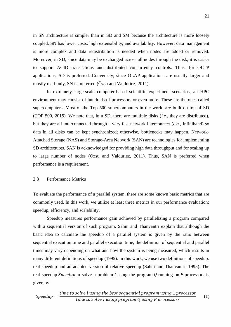
real speedup to solve a problem using the program running on processors is
given by
(1)

22
1
The time to solve using the best sequential program is also known as theoretical time. This
time may hide overheads and assumes a perfect case scenario, which may be utopic in most
situations, causing performance gains to be hidden. For this reason, instead of using this
theoretical time to calculate the real speedup, using a relative speedup seems fairer. The
relative speedup is given by (Sahni and Thanvantri, 1995):
(2)
However, in large-scale simulations, running the program on only one processor may not
be possible because it is not rare to have an executing taking days or weeks to run on a single
processor. Taking all this time to run may not be viable, because it means more costs
(especially if the HPC environment is a cloud-based service), more energy consumption, and
more time spent on queues on clusters that are shared with many users. For this reason, we
adapt the (2 and define the RelativeSpeedup* as:
(3)
where and is the smallest number of processors the program could run for the
evaluation. We use both and in our experimental
evaluation in Chapter 6.
In addition to speedup, efficiency is another popular metric used to evaluate parallel
systems. It measures the fraction of time for which a processor was efficiently employed
(Sahni and Thanvantri, 1995). The efficiency of the system is calculated by dividing the
speedup by the number of processors used to run. Since we used two different definitions
for speedup, we also use two different definitions for the efficiency. The real efficiency
is calculated based on the real speedup (1):
(4)
Analogously, the relative efficiency can be calculated based on the
relative speedup as in Equation (2).
Finally, to measure how the system behaves when we vary the problem size and the
number of processors, we use the metric. The ideal scalability is that the
execution time remains constant when we multiply the problem size by a factor of and
multiply the number of processors by .

23
Related Work 2.9
In previous sections, we argued that to support large-scale computer-based simulations, a
SWfMS needs to manage three types of data: execution data, provenance data, and domain
data, and we have defined the term provenance database to signify a data repository that
contains all of them, jointly. In introduction, we explained that some SWfMSs use a
distributed data control based on flat files and some of them use a centralized DBMS at
runtime to store one of the three types of data. We also argued that managing a provenance
database at runtime enables powerful advantages (Section 2.5). In this section, we are going to
mention existing parallel SWFMs in respect to their data management capabilities.
To the best of our knowledge, only Swift/T (Wozniak et al., 2013) and Pegasus
(Deelman et al., 2007) are acknowledged for running on large HPC environments. Swift/T is
a highly scalable parallel SWfMS that uses a distributed data management based on flat files
and stores provenance data in the end of the workflow execution. Thus, although it is good for
performance, its data analytical capabilities, including execution monitoring at runtime and
user steering, are limited. Pegasus stores execution data using a centralized DBMS and stores
provenance data in flat files, which are loaded into the database in the end of execution. Since
it uses a centralized DBMS, it suffers from a contention point. Moreover, since it does not
store the other two types of data at runtime, its analytical capabilities and interactive
execution are also limited.
For this reason, since SCC is the only existing SWfMS that manages a provenance
database (composed of the three types of data – Section 2.5) at runtime using a DBMS, it is
the only SWfMS that must be concerned about efficient mechanisms for capturing these data
at runtime to enable the mentioned advantages and to keep good efficiency. We highlight that
although SCC is directly related to this work, we do not mention it in this section. Instead, we
dedicate the next chapter for it (Chapter 3). Several previous works from our research group
have already surveyed with more details other existing SWfMS that enable provenance data
analyses (mostly in the end of workflow execution). Some of these works are reported by
Ogasawara (2011), Oliveira (2012), Dias (2013), and Silva (2014).

24
3 SCICUMULUS/C²
SciCumulus/C² (SCC) (Silva et al., 2014) is a parallel Scientific Workflow Management
System (SWfMS) developed by the High Performance Computing and Databases research
group4
at COPPE/Federal University of Rio de Janeiro and at Fluminense Federal University.
It is based on a collection of works from many researchers, undergraduate students, and
masters’ and PhD’s theses. Essentially, SCC was developed to benefit from the results of two
main initiatives: SciCumulus (Oliveira et al., 2010) and Chiron (Ogasawara et al., 2011;
Ogasawara et al., 2013). Chiron is a parallel workflow execution engine that takes advantage
of clusters and grids. SciCumulus utilizes the main characteristics and algorithms of Chiron
and adds special techniques to take advantages of cloud properties, such as elasticity, at
runtime (Oliveira, 2012). SCC aims at integrating Chiron and SciCumulus in order to propose
a more flexible parallel SWfMS that takes advantages of a wider variety of HPC
environments (Silva et al., 2014). To the best of our knowledge, they are the only current
parallel SWfMS that stores the three types of data jointly on the same Provenance Database
(Section 2.5). We use most of the core concepts introduced in Chiron, we keep the special
algorithms that take advantage of cloud environments introduced in SciCumulus, and use the
most recent version of SCC, which integrates them all, to serve as a basis for our work. For
this reason, the most important concepts of these systems that are for particular interest for
this dissertation are explained in this chapter.
SciWfA: a workflow algebra for scientific workflows 3.1
SCC manages a scientific workflow and the data that flows between each activity that
composes a workflow. We argue that scientific workflows in large-scale computer-based
experiments are data intensive, require HPC (as seen in Sections 2.1 and 2.2, and should not
miss relevant optimization opportunities, especially in parallel executions (Ogasawara et al.,
2011). To cope with this, Ogasawara et al. (2011) propose an algebraic approach that
facilitates complex dataflow definition, parallel data management of the data that flows
between activities, and enables optimizations of scientific workflow executions at runtime.
The Scientific Workflow Algebra (SciWfA) is an extension of the well-established relational
algebra, which is the basis for query processing and optimizations in relational database
systems (Özsu and Valduriez, 2011).
4 hpcdb.wordpress.com

25
In SciWfA (Ogasawara et al., 2011), each activity 𝑌 {𝑌} is associated to an
algebraic operator . Where {𝑌} is a set containing all activities in a determined workflow
and { }. Moreover, 𝑌 consumes a
set (or relation, as it is traditionally called in relational algebra) of input tuples and
produces a set of output tuples. The operator may also need an additional operand .
Hence, we may state that
𝑌 (5)
Additionally, the algebraic operator is defined depending on the ratio between the
number of tuples consumed and produced for a determined activity invocation, as we can see
in Table 1.
Operator Type of Operated
Activity Additional Operands
Ratio between
consumed and
produced tuples
Map Application Relation 1:1
SplitMap Application File Reference or Relation 1:m
Reduce Application Set of aggregating attributes or Relation n:1
Filter Application Relation 1:(0-1)
SRQuery Relational Algebra
Expression Relation n:m
MRQuery Relational Algebra
Expression Set of Relations n:m
Table 1 – SciWfA operations (adapted from Ogasawara et al., 2011)
The ratio between consumed and produced tuples is calculated based on the cardinality
(i.e., number of tuples) of the consumed input set and produced output set. This means that in
a workflow execution, a same application is invoked multiple times each of which consuming
a tuple (or set of tuples) and generating a tuple (or set of tuples) (recall from Section 2.3).
However, these applications that are invoked and managed by SCC are usually made by third
party companies or institutions that are not necessarily aware of SciWfA. As a consequence,
each invocation may not produce the necessary output tuples, which are very important for the
provenance gathering mechanism and to serve as input for the next linked activity. For this
reason, the SciWfA relies on the definition of an important concept called activation.
Activation and Dataflow strategies 3.2
According to Özsu and Valduriez (2011), an activation is “the smallest unit of sequential
processing that cannot be further partitioned”, i.e., cannot be further parallelized. In Chiron,

26
the core of SCC, an activation can be simplified as an activity invocation. Further, Ogasawara
et al. (2011) explain that it is a “self-contained object that holds all information needed to
execute a workflow activity at any core” on the HPC environment. That is, it contains which
application to invoke, which data to consume and what the schema of the data that will be
produced is.
Moreover, due to the reasons mentioned in Section 3.1, the concept of activation in
SCC is more than an activity invocation. It is necessary to define sub-concepts inside of it.
These are instrumentation, invocation, and extraction that altogether form an activation
(Ogasawara et al., 2011). Before the workflow execution, users define the data schema of the
input and output relations of all activities in the workflow. In instrumentation, input tuples
are extracted and the application invocation is prepared according to the defined input schema.
An invocation launches an application on a processor in the HPC environment, consuming the
input tuples defined in instrumentation and produces output tuples. Finally, in extraction,
produced output tuples are collected. Provenance data are gathered since the beginning until
conclusion of an activation. Typical gathered provenance data aids the scientists to answer, in
a high level of details, questions like: Is an activation still running? Has any error occurred? If
yes, which errors? How long did an activation take to completely execute? More importantly,
since different values for domain-specific parameters (e.g., speed of wave – seismic – or point
of the sky – astronomy) may impact of application performance or even may introduce
application errors, all those provenance data can be associated to domain-specific input and
output data. This enables rich analyses at runtime and execution monitoring (Oliveira et al.,
2014; Souza et al., 2015). The formal definition of an activation and its composing parts can
be found in (Ogasawara et al., 2011).
Regarding dataflow strategies, there are two in SCC: First Tuple First (FTF) and First
Activity First (FAF) (Ogasawara et al., 2011). To explain this, we use a simple workflow
example: two activities A1 and A2, being A2 dependent on A1. In FTF, an A2 activation only
waits until its necessary input tuples are produced by an A1 activation. This is a typical
pipeline dataflow. In contrast, in FAF, A2 only begins to execute when all A1 activations are
completely executed. In other words, A2 remains blocked until A1 finishes. We only used the
FAF strategy in our experiments as in almost all experiments executed in SCC (Chapter 6).

27
Centralized DBMS 3.3
SCC relies on a centralized DBMS to manage its Provenance Database. Although this brings
powerful advantages as mentioned in Section 2.5, this also leads to some drawbacks. We
highlight five disadvantages, especially comparing with the utilization of a DDBMS.
First, a centralized DBMS introduces a single point of failure in the parallel system.
That means that if the node that hosts the DBMS fails, the entire system fails. Second, if
compared with a DDBMS, it cannot handle a large dataset as efficiently as a DBMMS. Third,
it does not have special algorithms or techniques to take advantages of parallel execution on
multiple nodes in an HPC environment. Forth, a centralized DBMS is not as scalable as a
DDBMS. Finally, a DDBMS can handle a higher number of requests from clients than a
centralized DBMS. However, it is important to notice that despite the drawbacks, a
centralized DBMS uses less computing resources than a DDBMS, since only one node is
necessary whereas in a DDBMS, generally, the greater the data size, access rate, or
availability requirements, the more nodes are required to keep latency low and the system
available.
Architecture and Scheduling 3.4
SCC’s architecture is organized in a distributed fashion consisting of multiple nodes, which
we especially call SciCumulus Nodes (SCN). The core of SCC is instantiated on each SCN,
where the scientific workflow is effectively executed. The architecture is managed following
a master-slave policy. The master node manages the distribution of activations among all SCN.
Moreover, the master node is also an SCN node, which means that it also runs activations, but
it will not need to send MPI messages to get tasks, since tasks are just one hop away from the
database, and not two, like the other SCNs that are not masters. In addition to managing
activations distribution among all SCN, the master node is also responsible for storing data in
the Provenance Database. All slaves are connected to the master via a network interconnect
and all SCN access a shared disk. We note that there may be bottlenecks at the master node due
to a centralized management at a single site and due to the fact that the master node is the only
SCN enabled to access the provenance database. Furthermore, a database server is utilized to
host the DBMS that manages the Provenance Database. This architecture is illustrated in
Figure 5.

28
Figure 5 – SCC architecture
Regarding activations scheduling, SCC implements a CWQ BoT architecture and
tasks scheduling (recall from Section 2.4.1). Basically, master node is the only one that can
access the BoT (which is managed by a DBMS) to retrieve tasks and distribute them among
slaves. More specifically, it works as follows. The master node waits for requests from slaves.
A slave requests work and waits until the master sends an activation. Then, the master
accesses the database to retrieve the next activation that is ready to be executed. Following,
the master sends a massage containing the activation to the requesting node. The requesting
node receives the activation, executes it, and sends the master a feedback message containing
provenance data about the execution. Finally, the master receives the sent data, stores them in
the database, and waits for new requests. The execution finishes when all activations from all
activities are completely executed and provenance data of each individual execution is stored.
SCC is implemented in Java and utilizes MPJ5 (MPI for Java) for message passing among all
nodes in the cluster and Java built-in threads6 for concurrent programming in the shared-
memory architecture within each node.
Concerning software architecture, SCC is organized in four modules (Silva et al.,
2014). (i) SciCumulus Starter (SCStarter) – which facilitates workflow execution submission
on HPC environments. Common actions include automatic preparation of all machines that
5 http://mpj-express.org
6 http://docs.oracle.com/javase/tutorial/essential/concurrency/procthread.html

29
will be used during execution (e.g., VM instantiation in a cloud environment), conceptual
workflow insertion into the database, and instantiation of the workflow execution engine on
each machine; (ii) SciCumulus Setup (SCSetup) – which is used to insert, update or delete
conceptual workflows into or from the provenance database; (iii) SciCumulus Core (SCCore)
– which is the main module. It concretizes the conceptual workflow. It contains the main SCC
logic, including runtime optimizations based on the SciWfA (Ogasawara et al., 2011), fault
tolerance (Costa et al., 2012), intra-node parallelism taking advantage of shared-memory
architecture within each machine, adaptive execution (Oliveira et al., 2010), and so on. This is
the module that is effectively instantiated on each SCN; and finally (iv) SciCumulus Query
Processor (SCQP) – which aids users to submit SQL queries to the provenance database.
Although users can connect to the DBMS via other means (such as the ones provided by the
DBMS itself), this module simplifies the database connection so analytical queries can be
conveniently submitted to the provenance database by users. Queries results are returned to
users’ standard output, which can be redirected to semi-structured files (e.g., CSV) and
consumed by services that plot graphs to facilitate data visualization. These are the main
features, functionalities, and characteristics of the parallel WFMS we base this dissertation on.

30
4 BAG OF TASKS ARCHITECTURES SUPPORTED BY A DISTRIBUTED
DATABASE SYSTEM
In this chapter, we propose our main theoretical contribution. We propose two conceptual
distributed architectures for a BoT that relies on a Distributed Database Management System
(DDBMS). We define these architectures’ tasks scheduling, load balancing, fault tolerance,
and other issues. In Section 4.1, we propose a novel design of a BoT application. It is a high
level tasks distribution design and scheduling in a BoT application and does not depend on a
DBMS. However, it serves as inspiration and basis for our architectures that rely on a
DDBMS. In Section 4.2, we briefly introduce and explain the two architectures. In Section
4.3, we discuss common characteristics between them. In Section 4.4, we define the first
architecture and, in Section 4.5, the second.
Work Queue with Replication on multiple Masters 4.1
Before introducing our architectures proposal, we first propose a novel task distribution
design and scheduling of a BoT application. Although this does not depend on a DBMS, we
will show that it serves as an inspiration and basis for our actual architectures proposal.
We begin this proposal by enumerating advantages and disadvantages of two designs
studied in Section 2.4: Work Queue with Replication (Section 2.4.2) and Hierarchical Work
Queue (Section 2.4.3).
WQR advantages
i. It May achieve higher performance than the simple CWQ (Silva et al., 2003);
ii. Comparing with CWQ and HWQ, it has better use of data locality (Paranhos et
al., 2003; Anglano et al., 2006). In WQR, the necessary data is likely to be
locally stored, which does not occur in CWQ and HWQ;
iii. Higher availability than simple CWQ and HWQ because of the replicas;
iv. No task transmission between master and slaves;
v. Ability to accommodate large problems when partial replication is used.
WQR disadvantages
i. Communication bottleneck may occur due to centralization at the master node;
ii. If partial replication is used, choosing the victim node for work stealing needs
to be carefully evaluated because it may lead to communication overhead;
iii. If partial replication is used, there may exist tasks transmission (work stealing)
among slaves;
iv. Single point of failure at the central node.
HWQ advantages

31
i. Multiple masters lead to less congestion at a centralized node;
ii. If M and S are wisely chosen, congestion at the central node is avoided;
iii. HWQ may accommodate larger problems (Silva and Senger, 2011).
HWQ disadvantages
i. HWQ model does not take as much advantage of data locality as WQR;
ii. HWQ has single points of failure;
iii. There is task transmission in both levels of the hierarchy. That is, between
supervisor and masters and between masters and slaves.
iv. There is an added layer of bureaucracy between the slaves and the main owner
of the BoT. That is, compared with a one-level hierarchy (e.g., CWQ), more
communication is needed so a slave can reach a task;
v. To the best of our knowledge, there is not an optimal general method to find M
and S, even statically. As a result, the choice remains empirical;
vi. Computation load balancing is not clearly specified;
vii. Single point of failure at the central node.
Table 2 – A summary of the advantages and disadvantages of both WQR and HWQ.
Given these facts, we can combine characteristics of replication and hierarchy to
propose the Work Queue with Replication on multiple Masters (WQRM). In WQRM (Figure
6), there are M masters and σ slaves in the cluster. The number σ of slaves in the whole cluster
is given by the sum of all slaves in all clusters ci. That is:
σ ∑ (2)
Figure 6 – Work Queue with Replication on Masters design.

32
Like in WQR, the supervisor does not own the bag of tasks. Instead, the BoT is
replicated in all masters. This increases availability because if a master fails, another master
may own the failing portion of the BoT and the supervisor coordinates the failure recovery.
Identically to WQR, between master nodes and the supervisor there are only scheduling
messages, i.e., no task transmission. Each cluster ci works exactly like the CWQ, that is, there
is task transmission between a master and slaves. Just like in WQR with partial replication,
when one master node ends its portion of the work queue and becomes idle, the supervisor
helps calculating whether or not it is advantageous to ask the idle master to steal tasks from a
victim busy master.
Regarding availability, failure recovery strategies may be applied in the slave nodes by
taking advantage of replication (Anglano et al., 2006). In addition, to provide higher
availability, the secondary supervisor’s role is just to eliminate a single point of failure. That
is, if the main supervisor fails, the secondary supervisor takes its place.
Regarding advantages and disadvantages in WQRM:
a) From WQR, in respect to the advantages, WQRM inherits most of them. Only the
advantage (iv) is not fully given because even though there is no task transmission
between supervisor and masters, there is between masters and slaves. In respect to
the disadvantages, all of them are inherited. However, since there are many
masters, contention in a single centralized point is less likely to occur, like in the
hierarchical model.
b) From HWQ, the only inherited characteristic is having multiple masters, which is
its greatest advantage. For his reason, in respect to the advantages, WQRM inherits
all of them. In respect to the disadvantages, (i) still remains because WQRM only
takes advantage of data locality between masters and the supervisor (just like
slaves and master in WQR). This is useful for work stealing among masters, but
not useful for scheduling tasks among slaves. Moreover, disadvantage (v) is still an
open problem. All other disadvantages are canceled because of replication,
addition of a second supervisor, and work stealing among masters.
By proposing WQRM, we want to add an extra option to the existing BoT designs
(Section 2.4) so that we can choose among them which we will use as inspiration and basis
for our architecture that relies on a DDBMS, which will be responsible to hold the BoT. It is
important to avoid communication bottleneck due to centralization, which motivates us to
choose a design with multiple masters (managers of the BoT). Especially, a design based on
replications has many advantages that we are very interested in. For this reason, we decide to

33
choose WQRM, which combines advantages of replication and hierarchy (specifically,
multiple masters). Therefore, among the four tasks distribution designs previously presented
(CWQ, HWQ, WQR, and WQRM), we choose WQRM so our architecture supported by a
database system will be based on. In next section, we discuss two architecture alternatives and
explain which one we choose to implement our solution.
Brief introduction to Architectures I and II 4.2
Most BoT implementations found in literature do not utilize a database system (Silva et al.,
2003; Anglano et al., 2006; Silva and Senger, 2011). For this reason, we need to highlight
three important motivations for using a DBMS, a distributed DBMS in special, in a BoT
problem.
The primary motivation for using a DBMS in our architecture (in a SWfMS context) is
that in a workflow execution, lots of data are continuously managed in a fine grained level as
data are processed all over the dataflow. Thus, by using a DBMS, it is possible to query
complex experiments’ execution logs, perform advanced data analyses, as well as enable
humans to interact with the remaining tasks to be executed through updates on the database,
everything during runtime, as we have argued in Section 2.5. We do not want to abdicate
these powerful advantages.
The secondary, but also very important, motivation for using a database system is that
most DBMSs implement very efficient mechanisms that are essential in a HPC scenario. For
example, any DBMS implements efficient concurrency control mechanisms. Especially, most
relational DBMS (including the centralized ones) implement well-known algorithms and
strategies to guarantee atomicity, consistency, isolation, and durability in transactions.
Moreover, distributed database systems enable robust parallel access and storage of data,
usually in larger sizes than regular centralized DBMS. Further, sharding, i.e., partitioning the
database into multiple nodes is also well-studied and implemented in many distributed
DBMSs. Besides, failure recovery is also an important functionality in a DDBMS.
Furthermore, efficient utilization of cache memory is also a common feature in DBMSs,
including centralized ones (Özsu and Valduriez, 2011). Additionally, a DBMS (either
centralized or distributed) may be implemented to run completely in-memory instead of
performing I/O operations to disk, which would enhance performance. Therefore, having a
DBMS – which already implement most of these mechanisms usually very efficiently – to
take care of all these complex issues, will alleviate the effort on developing such complex

34
controls in a given parallel application. In this way, the developers would focus on specific
concerns that are related to specific uses of the application, instead of having to worry about
implementing tasks scheduling and dealing with complex concurrency issues. In our case, we
want to focus on controlling the parallel execution of workflows and store important data in
the provenance database.
The tertiary motivation specifically relies on a distributed database system. In addition
to the above arguments regarding the utilization of a distributed database system, there is still
the fact that, by using one, we can take more advantage of the parallel hardware architecture,
which is common in HPC environments. Furthermore, a centralized database system will
likely suffer from congestion in a scenario with many processing nodes. For these reasons, a
distributed database system is more convenient in an HPC scenario.
In next sections, we describe two architectures, based on WQRM design, supported by
a distributed database system: Architecture I, which uses WQRM by making an analogy
between masters and data nodes; and Architecture II, which has many similarities with
Architecture I, but has different number of partitions and data nodes.
Common Characteristics 4.3
Similarities and differences between Architectures I and II are in respect to the work queue. In
common, the work queue is managed by a distributed database system and it is fully
partitioned, that is, horizontally fragmented across all nodes in the cluster of database nodes.
This significantly increases parallelism (Özsu and Valduriez, 2011). Moreover, regarding
availability, both architectures share the same characteristics inherited from WQRM design.
Yet, if a node hosting a work queue partition fails, there is still at least an extra replica that
may be utilized.
Although inspired by WQRM and many analogies will be made to explain both
architectures, WQRM and the architectures are not exactly one-to-one analogous. The
architectures do not explicitly have multiple master nodes functioning as schedulers. We may,
rather, establish the DDBMS (as a whole) as a great “centralized” scheduler, which implies a
similar behavior to CWQ.
Nonetheless, instead of having slaves requesting tasks to a master through regular
message passing, like in common CWQ implementations, we have slaves sending structured
queries to a distributed database system. Instead of having a master to receive the slave

35
request, get the next ready task and send it to the slave, we have the DDBMS to play the very
same role.
In spite of the fact that the message passing primitives (e.g. send and receive) are
basically the same in either implementations (common CWQ implementation or DBMS
supported implementation); and that data transfer happens in a similar way, the main
advantage is that we rely the scheduling on a third party system. That is, we apply the idea of
outsourcing. More importantly, this third party system we rely on is known to be specialized
in concurrency control mechanisms (Özsu and Valduriez, 2011). Furthermore, all benefits we
pointed out in our secondary motivation in the beginning of this section are applicable. Thus,
we count on a trusted and highly specialized third party system to alleviate our work so we
can spend more efforts on the actual application.
Despite noting a CWQ behavior resemblance, we emphasize that a DDBMS is utilized
instead of a single central node, as it is in CWQ. In other words, there is not a centralized
single master at all. A DDBMS is composed of many data nodes which diminishes the
centralization problem that causes congestion in CWQ. We use the term data node (dn) to
signify a node that hosts the process that manages partitions of the database. A data node also
contains data of the DDBMS. In other words, a data node owns and manages part of the bag
of tasks. This also resembles the fact that multiple master nodes hold BoTs in the WQRM
design.
It is important to highlight that since we are relying on a database solution, a new role
takes place in the scenario: the database server, which we shorten as dbs. Database servers
just listen to connections and applications commonly connect to the database through
connection drivers (e.g., JDBC or ODBC7). Even though the dbs are usually just responsible
for listening to connections, they may play an important role regarding communication load
balance. Some distributed DBMSs implement mechanisms to improve communication load
balance so contention at the database may be avoided, which is very valuable for us. However,
the presence of a new role introduces a new problem that we need to deal with because of the
database utilization. There is a need to determine a good number of dbs in the cluster, which
may also be empirical. We denote this number by q.
Furthermore, an initial connection distribution is needed. That is, each slave needs to
know in advance which dbs it will connect to. A supervisor node needs to take care of this.
Plus, it is important to even up communication load across the q dbs. Otherwise, there may be
7 http://en.wikipedia.org/wiki/Java_Database_Connectivity and
http://en.wikipedia.org/wiki/Open_Database_Connectivity

36
a dbs with a heavy load of slaves connecting to it while there are others lightly loaded. This
communication load balance may be easily achieved by making use of a circular distribution
policy, as we show in the algorithm proposed in Section 4.4.4. Next, we describe both
architectures in details.
Architecture I: Analogy between masters and data nodes 4.4
Just like there are M masters in WQRM, there are M data nodes in Architecture I (Figure 7).
In next sections we will explain the scheduling process, which consists of slaves querying the
data nodes in order to retrieve tasks (analogous to slaves asking masters for work).
Figure 7 – Architecture I: Master nodes are data nodes
Furthermore, to increase availability in the system, each slave Sij may connect and
query the database cluster via two different dbs nodes: the main dbs node connection,
represented by dashed lines in Figure 7 and the secondary dbs node connection, represented
by dotted lines. If one dbs fails, all slaves that were connected to it just need to connect to
their secondary dbs.
4.4.1 Parallel data placement
Regarding parallel data placement in the database system (recall from Section 2.6.3), the
whole work queue is horizontally fragmented into M (number of data nodes in the cluster)

37
partitions. Each partition ρi is responsibility of and physically stored in dni and replicated
elsewhere. Each partition ρi initially contains T = ceiling(Ttotal/M) tasks, where Ttotal is the
total number of tasks in the BoT. To place T tasks in each partition, a hash function on the
data node id may be applied.
4.4.2 Task distribution and scheduling
This is how initial task distribution happens in this architecture. Initially, given that there are
M data nodes, the supervisor is responsible for assigning each task to a data node in a circular
fashion. This is done inserting tasks in the work queue relation in the database assigning the
data node id to the task and the hash function mentioned previously (Section 4.4.2) will take
care of placing the task in the right data node. Similarly, the supervisor also assigns a data
node to each slave node so that each slave will know which data node will be queried.
It is worth noting that only in close-to-homogeneous problems (that is, all tasks cost
approximately the same), the static initial distribution will provide near to optimal load
balance. In heterogeneous problems, though, this initial distribution needs to be dynamically
“corrected” during runtime. However, even in homogeneous problems, load imbalance may
still occur in very long running executions. Thus, work stealing and more sophisticated load
balancing may still be needed.
After all initial task distribution and data placement, the actual scheduling begins and
it works similarly to what we described for the CWQ (recall from Section 2.4.1). A slave
sends a query to retrieve tasks from its partition which is physically stored in dni and
replicated elsewhere. The DDBMS is responsible for an efficient concurrent management
from the multiple requests and then it delivers the right tasks to the requesting slave. The
requesting slave becomes busy while executing its tasks. When a slave finishes its work load,
it stores the results in the provenance database. Then, it becomes idle and ready to retrieve
more tasks from the database. This is done until all tasks in the bag of tasks are completed.
4.4.3 Load balancing
Load balancing happens analogously as specified in WQRM. When all tasks in a data node
are completed, a slave notifies the supervisor of the situation. Then, the supervisor calculates
whether or not work stealing is advantageous. If it is, a victim data node must be selected. If
we use the heuristic of choosing the most loaded data node, we just need to query the database

38
to easily get this information. Finally, after selecting the victim, say dnj, the supervisor needs
to move data from the partition ρj to partition ρi.
4.4.4 Algorithm for distributing dbs to achieve better communication load balance
In our architectures, slaves access the distributed database via connection to the dbs nodes. In
other words, the dbs are the only nodes that the slaves are aware of to get access to data in the
distributed database. A common scenario is when the number of slaves is much greater than
dbs nodes and communication load imbalance may occur. If, for example, there are 20 slaves
and only 2 dbs nodes, (say dbs1 and dbs2) there would be communication load imbalance if
19 slaves connect to dbs1 e only one slave connects to dbs2. For this reason, we need extra
functionalities to improve communication load balance. To tackle this, we also propose our
own algorithm for distributing dbs nodes to all slaves in a balanced way. In our previous
example, one balanced way to distribute dbs nodes would be 10 slaves connecting to the
DDBMS via dbs1 and the other 10 connecting via dbs2. Moreover, we also need to assign a
secondary dbs 2 for each slave to increase availability in case the primary dbs fails. In other
words, each slave has a primary dbs through which it connects to the DDBMS and a
secondary dbs that is used if the primary dbs fails.
The algorithm is divided into three parts. In part (i), if a physical machine is both slave
and database server, then, this slave machine connects to the distributed database through the
database server that is hosted on this machine. In other words, if a machine is both slave and
dbs, it assigns itself as the dbs. In part (ii), each slave assigns a dbs to it in a circular fashion.
Each dbs can serve at most W/q, where W is the number of remaining slaves to be assigned
and q is the number of dbs nodes. In part (iii), each of the W remaining slaves is assigned to a
dbs, also in a circular fashion. This algorithm is formalized as shown in Figure 8. In addition
to this algorithm, we discuss in Section 5.3 that in our implementation, we may also make use
of features provided by the DDBMS to improve communication load balance.

39
Figure 8 - Algorithm for dbs distribution to slaves
Algorithm 1: Distributing database servers to slaves
Input:
Ldbs: List of database server machines
Lw: List of slave machines
Output:
-
1.
2.
3.
4.
5.
6.
7.
8.
9.
10.
11.
12.
13.
14.
15.
16.
17.
18.
19.
20.
21.
22.
23.
24.
25.
26.
27.
28.
29.
30.
31.
32.
33.
34.
35.
36.
37.
38.
39.
40.
41.
42.
43.
44.
45.
46.
47.
48.
49.
50.
function distributeDatabaseServers(Ldbs, Lw)
int circular 0
int i 0
int quotient 0
int primDBindex 0
int secDBindex 0
// Part (i)
for each machine in Ldbs do
if exists machine in Lw then
machine.mainDBS machine
circular circular + 1 remove(machine, Lw)
end if
end do
quotient |Lw| div |Ldbs|
// Part (ii)
while i < |Lw| do
primDBindex circular mod |Ldbs|
Lw[i].mainDBS Ldbs[primDBindex] if |Ldbs| >= 2 then
secDBindex abs ( ( |Ldbs| 1 circular ) mod |Ldbs| )
Lw[i].secondaryDBS Ldbs[secDBindex] end if
i i + 1 if quotient = 0 then
circular circular + 1 exit while
end if
if i mod quotient = 0 then
circular circular + 1 end if
end do
// Part (iii)
while i < |Lcn| do
primDBindex circular mod |Ldbs|
Lw[i].mainDBS Ldbs[primDBindex] if |Ldbs| >= 2 then
secDBindex abs ( ( |Ldbs| 1 circular ) mod |Ldbs| )
Lw[i].secondaryDBS Ldbs[secDBindex] end if
i i + 1
circular circular + 1 end do
end function

40
4.4.5 Advantages and disadvantages
Advantages of using Architecture I are: (i) Assuming that M is wisely chosen (recall from
Section 4.1) as well as q is good enough, there will be less congestion at the database and
parallel query execution may be well explored; (ii) due to utilization of secondary nodes (for
master node and for db server nodes) and due to reasons inherited by basing on WQRM, this
architecture is able to provide high availability; and (iii) this architecture provides great
flexibility for adding slaves, even dynamically during runtime. Everything a slave needs to do
to join the executing team is to connect to the DBMS through any dbs. Despite being likely
unnecessary, a more sophisticated strategy to choose the least loaded dbs may be
accommodated to preserve communication load balancing. Then, after connecting, the
recently joined slave can start executing by following the scheduling policy described
previously. Removing slaves is similar to the slave failure recovery process as discussed in
the beginning of this section.
The disadvantages of Architecture I are related to scalability problems, which are
likely to occur in a scenario with a large M because it will be harder for the DBMS to manage
a large number of data nodes. A large number of data nodes means that data will be spread
throughout many actual machines. Many distributed DBMSs do not scale data nodes up to a
really big number, say hundreds of nodes. In addition, the more partitions, the more it will be
taken advantage of parallel executions. However, requiring that each partition needs to be
physically stored in each data node implies that many data nodes will be needed in order to
achieve greater parallelism. This, as mentioned, may also lead to a scalability problem. Since
we want our architecture to be adaptable to a large environment, this is a critical limitation.
Architecture II: Different number of partitions and data nodes 4.5
Architecture II (Figure 9) functions mostly like Architecture I. The main difference is that in
Architecture II, we do not force each partition ρi to be physically stored in dni. This implies
that the number of partitions does not need to be equal to the number of data nodes. Rather,
the cluster of database nodes is composed of d data nodes and the work queue is partitioned
into M partitions.

41
Figure 9 – Architecture II: Analogy between masters and partitions of the work queue
This introduces much more flexibility than in Architecture I, since we may have a
greater number of partitions than of physical data nodes. As said previously, more partitions
lead to better parallelism. Multiple data nodes are more costly than multiple partitions.
Although more flexibility and generality are given to Architecture II, it introduces one
new problem: choosing d. Table 3 summarizes which parameters need to be adjusted in order
to achieve good performance.
Parameter Meaning
d Number of data nodes in the database cluster
q Number of dbs nodes
M Number of partitions of the work queue
S
Number of slaves that connect to a dbs node. If q is known, this
may be simplified as S σ / q. Recall from Section 4.1 that σ is
the total number of slaves on the HPC environment.
Table 3 – Parameters that need to be adjusted
In spite of seeming very complex to define all these parameters, a simplification of the
problem is presented in Section 5.5.

42
4.5.1 Parallel data placement
Regarding parallel data placement in the database, the work queue is fully partitioned (Özsu
and Valduriez, 2011) into M horizontal fragments, or partitions, across all data nodes. Each
partition ρi initially contains T = ceiling(Ttotal/M) tasks, where Ttotal is the total number of
tasks in the BoT. To place T tasks in each partition, a hash function on the partition id may be
applied, as in Architecture I.
It is important to highlight that M may be very large in a large-scale scenario.
Although it is harder to manage by the DDBMS, this will significantly improve parallelism.
Especially, this may cause so much improvement in parallelism that congestion at the DBMS
might be highly alleviated. However, it needs to be carefully evaluated (e.g., testing speedup
and scalability) to investigate if no overhead will occur.
4.5.2 Task distribution and scheduling
Initial task distribution happens in an analogous way to Architecture I. Initially, given that the
work queue is partitioned into M partitions, the supervisor is responsible for assigning each
task to partition in a circular fashion. This is done inserting tasks in the work queue relation in
the database assigning a partition id to the task and the hash function mentioned above will
take care of placing the task in the right partition. Similarly, the supervisor also assigns a
partition id to each slave node so that each slave will know which partition will be queried.
Load balancing also works similarly to Architecture I. The algorithm proposed for
improving communication load balance (Section 4.4.4) is also applied in Architecture II.
4.5.3 Advantages and disadvantages
Finally, the advantages of using Architecture II are the same of Architecture I. In addition,
Architecture II is more flexible since it does not require a large number of data nodes (e.g.
hundreds) to achieve enhanced parallelism. Moreover, Architecture II does not require that
the number of data nodes to be equal to the number of slave nodes, removing the main
disadvantage of Architecture I. However, Architecture II introduces more complexity since a
new parameter needs to be adjusted. This is explored in our experimental evaluation (Chapter
6).

43
In this section, we proposed two architectures supported by a distributed database
system. We described their main ideas, how they would work and discussed the benefits and
losses of using each of them. We chose to use Architecture II to implement because it has all
advantages of Architecture I and is more flexible. In the next section, we describe how we
implemented Architecture II.

44
5 SCICUMULUS/C² ON A DISTRIBUTED DATABASE SYSTEM
In this chapter, we explain details of the implementation of SciCumulus/C² on a Distributed
Database System (d-SCC). In Section 5.1, we explain how we chose the DDBMS technology
we used. In Section 5.2, we present MySQL Cluster. In Section 5.3, we present the
architecture of d-SCC, which is the Architecture II, presented in the previous section, fitting
MySQL Cluster’s architecture. In Section 5.4, we show an extra module we developed to
manage DDBMS issues. In Section 5.5, we describe parallel data placement and
fragmentation in our solution. In Section 5.6, we explain how we implemented tasks
scheduling and why we removed MPI for this. Finally, In Section 5.7, we discuss fault
tolerance and load balancing.
Technology choice 5.1
In order to accommodate either Architecture I or II, presented in the previous section, we need
a DDBMS technology. For this reason, we list necessary and desirable requirements.
First, the necessary requirements are: (i) It needs to provide efficient parallel and
distributed strategies (parallel query optimization and distributed concurrency control
mechanisms); (ii) It needs to be highly scalable – both (i) and (ii) are required because of the
distributed DBMS features that Architecture II relies on; and (iii) It has to be optimized for
OLTP queries – because multiple short and simple queries based on indexes are very
frequently performed in order to retrieve next runnable tasks and to update their status and
execution time when they finish.
Second, the desired requirements are: (i) It would be better if it were free licensed –
because we do not want to close our solution to a very specific DBMS technology; (ii)
SQL/relational model – SQL queries on a relational database with good indexes are known to
be efficient for quick and simple lookups, which are very frequent because of the scheduling
we described in Chapter 4, hence SQL queries would be desirable; (iii) it should implement
strong consistency – because besides retrieving tasks, slaves need to store back results of their
executions in the database. Thus, many updates occur at runtime and taking advantage of
strong consistency provided by the DBMS is desirable to facilitate our work; and (iv) it
should be able to be executed in shared disk architecture – because our motivating problem is
mainly focused on complex scientific applications, which are usually executed in very large
clusters operating on shared disk architecture Section 2.7)

45
Given these facts, we build up the following table.
Technology Relational/SQL Architecture License Main
Disadvantage
NuoDB NewSQL SN Very limited free
version License
VoltDB NewSQL SN Proprietary License
MemSQL NewSQL SN Free trial License
SparkSQL SQL SN Proprietary Little support
for OLTP
MySQL Cluster SQL SN Open No support
for SD
Oracle TimesTen SQL Both Proprietary License
Oracle Coherence KeyValue Both Proprietary License and
NoSQL
MongoDB Document SN Open NoSQL
Impala SQL-like SN Open
SN and
OLAP
optimized
HBase Column SN Open
SN and little
support for
OLTP
Presto SQL-like SN Open
SN and little
support for
OLTP
MonetDB Column SN Open
SN and
OLAP
optimized
Table 4 – DBMS technologies comparison
In Table 4, we mainly compare the technologies according to our needs previously
listed. All of them are said to be scalable and work on a distributed environment, with
distribution features. We first eliminate all options that provide little support for OLTP or are
mainly optimized for OLAP (online analytical processing), since we are mainly interested in
fast transactions rather than heavy analyses during execution. Proprietary technologies are
highly discouraged because of the reasons we stated; hence we cross out all DBMS
technology with a proprietary disadvantage. This leaves us to choose between MySQL
Cluster and MongoDB.
MongoDB is a NoSQL database, document-oriented. In addition to the desired
requirement (ii) previously mentioned, the SWfMS we are basing our implementation on
utilizes a data model that is essentially relational: PROV-Wf (Costa et al., 2013), as
presented in Section 2.5. Because of this, there are many relational queries that are executed

46
at runtime needed by the execution engine, which is totally based on the provenance database.
These queries generally involve both reads and writes, and joins among different relations.
NoSQL DBMS are not as concerned about ACID transactions as relational databases are,
which commonly implement strong consistent models. We need to keep all those writes
consistent, and these kinds of relational queries, involving joins, are better performed by
relational DBMS. Finally, one other important aspect is regarding development. Since SCC
already relies on a relational DBMS and the entire execution is driven by SQL queries, using
a different query language would require much more effort. By using a different DBMS, but
still a relational one, we could save lots of effort by just adjusting small differences in
specificities of the SQL dialect of this different relational DBMS.
MySQL Cluster is a relational DBMS, OLTP optimized, efficient for fast lookups,
provides efficient concurrency control mechanisms, and claims to provide high availability8
(Oracle, 2015a). Just like most conventional DBMS, it is also possible to execute OLAP
queries on MySQL Cluster. Additionally, its fault tolerance mechanisms make it a good
choice for removing a single point of failure introduced by using a centralized DBMS.
Besides, it is an in-memory database cluster and it tends to be faster than regular on-disk
DBMS. However, MySQL Cluster has a limitation for our needs. It does not support shared
disk architecture9. Anyhow, especially because of our limited choices, we gave it a try.
MySQL Cluster 5.2
MySQL Cluster requires three types of database nodes (or roles, as we call): ndbd, mysqld
and ndb_mgmd, which is a necessary manager node for MySQL cluster’s architecture. The
documentation recommends that each of these roles is placed on different physical machines
for higher availability purposes (Oracle 2015a). In Figure 10, it is shown MySQL Cluster
architecture and how its main components (i.e., the roles) communicate to each other. The
main role is the ndbd which is responsible for distributing queries, transaction management,
and data management. That is, most of the database processing is responsibility of the ndbd
role. Mysqld role basically works as a port through which clients or APIs may connect using
connection drivers (e.g., JDBC or ODBC) and issue SQL queries. Ndb_mgmd manages the
8 www.mysql.com/products/cluster
9 http://dev.mysql.com/doc/refman/5.1/en/mysql-cluster-overview.html
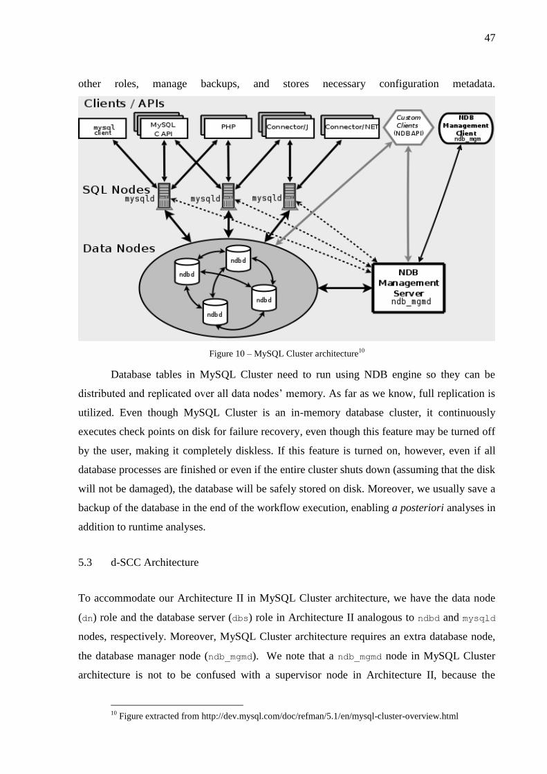
47
other roles, manage backups, and stores necessary configuration metadata.
Figure 10 – MySQL Cluster architecture10
Database tables in MySQL Cluster need to run using NDB engine so they can be
distributed and replicated over all data nodes’ memory. As far as we know, full replication is
utilized. Even though MySQL Cluster is an in-memory database cluster, it continuously
executes check points on disk for failure recovery, even though this feature may be turned off
by the user, making it completely diskless. If this feature is turned on, however, even if all
database processes are finished or even if the entire cluster shuts down (assuming that the disk
will not be damaged), the database will be safely stored on disk. Moreover, we usually save a
backup of the database in the end of the workflow execution, enabling a posteriori analyses in
addition to runtime analyses.
d-SCC Architecture 5.3
To accommodate our Architecture II in MySQL Cluster architecture, we have the data node
(dn) role and the database server (dbs) role in Architecture II analogous to ndbd and mysqld
nodes, respectively. Moreover, MySQL Cluster architecture requires an extra database node,
the database manager node (ndb_mgmd). We note that a ndb_mgmd node in MySQL Cluster
architecture is not to be confused with a supervisor node in Architecture II, because the
10
Figure extracted from http://dev.mysql.com/doc/refman/5.1/en/mysql-cluster-overview.html
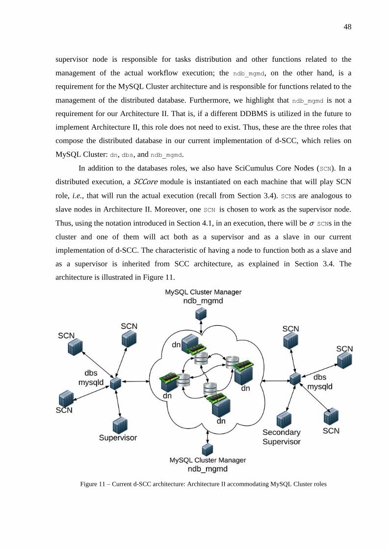
48
supervisor node is responsible for tasks distribution and other functions related to the
management of the actual workflow execution; the ndb_mgmd, on the other hand, is a
requirement for the MySQL Cluster architecture and is responsible for functions related to the
management of the distributed database. Furthermore, we highlight that ndb_mgmd is not a
requirement for our Architecture II. That is, if a different DDBMS is utilized in the future to
implement Architecture II, this role does not need to exist. Thus, these are the three roles that
compose the distributed database in our current implementation of d-SCC, which relies on
MySQL Cluster: dn, dbs, and ndb_mgmd.
In addition to the databases roles, we also have SciCumulus Core Nodes (SCN). In a
distributed execution, a SCCore module is instantiated on each machine that will play SCN
role, i.e., that will run the actual execution (recall from Section 3.4). SCNs are analogous to
slave nodes in Architecture II. Moreover, one SCN is chosen to work as the supervisor node.
Thus, using the notation introduced in Section 4.1, in an execution, there will be σ SCNs in the
cluster and one of them will act both as a supervisor and as a slave in our current
implementation of d-SCC. The characteristic of having a node to function both as a slave and
as a supervisor is inherited from SCC architecture, as explained in Section 3.4. The
architecture is illustrated in Figure 11.
Figure 11 – Current d-SCC architecture: Architecture II accommodating MySQL Cluster roles

49
Furthermore, in d-SCC, the BoT is completely placed in a distributed table and we
make use of MySQL Cluster features to improve communication load balancing11
, in addition
to the algorithm presented in Section 4.4.4. We give more details on how we distribute it
across all data nodes in Section 5.5
SciCumulus Database Manager module 5.4
As introduced in Section 3.4, SCC software architecture is built upon four modules:
SCStarter, SCSetup, SCCore, and SCQP. To conveniently manage the distributed database in
our solution, we developed an extra module: SciCumulus Database Manager (SCDBM). In
this section, we explain in details our added SCDBM module and modifications we needed to
adapt.
5.4.1 Pre-installation Configuration
In d-SCC, just like its predecessors, a list of machines on the HPC environment that will be
used in the workflow execution needs to be provided. The list is historically saved on a file
called machines.conf (Figure 12). These machines will compose the architecture and each
of them will play one or more roles (SCN, dn, dbs, ndb_mgmd) defined in Section 5.3.
11
http://dev.mysql.com/doc/refman/5.1/en/mysql-cluster-basics.html
# Number of processes
10
# Protocol switch limit
131072
# Entry in the form of hostname@port@rank
node1@20919@0
node2@20919@1
node3@20919@2
node4@20919@3
node5@20919@4
node6@20919@5
node7@20919@6
node8@20919@7
node9@20919@8
node10@20919@9
Figure 12 – machines.conf file example containing 10 machines

50
Configuring which role each machine will play may impact on performance, as we
explain and show in our experimental evaluation in Chapter 6. For this reason, in d-SCC, one
important configuration file, which we call installation.properties, is needed so users
can vary the architecture according to their needs. For example, a tradeoff between
performance and available resources needs to be analyzed, since the best performance may
demand a lot of computing resources. In installation.properties, users define values for
the parameters described in Table 3 from Section 4.5.1. More specifically, users need to
define three parameters: d (= number of dn), q (= number of dbs), and the number of
management nodes (ndb_mgmd).
After defining these three values, next step is to define which roles the machines may
accumulate. That is, to save resources, one may want each machine to play more than one role.
We divide this role accumulation concept into two types of accumulation: SCN and database
nodes.
For SCN accumulation, users define which database roles (i.e., dn, dbs, and ndb_mgmd)
a SCCore instance will play together with. For example, suppose we have 10 machines
available and we want all of them to play SCN role (i.e., to actually execute the workflow).
However, we need at least 3 roles for the database (dn, dbs, and ndb_mgmd). In this scenario
(10 SCN, 1 dn, 1 dbs, and 1 ndb_mgmd), we need to indicate that we want machines that will
play SCN role will also play dn, dbs, and ndb_mgmd. This means that three machines will play
two roles concurrently. On the one hand, this saves resources and more SCCore instances can
run hence more parallel execution; on the other hand, in three machines at least two processes
will compete for resources (especially memory and processor), which may interfere in
performance, as we discuss in our experimental evaluation (Chapter 6). Obviously, users are
able to indicate that each SCCore instance will run dedicatedly, i.e., machines that play SCN
role are not going to play database role.
For database nodes accumulation, users may want to indicate that a machine that plays
one of the database roles (dn, dbs, and ndb_mgmd) may accumulate more database roles. In
our exemplary scenario (10 SCN, 1 dn, 1 dbs, and 1 ndb_mgmd), we may want dbs and
ndb_mgmd roles to be played by the same machine, consequently the dn role will be played
dedicatedly by a different machine. We may combine both accumulation types to indicate
which of the four roles will be dedicated or will be concurrently played within a machine.
This brings flexibility to build the architecture according to the users’ interest. We vary the
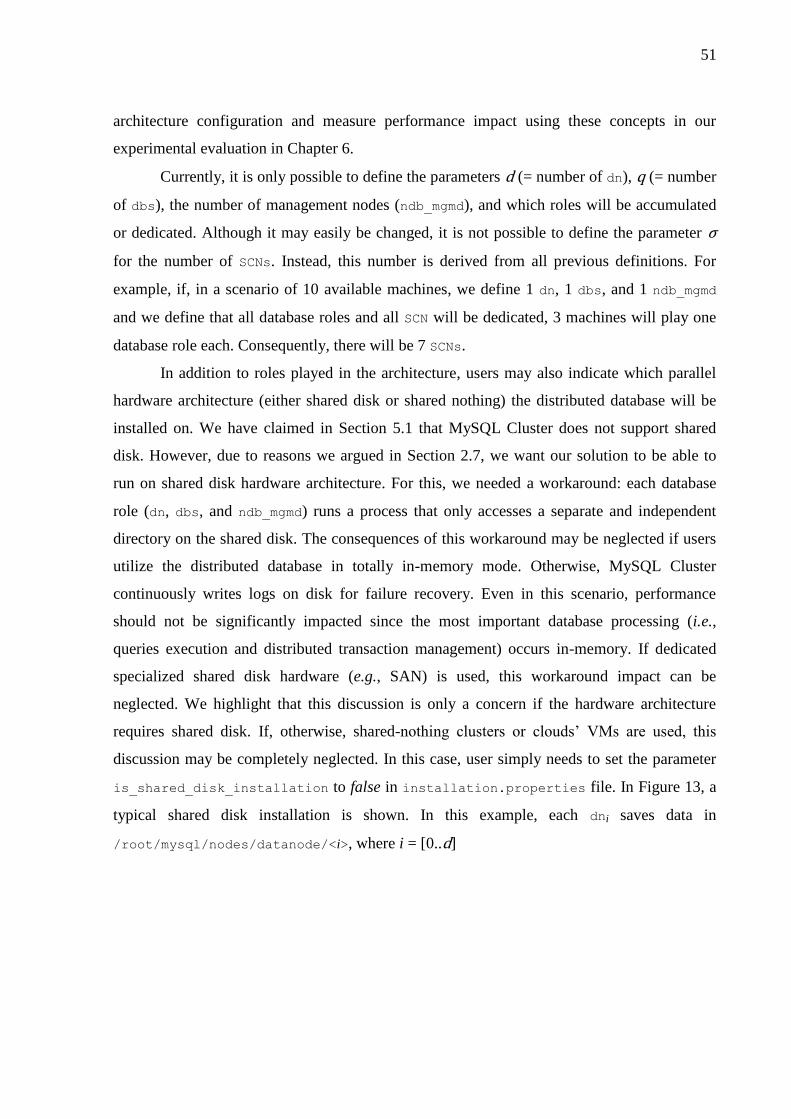
51
architecture configuration and measure performance impact using these concepts in our
experimental evaluation in Chapter 6.
Currently, it is only possible to define the parameters d (= number of dn), q (= number
of dbs), the number of management nodes (ndb_mgmd), and which roles will be accumulated
or dedicated. Although it may easily be changed, it is not possible to define the parameter σ
for the number of SCNs. Instead, this number is derived from all previous definitions. For
example, if, in a scenario of 10 available machines, we define 1 dn, 1 dbs, and 1 ndb_mgmd
and we define that all database roles and all SCN will be dedicated, 3 machines will play one
database role each. Consequently, there will be 7 SCNs.
In addition to roles played in the architecture, users may also indicate which parallel
hardware architecture (either shared disk or shared nothing) the distributed database will be
installed on. We have claimed in Section 5.1 that MySQL Cluster does not support shared
disk. However, due to reasons we argued in Section 2.7, we want our solution to be able to
run on shared disk hardware architecture. For this, we needed a workaround: each database
role (dn, dbs, and ndb_mgmd) runs a process that only accesses a separate and independent
directory on the shared disk. The consequences of this workaround may be neglected if users
utilize the distributed database in totally in-memory mode. Otherwise, MySQL Cluster
continuously writes logs on disk for failure recovery. Even in this scenario, performance
should not be significantly impacted since the most important database processing (i.e.,
queries execution and distributed transaction management) occurs in-memory. If dedicated
specialized shared disk hardware (e.g., SAN) is used, this workaround impact can be
neglected. We highlight that this discussion is only a concern if the hardware architecture
requires shared disk. If, otherwise, shared-nothing clusters or clouds’ VMs are used, this
discussion may be completely neglected. In this case, user simply needs to set the parameter
is_shared_disk_installation to false in installation.properties file. In Figure 13, a
typical shared disk installation is shown. In this example, each dni saves data in
/root/mysql/nodes/datanode/<i>, where i = [0..d]

52
Figure 13 – Example of a directory tree in a shared disk installation
One other important file that users need to be concerned about is MySQL Cluster’s
initial configuration file (config.ini), which is used to define many important configuration
parameters12
. Currently, we specifically determine values for the following parameters (Table
5).
12
https://dev.mysql.com/doc/refman/5.0/en/mysql-cluster-ndbd-definition.html

53
Parameter Meaning
DataMemory
It defines the amount of space (in bytes) available for
storing database records. The entire amount specified by
this value is allocated in memory.
IndexMemory
This parameter controls the amount of storage used for
hash indexes in MySQL Cluster. Hash indexes are always
used for primary key indexes, unique indexes, and unique
constraints.
Diskless
When set to true, this causes the entire distributed database
to operate in diskless mode; hence there will be no disk
checkpoints and no logging. Such tables exist only in main
memory. As a consequence, the shared disk discussion
above may be neglected, but tables would not survive a
catastrophic crash and data would be lost after execution if
a backup is not saved on disk for a posteriori analyses.
NoOfReplicas
It defines how many replicas the database will have.
Replicas reside in memory. A common value is 2, but if 1
is used, a data node failure causes the entire distributed
database to fail. Thus, value 1 is not recommended.
MaxNoOfExecutionThreads
Each data node process may handle parallel transactions.
This parameter controls the number of threads used by the
data node process, up to a maximum of 8 threads.
Although this may manually be set by the user, this
parameter is automatically set by default to the number of
cores defined in d-SCC’s XML configuration file. Table 5 – Important MySQL parameters defined
If these parameters are not set by the user, SCDBM will set default values. Two
parameters are important to be mentioned. First, NoOfReplicas may only assume values
from 1 to 4 and it must divide evenly into the number of data nodes in the cluster of data
nodes. For example, if there are two data nodes, then NoOfReplicas must be equal to either 1
or 2, since 2/3 and 2/4 both yield fractional values; if there are four data nodes, then
NoOfReplicas must be equal to 1, 2, or 413
. Second, MaxNoOfExecutionThreads is limited
by 8. We commonly set this value to be equal to the number of cores in each machine that
host a data node, but if a machine has more than 8 cores, we can only set
MaxNoOfExecutionThreads to at most 8.
Finally, the file main-template.sql contains the main DDL script that will be used to
create the database. What is important to mention in this file is the number of partitions of the
table that hosts the BoT (EActivation). If this parameter is not set by the user, SCDBM
automatically tries to set it to the number of slaves (σ, as defined in Section 4.1). However,
MySQL Cluster limits the number of partitions to
13
https://dev.mysql.com/doc/refman/5.5/en/mysql-cluster-ndbd-definition.html#ndbparam-ndbd-
noofreplicas

54
/ 14
, which is the upper bound limit SCDBM
defines for the number of partitions.
5.4.2 Initialization Process
After defining all these previous parameters, the distributed database may be initialized. It is
known that initiating each role on each machine may be a complex task for humans,
especially in a scenario with a huge number of nodes. Yet, depending on the HPC security
constraints, it may not be trivial to access each composing machine individually to install the
required programs. For this reason, we developed an automatized process that reads all
parameters predefined by the user and initialize each role on each machine by running only
one Java program (SCDBM.jar – The SC Database Manager module) from only one of the
machines that is able to access the other composing machines. It is necessary to specify the
XML configuration file that contains main properties of the workflow execution and
conceptual specification:
java –jar SCDBM.jar SC.xml --start
This program begins by generating four files. (i) One file is generated based on a
template script for creating the main database and its tables. Tables that need to be partitioned
based on parameters are resolved at this time. For example, in our current solution, the table
that hosts the BoT (EActivation) is horizontally partitioned into σ (=number of SCCore
Nodes) fragments. For this, the number of partitions is explicitly defined in MySQL’s DDL
scripts. However, in our implementation, σ is derived as explained in Section 5.4.1). Thus,
SCDBM reads the template script file and correctly writes the number of partitions that will be
used in that specific workflow execution; (ii) The second file is based on a template for the
config.ini file (Section 5.4.1). Currently, two parameters are set at this time by SCDBM:
NoOfReplicas and MaxNoOfExecutionThreads, which are set, respectively, to the number
of data nodes and to the number of cores that the machines that will host the database nodes
have. We note, however, that these values will only be automatically set if the user does not
specify them. Otherwise, the effective values will be what the user specified; (iii) The third
file lists σ machines which will play SCN role, i.e., will effectively run the workflow. This file
is generated based on the machines.conf file and on discussion on roles accumulation we
presented in Section 5.4.1; and finally, (iv) the forth file lists q (number of dbs nodes)
14
https://dev.mysql.com/doc/refman/5.5/en/mysql-cluster-nodes-groups.html#mysql-cluster-nodes-
groups-user-partitioning
55
machines through which the SWfMS will connect to the database cluster. This file is also
generated based on the on discussion on roles accumulation we presented in Section 5.4.1.
After generating and correctly placing all these files, SCDBM begins the distributed
database initialization. It first starts mgm_ndbd nodes, then the data nodes, and finally the dbs
nodes. Following, the database is created using the generated DDL script and a verification is
done to check if all database nodes were correctly initialized. If not, users need to check logs
which are continuously appended during initialization to look for errors. Finally, when
everything is set up, the workflow execution may begin.
The database cluster initialization process takes at least one minute to conclude, for
small configurations. This time is going to be greater if a large number of database nodes is
used. However, we note that is process should occur only once and many workflow
executions may use the initialized distributed database. There is also a convenient shutdown
command which safely shuts down all processes that compose the distributed database on all
machines hosting it. A common sequence of steps for running a workflow on a cluster
environment is:
SCDBM --start
SCSetup --create database
SCStarter --start
SCDBM --shutdown
In addition, we highlight that during execution, users may interact to the distributed
database through one of the dbs. By doing this, custom analyses (including merging with
domain-specific data), monitoring, and steering may be performed.
Parallel Data Placement, BoT Fragmentation, and Tasks Scheduling 5.5
Recall from the parameters in Table 3, seen in Section 4.5.1, that some parameters need to be
adjusted in order to build Architecture II. In our current implementation of such architecture,
we fixed some parameters. We highlight that although this makes the concrete architecture
implementation simpler, our theoretical Architecture II is supposed to be flexible so these
parameters do not need to be fixed or predefined by users. Currently, in our implementation,
the parameters are adjusted as shown in Table 6.

56
Parameter Brief description Value
d #data nodes Fixed, defined by user (see Section 5.4.1).
q #dbs nodes Fixed, defined by user (see Section 5.4.1).
M #partitions Fixed σ (#SCN nodes) and σ is derived as
explained in Section 5.4.1.
S #slaves per dbs node Fixed σ/q Table 6 – Simplified configuration of Architecture II, as utilized in our current concrete implementation
Mainly as a matter of simplicity, we implemented Architecture II fixing that the
number of partitions is equal to the number of SCN nodes. By doing this, we reduced the
complexity of our solution because choosing an optimal value for M is another problem by
itself. We highlight that this may be easily changed by explicitly specifying the number of
partitions. If not specified, the SCDBM module will set this number to σ. However, although
the larger σ, the more we can benefit from parallelism, MySQL Cluster limits the number of
partitions15
by / . The parameters
MaxNoOfExecutionThreads and NoOfReplicas are explained in Table 5.
Moreover, if σ is large (e.g., in order of hundreds), our solution will take a lot of
advantage of parallelism.
To tackle fragmentation, data placement, and initial tasks distribution, as described in
Sections 4.5.1 and 4.5.2, MySQL Cluster enables total horizontal fragmentation (partitioning)
only based on the primary key16
. Regarding data placement, MySQL Cluster applies a hash
function based on the primary key that places each task on the right partition17
. For this reason,
we changed the schema of the table that hosts the BoT (EActivation) by adding the
identification of the SCN (Section 5.3) to which a task is assigned during initial tasks
distribution to compose the primary key. We note that an alternative for this would be
defining partitions based on the SCN id. By doing this, we could keep all tasks that are
assigned to a same SCN on a same partition, which could enhance performance. However,
since the SCN id by itself is not a key in our solution and MySQL Cluster only partitions by
key, this alternative is currently not possible.
Initial tasks distribution works in a circular fashion, as described in Section 4.5.2.
Nonetheless, for each task in the work queue, the supervisor circularly assigns the id of the
SCN which is supposed to execute the task because we fixed that there will be σ partitions
15
https://dev.mysql.com/doc/refman/5.5/en/mysql-cluster-nodes-groups.html#mysql-cluster-nodes-
groups-user-partitioning 16
https://dev.mysql.com/doc/refman/5.5/en/partitioning-limitations-storage-engines.html 17
https://dev.mysql.com/doc/refman/5.6/en/partitioning-key.html
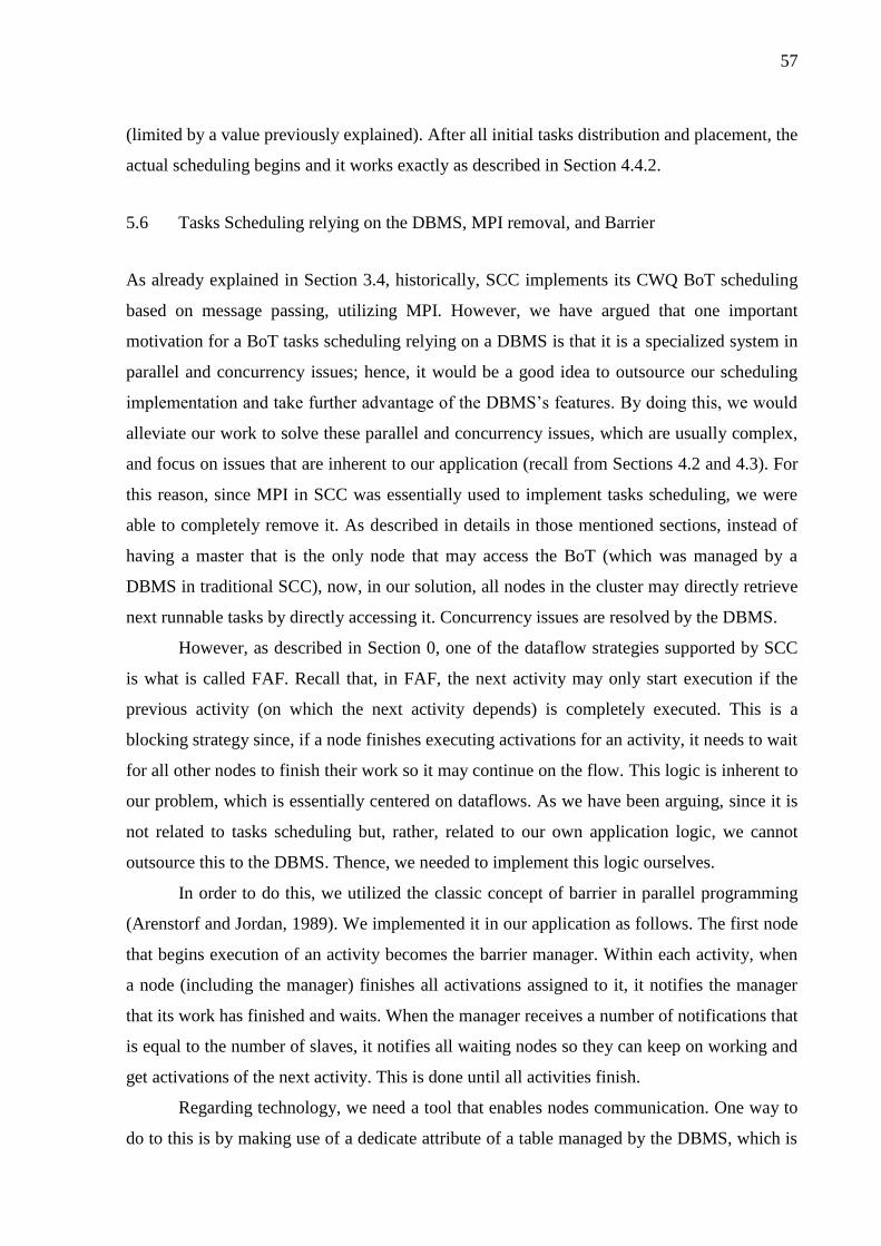
57
(limited by a value previously explained). After all initial tasks distribution and placement, the
actual scheduling begins and it works exactly as described in Section 4.4.2.
Tasks Scheduling relying on the DBMS, MPI removal, and Barrier 5.6
As already explained in Section 3.4, historically, SCC implements its CWQ BoT scheduling
based on message passing, utilizing MPI. However, we have argued that one important
motivation for a BoT tasks scheduling relying on a DBMS is that it is a specialized system in
parallel and concurrency issues; hence, it would be a good idea to outsource our scheduling
implementation and take further advantage of the DBMS’s features. By doing this, we would
alleviate our work to solve these parallel and concurrency issues, which are usually complex,
and focus on issues that are inherent to our application (recall from Sections 4.2 and 4.3). For
this reason, since MPI in SCC was essentially used to implement tasks scheduling, we were
able to completely remove it. As described in details in those mentioned sections, instead of
having a master that is the only node that may access the BoT (which was managed by a
DBMS in traditional SCC), now, in our solution, all nodes in the cluster may directly retrieve
next runnable tasks by directly accessing it. Concurrency issues are resolved by the DBMS.
However, as described in Section 0, one of the dataflow strategies supported by SCC
is what is called FAF. Recall that, in FAF, the next activity may only start execution if the
previous activity (on which the next activity depends) is completely executed. This is a
blocking strategy since, if a node finishes executing activations for an activity, it needs to wait
for all other nodes to finish their work so it may continue on the flow. This logic is inherent to
our problem, which is essentially centered on dataflows. As we have been arguing, since it is
not related to tasks scheduling but, rather, related to our own application logic, we cannot
outsource this to the DBMS. Thence, we needed to implement this logic ourselves.
In order to do this, we utilized the classic concept of barrier in parallel programming
(Arenstorf and Jordan, 1989). We implemented it in our application as follows. The first node
that begins execution of an activity becomes the barrier manager. Within each activity, when
a node (including the manager) finishes all activations assigned to it, it notifies the manager
that its work has finished and waits. When the manager receives a number of notifications that
is equal to the number of slaves, it notifies all waiting nodes so they can keep on working and
get activations of the next activity. This is done until all activities finish.
Regarding technology, we need a tool that enables nodes communication. One way to
do to this is by making use of a dedicate attribute of a table managed by the DBMS, which is

58
used as common mean of communication among all nodes. Since it would be only small
notification messages, queries would not be complex and the amount of data transmitted
would be small. However, nodes would only know that they were notified if they kept
querying the database looking for a data change. For example, a false value would mean that
there is still some node working, so all nodes should wait, and when this value is set to true,
all nodes may continue. Nodes would only acknowledge this value change if they keep
continuously querying the database, which could cause network congestion and downgrade
performance.
Alternatively, a message passing library could be used, like MPI. Nevertheless, MPI is
a robust library and is common in scenarios of data transmission of complex data types and
various data sizes. In our problem, as we argued, we only need to pass notification messages,
which are simple and small. In addition, since SCC is written in Java and uses MPJ18
(known
as MPI for Java), its MPI implementation is more limited and does not support fault tolerance
if a slave node fails, limiting future work for this. Because we were able to completely
remove MPI to implement our tasks scheduling relying on the DDBMS, it is not necessary to
use it just for notification message passing. For this reason, we decided to implement the
barrier as described before using native Java Remote Method Invocation (RMI)19
together
with Java native synchronization directives (wait and notify 20 ) in our current
implementation. Java RMI is known for being simple and easy to use and lightweight, which
fits our barrier needs.
Fault tolerance and load balance 5.7
By using an architecture inspired in WQRM (Section 4.1) and using a DDBMS that allows
replication of the BoT, we increase the availability of the system. If a machine that hosts a
replica of the BoT fails, the entire system does not fail and execution does not stop because
we make of use of the replication feature. We highlight that this failure recovery mechanism
is outsourced and implemented by the DDBMS – which is acknowledged for being efficient
in handling failures (Özsu and Valduriez, 2011) –, and not by our parallel application, which
simplifies our solution.
In addition to the distributed database availability, we also mention fault tolerance for
nodes that do not compose the distributed database in our theoretical architectures (Chapter 4).
18
http://mpj-express.org/
19 http://docs.oracle.com/javase/7/docs/technotes/guides/rmi/
20 http://docs.oracle.com/javase/8/docs/api/java/lang/Object.html#notify()

59
Regarding fault tolerance of the supervisor node, we added a secondary supervisor node to
remove a single point of failure. Regarding fault tolerance of the slave nodes, we explained
that it may be achieved by implementing strategies such as proposed by Anglano et al. (2006).
However, we did not further explain in details how these strategies would apply hence we did
not implement in our current solution. Nevertheless, this is being currently tacked and a more
formal description to incorporate fault tolerance on slaves and on supervisors will be provided
in future work. Furthermore, we described that it is possible to enhance load balance by
verifying whether or not work stealing is advantageous. However, we did not implement it in
our current solution and this is also being provided for future work.

60
6 EXPERIMENTAL EVALUATION
In this chapter, we present the experimental evaluation of our implementation of Architecture
II as described in Section 4.5 and in Chapter 5, where we introduced SciCumulus/C² on a
Distributed Database System (d-SCC).
Regarding hardware, we ran several simulations using Grid500021
, which is composed
of many different clusters distributed in regions in France. In Grid5000, for each region, all
clusters share a file system. The hardware specification of each cluster we used is described in
Table 7. Regarding software, we implemented our solution using MySQL Cluster version
7.4.6. Specifically, we used a compressed TAR file with binaries for generic Linux 64-bit
distribution. We ran most experiments three times and used the average value to present the
results.
Cluster /
Region Processors #Nodes
22
#Cores
per node
Total
cores
Memory
per node Network Storage
Parapide
/ Rennes
Intel Xeon X5570
2.93GHz/6MB 21 8 168 24 GB InfiniBand
SATA II 7200
RPM (RAID-1
and RAID-5)
Graphene / Nancy
Intel Xeon X3440
2.53 GHz 138 4 552 16 GB InfiniBand SATA AHCI
Stremi / Reims
AMD Opteron
6164 HE
1.7 GHz/12MB
42 24 1008 48 GB Gigabit
Ethernet
SATA AHCI &
RAID-5
Table 7 – Hardware specification of clusters in Grid5000
The remainder of this chapter is organized as follows. In Section 6.1, we describe the
workflows we experimented. In Section 6.2, we evaluate architecture variations in order to
analyze the impact of the many different possibilities to configure our architecture. In Section
6.3, we analyze speedup, scalability, and efficiency for different workflow complexities. In
Section 6.4, we show that d-SCC works for a workflow that contains all existing SciWfA
operators (Section 3.1) and we also show the efficiency on running a real bioinformatics
workflow. Finally, we compare d-SCC with the most recent version of SCC in Section 6.5.
Workflows case studies 6.1
We utilized different workflows to evaluate d-SCC; both synthetic and real workflows were
experimented. More specifically, we used the Scientific Workflow Benchmark (SWB)
21
www.grid5000.fr 22
The number of available nodes in these clusters may vary mainly depending on hardware health. Our
experiments were conducted in May 2015 and those are the available nodes we could use in that time.

61
(Chirigati et al., 2012), a synthetic deep water oil exploration workflow (adapted from
(Ogasawara et al., 2011), and SciPhy, a real bioinformatics workflow (Ocaña et al., 2011).
Most of our tests were run using SWB. In SWB, we can generate synthetic data-
centric workflows with a specified number of activities; specify how each activity consumes
and generates data; and control the manipulated data. For example, it is possible to specify a
2-activities Map-Reduce workflow: the first activity consumes and produces one tuple at each
invocation (i.e., it has a Map behavior) and the second activity, dependent on the first activity,
consumes many tuples and produces one at each invocation (i.e., it has a Reduce behavior).
Moreover, we can determine the problem size (i.e., the number of tuples that will be
consumed) as well as the complexity of each computation (i.e., the average elapsed time for
each task).
In this work, we generated two SWB workflows and we are going to call them 1-map
(a simple workflow with one Map activity only) and 3-map (three Map activities, with data
dependency in between). Figure 14 Figure 1shows an activity diagram for each of them. For
each experiment, we varied both problem size and complexity. Since we only utilized SWB
Map activities and each input tuple corresponds to a task that needs to be scheduled and
outputs another tuple, we use the term “number of tasks” instead of “number of tuples” when
we refer to the problem size of either 1-map or 3-map workflows, for readability of this text.
Figure 14 – 1-map and 3-map SWB workflows experimented
In addition to the SWB, we experimented a more complex workflow in order to
investigate whether or not our solution works for all current SciWfA operators (Section 3.1).
The workflow experimented is a synthetic adaptation of a deep water oil exploration
workflow specified by Ogasawara et al. (2011) and is illustrated in the activity diagram in
Figure 15.
In this workflow, some data files are processed and it has 7 activities, including two
that may run in parallel. It is inspired in SWB in the sense that we can control both the
problem size and complexity of tasks.

62
Figure 15 – Deep water oil exploration synthetic workflow (adapted from Ogasawara et al., 2011)
Finally, the last workflow we experimented is SciPhy, a bioinformatics workflow for
phylogenetic analysis of drug targets in protozoan genomes (Ocaña et al., 2011). It also has
many big files manipulated and is illustrated in the activity diagram in Figure 16.
Architecture variations 6.2
Our current implementation of d-SCC is composed of four different roles: dn, dbs ndb_mgmd,
and SCN, as we explained in details in Section 5.3. Moreover, we have argued in Section 5.4.1
that configuring which role each machine will play may directly impact performance. For this
reason, in this section, we want to vary the architecture configuration, measure performance
impact for each configuration, and try to find the most suitable configuration for a given
problem.

63
Figure 16 – SciPhy workflow (extracted from Ocaña et al., 2011).
Experiment 1. In our first experiment, we want to investigate whether or not we
should run, for example, dn nodes or SCN nodes dedicatedly; or if running them altogether on
the same machine has a significant impact. For this, we used the 1-map workflow setting the
problem size to 10 k tasks and average cost to 1 millisecond for tasks. This means that tasks
are extremely light and no much computation is needed for each of them. By doing this, we
stress the database, since there are many very frequent accesses to it, including reads (get next
ready task) and writes (update a completed task status). We only used one node of each role,
i.e., we used at most 4 machines at the same time. We ran on Parapide cluster, which has 8
cores per machine. However, since we wanted to analyze the behavior when all roles were
concurrently running on a same machine, we set the maximum number of threads used both
by SCN and by dne data node) to 4. We ran five variations of the architecture, as described in
Table 8 and the results are shown in Figure 17.

64
Description
Number of
used
machines
I Each machine dedicatedly runs only one process, for each d-SCC role. 4
II SCN runs dedicatedly on a machine; DN also runs dedicatedly on another
machine; and dbs and ndb_mgmd run together on a third machine. 3
III SCN and DN processes run concurrently on a same machine; and dbs and
ndb_mgmd run on another machine. 2
IV SCN dedicatedly on one machine; and all other database nodes (dn, dbs, and
ndb_mgmd) run together on another machine. 2
V All four roles run together, concurrently, on a single machine. 1 Table 8 – Description of each run of Experiment 1.
Figure 17 – Results of Experiment 1. Varying architecture: shared or dedicated nodes?
From the results, we can see that the variation V showed the best execution time, even
though the difference is small. This means that despite having more concurrency in V than in
any other variation, the concurrency overhead is lower than the communication overhead. A
good conclusion from this result is that the variation with the best execution time required the
least number of resources (i.e., only one machine); as a consequence, it points out that we will
be able to use more machines to host SCN processes without significantly impacting
performance, which is the ideal for us. Another important conclusion is related to the idea of
data locality. We could expect that having SCN and dn together on a same machine would
improve performance since less communication would be required to access the database.
However, the result from variation III contradicts this expectation. Comparing variation III, in
which SCN and dn are located on the same machine, with variations II and IV, in which SCN
and dn are in different machines, we see that III has the worst execution time. However,
comparing III with V, in which SCN and DN are also in the same machine, we see that V has a
better performance, suggesting that the communication cost between SCN and dbs also adds a
444 442 518
422 415
0100200300400500600
I.
All dedicated
II.
SCN & DN
dedicated;
dbs & ndb_mgmd
shared
III.
SCN & DN shared;
dbs & ndb_mgmd
dedicated
IV.
SCN dedicated;
dn, dbs, ndb_mgmd
shared
V.
All shared
Execution Time (s)

65
non-negligible overhead. Thence, we may conclude that keeping all roles together has the best
performance especially due to the lowest communication overhead, even though it has the
greatest concurrency overhead. Nevertheless, we need to emphasize that while the machines
have 8 cores, we only used at most 4 cores and forced both SCN and dn to instantiate at most
four threads each process, meaning that concurrency overhead is reduced in all these results
and we are not using all possible cores for SCN. For this reason, we still need more
experiments to have better conclusions.
Experiment 2. This experiment aims to analyze the behavior of our solution in a more
concurrent scenario. To do this, we ran the same workflow with the same configuration as in
Experiment 1 and we used the variation V of our architecture, that is, only one Parapide (8
cores) machine with all roles sharing this same machine. However, instead of using only four
threads at most, we ran two more variations: one with 2 threads (both for the SCN and for the
dn) and another one with eight threads. We reused the result obtained in variation V in Figure
17 for four threads. Ideally, when we double the number of threads, the execution time should
be divided by two. The results are shown in Figure 18, in which the blue line represents d-
SCC’s execution time and the red line represents the ideal execution time. The green bars
represent how far from the ideal d-SCC achieved, in seconds.
Figure 18 – Results of Experiment 2: increasing concurrency
If d-SCC had taken 736 seconds with two threads, the ideal would be if it took 368
seconds (736 * 0.50) with four threads. However, it took 415 seconds (736 * 0.5633), which
represents 47 seconds (or 11.2%) of difference from the ideal execution time. With eight
threads, the ideal time would be 184 seconds (368 * 0.5), but it took 234 seconds (415 *
0.5643), which represents 50 seconds (or 11.4%) from the ideal time. This difference from
47 50
050
100150200250300350400450500550600650700750800
2 threads 4 threads 8 threads
Tim
e (
s)
Difference from ideal d-SCC Ideal

66
ideal is caused due to parallel management overheads. From these results, we mainly want to
show that the overhead caused by concurrency remains close to constant comparing running
on four threads with running on eight threads. This means that difference between the
overheads with four threads and with eight threads is so small (0.2%) that it can be neglected.
In other words, we conclude that we can set the maximum number of threads to be used both
by the SCN and by the dn to be equal to the number of cores in the machine. By doing this, the
efficiency should not be significantly impacted, at least for one single machine. Although it
cannot be generalized for a greater number of machines, this result is meaningful because we
are first mainly interested in finding a good configuration for our architecture rather than
running massive experiments to measure speedup and scalability in larger clusters. Moreover,
we are going to present a similar experiment running on a 960 cores cluster to measure
speedup in next section.
Experiment 3. In this third experiment, we want to analyze the impact of having more
database nodes (dn, dbs, and ndb_mgmd) on the system. For this, we ran our tests on Parapide
cluster, with 21 nodes and 8 cores each (168 cores total). Each of the 21 nodes hosts a SCN
process and the database processes are shared. For example, if we configure 2 dn, 2 dbs, and
2 mgm_ndbd (this is the default configuration recommended to remove single points of failure),
3 machines would run 1 dn, 1 dbs, 1 mgm_ndbd, and 1 SCN concurrently each; the other 18
machines would only run SCN processes, dedicatedly (recall from Section 5.4.1). Regarding
the workflow, we used the 1-map workflow, around 20K tasks with 16 s average task cost.
To present the results, we used the real speedup (Speedup) metric, as defined in Section 2.8.
To calculate the time to execute the workflow with the best (theoretical) sequential program
using one processor, we multiplied the approximate number of tasks by the average task cost.
The workflow execution takes approximately 3.8 days. We also calculated the difference that
each variation has from the best result. The results are shown in Figure 19.

67
Figure 19 – Results of Experiment 3. Varying architecture: changing the number of database nodes.
From the results, comparing the variation I with V, VI, and VII, we can see that
varying either the number of mgm_ndbd or the number of dbs nodes, no much impact is
caused on the system’s performance. Thus, at least for an experiment with similar
characteristics to this Experiment 3, changing the number of mgm_ndbd or dbs has no impact
on performance. Since it has no impact on performance, this result enforces the idea that we
should use at least two nodes for each of these roles so improve availability and remove single
points of failure.
Nevertheless, comparing I with II, II, and IV, we can verify that the number of dn
interferes on the system’s performance. These results lead us to believe that increasing the
number of dn decreases performance. However, we note that the difference on performance
between variations I, II, III is at most 2.1%, which may be considered small; even the
difference in relation to variation IV, which is about 5%, is not very critical. Anyhow, since
we were not expecting the performance to decrease when data nodes were added, we further
investigate the impact of the number of data nodes on a larger cluster.
Experiment 4. In this experiment, we want to evaluate the impact on varying the
number of data nodes (dn) using a larger configuration. For this, we used 138 machines in
Graphene cluster, each with 4 cores, summing 552 cores. We ran the 1-map workflow with
around 20K tasks with 1 s tasks cost average. We note that the tasks cost in this experiment is
considerably lighter than in Experiment 3. By doing this, we want to stress the DDBMS with
many frequent short queries, with both read and write behavior. Similarly to Experiment 3,
0.10%
2.10%
4.10%
6.10%
8.10%
10.10%
12.10%
14.10%
16.10%
18.10%
120
125
130
135
140
145
150
155
160
165
I.1mgm1dbs1dn
II.1ndb_mgmd
1dbs2dn
III.1ndb_mgmd
1dbs3dn
IV.1ndb_mgmd
1dbs4dn
V.1ndb_mgmd
2dbs1dn
VI.1ndb_mgmd
3dbs1dn
VII.2ndb_mgmd
1dbs1dn
Speedup Difference (%)

68
we also used the real speedup metric and the best (theoretical) sequential program using one
processor would take about 6 hours to run. The results are shown in Figure 20. The blue line
represents the speedup varying the number of data nodes when 2 dbs, 2 mgm_ndbd, and 132
SCN were used in a shared way (similarly to Experiment 3); the red square shows the speedup
when 2 dn, 2 mgm_ndbd, 132 SCN, and 8 dbs nodes were used in a shared way; and the
difference between each variation and the best result for this experiment is represented in gray
bars.
Figure 20 – Results of Experiment 4. Varying architecture: increasing number of data nodes.
Conversely, the results of Experiment 4 show that there is not a clear pattern in
relation to adding data nodes as Experiment 3 suggested. Using two data nodes instead of
one resulted in a worse performance, but the difference between these two variations is close
to 2%, similarly to Experiment 3. However, using 4 data nodes had a better performance than
using two and, more surprisingly, using eight data nodes resulted in the best performance.
Using 16 data nodes downgraded performance, but the speedup was not very different than
when using 1 or 4 data nodes. From these results, we can conclude that when there are
multiple short queries (both read and write), using multiple data nodes may alleviate
congestion at the DDBMS, leading to better performance than using a low number of data
nodes, especially in a large cluster with many machines (e.g., 130 machines). We also
highlight that the difference of the performance impact comparing these variations is not very
high: about 5% at most. In addition to analyzing the number of data nodes, we also ran a
single variation on the number of dbs nodes, although it is not presented in Figure 20. We
evaluated the utilization of 8 dbs instead of 2. We could see that using 8 dbs instead of 2 led
to a better performance, even though the difference is small (about 1% in relation to using 2
0.00%
1.00%
2.00%
3.00%
4.00%
5.00%
6.00%76
77
78
79
80
81
82
83
84
1 2 4 8 16
Number of dn
Difference (%) Speedup 2 dbs

69
dbs). This happened most likely because congestion is alleviated when using more ports to
which the 132 SCNs connect.
Experiment 5. In this last experiment for our architecture variation, we want to
analyze differences in relation to the DDBMS configuration. In MySQL Cluster, it is possible
to configure the amount of memory will be used to store data. Moreover, another important
discussion is related to the fact that we can run MySQL Cluster completely in-memory (recall
from the discussion in Section 5.2). Because of these differences, we want to investigate how
d-SCC behaves when the DDBMS configuration varies.
We ran two tests, each to analyze different features of the DDBMS. In the first test (I),
we analyzed data memory capacities using the 1-map workflow with approximately 10 k
tasks, 1 millisecond average task cost, 3 SCN, 1 dn, 1 dbs, 1 mgm_ndbd, and each of them
running dedicatedly (total of 6 machines) on Parapide cluster. In the second test (II), we
compared the performance when running in diskless (in-memory) mode with running using
on-disk checkpoints. We ran the 1-map workflow with approximately 50 k tasks, 2 s average
task cost, 21 SCN, 1 dn, 1 dbs, 1 mgm_ndbd, in a shared way, on Parapide cluster. We highlight
that this was the first time that this amount of tasks was successfully executed in any version
of SCC so far. The results are shown in Figure 21.
I. Varying data memory II. In-memory vs. on-disk
Figure 21 – Results of Experiment 5: varying configuration of the DDBMS.
From the results of Figure 21(I), we can see that varying the data memory capacity has
no significant impact on performance. The results of Figure 21 (II) show that even though
running in diskless mode has 10 s of advantage comparing with on-disk checkpoints mode,
the difference is not critical (1.5%). On-disk checkpoints mode has the advantage of
520524528532536540544548552556560564568
550M 950M 1950M
Data memory
Execution time (s)
0.00%0.50%1.00%1.50%2.00%2.50%3.00%3.50%4.00%4.50%5.00%5.50%6.00%6.50%
700705710715720725730735740745750755760
Diskless On-disk
Execution time (s) Difference (%)

70
persistence, meaning that if a catastrophic disaster happens or if the energy of the entire
cluster fails, the data will remain as long the disk is not damaged. Diskless mode is indeed
faster and we usually save a backup of the database when the workflow execution finishes for
a posteriori data analyses, but if all data nodes fail (i.e., a catastrophic disaster), there will be
data loss even if the disk remains intact.
Therefore, from the five experiments we conducted for the architecture variations, we
can summarize the following conclusions. Using the all-shared mode has shown to deliver the
best performance for the experiments conducted (Experiment 1); setting the maximum
number of threads as equal to the number of cores in the machine delivers a good
performance in a small cluster and more experiments are needed in a larger cluster
(Experiment 2); the number of dbs and ndb_mgmd has no significant impact on performance,
hence we should use at least two of each to improve availability and remove single points of
failure (Experiment 3); many data nodes may either downgrade or improve performance,
depending on the number of SCN and problem complexity (tasks cost) – however, the
difference between a lower number and a greater number of dn is not very high, hence it is
advantageous to use at least two data nodes to remove single points of failure (Experiment 4);
and data memory variation has no big impact and diskless mode has a slightly better
performance than on-disk checkpoints mode (Experiment 5). For these reasons, all of our
next experiments, unless we specifically state differently, were ran using all-shared mode,
number of threads equals to number of cores, at least two database nodes (i.e., 2 dn, 2 dbs,
and 2 ndb_mgmd), and diskless mode.
Scalability, speedup, and efficiency 6.3
In this section, we use known performance metrics to evaluate our system. First, we
evaluate scalability; then, the speedup varying the number of SCN, including different threads
per node; and, finally, we measure the efficiency of d-SCC for different problem complexities.
Experiment 6. In this experiment, we measure scalability using 1-map, 32 s tasks
cost average, on Stremi cluster (24 cores per node). We varied from 5 nodes (120 cores) – 2,5
k tasks to 40 nodes (960 cores) – 20 k tasks. The results are shown in Figures Figure 22 and
Figure 23.

71
Figure 22 – Results of Experiment 6: scalability analyzing execution time.
Figure 23 – Results of Experiment 6: scalability analyzing efficiency.
The ideal is calculated using the concepts about scalability introduced in Section 2.8.
From the figures, we can observe a close-to-constant execution time when we double both
number of nodes and the problem size. Even though the results were farther from the ideal for
960 cores, the efficiency of the system remained over 80% in all executions. Since the number
of cores is relatively large, we consider this a good result.
Experiment 7. To evaluate efficiency when varying complexity (i.e., tasks cost), we
used 3-maps workflow for the first time, with 10 k tasks per map (i.e., 30 k tasks in total). By
doing this, we can also investigate a different known inherent overhead of SCC: caused by the
FAF dataflow execution strategy (recall from Section 0). Regarding hardware, we used all
0
3
6
9
12
15
18
21
24
120 cores2,5 k tasks
240 cores5 k tasks
440 cores10 k tasks
960 cores20 k tasks
Exe
cuti
on
Tim
e (
min
)
Scalability (execution time)
Time (min) Ideal
97% 91%
81%
0%
20%
40%
60%
80%
100%
120 cores2,5 k tasks
240 cores5 k tasks
440 cores10 k tasks
960 cores20 k tasks
Scalability (efficiency)
Efficiency Ideal

72
available machines in Stremi cluster, summing 1,008 cores. We also highlight that this was
the first time that this amount of cores was successfully used to run any version of SCC so far.
The results are shown in Figure 24, where the blue line represents our actual execution
including a contention overhead, which we will explain next; and the red line represents the
efficiency if we removed such overhead.
To measure efficiency, we used the efficiency metric, which is based on the real
speedup metric, as we defined in Section 2.8. To calculate the time to run the workflow
running the best (theoretical) sequential program using one processor, we multiplied the
approximate number of tasks by the tasks cost average, resulting in approximately 9 hours, 35
hours, 69 hours, 138 hours, and 551 hours for tasks cost average 1 s, 8 s, 16 s, and 65 s,
respectively. We highlight that this theoretical sequential time is even farther from reality than
in the previous experiments we ran, because it does not include any overhead, which is
unrealistic in most large parallel systems, and we have a specific significant overhead are we
are going to discuss.
Figure 24 – Results of Experiment 7: varying complexity (tasks cost).
The first conclusion we can get from the results analyzing any of the two lines is that
the greater the complexity of the problem, the better efficiency d-SCC achieves. This is an
expected result and is common in most parallel systems. Indeed, the calculus of efficiency is
directly proportional to the sequential execution time, which is directly proportional to the
tasks cost average; thus, it is expected to achieve such conclusion. Moreover, Raicu et al.
mention that tasks in MTC are short, but in the order of seconds or minutes to run (2008).
Even though our solution suffers due to overheads when computing many very light tasks,
9%
44%
61%
86%
18%
68%
81%
94%
0.00%7.00%
14.00%21.00%28.00%35.00%42.00%49.00%56.00%63.00%70.00%77.00%84.00%91.00%98.00%
1 s 8 s 16 s 65 s
Effi
cie
ncy
Tasks Cost Average
Efficiency with contention overhead
Efficiency without contention overhead

73
such as less than 8 seconds in average, in tasks weighting in the order of minutes, we attain
excellent efficiencies (frequently over 80% in a 1,000 cores cluster).
In addition, comparing the red line with the blue line in Figure 24, we can see that our
system suffers considerably due to the contention overhead caused by the FAF strategy.
Specifically, when all nodes finish their tasks for an activity, all nodes remain blocked until
the supervisor generates new tasks for the next runnable activity and schedules to all SCN,
which will only start their execution when all tasks are generated and scheduled. Thence,
generating tasks per activity causes a contention in current implementation of our solution,
which is more critical for a great number of tasks per activity. This is an inherent overhead in
all implementations of SCC for the FAF strategy.
We can measure this overhead because when all nodes finish their tasks for a certain
activity, the supervisor marks this activity as “finished” and registers in the provenance
database how long this activity took to execute. The SCNs will only start executing tasks for
the next runnable activity when all tasks for this new runnable activity are generated and
scheduled. Thus, the overhead mainly caused by generating and scheduling tasks is given by
the difference between the total workflow execution time and the summation of the execution
time of all activities, as registered in the provenance database.
The red line in Figure 24 shows the efficiency if this overhead did not exist. This
overhead is directly related to the number of tasks rather than the problem complexity; hence,
it remains constant even if the problem complexity varies. For greater complexities, the
execution time is much greater than the overhead, reducing its impact. For this reason, the
difference between the red and blue lines tends to decrease when the complexity increases,
meaning that for computationally complex problems, this overhead may be neglected.
Anyhow, this conclusion is important because it indicates directions for future improvements
in our system. Finally, this overhead may be reduced if tasks were generated in parallel, while
other tasks are still running.
Experiment 8. In the last experiment of this section, we measure speedup when the
number of cores varies. We used the 1-map workflow with 30 k tasks and 32 s tasks cost
average running on Stremi machines (each machine has 24 cores), varying from 120 cores to
960 cores. In addition, we also want to investigate the impact caused by increasing the
concurrency in a larger cluster (recall from the discussion introduced by the results of
Experiment 2). The metric we used was the RelativeSpeedup*, i.e., the Equation (3)
presented in Section 2.8, where = 120 cores. The results are presented in Figure 25.

74
Figure 25 – Results of Experiment 8: speedup varying number of cores.
From the results, we can see that speedup attains almost linear until 240 cores. For 480
cores, the speedup was almost linear for 12 and 24 threads and not far from linear for 48
threads. For 960 cores, the speedup attained close to linear using 12 threads per node and 20%
away from linear using 24 threads per node. We note that setting the maximum number of
threads to be equal to the number of cores gave us a satisfying result (80% of efficiency) in
960 cores.
We can also see that for 48 threads per node, the speedup attained 2.6 points away
from the linear speedup, which represents 34% away from the ideal. However, even though
with 48 threads per node (i.e., 1920 threads in 960 cores) attained the worst speedup, the
execution time is still lower than with 24 threads per node. In fact, the system with 1920
threads ran 1.62 times faster than with 960 threads – the ideal would be 2 times faster.
Analyzing the graph, we can also expect that even with a number of cores greater than
960, the execution time still tends to decrease even with the number of threads twice the
number of cores in the cluster. In these experiments, we did not find a limit for which there
are no more gains if we add more cores or threads to the system. In other words, apparently,
even though the speedup tends to decrease, we will still have gains if we add more cores and
0
1
2
3
4
5
6
7
8
9
5 nodes(120 cores)
10 nodes(240 cores)
20 nodes(480 cores)
40 nodes(960 cores)
Spe
ed
up
12 threads/node 24 threads/node
48 threads/node Linear

75
increase the concurrency in each machine by increasing the number of threads. Thus, if we
want to find this limit, larger experiments in larger clusters are still needed.
Oil & Gas and Bioinformatics workflow 6.4
So far, we have only experimented SWB workflows, which are mainly used to analyze
performance. However, we also need to investigate how d-SCC behaves in more complex
dataflows with added semantics in more relevant domains. For this reason, we use two
workflows. The first is related to oil and gas domain. The main purpose of running this first
workflow is to validate our solution for all current SciWfA operators (Section 3.1). The
second workflow is a real bioinformatics workflow and the main purpose of running it is to
validate our solution in a real scientific scenario.
Experiment 9. We ran a synthetic workflow from oil and gas domain, inspired in deep
water oil exploration scientific applications. Since it is a synthetic workflow, we can predefine
the problem complexity by setting tasks cost weight, which is similar to what we can do in
relation to setting the average tasks cost in SWB workflows. We ran it on 21 Parapide
machines (168 cores in total). Since our main purpose was only to validate d-SCC in a more
complex dataflow containing all SciWfA operators, activities that may run in parallel, and file
manipulations, we did not evaluate performance of the execution. The execution times for
weights 2, 8, and 16 (which just represents complexity; the greater, the more complex) are
shown in Figure 26.
Figure 26 – Execution of Experiment 9: Deep water oil exploration synthetic workflow results
13
41
82
0
15
30
45
60
75
90
2 8 16
Tim
e (
min
)
Weight
Deep Water Oil Exploration Synthetic Workflow Results
Execution Time (min)
76
Experiment 10. For this experiment, we ran a real bioinformatics workflow, known as
SciPhy (recall from Section 6.1). This workflow has 8 activities and some of them are
computationally very complex. We ran on 552 cores Graphene cluster. Through queries to the
database, we were able to find that tasks of the Model Generator activity take more than 30
minutes average each to run. We also found that tasks are considerably balanced. This
scenario is suitable for our solution that works better for complex tasks and also for a more
balanced workload. Moreover, there are many big files manipulated. The workflow
successfully executed in 128 minutes. Through queries to the database, we can estimate a
tasks cost average per activity and come up with an estimate sequential time by multiplying
the tasks cost average by the total number of tasks. The result is 43.6 days and then, given all
this information, we can estimate the real efficiency (efficiency as defined in Section 2.8)
of d-SCC for running SciPhy on 552 cores: 89%.
Finally, we noted a peculiar occurrence when running SciPhy that did not happen
when running any of our previous workflows. When we tried to run using 2 data nodes, as we
have been doing in all experiments in sections Section 6.3 and in the previous experiment of
this current section (Experiment 9), we got an error caused by memory leak. We repeated the
same experiment, with same number of cores, and same dataset, but with 4 data nodes instead,
and it worked successfully. This most likely has happened because d-SCC stores domain data
and SciPhy has data fields with data of significant size. More specifically, phylogenetic trees
are stored in the database and they are big. This result motivates us to look for solutions that
would recognize that a specific big datum is being stored and an extra data node may be
required. Since DDBMSs may implement elastic solutions, such as auto-sharding, which is
the case of MySQL Cluster (Oracle, 2015b), we could add or remove data nodes at runtime
according to the problem needs. This obviously would impact performance, but the workflow
execution would not be interrupted, as happened in our experiment. This, we believe this
could be investigated for future work.
Comparing d-SCC with SCC 6.5
In our last experiments, we are going to compare our implementation of d-SCC with
the most recent version of SCC so far, which uses an architecture with a centralization point at
the master node, as presented in 3 For this, we ran 2 experiments. We ran the exact same
experiment – i.e., same workflow with same input data on same hardware – using both
solutions (d-SCC and SCC) to compare the results.

77
Experiment 11. This is a 1-map workflow on 168 Parapide cores. The results are
shown in Figure 27.
Figure 27 – Results of Experiment 11: comparing d-SCC with SCC on 168 cores.
From the results, we can see that, like d-SCC, SCC also has a better efficiency
(efficiency as defined in Section 2.8) for more complex tasks than for short tasks. Moreover,
analyzing the 2 s results (very frequent short queries), we can see that the centralized
architecture suffers considerably more than our distributed architecture that relies on a
DDBMS. d-SCC showed a gain of 71% over SCC. However, for more complex tasks (16 s
average), the SCNs spend more time with local processing and congestion at centralized points
(e.g., master node and database) is alleviated. In this second scenario, d-SCC almost achieved
a perfect efficiency – we highlight that we used the theoretical real efficiency rather than the
relative efficiency, which would give us an even greater result. The gain over SCC was 15%,
which is considerably lower than those 71% for short tasks. This means that at least for 168
cores and for more complex problems, SCC is still a good solution.
Experiment 12. This is our last experiment. We ran the 3-map workflow, 10 k tasks
per map, on 1008 Stremi cores. By using the 3-map workflow, we can see performance loss
caused by the contention due to the need of waiting for the tasks to be generated and
scheduled.
Efficiency is calculated using the efficiency metric, which is based on a sequential
theoretical time, as defined in Section 2.8. As we discussed in Experiment 7, this efficiency
tends to be farther from reality because it does not include any overhead, which is unrealistic
84%
98%
13%
83%
0%5%
10%15%20%25%30%35%40%45%50%55%60%65%70%75%80%85%90%95%
100%
20 k tasks2 s average task cost
10 k tasks16 s average task cost
Effi
cie
ncy
d-SCC SCC

78
in large parallel systems, and it tends to be unfair due to inherent overheads caused by
contentions due to FAF usage. We could not use the RelativeEfficiency* in this experiment
because running on a smaller number of cores was taking too long and, more importantly, our
main purpose in this experiment was just to see how different the performance between SCC
and d-SCC is. The results are shown in Figure 28.
Figure 28 – Results of Experiment 12: comparing d-SCC with SCC on 1008 cores.
For 1,008 cores, for only 1 s tasks cost average, we can see that both solutions do not
show a good performance. The tasks are so short that generating and scheduling 10 k tasks for
each activity, for all cores, take longer than actually running them. We note that SCC
performs very poorly, considerably worse than d-SCC. For the 16 s experiment, d-SCC
achieves a better performance (more than 51% of gains over SCC), whereas SCC attains at
most 10% of efficiency. Therefore, in all experiments we ran comparing d-SCC with the most
recent version of SCC, we could see significant gains.
12%
1%
10%
0%
10%
20%
30%
40%
50%
60%
1 s 16 s
Effi
cie
ncy
Average Task Cost
Efficiency Comparison
d-SCC SCC

79
7 CONCLUSIONS
This work is inserted in the context of systems that support large-scale computer-based
scientific simulations. Such simulations may be modeled as data-centric scientific workflows,
require HPC, and manipulate a lot of data that need to be carefully managed. We argued that
the control of this data management should not be centralized so performance can be
improved and the HPC environment can be utilized more efficiently. This is an open problem
because current solutions either use a centralized DBMS or use a distributed data control
based on files. The limitations of file-based solutions are mainly due to lack of provenance
storing at runtime, restrictions in analyzing the control information distributed in flat files and
also limitations on provenance generation in the end of execution. To show our points, we
developed a system that not only manages a large volume of data using a distributed database
system, but also relies on such database system to take advantage of its distributed
concurrency control and fault tolerance mechanisms to aid parallel execution of scientific
workflows and remove single points of failure and contention.
Our main contribution is the development of SciCumulus on a Distributed Database
System (d-SCC) built upon Architecture II. Architecture II is a high level architecture in the
sense that it is technology independent – as long as there is a reliable distributed database
system and a parallel workflow management system. It also considers many important aspects
of a large-scale parallel execution of workflows, such as dynamic load balancing and fault
tolerance, taking advantage of a distributed database system.
We concluded that most of the effort spent on developing the tasks scheduling based
on a master-slave architecture was relieved due to using the DDBMS; thence, we could
remove message passing communications that were only being used for tasks’ scheduling and
this facilitated removing a centralized scheduler master. However, we note that a supervisor
node is still necessary for special responsibilities, such as initial tasks distribution, load
balancing, and fault tolerance. Since communication between nodes is needed for this, we still
need to investigate whether it is advantageous not to use other communication strategy rather
than relying on the DDBMS, as we found that using Java RMI would be faster than using the
DDBMS to implement FAF (i.e., a blocking or non-pipeline, recall from Section 0) strategy.
We conducted several experiments to evaluate our implementation of d-SCC. First, we
tried different variations of our architecture to choose the best one to use in most of our latter
experiments. Then, we analyzed scalability and we found that the execution time remains
close to constant when we double the number of cores and the problem size, even running on

80
over 960 cores. We measured speedup and found that by using the number of threads equal to
half of the number of cores, we obtained a speedup very close to linear. Using the number of
threads equal to double of the number of cores, we found that the execution time still tends to
decrease when we increase number of cores, even though speedup was farther from linear.
We did not find a limit for which the execution time stops decreasing when we increase the
number of cores, at least until 960 cores. We also found that the efficiency of our system is
high especially when the problem is complex (i.e., average task cost is high), by frequently
obtaining efficiencies over 80% even on a 1 k cores cluster. We highlight that this was the
first time a system based on SCC ran on such scale of cores and for such problem size (over
50 k tasks). Before that, the centralized solution presented severe limitations to go beyond 500
cores. Moreover, we also experimented our solution in more complex workflows and in a real
bioinformatics workflow. In the end, our last experiments compared d-SCC with SCC and we
found that our solution significantly outperforms the most recent version of SCC, especially
in a 1,000 cores cluster.
This work introduces a first prototype of a distributed architecture to control the
parallel execution of data-centric workflows relying on a DDBMS. We implemented it using
open software (MySQL Cluster), yet scaling up to a considerably large number of cores.
Based on the many good results obtained, we see a lot of opportunities for potential
improvements, in addition to some services that are not currently fully operational. In the
following paragraphs, we point out directions on how our system may be improved and
extended.
We have been claiming that although the underlying d-SCC’s architecture (i.e.,
Architecture II) was theoretically proposed considering many relevant aspects of parallel
execution of large-scale workflows, we did not implement a few parts of this architecture. The
specific parts we proposed and we did not implement are related to dynamic load balancing
through task stealing or any other more sophisticated strategy and failure recovery
mechanisms when either a slave node or the supervisor node faces a hardware failure.
Therefore, this should be implemented in future work. Moreover, the impact on performance
of the solutions for both problems needs to be analyzed.
Furthermore, we argued that the database recovery in case of failure of a database
node is responsibility of the DDBMS. Although we tested our executions forcing a data node
to fail and we found that the execution is indeed not interrupted, this failure recovery
mechanism has impacted the performance of the workflow execution. Thus, we verified that
the single point of failure introduced by a centralized DBMS is removed when a DDBMS is

81
used, but we did not evaluate the impact on performance when a database node fails. This is
an ongoing work jointly with an undergrad student.
In addition to database node failure recovery, one other important aspect to consider is
real time adaptive sharding. This means that when the system acknowledges that too much
data is being stored, an extra data node could be automatically added to the DDBMS so the
execution would not stop. We perceived this necessity when we ran SciPhy, which requires a
lot of domain data to be stored in the database, and the execution of d-SCC was interrupted by
an error and we had to add extra node nodes so it could work (Section 6.4). Thus,
implementing automatic adaptive sharding on d-SCC and analyzing its impact on
performance would be appreciated.
Moreover, we found that the way FAF (Section 3.2) is currently implemented
introduces a significant overhead, especially when dealing with a large MTC problem. The
fact that all processing nodes remain blocked until the supervisor generates tasks and
schedules them so the execution can continue to the next activity (when there is more than
one activity) downgraded performance severely, mainly when the problem’s complexity is
small. Also, FTF (i.e., pipelining) needs to be implemented in d-SCC, which would not
introduce such blocking barrier overhead. The implementation of FTF and improvements on
FAF need to be tackled in future work and this is essential if we want to be able to handle
even larger problems (e.g., millions of tasks), which is currently not viable due to very long
waiting time. Additionally, in Section 2.4.1, we mentioned that determining a good number
value of the chunk size in a BoT may be complex, but may lead to performance improvements
and we could take advantages of the provenance database since we store a lot of relevant
execution data in it. This could be analyzed more deeply in future work. Furthermore,
workflows executed in d-SCC commonly manipulate many big files and we still need
significant improvements on dealing with large domain data files in order to enhance
performance. This is actually being tackled in current work and, for future work, these
efficient domain data management techniques need to be merged into d-SCC.
Finally, d-SCC mainly uses its database with OLTP usage characteristics. Currently,
the DDBMS we chose to implement our architecture is an in-memory database, which
delivered good advantages related to performance. We also showed that using it completely
in-memory, with no checkpoints to the disk, performs considerably well. However, its storage
is limited to the memory of the nodes that compose the DDBMS, which is not a problem
when executing and analyzing one workflow run. Since we want to enable joint rich analyses
of historical big data combining with data of many workflows or workflow executions, we

82
need to load the data from the in-memory database into an on-disk data warehouse. This
should also be tackled in future work.

83
REFERENCES
Altintas, I., Barney, O., Jaeger-Frank, E., (2006), "Provenance Collection Support in the Kepler
Scientific Workflow System", Provenance and Annotation of Data, , chapter 4145, Springer
Berlin, p. 118–132.
Anglano, C., Brevik, J., Canonico, M., Nurmi, D., Wolski, R., (2006), "Fault-aware scheduling for
Bag-of-Tasks applications on Desktop Grids". In: 7th IEEE/ACM International Conference on
Grid Computing, p. 56–63
Arenstorf, N. S., Jordan, H. F., (1989), "Comparing barrier algorithms", Parallel Computing, v. 12, n.
2 (Nov.), p. 157–170.
Benoit, A., Marchal, L., Pineau, J.-F., Robert, Y., Vivien, F., (2010), "Scheduling Concurrent Bag-of-
Tasks Applications on Heterogeneous Platforms", IEEE Transactions on Computers, v. 59, n.
2 (Feb.), p. 202–217.
Bowers, S., McPhillips, T. M., Ludescher, B., (2008), "Provenance in collection-oriented scientific
workflows", Concurrency and Computation: Practice and Experience, v. 20, n. 5, p. 519–529.
Cariño, R. L., Banicescu, I., (2007), "Dynamic load balancing with adaptive factoring methods in
scientific applications", The Journal of Supercomputing, v. 44, n. 1 (Oct.), p. 41–63.
Cario, R. L., Banicescu, I., (2003), "A load balancing tool for distributed parallel loops". In:
Proceedings of the International Workshop on Challenges of Large Applications in
Distributed Environments, 2003Proceedings of the International Workshop on Challenges of
Large Applications in Distributed Environments, 2003, p. 39–46
Carriero, N., Gelernter, D., (1990), How to Write Parallel Programs: A First Course. 1st edition ed.
Cambridge, Mass, The MIT Press.
Chirigati, F., Silva, V., Ogasawara, E., Oliveira, D., Dias, J., Porto, F., Valduriez, P., Mattoso, M.,
(2012), "Evaluating Parameter Sweep Workflows in High Performance Computing". In: 1st
International Workshop on Scalable Workflow Enactment Engines and Technologies
(SWEET’12)SIGMOD/PODS 2012, p. 10, Scottsdale, AZ, EUA.
Cormen, T. H., Leiserson, C. E., Rivest, R. L., Stein, C., (2009), Introduction to Algorithms. Third
Edition ed. The MIT Press.
Costa, F., Oliveira, D. de, Ocaña, K., Ogasawara, E., Dias, J., Mattoso, M., (2012), "Handling Failures
in Parallel Scientific Workflows Using Clouds". In: High Performance Computing,
Networking Storage and Analysis, SC Companion, p. 129–139, Los Alamitos, CA, USA.
Costa, F., Silva, V., de Oliveira, D., Ocaña, K., Ogasawara, E., Dias, J., Mattoso, M., (2013),
"Capturing and Querying Workflow Runtime Provenance with PROV: A Practical Approach".
In: Proceedings of the Joint EDBT/ICDT 2013 Workshops, p. 282–289, New York, NY, USA.
Davidson, S. B., Freire, J., (2008), "Provenance and Scientific Workflows: Challenges and
Opportunities". In: ACM SIGMOD International Conference on Management of Data, p.
1345–1350, New York, NY, USA.
Deelman, E., Gannon, D., Shields, M., Taylor, I., (2009), "Workflows and e-Science: An overview of
workflow system features and capabilities", Future Generation Computer Systems, v. 25, n. 5,
p. 528–540.
Dias, J., (2013), Execução Interativa de Experimentos Científicos Computacionais em Larga Escala,
Universidade Federal do Rio de Janeiro, Tese de Doutorado, PESC/COPPE.
Gadelha, L. M. R., Wilde, M., Mattoso, M., Foster, I., (2012), "MTCProv: a practical provenance
query framework for many-task scientific computing", Distributed and Parallel Databases, v.
30, n. 5-6, p. 351–370.

84
Goble, C., Wroe, C., Stevens, R., (2003), "The myGrid project: services, architecture and
demonstrator". In: Proc. of the UK e-Science All Hands Meeting, p. 595–602, Nottingham,
UK.
Guerra, G. M., Rochinha, F. A., (2009), "Uncertainty quantification in fluid-structure interaction via
sparse grid stochastic collocation method". In: 30th Iberian-Latin-American Congress on
Computational Methods in Engineering, 2009, Buzios
IBM100 - Blue Gene. Disponível em: http://www-
03.ibm.com/ibm/history/ibm100/us/en/icons/bluegene/. Acesso em: 3 Jul 2015.
Lee, K., Paton, N. W., Sakellariou, R., Deelman, E., Fernandes, A. A. A., Mehta, G., (2008),
"Adaptive Workflow Processing and Execution in Pegasus". In: Proceedings of the 3rd
International Conference on Grid and Pervasive Computing, p. 99–106, Kunming, China.
Lima, A. de A. B., (2004), Paralelismo Intra-consulta em Clusters de Bancos de Dados. Tese,
Universidade Federal do Rio de Janeiro, COPPE, Programa de Pós-graduação de Engenharia
de Sistemas e Computação
Mattoso, M., Dias, J., Ocaña, K. A. C. S., Ogasawara, E., Costa, F., Horta, F., Silva, V., de Oliveira,
D., (2015), "Dynamic steering of HPC scientific workflows: A survey", Future Generation
Computer Systems, v. 46 (May.), p. 100–113.
Mattoso, M., Ocaña, K., Horta, F., Dias, J., Ogasawara, E., Silva, V., de Oliveira, D., Costa, F.,
Araújo, I., (2013), "User-steering of HPC workflows: state-of-the-art and future directions".
In: Proceedings of the 2nd ACM SIGMOD Workshop on Scalable Workflow Execution
Engines and Technologies (SWEET), p. 1–6, New York, NY, USA.
Mattoso, M., Werner, C., Travassos, G. H., Braganholo, V., Murta, L., Ogasawara, E., Oliveira, D.,
Cruz, S. M. S. da, Martinho, W., (2010), "Towards Supporting the Life Cycle of Large-scale
Scientific Experiments", International Journal of Business Process Integration and
Management, v. 5, n. 1, p. 79–92.
Mendes, R., Whately, L., de Castro, M. C., Bentes, C., Amorim, C. L., (2006), "Runtime System
Support for Running Applications with Dynamic and Asynchronous Task Parallelism in
Software DSM Systems". In: 18TH International Symposium on Computer Architecture and
High Performance Computing, 2006. SBAC-PAD ’0618TH International Symposium on
Computer Architecture and High Performance Computing, 2006. SBAC-PAD ’06, p. 159–166
Moreau, L., Missier, P., (2013). PROV-DM: The PROV Data Model. Disponível em:
http://www.w3.org/TR/2013/REC-prov-dm-20130430/. Acesso em: 17 Feb 2014.
Ocaña, K. A. C. S., Oliveira, D. de, Ogasawara, E., Dávila, A. M. R., Lima, A. A. B., Mattoso, M.,
(2011), "SciPhy: A Cloud-Based Workflow for Phylogenetic Analysis of Drug Targets in
Protozoan Genomes", In: Souza, O. N. de, Telles, G. P., Palakal, M. [eds.] (eds), Advances in
Bioinformatics and Computational Biology, Springer Berlin Heidelberg, p. 66–70.
Ogasawara, E., Dias, J., Oliveira, D., Porto, F., Valduriez, P., Mattoso, M., (2011), "An Algebraic
Approach for Data-Centric Scientific Workflows", Proceedings of the 37th International
Conference on Very Large Data Bases (PVLDB), v. 4, n. 12, p. 1328–1339.
Ogasawara, E., Dias, J., Silva, V., Chirigati, F., Oliveira, D., Porto, F., Valduriez, P., Mattoso, M.,
(2013), "Chiron: A Parallel Engine for Algebraic Scientific Workflows", Concurrency and
Computation, v. 25, n. 16, p. 2327–2341.
Oliveira, D., (2012), Uma Abordagem de Apoio à Execução Paralela de Workflows Científicos em
Nuvens de Computadores. Tese (doutorado) – UFRJ/ COPPE/ Programa de Engenharia de
Sistemas e Computação, 2012., UFRJ/COPPE
Oliveira, D., Costa, F., Silva, V., Ocaña, K., Mattoso, M., (2014), "Debugging Scientific Workflows
with Provenance: Achievements and Lessons Learned". In: Proceedings of the XXIX Brazilian
Symposium on Databases, Curitiba, Paraná.

85
Oliveira, D., Ogasawara, E., Baião, F., Mattoso, M., (2010), "SciCumulus: A Lightweight Cloud
Middleware to Explore Many Task Computing Paradigm in Scientific Workflows". In:
Proceedings of the 3rd International Conference on Cloud Computing, p. 378–385,
Washington, DC, USA.
Oprescu, A., Kielmann, T., (2010), "Bag-of-Tasks Scheduling under Budget Constraints". In: 2010
IEEE Second International Conference on Cloud Computing Technology and Science
(CloudCom)2010 IEEE Second International Conference on Cloud Computing Technology
and Science (CloudCom), p. 351–359
Oracle, (2015a), MySQL Cluster Evaluation Guide, White Paper, Oracle.
Oracle, (2015b), Guide to Scaling Web Databases with MySQL Cluster, White Paper, Oracle.
Özsu, M. T., Valduriez, P., (2011), Principles of Distributed Database Systems. 3 ed. New York,
Springer.
Paranhos, D., Cirne, W., Brasileiro, F., (2003), "Trading Information for Cycles: Using Replication to
Schedule Bag of Tasks Applications on Computational Grids". In: Proceedings of the Euro-
Par
Raicu, I., (2009), Many-Task Computing: Bridging the Gap Between High-Throughput Computing
and High-Performance Computing. Ph.D. dissertation, The University of Chicago
Raicu, I., Foster, I. T., Zhao, Y., (2008), "Many-task computing for grids and supercomputers". In:
MTAGS 2008MTAGS 2008, p. 1–11
Sahni, S., Thanvantri, V., (1995), Parallel Computing: Performance Metrics and Models
Senger, H., Silva, F. A. B., Nascimento, W. M., (2006), "Hierarchical scheduling of independent tasks
with shared files". In: Sixth IEEE International Symposium on Cluster Computing and the
Grid, 2006. CCGRID 06Sixth IEEE International Symposium on Cluster Computing and the
Grid, 2006. CCGRID 06, p. 8 pp.–51
Silva, D. P. da, Cirne, W., Brasileiro, F. V., (2003), "Trading Cycles for Information: Using
Replication to Schedule Bag-of-Tasks Applications on Computational Grids", In: Kosch, H.,
Böszörményi, L., Hellwagner, H. [eds.] (eds), Euro-Par 2003 Parallel Processing, Springer
Berlin Heidelberg, p. 169–180.
Da Silva, F. A. B., Senger, H., (2010), "Scalability analysis of embarassingly parallel applications on
large clusters". EEE International Symposium on Parallel & Distributed Processing,
Workshops and Phd Forum (IPDPSW), Atlanta, GA, USA.
Da Silva, F. A. B., Senger, H., (2011), "Scalability Limits of Bag-of-Tasks Applications Running on
Hierarchical Platforms", J. Parallel Distrib. Comput., v. 71, n. 6 (Jun.), p. 788–801.
Silva, V., (2014), Uma Estratégia de Execução Paralela Adaptável de Workflows Científicos. Master
Dissertation, Federal University of Rio de Janeiro
Silva, V., Oliveira, D., Mattoso, M., (2014), "SciCumulus 2.0: Um Sistema de Gerência de Workflows
Científicos para Nuvens Orientado a Fluxo de Dados". In: Sessão de Demos do XXIX
Simpósio Brasileiro de Banco de Dados, Curitiba, Paraná.
Simmhan, Y. L., Plale, B., Gannon, D., (2005), A Survey of Data Provenance Techniques, Technical
report, Computer Science Department, Indiana University.
Souza, R., Silva, V., Neves, L., Oliveira, D., Mattoso, M., (2015), "Monitoramento de Desempenho
usando Dados de Proveniência e de Domínio durante a Execução de Aplicações Científicas".
In: Anais do XIV Workshop em Desempenho de Sistemas Computacionais e de Comunicação
(WPerformance), Recife, PE.
TOP 500, (2010), TOP500 Supercomputing Sites, http://www.top500.org/.

86
Walker, E., Guiang, C., (2007), "Challenges in executing large parameter sweep studies across widely
distributed computing environments". In: Workshop on Challenges of large applications in
distributed environments, p. 11–18, Monterey, California, USA.
Wozniak, J. M., Armstrong, T. G., Wilde, M., Katz, D. S., Lusk, E., Foster, I. T., (2013), "Swift/T:
Large-Scale Application Composition via Distributed-Memory Dataflow Processing". In:
Proceedings of the 13th IEEE/ACM International Symposium on Cluster, Cloud and Grid
Computing (CCGrid), p. 95–102