convection in fluids 9789048124329
DESCRIPTION
TRANSCRIPT

Convection in Fluids

FLUID MECHANICS AND ITS APPLICATIONSVolume 90
Series Editor: R. MOREAUMADYLAMEcole Nationale Supérieure d’Hydraulique de GrenobleBoîte Postale 9538402 Saint Martin d’Hères Cedex, France
Aims and Scope of the Series
The purpose of this series is to focus on subjects in which fluid mechanics plays afundamental role.
As well as the more traditional applications of aeronautics, hydraulics, heat andmass transfer etc., books will be published dealing with topics which are currentlyin a state of rapid development, such as turbulence, suspensions and multiphasefluids, super and hypersonic flows and numerical modeling techniques.
It is a widely held view that it is the interdisciplinary subjects that will receiveintense scientific attention, bringing them to the forefront of technological advance-ment. Fluids have the ability to transport matter and its properties as well as totransmit force, therefore fluid mechanics is a subject that is particularly open tocross fertilization with other sciences and disciplines of engineering. The subject offluid mechanics will be highly relevant in domains such as chemical, metallurgical,biological and ecological engineering. This series is particularly open to such newmultidisciplinary domains.
The median level of presentation is the first year graduate student. Some texts aremonographs defining the current state of a field; others are accessible to final yearundergraduates; but essentially the emphasis is on readability and clarity.
For other titles published in this series, go towww.springer.com/series/5980

R.Kh. Zeytounian
Convection in Fluids
A Rational Analysis and Asymptotic Modelling

R.Kh. ZeytounianUniversité des Science et Technologies de LilleFrance
ISBN 78-90-481-2432-9 e-ISBN 78-90-481-2433-6
Library of Congress Control Number: 2009931692
© 2009 Springer Science+Business Media, B.V.No part of this work may be reproduced, stored in a retrieval system, or transmittedin any form or by any means, electronic, mechanical, photocopying, microfilming, recordingor otherwise, without written permission from the Publisher, with the exceptionof any material supplied specifically for the purpose of being enteredand executed on a computer system, for exclusive use by the purchaser of the work.
Printed on acid-free paper
Springer is part of Springer Science+Business Media (www.springer.com)
Springer Dordrecht Heidelberg London New York 9 9
There is no better wayfor the derivation of significant
model equations than rational analysisand asymptotic modeling

Contents
Preface and Acknowledgments . . . . . . . . . . . . . . . . . . . . . . . . . . . . . . . . . xi
1 Short Preliminary Comments and Summary ofChapters 2 to 10 . . . . . . . . . . . . . . . . . . . . . . . . . . . . . . . . . . . . . . . . . . 11.1 Introduction . . . . . . . . . . . . . . . . . . . . . . . . . . . . . . . . . . . . . . . . . . 11.2 Summary of Chapters 2 to 10 . . . . . . . . . . . . . . . . . . . . . . . . . . . 3References . . . . . . . . . . . . . . . . . . . . . . . . . . . . . . . . . . . . . . . . . . . . . . . 26
2 The Navier–Stokes–Fourier System of Equations andConditions . . . . . . . . . . . . . . . . . . . . . . . . . . . . . . . . . . . . . . . . . . . . . . . 292.1 Introduction . . . . . . . . . . . . . . . . . . . . . . . . . . . . . . . . . . . . . . . . . . 292.2 Thermodynamics . . . . . . . . . . . . . . . . . . . . . . . . . . . . . . . . . . . . . 302.3 NS–F System for a Thermally Perfect Gas . . . . . . . . . . . . . . . . 352.4 NS–F System for an Expansible Liquid . . . . . . . . . . . . . . . . . . . 382.5 Upper Free Surface Conditions . . . . . . . . . . . . . . . . . . . . . . . . . . 402.6 Influence of Initial Conditions and Transient Behavior . . . . . . 492.7 The Hills and Roberts’ (1990) Approach . . . . . . . . . . . . . . . . . . 52References . . . . . . . . . . . . . . . . . . . . . . . . . . . . . . . . . . . . . . . . . . . . . . . 54
3 The Simple Rayleigh (1916) Thermal Convection Problem . . . . 553.1 Introduction . . . . . . . . . . . . . . . . . . . . . . . . . . . . . . . . . . . . . . . . . . 553.2 Formulation of the Starting à la Rayleigh Problem for
Thermal Convection . . . . . . . . . . . . . . . . . . . . . . . . . . . . . . . . . . . 603.3 Dimensionless Dominant Rayleigh Problem and the
Boussinesq Limiting Process . . . . . . . . . . . . . . . . . . . . . . . . . . . . 623.4 The Rayleigh–Bénard Rigid-Rigid Problem as a
Leading-Order Approximate Model . . . . . . . . . . . . . . . . . . . . . . 66
vii

viii Contents
3.5 Second-Order Model Equations Associated with the RBShallow Convection Equations (3.25a–c) . . . . . . . . . . . . . . . . . . 71
3.6 Second-Order Model Equations Following from the Hillsand Roberts Equations (2.70a–c) . . . . . . . . . . . . . . . . . . . . . . . . . 73
3.7 Some Comments . . . . . . . . . . . . . . . . . . . . . . . . . . . . . . . . . . . . . . 76References . . . . . . . . . . . . . . . . . . . . . . . . . . . . . . . . . . . . . . . . . . . . . . . 82
4 The Bénard (1900, 1901) Convection Problem, Heated fromBelow . . . . . . . . . . . . . . . . . . . . . . . . . . . . . . . . . . . . . . . . . . . . . . . . . . . 854.1 Introduction . . . . . . . . . . . . . . . . . . . . . . . . . . . . . . . . . . . . . . . . . . 854.2 Bénard Problem Formulation, Heated from Below . . . . . . . . . . 924.3 Rational Analysis and Asymptotic Modelling . . . . . . . . . . . . . . 1044.4 Some Complements and Concluding Remarks . . . . . . . . . . . . . 110References . . . . . . . . . . . . . . . . . . . . . . . . . . . . . . . . . . . . . . . . . . . . . . . 130
5 The Rayleigh–Bénard Shallow Thermal Convection Problem . . 1335.1 Introduction . . . . . . . . . . . . . . . . . . . . . . . . . . . . . . . . . . . . . . . . . . 1335.2 The Rayleigh–Bénard System of Model Equations . . . . . . . . . . 1385.3 The Second-Order Model Equations, Associated to RB
Equations . . . . . . . . . . . . . . . . . . . . . . . . . . . . . . . . . . . . . . . . . . . . 1435.4 An Amplitude Equation for the RB Free-Free Thermal
Convection Problem . . . . . . . . . . . . . . . . . . . . . . . . . . . . . . . . . . . 1445.5 Instability and Route to Chaos in RB Thermal Convection . . . 1525.6 Some Complements . . . . . . . . . . . . . . . . . . . . . . . . . . . . . . . . . . . 162References . . . . . . . . . . . . . . . . . . . . . . . . . . . . . . . . . . . . . . . . . . . . . . . 169
6 The Deep Thermal Convection Problem . . . . . . . . . . . . . . . . . . . . . 1736.1 Introduction . . . . . . . . . . . . . . . . . . . . . . . . . . . . . . . . . . . . . . . . . . 1736.2 The Deep Bénard Thermal Convection Problem . . . . . . . . . . . . 1746.3 Linear – Deep – Thermal Convection Theory . . . . . . . . . . . . . . 1766.4 Routes to Chaos . . . . . . . . . . . . . . . . . . . . . . . . . . . . . . . . . . . . . . 1826.5 Rigorous Mathematical Results . . . . . . . . . . . . . . . . . . . . . . . . . . 189References . . . . . . . . . . . . . . . . . . . . . . . . . . . . . . . . . . . . . . . . . . . . . . . 193
7 The Thermocapillary, Marangoni, Convection Problem . . . . . . . 1957.1 Introduction . . . . . . . . . . . . . . . . . . . . . . . . . . . . . . . . . . . . . . . . . . 1957.2 The Formulation of the Full Bénard–Marangoni
Thermocapillary Problem . . . . . . . . . . . . . . . . . . . . . . . . . . . . . . 2007.3 Some ‘BM Long-Wave’ Reduced Convection Model Problems 205
Convection in Fluids ix
7.4 Lubrication Evolution Equations for the DimensionlessThickness of the Film . . . . . . . . . . . . . . . . . . . . . . . . . . . . . . . . . . 214
7.5 Benney, KS, KS–KdV, IBL Model Equations Revisited . . . . . . 2187.6 Linear and Weakly Nonlinear Stability Analysis . . . . . . . . . . . . 2407.7 Some Complementary Remarks . . . . . . . . . . . . . . . . . . . . . . . . . 252References . . . . . . . . . . . . . . . . . . . . . . . . . . . . . . . . . . . . . . . . . . . . . . . 260
8 Summing Up the Three Significant Models Related with theBénard Convection Problem . . . . . . . . . . . . . . . . . . . . . . . . . . . . . . . 2638.1 Introduction . . . . . . . . . . . . . . . . . . . . . . . . . . . . . . . . . . . . . . . . . . 2638.2 A Rational Approach to the Rayleigh–Bénard Thermal
Shallow Convection Problem. . . . . . . . . . . . . . . . . . . . . . . . . . . . 2658.3 The Deep Thermal Convection with Viscous Dissipation . . . . 2708.4 The Thermocapillary Convection with Temperature-
Dependent Surface Tension . . . . . . . . . . . . . . . . . . . . . . . . . . . . . 272References . . . . . . . . . . . . . . . . . . . . . . . . . . . . . . . . . . . . . . . . . . . . . . . 275
9 Some Atmospheric Thermal Convection Problems . . . . . . . . . . . 2779.1 Introduction . . . . . . . . . . . . . . . . . . . . . . . . . . . . . . . . . . . . . . . . . . 2779.2 The Formulation of the Breeze Problem via the Boussinesq
Hydrostatic Approximation . . . . . . . . . . . . . . . . . . . . . . . . . . . . . 2799.3 Model Problem for the Local Thermal Prediction – A Triple
Deck Viewpoint . . . . . . . . . . . . . . . . . . . . . . . . . . . . . . . . . . . . . . . 2929.4 Free Convection over a Curved Surface – A Singular Problem 2989.5 Complements and Remarks . . . . . . . . . . . . . . . . . . . . . . . . . . . . . 304References . . . . . . . . . . . . . . . . . . . . . . . . . . . . . . . . . . . . . . . . . . . . . . . 322
10 Miscellaneous: Various Convection Model Problems . . . . . . . . . . 32510.1 Introduction . . . . . . . . . . . . . . . . . . . . . . . . . . . . . . . . . . . . . . . . . . 32510.2 Convection Problem in the Earth’s Outer Core . . . . . . . . . . . . . 32710.3 Magneto-Hydrodynamic, Electro, Ferro, Chemical, Solar,
Oceanic, Rotating, Penetrative Convections . . . . . . . . . . . . . . . 33110.4 Averaged Integral Boundary Layer Approach: Non-
Isothermal Case . . . . . . . . . . . . . . . . . . . . . . . . . . . . . . . . . . . . . . . 34510.5 Interaction between Short-Scale Marangoni Convection and
Long-Scale Deformational Instability . . . . . . . . . . . . . . . . . . . . . 34910.6 Some Aspects of Thermosolutal Convection . . . . . . . . . . . . . . . 35410.7 Anelastic (Deep) Non-Adiabatic and Viscous Equations for
the Atmospheric Thermal Convection (à la Zeytounian) . . . . . 35910.8 Flow of a Thin Liquid Film over a Rotating Disk . . . . . . . . . . . 363

x Contents
10.9 Solitary Waves Phenomena in Bénard–MarangoniConvection . . . . . . . . . . . . . . . . . . . . . . . . . . . . . . . . . . . . . . . . . 369
10.10 Some Comments and Complementary References . . . . . . . . . 377References . . . . . . . . . . . . . . . . . . . . . . . . . . . . . . . . . . . . . . . . . . . . . . . 384
Subject Index . . . . . . . . . . . . . . . . . . . . . . . . . . . . . . . . . . . . . . . . . . . . . . . . 391

Preface and Acknowledgments
The purpose of this monograph is to present a unified (analytical) approachto the study of various convective phenomena in fluids. Such fluids aremainly considered to be thermally perfect gases or expansible liquids. Asa consequence, the main driving force/mechanism is the buoyancy force(Archimedean thrust) or temperature-dependent surface tension inhomo-geneities (Marangoni effect). But we take into account, also, in the generalmathematical formulation – for instance, in the Bénard problem for a liquidlayer heated from below – the effect of an upper deformed free surface, abovethe liquid layer. In addition, in the case of atmospheric thermal convection,the Coriolis force and stratification effects are also taken into account.
My main motivation in writing this book is to give a rational, analytical,analysis of the main physical effects in each case, on the basis of the fullunsteady Navier–Stokes and Fourier (NS–F) equations – for a Newtoniancompressible/dilatable, viscous and heat-conductor fluid, coupled with theassociated initial and boundary (lower) and free surface (upper) conditions.
This, obviously, is a difficult but necessary task, if we wish to construct arational modelling process, keeping in mind a coherent numerical simulationon a high speed computer.
It is true that the ‘physical approach’ can produce valuable qualitativeanalyses and results for various significant and practical convection phenom-ena. Unfortunately, an ad hoc physical approach would not be able to pointthe way for a consistent derivation of approximate (leading order) modelproblems which could be used for a quantitative numerical calculation; thisis true especially because such an approach would be unable to provide a ra-tional, logical method for the derivation of an associated second-order modelproblem with various complementary (e.g., to a usual Boussinesq approxi-
xi

xii Preface and Acknowledgments
mation) effects (such as viscous dissipation and free surface deformation) tobuoyancy-driven Rayleigh–Bénard thermal convection.
Concerning this physical approach, which is necessary for full compre-hension of the nature of convection, we refer the reader to Physical Hydro-dynamics, by E. Guyon, J.-P. Hulin, L. Petit and C.D. Mitescu, publishedby Oxford University Press, Oxford, 2001. On the other hand, in the reviewpaper ‘Convective Instability: A Physicist’s Approach’, by Ch. Normand, Y.Pomeau and M.G. Velarde, published in Reviews of Modern Physics, vol. 49,no. 3, pp. 581–624, July 1977, a number of apparently disparate problemsfrom fluid mechanics are thoroughly considered under the unifying headingof natural convection.
Actually, various technologically complex convective flow problems arefrequently resolved via massive numerical computations on the basis of adhoc approximate models. It should not be surprising that such a numericalapproach leads to a simulation which has little practical interest because ofits inconsistency with the experimental results! If one is to use this numericaltechnique, it is necessary – at least from my point of view – that a rationalconsistent approach is adopted to make sure that:
“if, in the fluid dynamics starting equations and boundary/initial condi-tions, a term is neglected, then, it is essential to be convinced that sucha term is really much smaller than the terms retained in the derivedapproximate model’s equations and conditions”.
It should be noted that such a rational consistent approach, with an asymp-totic modelling process, assures the possibility to obtain – via various sim-ilarity rules between small or large non-dimensional parameters governingdifferent physical effects – some criteria for testing the range of validity ofthese derived approximate models.
My profound conviction is that a rational/analytical-asymptotic modellingis a necessary theoretical basis for research into the solution of a difficultnonlinear problem, before a numerical computation. Both the numerics andmodelling are useful and strongly complementary. Our present project is indirect line with our consistent scientific attitude:
Putting a clear emphasis on rigorous – but not strongly formal mathematical– development of consistent approximate model problems for different kindsof convective flows.
However, to acknowledge a certain point of view, I know that some readersdo not care much for this rigor and simply want to know: ‘what are the rel-

Convection in Fluids xiii
evant model equations and boundary conditions for their problems?’ Such areader will find a special chapter, namely Chapter 8, which is a kind of ‘gen-eral advice’ where, for each of the three particular convections we consider –shallow, deep, and Marangoni – I specify the physical conditions, the limita-tions for the main parameters, which govern, respectively: buoyancy, viscousdissipation and free surface/surface tension effects. In addition, the leadingorder model equations and associated boundary conditions for these threecases are specified, and the reader can find our recommendations for takinginto account the corresponding second-order, non-Boussinesq, free surfacedeformation and viscous dissipation effects.
The first, main kind of convective transport (convection) I discuss in thismonograph is called natural or free convection, meaning that the fluid (liquidor atmospheric air) flow is a response to a force acting within the body of thefluid. The force is most often gravity (buoyancy) but there are circumstanceswhere some other agency, such as surface (temperature-dependent) tensionor other forces – for example the Coriolis force – play a significant or even aprimary role.
Convection, as a physical phenomenom, is thoroughly discussed in thesurvey paper by M.G. Velarde and Ch. Normand, ‘Convection’, publishedin Scientific American, vol. 243, no. 1, pp. 92–108, July 1980. In this sur-vey paper, ‘Convection’, the spontaneous upwelling of a heated fluid, canbe understood only by untangling the intricate relations among temperature,viscosity, surface tension and other characteristics of the considered fluidflow problem. Natural (or free) convection is defined in contradistinction toforced convection, where the fluid motion is induced by the effect of a hetero-geneous temperature field or by a relief as in atmospheric, mesoscale motion,for instance, a lee waves regime (adiabatic and non-viscous) downstream ofa mountain!
I have made every effort to present a logical organization of the mater-ial and it should be stressed that there is no physics involved, but rather anextensive use of dimensional analysis, similarity rules, asymptotics of NS–F equations with boundary conditions and calculus. Until this is undertood,though even now it is possible (in part!), it will be difficult to convince adetached and possibly skeptical reader of their value as an aid to understand-ing!
A valuable – again, at least from my point of view – feature of my rational(but not rigorously mathematical) approach is the possibility to derive, con-sistently, not only the leading-order, limiting first-order, approximate modelproblem, but also the associated second-order model which takes into ac-count complementary effects.
xiv Preface and Acknowledgments
This gives, curiously, the possibility in many cases to clarify (as thisis described in Chapter 8) the conditions required for the validity of theusual derived leading-order model problems. For just this purpose, via non-dimensional analysis and the appearance of reduced parameters/numbers, itis necessary to adequately take into account various similarity rules.
This book has been written for final year undergraduates and graduatestudents, postgraduate research workers and also for young researchers influid mechanics, applied mathematics and theoretical/mathematical physics.However, it is my conviction that anyone who is interested in a systematicand logical account of theoretical aspects of convection in fluids, will find inthe present monograph various answers concerning an analytical approachin modelling of the related problems.
The choice of the nine chapters, Chapters 2 to 10, is summarized in Chap-ter 1 and their ordering is, at least from my point of view, quite natural. Thepresentation of the material, the relative weight of various arguments and thegeneral style reflects the tastes of the author and his knowledge and abilitygained over 50 years of research work in fluid mechanics.
In Chapter 1, devoted to a ‘Short Preliminary Comments and Summaryof Chapters 2 to 10’, the reader can find an ‘extended abstract’ of the fullmaterial included in the other nine chapters. All the papers and books citedin Chapters 1 to 10 are listed at the end of these chapters. In many cases thereader can find (in the sections ‘Comments and Complements’ before thereferences in some chapters) various information concerning recent (up to2008) results linked with convection in fluids.
Fluid mechanics has spawned a myriad of theoretical research projectsby numerous fluid dynamicists and applied mathematicians. The richness ofthe area can be seen in the major questions surrounding Rayleigh-Bénardconvection, which itself is an approximate problem resulting from the ap-plication of asymptotic/perturbation techniques to the full NS–F equationsusing Boussinesq approximation for a weakly expansible/dilatable liquid. Inthe relatively recent survey paper by E. Bodenchatz, W. Pesh and G. Ahlers,published in Annual Review of Fluid Mechanics, vol. 32, pp. 709–778, 2000,the reader can find the main results for this RB convection that have beenobtained during the past decade, 1990–2000, or so.
I should like to thank to Dr. Christian Ruyer-Quil (from the University ofParis Sud – Orsay) with who I have had during the last years many discus-sions related to the modelling of thin film problems and also to Dr. B. Scheid(from the Université Libre de Bruxelles, Begium) who gave me the oportu-nity to visit the ‘Microgravity Reseach Center’ of Professor J.C. Legros.

Convection in Fluids xv
My thanks to Professor Manuel G. Velarde, Director of the Unidad deFluidos in ‘Instituto Pluridisciplinar UCM’ de Madrid (Spain), for his hospi-tality in his Unidad de Fluidos and with whom I have had many discussionsand collaborations, relative to Marangoni thermocapillary convection, dur-ing the years 2000–2004. Together we organized a Summer Course held atCISM (Undine, Italy) in July 2000, devoted to ‘Interfacial Phenomena andthe Marangoni Effect’ and edited in collaboration a CISM Courses and Lec-tures (No. 428), published by Springer, Wien/New York in 2002.
Finally, my gratitude to Professor René Moreau, as the Series Editor of‘FMIA’, who has given me various useful criticism and suggestions, andrecommended this book for publication by Springer, Dordrecht.
R.Kh. ZeytounianParis, April 2008

Chapter 1Short Preliminary Comments and Summary ofChapters 2 to 10
1.1 Introduction
During the years 1967–1972 at the ONERA, then 1972–1996 at the Uni-versity of Lille I, and later, following retirement from this University in theyears 1997–2002, at home in Paris-Center, I published more than 20 papersdevoted to convection in fluids. As an Introduction to this book, I wish togive a short discourse on six of these papers that I consider as particularlyvaluable results. The interested reader will find all of these quoted papersand books listed at the end of this chapter.
A first valuable result was obtained in 1974, namely a rigorous justifi-cation, based on an asymptotic approach for low Mach numbers, of the fa-mous Boussinesq approximation and the rational derivation of the associ-ated Boussinesq equations [1]. In chapter 8 of [2], a monograph publishedin 1990 and devoted to the asymptotic modelling of atmospheric flows, thereader can find a careful derivation and analysis of these Boussinesq equa-tions, valid for atmospheric low velocity motions – the so-called small Machnumber/hyposonic case.
A second interesting result was published in 1983 in a short note [3],where it seems that, for the first time, there appeared a rigorous formulationof the Rayleigh–Bénard (RB) thermal convection problem using asymptotictechniques. This result opened the door for a consistent derivation of thesecond-order approximate model equations for Bénard, heated from below,thermal convection (see, for instance, in this book, Sections 3.5 and 3.6,Section 5.3 and 8.1).
In 1989, by means of a careful dimensionless analysis of the exact, full,Bénard problem of thermal instability for a weakly expansible liquid heatedfrom below, as a third new result [4], I show also that:
1

2 Short Preliminary Comments and Summary of Chapters 2 to 10
. . . if you have to take into account, in model approximate equationsfor the Bénard problem, the viscous dissipation term in the tempera-ture equation, then it is necessary to replace the classical shallow con-vection, (RB) equations, by a new set of equations, called the ‘deepconvection’ (DC-Zeytounian) equations.
These deep convection equations contain a new ‘depth parameter’ and arederived and analyzed in this book in Chapter 6.
A fourth result, which appear as a quantitative criterion for the valuationof the importance of buoyancy in the Bénard problem, is the following alter-native [5], obtained in 1997:
Either the buoyancy is taken into account, and in this case the free-surface deformation effect is negligible and we rediscover the classi-cal Rayleigh–Bénard (RB) shallow convection rigid-free approximateproblem or, the free-surface deformation effect is taken into accountand, in such a case at the leading-order approximation for a weaklyexpansible fluid, the buoyancy does not give a significant effect in theBénard–Marangoni (BM) thermocapillary instability problem.
This alternative is related to the value of the reference Froude number
Frd = (ν0/d)/(gd)1/2,
based on the thickness d of the liquid layer, magnitude of the gravity g andconstant kinematic viscosity ν0, and for
RB problem: Frd � 1,
while for the
BM problem: Frd ≈ 1 ⇒ d ≈ (ν20/g)
1/3 ≈ 1 mm.
The small effect of the viscous dissipation, in the RB model problem, givesa complementary criterion for the thickness d (see Chapters 3, 4 and 5).
A fifth result is linked with my written lecture notes [6] for the SummerCourse held at CISM (Udine, Italy, and coordinated by M.G. Velarde andmyself) in July 2000, where I discussed ‘Theoretical aspects of interfacialphenomena and Marangoni effect – Modelling and stability’.
Although significant understanding has been achieved, yet surface-tension-gradient-driven BM convection flows, still deserve further studies;in particular, the case of a single Biot number for a conduction motionless

Convection in Fluids 3
state and also for the convection regime (the Biot number is the dimension-less parameter linked with the heat transfer across an upper, liquid-ambientair, free surface) poses many problems, especially in the case when this sin-gle Biot number is assumed ‘vanishing’ in the convection regime!
Concerning the Boussinesq approximation, we refer here to my re-cent paper [7], ‘Foundations of Boussinesq approximation applicable to at-mospheric motions’, published in 2003 (see Chapter 9 in the present book)as my sixth, and last result, to be mentioned here.
However, on the other hand, in addition to the research mentioned aboveon convection and Boussinesq approximation, during the years 1991–1995I used a rather new approach to obtain various asymptotically significantmodels for ‘nonlinear long surface waves in shallow water’ and ‘solitons’.The results of these ‘investigations’ were written about in two survey papers[8] and [9] in 1994 and 1995 and also in the 1993 monograph [10].
1.2 Summary of Chapters 2 to 10
Chapter 2 is devoted to Navier–Stokes and Fourier (NS-F) systems of equa-tions which are derived from the basic relations for momentum, mass, andenergy balance, according to a continuum regime:
ρdudt
= ρf + ∇ · T, (1.1a)
dρ
dt= −ρ(∇ · u), (1.1b)
ρde
dt= −∇ · q + T · (∇u). (1.1c)
These three equations (1.1a–c) are the classical conservation laws at anypoint of continuity in a fluid domain V , where the velocity vector u, the den-sity ρ and the specific internal energy e have piecewise-continuous boundedderivatives.
In equation (1.1a), f is the body force per unit mass (usually, in convectionproblems, the gravity force) and T is the stress tensor (with the componentsTij ). In equation (1.1c), q is the heat flux vector with components qi .
The time derivative, with respect to material motion, is written as
d
dt:= ∂
∂t+ u · ∇, (1.1d)

4 Short Preliminary Comments and Summary of Chapters 2 to 10
and
∇ = ∂
∂xi, i = 1, 2, 3,
withx1 = x, x2 = y, x3 = z.
To obtain the classical, NS–F, Newtonian, system of equations, from (1.1a–c), for u, ρ, p (mechanical pressure) and T (absolute temperature), it is nec-essary to assume the existence of two equations of state and two constitutiverelations for the stress tensor T and heat flux vector q.
Concerning the equations of state, I consider, mainly, two cases.First, the case of a thermally perfect gas with two equations of state:
e = CvT , (1.2a)
p = RρT , (1.2b)
where Cv is the specific heat at constant volume v (= 1/ρ), and R is theperfect gas constant – the mechanical pressure p being then in a fluid at restand in the framework of the Newtonian-classical fluid mechanics, such that(see also (1.4a)):
Tij = −pδij , (1.2c)
withδij = 1, if i = j and δij = 0 for i �= j, (1.2d)
where δij , is the well-known Kronecker delta tensor.Second, the case of an expansible liquid when
e = E(v, p), (1.3a)
with the following Maxwell relation (see Section 2.1):
Cp − Cv = T
(∂p
∂T
)v
(∂v
∂T
)p
, (1.3b)
where Cp is the specific heat for a constant pressure p.In Section 2.2, we give more detailed information concerning ‘thermody-
namics’ for an expansible liquid.In the framework of Newtonian (classical) fluid mechanics (see, for is-
tance, the very pertinent basic survey paper by Serrin [11]), if we assumethat a thermally perfect gas and an expansible liquid can be modelled asa viscous Newtonian fluid, then we can write for the components Tij , of the

Convection in Fluids 5
stress tensor T, the following (first) constitutive relation (originally obtained,by de Saint-Venant [12]):
Tij = −pδij + 2µ[dij − (1/3)�δij ], (1.4a)
where the dij are the components of the rate of strain tensor D(u), such that
dij = (1/2)
[∂ui
∂xj+ ∂uj
∂xi
], (1.4b)
� ≡ dkk = ∇ · u, (1.4c)
and µ is the shear viscosity and depends on thermodynamic pressure P (dif-ferent, in general, from the mechanical pressure p), and also of the absolutetemperature T .
However, here, because the Stokes relation,
λ ≡ −(2/3)µ, (1.4d)
which gives the second coefficient of viscosity λ, as a function of µ, has beentaken into account in the above constitutive relation (1.4a), we have that
P ≡ p. (1.4e)
Now, if for the heat flux, q, in equation (1.1c), we adopt as (a second)constitutive relation the classical Fourier law:
q = −k∇T , (1.5)
where k is the thermal conductivity coefficient, then with (1.4a) and (1.5),we have the possibility to write the energy balance equation (1.1c), for thespecific internal energy e, in the following form:
ρde
dt= Tij
(∂ui
∂xj
)+ ∂
∂xi
(k∂T
∂xi
), (1.6a)
or
ρde
dt= −p�+ 2µ[dij dij − (1/3)�2] + ∂
∂xi
(k∂T
∂xi
), (1.6b)
where(2µ/ρ)[dij dij − (1/3)�2] ≡ � (1.7)
is the rate of (viscous) dissipation of mechanical energy, per unit mass offluid, due to viscosity.

6 Short Preliminary Comments and Summary of Chapters 2 to 10
With the first of equations of state (1.2a) for a thermally perfect gas, sincewe have e = CvT , it is easy (see Section 2.3) to obtain from (1.6b) anevolution equation for the temperature T , the specific heat, Cv, being usuallyassumed a constant.
However, for an expansible liquid – in the case of a thermal convectionproblem – obtaining such a result is more subtle because the density is thena function of pressure and temperature (see Section 2.4). In Section 2.5 thereader can find the free surface jump conditions associated with the NS–Fsystem of equations for an expansible liquid and, in Sections 2.6 and 2.7,a discussion concerning the initial conditions and a short derivation of theHills and Roberts equations [34] (see also below the summary concerningChapter 6).
In Chapter 3 we revisit the thermal convection problem considered byLord Rayleigh in 1916 [13]. Stimulated by the Bénard [14] experiments LordRayleigh, in his pioneer 1916 paper, first formulated the theory of convectiveinstability of a layer of fluid: an expansible liquid, with as equation of state:
ρ ≡ ρ(T ), (1.8a)
between two horizontal rigid planes, and derive in an ad hoc manner thefamous Rayleigh–Bénard, (RB), instability model problem.
The starting (approximate) equations in the Rayleigh paper are thoseobtained by Boussinesq [15] and are valid when
“the variations of density are taken into account only when they modify theaction of gravity force g (= −gk)”
k is the unit vector for the vertical axis of z.The (weakly) expansible liquid layer, for which the fixed thickness is d,
is assumed to be bounded by two infinite fixed, rigid horizontal planes, atz = 0 and z = d, such that
T = Tw at z = 0 (1.8b)
andT = Td at z = d, (1.8c)
such that�T = Tw − Td > 0. (1.8d)
It is well known that the main parameter that drives the thermal convectionis the Grashof (Gr) number or Rayleigh (Ra) number,

Convection in Fluids 7
Gr = α(Td)�T gd3
ν2d
, (1.9a)
Ra = α(Td)�T gd3
νdκd, (1.9b)
where Ra ≡ PrGr, with as Prandtl number
Pr = νd
κd. (1.9c)
In (1.9a–c), νd and κd are, respectively, the constant (at T = Td )kinematic viscosity νd [= µ(Td)/ρ(Td)] and thermal diffusivity κd =[k(Td)/ρ(Td)Cv(Td)].
The coefficient of thermal expansion [when ρ ≡ ρ(T )] of the liquid isdefined as
α(T ) = −(1/ρ(T ))[
dρ(T )
dT
]. (1.9d)
On the other hand,
ε = α(Td)�T ≈ 5 × 10⁻³, (1.10a)
which is a small parameter (the expansibility number) for many liquids, andis our main small parameter in derivation of an approximate limit for themodel (RB) problem.
In particular, when the square of the Froude number (based on the thick-ness d)
Fr2d ≡ (νd/d)
2
gd, (1.10b)
is small – Fr2d � 1 – we obtain for the thickness of the liquid layer, d, the
following constraint (a lower bound):
d �(ν2d
g
)1/3
≈ 1 mm, (1.11)
The main result (according to Zeytounian [5]) in Chapter 3 is that
the Boussinesq, shallow convection model equations, with the buoy-ancy as main driving (Achimedean) force, are significant, rational-consistent equations in the framework of the classical RB instability,rigid-rigid problem if, and only if, we assume simultaneously the small-ness of both numbers, ε (expansibility) and F2
d (square of the Froudenumber).

8 Short Preliminary Comments and Summary of Chapters 2 to 10
In such a case, the limiting process, à la Boussinesq,
Gr = ε
Fr2d
fixed, when ε ↓ 0 and Fr2d ↓ 0, (1.12)
is the RB limiting process and, as a consequence, for the validity of the RBmodel problem (à la Rayleigh, derived in Chapter 3) it is necessary to con-sider a thicker weakly expansible liquid layer than a very thin film layer ofthe order of the millimetre, as is the case for the Bénard–Marangoni thermo-capillary instability problem (considered in Chapter 7).
An important moment in a consistent derivation of shallow convection,RB equations, is strongly linked with an evaluation of the effect of the vis-cous dissipation, �, in energy balance (see, for instance, (1.6b) with (1.7)).
Namely, this evaluation gives an upper bound for the thickness, d, of theweakly expansible liquid layer. More precisely, on the basis of a dimension-less analysis and the derivation of a ‘dominant’ energy equation for the di-mensionless temperature
θ = (T − Td)
�T, �T = Tw − Td, (1.13)
we obtain that the role of the viscous dissipation is linked with the following‘dissipation number’:
Di∗ = Di
2Gr, (1.14)
which was introduced by Turcotte et al. in 1974 [16], where
Di ≡ εBo. (1.15)
In (1.15), the ratio Bo, of two ‘thicknesses’, d and Cv(Td)�T/g, plays therole of a Boussinesq number:
Bo = gd
Cv(Td)�T. (1.16)
The reader can find a discussion concerning the account of viscous heatingeffects in a paper by Velarde and Perez Cordon [17]. We observe that, in our1989 paper [4], the parameter Di is in fact the product of two parameters:
ε (which is � 1) by Bo (assumed � 1),
and has been denoted by δ (assumed O(1)), which is our ‘depth’ parameter.In Section 3.4, the rigid-rigid, à la Rayleigh, RB problem is derived and in
Sections 3.5 and 3.6, the second-order model equations associated with RB

Convection in Fluids 9
shallow convection equations are obtained in a consistent way. Section 3.7is devoted to some comments. Concerning the derivation and analysis ofthe deep thermal convection equations, which take into account the termproportional to dissipation parameter Di∗, see Chapter 6 in this monograph.
Chapter 4 has a central place in the present monograph, and the readercan find (in Section 4.2) a full mathematical/analytical rational formulationof the Bénard, heated from below, convection problem and its reduction toa system of non-dimensional ‘dominant’ equations and conditions, wherevarious reduced parameters are present. In particular, this non-dimensionaldominant system takes into account:
(i) the temperature-dependent surface tension,(ii) the static basic conduction state,(iii) the deformation of the free surface.(iv) the heat transfer at the free surface via an usual ‘Newton’s cooling law’.
This free surface, simulated by the equation
z = d + ah(t, x, y) ≡ H(t, x, y),
in a Cartesian co-ordinate system (O; x, y, z) in which the gravity vector g =−gk acts in the negative z direction and where a is an amplitude, separatesthe weakly expansible liquid layer from ambient motionless air at constanttemperature TA and constant atmospheric pressure pA, having a negligibleviscosity and density.
We observe that the problem of the upper, free-surface condition for thetemperature (in fact, an open problem) is discussed in various parts of thismonograph. The temperature-dependent surface tension σ (T ) is assumed de-creasing linearly with temperature. Thus:
σ (T ) = σ (Td)− γσ (T − Td), (1.17a)
where
γσ = −(
dσ (T )
dT
)d
(1.17b)
is the constant rate of change of surface tension with temperature, which ispositive for most liquids.
However we observe that several authors instead of (T −Td) use (T −TA),where TA is the constant ambient air temperature above the deformable freesurface of the weakly expansible liquid layer. In such a case, instead of θgiven by (1.13), these authors introduce another dimensionless temperature:

10 Short Preliminary Comments and Summary of Chapters 2 to 10
� = (T − TA)
(Tw − TA). (1.17c)
With (1.17a, b) the surface tension effects are expressed by the following twonon-dimensional parameters:
We = σdd
ρdν2d
, (1.18a)
Ma = γσd�T
ρdν2d
, (1.18b)
which are, respectively, the Weber and Marangoni numbers, which play animportant role in Bénard–Marangoni (BM) thermocapillary instability prob-lems.
We observe again that, in (1.17a, b) Td is the constant temperature on thefree surface, in the purely, static motionless, basic conduction state, which isobviously (no convection) the level z = d when the (conduction) tempera-ture is simply:
Ts(z) = Tw − βsz (1.19a)
with
βs = −dTs(z)
dz> 0. (1.19b)
Obviously, at z = d,Td = Tw − βsd
or
βs = (Tw − Td)
d≡ �T
d, (1.19c)
and the above Marangoni number Ma, according to (1-18b), is expressed viathe above βs ,
Ma = γσd2βs
ρdν2d
. (1.19d)
Concerning Newton’s cooling law of heat transfer, written for the basic,motionless conduction temperature Ts(z), we have
k(Td)dTs(z)
dz+ qs(Td)[Ts(z)− TA] = 0, at z = d; (1.20)
when in a basic, motionless conduction state, the thermal conductivity coef-ficient
k = k(Td) = const.

Convection in Fluids 11
In (1.20), qs(Td) is the unit thermal surface conductance (also a constant).From (1.20) with (1.19a) we obtain:
βs = Bis(Td)
[(Td − TA)
d
], (1.21a)
or
βs =[
Bis(1 + Bis)
] [(Tw − TA)
d
], (1.21b)
where
Bis(Td) = dqs(Td)
k(Td), (1.22)
is the conduction Biot number (at T = Td = const.).The lower heated plate temperature, T = Tw ≡ Ts (z = 0), being a given
data in the classical Bénard, heated from below, convection problem, theadverse conduction temperature gradient βs appears [according to (1.21b)]as a known function of the temperature difference (Tw−TA), where TA < Twis the known constant temperature of the passive (motionless) air far abovethe free surface, when Bis(Td) is assumed known, thanks to (1.21a). But forthis it is necessary that the constant (conduction) heat transfer qs(Td) (theunit thermal surface conductance) was considered as a data! If so,
Ts(z = d) = Td(≡ Tw − βsd)
is the assumed to be determined.One should realize that βs is always different from zero in the framework
of the Bénard convection problem heated from below!
As a consequence, the above, defined by (1-22), constant conduction Biotnumber is also always different from zero: Bis(Td) �= 0; it characterizes the‘Bénard conduction’ effect and makes it possible to determine the purelystatic basic temperature gradient βs .
This seemingly trivial remark is in fact important, because in the mathemat-ical formulation of the full Bénard, heated from below, convection problem,with a deformable free surface, we do not have the possibility to work onlywith a single conduction, Bis(Td) �= 0, Biot number. Namely, necessarily asecond (but certainly variable) convective Biot number,
Biconv = dqconv
k(Td), (1.23a)
12 Short Preliminary Comments and Summary of Chapters 2 to 10
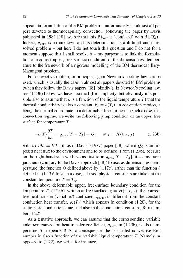
appears in formulation of the BM problem – unfortunately, in almost all pa-pers devoted to thermocapillary convection (following the paper by Davispublished in 1987 [18], we see that this Biconv is ‘confused’ with Bis(Td)).Indeed, qconv is an unknown and its determination is a difficult and unre-solved problem – but here I do not touch this question and I do not for amoment suppose that I shall resolve it – my purpose is to link the formula-tion of a correct upper, free-surface condition for the dimensionless temper-ature to the framework of a rigorous modelling of the BM thermocapillary-Marangoni problem.
For convective motion, in principle, again Newton’s cooling law can beused, which is usually the case in almost all papers devoted to BM problems(when they follow the Davis papers [18] ‘blindly’). In Newton’s cooling law,see (1.23b) below, we have assumed (for simplicity, but obviously it is pos-sible also to assume that k is a function of the liquid temperature T ) that thethermal conductivity is also a constant, kd ≡ k(Td), in convection motion, nbeing the normal coordinate to a deformable free surface. In such a case, in aconvection regime, we write the following jump condition on an upper, freesurface for temperature T :
−k(T )∂T∂n
= qconv[T − TA] +Q0, at z = H(t, x, y), (1.23b)
with ∂T /∂n ≡ ∇T · n, as in Davis’ (1987) paper [18], where Q0 is an im-posed heat flux to the environment and to be defined! From (1.23b), becauseon the right-hand side we have as first term qconv[T − TA], it seems morejudicious (contrary to the Davis approach [18]) to use, as dimensionless tem-perature, the function � defined above by (1.17c), rather than the function θdefined in (1.13)! In such a case, all used physical constants are taken at theconstant temperature T = TA.
In the above deformable upper, free-surface boundary condition for thetemperature T , (1.23b), written at free surface, z = H(t, x, y), the convec-tive heat transfer (variable?) coefficient qconv, is different from the constantconduction heat transfer, qs(Td) which appears in condition (1.20), for thestatic basic conduction state, and also in the conduction, constant, Biot num-ber (1.22).
As a tentative approach, we can assume that the corresponding variableunknown convection heat transfer coefficient, qconv, in (1.23b), is also tem-perature, T , dependent! As a consequence, the associated convective Biotnumber is also a function of the variable liquid temperature T . Namely, asopposed to (1.22), we write, for instance,

Convection in Fluids 13
Biconv(T ) = dqconv(T )
k(Td). (1.23c)
But another approach may be also:
Biconv(H) = dqconv(H)
k(Td), (1.23d)
where H = d + ah(t, x, y) is the full (variable) thickness of the convectiveliquid layer. Indeed, the assumption concerning necessity of the introductionof a variable convective heat transfer coefficient is present in the pioneeringpaper by Pearson (1958) [19], where a small disturbance analysis is carriedout.
If in a conduction (motionless, steady) phase, when the temperature Tdis constant (uniform) along the flat free surface z = d, we have obviously,q = qs(Td) = const.; unfortunately this is no longer true in a thermocapillaryconvective regime, because the dimensionless temperature (θ or �) at theupper, deformable, free surface, z = H(t, x, y), varies from point to point!
In reality, the heat transfer coefficient and Biot number in a convectionregime depend, in general, on the free surface properties of the fluid, the un-known motion of the ambient air near the free surface and also to the spatio-temporal structure of the temperature field – see the discussion in Joseph’s1976 monograph [20, part II], and in Parmentier et al.’s 1996, very pertinentpaper [21], where the problem of two Biot numbers is very well discussed.
As a consequence of the ‘co-existence’ of two Biot numbers, conductionand convection, the formulation of the upper, free-surface boundary condi-tion, derived from the jump condition (1.23b), for θ , is significantly differentthan the Davis condition derived in [18]. With two Biot numbers the cor-rect condition is given by (1.24c), and the Davis condition is given by (1.25)when, as in Davis [18] we confuse Bis(Td) with Biconv! Indeed Davis, in hispaper [18], during the derivation from (1.23b) of a dimensionless conditionat deformable upper, dimensionless free surface [t ′ = t/(d2/νd), x′ = x/d,y′ = y/d],
H ′ = H
d⇒ z′ = 1 + ηh′(t ′, x′, y′), with η = a/d, (1.23e)
for θ , given by (1.13), to bind oneself to use the relation (1.21a) which givesthe possibility to replace the difference of the temperaure (Tw−Td) by (Tw−TA), namely,
dβs = Bis(Td)(Td − TA) ⇒ (Td − TA)
(Tw − Td=
[1
Bis(Td)
]. (1.24a)

14 Short Preliminary Comments and Summary of Chapters 2 to 10
In such a case, Davis rewrites the above jump condition (1.23b) in thefollowing dimensionless form (see Davis [18, p. 407, formula (3.2)]):
∂θ
∂n′ + Biconv
{[(Td − TA)
(Tw − Td)
]+ θ
}+ Q0
kβs= 0 at z′ = 1 + ηh′(t ′, x′, y′).
(1.24b)From (1.24b), with (1.24a), we derive the desired correct condition, if we
do not confuse Biconv (from Newton’s cooling law, (1.23b), for the convec-tion) with Bis(Td), which arises from the relation (1.21a), rewritten above as(1.24a).
Namely we obtain the following correct condition:
∂θ
∂n′ +[
Biconv
Bis(Td)
]{1 + Bis(Td)θ} + Q0
kβs= 0, at z′ = 1 + ηh′(t ′, x′, y′).
(1.24c)But this above correct condition, (1.24c), is unfortunately not the conditionthat Davis derived in [18]! Only after the confusion (by a curious oversight?)of the conduction Biot number, Bis(Td), with the Biot number for the convec-tion Biconv, in (1.24c), and the consideration of a single ‘surface Biot numberB’, did Davis obtain the upper, free-surface condition for the dimensionlesstemperature θ in the dimensionless form:
∂θ
∂n′ + 1 + Bθ = 0, at z′ = 1 + ηh′(t ′, x′, y′), (1.25)
when Q0 = 0 – the precise (conduction or convection) meaning of the B, in(1.25), being unclear!
It should be observed also that the appearance of a single, constant (in fact,only, conduction) Biot number, simultaneously in a conduction motionlessbasic state (which makes it possible to evaluate the corresponding value ofthe purely static basic temperature gradient βs , according to (1.21b)) andin formulation of the thermocapillary convective Marangoni flow problem –via the upper, at z′ = H ′(t ′, x′, y′), condition (1.25) for θ – leads to a veryambiguous situation.
This is a particularly unfortunate case, when this single (in fact conduc-tion) Biot number is taken equal to zero. From this point of view, the resultsof Takashima’s 1981 paper [22], concerning the linear Marangoni convec-tion – in the case of a zero (conduction?) Biot number – must be accuratelyreconsidered (at least in a logical derivation process).
This two Biot problem deserves, obviously, further attention and I hopethat the reader will consider our present discussion as a first step in the ex-planation of this intriguing question.

Convection in Fluids 15
Section 4.3 is devoted to a rational analysis and asymptotic modellingof the above Bénard, heated from below, convection problem, taking intoaccount mainly the results of Section 4.2.
In the last section of Chapter 4 (Section 4.4), we give some complementsand concluding remarks concerning, first, again, the upper, free-surface con-dition for the temperature, then, a second discussion is devoted to long-scaleevolution of thin liquid films (the models based on the long-wave approxima-tion are also considered in Chapter 7), and a third short discussion concernsthe various problems related to liquid films (falling down an inclined or ver-tical plane or inside a vertical circular or else hanging below a solid ceilingand also over a substrate with topography). Finally, we see now that threesignificant convection cases deserve interest, namely:
1. shallow-thermal, when Fr2d � 1,
2. deep-thermal, when Di ≡ εBo ≈ 1,3. Marangoni-thermocapillary, when Fr2
d ≈ 1,
which are considered in Chapters 5, 6 and 7.Indeed, a fourth special case,
4. ultra-thin film, when Fr2d � 1,
deserves also a careful investigation – for instance when in a long-wave ap-proximation: d/λ � 1 ⇒ (d/λ)Fr2
d ⇒ F 2 = λ2dg/νA2 = O(1) – but in the
present book we do not discuss this fourth case. In Chapter 8 the above threecases are also considered.
In Chapter 5, Section 5.2, we first derive the usual shallow RB convectionmodel equations, where the main driving force is buoyancy – this derivationbeing performed via the RB limiting process (1.12) as in Chapter 3. In Sec-tion 5.3, second-order model equations associated to RB equations are de-rived. But, in Chapter 5, unlike Chapter 3, a new (curious) problem emergesbecause of the presence of the term (η/Fr2
d)h′ [where the ratio, η = a/d is
the upper, free-surface amplitude parameter, see (1.23e)], in the dominant(dimensionless) free surface upper boundary condition for (p − pA), rewrit-ten with dimensionless pressure π defined by the relation
π =(
1
Fr2d
){[(p − pA)/gdρd] + z′ − 1}, z′ = z/d. (1.26)
As a consequence:
The free surface upper boundary condition for the dimensionless pressureπ is asymptotically (at the leading order) consistent with the RB limitingprocess (1.12), only for a small free surface amplitude, η � 1, such that:

16 Short Preliminary Comments and Summary of Chapters 2 to 10
η
Fr2d
≡ η∗ ≈ 1, (1.27a)
whenη and Fr2
d both tend to zero. (1.27b)
In this case, for the RB model limit problem, according to (1.12), the upper,free-surface boundary conditions, at the leading order, are written for a non-deformable free surface z′ = 1.
Besides, in the framework of a rational formulation of the RB leading-order model problem, a new amazing result is the derivation – at the leadingorder – from the jump condition for the pressure (see, for instance, the re-lation (2.42a) in Chapter 2) of an equation for the deformation of the freesurface, h′(t ′, x′, y′). Namely, for the unknown h′(t ′, x′, y′) we obtain thepartial differential equations
∂2h′
∂x′2 + ∂2h′
∂y′2 −(η∗
We∗
)h′ = −
(1
We∗
)πsh, at z′ = 1, (1.28a)
whereWe∗ = ηWe ≈ 1, (1.28b)
because usually the Weber number is large, We � 1.In the right-hand side of (1.28a), the term πsh (t ′, x′, y′, z′ = 1), together
with ush and θsh, is known when the solution (subscript ‘sh’) of the RB shal-low convection problem is obtained.
Thus, we verify that, for a rational derivation of the RB, shallow rigid-freethermal convection model problem, it is necessary to assume the existenceof three similarity relations:
ε
Fr2d
= Gr, (1.29a)
andη
Fr2d
≡ η∗, (1.29b)
η
Cr= We∗, (1.29c)
with four simultaneous limiting processes:
ε ↓ 0, Fr2d ↓ 0, η ↓ 0, (1.29d)
and the crispation (or capillary) number

Convection in Fluids 17
Cr ≡ 1
We↓ 0. (1.29e)
Owing only to our rational analysis and asymptotic approach is it possibleto derive on the one hand, equation (1.28a) for deformation of the free sur-face, h′(t ′, x′, y′), and, on the other hand, a second-order consistent modelproblem – associated with the leading-order RB model problem – whichtakes into account the second-order (proportional to Fr2
d � 1) terms (seeSections 3.5 and 3.6, and Section 5.3).
Indeed, in the RB model problem we have the possibility to partially takeinto account the Marangoni and Biot effects on the upper, non-deformable,free surface. Recently (in 1996, see [23]) such a model problem has beenconsidered by Dauby and Lebon, but without any justification or discussion.
Finally, we observe that in the case of the RB shallow convection modelproblem, when the dimensionless parameter Bo, defined by (1.16), is fixedand of the order of unity,
d≈Cv(Td)�T
g, (1.30a)
we can write (or identify) the squared Froude number with a low squared(‘liquid’) Mach number M2
L, via the chain rule:
Fr2d ≈ (νd/d)
2
Cv(Td)�T=
[(νd/d)
(Cv(Td)�T )1/2
]2
≡ M2L. (1.30b)
Therefore, for our weakly expansible liquid, instead of Fr2d , we can use M2
L,which is the ratio of the reference (intrinsic) velocity UL = νd/d to thepseudo-sound speed, CL = [Cv(Td)�T ]1/2, for the liquid. The above ap-proach has been used recently in our 2006 book (see [24, chapter 7, sec-tion 7.2.3]).
In Section 5.4, an amplitude equation à la Newel–Whitehead, is asymp-totically derived and Section 5.5 is devoted to instability and route to chaos(to ‘temporal’ turbulence), in RB thermal shallow convection, via the threemain scenarios (Ruelle–Takens, Feigenbaum and Pomeau–Manneville) inthe framework of a finite-dimensional dynamical system approach. The lastsection of that chapter, Section 5.6, is devoted to some comments.
Chapter 6 is devoted to the so-called ‘deep thermal convection’ problem,first discovered in 1989 [4], and analyzed by Zeytounian, Errafyi, Charki,Franchi and Straughan during the years 1990–1996 (see [25–32]). Indeed,the above discussion concerning the RB problem (in Chapter 5) shows thatthe RB model problem is valid (operative) only in a (Boussinesq) liquid layerof thickness d such that [see (1.11) and (1.30a)]:
18 Short Preliminary Comments and Summary of Chapters 2 to 10
(ν2d
g
)1/3
� d ≈ Cv(Td)�T
g≡ dsh, (1.31a)
because, according to (1.15), only when Bo ≈ 1 do we have a small dissipa-tion number such that
Di ≈ ε, (1.31b)
and the term proportional to εBo (linked with the viscous dissipation ) dis-appears, at the leading order, when we derive RB model equations via theBoussinesq limiting process (1.12).
Therefore, on the contrary, the condition:
Bo � 1, such that Di ≡ εBo fixed, of the order unity, (1.31c)
characterizes the deep convection (DC) problem.Obviously, (1.31c) is a direct consequence of the relation (1.14) for Di∗,
because in limiting process (1.12), the Grashof number, Gr, is fixed and oforder unity.
In such a case, with (1.31c), the dissipation number Di∗ is also of theorder unity and the viscous dissipation term is operative equally with thebuoyancy term in thermal convection equations. As a consequence, in thedeep convection problem we have for the thickness d, of the liquid layer, theestimate
d ≈ Cv(Td)
gα(Td)≡ ddepth, (1.32)
and
Di ≡ gα(Td)d
Cv(Td)(1.33)
is our depth parameter (denoted by δ in our 1989 paper, see [4]).The formulation of a deep convection ( DC) problem is necessary when
the thickness d of the liquid layer satisfies the constraint (1.32), Di, givenby (1.33), being a significant parameter. Finally, the deep convection modelproblem is derived, in a rational way, via the following, DC, limiting process:
Gr = ε
Fr2d
fixed and Di ≡ εBo fixed, (1.34a)
whenε ↓ 0, Fr2
d ↓ 0 and Bo ↑ ∞. (1.34b)
In two papers [25,26], by Errafyi and Zeytounian the reader can find a lin-ear theory for deep convection and various routes to chaos in the frameworkof deep convection unsteady two-dimensional equations.

Convection in Fluids 19
On the other hand, in two papers [27, 28] by Charki and Zeytounian, thereader can find the derivation of a Lorenz deep system of equations and theLandau-Ginzburg amplitude equation for deep convection. Then, in threepapers by Charki [29–31], the reader will find also some rigorous mathemat-ical results – stability, existence and uniqueness of the solution for the initialvalue problem and for the steady-state problem.
The deep convection problem is derived in Section 6.2, and in Section 6.3a linear theory is presented. Section 6.4 is devoted to an investigation of threemain routes to chaos (mentioned above) and in Section 6.5 some commentsare given concerning the rigorous mathematical results of Charki, Richard-son and Franchi and Straughan.
Concerning these deep convection equations, we observe that in the pa-per by Franchi and Straughan [32], a nonlinear energy stability analysisof our 1989 deep convection equations is given. Finally, in the book byStraughan [33], the reader can find a derivation and discussion concerningdeep convection in the framework of the theory of Hills and Roberts [34].Unfortunately the equations derived by these authors in an ad hoc manner(with some ‘compressible’ effects) are not consistent (see also Section 3.6).
Chapter7 is devoted entirely to thermocapillary – Marangoni convection– the so-called Bénard–Marangoni (BM) – thin film problem.
It is now well known (mainly thanks to Pearson [17]) that Bénard convec-tive cells are primarily induced by the temperature-dependent surface tensiongradients resulting from the temperature variations along the free surface (theso-called Marangoni/thermocapillary effect) – in the leading order, both thebuoyancy and viscous dissipation effects are neglected, but free surface de-formations are taken into account, the model equations are those which gov-ern an imcompressible viscous liquid – the temperature field being presentvia the upper, free-surface conditions where appears the Marangoni, Weberand Biot (convective) numbers.
On the other hand, the classical Rayleigh–Bénard (RB) thermal convec-tion problem (considered in Chapter 5) is produced mainly by the buoyancy– the influence of a deformable free surface being neglected at the leadingorder for a weakly expansible liquid in a not very thin layer, according to(1.31a).
Naturally, in the general/full nonlinear (NS–F) convection, heated frombelow Bénard problem for an expansible viscous liquid – considered fromthe start in Chapter 4 – in the derived dimensionless dominant equations andupper, free-surface conditions, both buoyancy and Marangoni, Weber, Bioteffects are operative. But for a weakly expansible liquid, in a thin (of order ofthe millimetre) layer, when Fr2
d ≈ 1, the deformable free surface influence is

20 Short Preliminary Comments and Summary of Chapters 2 to 10
operative and the temperature-dependent surface tension, via the Marangoninumber, has a driving effect. The buoyancy force, however, is negligible atthe leading order.
As a consequence: it is not consistent (from an asymptotic point of view, atleast in the leading-order, limiting, case) to take into account fully the abovethree effects – thermocapillarity, buoyancy and free surface deformation –simultaneously, for a weakly expansible viscous liquid.
The buoyancy is operative only in the RB thermal convection rigid-freeproblem. Conversely, the effects linked with the deformable upper, free sur-face are operative only in the Bénard–Marangoni (BM) thermocapillary thinfilm problem.
The main cause of this curious (leading-order) aspect of the full Bénard,heated from below, problem for a weakly expansible liquid, is the conse-quence of the presence of Fr2
d in the definition (as a denominator) of theGrashof number,
Gr = α(Td)�T
Fr2d
, (1.35a)
where the expansibility number is assumed always to be a small parameter,
ε = α(Td)�T � 1! (1.35b)
The only possibility for a full account of the deformation of the free sur-face, separating the weakly expansible liquid layer from the ambient, pas-sive, motionless air, is directly related to the condition
Fr2d ≈ 1 (1.35c)
or
d ≈(ν2d
g
)1/3
= dBM ≈ 1 mm. (1.35d)
In this case, it is not necessary to assume (in upper, free-surface, dominantconditions derived in Chapter 4) that the free surface amplitude parameter, η,is a small parameter [see (1.27a) and (1.27b)], as is the case for the RB modelproblem. But, with (1.35c), the buoyancy term, proportional to the Grashofnumber, is in fact of the order of the small expansibility parameter, ε, anddoes not appear in the leading-order, limiting case (ε → 0), in equationsgoverning the BM problem.
The BM model problem, derived at the leading order, from the full domi-nant Bénard problem (with upper, free-surface, dominant conditions) is for-mulated in Chapter 4, via the following incompressible limiting process:
Convection in Fluids 21
ε → 0, Fr2 ≈ 1 fixed. (1.36)
Concerning the influence of the viscous dissipation term, since
dBM =(νd
2
g
)1/3
,
according to (1.35d) then, this viscous dissipation term is negligible, accord-ing to (1.14), (1.15) and the definition of Di∗ ≈ Bo/2 (because Gr ≈ ε),if
Bo � 1 (1.37a)
or
dBM � �TCv(Td)
g. (1.37b)
In such a case, we obtain also the following lower bound for �T = Tw −Td > 0:
�T � (gνd)2/3
Cv(Td). (1.37c)
The BM leading-order equations are, in fact, the usual Navier viscous in-compressible equations, for the limiting values of the velocity vector uBM
and perturbation of the pressure πBM, and the (uncoupled with Navier equa-tions) Fourier simple equation for the dimensionless temperature θBM. Thecoupling (with uBM and πBM), being realized via the upper, free-surface con-ditions at the deformable free surface (see Section 7.2, where the full BMproblem is formulated). In Section 7.3 we return to full formulation of theBM dimensionless thermocapillary convection model (given in Section 7.2)keeping in mind (thanks to a long-wave approximation, λ � dBM, where λ isa horizontal wavelength) to obtaining a simplified ‘BM long-wave reducedmodel problem’. In Section 7.4, thanks to the results of the preceding sec-tion, we derive accurately a ‘new’ lubrication equation for the thickness ofthe thin liquid film. In particular, taking into account our, ‘two Biot numbers’(for conduction motionless steady-state and convection regime) approach,we show that the consideration of a variable convective Biot number (forinstance, a function of the thickness of the liquid film) give the possibilityto take into account, in the derived ‘new’ lubrication equation, the thermo-capillary/Marangoni effect, even if the convective Biot number is vanishing!Since most experiments and theories are focussed on thermocapillary insta-bilities of a freely falling vertical two-dimensional film, the reader can find aformulation of this problem in Section 7.5. This makes it possible to carry outan asymptotic detailed derivation of a generalized, à la Benney equation and,

22 Short Preliminary Comments and Summary of Chapters 2 to 10
then to Kuramuto–Sivashinsky (KS) and KS–KdV (dissipative Korteweg andde Vries) one-dimensional evolution equations. In Section 7.5 we also dis-cuss obtaining the averaged ‘integral boundary layer’ (IBL) model problemsand derive one such, a non-isothermal IBL model system of three equations(see also Section 10.4).
Section 7.6 is devoted to various aspects of the linear and weakly nonlin-ear stability analysis of thermocapillary convection. In Section 7.7 (‘SomeComplementary Remarks’), various results derived in Sections 7.4 and 7.5,with � = (T − TA)/(Tw − TA), are re-considered and compared withthe results obtained when the dimensionless temperature is given by θ =(T −Td)/(Tw−Td). In such a case it is necessary to take into account that theupper, free-surface condition, ∂�/∂n′ + Biconv� = 0 at z′ = H ′(t ′, x′, y′),associated with �, must be replaced by (for θ)
∂θ
∂n′ + 1 + Biconvθ = 0 at z′ = H ′(t ′, x′, y′), (1.38)
when a judicious choice of Q0 is made. Namely, if we linearize our upper,free-surface condition (1.24c) for θ , then we easily observe that this lin-earized condition which emerges from (1.24c) is compatible, at the orderη, with a linear condition for θ ′ (when θ = 1 − z + ηθ ′ + · · ·), only ifQ0 ≡ kβs[1 − (Biconv/Bis)] and in such a case, instead of (1.24c) we obtainthe above condition (1.38) for θ with Biconv (instead of the conduction Biotnumber in Davis [18]).
On the one hand, associated with θ , the dimensionless temperature θS(z′),for the steady motionless conduction state, satisfies the upper condition
dθSdz′ + 1 + Bis(Td)θS = 0 at z′ = 1,
with θS(z′) = 1 − z′. On the other hand, associated with �, the dimension-less temperature �S(z
′), for the same steady motionless conduction state,satisfies the upper condition:
d�S
dz′ + Bis(Td)�S = 0 at z′ = 1,
with
�S(z′) = 1 −
[Bis
1 + Bis
]z′.
In our 1998 survey paper [35], the reader can find a detailed theory forthe Bénard–Marangoni thermocapillary instability problem. We also men-tion the 12 more recent papers, published in the special double issue of the

Convection in Fluids 23
Journal of Engineering Mathematics in 2004 [36]. We quote from the pref-ace (pp. 95–97) written by the guest-editors of the Journal of EngineeringMathematics (Editor-in-Chief H.K. Kuiken). These 12 papers
. . . demonstrate the state of the art (but, unfortunately, rather in an‘ad-hoc’ manner) in describing thin-film flows, and illustrate both thewide variety of mathematical methods that have been employed and thebroad range of their applications. Despite the significant advances thathave been made in recent years there are still many challenges to betackled and unsolved problems to be addressed, and we anticipate thatliquid films will be a lively and active research area for many years tocome.
In Chapter 8 the reader can find a ‘summing up’ of the three cases re-lated to the Bénard, heated from below, convection problem (discussed inChapters 5, 6 and 7). In this short chapter, the reader can find, first, an ‘inter-connection sketch’ which illustrates the relations between these three mainfacets of Bénard convection. First, for the RB model problem (consideredin Section 5.2) we give anew the consistent conditions and constraints forderivation of the associated shallow equations and conditions. Then, in Sec-tion 8.3, for the deep thermal convection problem (considered in Section 6.3)we give the main results of our rational approach. Third, in Section 8.4, forthe Marangoni thin viscous film problem (considered in Section 7.4) the fullBénard–Marangoni model problem is again briefly discussed. This chapteris written especially for the readers who do not care much for rigor, and justwant to know, what are the relevant model equations and constraints for theirconvection problem!
In Chapter 9, atmospheric thermal convection problems are briefly con-sidered. It is necessary to observe that the main mechanism of convectiveflow in the atmosphere is responsible for the global-wide circulation of theatmosphere, which is a driving motion important for long-range forecast-ing. It is, also, a disruption of normal convective transport that periodicallyleaves cities such as Los Angeles and Madrid smogbound under a temper-ature inversion. On the contrary, the Boussinesq approximation (see [7]),which gives the possibility to consider a Boussinesquian (à la Boussinesq)fluid motion, is actually, perhaps, the most widely used simplification in var-ious atmospheric – meso or local scales – thermal convection problems, the(dry atmospheric) air being assumed as a thermally perfect gas.
A very good illustration of the plurality of the Boussinesq approximationis the numerous survey papers in various volumes of the Annual Review ofFluid Mechanics (edited in Stanford, USA) where this approximation is the

24 Short Preliminary Comments and Summary of Chapters 2 to 10
basis for mathematical formulation for various convective problems – forexample, convection involving thermal and salt fields [38]. It is interestingto observe that already in 1891 Oberbeck [39] uses a Boussinesq type ap-proximation in meteorological studies of the Hadley thermal regime for thetrade-winds arising from the deflecting effect of the Earth’s rotation.
In atmosphere problems an important parameter is the Rossby number(Ro) or Kibel number (Ki); each characterizes the effect of the Coriolis force.If the vector of rotation of the Earth � is directed from south to north accord-ing to the axis of the poles, it can be expressed as follows (see, for instance,our book [40] published in 1991 on Meteorological Fluid Mechanics):
� = �0e, with e = sin ϕk + cos ϕj, (1.39)
where ϕ is the algebraic latitude of the observation point P ◦ on the Earth’ssurface, around which the atmospheric convection motion is analyzed. Weobserve that ϕ > 0 in the northern hemisphere and ϕ◦ ≈ 45◦ is the usualreference value for ϕ, the unit vectors being directed to the east, north andzenith, in the opposite direction from the ‘force of gravity’ g (= −gk – moreprecisely the gravitational acceleration modified by centrifugal force), andare denoted by i, j and k. If, now, the reference (atmospheric), time, velocity,horizontal and vertical lengths are: t◦, U ◦, L0, h◦, and a◦ ≈ 6300 km is theradius of the Earth, then
Ro = U ◦
f ◦L◦ , (1.40a)
Ki = 1
t◦f ◦ , (1.40b)
δ = L0
a0, (1.40c)
λ = h0
L0. (1.40d)
are four main dimensionless parameters in the analysis of the atmosphericconvection motion. In (1.40a, b), f ◦ = 2�0 sin ϕ◦ is the Coriolis parameter,δ is the sphericity parameter and λ is the hydrostatic parameter.
A very significant limiting case for study of atmospheric convection (ina thin atmospheric layer) is linked with the following (so-called ‘ quasi-hydrostatic’) limiting process (considered in Section 9.2):
λ ↓ 0 and Re = U ◦L◦
ν◦ → ∞, with λ2Re ≡ Re⊥ fixed. (1.41)

Convection in Fluids 25
The atmospheric convection problems are mainly related to small Machnumber motions
M = U ◦
[γRT0]1/2� 1, (1.42)
because, in thermal boundary conditions on the ground, we have a small rateof temperature (�T )0 relative to the constant reference temperature T0,
τ = (�T )0
T0� 1 such that τ/M = τ ∗ = O(1); (1.43)
a Boussinesq limit process is also considered when τ and M both tend to zerowith the similarity rule (1.43). But, in Chapter 9, I study only some particular(mainly meso or local) convection motions in the atmosphere. Namely, afteran Introduction (Section 9.1), we consider the breeze problem via the Boussi-nesq approximation (in Section 9.2), the infuence of a local temperature fieldin an atmospheric Ekman layer – via a triple deck asymptotic approach (inSection 9.3) and then, a periodic, double-boundary layer thermal convectionover a curvilinear wall (in Section 9.4). In Section 9.5 (‘Complements’) someother particular atmospheric convection problems are also briefly discussed.We note here the very pertinent book [41] by Turner in 1973, concerningbuoyancy effects.
The last chapter is Chapter 10, with nine sections, which gives a miscel-lany of various convection model problems, as is obvious from the Table ofContents and the short commentary above. After a brief Introduction (Sec-tion 10.1) I note in Section 10.2, first, that a very pertinent formulation ofthe convection problem in the Earth’s outer core has been given by Jöhnkand Svendsen [42], and this formulation is briefly discussed. Section 10.3, isdevoted to a survey concerning the ‘magneto-hydrodynamic, electro, ferro,chemical, solar, oceanic, rotating, and penetrative convections’.
In particular, in the book by Straughan [43], the reader can find various in-formation concerning the ‘electro, ferro and magnet-hydrodynamic convec-tions’. Section 10.4 is devoted to the averaged, integral boundary layer (IBL),technique, and the reader can find in two papers by Shkadov [44,45] a perti-nent introductory discussion. The papers by Yu et al. [46], Zeytounian [35],Ruyer-Quil and Manneville [47], are devoted to some successful generaliza-tions (for the non-isothermal case) of the basic isothermal averaged Shkadov1967 model for film flows using long-wave approximation. For the non-isothermal case, first, Zeytounian (see [6, pp. 139–144] and also [35]), hasderived a new, more complete, IBL model consisting of three equations interms of the local film thickness (h), flow rate (q) and mean temperatureacross the film layer (�) – which has been considered in Sections 7.5 and

26 Short Preliminary Comments and Summary of Chapters 2 to 10
7.6. This Zeytounian model has been improved by Kalliadasis et al. [48]. Intwo recent papers [49, 50], the thermocapillary flow is modelled by usinga gradient expansion combined with a Galerkin projection with polynomialtest functions for both velocity and temperature fields – see, in paper [49] thesystem of the three equations (6.6a–c) or in paper [50] the system of the threeequations (1.1a–c). In Section 10.5, the results of Golovin, Nepommyaschyand Pismen [51] and also Kazhdan et al. [52] is annotated – according tolinear theory, there exist two monotonic modes (short-scale mode and long-scale mode) of surface-tension driven, convective instability, which is shownvery well in the paper by Golovin, Nepommyaschy and Pismen and also innumerical results of Kazhdan et al. These two types of the Marangoni con-vection, having different scales, can interact with each other in the courseof their nonlinear evolution – near the instability threshold, the nonlinearevolution and interaction between the two modes can be described by a sys-tem of two coupled nonlinear equations. Section 10.6, concerns thermosolu-tal convection (when the density varies both with temperature and concen-tration/salinity, and the corresponding diffusivities are very different); thereader can find various information in the review paper by Turner [38]. Inthe paper by Knobloch et al. [53], various facets of the transitions to chaos,in 2D double-diffusive convection are presented; in this paper the reader canalso find several pertinent references. In Section 10.7, as a complement ofChapter 9, we consider the so-called ‘anelastic approximation for the at-mospheric non-adiabatic and viscous thermal convection’. The derivation ofthese anelastic equations adapted for an atmospheric (deep, non-adiabatic,viscous) convection problem, is inspired from our monograph [2, chap. 10,sec. 2]. In Section 10.8, an interesting convection, initial-boundary value,problem is linked with a thin liquid film over cold/hot rotating disks. Thisproblem has been considered very accurately by Dandapat and Ray in [54].In Section 10.9, a solitary wave phenomena in convection regime is con-sidered, and, finally, in Section 10.10, some comments and complementaryrecent results and references concerning convection problems are given anddiscussed.
References
1. R.Kh. Zeytounian, Arch. Mech. (Archiwun Mechaniki Stosowanej) 26(3), 499–509,1974.
2. R.Kh. Zeytounian, Asymptotic Modeling of Atmospheric Flows. Springer-Verlag, Hei-delberg, XII + 396 pp., 1990.

Convection in Fluids 27
3. R.Kh. Zeytounian, C.R. Acad. Sc., Paris, Sér. I, 297, 271–274, 1983.4. R.Kh. Zeytounian, Int. J. Engng. Sci. 27(11), 1361–1366, 1989.5. R.Kh. Zeytounian, Int. J. Engng. Sci. 35(5), 455–466, 1997.6. R.Kh. Zeytounian, Theoretical aspects of interfacial phenomena and Marangoni ef-
fect. In: Interfacial Phenomena and the Marangoni Effect, M.G. Velarde and R.Kh.Zeytounian (Eds.), CISM Courses and Lectures, Vol. 428. Springer, Wien/New York,pp. 123–190, 2002.
7. R.Kh. Zeytounian, On the foundations of the Boussinesq approximation applicable toatmospheric motions. Izv. Atmosph. Oceanic Phys. 39, Suppl. 1, S1–S14, 2003.
8. R.Kh. Zeytounian, A quasi-one-dimensional asymptotic theory for nonlinear waterwaves. J. Engng. Math. 28, 261–296, 1991.
9. R.Kh. Zeytounian, Nonlinear long waves on water and solitons. Phys. Uspekhi (Englished.), 38(12), 1333–1381, 1995.
10. R.Kh. Zeytounian, Nonlinear Long Surface Waves in Shallow Water (Model Equations).Laboratoire de Mécanique de Lille, Bât. ‘Boussinesq’, Université des Sciences et Tech-nologies de Lille. Villeneuve d’Asq, France, XXIII + 224 pp., 1993.
11. J. Serrin, Mathematical principles of classical fluid mechanics. In: Handbuch der Physik,S. Flügge (Ed.). Springer, Berlin, Vol. VIII/1, pp. 125–263, 1959.
12. A.J.B. Saint-Venant (de), C.R. Acad. Sci. 17, 1240–1243, 1843.13. Lord Rayleigh, On convection currents in horizontal layer of fluid when the higher tem-
perature is on the under side. Philos. Mag., Ser. 6 32(192), 529–546, 1916.14. H. Bénard, Les tourbillons cellulaires dans une nappe liquide. Rev. Générale Sci. Pures
Appl. 11, 1261–1271 and 1309–1328, 1900. See also: Les tourbillons cellulaires dansune nappe liquide transportant de la chaleur par convection en régime permanent. Ann.Chimie Phys. 23, 62–144, 1901.
15. J. Boussinesq, Théorie analytique de la chaleur, Vol. II. Gauthier-Villars, Paris, 1903.16. D.L. Turcotte et al., J. Fluid Mech. 64, 369, 1974.17. R. Perez Cordon and M.G. Velarde, J. Physique 36(7/8), 591–601, 1975.18. S.H. Davis, Annu. Rev. Fluid Mech. 19, 403–435, 1987.19. J.R.A. Pearson, On convection cells induced by surface tension. J. Fluid Mech. 4, 489,
1958.20. D.D. Joseph, Stability of Fluid Motions, Vol. II. Springer, Heidelberg, 1976.21. P.M. Parmentier, V.C. Regnier and G. Lebond, Nonlinear analysis of coupled gravita-
tional and capillary thermoconvection in thin fluid layers. Phys. Rev. E 54(1), 411–423,1996.
22. M. Takashima, J. Phys. Soc. Japan 50(8), 2745–2750 and 2751–2756, 1981.23. P.C. Dauby and G. Lebon, J. Fluid Mech. 329, 25–64, 1996.24. R.Kh. Zeytounian, Topics in Hyposonic Flow Theory. Lecture Notes in Physics, Vol. 672.
Springer-Verlag Heidelberg, 2006.25. M. Errafyi and R.Kh. Zeytounian, Int. J. Engng. Sci. 29(5), 625, 1991.26. M. Errafyi and R.Kh. Zeytounian, Int. J. Engng. Sci. 29(11), 1363, 1991.27. Z. Charki and R.Kh. Zeytounian, Int. J. Engng. Sci. 32(10), 1561–1566, 1994.28. Z. Charki and R.Kh. Zeytounian. Int. J. Engng. Sci. 33(12), 1839–1847, 1995.29. Z. Charki, Stability for the deep Bénard problem. J. Math. Sci. Univ. Tokyo 1, 435–459,
1994.30. Z. Charki, ZAMM 75(12), 909–915, 1995.31. Z. Charki, The initial value problem for the deep Bénard convection equations with data
in Lq . Math. Models Methods Appl. Sci. 6(2), 269–277, 1996.32. F. Franchi and B. Straughan. Int. J. Engng. Sci. 30, 739–745, 1992.

28 Short Preliminary Comments and Summary of Chapters 2 to 10
33. B. Straughan, Mathematical Aspects of Penetrative Convection. Longman, 1993.34. R. Hills and P. Roberts, Stab. Appl. Anal. Continuous Media, 1, 205–212, 1991.35. Kh. Zeytounian, The Bénard–Marangoni thermocapillary-instability problem, Phys. Us-
pekhi, 41(3), pp. 241-267, March 1998 [English edition].36. D.G. Crowley, C.J. Lawrence and S. K. Wilson (guest-editors), The Dynamics of Thin
Liquid Film, Journal of Engineering Mathematics Special Issue, 50(2–3), 2004.37. G.A. Shugai and P.A. Yakubenko, Spatio-temporal instability in free ultra-thin films. Eur.
J. Mech. B/Fluids 17(3), 371–384, 1998.38. J.S. Turner, Annu. Rev. Fluid Mech. 17, 11–44, 1985.39. A. Oberbeck, Ann. Phys. Chem., Neue Folge 7, 271–292, 1879.40. R.Kh. Zeytounian, Meteorological Fluid Mechanics, Lecture Notes in Physics, Vol. m5.
Springer-Verlag, Heidelberg, 1991.41. J.S. Turner, Buoyancy Effects in Fluids. Cambridge, Cambridge University Press, 1973.42. K. Jöhnk and B. Svendsen, A thermodynamic formulation of the equations of motion
and buoyancy frequency for Earth’s fluid outer core. Continuum Mech. Thermodyn. 8,75–101, 1996.
43. B. Straughan, The Energy Method, Stability, and Nonlinear Convection. Applied Math-ematical Sciences, Vol. 91. Springer-Verlag, New York, 1992.
44. V.Ya. Shkadov, Izv. Akad. Naouk SSSR, Mech. Zhidkosti i Gaza 1, 43–50, 1967.45. V.Ya. Shkadov, Izv. Akad. Naouk SSSR, Mech. Zhidkosti i Gaza 2, 20–25, 1968.46. L.-Q. Yu, F.K. Ducker, and A.E. Balakotaiah, Phys. Fluids 7(8), 1886–1902, 1995.47. C. Ruyer-Quil and P. Manneville, Eur. Phys. J. B6, 277–292, 1998.48. S. Kalliadasis, E.A. Demekhin, C. Ruyer-Quil, M.G. Velarde, J. Fluid Mech. 492, 303–
338, 2003.49. C. Ruyer-Quil, B. Scheid, S. Kalliadasis, M.G. Velarde and R.Kh. Zeytounian, J. Fluid
Mech. 538, 199–222, 2005.50. B. Scheid, C. Ruyer-Quil, S. Kalliadasis, M.G. Velarde and R.Kh. Zeytounian, J. Fluid
Mech. 538, 223–244, 2005.51. A.A. Golovin, A.A. Nepommyaschy and L.M. Pismen, Phys. Fluids 6(1), 35–48, 1994.52. D. Kashdan et al., Nonlinear waves and turbulence in Marangoni convection. Phys. Flu-
ids 7(11), 2679–2685, 1995.53. E. Knobloch, D.R. Moore, J. Toomre and N.O. Weiss, J. Fluid Mech. 166, 400–448,
1986.54. B.S. Dandapat and P.C. Ray, Int. J. Non-Linear Mech. 28(5), 489–501, 1993.
Chapter 2The Navier–Stokes–Fourier System of Equationsand Conditions
2.1 Introduction
In the framework of the mechanics of continua, the starting system of equa-tions (local at any point of continuity in a fluid domain) is the one givenin Chapter 1 (see equations (1.1a–c)) where the reader also will find somepreliminary results on thermodynamics.
Here, the full starting equations are the NS–F equations for compress-ible and heat conducting fluid. We consider mainly an expansible liquid ora thermally perfect gas. The Bénard, heated from below, convection prob-lem is considered in a weakly expansible liquid layer with a deformable freesurface. In the case of atmospheric thermal convection problems, the fluidis a dry air which is assumed to be a thermally perfect gas. Concerning theupper conditions at the deformable free surface, we consider the full jumpconditions for pressure with temperature-dependent surface tension and alsoNewton’s cooling law for the temperature.
Our formulation given above makes it possible to take into account bothbuoyancy and thermocapillary effects, linked with the Rayleigh, Froude,Prandtl, Weber and Marangoni numbers and also the effect linked with de-formations of the free surface and heat transfer across this free surface, i.e.,the convective Biot number effect. After this short Introduction we give, inSection 2.2, various complementary results from classical thermodynamicswhich are mainly necessary (especially, in the case of an expansible liquidconsidered in Section 2.4) to obtain an evolution, à la Fourier, equation forthe temperature T . In Section 2.3, the full NS–F system of equations fora thermally perfect gas is given and in Section 2.5 the upper, deformablefree-surface conditions are derived in detail; again, the problem of the condi-tion for dimensionless temperature is dicussed. In Section 2.6, we give some
29

30 The Navier–Stokes–Fourier System of Equations and Conditions
comments concerning the influence of initial conditions and transient behav-ior, the last section, Section 2.7 being devoted to a discussion of the Hill andRoberts [20] approach.
From Chapter 1, according to the first, (1.1a), and second, (1.1b), equa-tions of the system (1.1a–c), with (1.4a–c), we have two dynamical (usuallynamed ‘Navier–Stokes’) equations for the velocity vector u and (mechanical)pressure p, namely:
dρ
dt+ ρ(∇ · u) = 0, (2.1a)
ρdudt
+ ∇p = ρf + ∇ · [2µD(u)] − (2/3)[µ(∇ · u)], (2.1b)
where d/dt ≡ ∂/∂t + u · ∇, and the (Cartesian) components of the rate-of-deformation tensor D(u) are, according to (1.4b),
dij =(
1
2
)[∂ui
∂xj+ ∂uj
∂xi
]. (2.2)
Usually for a non-barotropic (baroclinic-trivariate with p, ρ, T , as thermo-dynamic functions) fluid motion, it is necessary to take into account, withthe above two Navier–Stokes equations, (2.1a, b), a general equation of stateconnecting the three thermodynamic functions under consideration, ρ, p andT ; namely:
F(ρ, p, T ) = 0, (2.3)
where T is the (absolute) temperature, a new unknown function, the viscositycoefficient µ, in (2.1b), being often (at least) a function of T also!
As a direct consequence of (2.3), the two Navier–Stokes equations, (2.1a,b), must be complemented by an evolution equation for the temperature T inorder to obtain a NS–F closed system of four equations for, u, p, ρ and T ;this requires some information from thermodynamics.
2.2 Thermodynamics
We assume that the reader of this monograph is familiar with the classicalelements of thermodynamics at the level of undergraduate studies. In reality,in the framework of classical/Newtonian fluid mechanics à la Serrin (see[1], a pioneering survey paper) when the starting system of equations is theNavier–Stokes and Fourier (NS–F) system, the theory of thermodynamics isvery simplified.
Indeed, in ‘classical thermodynamics’:

Convection in Fluids 31
The thermodynamics for fluids is mainly related with the formulationof an evolution equation for the (absolute) temperature T (t, x), consid-ered together with pressure p(t, x), density ρ(t, x) and velocity u(t, x),as an unknown function (of the time t and space coordinate x) of theunsteady compressible, viscous and heat-conducting fluid motion, gov-erned by the Navier–Stokes and Fourier (NS–F) equations.
Classical thermodynamics is concerned with equilibrium states and obser-vation shows that results for equilibrium states are approximately valid fornon-equilibrium states (non-uniform) common in practical fluid dynamics.
The state of a given mass of fluid in equilibrium is specified uniquely bytwo parameters:
specific volume, v ≡ 1/ρ, (2.4a)
andpressure, p = (1/3)Tij , (2.4b)
where the Tij are the components of the stress tensor T which appears (inChapter 1) in the momentum equation (1.1a) and also in energy balance(1.1c), and are given by the constitutive relation (1.4a).
The relation between the temperature T and the two parameters of state,p and v, which we may write also as
f (p, v, T ) = 0, (2.4c)
thereby exhibiting formally the arbitrariness of the choice of these two pa-rameters, is also called an equation of state and is equivalent to the abovegeneral equation of state (2.3).
On the one hand, for the specific internal energy e(t, x), which is the solu-tion of the ‘mechanics of continua’ via energy equation (1.1c), we can writeaccording to (1.6b) the following evolution equation:
ρde
dt= −p(∇·u)+2µ
{D(u) : D(u)−(1/3)(∇·u)2}+ ∂
∂xi
(k∂T
∂xi
), (2.5)
when we use the Fourier law (1.5) for the heat flux vector q and also (1.4a).But, on the other hand, if S is the specific entropy, we have also the fol-
lowing classical thermodynamic relation:
de = T dS − p dv. (2.6)
As a consequence, thanks to (2.5), we obtain for the term T dS/dt the fol-lowing simpler energy equation:

32 The Navier–Stokes–Fourier System of Equations and Conditions
TdS
dt= �+
(1
ρ
)∂(k∂T /∂xi)
∂xi, (2.7a)
with [� is the rate of viscous dissipation according to (1.7)]
ρ� = 2µ{D(u) : D(u)− (1/3)(∇ · u)2}, (2.7b)
and instead of (2.3) we write, as general equation of state,
ρ = ρ(T , p), (2.8)
which characterizes the state of an expansible (or ‘dilatable’) liquid and isusually used in convection problems.
In fact, the two Navier–Stokes equations, (2.1a, b), with equation (2.7a)for the specific entropy, and state equation (2.8) for the thermodynamic func-tions, constitute our full Navier–Stokes–Fourier (NS–F) starting ‘exact ‘ sys-tem.
However, unfortunately, this system of equations (2.1a, b) and (2.7a), with(2.7b), and (2.8), is not a closed system for u, p, ρ, T and S, since we havefour equations for five unknown functions. As a consequence the followingnecessary step is the introduction of the constant pressure heat capacity, Cp,and the coefficient of thermal expansion, α (mainly, for our expansible liq-uid). Namely:
Cp = T
(∂S
∂T
)p
(2.9a)
and
α = −(
1
ρ
) (∂ρ
∂T
)p
, (2.9b)
and we note that four useful identities, known as Maxwell’s thermodynamicrelations, follow (according to chapter 1 in Batchelor’s 1967 book [2]).
For example, to obtain the following two classical Maxwell relations:(∂S
∂p
)T
= −(∂v
∂T
)p
, (2.10a)
and (∂p
∂T
)v
=(∂S
∂v
)T
, (2.10b)
we observe that it is sufficient to form the double derivative, in two differentways, of the functions: e− T S and e− T S + pv, respectively, and take intoaccount the thermodynamic relation (2.6), when v and S are regarded as the

Convection in Fluids 33
two independent parameters of state on which all functions of state depend,such that (
∂e
∂v
)S
= −p, (2.10c)
(∂e
∂S
)v
= T . (2.10d)
Obviously we can write (associated with (2.9a)), also for the constant vol-ume, heat capacity:
Cv = T
(∂S
∂T
)v
. (2.11a)
Moreover, on regarding S as a function of T and v, we find:
dS =(∂S
∂T
)v
dT +(∂S
∂v
)T
dv
or (∂S
∂T
)p
=(∂S
∂T
)v
+(∂S
∂v
)T
(∂v
∂T
)p
and it then follows from (2.9a) and (2.11a) and the second Maxwell relation(2.10b) that
Cp − Cv = −T(∂p
∂T
)v
(∂v
∂T
)p
= −T α2
(∂p
∂ρ
)T
, (2.11b)
because (∂p
∂T
)v
= −(∂p
∂T
)v
(∂v
∂T
)p
.
The relation (2.11b) is very interesting for the case of an expansible liquidwith a ‘full’ equation of state (2.8) and shows that the three quantities p, ρ,T are subject to a single remarkable relationship. Now, if
γ ≡ Cp
Cv
, (2.12a)
then
Cp = T C2T α
2
(γ − 1)(2.12b)
and
Cv = T C2T α
2
γ (γ − 1), (2.12c)
where
34 The Navier–Stokes–Fourier System of Equations and Conditions
C2T = γ
(∂p
∂ρ
)T
=(∂p
∂ρ
)S
(2.12d)
is the squared sound speed in the fluid.But, on the one hand, when p and T are regarded as the two independent
parameters of state, on which all functions of state depend, we can write:
dS =(∂S
∂T
)p
dT +(∂S
∂p
)T
dp. (2.13a)
As a consequence, with (2.9a) and (2.10a), from the above relation (2.13a),we obtain for T dS/dt in equation (2.7a), the following relation:
TdS
dt= Cp
dT
dt−
(αT
ρ
)dp
dt. (2.13b)
On the other hand, from the equation of state (2.8) ρ = ρ(T , p), we can alsowrite
dρ = ρ[−α dT + χ dp], (2.14)
where
χ =(
1
ρ
)[∂ρ
∂p
]T
, (2.15a)
and we observe that, as isothermal coefficient of compressibility β, we have
β =(
1
ρ
) (∂p
∂ρ
)T
≡ 1
ρ2χ. (2.15b)
Finally, from (2.11b) with (2.15b), we derive the following remarkablerelation:
Cp − Cv = −(T
ρ
)[α2
χ
]. (2.16)
An important conclusion emerges from (2.16):
In order that the difference of two heat capacities be bounded when χ ↓ 0,it is necessary that the ratio [α2/χ] remains bounded!
Under this assumption:
We have the possibility to assume the existence of a similarity rule betweenthe constant values of χ and α2 (see, for instance, (2.30)).

Convection in Fluids 35
2.3 NS–F System for a Thermally Perfect Gas
First of all we observe that, from the thermodynamic relation (2.6), we canwrite
T
(∂S
∂ρ
)T
=(∂e
∂ρ
)T
− p
ρ2,
and the Maxwell relation (2.10b) allows this to be written as
T
(∂p
∂T
)p
= p − ρ2
(∂e
∂ρ
)T
.
Now, we have the definition:
A perfect gas is a material for which the internal energy is the sum of theseparate energies of the molecules in unit mass and is independent of thedistances between the molecules, that is, independent of the density ρ.
Hence for a perfect gas we obtain the following two fundamental relations:
e = e(T ) (2.17a)
and (∂p
∂T
)p
= p
T. (2.17b)
On the other hand, usually, it is assumed that the molecules are identical,with mass m (= ρ/N), where N is the number density of molecules, and forthe pressure we may write
p = N
ω(2.17c)
When two different gases are in thermal equilibrium with each other, thecorresponding values of ω are equal. Temperature T is a quantity defined ashaving this same property, and it is therefore natural to seek a connectionbetween the parameter ω and the temperature of the (thermally perfect) gasT .
Namely, if kB is an absolute constant (known as Boltzmann’s constant)then, because it appears that, at constant density, p is proportional to T
(Charles’s law) we write also
1
ω= kBT . (2.17d)
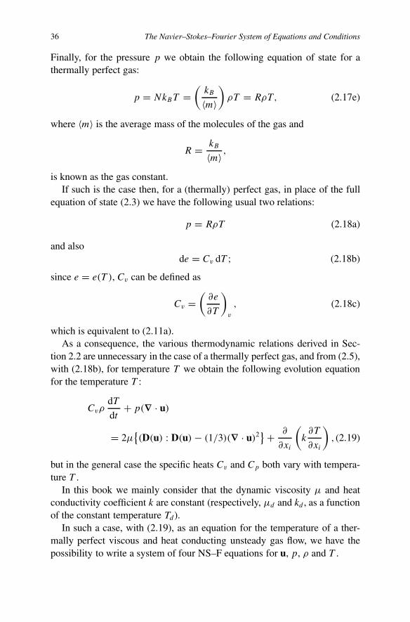
36 The Navier–Stokes–Fourier System of Equations and Conditions
Finally, for the pressure p we obtain the following equation of state for athermally perfect gas:
p = NkBT =(kB
〈m〉)ρT = RρT, (2.17e)
where 〈m〉 is the average mass of the molecules of the gas and
R = kB
〈m〉 ,
is known as the gas constant.If such is the case then, for a (thermally) perfect gas, in place of the full
equation of state (2.3) we have the following usual two relations:
p = RρT (2.18a)
and alsode = Cv dT ; (2.18b)
since e = e(T ), Cv can be defined as
Cv =(∂e
∂T
)v
, (2.18c)
which is equivalent to (2.11a).As a consequence, the various thermodynamic relations derived in Sec-
tion 2.2 are unnecessary in the case of a thermally perfect gas, and from (2.5),with (2.18b), for temperature T we obtain the following evolution equationfor the temperature T :
CvρdT
dt+ p(∇ · u)
= 2µ{(D(u) : D(u) − (1/3)(∇ · u)2
} + ∂
∂xi
(k∂T
∂xi
), (2.19)
but in the general case the specific heats Cv and Cp both vary with tempera-ture T .
In this book we mainly consider that the dynamic viscosity µ and heatconductivity coefficient k are constant (respectively, µd and kd , as a functionof the constant temperature Td).
In such a case, with (2.19), as an equation for the temperature of a ther-mally perfect viscous and heat conducting unsteady gas flow, we have thepossibility to write a system of four NS–F equations for u, p, ρ and T .

Convection in Fluids 37
Namely, we have three evolution equations for u, ρ and T :
dρ
dt+ ρ(∇ · u) = 0, (2.20)
ρdudt
+ ∇p = ρf + µd[�u + (1/3)∇(∇ · u)], (2.21)
Cv
dT
dt= −
(p
ρ
)(∇ · u)+�+
(kd
ρ
)�T , (2.22a)
with
� = 2
(µd
ρ
) {D(u) : D(u)− (1/3)(∇ · u)2
}, (2.22b)
and the usual equation of state for p:
p = RρT . (2.23)
In equation of state (2.23), R is the gas constant (= 2.870 ×103 cm2/sec2◦C for dry air) and we have Carnot’s law
Cp − Cv = R.
On the other hand the coefficient of thermal expansion for a thermally perfectgas is
α = 1
T,
and for isothermal coefficient of compressibility (see (2.16) we have
β = 1
p.
For the specific entropy, we have the explicit expression
S = Cv log(pρ−γ ), (2.24a)
which is a consequence of the thermodynamic relation (equivalent to (2.6))
T dS = dh−(
1
ρ
)dp, (2.24b)
where (h is the enthalpy)
h = e +(p
ρ
), (2.24c)

38 The Navier–Stokes–Fourier System of Equations and Conditions
which is derivable from the First Law (conservation of energy) and SecondLaw (relative to entropy) of thermodynamics.
Naturally, in real conditions, properties of common gases are dependenton T and ρ. As to examples, the reader can find these in the book by Batch-elor [2, appendix 1, pp. 594–595], some observed values of the dynamicviscosity µ, kinematic viscosity ν (= µ/ρ), thermal conductivity k, thermaldiffusivity κ (= k/ρCp) and Prandtl number Pr (= ν/κ), corresponding tovalues of temperature T and density ρ.
2.4 NS–F System for an Expansible Liquid
When the temperature of a liquid is increased, with the pressure held con-stant, the liquid (usually) expands. If the momentum flux alone contributedto the pressure, the consequent fall in density would be such as to keep ρTconstant, as in the case of a gas. But the contribution to the pressure from in-termolecular forces is more important, and has a less predictable dependenceon temperature. Of course for very (ultra) thin films the (long-range) inter-molecular interactions (forces) play an important role (taking into accountthe van der Waals attraction).
In general, measurements show rather smaller values of the coefficient ofthermal expansion α (defined as in (2.9b)) for liquids, than the value 1/Tappropriate to a thermally perfect gas, namely, for water at 15◦C,
α ≈ 1.5 × 10⁻⁴/◦C.
But values of α for other common liquids tend to be larger, and range up toabout 16 × 10−4/◦C. The value of γ (= Cp/Cv) may be taken as unity forwater at temperatures and pressures near the normal values.
Quite small changes of density correspond, at either constant temperatureor at constant entropy, to enormous changes in pressure; that is, the coef-ficient of compressibility for liquids is exceedingly small. For instance, thedensity of water increases by only 0.5% when the pressure is increased fromone to 100 atmospheres at constant (normal) temperature! This great resis-tance to compression is the important characteristic of liquid, so far as fluiddynamic is concerned, and it enables us to regard them for most purposes asbeing almost incompressible with high accuracy.
On the contrary, liquids are very sensitive to expansion under the influenceof temperature and in the case of an expansible/dilatable liquid the analysisis more subtle, concerning the derivation of an evolution equation for thetemperature T .

Convection in Fluids 39
In reality, in place of the equation of state (2.8), ρ = ρ(T , p), usuallyit is assumed that the expansible liquid can be described by the followingapproximate (truncated) law state:
ρ = ρd[1 − αd(T − Td) + χA(p − pA)], (2.25)
where (ρd, Td, pA) are some constant values for the density, temperature andpressure. In Dutton and Fichtel [3], such an approximate equation of state(2.25) has been adopted by the authors, who attempt to present in a unifiedtheory the cases of liquids and of gases. Indeed, this unification has beenrealized by Bois in [4], where this unification is presented in a more precise,rational, manner.
In (2.25) the constant coefficients, αd and χA
are, respectively:
αd = −(
1
ρd
) [∂ρ
∂T
]d
, (2.26a)
χA
=(
1
ρd
) [∂ρ
∂p
]A
, (2.26b)
where [∂ρ/∂T ]d and [∂ρ/∂p]A are both constant.From relation (2.16), with (2.26a, b), we obtain the following remarkable
relation between the constant coefficients αd and χA:
α2d
χA
= Cvd(γ − 1)
[ρd
Td
]. (2.27)
Now, with the relation (2.13b), from equation (2.7a), we obtain for our ex-pansible liquid the following evolution equation for liquid temperature T :
ρCp
dT
dt− αT
dp
dt= �+ kd�T, (2.28)
where the viscous dissipation � (per unit of mass) is given by the sameexpression (2.22b) used for a thermally perfect, viscous and heat conducting,gas.
Here, for the considered liquids, the coefficients χA
and αd are usuallyvery small (for water at 15◦C, αd ≈ 10−4/◦C) and for a bounded value of theright-hand side in relation (2.27), when χ
A↓ 0, it is necessary that α2
d/χA
remain also bounded.As a consequence we can write a similarity rule between the two small
parameters, ε = α(Td)�T , defined by (1.10a) in Chapter 1, and
� = gdρdχ(pA). (2.29)

40 The Navier–Stokes–Fourier System of Equations and Conditions
Namely:ε2 = K0 �, (2.30)
where the similarity parameter K0 is fixed – not very much large or small –when both ε and � tend to zero.
Usually, in applications, it is sufficient to assume that Cp is only a functionof temperature T , such that (see, for instance [4]):
Cp = Cpd[1 − αd�pd(T − Td)] (2.31)
where �pd = const.On the other hand, in the left-hand side of equation (2.28) for the liquid’s
temperature, the coefficient α (coupled with the term T dp/dt) is usuallyassumed to be a constant and written as αd , but in an asymptotic modellingapproach, when the expansibility parameter ε tends to zero this hypothesis isuseless.
Finally, for an expansible liquid we have, as starting full NS–F equations,for u, p, T , the following system of three (2.32a–c) evolution equations:
dρ
dt+ ρ(∇ · u) = 0, (2.32a)
ρdudt
+ ∇p = ρf + µd [�u + (1/3)∇(∇ · u)], (2.32b)
ρCp
dT
dt− αT
dp
dt= �+ kd�T, (2.32c)
with the approximate equation of state for ρ:
ρ = ρd
{1 − ε
[(T − Td)
�T
]+
(1
K0
)ε2
[(p − pA)
g dρd
]}, (2.32d)
where the coefficient Cp, in equation (2.32c), according to (2.31), is givenby the relation (the difference of temperature �T = TW − Td):
Cp = Cpd
{1 − ε�pd
[(T − Td)
�T
]}. (2.33)
2.5 Upper Free Surface Conditions
In the mathematical formulation of the full Bénard, heated from below, con-vection problem – considered in detail in the framework of Chapter 4 –

Convection in Fluids 41
Fig. 2.1 Geometry of the Bénard convection problem, heated from below.
we have in view a physical thermal problem in a layer of expansible liquidwhich is in contact with a solid heated wall (z = 0) of constant temperature,T = Tw.
This weakly expansible liquid layer is separated – from a motionless am-bient passive atmosphere at constant temperature TA and constant pressurepA, having negligible viscosity and density – by an upper (at the level z = d)free surface simulated by the following Cartesian equation (see Figure 2.1):
z = d + ah(t, x, y) ≡ H(t, x, y). (2.34)
Across the free surface given by (2.34) we assume that no mass flows isrealized and from the balance of momentum we can write the classical freesurface jump condition for the pressure fifference (p − pA). Namely,
(p − pA)n = 2µd [D(u)− (1/3)(∇ · u)] · n
− 2σ (T )Kn − ∇‖σ (T ), at z = H(t, x, y), (2.35)
according to constitutive relation (1.4a) for the stress tensor.In (2.35), the unit outward normal vector n is directed from the liquid to
the passive ambient air and the surface gradient operator ∇‖ is defined as:
∇‖ = ∇ − (n · ∇)n (2.36a)
while the mean curvature is
K = −(1/2)[∇‖ · n]. (2.36b)
We observe that in the free surface jump condition (2.35), the surface vis-cosities have been neglected. The Marangoni thermocapillary effect is di-rectly connected with the last term in the right-hand side of (2.35) and wecan write:

42 The Navier–Stokes–Fourier System of Equations and Conditions
∇‖σ (T ) =[
dσ (T )
dT
]∇‖T , (2.36c)
where according to (1.17a, b) and (1.13)
σ (T ) = σ (Td)−[−dσ (T )
dT
]d
�T θ, (2.36d)
�T = Tw−Td , when we work with the dimensionless temperature θ definedby the relation (1.13).
As balance of the temperature T , at a free surface we use, as in Chap-ter 1, the condition (1.23b), which simulates the conservation of heat flux ontransport across the upper, deformable free surface in a convection regime.This upper condition (1.23b), for the temperature T (t, x, y, z) of the liquid,at free surface z = H(t, x, y), is in fact, a so-called ‘third-mixed type’ (orRobin) condition, embracing the classical Dirichlet condition (T = TA atthe free surface, in the case of a perfectly conducting free surface) and Neu-mann condition (at the free surface ∂T /∂n = 0, for a poor conducting freesurface).
We observe that, on the contrary, in the linear (approximate) relation(1.17a)/(2.36d), for the surface tension σ (T ), we have as the difference ofthe temperature (T − Td), where the reference temperature Td is the interfa-cial temperature of the basic conduction state, i.e., the constant temperatureof the flat film z = d. On the one hand, the ‘Marangoni effect’, linked withthe temperature-dependent surface tension, is operative along the free sur-face, and, on the other hand, the ‘Biot effect’, linked with the rate of heatloss from the free surface, is operative across this free surface! Indeed, in thecase of a convection regime with a deformable upper free surface, it seemsjudicious to use for both effects (Marangoni and Biot) the difference of thetemperature [T − TA], and work with the dimensionless temperature � de-fined by (1.17c) because, in this convection regime case, the temperatureT = Td at flat film, z = d, does not have a real physical sense! Namely, wewrite in such a case for �, in place of (1.23b), that the free surface, z = H ,is cooled by air currents according to the law:
−k(Td)∂�∂n
= qconv�+ Q0
(Tw − TA), at z = H(t, x, y), (2.37)
when T = TA + (Tw − TA)�.The justification for such an upper, free-surface condition (2.37), for the
temperature of the liquid (with qconv �= qs(Td)), relies on the assumption thatheat convection, within the liquid, is so much faster than within air and the

Convection in Fluids 43
heat flux on the free surface, considered from the inside of the fluid, maybe approximated by such a difference in temperature according to Newton’scooling law!
It seems that the introduction of a second (different from conduction qs)convective heat transfer coefficient qconv, in a convection regime, when thecondition (1.23b) or (2.37) is used, is reasonable for a more rational and cor-rect formulation of the problem of Marangoni’s instability. Of course, wemake precise, again, that this rational way does not resolve the untractableheat transfer coupled, air–free surface–liquid, problem, and in particular thedetermination of the coefficient qconv (for example, as a function of the tem-perature of the liquid T or of the upper, free-surface deformation h(t, x, y))remains obviously an open problem – but, in return, the mathematical for-mulation is correct!
The discussion concerning the above upper, free-surface condition (2.37),for the dimensionless temperature �, will be complemented in Section 4.4.
Finally, the location of the deformable free surface, (2.34), z = H(t, x, y),is determined via the usual kinematic condition
d
dt[z−H(t, x, y)] = 0, on z = H(t, x, y). (2.38)
If the truth must be told, in general, the density ρ as a function of T andp, according to equation of state (2.8), must be written as
ρ = ρ(T , p) = ρd
{1 − α(Td)(T − Td)+ χ(pA)(p − pA)
+ (1/2)
[α2(Td)−
(∂α(T )
∂T
)Td
](T − Td)
2 + · · ·}, (2.39)
when an expansion in a Taylor’s series about some constant thermodynamicreference (fiducial) state (ρd, Td, pA) is performed. If we consider an idealliquid, according to the Dutton and Fichtl paper [3], then only three firstterms are taken into account in (2.39), as this is the case in Section 2.4 (see(2.25) or (2.32d)).
However, the third term, proportional to pressure difference, (p − pA), in(2.32d), is in fact a second-order term relative to small parameter ε, when wetake into account the similarity rule (2.30).
Often in thermal convection - for instance, in Bénard, heated from below,thermal convection – à la Rayleigh’s problem – considered in Chapter 3, asapproximate equation of state for an expansible liquid, the following simpli-fied, leading-order equation of state is adopted:

44 The Navier–Stokes–Fourier System of Equations and Conditions
ρ ≈ ρd{1 − α(Td)(T − Td)} ≡ ρd(1 − εθ), (2.40)
where ε = α(Td)�T , with �T = Tw − Td , which, at the leading order, isconsistent (with an error of order O(ε2)), if we take into account the relation(2.32d) which is a consequence of the similarity rule (2.30) – the dimension-less temperature, θ , being given by (1.13).
We make precise also that, for an ideal expansible liquid (when (2.25)is assumed), the coefficients α(Td) ≡ αd and χ(pA) ≡ χ
Aand also (in
(2.33)) Cp(T ) ≡ Cpd are often assumed constant over the range of variationpermitted in the fiducial states (ρd, Td, pA), this is certainly the case at theleading order (when ε ↓ 0) in an asymptotic modelling approach!
Concerning the approximate, extended, equation of state (2.39), the mainproblem concerns the influence of the fourth term, proportional to (T −Td)
2,when we want to derive a second-order approximate model. On the otherhand, the third term, χ
A(p − pA), in (2.39), rewritten for the perturbation of
the pressure π , defined by (1.26), has the following approximate form:
χA(p − pA) ≈ ε2[Fr2
dπ + 1 − z′)], (2.41)
at least when we assume that, in similarity rule (2.30), K0 is not very smallor not very large.
Now, concerning the upper, free-surface, jump condition, (2.35); this vec-torial single condition gives three boundary conditions at the free surfacez = H(t, x, y) simulated by equation (2.34).
Let t(1) and t(2) be two unit tangent vectors parallel to upper, free surfacez = H(t, x, y) given by (2.34) and both orthogonal to unit outward normalvector n to this free surface, such that
t(1) · n = 0,
andt(2) · n = 0.
In this case, in place of the single vectorial upper, free-surface, jump condi-tion (2.35), we obtain the following three scalar upper, free-surface boundaryconditions:
p = pA + µd [dij ninj − (2/3)(∇ · u)] + σ (T )(∇‖ · n), (2.42a)
µddij t(1)i nj =
[dσ (T )
dT
]t(1)i
(∂T
∂xi
), (2.42b)

Convection in Fluids 45
µddij t(2)i nj =
[dσ (T )
dT
]t(2)i
(∂T
∂xi
), (2.42c)
written at free surface z = d + ah(t, x, y) ≡ H(t, x, y), where, accordingto (1.4b),
dij = (1/2)
[∂ui
∂xj+ ∂uj
∂xi
].
We observe also that
∇‖ · n = −(
1
N3/2
) {Ny
∂2H
∂x2− 2
(∂H
∂x
) (∂H
∂y
)∂2H
∂x∂y+Nx
∂2H
∂y2
},
(2.43a)with
N = 1 +(∂H
∂x
)2
+(∂H
∂y
)2
, (2.43b)
Nx = 1 +(∂H
∂x
)2
, (2.43c)
Ny = 1 +(∂H
∂y
)2
. (2.43d)
According to Pavithran and Redeekop [5], the components (t (1)i and t (2)i ) oftwo tangential vectors, t(1) and t(2), in conditions (2.42b, c), and components(ni) of the outward unit vector, n, to the deformed upper, free surface z =H(t, x, y), are written below in terms of the (x, y, z) Cartesian system ofcoordinates. Namely we have:
t(1) =[
1
N1/2x
] (1; 0; ∂H
∂x
); (2.44a)
t(2) =[
1
N1/2x N1/2
] (−∂H
∂x
(∂H
∂y
); 1 +
(∂H
∂x
)2
; ∂H∂y
), (2.44b)
n =[
1
N1/2
] (−∂H
∂x;−∂H
∂y; 1
). (2.44c)
Obviously the convection problem, heated from below, for a liquid layerbounded above by an upper, free surface, z = H(t, x, y), in a convectiveregime is more difficult mainly because of the complexity of the above upper,free-surface conditions (2.42a–c) with (2.43a–d) and (2.44a–c).
Again, concerning the upper, free-surface condition for the temperature,if now we work with the dimensionless temperature θ , and we choose New-ton’s cooling law in the form (1.23b), as in Chapter 1, then as condition,instead of (2.37), we have (see (1.24b)):
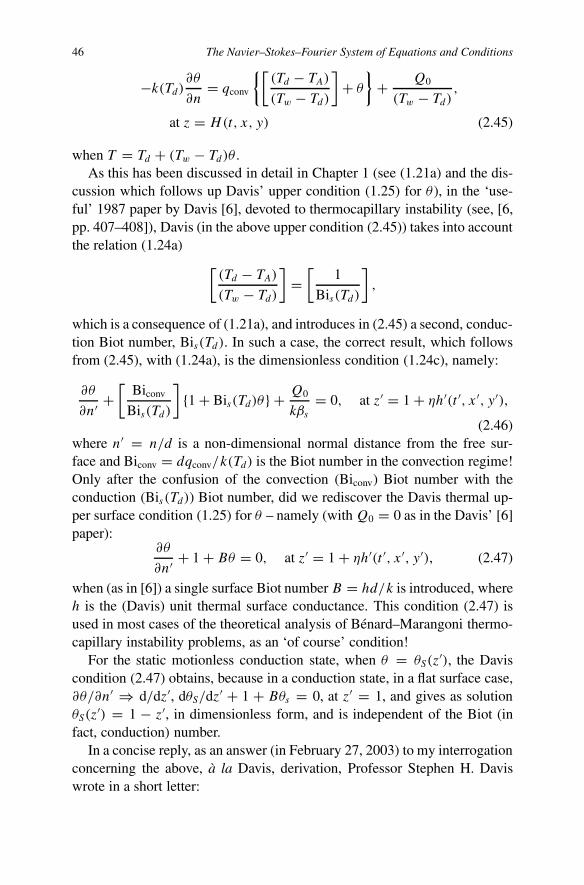
46 The Navier–Stokes–Fourier System of Equations and Conditions
−k(Td)∂θ∂n
= qconv
{[(Td − TA)
(Tw − Td)
]+ θ
}+ Q0
(Tw − Td),
at z = H(t, x, y) (2.45)
when T = Td + (Tw − Td)θ .As this has been discussed in detail in Chapter 1 (see (1.21a) and the dis-
cussion which follows up Davis’ upper condition (1.25) for θ), in the ‘use-ful’ 1987 paper by Davis [6], devoted to thermocapillary instability (see, [6,pp. 407–408]), Davis (in the above upper condition (2.45)) takes into accountthe relation (1.24a)
[(Td − TA)
(Tw − Td)
]=
[1
Bis(Td)
],
which is a consequence of (1.21a), and introduces in (2.45) a second, conduc-tion Biot number, Bis(Td). In such a case, the correct result, which followsfrom (2.45), with (1.24a), is the dimensionless condition (1.24c), namely:
∂θ
∂n′ +[
Biconv
Bis(Td)
]{1 + Bis(Td)θ} + Q0
kβs= 0, at z′ = 1 + ηh′(t ′, x′, y′),
(2.46)where n′ = n/d is a non-dimensional normal distance from the free sur-face and Biconv = dqconv/k(Td) is the Biot number in the convection regime!Only after the confusion of the convection (Biconv) Biot number with theconduction (Bis(Td)) Biot number, did we rediscover the Davis thermal up-per surface condition (1.25) for θ – namely (with Q0 = 0 as in the Davis’ [6]paper):
∂θ
∂n′ + 1 + Bθ = 0, at z′ = 1 + ηh′(t ′, x′, y′), (2.47)
when (as in [6]) a single surface Biot number B = hd/k is introduced, whereh is the (Davis) unit thermal surface conductance. This condition (2.47) isused in most cases of the theoretical analysis of Bénard–Marangoni thermo-capillary instability problems, as an ‘of course’ condition!
For the static motionless conduction state, when θ = θS(z′), the Davis
condition (2.47) obtains, because in a conduction state, in a flat surface case,∂θ/∂n′ ⇒ d/dz′, dθS/dz′ + 1 + Bθs = 0, at z′ = 1, and gives as solutionθS(z
′) = 1 − z′, in dimensionless form, and is independent of the Biot (infact, conduction) number.
In a concise reply, as an answer (in February 27, 2003) to my interrogationconcerning the above, à la Davis, derivation, Professor Stephen H. Daviswrote in a short letter:

Convection in Fluids 47
One is free to allow the heat-transfer coefficient, h, depending on a vari-ety of things involving as much complexity as one wishes. The simplestcase of constant h is satisfactory for many problems. If in a particularcase the theory diverges from the experimental results, then one has astrong case to add ‘new effects’, and I have no objection to this. Wechose the simplest case to analyze.
Unfortunately, this, ‘rather trivial’, answer has no relation to my above analy-sis, which shows that the problem is not linked with the constancy of theheat-transfer coefficient, h, in a convective regime or with any ‘divergence’of the theory from the experimental results. The main mistake in Davis’ [6]derivation, of his above condition (2.47), is mainly related with the assump-tion (in a ‘hidden manner’) that, conduction and convection heat-transfer co-efficients are identical – which is, from the physics of the thin film problem,an untenable assertion!
For an arbitrary heat-transfer coefficient in a convection regime (qconv),obviously different from the conduction heat-transfer coefficient (qs), thecorrect upper, free- surface condition for θ is the above dimensionless con-dition (2.46) when we adopt the Davis derivation way correctly!
In a paper by Scheid et al., the reader can find some remarks (see [7,pp. 241–242]) concerning the vanishing (single) Biot number case consid-ered, in particular, by Takashima in 1981 [8], in his linear theory. This van-ishing (convection) Biot number case is a special case which deserves a se-rious critical approach.
In a different approach from that performed (à la Davis) in [6]), Pear-son’s [9] theoretical treatment was based on a linear stability analysis and isdiscussed more in detail in Section 4.4. In fact, we can consider a slight ex-tension of Pearson’s approach (without any linearization) in order to obtainan upper, free-surface, boundary condition for the dimensionless temperature(see (1.17c),
�
[= (T − TA)
(Tw − TA)
]. (2.48)
Namely, from the general (see Section 4.4) upper, free-surface condition(4.46a), when for the rate of heat loss Q(T ) from the free surface we write
Q(T ) = Qs +[
dQ(T )
dT
]A
(T − TA), (2.49)
where TA is again the constant ambient motionless air temperature above theupper, free surface. As a consequence, with Qs = k(TA)βs , where here for
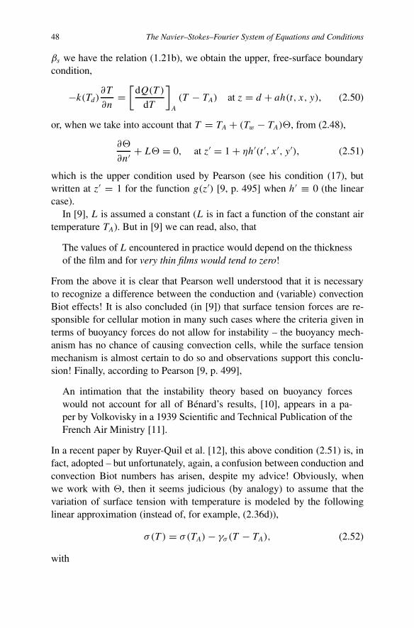
48 The Navier–Stokes–Fourier System of Equations and Conditions
βs we have the relation (1.21b), we obtain the upper, free-surface boundarycondition,
−k(Td)∂T∂n
=[
dQ(T )
dT
]A
(T − TA) at z = d + ah(t, x, y), (2.50)
or, when we take into account that T = TA + (Tw − TA)�, from (2.48),
∂�
∂n′ + L� = 0, at z′ = 1 + ηh′(t ′, x′, y′), (2.51)
which is the upper condition used by Pearson (see his condition (17), butwritten at z′ = 1 for the function g(z′) [9, p. 495] when h′ ≡ 0 (the linearcase).
In [9], L is assumed a constant (L is in fact a function of the constant airtemperature TA). But in [9] we can read, also, that
The values of L encountered in practice would depend on the thicknessof the film and for very thin films would tend to zero!
From the above it is clear that Pearson well understood that it is necessaryto recognize a difference between the conduction and (variable) convectionBiot effects! It is also concluded (in [9]) that surface tension forces are re-sponsible for cellular motion in many such cases where the criteria given interms of buoyancy forces do not allow for instability – the buoyancy mech-anism has no chance of causing convection cells, while the surface tensionmechanism is almost certain to do so and observations support this conclu-sion! Finally, according to Pearson [9, p. 499],
An intimation that the instability theory based on buoyancy forceswould not account for all of Bénard’s results, [10], appears in a pa-per by Volkovisky in a 1939 Scientific and Technical Publication of theFrench Air Ministry [11].
In a recent paper by Ruyer-Quil et al. [12], this above condition (2.51) is, infact, adopted – but unfortunately, again, a confusion between conduction andconvection Biot numbers has arisen, despite my advice! Obviously, whenwe work with �, then it seems judicious (by analogy) to assume that thevariation of surface tension with temperature is modeled by the followinglinear approximation (instead of, for example, (2.36d)),
σ (T ) = σ (TA)− γσ (T − TA), (2.52)
with

Convection in Fluids 49
γσ = −[
dσ (T )
dT
]A
. (2.53)
In Section 4.4, we again discuss this problem concerning the thermal up-per, free-surface condition, but mainly for the dimensionless temperature �,and also the dimensionless modellling of the term (2.36c) expressing thethermocapillary stress in the free-surface jump condition (2.35).
2.6 Influence of Initial Conditions and Transient Behavior
For the NS–F systems derived above (see Sections 2.3 and 2.4), consistingof three evolution equations for ui , T and p, because the partial derivativesin time t , dui/dt , dT /dt and dp/dt are present (see for instance (2.32a–c)),it is necessary to assume that three initial data at initial time u0
i , T0 and p0,
are given as functions of coordinates; namely, for t = 0, we write
at t = 0, ui = u0i , T = T 0 and p = p0, (2.54)
where T 0 and p0 are positive known data and we observe that in varioustechnological applications, often, it is essential to take into account theseabove three initial conditions (2.54).
However, in the framework of a rational analysis and asymptotic mod-elling of a weakly expansible liquid layer heated from below, our main pur-pose is the formulation (when the expansibility parameter, ε tends to zero)of leading-order, approximate, consistent models, for the considered convec-tion problem, in accordance with various values of the square of a referenceFroude, Fr2
d , number based on the thickness of the liquid layer d. Unfortu-nately, the passage from the full exact starting equations with given initialconditions and associated to convection problem boundary conditions, to alimiting approximate convection model is, in general, singular.
This singular nature is mainly expressed by the fact that: often via the lim-iting passage, some partial derivatives in time (present in full exact startingequations) disappear in derived model equations and, as a consequence, it isnot possible to apply all the given in start initial conditions at t = 0.
As a consequence, certainly, the asymptotically-derived, limiting, approx-imate model equations are not valid in the vicinity of the initial time, and ashort-time-scale, local in time, rational analysis is necessary!
In the framework of an asymptotic modelling, the logical rational wayfor solving the associated local/short-time problem is the consideration ofan initial time layer near time = 0. In this initial time layer a new, local,

50 The Navier–Stokes–Fourier System of Equations and Conditions
dimensionless, model of unsteady equations is derived where, in place ofthe non-dimensional (evolution) time t ′, a new (adjustment) short-time, τ ′, isintroduced in local equations governing the associated adjustment problem.For example, if the approximate limiting model problem (significant outsideof the singular initial time layer) is asymptotically derived via the limitingprocess
ε tends to zero, (2.55)
then the corresponding short time is
τ ′ = t ′
ε(2.56)
Often, the new, local-in time, dimensionless, model problem, with allderivatives relative to τ ′, is an unsteady linear problem with all (starting)initial conditions. This local-in time problem is an unsteady adjustment prob-lem and (matching) when τ ′ tends to infinity, we discover the initial condi-tions at t ′ = 0 for the limiting model evolution problem derived, for instance,according to (2.55).
In other words, close to initial time, τ ′ = 0, an unsteady (relative to shorttime τ ′) local problem is considered with the given starting initial conditions,and then the limiting value, when τ ′ → ∞, of the solution of this localproblem are adjusted to a set of new initial conditions at t ′ = 0 for thepreviously derived, limiting, simplified evolution model equations.
Otherwise:
lim(local when τ ′ → ∞) = lim(model at t ′ = 0). (2.57)
A typical example is considered in a paper by Dandapat and Ray [14],where the flow of a thin liquid film over a cold/hot rotating disk is analyzedfor a small Reynolds number
Re = U0h0
ν� 1; (2.58)
in this ‘low Reynolds number’ situation, the balance of centrifugical forceand the viscous shear across the film defines a characteristic time (denotedby the authors in [14] by tb):
tb = ν
(h20�
2). (2.59)
The characteristic velocity scale, U0, is defined as h0/ν, where h0 is theinitial (at time = 0) film thickness, � is angular velocity and ν the kinematic

Convection in Fluids 51
viscosity. We return to this thin liquid film problem over a cold/hot rotatingdisk in Chapter 10 of this book.
Here we observe, only, that the problem considered in [14] is, in fact, anextension of an unsteady problem considered in [15], by Higgins (and alsoin my recent book [16], section 5.4 devoted to very low Reynolds numberflows, where the main lines of the Higgins problem are exposed). In [17],Hwang and Ma studied the film thickness and its dependence on variousparameters. In the paper [14], Dandapat and Ray reconsider the problemexamined in [18] by taking into account the effect of the variation of thesurface tension with temperature (Marangoni effect) and thermal stress onthe free surface (Newton’s law of cooling is taking into account – but, infact, the heat transfer coefficient is assumed later to be 0).
The influence of initial conditions on transient thin-film flow, has beenrecently examined by Khayat and Kim [19]. This study investigates, the-oretically, the influence of initial conditions on the development of earlytransients for pressure-driven planar flow of a thin film over a stationarysubstrate, emerging from a channel. The flow is governed by the thin filmequations of boundary-layer type and the wave and flow structure are exam-ined for various initial conditions of flow and film profile. It is found that,depending on the initial film profile and velocity distribution, the limitingsteady state may or may not be reached (stable) – alternatively, the insta-bility of the steady state is shown to be closely linked to the existence of agradient catastrophe.
In various classical simplified model problems for a film and, in particular,in the case of the derivation of a lubrication equation, via the long-waveapproximation theory and, also, when an averaged integral boundary-layer(IBL) approach is used, the initial conditions must be specified for the modelevolution (in time) equations – but the number of these initial conditions forthese model equations is, usually, less than that for the full dominant startingequations? Again, this is caused by the fact that, during limiting processes,some time derivatives disappear in derived limiting model equations and,obviously, in each case, it is necessary to put the following question: whatinitial conditions can be imposed to a derived approximate model problemand how are these initial conditions related to the initial given data for fulldominant starting equations?
It is also important to note that, depending on the kind of convection prob-lems, we may have mainly two kinds of behavior, for the solution of theunsteady adjustment local-in time process, when the rescaled time goes toinfinity! Either one may have a tendency towards a limiting steady state (and

52 The Navier–Stokes–Fourier System of Equations and Conditions
in such a case the matching is ensured) or an undamped set of oscillationsappear (and it is necessary to apply a multiscale asymptotic method).
Actually, unfortunately, in RB, BM and lubrication problems and also inthe averaged integral boundary-layer, IBL, approach, the associated unsteadyadjustment model (inner) problems, valid in the vicinity of the initial time,are often not regarded or even discussed? In spite of the fact that, obviously,for many technological problems, related in particular with thin films, suchan inner/local in time approach is required for a truthful time evolution pre-diction, the transient behavior playing more often than not an important role!In Section 10.8 of we give an interesting, singular, example where a match-ing is realized.
2.7 The Hills and Roberts’ (1990) Approach
Hills and Roberts [20] – see the book by Straughan [21, pp. 48–49]) – forthe full system of equations (1.1a–c) consider, first, the entropy productioninequality
ρ
[T S − de
dt
]+ Tjidji −
(qiT
) [∂T
∂xi
]≥ 0. (2.60)
Their interest is in liquids whose density ρ can be changed mainly by varia-tions in the temperature T , but not in the thermodynamic pressure P (whenthe Stokes relation is not taken into account), so they formulate the constitu-tive theory in terms of P and T . They argue that the natural thermodynamicpotential is the Gibbs energy:
G = e − ST + P
ρ(2.61)
and (2.60) may thus rewritten as
−ρ(
dG
dt+ S
dT
dt
)+ dP
dt+ (Tji + Pδji)dij −
(qiT
)[∂T
∂xi
]≥ 0. (2.62)
Namely, as constitutive theory, according to Hills and Roberts’ paper [20],we have
G = G(T, P ), S = S(T , P ), ρ = ρ(T ), (2.63)
Tij = −pδij + λdmmδij + 2µdij , (2.64)
qi = −k ∂T∂xi
, (2.65)

Convection in Fluids 53
where p is the mechanical pressure, and the two coefficients, λ and µ, of theviscosity and coefficients k of the thermal conductivity depend on P and T .
For the form of ρ in (2.63), the continuity equation becomes (since χ ≡ 0)as usually:
∂ui
∂xi= α
dT
dtwith α = −
(1
ρ
)dρ
dt, (2.66)
which is regarded as a constraint and then included in (2.62) via a Lagrangemultiplier �. By using the arbitrariness of the body force (and eventuallyheat supply, ρr, in the third equation (1.1c) of the system of equations (1.1a–c) governing the continuum regime) Hills and Roberts deduce from (2.62)that
S = −[
dG
dT+ �α
ρ
], (2.67a)
dG
dP=
(1
ρ
), (2.67b)
p = P +�, � = �(T, P ), (2.67c)
λ+ (2/3)µ ≥ 0, µ ≥ 0, k ≥ 0. (2.67d)
They then work with another modified Gibbs energy:
G∗ = G+(�
ρ
), (2.68)
which allows them to replace G, P , � by G∗, p, for which:
G∗ = G∗(T , p) = G0(T )+(p
ρ
); (2.69a)
∂G∗
∂T= −S; (2.69b)
∂G∗
∂p=
(1
ρ
), (2.69c)
where now the liquid parameters depend on mechanical pressure p and ab-solute temperature T .
The governing equations for the expansible liquid (with ρ = ρ(T ), butalso with (2.69a–c)) become in such a case,
αdT
dt= ∂ui
∂xi; (2.70a)

54 The Navier–Stokes–Fourier System of Equations and Conditions
ρdui
dt= ρfi − ∂p
∂xi
+ ∂
∂xj
[λdmmδij + 2µdij ]; (2.70b)
−αTdp
dt+ Cp
(ρ
α
) ∂ui
∂xi
= (λdii)2 + 2µdij dij + ∂
∂xi
[k∂T
∂xi
], (2.70c)
where Cp = T (∂S/∂T )p is again the specific heat at constant pressure inequation (2.70c), which is an evolution equation for the pressure p.
The system (2.70a–c) is slightly more general than our system (2.32a–c),derived in Section 4.4, because the Stokes relation (λ = −(2/3)µ) is notassumed.
References
1. J. Serrin, Mathematical principles of classical fluid mechanics. In Handbuch der Physik,Vol. WIII/1, S. Flügge (Ed.). Springer, Berlin, pp. 125–263, 1959.
2. G.K. Batchelor, An Introduction to Fluid Dynamics. Cambridge University Press, Cam-bridge, 1988.
3. J.A. Dutton and G.H. Fichtl, J. Atmosph. Sci. 26, 241, 1969.4. P.-A. Bois, Geophys. Astrophys. Fluid Dynam. 58, 45–55, 1991.5. S. Pavithran and L.G. Redeekopp, Stud. Appl. Math. 93, 209, 1994.6. S.H. Davis, Ann. Rev. Fluid Mech. 19, 403–435, 1987.7. B. Scheid, C. Ruyer-Quil, S. Kalliadasis, M.G. Velarde and R.Kh. Zeytounian, Thermo-
capillary long waves in a liquid film flow. Part 2. Linear stability and nonlinear waves. J.Fluid Mech. 538, 223–244, 2005.
8. M. Takashima, J. Phys. Soc. Japan 50(8), 2745–2750 and 2751–2756, 1981.9. J.R.A. Pearson, J. Fluid Mech. 4, 489–500, 1958.
10. H. Bénard, Revue Gén. Sci. Pures Appl. 11, 1261–1271 and 1309–1328, 1900. See alsoAnn. Chim. Phys. 23, 62–144, 1901.
11. V. Volkovisky, Publ. Sci. Tech., Ministère de l’Air 151, 1939.12. C. Ruyer-Quil, B. Scheid, S. Kalliadasis, M.G. Velarde and R.Kh. Zeytounian, Thermo-
capillary long waves in a liquid film flow. Part 1. Low-dimensional formulation. J. FluidMech. 538, 199–222, 2005.
13. M. Van Dyke, Perturbation Methods in Fluid Mechanics. Academic Press, New York,1964.
14. B.S. Dandapat and P.C. Ray, Int. J. Non-Linear Mech. 28(5), 489–501, 1993.15. B.G. Higgins, Phys. Fluids 29, 3522, 1986.16. R.Kh. Zeytounian, Theory and Applications of Viscous Fluid Flows, Springer-Verlag,
Berlin/Heidelberg, 2004.17. J.H. Hwang and F. Ma, J. Appl. Phys. 66, 388, 1989.18. B.S. Dandapat and P.C. Ray, Int. J. Non-Linear Mech. 25, 589–501, 1990.19. R.E. Khayat and K.-T. Kim, Phys. Fluids 14(12), 4448–4451, 2002.20. R. Hills and P. Roberts, Stab. Appl. Anal. Continuous Media 1, 205–212, 1991.21. B. Straughan, Mathematical Aspects of Penetrative Convection. Longman, 1993.

Chapter 3The Simple Rayleigh (1916) ThermalConvection Problem
3.1 Introduction
Lord Rayleigh, in his December 1916, pioneering paper [1] devoted to ‘OnConvection Currents in a Horizontal Layer of Fluid, when the Higher Tem-perature is on the Under Side’ first wrote
The present paper is an attempt to examine how far the interesting re-sults obtained during the years 1900–19001 by Bénard [2] in his carefuland skilful experiments can be explained theoretically. Bénard workedwith very thin layers, only about 1 mm. deep, standing on a levelledmetallic plate which was maintained at a uniform temperature. The up-per surface was usually free, and being in contact with the air was at alower temperature. Various liquids were employed.
The layer rapidly resolves itself into a number of cells, the motionbeing an ascension at the middle of a cell and a descension at the com-mon boundary between a cell and its neighbours.
And also
M. Bénard does not appear to be acquainted with James Thomson’spaper ‘On a changing Tesselated Structure in certain Liquids’ (Proc.Glasgow Phil. Soc. 1881–1882), where a like structure is described inmuch thicker layers of soapy water cooling from the surface.
In Lord Rayleigh’s paper the calculations are based upon approximate equa-tions formulated by Boussinesq in his 1903 book [3] – the special limitationwhich characterizes these so-called ‘Boussinesq equations’ is the neglect ofvariation of density, except in so far as they modify the action of gravity.According to Lord Rayleigh: ‘Of course, such neglect can be justified only
55

56 The Simple Rayleigh (1916) Thermal Convection Problem
Fig. 3.1 Geometry of the Rayleigh simple convection problem.
under certain conditions, which Boussinesq has discussed’. In Zeytounian’s2003 paper [4], a hundred years later, the reader can find a rational/logicaljustification of this Boussinesq approximation and associated Boussinesqequations; the main lines of such a justification are presented briefly below.
In fact, the present chapter is an extended version of a paper written in2006 for the 90 years of the above-mentioned Rayleigh’s pioneering 1916paper devoted to thermal convection, but . . . unpublished, for various rea-sons!
As equation of state in [1], Lord Rayleigh assumed, in fact, that
ρ = ρ(T ), (3.1a)
and in such a case
−(
1
ρ
)dρ
dT= α(T ), (3.1b)
where α(T ) is the usual coefficient of volume/thermal expansion.Lord Rayleigh [1] considered a particular, simple, ‘Rayleigh Problem’,
when the fluid is supposed to be bounded by two infinite fixed planes, re-spectively, at z = 0 and z = d, where also the temperatures (respectively, Twand Td ) are both maintained constant (see Figure 3.1).
In the case of this Rayleigh problem, we have a simple static, motionlessconduction temperature state Ts(z), such that
−dT s(z)
dz≡ βs = (Tw − Td)
d≡ �T
d, T > 0, (3.1c)
when the higher temperature Tw is below (at z = 0) and Ts(z = d) = Td .However, a little unexpectedly, it appears that the equilibrium may be thor-
oughly stable, if the coefficients of conductivity and viscosity are not toosmall – as the temperature gradient βs = (Tw − Td)/d increases, and whenβs = �T/d exceeds a certain critical value βsC (that is, when βs just ex-ceeds βsC) instability enters which produces a permanent regime of regular

Convection in Fluids 57
Fig. 3.2 Bénard cells in spermaceti. Reprinted with kind permission from [5].
hexagons – then these cells become equal and regular and align themselves(see, for instance Figure 3.2, which is a reproduction of one of Bénard’searly photographs, from [5]). Because Lord Rayleigh [1] considered a liquidlayer with a constant thickness d, the Marangoni and Biot effects are absentin the exact formulation of the thermal convection problem; the effect ofthe (constant) surface tension is also absent and the Weber number does notappear in the Rayleigh formulation of the problem. As a consequence theanalytical problem considered by Rayleigh has no relation with the physi-cal experimental problem considered by Bénard in his various experiments[2] – in Rayleigh’s simple analytical problem the main driving force, whichgives a bifurcation from a conduction motionless regime to convective mo-tion, is the buoyancy (Achimedean) force. Nevertheless, Rayleigh’s theoret-ical problem, leading to the famous ‘Rayleigh–Bénard instability problem’,is a typical problem in hydrodynamic instability and represents a transitionto turbulence in a fluid system. In my recent book [6], the reader can findvarious aspects of this RB problem with recent references – here, in thischapter, our main purpose is to give a rational/asymptotic justification of thederivation of the RB model problem and show how it is possible to improvethis leading-order RB model by a second-order consistent model which takesinto account various non-Boussinesq effects!
Now we see that temperature-dependent surface tension forces, onthe deformable free surface above a liquid layer, are sufficient to cause(Marangoni) instability and are responsible for many of the cellular patternsthat have been observed in cooling fluid layers, with at least a free surface.In such a case, the driving force for this thermocapillary convective mo-tion is provided by the flow of heat from the heated lower surface to the

58 The Simple Rayleigh (1916) Thermal Convection Problem
cooled upper, free surface. Obviously, in the case of the simple Rayleighmodel problem, considered in the present chapter, the thermocapillary con-vective (Marangoni effect) is completely absent. Concerning the Bénard ex-periments, the reader can find in Chandrasekhar’s book [5, §18] the followingshort description:
Bénard carried out his experiments on very thin layers of fluid, about amillimetre in depth, or less, standing on a levelled metallic plane main-tained at a constant temperature. The upper surface was usually free andbeing in contact with the air was at a lower temperature. He was partic-ularly interested in the role of viscosity; and as liquid of high viscosityhe used melted spermaceti and paraffin. In all cases, Bénard found thatwhen the temperature of the lower surface was gradually increased, ata cerain instant, the layer became reticulated and revealed its dissectioninto cells. He further noticed that there were motions inside the cells:of ascension at the centre, and of descension at the boundaries with theadjoining cells.
Bénard distinguished two phases in the succeeding development ofcellular pattern: an initial phase of short duration in which the cellsacquire a moderate degree of regularity and become convex polygonswith four to seven sides and vertical walls; and a second phase of rel-ative permanence in which the cells all become equal, hexagonal, andproperly aligned.
In 1993, Koschmieder, who has been for decades a key figure in the exper-imental investigation of the Bénard problem, wrote a very valuable mono-graph [7] concerning the Bénard cells (and also Taylor vortices) and thereader can find in there many figures which are results of the Koschmiederexperiences.
Although Bénard was aware of the role of surface tension and especiallyof the surface tension gradients (in particular in the case of a temperature-dependent surface tension) in his experiments, it took more than five decadesto unambiguously assess, experimentally and theoretically (see for instancepapers by Block [8] and Pearson [9]), that: ‘Indeed the surface tension gradi-ents rather than buoyancy was the main cause of Bénard cells in thin (weaklyexpansible) liquid films’.
Only in 1997 was this almost evident physical fact (see the book by Guyonet al. [10, pp. 459–462]) proved rigorously, through an asymptotic approach,in [11, 12] where is formulated an ‘alternative’ that is valid in an asymptoticsignificance in leading order:

Convection in Fluids 59
Either the buoyancy is taken into account and in this case the free sur-face deformation effect is negligible and we have the possibility to takeinto account in the Rayleigh–Bénard model problem the Marangonieffect only partially or, the free surface deformation effect is takeninto account and, in such a case, the buoyancy does not play a signif-icant leading-order role in the Bénard–Marangoni full thermocapillarymodel problem.
Thanks to the above ‘alternative’ it has been possible to obtain various cri-teria for the validity of the leading order, Rayleigh–Bénard (RB), Bénard–Marangoni (BM), and Deep Convection (DB), model problems (see, for in-stance Chapter 8). These criteria have been derived thanks to our rationalanalysis and asymptotic approach, via different similarity rules.
Although Bénard initially assumed that surface tension at the free surfaceof the film was an important factor in cell formation, this idea was aban-doned for some time as the result of the work of Rayleigh in 1916 [1] wherehe analyzed the buoyancy driven natural thermal convection of a layer offluid heated from below. He found that if hexagonal cells formed, the ratioof the spacing to cell depth almost exactly equaled that measured by Bé-nard, an agreement which we now know to have been fortuitous! Rayleighshowed also that if the cells are to form, then the vertical adverse tempera-ture gradient βs = �T/d, according to (3.1c), must be sufficiently large thata particular dimensionless parameter proportional to the magnitude of thegradient exceeds a critical value – we now call this parameter the Rayleighnumber, Ra, defined in Chapter 1 by (1.9b), and rewritten here as
Ra = α(Td)βsgd4
νdκd,
when we take into account (3.1c). This Rayleigh number is a characteris-tic ratio of the destabilizing effect of buoyancy to the stabilizing effects ofdiffusion and dissipation.
It was the experimental work (in 1956) of Block [8], cited above, whichput to rest the confusion surrounding the interpretation of Bénard’s experi-ments, and which demonstrated conclusively that Bénard’s results were not aconsequence of buoyancy but were (temperature-dependent) surface tensioninduced. Among other things, he showed that cellular convection took placefor Rayleigh numbers more than an order of magnitude smaller than requiredby the Rayleigh theory.
Most importantly, if the cells are buoyancy induced, then if the thin filmis cooled from below the density gradient and gravity will be in the samedirection and the film will be stably stratified.
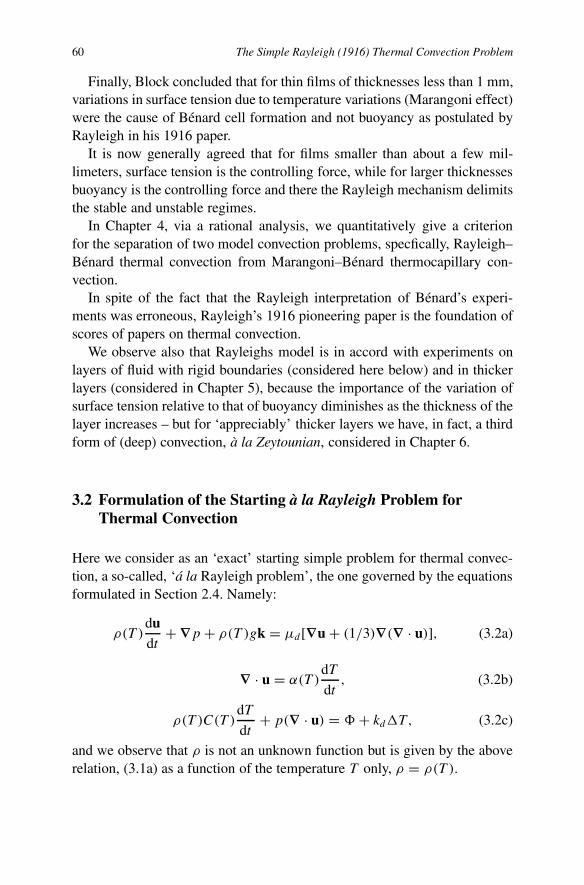
60 The Simple Rayleigh (1916) Thermal Convection Problem
Finally, Block concluded that for thin films of thicknesses less than 1 mm,variations in surface tension due to temperature variations (Marangoni effect)were the cause of Bénard cell formation and not buoyancy as postulated byRayleigh in his 1916 paper.
It is now generally agreed that for films smaller than about a few mil-limeters, surface tension is the controlling force, while for larger thicknessesbuoyancy is the controlling force and there the Rayleigh mechanism delimitsthe stable and unstable regimes.
In Chapter 4, via a rational analysis, we quantitatively give a criterionfor the separation of two model convection problems, specfically, Rayleigh–Bénard thermal convection from Marangoni–Bénard thermocapillary con-vection.
In spite of the fact that the Rayleigh interpretation of Bénard’s experi-ments was erroneous, Rayleigh’s 1916 pioneering paper is the foundation ofscores of papers on thermal convection.
We observe also that Rayleighs model is in accord with experiments onlayers of fluid with rigid boundaries (considered here below) and in thickerlayers (considered in Chapter 5), because the importance of the variation ofsurface tension relative to that of buoyancy diminishes as the thickness of thelayer increases – but for ‘appreciably’ thicker layers we have, in fact, a thirdform of (deep) convection, à la Zeytounian, considered in Chapter 6.
3.2 Formulation of the Starting à la Rayleigh Problem forThermal Convection
Here we consider as an ‘exact’ starting simple problem for thermal convec-tion, a so-called, ‘á la Rayleigh problem’, the one governed by the equationsformulated in Section 2.4. Namely:
ρ(T )dudt
+ ∇p + ρ(T )gk = µd [∇u + (1/3)∇(∇ · u)], (3.2a)
∇ · u = α(T )dT
dt, (3.2b)
ρ(T )C(T )dT
dt+ p(∇ · u) = �+ kd�T, (3.2c)
and we observe that ρ is not an unknown function but is given by the aboverelation, (3.1a) as a function of the temperature T only, ρ = ρ(T ).
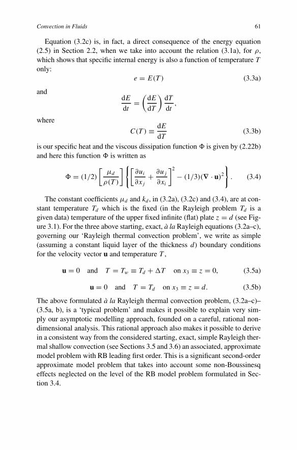
Convection in Fluids 61
Equation (3.2c) is, in fact, a direct consequence of the energy equation(2.5) in Section 2.2, when we take into account the relation (3.1a), for ρ,which shows that specific internal energy is also a function of temperature Tonly:
e = E(T ) (3.3a)
anddE
dt=
(dE
dT
)dT
dt,
where
C(T ) ≡ dE
dT(3.3b)
is our specific heat and the viscous dissipation function � is given by (2.22b)and here this function � is written as
� = (1/2)
[µd
ρ(T )
] {[∂ui
∂xj+ ∂uj
∂xi
]2
− (1/3)(∇ · u)2
}. (3.4)
The constant coefficients µd and kd , in (3.2a), (3.2c) and (3.4), are at con-stant temperature Td which is the fixed (in the Rayleigh problem Td is agiven data) temperature of the upper fixed infinite (flat) plate z = d (see Fig-ure 3.1). For the three above starting, exact, à la Rayleigh equations (3.2a–c),governing our ‘Rayleigh thermal convection problem’, we write as simple(assuming a constant liquid layer of the thickness d) boundary conditionsfor the velocity vector u and temperature T ,
u = 0 and T = Tw ≡ Td +�T on x3 ≡ z = 0, (3.5a)
u = 0 and T = Td on x3 ≡ z = d. (3.5b)
The above formulated à la Rayleigh thermal convection problem, (3.2a–c)–(3.5a, b), is a ‘typical problem’ and makes it possible to explain very sim-ply our asymptotic modelling approach, founded on a careful, rational non-dimensional analysis. This rational approach also makes it possible to derivein a consistent way from the considered starting, exact, simple Rayleigh ther-mal shallow convection (see Sections 3.5 and 3.6) an associated, approximatemodel problem with RB leading first order. This is a significant second-orderapproximate model problem that takes into account some non-Boussinesqeffects neglected on the level of the RB model problem formulated in Sec-tion 3.4.

62 The Simple Rayleigh (1916) Thermal Convection Problem
3.3 Dimensionless Dominant Rayleigh Problem and theBoussinesq Limiting Process
A dominant dimensionless form of the above Rayleigh, starting, thermal con-vection problem, (3.2a–c)–(3.5a, b), is derived when we use, at first, the non-dimensional quantities (denoted by a prime); this non-dimensionalization isa twice necessary first step in the rational approach given below. Namely, wewrite:
(x′, y′, z′) =(x1
d,x2
d,x3
d
); t ′ = t
(d2/νd); νd = µd
ρd; (3.6a)
u′i = ui
(νd/d), ∇′ = d∇; �′ = d2�; (3.6b)
π =(
1
Fr2d
){[(p − pd)
gdρd
]+ z′ − 1
}; (3.6c)
θ = (T − T d)
�T, (3.6d)
where π (unlike (1.25) because the upper surface is here the solid flat planez′ = d) and θ (as in (1.13)), are respectively, dimensionless pressure pertur-bation (when z′ = 1, then p = pd ) and dimensionless temperature reckonedfrom the temperature/point where T = Td .
We observe from the above relation (3.6d) for π that in dimensionlessform the pressure is reckoned from the point where p = pd and is related, infact, to the reference pressure ρd(νd/d)2 which is � gdρd , when we assumethat Fr2
d = (νd/d)2/gd � 1, which is just the case of a thermal convection,
where the main driving force is the buoyancy and the Boussinesq limitingprocess (3.22) is considered. Now with an error of ε2, where the expansibityparameter (defined in Chapter 1 by (1.10a)):
ε = α(Td)�T, (3.7)
is our main small parameter, we can write the following approximate,leading-order equation of state (instead of ρ = ρ(T )),
ρ(T ) = ρ(Td +�T θ) ≈ ρd[1 − εθ]. (3.8)
On the other hand, in a system of the starting equations (3.2a–c), with ρ(T ),we have also two other functions of the temperature T , α(T ) and C(T ). Byanalogy with (3.8) we write

Convection in Fluids 63
α(T ) = αd[1 − εAdθ], (3.9a)
andC(T ) = Cd[1 − ε�dθ], (3.9b)
where, respectively,
�d =[(d logC/dT )
(d log ρ/dT )
]d
(3.10a)
Ad =[(d log α/dT )
(d log ρ/dT )
]d
. (3.10b)
It seems judicious (and reasonable), if we have the ambition to derive asecond-order [with the terms proportional to ε (see Section 3.5)] thermalconvection model problem, associated with the classical/leading-order RBshallow thermal convection model problem (formulated in Section 3.4) toassume that the coefficients �d and Ad , in (3.10a, b), are both not very smallor not very large (in fact, we presuppose that �d and Ad are both ≈ 1). Inthe framework of an asymptotic theory with first-order (RB model problem)and second-order (model problem with non-Boussinesq effects) approximateproblems (instead of the full exact, starting, thermal convection problem,(3.2a–c)–(3.5a, b)), it seems that this is a very rational approach.
Now, with the above results, (3.8), (3.9a, b), and (3.10a, b), we can rewritethe vectorial equation (3.2a), of convection motion, for u′, in the followingdimensionless form, when we use the dimensionless quantities (3.6a–d).
[1 − εθ]du′
dt ′+ ∇′π − Grθ = ∇′u′ + (1/3)∇′(∇′ · u′), (3.11)
where the Grashof number, Gr, according to (1.12), is the ratio of the twosmall parameters, namely, the expansibility parameter, ε = α(Td)�T , to thesquared Froude number Fr2
d = (νd/d)2/gd:
Gr = ε
Fr2d
≡ gα(Td)d3�T
ν2d
. (3.12)
This Grashof number (3.12), defined from a fluid dynamical point of view,is directly responsible for taking account of the buoyancy effect – the maindriving, Archimedean, force in thermal convection – and, because ε � 1, itis also necessary to assume that Fr2
d � 1. Associated to the Grashof number(3.12), the Rayleigh number is defined as (see (1.9b))
Ra = gα(Td)d�T
νdκd≡ PrGr (3.13a)
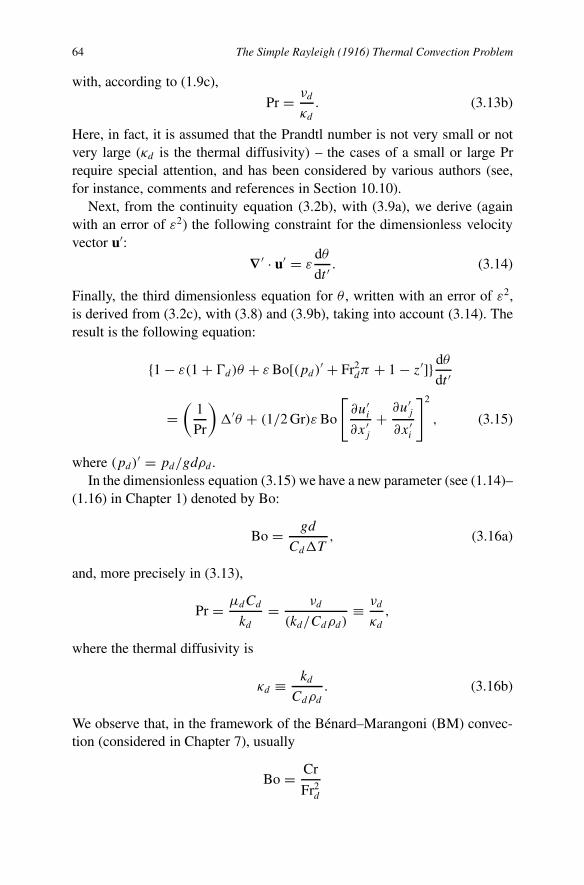
64 The Simple Rayleigh (1916) Thermal Convection Problem
with, according to (1.9c),
Pr = νd
κd. (3.13b)
Here, in fact, it is assumed that the Prandtl number is not very small or notvery large (κd is the thermal diffusivity) – the cases of a small or large Prrequire special attention, and has been considered by various authors (see,for instance, comments and references in Section 10.10).
Next, from the continuity equation (3.2b), with (3.9a), we derive (againwith an error of ε2) the following constraint for the dimensionless velocityvector u′:
∇′ · u′ = εdθ
dt ′. (3.14)
Finally, the third dimensionless equation for θ , written with an error of ε2,is derived from (3.2c), with (3.8) and (3.9b), taking into account (3.14). Theresult is the following equation:
{1 − ε(1 + �d)θ + εBo[(pd)′ + Fr2dπ + 1 − z′]} dθ
dt ′
=(
1
Pr
)�′θ + (1/2 Gr)εBo
[∂u′
i
∂x′j
+ ∂u′j
∂x′i
]2
, (3.15)
where (pd)′ = pd/gdρd .In the dimensionless equation (3.15) we have a new parameter (see (1.14)–
(1.16) in Chapter 1) denoted by Bo:
Bo = gd
Cd�T, (3.16a)
and, more precisely in (3.13),
Pr = µdCd
kd= νd
(kd/Cdρd)≡ νd
κd,
where the thermal diffusivity is
κd ≡ kd
Cdρd. (3.16b)
We observe that, in the framework of the Bénard–Marangoni (BM) convec-tion (considered in Chapter 7), usually
Bo = Cr
Fr2d

Convection in Fluids 65
is the classical Bond number which is related to the Weber, We (≡ 1/Cr),number defined by (1.18a), the parameter Cr (= 1/We) being the crispa-tion/capillary number. As in the present book we do not make use of theBond, Bo, number; our notation Bo, as a ratio of two lengths, d andCd�T/g,a number similar to a Boussinesq number (used in derivation of the Boussi-nesq approximate equations for the various meso or local atmospheric mo-tions, see Chapter 9), seems not to introduce any confusion!
The dimensionless equation (3.15), for the dimensionless temperature θ ,shows explicitly the role of the dissipation number Di∗, defined by (1.14)with (1.15) – namely:
Di∗ = (1/2)
[εBo
Gr
]≡ (1/2)BoFr2
d = (ν/d)2
2Cd�T, (3.17)
as a measure for the viscous dissipation. If we assume that Di∗ ≈ 1, then weobtain the following estimation for the thickness of the liquid film
d ≈ νd
[2Cd�T ]1/2. (3.18)
The conditionDi∗ ≈ 1, (3.18a)
which allows us, in the thermal convection model problem, to take into ac-count the viscous dissipation, leads also to the following relation for the dif-ference of the temperature �T = Tw − Td :
�T ≈ (ν/d)2
2Cd
. (3.19)
For the above dimensionless dominant equations (3.11), (3.14) and (3.15),for u′, π and θ we have from (3.5a, b) the following dimensionless boundaryconditions:
u′ = 0 and θ = 1 on z′ = 0; (3.20a)
u′ = 0 and θ = 0 on z′ = 1. (3.20b)
As a conclusion, we also observe that for the motionless conduction temper-ature Ts(z) = Tw − βsz, as a conduction dimensionless temperature θs(z),associated with θ , we have
θs(z) = [Tw − dβsz′ − Td]
(Tw − Td)=
[1 −
(dβs
�T
)z′
],
or, according to relation (1.19c) for βs ,
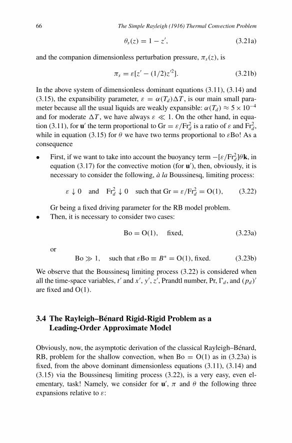
66 The Simple Rayleigh (1916) Thermal Convection Problem
θs(z) = 1 − z′, (3.21a)
and the companion dimensionless perturbation pressure, πs(z), is
πs = ε[z′ − (1/2)z′2]. (3.21b)
In the above system of dimensionless dominant equations (3.11), (3.14) and(3.15), the expansibility parameter, ε = α(Td)�T , is our main small para-meter because all the usual liquids are weakly expansible: α(Td) ≈ 5×10⁻⁴
and for moderate �T , we have always ε � 1. On the other hand, in equa-tion (3.11), for u′ the term proportional to Gr = ε/Fr2
d is a ratio of ε and Fr2d ,
while in equation (3.15) for θ we have two terms proportional to εBo! As aconsequence
• First, if we want to take into account the buoyancy term −[ε/Fr2d]θk, in
equation (3.17) for the convective motion (for u′), then, obviously, it isnecessary to consider the following, à la Boussinesq, limiting process:
ε ↓ 0 and Fr2d ↓ 0 such that Gr = ε/Fr2
d = O(1), (3.22)
Gr being a fixed driving parameter for the RB model problem.• Then, it is necessary to consider two cases:
Bo = O(1), fixed, (3.23a)
orBo � 1, such that εBo ≡ B∗ = O(1), fixed. (3.23b)
We observe that the Boussinesq limiting process (3.22) is considered whenall the time-space variables, t ′ and x′, y′, z′, Prandtl number, Pr, �d , and (pd)′are fixed and O(1).
3.4 The Rayleigh–Bénard Rigid-Rigid Problem as aLeading-Order Approximate Model
Obviously, now, the asymptotic derivation of the classical Rayleigh–Bénard,RB, problem for the shallow convection, when Bo = O(1) as in (3.23a) isfixed, from the above dominant dimensionless equations (3.11), (3.14) and(3.15) via the Boussinesq limiting process (3.22), is a very easy, even el-ementary, task! Namely, we consider for u′, π and θ the following threeexpansions relative to ε:

Convection in Fluids 67
u′ = uRB+εu1+· · · , θ = θRB+εθ1+· · · , π = πRB+επ1+· · · . (3.24)
As a leading-order result we derive, from the dominant Rayleigh equations(3.11), (3.14), (3.15), via the Boussinesq limiting process (3.22), associatedwith the three asymptotic expansions (3.24), under the constraint (3.23a), thefollowing Boussinesq, shallow convection, RB model, leading-order equa-tions:
duRB
dt ′+ ∇′πRB − Gr θRBk = �′uRB, (3.25a)
∇′ · uRB = 0, (3.25b)
dθRB
dt ′=
(1
Pr
)�′θRB. (3.25c)
As boundary conditions for these above RB model equations (3.25a–c) wewrite, according to (3.20):
uRB = 0 and θRB = 1 on z′ = 0; uRB = 0 and θRB = 0 on z′ = 1.(3.25d)
With (3.21a, b) it is possible to write the above RB model equations(3.25a–c) in a more usual form. Namely, for this we introduce, instead ofuRB, πRB and θRB, the following three new functions:
USh = Pr uRB, (3.26a)
�Sh = z′ − 1 + θRB, (3.26b)
�Sh = Gr z′[(z′/2)− 1] + πRB. (3.26c)
As a result, with the new functions (3.26a–c), instead of the equations(3.25a–c), we derive the following shallow convection – RB – equations forUSh, �Sh, �Sh:
dUSh
dt ′+ Pr ∇′�Sh − Ra�Shk = �′USh, (3.27a)
∇′ · USh = 0, (3.27b)
Prd�Sh
dt ′−WSh = �′�Sh. (3.27c)
where WSh = USh · k is the vertical component of the velocity USh in thedirection of z′, and Ra = Pr Gr is the Rayleigh number defined by (3.13a).These equations (3.27a–c) with the homogeneous boundary conditions:
USh = �Sh = 0 at z′ = 0 and z′ = 1, (3.27d)

68 The Simple Rayleigh (1916) Thermal Convection Problem
govern the rigid-rigid RB problem.Thus, we recover the classical RB, shallow, thermal convection model
rigid-rigid problem, (3.27a–d), which is usually derived in an ad hoc manner– see, for example the useful books by Drazin and Reid [13] and by Chan-drasekhar [5].
Usually, in classical hydrodynamic instability theory, a linearized ap-proach is chosen. Because, for the above rigid-rigid RB shallow thermalconvection model problem (3.27a–d), the basic motionless conduction stateis characterized by the following ‘zero’ solution:
USh = �Sh = �Sh = 0, (3.28)
then, in the case of an usual linearization when dUSh/dt ′ and d�Sh/ dt ′ arereplaced in (3.27a) and (3.27c), respectively, by ∂ULSh/∂t ′ and ∂�LSh/∂t ′,we derive a single linear equation for the ‘vertical’ – relative to z′ – compo-nent of the velocity ULSh,
ULSh · k = WLSh(z′)f (x′, y′) exp[σ t ′]. (3.29)
Namely, after some simple manipulations we obtain for WLSh(z′) the follow-
ing linear differential equation in z′:
D2(D2 − σ )(D2 − σ Pr)WLSh(z′) = −a2 Ra WLSh(z
′), (3.30a)
with∂2f
∂x′2 + ∂2f
∂y′2 + a2f = 0, (3.30b)
where a is the wave number and D2 = [d2/dz′2 − a2].The relevant boundary conditions, for the rigid-rigid, linear RB problem,
for the function WLSh(z′), solution of the linear equation (3.30a), at the rigid
flat surfaces z′ = 0 and z′ = 1, are:
WLSh(z′) = 0, (3.30c)
dWLSh(z′)
dz′ = 0, (3.30d)
D2(D2 − σ )WLSh(z′) = 0, (3.30e)
Linear equation (3.30a) for WLSh(z′) with the boundary conditions (3.30c–e)
determines a so-called ‘self-adjoint eigenvalue problem’ for the parametersRa, a2 and σ , when Pr is fixed.

Convection in Fluids 69
First, it can be proven that:
When Ra is less than a certain critical value Rac, all small disturbancesof the purely conductive basic motionless equilibrium (conduction) statedecay in time (stability). Whereas, if Ra exceeds the critical value Rac,instability occurs in the form of a convection in cells of a polygonal platform.
These cells are called Bénard cells, discovered in 1900 thanks to his quan-titative experiments (in [5, sec. 18], the reader can find an account of someof the experimental work, up to 1960, on the onset of thermal instabilityin fluids). The formation of Bénard cells in a weakly expansible liquidlayer is one of the most remarkable examples of bifucation phenomena (thebifurcations in dissipative, dynamical systems, are, in particular, investigatedin [14, chapter 10]. We observe that:
From a physical viewpoint, the fundamental process involved in RB in-stability is the transformation of the potential energy of the convectivedisturbance.
Here, we note only that, in 1940, Pellew and Southwell [15] made a compre-hensive study of linearized Bénard convection, and they conclusively proved(principle of the exchange of stabilities) that when the basic conduction tem-perature decreases upward, the only type of disturbance that can appear cor-responds to real σ , so that an amplifying wave motion is not possible. Inother words, the ‘principle of exchange of stabilities’ to hold if, in a givensystem, the growth rate σ = σr + iσi in solution (3.29), is such that
σ ∈ R or σi �= 0 ⇒ σr < 0,
the marginal states being characterized by σ = 0, when Ra is assumed to be> 0.
Since σ is real for all positive Rayleigh numbers, i.e. for all adverse con-duction temperature gradients βs , defined by (3.1c), it follows that the tran-sition from stability to instability must occur only via a stationary state.
The equations governing the marginal state are therefore to be obtained bysetting σ = 0, in the relevant linear equation (3.30a) and linear conditions(3.30c–e). In such a case, instead of the linear problem (3.30a–e) we obtainthe following simplified problem for the stationary state:
D6WLSh(z′) = −a2 RaWLSh(z
′), (3.31a)
with, as boundary conditions for z′ = 0 and z′ = 1,

70 The Simple Rayleigh (1916) Thermal Convection Problem
WLSh(z′) = 0, (3.31b)
dWLSh(z′)
dz′ = 0, (3.31c)
D4WLSh(z′) = 0. (3.31d)
On the other hand, when σ = 0, the first variational principle of Pellewand Southwell [15] leads to an energy-balance relation which establishes aprecise balance between the rate of supply of kinetic energy to the velocityfield and the rate of dissipation of kinetic energy (see, for instance, [5, pp 27–31]). In section 13 of [5], there is a second variational principle of Pellew andSouthwell [15], which shows that:
the Rayleigh number, at which disturbances of an assigned wave num-ber become unstable, is the minimum value which a certain ratio of twopositive definite integrals can attain. (See, [5, p. 32, relation (169)])
Also a physical content (thermodynamic significance) of this second, Pellewand Southwell, variational principle is shown, namely:
Instability occurs at the minimum temperature gradient at which a bal-ance can be steadily maintained between the kinetic energy dissipatedby viscosity and the internal energy released by the buoyancy force.
When the principle of exchange of stabilities holds, convection sets in as sta-tionary convection. If, on the other hand, at the onset of instability, σ = iσi ,with σi �= 0, the convection mechanism is referred to as oscillatory con-vection. But it must be emphasized that the linearized theory only yields aboundary for the instability. Whenever Ra > Rac the (linear) solution grows(with an evolution in time of the form exp[σ t ′]) and is unstable – the lin-earized equations do not yield any information on nonlinear stability.
It is, in general, possible for the solution to become unstable at a valueof Ra lower than Rac, and in this case, a sub-critical instability (bifurcation)is said to occur. But for the standard RB linear problem, (3.30a)–(3.30c–e),we prove by energy stability theory that sub-critical instability is not possi-ble (see, for example, the result of Joseph [16]). More precisely for the fullRB problem (3.25a–d) it holds that the linear instability boundary ≡ to thenonlinear stability boundary, and so no sub-critical instabilities are possible.
In Chapter 5, we give various complementary analytical results concern-ing the above RB thermal shallow convection problem (3.25a–d) or (3.27a–d).

Convection in Fluids 71
3.5 Second-Order Model Equations Associated with the RBShallow Convection Equations (3.25a–c)
We return to the dominant thermal convection system of equations derivedabove in Section 3.4. Namely, we again write, first, the following Rayleighdominant system of three equations (3.11), (3.14) and (3.15),
[1 − εθ]du
dt ′+ ∇′π − Gr θk = �u′ + (1/3)∇′(∇′ · u′),
∇′ · u′ = εdθ
dt ′,
{1 − ε(1 + �d)θ + εBo[(pd)′ + Fr2
dπ + 1 − z′]}dθ
dt ′=
(1
Pr
)�′θ
+ (1/2Gr)εBo
[∂u′
i
∂x′j
+ ∂u′j
∂x′i
]2
.
Then we consider, again, the following three asymptotic expansions (3.24):
u′ = uRB + εu1 + · · · , θ = θRB + εθ1 + · · · , π = πRB + επ1 + · · · ,associated with the Boussinesq limiting process (3.22)
ε ↓ 0 and Fr2d ↓ 0 such that Gr = ε/Fr2
d = O(1) fixed.
The above three equations, for u′, θ and π (valid with an error of orderε2), subject to three asymptotic expansions (relative to expansibility parame-ter ε) with the associated Boussinesq limiting process, give a rational frame-work for a rational, consistent, asymptotic derivation of a set of second-ordermodel equations for the functions u1, θ1 and π1 in the above expansion.
Indeed, this rational method is the only one for the obtention of a signif-icant set of companion, three second-order equations and boundary condi-tions, for the shallow leading-order RB model problem (3.25a–d).
We assume that Pr and Bo are fixed (and have ‘moderate’ values) when theabove (3.22) Boussinesq limiting process is carried out. In such a case, for u1,θ1 and π1, we derive our set of consistent second-order equations associatedwith the RB model equations (3.25a–c), when we take into account the well-balanced terms proportional to ε. In our asymptotic rational and consistentapproach, only these terms – proportional to ε – can be present, below, in

72 The Simple Rayleigh (1916) Thermal Convection Problem
second-order model equations (3.32a–c), which are associated to shallowconvection RB equations (3.25a–c).
Namely, we obtain as second-order equations, for u1, θ1 and π1, when wetake into acount that
d
dt ′= ∂
∂t ′+ (u′ · ∇)u′,
the following system of linear, but non-homogeneous, system of three di-mensionless equations, with zero boundary conditions at z′ = 0 and z′ = 1,for u1 and θ1:
∂u1
∂t ′+ (uRB · ∇′)u1 + (u1 · ∇′)uRB + ∇′π1 − Gr θ1k − �′u1
= θRBduRB
dt ′+ (1/3)∇′
(dθRB
dt ′
); (3.32a)
∇′ · u1 = dθRB
dt ′; (3.32b)
∂θ1
∂t ′+ uRB · ∇′θ1 + u1 · ∇′θRB −
(1
Pr
)�′θ1
= {(1 + �d)θRB − Bo[(pd)′ + 1 − z′]}dθRB
dt ′
+ (1/2)
[Bo
Gr
][∂uRBi
∂x′j
+ ∂uRBj
∂x′i
]2
, (3.32c)
withu1 = 0 and θ1 = 0 at z′ = 0 and z′ = 1. (3.32d)
The terms on the right-hand side of equations (3.32a–d) are given by the RBleading-order model equations (3.25a–c). The second-order system of equa-tions (3.32a–c), with zero conditions (3.32d) for u1 and θ1, associated withthe RB leading-order model problem (3.25a–d) – which is the only consistentone – takes into account the low expansibility effects and viscous dissipationin a weakly expansible liquid – both these effects are ‘non-Boussinesq ef-fects’.
It seems that the above second-order model problem (3.32a–d), associ-ated with the leading-order RB classical problem (3.25a–d), has not beenobtained before. The analysis of the second-order model problem (3.32a–d)is obviously interesting for a more realistic estimation of the results obtainedvia the usual RB problem. This second-order model problem (3.32a–d) will

Convection in Fluids 73
serve for both postgraduate research workers and young researchers in fluiddynamics as a research problem; but it will require some efforts to fully com-prehend the basic material (and philosophy) presented in this book.
3.6 Second-Order Model Equations Following from the Hills andRoberts Equations (2.70a–c)
In this section, the starting equations (2.70a–c), are the ones derived by Hilland Roberts:
αdT
dt= ∂ui
∂xi
;
ρdui
dt= ρfi − ∂p
∂xi
+ ∂
∂xj
[λdmmδij + 2µdij ];
−αTdp
dt+ Cp
(ρ
α
) ∂ui
∂xi
= (λdii)2 + 2µdij dij + ∂
∂xi
[k∂T
∂xi
],
In the equation of motion for the velocity component ui (with i = 1, 2 and3) we assume, on the one hand, that f1 = f2 = 0 and f3 = −g. On theother hand, in this equation of motion for ui , when both viscous coefficientsλ and µ are assumed constant (respectively λd and µd , as functions of theconstant temperature Td ), we write the viscous term ∂/∂xj [λdmmδij +2µdij ]on the right-hand side of the above second equation (for ui), as µd{�ui +[1 + (λd/µd)]∇(∂ui/∂xi)}.
First, by analogy with the non-dimensional analysis performed in Sec-tion 3.3, instead of the above three equations, we derive a dominant di-mensionless system of equations, which replace equations (3.11), (3.14) and(3.15) of Section 3.3, and includes the terms proportional to ε – the termsproportional to ε2 being neglected. Namely, for our u′, π and θ , with ournotations, we obtain the following system of three dimensionless dominantequations:
[1 − εθ]du′
dt ′+ ∇′π − Gr θk = �′u′ +
[1 +
(λd
µd
)]∇′(∇′ · u′), (3.33a)
∇′ · u′ = εdθ
dt ′, (3.33b)

74 The Simple Rayleigh (1916) Thermal Convection Problem
[1 − ε(1 + �pd)θ]dθ
dt ′− ε Bo
[(Td
�T
)+ θ
] [Fr2
d
dπ
dt ′− u′ · k
]
=(
1
Pr
)�′θ + (1/2Gr)ε Bo
[∂u′
i
∂x′j
+ ∂u′j
∂x′i
]2
, (3.33c)
where, according to (3.9a, b), the following two relations:
α(T ) = αd[1 − εAdθ] and Cp(T ) = Cpd[1 − ε�pdθ],have been used. The coefficient Ad is given by the relation (3.10b) and thecoefficient
�pd = [(1/Cp) dCp/dT ]dα(Td)
is given according to the relation (3.10a), but written as Cp instead of C(T ).In reality, in equation (3.33c), the term
ε Bo Fr2d
[(Td
�T
)+ θ
]dπ
dt ′
is an ε2-order term, because Fr2d = ε/Gr according to Boussinesq limiting
process (3.22). With Bo = O(1), Pr and Gr fixed, when ε ↓ 0, we againrecover, at the leading order, the RB shallow convection model equations(3.25a–c), as expected!
Then, a second-order companion system of equations to RB equations(3.25a–c), is derived from the above dominant equations (3.33a–c), with thefollowing three asymptotic expansions:
u′ = uRB + εu1 + · · · , θ = θRB + ε θ1 + · · · , π = πRB + επ1 + · · · ,relative to ε.
Namely, we obtain the following consistent system of three second-orderequations for three functions u1, π1 and θ1:
∂u1
∂t ′+ (uRB · ∇′)u1 + (u1 · ∇′)uRB + ∇′π1 − Gr θ1k − �′u1
= θRBduRB
dt ′+
[1 +
(λd
µd
)]∇′
(dθRB
dt ′
), (3.34a)
∇′ · u1 = dθRB
dt ′, (3.34b)
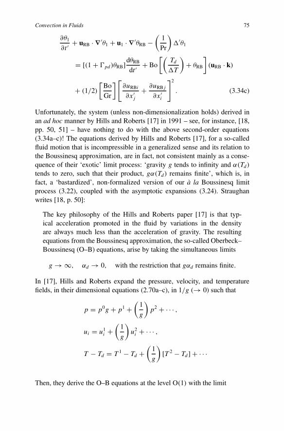
Convection in Fluids 75
∂θ1
∂t ′+ uRB · ∇′θ1 + u1 · ∇′θRB −
(1
Pr
)�′θ1
= [(1 + �pd)θRB]dθRB
dt ′+ Bo
[(Td
�T
)+ θRB
](uRB · k)
+ (1/2)
[Bo
Gr
] [∂uRBi
∂x′j
+ ∂uRBj
∂x′i
]2
. (3.34c)
Unfortunately, the system (unless non-dimensionalization holds) derived inan ad hoc manner by Hills and Roberts [17] in 1991 – see, for instance, [18,pp. 50, 51] – have nothing to do with the above second-order equations(3.34a–c)! The equations derived by Hills and Roberts [17], for a so-calledfluid motion that is incompressible in a generalized sense and its relation tothe Boussinesq approximation, are in fact, not consistent mainly as a conse-quence of their ‘exotic’ limit process: ‘gravity g tends to infinity and α(Td)
tends to zero, such that their product, gα(Td) remains finite’, which is, infact, a ‘bastardized’, non-formalized version of our à la Boussinesq limitprocess (3.22), coupled with the asymptotic expansions (3.24). Straughanwrites [18, p. 50]:
The key philosophy of the Hills and Roberts paper [17] is that typ-ical acceleration promoted in the fluid by variations in the densityare always much less than the acceleration of gravity. The resultingequations from the Boussinesq approximation, the so-called Oberbeck–Boussinesq (O–B) equations, arise by taking the simultaneous limits
g → ∞, αd → 0, with the restriction that gαd remains finite.
In [17], Hills and Roberts expand the pressure, velocity, and temperaturefields, in their dimensional equations (2.70a–c), in 1/g (→ 0) such that
p = p0g + p1 +(
1
g
)p2 + · · · ,
ui = u1i +
(1
g
)u2
i + · · · ,
T − Td = T 1 − Td +(
1
g
)[T 2 − Td ] + · · ·
Then, they derive the O–B equations at the level O(1) with the limit

76 The Simple Rayleigh (1916) Thermal Convection Problem
εH−R = gαdd
Cpd
→ 0.
In fact, their small parameter, εH−R, is our above εBo!Their derived equations are
∂ui
∂xi= 0,
du1i
dt= −RaT 1δi3 − ∂p1
∂xi+�u1
i ,
dT 1
dt− εH−R(Td + T 1)u1
3 =(
1
Pr
)�T 1 +
(2
Ra
)εH−Rd
1ij d
1ij .
However, these Hills and Roberts equations above contain (some) first-ordereffects of compressibility via the εH−R terms – the various terms in theseequations being very poorly balanced and, unfortunately, consistent (andgive only our RB model equations) only when their εH−R → 0.
We see that, even if an ad hoc derivation is often able to give a valuableresult at the leading order, in spite of the fact that a deficient approach hasbeen chosen, such an approach will in no way be able to derive consistentlya rational second-order approximation with well balanced second-order εterms. This strong observation is one of the main reasons for our presentapproach and for the publication of this book!
3.7 Some Comments
We have already observed that, for a rational formulation of the RB thermalconvection model equations, the smallness of the Froude number is a req-uisite condition which makes it possible to take into account the buoyancyas a main (Archimedean) driving force in this shallow thermal convectionmodel problem. But, this constraint has also an important consequence onthe upper, free-surface, condition relative to pressure p!
Namely, this upper boundary condition, (2.42a) written in Section 5.5,where dij are given by (2.2) in Chapter 2, is
p = pA + µ0[dij ninj − (2/3)(∇ · u)] + σ (T )(∇‖ · n),
at z = d + ah(t, x, y).

Convection in Fluids 77
With the non-dimensional quantities (3.6a–d) this above upper boundarycondition for the pressure is rewritten relative to the dimensionless pressure,
π =(
1
Fr2d
)[(p − pA)
gdρd
]+ z′ − 1,
in the dimensionless form
π1+ηh′ =(η
Fr2d
)h′(t ′, x′, y′)+ · · · . (3.35)
We do not have write the above dimensionless, upper, free-surface condition(3.35) for π at z′ = 1 + ηh′ in detail (this is done in Chapter 4). For themoment, the important point here is just the first term in condition (3.35) forπ1+ηh.
Indeed, because Fr2d � 1 for a rational derivation of the RB model equa-
tions, it is obvious that a necessary condition (in the framework of an asymp-totic modeling of the shallow thermal convection) for a rational approach isthe following:
η � 1, (3.36a)
with the similarity ruleη
Fr2d
≡ η∗ ≈ 1, (3.36b)
when the free-surface amplitude η and square of the Froude number, Fr2d ,
both tend to zero. In this case, for the shallow thermal convection modellimit, equations (3.25a–c), the upper boundary conditions are written (again)for a non-deformable free-surface, simulated by z′ = 1.
As a consequence, in a shallow thermal convection problem, when buoy-ancy is the main (Archimedean) driving force, in the leading order, the freesurface deformation has no influence.
On the other hand, for the dimensionless temperature θ , such that T =Td + (Tw − Td)θ , at the undeformable free-surface z′ = 1, we can write asan upper boundary condition (rigid-free problem) for the convection modelequations (3.25a–c),
∂θRB
∂z′
∣∣∣∣z′=1
= −1, (3.37)
when the Biot effect is neglected. But, from two upper, free-surface, condi-tions (2.42b, c),

78 The Simple Rayleigh (1916) Thermal Convection Problem
µddij (t(1))inj =[
dσ (T )
dT
](t(1))i
(∂T
∂xi
);
µddij (t(2))inj =[
dσ (T )
dT
](t(2))i
(∂T
∂xi
),
at z = d + ah(t, x, y),
rewritten with the non-dimensional quantities (3.6a–d) when the Marangonieffect is neglected and (3.36a, b) is taken into account, we obtain from(2.44a–c), instead of these above two tangential conditions, at z′ = 1:
∂u′1
∂z′ + ∂u′3
∂x′2
= 0,
∂u′2
∂z′ + ∂u′3
∂x′1
= 0,
and from the kinematic condition (2.38), again, with (3.36a, b), we have only
u′3 = 0, at z′ = 1. (3.38a)
As a consequence, at z′ = 1 we obtain two conditions:
∂u′1
∂z′ = 0, (3.38b)
and∂u′
2
∂z′ = 0. (3.38c)
Finally, from the second, divergence free condition, ∇′ · uRB = 0, for thevelocity vector in the shallow convection model equation (3.25b), and con-dition (3.38a–c), we obtain the following two upper, free-surface conditionsat z′ = 1:
wRB = 0, (3.39a)
and∂2wRB
∂z′2 = 0 (3.39b)
for the shallow convection model equations (3.25a–c).The three conditions (3.37) for θRB and (3.39a, b) for wRB at z′ = 1, re-
place the condition uRB = 0 and θRB = 1 at z′ = 1, written in (3.25d), whenwe consider for the RB equations (3.25a–c) a rigid-free model problem. Thisrigid-free, RB, model problem is the only significant limiting approximate

Convection in Fluids 79
problem, emerging rationally from the full Bénard exact problem (heatedfrom below) when we take into account a deformable free surface.
In Chapter 4, devoted to the full Bénard thermal convection problem,heated from below, we give a complete account of the Weber, Biot andMarangoni effects. We only observe here that an explicit and detailed ac-count of boundary conditions – especially at the upper, deformable free-surface – is indeed a matter of prime importance. A rigid conducting surfacebehaves in a drastically different way from a free and insulating surface. Themore significant (but difficult) case being, obviously, the thermal interactionof the fluid layer with the eventual boundary.
Concerning the Biot effect, the formal limit Biot ↓ 0, roughly, corre-sponds to the extreme situation of a perfectly conducting boundary. In thecase of an upper surface open to the air – a free-surface – from the thermalpoint of view the exchange of energy is affected by means of radiation, con-duction, and convection. These three phenomena together can be accountedfor by a so-called Robin condition that merely reduces to condition (2.46)or (2.47), or else (2.51). We observe that often the condition at a free sur-face for the temperature is written under the hypothesis, Td = TA, at the freesurface – between the passive air and the liquid the continuity of the temper-ature distribution is assumed but this seems rather a non-realistic hypothesis!As in [9] the more realistic upper, free surface condition is linked with thecontinuity of the heat flux across the free surface.
Quantitative, as well as qualitative, differences in behavior are to be ex-pected between the two extreme cases (Biot ↓ 0 and Biot ↑ ∞) of highlyconducting and insulating boundaries – in the former a fluctuation of tem-perature carried to the boundary soon relaxes through the exterior ambientair and, for a discussion from the physicist’s point of view, see the surveypaper by Normand et al. [19, pp. 597–598].
On the other hand, the quantity βs (> 0), which is defined as the nega-tive of the vertical conduction temperature gradient, −dTs(z)/dz, that wouldappear in a purely conductive state (since in the pure heat conducting state,the temperature at the upper surface is uniform), there is no ambiguity indetermining experimentally
�T = dβs = Tw − Td
and, according to (1.21b) with (1.21c), we have the following formula:
βs = (Tw − TA)
[(kd/qs)+ d] . (3.40)

80 The Simple Rayleigh (1916) Thermal Convection Problem
For more details, the reader is referred to Koschmieder and Prahl’s 1990work [20]. We stress again that when the fluid (the expansible liquid) is setin motion, the conduction temperature gradient βs is no longer the temper-ature gradient in the liquid layer since convection induces a non-zero meanperturbative temperature at the upper fluid surface.
As a consequence (as is pertinently observed in a paper by Parmentier etal. [21]) of this ‘obvious fact’, the dimensionless Marangoni and Rayleighnumbers (see definitions (1.19d) and (3.2)) must be experimentally evalu-ated with βs as given by (3.40), where qs is present. It is easily seen that the‘problem with two Biot numbers’ (outlined in Chapter 2) should be ques-tioned seriously (see also the discussion in Chapter 4), but a quantitativeand accurate description of this problem requires specific and likely lengthytreatments, which are outside the scope of the present book.
In general, the density ρ as a (solely) function of T , according to equationof state ρ = ρ(T ), can be written approximately as (see (2.39)):
ρ = ρ(T ) = ρd
{1 − α(Td)(T − Td)
+ (1/2)
[α2(Td)−
(∂α(T )
∂T
)Td
](T − Td)
2 + · · ·}, (3.41)
when an expansion in a Taylor’s series, about a constant temperature refer-ence (fiducial), Td , is performed. With (3.41), the main problem concernsthe influence of the term proportional to (T − Td)
2, when we want to derivea second-order approximate model. In a first naive approach we can write(3.41) in the following dimensionless form:
ρ
ρd≡ ρ ′(θ) = 1−εθ+(1/2)
[1 −
(1
α2d
)(∂α(T )
∂T
)Td
]ε2θ2+· · · . (3.42)
With (3.42), in the second-order set of equations (3.32a–c), various newterms appear. For example, first in equations (3.32a) for u1 on the right-handside, we have the following complementary term:
−(1/2)
[1 −
(1
α2d
)(∂α(T )
∂T
)Td
]Gr θ2
RBk, (3.43a)
but it is not clear: what is the value of the coefficient:(1
α2d
) (∂α(T )
∂T
)Td
. (3.43b)

Convection in Fluids 81
in (3.42), for various liquids?However, it seems (see the paper by Perez and Velarde [22]) that this coef-
ficient may have an effect on the second-order complementary term (3.43a),in the equation for u1! On the other hand, in [23] Knightly and Sather con-sider in an ad hoc manner a quadratic term in θ , in the leading-order shallowthermal convection equations. For this, according to (3.42), it is obviouslynecessary that
ε2
(1
α2d
) (∂α(T )
∂T
)Td
= εϕd (3.44a)
with
ϕd ≡(�T
αd
) (∂α(T )
∂T
)Td
(3.44b)
and in such a case, instead of the RB leading-order equation (3.25a) for uRB,we obtain the following shallow thermal convection model equation for uSh:
duSh
dt ′+ ∇′πSh − Gr
[θSh +
(ϕd2
)θ2
Sh
]k = �′uSh, (3.45)
which is a leading-order thermal shallow convection equation for the velocityuSh, analogous of one considered in [23] – but, obviously, more investigationinto this way is necessary.
Concerning the various analyses for RB convection, the reader can findrecent developments in a review paper by Boenschatz et al. [24]. In a shortpaper by Manneville [25] on the same subject and written 100 years later (inFrench) for the Journée H. Bénard, ESPCI, 25/06/2001, the reader can findalso a digest concerning various facets of RB convection, such as linear andnonlinear convection from Rayleigh to Busse, a physicist approach, transi-tion to chaos, the Newell–Whitehead–Segel-amplitude equations approach,with various references (in particular, [26–30]). Chapter 10 in [6], is devotedentirely to ‘asymptotic modelling of thermal convection (RB model) and in-terfacial phenomena (Marangoni effect and BM model)’.
In Chapters 5 to 7 we return carefully to three main convection modelproblems: RB, BM and deep-à la Zeytounian, and these three model convec-tion problems are also the main subject of the discussion in Chapter 8.
I shall close this chapter, by quoting a few lines extracted from a recentpaper by Paul Germain [31], which concerns very directly our above ap-proach related to the rational obtention of the second-order thermal convec-tion model equations. According to Germain [31]:
. . . it seems of great importance that a rational approach be adopted tomake sure, for example, that terms neglected really are much smaller

82 The Simple Rayleigh (1916) Thermal Convection Problem
than those retained. Until this is done, and even now it is possible inpart, it will be difficult to convince the detached and possibly skepticalreader of their value as an aid to understanding.
On the other hand, from [6, p. xv] we quote:
For some time the growth in capabilities of numerical simulation influid dynamics will be strongly dependent on, or at least closely relatedto, the development of the rational modelling.
References
1. Lord Rayleigh, On convection currents in horizontal layer of fluid when the higher tem-perature is on the under side. Philos. Mag. Ser. 6 32(192), 529–546, 1916.
2. H. Bénard, Les tourbillons cellulaires dans une nappe liquide. Revue Gén. Sci. PuresAppl. 11, 1261–1271 and 1309–1328, 1900. See also: Les tourbillons cellulaires dansune nappe liquide transportant de la chaleur par convection en régime permanent. Ann.Chimie Phys. 23, 62–144, 1901.
3. J. Boussinesq, Théorie analytique de la chaleur, Vol. II. Gauthier-Villars, Paris, 1903.4. R.Kh. Zeytounian, Joseph Boussinesq and his approximation: A contemporary view.
C.R. Mec. 331, 575–586, 2003.5. S. Chandrasekhar, Hydrodynamic and Hydromagnetic Stability. Clarendon Press, Ox-
ford, 1961. See also Dover Publications, New York, 1981.6. R.Kh. Zeytounian, Asymptotic Modelling of Fluid Flow Phenomena. Fluid Mechanics
and Its Applications, Vol. 64, Kluwer, Dordrecht, 2002.7. E.L. Koschmieder, Bénard Cells and Taylor Vortices. Cambridge University Press, Cam-
bridge, 1993.8. M.J. Block, Nature 178, 650–651, 1956.9. J.R.A. Pearson, On convection cells induced by surface tension. J. Fluid Mech. 4, 489,
1958.10. E. Guyon, J-P. Hulin, L. Petit and C.D. Mitescu, Physical Hydrodynamics. Oxford Uni-
versity Press, Oxford, 2001.11. R.Kh. Zeytounian, The Bénard–Marangoni thermocapillary instability problem: On the
role of the buoyancy. Int. J. Engrg. Sci. 35(5), 455–466, 1997.12. R.Kh. Zeytounian, The Bénard–Marangoni thermocapillary-instability problem, Phys.
Uspekhi 41(3), 241–267, 1998 [English edition].13. P.G. Drazin and W.H. Reid, Hydrodynamic Instability. Cambridge University Press,
Cambridge, 1981.14. R.Kh. Zeytounian, Theory and Applications of Viscous Fluid Flows. Springer-Verlag,
Berlin/Heidelberg, 2004.15. A. Pellew and R.V. Southwell, Proc. Roy. Soc. A176, 312–343, 1940.16. D.D. Joseph, Stability of Fluid Motions, Vol. II. Springer, Heidelberg, 1976.17. R. Hills and P. Roberts, Stab. Appl. Anal. Continuous Media 1, 205–212, 1991.18. B. Straughan, The Energy Method, Stability, and Nonlinear Convection. Appl. Math. Sci.
Vol. 91. Springer-Verlag, New York, 1992.

Convection in Fluids 83
19. C. Normand, Y. Pomeau and M.G. Velarde, Convective instability: A physicist’s ap-proach. Rev. Modern Phys. 48(3), 581–624, 1977.
20. E.L. Koschmieder and S. Prahl, J. Fluid Mech. 215, 571, 1990.21. P.M. Parmentier, V.C. Regnier and G. Lebond, Nonlinear analysis of coupled gravita-
tional and capillary thermoconvection in thin fluid layers. Phys. Rev. E 54(1), 411–423,1996.
22. R. Perez Cordon and M.G. Velarde, J. Physique 36(7/8), 591–601, 1975.23. G.H. Knightly and D. Sather, Stability of Cellular Convection, Archive for Rational Me-
chanics and Analysis 97(4), 271–297, 1987.24. E. Boenschatz, W. Pesch and G. Ahlers, Ann. Rev. Fluid Mech. 32, 708–778, 2000.25. P. Manneville, Convection de Rayleigh–Bénard. Journée H. Bénard, ESPCI, Paris 25/06,
2001.26. F.H. Busse, Transition to turbulence in thermal convection. In: Convective Transport and
Instability Phenomena, J. Zierep, H. Oertel (Eds.). Braun, Karlsruhe, 1982.27. A.C. Newell, Th. Passot and J. Legat, Ann. Rev. Fluid Mech. 25, 399–453, 1993.28. P. Bergé, Nucl. Phys. B (Proc. Suppl.) 2, 247–258, 1987.29. Y. Pomeau and P. Manneville, J. Phys. Lettr. 40, L-610, 1979.30. P. Manneville, J. Physique, 44, 759-765, 1983.31. P. Germain, The ‘new’ mechanics of fluids of Ludwig Prandtl. In: Ludwig Prandtl, ein
Führer in der Strömungslehre, G.E.A. Meier (Ed.), pp. 31–40. Vieweg, Braunschweig,2000.

Chapter 4The Bénard (1900, 1901) Convection Problem,Heated from Below
4.1 Introduction
In this chapter, we take into account the influence of a deformable free sur-face and, as a consequence, we revisit the mathematical formulation of theclassical problem describing the Bénard instability of a horizontal layer offluid, heated from below, and bounded by an upper deformable free sur-face. Because the deformation of the free surface, subject to a temperature-dependent surface tension, is taken into account in the full Bénard convectionproblem, heated from below, we have not specified this convection as beinga ‘thermal convection’.
Indeed, in the full starting Bénard problem, heated from below, when wetake into account the influence of a deformable free surface, subject to atemperature-dependent surface tension, the fluid being an expansible liq-uid, it is necessary to take into account, simultaneously, four main effects.Namely:
(a) the conduction adverse temperature gradient (Bénard) effect in motion-less steady-state conduction temperature,
(b) the temperature-dependent surface tension (Marangoni) effect,(c) the heat flux across the upper, free surface (Biot) effect, and(d) the buoyancy (Archimedean–Boussinesq) effect arising from the vol-
ume (gravity) forces.
Particular attention is also paid to the approximate form of the equation ofstate for a weakly expansible liquid.
In his two pioneering papers [1], Henri Bénard (1900, 1901) considereda very thin layer of fluid, about a millimeter in depth, or less, standing ona levelled metallic plate maintained at a constant temperature. The upper
85

86 The Bénard Convection Problem, Heated from Below
surface was usually free and, being in contact with the air, was at a lowertemperature. Bénard experimented with several liquids of differing physicalconstants. He was particularly interested in the role of viscosity (in fact, liq-uid with a high viscosity and a low Reynolds number, which is linked withthe lubrication approximation).
In all cases, Bénard found that when the temperature of the lower platewas gradually increased, at a certain instant the layer became reticulated andrevealed its dissection into cells. Concerning the experiments on the onset of(thermal) instability in fluids, see [2, pp. 59–75], and also the more recentbook by Koschmieder [3].
More precisely, the Bénard cells are primarily induced (in a very thin layerof expansible liquid) by the temperature-dependent surface tension gradi-ents resulting from temperature variations on the deformable free surface.The corresponding instability phenomenon is usually known as the Bénard–Marangoni (BM) thermocapillary instability. The first scientist whose worksenlightened the way to our understanding of surface tension gradient-drivenflows was Carlo Marangoni (1865, 1871), in [4], who was known to havelively exchanges with Joseph Plateau (1849, 1873), see [5].
Unfortunately, the Bénard cells phenomenon was confused (over thecourse of many years) with the well-known Rayleigh–Bénard (RB) buoy-ancy driven instability according to Rayleigh’s (1916) interpretation, via theso-called Boussinesq approximation (1903), and assuming (as in Chapter 3)that the fluid is confined between two planes, the influence of the deforma-tion of a free surface being completely eliminated! Indeed, the RB instabilityappeared in situations when the liquid layer, with a substantial thickness, isbounded by a flat (non-deformable) upper, free surface, the buoyant volume(Archimedean) forces being the main driving operative effect. See in [6],Zeytounian’s alternative which is quoted in Section 3.1.
The inappropriateness of Lord Rayleigh’s (1916) model to Bénard’s ex-periment was not adequately explained until Pearson in 1958 [12] showed (inan ad hoc linear theory) that, rather than being a buoyancy driven flow, Bé-nard cells are the consequence of a temperature-dependent surface tension.However, we observe that, two years before Pearson, in 1956, Block [8] ina short (2 pages) paper showed that: ‘tension [is] the cause of Bénard cellsand surface deformation in a liquid film’ and ‘when a liquid film (about 0.08cm thick) with a free surface was cooled at its base, cellular patterns moreregular than Bénard cells were observed’.
Of course in practice, usually, both the buoyancy effect (in the liquid layer)and the temperature-dependent surface tension effect (on a free deformablesurface) are operative, so it is natural to ask: how are the two effects coupled?

Convection in Fluids 87
Along this line, Nield [7] combined both mechanisms into a single (rathersimple) analysis and found that: ‘as the depth of the liquid layer decreases,the surface tension mechanism becomes more dominant and when the depthof the layer is less than 0.1 cm the buoyancy effect can safely be neglectedfor most liquids’.
In reality, all the above assertions are true only in the leading order for aweakly expansible liquid, in the framework of an approximate rational theoryand asymptotic modelling.
This role of surface tension cannot be explained by existing theories inwhich the free surface is assumed to be flat – non-deformable – and only in1997, via a coherent, asymptotic modelling [9] was I able to prove consis-tently my ‘alternative’ [6], which is based on the value of the squared Froudenumber
Fr2d = (νd/d)
2
gd, (4.1)
where d is the thickness of the fluid layer in the motionless state, νd theconstant kinematic viscosity (dependent on the constant temperature Td ) andg the magnitude of the gravity force.
More precisely, when Fr2d = O(1), and in such a case d ≈ 1 mm, at the
leading order we derive the BM problem and, for Fr2d � 1, at the leading
order, we derive the RB problem, with an upper bound for the thickness(d), when we do not take into account (at the leading order) the term withthe viscous dissipation function in the full energy equation written for thedimensionless temperature θ of the liquid.
On the other hand, in our asymptotic rational analysis, the main small(expansibility) parameter (where �T = dβs , with βs the adverse conductiontemperature gradient),
ε = αd�T, (4.2)
is linked with the weakly thermal expansion (αd is the cubic dilatation attemperature Td) of the liquid and the classical Grashof number,
Gr = ε
Fr2d
, (4.3)
a ratio of ε to Fr2d , is in fact a similarity parameter (the ratio of two small
parameters). We note that in some works devoted to thermal convection thenon-dimensional expansibility, small parameter ε is called a ‘Boussinesq’number and
Ga = Pr
Fr2d
≡ (νd/κd)gd
(νd/d)2= gd3
νdκd(4.4)

88 The Bénard Convection Problem, Heated from Below
is a ‘Galileo’ number, where Pr is the Prandtl number – the ratio of kinematicviscosity νd and thermal diffusivity κd . In such a case the Rayleigh number
Ra = αd�Tgd3
νdκd≡ εGa (4.5)
appears as the product of a Boussinesq number αd�T , with a Galileo numberGa, defined by (4.4).
As a consequence, if a situation is considered for which the aboveRayleigh number (4.5) is of order unity or higher, the use of the Boussinesqapproximation (and in such a case the driving force in thermal convection isthe buoyancy term) implies Ga � 1, because ε � 1.
Typical values of the Prandtl number Pr are the following:
• for water = 6; silicone oil = 5 × 10⁴; mercury = 0.026; air = 0.7;• for liquids used for experiments on Bénard instabilities = 5 or more,
especially for highly viscous oils;• for liquid metals = 10−2–10−3;• for gases ≈ 1.
For a consistent derivation of the shallow convection (Boussinesq) equationsgoverning the RB problem (where, in fact, ρ = ρ(T )) it is necessary to takeinto account a second similarity relation (see (2.30)) between the small, ex-pansibility parameter ε and the small isothermal compressibility coefficient� (defined by (2.29)) such that
ε2
� ≡ K0 = O(1). (4.6)
Some aspects of the interfacial phenomena – Marangoni and Biot effects –have been discussed in [6] and, more recently, in [10].
From the above brief discussion, we see that the RB and BM instabilitymodel problems are both limiting cases of the full classical Bénard, heatedfrom below, instability problem, when we assume that the liquid is weaklyexpansible, the Froude number being small or O(1). This point of view al-lows us to formulate both these convection problems in a coherent way and,if necessary, to derive the corresponding second-order model approximateproblems which take into account the influence of a weak expansibility andviscous dissipation of the liquid – a third type of convection, named ‘deepconvection’ (DC) in [17], emerges also (see Chapter 6) from this full classi-cal Bénard instability problem, heated from below. We observe, for instance,that our consistent asymptotic approach gives (unexpectedly) the possibilityto obtain, in the framework of the RB problem, a partial differential equation

Convection in Fluids 89
for deformation of the free surface (which depends on a Weber number as-sumed to be large and linked with the constant part of the surface tension, see(1.28a, b)) via the dimensionless pressure at an upper non-deformable freesurface which is a known function, when the RB model problem is resolved.
In practice, the first fundamental effect in the full Bénard thermal insta-bility problem is strongly related to the definition of the adverse conductiontemperature gradient βs in motionless steady-state conduction temperatureTs(z), where z is the vertical (to z = 0, lower heated horizontal solid plane)coordinate in the direction of the unit vector k (see Section 4.2). For thedefinition of βs , via the data of the Bénard problem, it seems necessary (asrealized in Chapter 1, see (1.20)–(1.21)) to introduce a constant conductionheat transfer coefficient qs and write the corresponding Newton’s cooling law(see equation (4.12b)) for the motionless conduction-steady (function onlyof z) temperature, Ts(z) = Tw − βsz, at z = d, which places the mean, flat,position of the free surface in a steady-state motionless conduction regime.In Section 4.4, we consider another scenario related to the dimensionlesstemperature (1.17c)/(2.48),
� = (T − TA)
(Tw − TA),
the temperature-dependent surface tension being modeled by the linear ap-proximation (2.52) with (2.53)
σ (T ) = σ (T A)− γσ (T − TA), with γσ = −[
dσ (T )
dT
]at T = TA,
in a convective regime; this model for temperature-dependent surface tensionhas been used in various recent papers.
The lower heated plate temperature Tw = Ts(0) being a given data, in thiscase, the adverse conduction temperature gradient βs appears as a knownfunction of (Tw−TA), where TA (< Tw) is the known temperature of the pas-sive air far above the free surface when the conduction constant Biot number
Bis = dqs(Td)
kd, (4.7)
with a constant thermal conductivity kd , and the constant qs(Td), is known(see in Chapter 1, (1.21b) and (1.22)). Here, we use the reference temperature
Ts(z = d) ≡ Td = Tw − βsd, (4.8)
and it is clear that βs is always different from zero in the framework of theBénard instability problem heated from below, and as a consequence in what

90 The Bénard Convection Problem, Heated from Below
follows it is necessary to have in mind that, always, the conduction Biotnumber, defined by (4.7), is also different from zero: Bis �= 0!
This trivial remark has, in fact, an important consequence and shows(again) that it is necessary, without fail, to work with the two Biot numbers– the first being the above constant conduction Biot number Bis , definedby (4.7). The second (in general variable) convective Biot number, beingstrongly linked with the formulation of the thermocapillary BM convectivemodel problem, where again Newton’s cooling law is used to obtain a bound-ary condition on a free deformable surface z = H(t, x, y) for the dimension-less temperature (see Section 2.5)
θ = (T − Td)
�T, with Tw − Td ≡ �T , (4.9)
(or �), but with a (variable, second) heat transfer convection coefficient,qconv; see for instance (1.23b).
We again observe that in the framework of an approach à la Davis [11],but with two Biot numbers, the correct upper boundary condition for thedimensionless temperature θ (defined by the relation (4.9)) is the dimension-less condition (2.46), where Biconv is a non-constant convective Biot number!Only (2.46) is the correct condition for θ , contrary to the Davis condition(2.47) where Bis and Biconv = dqconv/kd are replaced by a single B (surfaceBiot number, with a unit thermal surface conductance h instead of our qconv).
Obviously, as a first tentative approach, we can assume that Biconv is afunction of temperature T of the liquid or else a function of the full thick-ness H(t, x, y) of the deformable thin film. In such a case, it seems judiciousto assume that the associated constant conduction Biot number Bis is (whenthe deformation of the free surface is absent) respectively, a function of Td ,Bis(Td ), or else a function of d, Bis(d). As has been noted in Section 2.5,the assumption concerning the necessity to introduce a variable convectiveheat transfer coefficient is present in the pioneering paper by Pearson [12],where a small disturbance analysis is carried out. On the other hand, for athin layer with strong surface deformation (nonlinear case) and, especially,in the framework of the derivation of the lubrication equation, via the long-wave approximation (see Sections 7.3 and 7.4), a dependence of qconv on thefull thickness H(t, x, y) seems reasonable (see, for instance, the pertinentpaper by Vanhook et al. [13]). It is also important to observe that we have as-sumed above that the conduction heat transfer coefficient qs = const and, asa consequence, Bis = const, because the reference temperature Td = constis uniform along the flat free surface, z = d, in the conduction regime linkedwith the motionless steady-state temperature Ts(z) = Tw − βsz. Obviously,

Convection in Fluids 91
as has been stressed in Section 3.7, this is no longer true in thermocapillaryconvective instability because the dimensionless temperature θ , at the upperdeformable free surface z = H(t, x, y), varies from point to point. The heattransfer convective coefficient qconv or its dimensionless expression, the con-vection Biot, Biconv, number, is then not a constant (see, again, the discussionin [14,15]). Therefore, it seems necessary to work with these two Biot num-bers, Bis and Biconv, according to the upper, free-surface condition (2.46) forθ .
This leads to some modifications in the formulation of the BM modelproblem and its various applications – but, when we identify Biconv with Bis(as is the case in [11]) we recover again Davis’ condition, derived in 1987,and from our results it is possible to obtain again some usual results.
These common results, obtained with a single (conduction) Biot numberin the linear theory, are questionable (at least from a logical point of view)for the case of a zero Biot (convection) number. The conduction (differentfrom zero) Biot number allows us (in the case of a Bénard convectionin a thin liquid layer with an upper deformable free surface) to define βsaccording to (1.21b).
I do not claim that our approach is the more effective approach or that itresolves the ‘two Biot numbers paradox’, which deserves obviously furthercareful attention. But I observe that our derived boundary condition (2.46)with two Biot numbers, seems to me more appropriate and justified. In anycase, our condition (2.46) is the only correct one when we use Davis’s [11]‘imaginative, 1987, approach’ – but without Davis’s confusion, which iden-tifies Biconv with Bis . From another point of view, it is also possible to replaceDavis’s (derived in [11]) upper condition (2.47) for θ , by the à la Pearsoncondition (2.51) for dimensionless temperature �. In this upper, free surface,at z′ = 1 + ηh′(t ′, x′, y′), dimensionless condition, the parameter L is, infact, a convective Biot number,
L =(
d
kd
)[dQ(T )
dT
]A
. (4.10)
Finally, as the upper, free-surface condition for �, it is also adequate to usedirectly the condition (2.37)!
We now devote Section 4.2 to a detailed dimensionless mathematical for-mulation of the full Bénard, starting, exact convection problem heated frombelow. In this mathematical dimensionless, starting formulation, the buoy-ancy (Rayleigh–Bénard) and thermocapillary (Marangoni) are the two main

92 The Bénard Convection Problem, Heated from Below
effects taken into account. In this starting dimensionless problem the We-ber and Biot numbers are also present, as well as the Boussinesq numberlinked with the viscous dissipation term; the upper, free surface, separatingthe passive air from the liquid layer, is assumed deformable.
In Section 4.3 we will show the fundamental role played by the Froudenumber, in the case of a weakly expansible liquid, for a consistent derivationof two main approximate rational models: first, in the buoyancy driven shal-low thermal convection model RB equations and associated upper boundaryconditions, then in the thermocapillary convection BM model problem witha deformable free surface.
The role of the Boussinesq number, Bo (defined by (1.16)), in the case ofthe deep thermal convection model problem with viscous dissipation term,is also considered in Section 4.3. However, the case of ultra-thin films is notconsidered in this book (see the references at the end of Chapter 10).
Finally, in Section 4.4 the reader can find some complements and con-cluding remarks. First, we consider the upper, free-surface, boundary con-dition (at z′ = 1 + ηh′(t ′x′
1, x′2)) for the dimensionless temperature, � =
(T−TA)/(Tw−TA), instead of θ . Then, a discussion relative to long-wave ap-proximation used in lubrication theory is given. Finally, we consider brieflysome film flows in various geometries, for example, down an inclined planeand a vertical plate, down inside a vertical circular tube, coating of a liquidfilm, over a substrate with topography, liquid hanging below a solid ceiling,etc.
4.2 Bénard Problem Formulation, Heated from Below
We consider the horizontal one-layer classical Bénard problem, heated frombelow, consisting of a (weakly) expansible viscous and heat conductor liq-uid bounded below by a rigid horizontal flat surface (a plate) and above bya passive gas (an ambient air having negligible density, viscosity and knownconstant pressure (pA) and temperature (TA) far from the free surface) sep-arated by a deformable free surface. This free surface, separating the liquidlayer from the passive ambient air, in conduction motionless steady conduc-tion state coincides with the flat plate z = d, the thickness of the liquid layerin conduction state being d. The rigid plate z = 0 is a perfect heat conductorfixed at temperature Tw and the free surface (non-dimensional equation), inthe convection process is
z
d≡ z′ = 1 + ηh′(t ′, x′
1, x′2), (4.11)

Convection in Fluids 93
Fig. 4.1 Geometry of the full Bénard thermal convection problem.
with η ≡ a/d, the amplitude parameter of the deformable (with as a dimen-sionless free surface deformation function, h′(t ′, x′
1, x′2). The geometry of
the full Bénard thermal convection problem is sketched in Figure 4.1.The various non-dimensional quantities (denoted by a prime were intro-
duced in Section 3.3 by (3.6a–d)). In the case of a strong deformation of thefree surface, in the nonlinear case, we assume that η = O(1). In a steady-state motionless conduction state, when the temperature is Ts(z), we obtain(with k ≡ kd = const) the following simple conduction problem (see, forinstance, Section 4.3):
d2Ts(z)
dz2= 0, with Ts(0) = Tw, (4.12a)
and
kddTs(z)
dz+ qs[Ts(z)− TA] = 0, at z = d. (4.12b)
The condition at z = d being the usual Newton’s cooling law, but writ-ten for the steady-state temperature Ts(z) in a conduction motionless regime,when the free surface is flat, z = d. Thanks to Newton’s cooling law (4.12b)we are able to determine the adverse temperature gradient βs , in motion-less conduction steady state, via the constant (at constant temperature Td )heat transfer, conduction coefficient qs . Namely, the solution of (4.12a) with(4.12b) is obviously of the form (mentioned in the Introduction, Chapter 1,see (1.19a) and (1.21b)),
Ts(z) = Tw − βsz, with βs =[
Bis(1 + Bis)
][(Tw − TA)
d
], (4.12c)

94 The Bénard Convection Problem, Heated from Below
where the conduction Biot number Bis is defined by (4.7). We observe alsothat if, in the starting Bénard problem, the given data are respectively d, qs ,kd (or Bis), Tw and TA, then when βs is defined by the above relation (validin the conduction regime) we determine also the reference temperature:
Ts(z = d) = Td = Tw − βsd,
and we have also
βs = (Tw − Td)
d≡ �T
d, or βs = Bis(Td)
[(Td − TA)
d
],
or else (4.12c) for βs .Since Bis is different from zero, in a similar manner βs is always also
different from zero. The reference temperature Td is obviously assumed dif-ferent from the air temperature TA and in such a case at the flat surface z = d
a discrete jump in temperature is realized! Indeed, the conduction Biot num-ber, Bis �= 0, defined above plays an important role in the mathematicalformulation of the Bénard dimensionless problem heated from below, andappears as a Bénard conduction effect which is always operating in convec-tion model problems – this point is rarely noted, as if the authors of variouspapers on film problems do not wish to raise doubts concerning this Biotproblem?
Finally, in the conduction steady motionless state, instead of (4.9), weobtain for the dimensionless conduction temperature:
θs(z′) ≡ [Ts(z′)− Td ]
(Tw − Td)= 1 − z′. (4.13)
Usually it is assumed that for the temperature-dependent surface tension σ =σ (T ), we have the following approximate equation of state (according to(1.17a, b)):
σ (T ) = σ (Td)− γσ (T − Td), where γσ = −dσ (T )
dT
∣∣∣∣T=Td
= const > 0,
(4.14)where Td is present, so that there is surface flow from the hot end toward thecold end and, since the bulk fluids are viscous, they are dragged along. As aconsequence bulk-fluid motion results from interfacial temperature gradient,a so-called Marangoni thermocapillary effect. With the references constantdensity ρd , viscosity νd , constant tension σ (Td) and constant tension gradientγσ , for our viscous liquid, we define the Marangoni and Weber numbers as

Convection in Fluids 95
Ma = γσβsd2
ρdν2d
, We = σ (Td)d
ρdν2d
. (4.15)
And instead of (4.14), we write
σ (T )
σ (Td)= 1 − (Ma/We)θ. (4.16)
Instead of the Weber number, according to the physicists usually a so-calledcrispation number (slightly ‘modified’, see also Section 3.3), the followingformula is introduced:
Cr = 1
We Pr= ρdνdκd
σ (Td)d(4.17a)
where Pr = νd/κd is the Prandtl number with κd the constant thermal diffu-sivity of the heat conductor liquid. For most liquids in contact with air, Cris very small and as a consequence the thermocapillary effect is significant(according to (4.16)) only for a relatively large modified Marangoni number
Ma = Pr Ma = γσβsd2
ρdνdκd
. (4.17b)
and see, for instance in [16, p. 2748], the parameter range of this crispation,Cr parameter. In fact, the modified Marangoni number, Ma, is the ratio of adriving force, due to change in the surface tension, to viscous frictional force.This driving force for the Marangoni effect acts only at the free surface ofthe fluid layer and, as a consequence, in the upper, free-surface, boundarycondition, at z = H(t, x, y), we have a complementary term (see (2.36c)):
∇‖σ (T ) =[
dσ (T )
dT
]∇‖T , (4.18)
where ∇‖ is a surface gradient defined only in the free surface by the relation(2.36a). Finally, it is important to note that the Marangoni effect, character-ized by the Marangoni number Ma, is operative only when Bis is differentfrom zero, or when the Bénard conduction effect is really taken into account(when at the flat surface, z = d, a discrete jump in temperature is realized);this follows from the relation (4.15) for Ma where βs is present.
Below, the system of three equations (2.32a–c), derived in Section 2.4, areour starting exact full equations, with dimensional quantities. Namely:
dρ
dt+ ρ(∇ · u) = 0, (4.19a)

96 The Bénard Convection Problem, Heated from Below
ρdu
dt+ ∇p = ρf + µd [�u + (1/3)∇(∇ · u)], (4.19b)
ρCp
dT
dt− αT
dp
dt= �+ kd�T, (4.19c)
with for density ρ, according to (2-32d), the following approximate equationof state is used:
ρ = ρd
{1 − ε
[(T − Td)
�T
]+
(1
K0
)ε2
[(p − pA)
gdρd
]}, (4.19d)
As upper boundary conditions (with dimensional quantities), at the free sur-face, we have the following set of four conditions, according to (2.38)–(2.42a–c); also see Section 2.5. Namely, at z = d + ah(t, x1, x2) ≡H(t, x1, x2) the kinematic condition is
d
dt[z −H(t, x, y)] = 0, (4.20a)
and the three jump conditions for the stress tensor are:
p = pA + µd
[(∂ui
∂xj+ ∂uj
∂xi
)ninj − (2/3)(∇ · u)
]+ σ (T )(∇‖ · n);
(4.20b)
µd
(∂ui
∂xj+ ∂uj
∂xi
)t(1)i nj =
[dσ (T )
dT
]t(1)i
(∂T
∂xi
); (4.20c)
µd
(∂ui
∂xj+ ∂uj
∂xi
)t(2)i nj =
[dσ (T )
dT
]t(2)i
(∂T
∂xi
). (4.20d)
For the non-dimensional temperature θ , given by (4.9), we write (see (2.46))our upper dimensionless boundary condition at z′ = 1 + ηh′(t ′, x′, y′) ≡H ′(t ′, x′, y′), as
∂θ
∂n′ +{
Biconv
Bis(Td)
}[1 + Bis(Td)θ] = 0, (4.20e)
where the convective, Biconv, Biot number is, in general, a non-constant pa-rameter and Q0 = 0.
In equation (4.19c) the viscous dissipation term � is given by
� = 2µd {D(u) : D(u)− (1/3)(∇ · u)2}, (4.21a)
and the term ρf ≡ −ρgk, the single body force being the gravity force. Onthe other hand, the kinematic condition (4.20a), written at z = H(t, x, y), isrewritten as

Convection in Fluids 97
u · k =[∂
∂t+ u1
∂
∂x1+ u2
∂
∂x2
]H(t, x1, x2). (4.21b)
In upper boundary condition (4.20b), for the pressure difference, p−pA, theterm, ∇‖ · n is given by (2.43a), with (2.43b–d). The outward normal unitvector n is given by (2.44c) and the two unit tangent vectors t(1) and t(2) inabove (4.20c, d), parallel to the upper, free surface z = H(t, x, y), are givenby (2.44a, b).
We observe also that, below as in Section 3.3, the dimensionless quantities(see (3.6a, b)) are denoted by a prime, and on the other hand the dimensionalCartesian coordinates are, in various parts of this book, designated by
x1 ≡ x, x2 ≡ y and x3 ≡ z.
In, upper, free-surface condition (4.20e) for θ , we have (see (3.6a, b) and(2.43b)), in dimensionless form:
∂θ
∂n′ = ∇′θ · n′ =(
1
N ′
)1/2 {∂θ
∂z′ − η(D′θ · D′h′)}, (4.22a)
where, in dimensionless form,
N ′ = 1 + η2D′2h′, n′ =(
1
N ′
)1/2 (−η∂h
′
∂x′ ; −η∂h′
∂y′ ; +1
), (4.22b)
∇′ =(∂
∂z′
)k + D′, with D′ =
(∂
∂x′ ;∂
∂y′
). (4.22c)
In a linear theory when
θ = 1 − z′ + ηθ ′(t ′, x′, y′, z′) + · · · , (4.23a)
and, when Biconv is assumed a function of H ′(t ′, x′, y′) ≡ 1 + ηh′(t ′, x′, y′),in a convective regime, we have the approximate relation
Biconv ≡ Bi(H ′(t ′, x′, y′)) = Bi(1)+ η�(H ′ ≡ 1)h′, (4.23b)
where
� = dBi
dH ′ , (4.23c)
and with Bi(1) ≡ Bis , we derive, instead of a full, upper, free-surface con-dition (4.20e) for θ , the following linear (at the order O(η) and written atz′ = 1), upper, free-surface condition for θ ′ in the convective regime

98 The Bénard Convection Problem, Heated from Below
∂θ ′
∂z′ + Bis(θ′ − h′)+
(1
Bis
)�(H ′ ≡ 1)h′ = 0, at z′ = 1. (4.23d)
In the above linearized, free-surface, boundary condition for θ ′, (4.23d), wehave again Bis , but not a Biot number related to the convection regime, infront of the term with (θ ′ − h′), as this is the case usually (see, for in-stance, [16, p. 2747]). On the other hand, we have a complementary termproportional to h′ which emerges from the variability of the convection Biotnumber! An accurate linearization shows easily that, in fact, it is not possibleto work with two constant Biot numbers, at least with the choice Q0 = 0.
Indeed, if Biconv ≡ Bi0const is a constant, then the linearization is possibleonly when we assume that
Q0 = kβS
[1 −
(Bi0conv
Bis
)], (4.23e)
and in such a case, and only for this case, we recover a linear, upper, free-surface condition for θ ′, à la Takashima [16],
∂θ ′
∂z′ + Bi0conv(θ′ − h′) = 0, at z′ = 1, (4.23f)
where, as a constant coefficient, in front of (θ ′ − h′) the constant convec-tive Biot number Bi0conv appears – obviously, in such a case, the results ofTakashima [16] are consistent when Bi0conv = 0, but not with Bis = 0!
Obviously, with the Davis’ approach [11], the classical linear theory, à laTakashima [18], with a (single conduction) Biot number equal to zero seemsquestionable. Our approach above, which gives (4.23f), explains clearly the‘zero (convective) Biot number case’ in linear theory.
It is necessary (in a simple case, for instance) to assume that the con-vection (in a convection regime, with a deformable free surface) Biot num-ber, Biconv, is a function of the full thickness of the liquid layer, H ′ ≡ 1 +ηh′(t ′, x′, y′), or a function of dimensionless temperature, θ(t ′, x′, y′, z′), orelse (at least) that Biconv is a function of the small parameter η, Biconv = B(η)
– especially in the linear theory. It is important to note, also we are not con-cerned here with a thorough analysis of the mechanism of heat transfer toand from the liquid layer, though these matters become relevant in the inves-tigations of any particular physical phenomenon. It must be made clear thatthe evaluation of Bi(H ′) in condition (4.23b) or �(H ′ ≡ 1) in linear con-dition (4.23d), in any physically observed circumstances is not necessarilyeasy – it is, however, a separate problem.
As observed by Pearson [12], the introduction of a different heat trans-fer coefficient, at least in the classical form of Newton’s cooling law, is of

Convection in Fluids 99
crucial importance and by means of a suitable choice many physical inter-facial phenomena may be very reasonably idealized. Obviously, the aim inthis account is not to provide an exhaustive description of these phenomenaand their relevant idealizations, but rather to provide a general treatment thatillustrates the fundamental surface tension mechanism and comprehends itsmany realizations.
In particular, the evaluation of the role of the second variable, Bi(H ′),convective Biot number on the lubrication equation (see, for instance, Sec-tion 4.4) is an interesting problem.
Finally, another advantage of the introduction of a second variable con-vective Biot number is the clear distinction between the Biot and Marangonieffects in the thermocapillary convection problem.
For me it is clear that it is necessary to strictly observe, first, at least in afundamental modelization of a physical phenomena (such as convection influids), the rigor and consistency of the elaborated theory and, above all,not to ‘adapt’ this theory for an eventual approximate evaluation of theconsidered physical phenomena – this is obviously often a difficult challengebut so fruitful in consequences!
It is necessary to add to the above equations (4.19a–c), with (4.19d) and(4.21a), and upper conditions (4.20a–e), the following condition for u and θat z′ = 0:
u = 0 and θ = 1. (4.24)
We observe also that, in the approximate equation of state (4.19d), for thedensity ρ, the constant K0 = O(1) is given by the following relation (whenwe use the relation (2.27), and definitions (1.10a), (2.29)):
K0 = Cvd(γ − 1)(�T )2
gdTd. (4.25a)
As a consequence, we obtain the following constraint for �T :
�T ≈[
gdTd
(γ − 1)Cvd
]1/2
, (4.25b)
when we assume thatK0 = O(1).
For the derivation of not only leading-order approximate equations, from theabove starting exact system for the full Bénard convection problem, heated

100 The Bénard Convection Problem, Heated from Below
from below, but also companion second-order approximate equations, a care-ful inspection shows that it is sufficient to use in exact equation (4.19c) forCp and α the relations (3.9a, b) with (3.10a, b).
Below, in the so-called ‘dominant’ dimensionless Bénard problem, wetake into account only the terms which are necessary for a rational and con-sistent derivation of these leading and second-order equations. The dimen-sionless quantities (with the prime) are given by (3.6a–d), but in relation(3.6c), for π , instead of p−pd we write obviously p−pA, because we takethe existence of a deformable upper, free surface into account.
First, with the approximate equation of state (4.19d), instead of the con-tinuity equation (4.19a) we can write the following dominant dimensionlessequation of continuity:
∇′ · u′ = εdθ
dt ′, (4.26a)
the term (ε2/K0)[Fr2ddπ/dt ′ −u′
3], on the right-hand side (see (4.19d)) beingneglected as a higher term, even for a second-order approximate continuityequation.
Then, instead of equation (4.19b) for u, we obtain for the non-dimensionalvelocity vector u′, as a dominant dimensionless equation:
[1 − εθ]du′
dt ′+ ∇′π −
(ε
Fr2d
) [θ −
(1
K0
)ε(1 − z′)
]k
= �′u′ + (1/3)ε∇′(
dθ
dt ′
), (4.26b)
after the cancellation of the term (1/K0)ε2πk (proportional to ε2) and when
we take into account that, in particular, for the derivation of the RB thermalshallow convection model problem (considered in Chapter 5) it is necessaryto take into account the limiting process à la Boussinesq (3.22) with a fixedGrashof number Gr = (ε/Fr2
d) = O(1).Indeed, in the case of an RB thermal convection model, the buoyancy
being the main driving force, the term(
Gr
K0
)[1 − z′]k, (4.26c)
appears necessarily in a second-order (terms proportional to ε) system ofequations associated with the leading-order RB model. This, second-orderterm (4.26c) is, in fact, a trace of the influence of the pressure (in the equationof state) according to (4.19d) when instead of (3.6c) we write

Convection in Fluids 101
(p − pA)
gdρd= Fr2
dπ + 1 − z′.
Obviously, the influence of this second-order term (4.26c) has been possibleto detect, but, thanks to our rational approach, from an ad hoc manner onecannot reveal such a second-order term.
Before the derivation, from the ‘exact’ equation (4.19c), of the associateddominant (with an error proportional to ε2) dimensionless equation for thetemperature θ , we observe that the first term ρCp dT /dt on the left-hand sideof (4.19c) can be written as:
(νdd2
)ρd�T Cpd(1 − εBdθ)
dθ
dt ′,
where Bd ≡ 1 + �pd = const, when we take into account the relations(4.19d), for ρ, and (3.9b) for Cp. In such a case, for the term α, in the frontof the second term on the left-hand side of (4.19c), we use (3.9a) and thedominant dimensionless equation for θ associated to (4.19c) has the follow-ing form which includes terms proportional to ε:
[1 − εBdθ]dθ
dt ′− εBo
[(Td
�T
)+ θ
] [Fr2
d
dπ
dt ′− u′
3
]
=(
1
Pr
)�′θ + (1/2 Gr)εBo
[∂u′
i
∂x′j
+ ∂u′j
∂x′i
]2
, (4.26d)
where the term −(2/3 Gr)ε3 Bo[dθ/dt ′]2 has been neglected as a high-orderterm (of order ε3, when Bo = O(1), and of order ε2, when Bo � 1 such thatεBo = O(1)). The above system (4.26a, b, d), of three dominant dimension-less equations for the velocity u′ = (u′
1, u′2, u
′3), pressure π and temperature
fields θ , is very significant (with an error of O(ε2)) for a rational analysisand an asymptotic modelling of the Bénard full convection problem heatedfrom below, when we assume that the considered liquid is weakly expansi-ble, such that the expansibility parameter is the main small parameter ε � 1.
This system, (4.26a, b, d), of three dominant dimensionless equations, withε-order terms, allows us without any doubt to derive RB thermal convectionmodel equations and also their companion-associated second-order modelequations.
However, in system (4.26a, b, d), besides this main small parameter ε, wehave also three other dimensionless parameters. First, the square of theFroude number:

102 The Bénard Convection Problem, Heated from Below
Fr2d = (νd/d)
2
gd,
which is, in particular, a function of thickness d, as Fr2d = (ν2
d/g)/d3.
The second parameter is our ‘Boussinesq’ parameter:
Bo = gd
Cpd�T,
and this parameter plays a decisive role in taking account of the viscousdissipation term – the last term on the right-hand side of equation (4.26d) forθ proportional to (1/2)Gr εBo.
Finally, the third parameter is the Prandtl number, Pr = νd/κd , which gov-erns the relative role of the viscous (by νd ) and thermal diffusivity (by κd )effects – for the various liquids it is necessary to consider the cases whenPr � 1 (dominant thermal diffusivity effect) or else Pr � 1 (dominantviscous effect); in Section 10.10, the reader can find some information con-cerning these two limit cases.
Concerning the role of Fr2d , for the present we observe only that it is nec-
essary to analyze three main cases:
1. the Boussinesq thermal case, for the RB model problem:
Fr2d � 1 with ε � 1, such that Gr = ε/Fr2
d = O(1); (4.27a)
2. the incompressible thin layer case, for the BM model problem:
Fr2d ≈ 1 ⇒ Gr ≈ ε; (4.27b)
3. the deep layer dissipative case, for the DC model problem
Fr2d � 1, ε � 1 and Bo � 1, with εBo = O(1), (4.27c)
but also the ultra-thin film case,
Fr2d � 1! (4.27d)
The case linked with (4.27a) is analyzed in detail in Chapter 5; then the casewith the constraint (4.27b), but also with the Marangoni, Weber and Biot ef-fects associated with the, upper, free-surface, dimensionless boundary con-ditions (see below) is considered at length in Chapter 7; the case (4.27c) isanalyzed in Chapter 6. The last case, with (4.27d), deserves further consid-eration.

Convection in Fluids 103
A more complicated (but mainly technical) problem is the derivation ofsignificant dominant, dimensionless, upper boundary conditions on the freesurface, for leading and second-order approximate equations, from (4.21b),(4.20b–d) and (4.20e). For this, we take into account the results of Sec-tion 2.5.
First, from kinematic condition (4.21b), at an upper, free surface, we ob-tain for the vertical (along axis Oz′) component, u′
3, of the dimensionlessvelocity, the following dimensionless condition:
u′3 = ∂H ′
∂t ′+ u′
1∂H ′
∂x′ + u′2∂H ′
∂y′ , on z′ = H ′(t ′, x′1, x
′2), (4.28a)
where H ′(t ′, x′1, x
′2) = H/d ≡ 1 + ηh′. Then instead of the jump condition
for the difference of the pressure, p − pA, (4.20b), with (4.26a) and (4.16),when we replace, p − pA by gdρd[Fr2
dπ + 1 − z′], we obtain for π thefollowing dominant, dimensionless, upper boundary condition:
π = [H ′(t ′, x′1, x
′2)− 1]
Fr2d
+(∂u′
i
∂x′j
+ ∂u′j
∂x′i
)n′in
′j
+ [We − Ma θ](∇′‖ · n′)− (2/3)ε
dθ
dt ′, (4.28b)
and then, instead of (4.20c–d), we derive the following two tangential con-ditions: (
∂u′i
∂x′j
+ ∂u′j
∂x′i
)t′(k)i n′
j + Ma t ′(k)i
∂θ
∂x′i
= 0, (4-28c,d)
with k = 1 and 2.Finally we add, for θ , the free-surface, dimensionless condition, derived
from (4.20e) and written as
∇′ · n′ +{
Biconv
Bis(Td)
}[1 + Bis(Td)θ] = 0. (4.28e)
All the above upper conditions (4.28b–e) are (as is the condition (4.28a))written in the free surface, z′ = H ′(t ′, x′
1, x′2) ≡ 1 + ηh′(t ′, x′
1, x′2).
In the upper, free-surface, dimensionless conditions above we have threenew parameters, We, Ma and Biconv, and usually for liquids the Weber num-ber is a large parameter, We � 1. For (∇′
‖ · n′) and normal and tangentialunit vectors we have the relations (2.43a), with (2.43b–d), and (2.44a–c).

104 The Bénard Convection Problem, Heated from Below
The above dimensionless, dominant (with an error of O(ε2)) Bénard con-vection problem, heated from below, (4.26a, b, d) with (4.28a–e) and theconditions, at the lower flat solid plate, z′ = 0,
u′ = 0 and θ = 1, (4.29)
is a very complicated nonlinear problem even for a numerical computation,thus a preliminary rational analysis and asymptotic modelling will obviouslybe helpful!
In the next section we give some information concerning rational ways fora consistent simplification of this above formulated Bénard dominant prob-lem and, in particular, the role played by the squared Froude (Fr2
d ) numberand Boussinesq (Bo) number, in the derivation of simplified approximatemodels.
4.3 Rational Analysis and Asymptotic Modelling
A first important observation (see also our short discussion in Chapter 1,linked with the summary of Chapter 4) concerns the appearance of Fr2
d in thefirst term on the right-hand side of (4.28b) as denominator, the numerator εbeing a small parameter! As a consequence, in the above-mentioned Boussi-nesq thermal convection case (4.27a), for the RB shallow convection, whenFr2
d � 1, a singularity appears in the upper condition (4.28b) for π?This singularity in the upper condition for π is removed only if we assume
thatH ′(t ′, x′
1, x′2)− 1 = ηh′ � 1,
and, in such a case, it is necessary that
η � 1, because h′(t ′, x′1, x
′2) = O(1). (4.30a)
In fact, the following similarity rule is assumed:
η
Fr2d
= η∗ = O(1), when η ↓ 0 and Fr2d ↓ 0. (4.30b)
Therefore, the RB model equations governing the thermal shallow convec-tion problem, driven by the buoyancy force, are a consistent limiting leading-order system of equations, only if we assume that the deformation of theupper, free surface is negligible!

Convection in Fluids 105
Under the constraints (4.30a,b), the above upper, free-surface, boundaryconditions (4.28a–e) are written, at the leading order in the ‘Boussinesq ther-mal shallow convection case’, (4.27a), at a flat ‘free surface’: z′ = 1. Inaddition, in the case (4.27a), the upper boundary conditions (4.28a–e) arestrongly simplified. Namely, with H ′ = 1 + ηh′, we have obviously, first,instead of (4.28a), at the leading order (when η ↓ 0):
u′3 = 0 at z′ = 1. (4.31a)
On the other hand, in (4.28b), for the term (∂u′i/∂x′
j +∂u′j /∂x′
i)n′in
′j , we can
write, with H ′ = 1 + ηh′ and the amplitude parameter, η � 1:⎧⎨⎩
2
1 + η2[( ∂h′∂x ′
1)2 + ( ∂h′
∂x ′2)2]
⎫⎬⎭
{∂u′
3
∂x′3
− η
[(∂u′
1
∂x′3
+ ∂u′3
∂x′1
)∂h′
∂x′1
+(
∂u′2
∂x′3
+ ∂u′3
∂x′2
)∂h′ ]
+ η2
[∂u′
1
∂x′1
(∂h′
∂x′1
)2
+ ∂u′2
∂x′2
(∂h′
∂x2
)2
+(
∂u′1
∂x′2
+ ∂u′2
∂x′1
)∂h′
∂x′1
∂h′
∂x′2
]}, (4.32)
and when η → 0, from (4.32) there remains only (x′3 ≡ z′) the term
2
(∂u′
3
∂z′
). (4.31b)
After that, from (4.28c), we obtain for (∂u′i/∂x′
j + ∂u′j /∂x′
i)t′(1)i n′
j , whenη → 0, only the following two terms:
−(1/2)
[∂u′
1
∂z′ + ∂u′3
∂x′1
](4.31c)
and from (4.28d), we obtain for (∂u′i/∂x′
j + ∂u′j /∂x′
i)t′(2)i n′
j , when η → 0,
−(1/2)
[∂u′
2
∂z′ + ∂u′3
∂x′2
]. (4.31d)
On the other hand, in (4.28c, d) we obtain also, when η → 0 for the right-hand side the two limiting relations
Ma t′(1)i
∂θ
∂x′i
≈(
Ma
2
)∂θ
∂x′1
(4.31e)
∂x′2

106 The Bénard Convection Problem, Heated from Below
and
Ma t ′(2)i
∂θ
∂x′i
≈(
Ma
2
)∂θ
∂x′2
. (4.31f)
Finally, from (2.43a), when η → 0, we derive in (4.28b) for the term propor-tional to [We − Ma θ]:
∇′‖ · n′ = −η
[∂2h′
∂x′21
+ ∂2h′
∂x′22
], (4.31g)
and instead of the convective, upper, free surface condition (4.28e), for θ wewrite the following dimensionless condition, with an error of ε3 according to(4.30b) and (4.27a):
∂θ
∂z′ +{
Biconv
Bis
}[1 + Bisθ] = 0, at z′ = 1, (4.31h)
when we use (4.22a–c).In Chapter 5, devoted to rational derivation of the model equations and
upper, free-surface, boundary conditions for the shallow thermal Rayleigh–Bénard convection, when the main driving force is the buoyancy force, wetake into account the above two relations (4.30a, b), which give (4.31a–h).But we work (see Section 4.4) with the dimensionless temperature � (firstintroduced in (1.17c)) instead of θ .
Now if we consider the case (4.27b) – the Marangoni, thermocapillaryconvection case, when Fr2
d ≈ 1 – then (4.30a) and (4.30b) are superfluous,because Gr ≈ ε → 0, with ε → 0. In leading order the term with thebuoyancy plays no role in the Marangoni case. In this case, because
η = O(1) in H ′(t ′, x′1, x
′2) = 1 + ηh′(t ′, x′
1, x′2),
it seems better to work with the dimensionless thickness H ′(t ′, x′1, x
′2).
Thus, from the upper, free-surface, boundary condition (4.28b) we writeat the leading order, when ε → 0, first
π =(
1
Fr2d
)(H ′ − 1)+
(2
N ′
) { (∂u′
1
∂x′1
)(∂H ′
∂x′1
)2
+(∂u′
2
∂x′2
)(∂H ′
∂x′2
)2
+ ∂u′3
∂x′3
+(∂u′
1
∂x′2
+ ∂u′2
∂x′1
)(∂H ′
∂x′1
)(∂H ′
∂x′2
)
−(∂u′
1
∂x′3
+ ∂u′3
∂x′1
) (∂H ′
∂x′1
)−
(∂u′
2
∂x′3
+ ∂u′3
∂x′2
)(∂H ′
∂x′2
) }

Convection in Fluids 107
−(
1
N ′
)3/2
[We − Ma θ]N ′2
[(∂2H ′
∂x′21
)
− 2
(∂H ′
∂x′1
)(∂H ′
∂x′2
)(∂2H ′
∂x′1∂x
′2
)+N ′
1
(∂2H ′
∂x′22
)], (4.32a)
where
N ′ = 1 +(∂H ′
∂x′1
)2
+(∂H ′
∂x′2
)2
,
N ′1 = N ′ −
(∂H ′
∂x′2
)2
,
N ′2 = N ′ −
(∂H ′
∂x′1
)2
.
Then, from (4.28c, d), first taking into account formula (2.44a) for the com-ponents of t ′(1)i , we obtain
(∂u′
1
∂x′1
− ∂u′3
∂x′3
) (∂H ′
∂x′1
)+ (1/2)
(∂u′
1
∂x′2
+ ∂u′2
∂x′1
) (∂H ′
∂x′2
)
+ (1/2)
(∂u′
2
∂x′3
+ ∂u′3
∂x′2
) (∂H ′
∂x′1
)(∂H ′
∂x′2
)
− (1/2)
[1 −
(∂H ′
∂x′1
)2] (
∂u′3
∂x′1
+ ∂u′1
∂x′3
)
=(N ′1/2
2
)Ma
[∂θ
∂x′1
+(∂H ′
∂x′1
)∂θ
∂x′3
]; (4.32b)
and, with the formula (2.44b), for the components of t ′(2)i , which are morecomplicated (see [6, pp. 244, 245], where the formula (4.32c) was first used),we have
(∂u′
1
∂x′1
− ∂u′2
∂x′2
)(∂H ′
∂x′2
)(∂H ′
∂x′1
)2
+(∂u′
2
∂x′2
− ∂u′3
∂x′3
)(∂H ′
∂x′2
)
+(∂u′
1
∂x′3
+ ∂u′3
∂x′1
)(∂H
∂x′1
)(∂H
∂x′2
)
+ (1/2)
[1 +
(∂H ′
∂x′1
)2
−(∂H ′
∂x′2
)2] (
∂u1
∂x′2
+ ∂u′2
∂x′1
) (∂H ′
∂x′1
)

108 The Bénard Convection Problem, Heated from Below
− (1/2)
[1 +
(∂H ′
∂x′1
)2
−(∂H ′
∂x′2
)2] (
∂u′2
∂x′3
+ ∂u′3
∂x′2
)
=(N ′1/2
2
)Ma
{−
(∂H ′
∂x′1
) (∂H ′
∂x′2
)∂θ
∂x′1
+[
1 +(∂H ′
∂x′1
)2]∂θ
∂x′2
+(∂H ′
∂x′2
)∂θ
∂x′3
}. (4.32c)
Finally, instead of (4.28e), we derive for θ the following upper, free-surface,boundary condition (thanks to relation (4.22a)):
∂θ
∂z′ = ∂θ
∂x′1
(∂H ′
∂x′1
)+ ∂θ
∂x′2
(∂H ′
∂x′2
)−N ′1/2
{Biconv
Bis
}[1 + Bisθ] (4.32d)
The conditions (4.32a–d) are written on the upper, deformable free surface:
z′ = H ′(t ′, x′1, x
′2) ≡ 1 + ηh′(t ′, x′, y′), (4.33)
and in Chapter 7 these conditions (4.32a–c) are used in the framework ofa theory for the interfacial-thermocapillary phenomena, mainly linked withthe Marangoni (Ma) convection.
Concerning the condition (4.32d), instead of θ , as in Section 4.4, we preferto use the dimensionless temperature � with again a Biconv different fromBis = const. In fact, Bis = const allows us, from (1.21b), to determine onlythe temperature gradient βs in purely static, motionless, basic conduction(subscript ‘s’) state.
The third case, when we consider a deep liquid layer with dissipative ef-fect, according to (4.27c), is also interesting and is considered in Chapter 6.In this ‘deep’ case the parameter Bo � 1, such that εBo = O(1), and in thedominant equation (4.26d) for dimensionless temperature θ , when for thethickness d of the layer we have the estimate (1.32)
d = ddepth ≈ Cvd
gαd, (4.34)
two new terms appear – one coupled with [Td/�T + θ]u′3 and the second
with the viscous dissipation (1/2Gr)[∂u′i/∂x
′j + ∂u′
j /∂x′i]2. The convection,
in a deep layer with viscous dissipation, was first considered by Zeytounianin 1989 and in [17] a simple model, for a constant layer of thickness, ddepth,of a weakly expansible viscous dissipative liquid was developed.
The last case concerns an ultra-thin film when we have the constraint(4.27d). The main approach used in continuum theory of (free) ultra-thin

Convection in Fluids 109
films (10–100 nm) is to take into account the details of long-range intermole-cular interactions within the film – and in such a case, mainly, an additionalterm may then appear in the equations of motion – the gradient of the vander Waals potential (a disjoining pressure is often used instead of the vander Waals potential) that models the long-range molecular forces. In real-ity, it is also necessary to take into account a second additional term whichis the divergence of the Maxwell stress tensor that represents the electricdouble-layer repulsion. Usually, if the van der Waals attraction dominatesthe double-layer repulsion, the film is unstable; the instability leads to rup-ture of the film! But because of the thinness of the ultra-thin films (Fr2
d � 1)we wish to consider also the influence of the Marangoni effect, the buoyancyeffect, in the leading order, being neglected. In the paper by Idea and Miksis[18] the reader can find various pertinent references concerning the dynamicsof thin films subject to van der Waals forces, surface tension and surfactants.The elucidation of the role of the Marangoni effect on the stability of a freeultra-thin film, subject to attractive van der Waals forces (as an extra bodyforce in momentum equations with the Hamaker constant) and surface ten-sion (via the Weber number) is a challanging problem (see Section 10.10).
Obviously, it is necessary to write also initial conditions for u′ and θ att ′ = 0, for equations (4.26b) and (4.26d)? Both of these initial data char-acterize the physical nature of the above derived dominant dimensionlessBénard problem, (4.26a, b, d) with (4.28a–e), (4.29). But strictly speaking,for instance, the given starting physical Bénard data for density are not nec-essarily adequate to approximate equation of state (4.19d)!
Unfortunately, the problem of initial data for the above dominant dimen-sionless Bénard problem is very poorly investigated, and certainly the abovedominant Bénard (in fact, outer relative to time) problem is not significantlyclose to initial time, because the partial time derivative of the density is lostin this dominant dimensionless problem.
As a consequence, it is necessary to derive, close to initial time, a localdominant dimensionless Bénard problem (with partial short time derivativeterms) and then to consider a so-called, unsteady adjustment (inner) problem.At the end of this adjustment process, when the short time tends to infinity, bymatching, we have in principle the possibility to obtain well-defined data forthe above dominant dimensionless Bénard (outer) evolution in time problem.
A pertinent initial boundary value problem for the development of non-linear waves on the surface of a horizontally rotating thin film (but with-out Marangoni and Biot effects) was considered in 1987 by Needham andMerkin [19] and more recently (in 1995) by Bailly [20]. In these two works,the incompressible viscous liquid is injected onto the disk at a specified flow

110 The Bénard Convection Problem, Heated from Below
rate through a small gap of height a at the bottom of a cylindrical reservoir ofradius l situated at the center of the disk. With a � l, a long-wave unsteadytheory is considered with a thin ‘inlet’ region and also a region for very smalltime in which rapid adjustment to initial conditions occurs.
Through matching, these two local regions provide appropriate ‘bound-ary’ and ‘initial’ conditions for the leading-order (outer) evolution problemin the main region (far from local regions). Without doubt the asymptotic ap-proach of Needham and Merkin [19] and Bailly [20], can be used for variousthermal and thermocapillary instability convection model problems, whichare usually non-valid close to initial time, and this obviously deserves fur-ther careful investigations.
Finally, we note that the unsteady adjustment problem is mainly a prob-lem of acoustics, significantly close to initial time where the compressibil-ity/expansibility effect is ‘missed’, in the framework of the asymptotic mod-elling of the full compressible NS-F problem, for a weakly expansible thinliquid film problem, this modelling process being singular close to initialtime.
I think that the investigations linked with the local-in-time unsteady prob-lem (for liquid films) which ensure the correct asymptotic derivation of theconsistent initial conditions at t ′ = 0 for the model approximate equations,are very relevant and will allow young researchers to work on new challeng-ing problems!
4.4 Some Complements and Concluding Remarks
First we consider again the problem concerning the upper, free-surface,boundary condition for the temperature. While the continuity of tempera-ture across the boundary is realistic in most situations (especially for solidboundaries) and is allowed by various authors (for instance, in the book byJoseph and Renardy [21], for a boundary with a negligible thermal resis-tance), it is not valid when the boundary possesses a non-negligible thermalresistance. One could reject this assumption (which is probably rather realis-tic at a solid-solid interface) and on the contrary suppose that the temperatureis dicontinuous at the interface. The heat flux across the interface is then re-lated to the difference between the temperatures (at the interface/free surface)in the fluid and in surrounding air (usually assumed at constant temperatureTA). This continuity of the heat flux law is often written as ‘Newton’s law ofcooling’ (as in (1.23), with dimensional quantities):

Convection in Fluids 111
−k(TA)∂T∂n
= qconv[T − TA], on z = H(t, x, y), (4.35)
in the absence of radiation.The temperature T being the temperaure of the considered liquid layer, TA
is the constant temperature on the other side of the free surface (the ambienttemperature in an infinite layer of air at a large distance from the free sur-face); in fact, the details of what happens very close to the free surface neednot be specified and are hidden in a phenomenological coefficient qconv. Theequation/condition (4.35) is phenomenological in the sense that it defines,rather, the heat transfer coefficient qconv. Its validity thus depends on the par-ticular situation considered. In reality, with (4.35), it seems more adequateto work (in particular, in the case of a thermocapillary/Marangoni convec-tion and see, for instance the recent paper by Ruyer-Quil et al. [22]) with thefollowing two characteristic temperatures; namely: Tw (at rigid lower plane)and TA (< Tw – with TA as the temperature of the ambient gas/air phase),both being constant. The non-dimensional temperature is then (as in (4.10)
� = (T − TA)
(Tw − TA)⇒ T = TA + (Tw − TA)�,
so that the dimensionless wall and air temperatures are
� = 1 and � = 0, respectively. (4.36a)
We know that the thermocapillary/Marangoni effect accounts for the emer-gence of interfacial shear stresses, owing to the variation of surface tension,σ = σ (T ), with temperature of the weakly expansible liquid T . The functionσ (T ) is modeled again by a linear approximation as, instead of (4.14),
σ (T ) = σ (TA)−[−dσ (T )
dT
]A
(T − TA) (4.36b)
and, in such a case, the formula (4.15) for the Marangoni and Weber numberare replaced by (see, for instance, [22])
Ma =[−dσ (T )
dT
]A
d(Tw − TA)
ρAν2A
(4.37a)
and
We = σAd
ρAν2A
, (4.37b)
where the subscript A is relative to value, T = TA.

112 The Bénard Convection Problem, Heated from Below
With the above dimensionless temperature �, from Newton’s cooling law(4.35), we obtain the following upper, free-surface, boundary condition:
∂�
∂n′ + Biconv� = 0, at z′ = 1 + ηh′(t ′, x′, y′), (4.38a)
where
Biconv = dqconv
k(TA)(4.38b)
and Biconv is constituted with a variable convective heat transfer coefficientqconv, different from the constant conduction heat transfer coefficient qs in
Bis = dqs
k(TA). (4.38c)
But, above, in both Biot numbers, Biconv and Bis , the thermal conductivityhas been assumed constant (at T = TA).
We observe that in [23], by Oron, Davis and Bankoff, exactly this (4.38a)condition is also considered (10 years after the ‘ambiguous’, 1987 paperby the same Davis [11], devoted to ‘thermocapillary instabilities’) in [23,p. 943]. Such an approach is very pertinent and removes the necessity to usethe relation (1.24a) (valid only in a conduction regime).
The convective Biot number, Biconv, given by (4.38b), is not a constant buta very complicated function, and we observe again that the conduction Biotnumber Bis plays a role only in the determination of the value of the purelystatic basic temperature gradient βs ; namely we have the relation
βs =[
Bis1 + Bis
] [(Tw − TA)
d
]. (4.39)
In a recent paper by Ruyer-Quil et al. [22], just this condition (4.38a)at a free surface has been used for the dimensional temperature �, definedabove for the case of a film falling down a uniformly heated inclined plane.Unfortunately, in [22] again only a single constant conduction Biot numberBis appears in the considered convective problem, the same Biot numberBis used in (4.39) for the determination of βs? During the derivation of theabove, upper, free-surface condition (4.38a) for �, trying not to complicatethe derivation of this condition, we have assumed the thermal conductivityas a constant, k = k(TA); obviously it is easy to assume that k is a functionof �, such that
k = k(TA)[1 − εDA�], (4.40a)
where, by analogy with for instance (3.9a),

Convection in Fluids 113
DA =[
(d log k/dT )
(d log ρ/dT )
]A
(4.40b)
can be assumed fixed (when ε → 0, and DA = O(1)).With (4.40a, b) instead of the condition (4.38a), we obtain the following,
upper, free-surface condition for �:
∂�
∂n′ + Biconv� = εDA�∂�
∂n′ , at z′ = 1 + ηh′(t ′, x′, y′). (4.41a)
In accordance with (4.40a) instead of equation (4.26d), written for θ , thefollowing equation for the dimensionless temperature � is derived:
[1 − εBd�]d�
dt ′− ε Bo′
[Td
Tw − TA
+ �
] [Fr2
d
dπ
dt ′− u′
3
]
=(
1
Pr
)�′� + (1/2 Gr)ε Bo′
[∂u′
i
∂x′j
+ ∂u′j
∂x′j
]2
− ε
(1
Pr
)DA
∂
∂x′j
[�
∂�
∂x′j
]. (4.41b)
In equation (4.41b) for the dimensionless temperature �, the ‘modified’Boussinesq number Bo′ is
Bo′ = gd
(Tw − TA)CpA
. (4.41c)
When we use the dimensionless temperature �, then for the density ρ, in-stead of (4.19d) we write
ρ = ρA
{1 − ε
[(T − TA)
(Tw − TA)
]+
(1
K0
)ε2
[(p − pA)
gdρd
]}, (4.42)
and our main small parameter (instead of ε = α(Td)�T with �T = Tw−Td )is
ε′ = α(TA)(Tw − TA). (4.43)
Obviously with Ts(z) = Tw − βsz, the corresponding function � for a con-duction regime is now
�s(z′) = 1 −
[Bis
1 + Bis
]z′, (4.44a)
when we take into account the above expression (4.39) for βs .

114 The Bénard Convection Problem, Heated from Below
With (4.44a) the above boundary condition (4.38a) is automatically sat-isfied at z′ = 1, when in the conduction regime Biconv ≡ Bis . Namely, weobtain
∂�s
∂z′
∣∣∣∣z′=1
+ Bis�s|z′=1 ≡ 0,
because
−[
Bis1 + Bis
]+ Bis
[1 −
[Bis
1 + Bis
]]= 0.
In a simple linear case, when Biconv = B(η) – a function of the free-surface (simulated by the equation z′ = 1 + ηh′(t ′, x′, y′)) deformation am-plitude parameter η – we can write
B(η) = B(0) + η
[dB(η)
dη
]0
; B(0) ≡ Bis , (4.44b)
and assume that
� = 1 −[
Bis1 + Bis
]z′ + η�′ + · · · . (4.44c)
In such a case, from the boundary condition (4.38a) with an error of O(η3),see (4.22a–c), we derive the following linearized condition (at z′ = 1) at theorder η:
∂�′
∂z′
∣∣∣∣z′=1
+ Bis
{�′|z′=1 −
[Bis
1 + Bis
]h′
}
+[
1
1 + Bis
](dB(η)
dη
)η=0
= 0. (4.44d)
Once more, in this above linearized (4.44d) boundary condition (at z′ =1), we see that only Bis is present, when Biconv is different from Bis! Weobserve that if we assume (dB(η)/dη)η=0 = 0, then Biconv to be in such acase a constant and, automatically, we have Biconv ≡ Bis .
It seems also that the validity of Newton’s law with a constant heat transfercoefficient, in a convection regime, is not guaranteed, as this is obvious invarious particular examples.
In Pearson’s approach [12] the unperturbed rate of heat loss per unit area(heat flux) from the upper, free surface at the plane z = d, is written as
Qs = k(Td)βs, (4.45)

Convection in Fluids 115
with k(Td) denoting the (constant) thermal conductivity of the consideredliquid. This relation (4.45) is derived (see (1.20)) from the condition that therate of heat supply to the free surface from the liquid must equal the rateof loss of heat from the surface to the air above. The magnitude of Qs (viaNewton’s cooling law (1.20), written for the conduction state Ts(z)) is thendefined by the free-surface temperature Ts(z = d) = Td and the cooling bythe air above the free surface.
At the lower rigid surface, z = 0 (a plate), of the liquid layer where theconductivity is large compared to the liquid, it is Ts(z = 0) = Tw, whichcorresponds to a fixed temperature at the rigid plate z = 0. In a convectionregime, at the upper, free surface, it is assumed that the boundary conditionfor temperature of the liquid T is well modeled by the balance between heatsupply to and heat loss from the upper, free surface, i.e., with dimensionalquantities:
−k(Td)∂T∂n
= Q(T )+ k(Td)βs at z = d + ah(t, x, y), (4.46a)
and as in [12], the rate of heat loss Q(T ) per unit area from the upper, freesurface is a function of liquid temperature, T . In Pearson’s linear theory [12],a perturbation temperature T ′, such that T = Ts(z) + T ′, is considered inbalance condition (4.46a) – but obviously without the term, k(Td)βs – andthe rate of heat loss Q(T ) from the free surface is defined as:1
Q(T ) = Qs +[
dQ(T )
dT
]d
T ′d, (4.46b)
where [dQ(T )/dT ]d is the value of dQ(T )/dT at T = Td (the temperatureat the flat free surface, z = d), and represents the rate of change with tem-perature of the rate of loss of heat from the upper, free surface to its upperenvironment. The term Qs is defined, as before, by (4.45). The coefficient[dQ(T )/dT ]d plays the role of a ‘free-surface heat transfer coefficient’, thatis, the rate of change with respect to temperature of the heat flux from thefree surface to the air – it is likely to be affected in a complicated way by thesurface environment relations. As this is very well noted in Pearson’s 1958paper (see the footnote in [12, p. 492]):
The boundary conditions [(including our (4.14) and (4.46a)] are of cru-cial importance; by means of a suitable choice for these, many physicalphenomena may be very reasonably idealized. The aim in this account
1 Pearson writes Td for the value of T ′ at the undeformable free surface z = d .

116 The Bénard Convection Problem, Heated from Below
is not to provide an exhaustive description of these phenomena andtheir relevant idealizations, but rather to provide a general treatmentthat illustrates the fundamental surface tension mechanism and com-prehends its many realizations.
On the other hand, Pearson [9, pp. 493, 494] also wrote:
If, for simplicity, we consider a discrete jump in temperature as occur-ring at the free surface, then this jump may be small or large comparedwith the drop in temperature across the liquid layer, depending on theefficiency of the process for removing heat from the surface. Whateverthe process, the equality
−k(Td)∂T′
∂z=
[dQ(T )
dT
]d
T ′, must hold at z = d, (4.46c)
using the relation (4.45) and the reasons given to justify (at least in anad hoc manner) the equality (4.46c).
In Pearson’s paper [12, p. 495], the parameter
L =(
d
k(Td)
)[dQ(T )
dT
]d
(4.46d)
plays obviously the role of a convection Biot number. It must be made clear,again, that the evaluation of this (convective Biot) Pearson parameter L, inany physically observed circumstances, is not necessarily easy; it is howevera separate problem!
The limiting case L = 0, for the insulating2 boundary condition,∂T ′/∂z = 0, is particular and gives for the modified (physicist) Marangoninumber (= γσβsd
2/ρdνdκd ), as critical value, 48.The arguments are not altered greatly, while the surface tension mecha-
nism is almost certain to be, and observations support this. Since the choiceof L = 0 was not critical, an exact analysis of the heat transfer at the freesurface is not necessary to sustain the above argument.
In general, larger positive values of L lead to greater stability. Really, thevalues of L encountered in practice would depend on the thickness of thefilm and for very thin film would tend to zero. It is also important to observethat the buoyancy mechanism has no chance (at least, in a leading orderin an asymptotic approach, for the weakly expansible liquids) of causing
2 ‘Insulating’ as regards the perturbation temperature T ′, according to (4.46c), which corre-sponds to the case of a uniform heat flow.

Convection in Fluids 117
convection cells: ‘for a thin liquid layer, when the thickness d is as smallas 1 mm, the squared Froude number (based on d) is unity and the Grashofnumber Gr tends to zero with the expansibility parameter ε’.
After this rather long digression on the thermal, free-surface, boundaryconditions (for instance, see also the discussion in the book by Platten andLegros [24]), we see that the case of a zero convective Biot number poses aproblem in linear theory.
When we consider this zero convective Biot number case,
Biconv = dqconv
k(TA)= 0, because qconv = 0, but qs = const �= 0,
then it seems more judicious to consider, before the process of the lineariza-tion, a ‘truncated’ free surface condition,
∂T
∂n= 0, on z = H(t, x, y), (4.47)
instead of (4.35). At the end of [24], the reader can find some argumentsconcerning this zero (convective) Biot number case.
Our second discussion below is related to the long-scale evolution of thethin liquid films (see, for instance, the very pertinent review paper [23] byOron, Davis and Bankoff), which gives a unified approach, taking into ac-count the disparity of the length scales. Indeed, it is often very judicious totake advantage of the disparity of the length scales in view of an asymptoticprocedure of reduction of the full set of governing equations (4.26a–c) andboundary conditions (4.28a–e) and (4.29) ‘derived in Section 4.2 and dis-cussed in Section 4.3 – to a simplified, but highly nonlinear evolution equa-tion (a so-called ‘lubrication’ equation) or to a reduced set of (two) equa-tions. As a result of this long-wave theory, a model problem is derived thatdoes not have the full mathematical complexity of the model problem es-tablished (set up) in Section 4.2, but does preserve (via a rational analysis)many of the important features of its physics!
Below the basis of the long-wave theory is explained for the case of a two-dimensional problem and, in particular, the problem concerning the couplingof the buoyancy (RB model) and Marangoni (BM model) effects is consid-ered. In [22, 23], the reader can find various references concerning applica-tions of the long-wave theory to evolution of thin liquids films.
In long-wave theory, the reference Reynolds number
Re = dU0
ν0, (4.48)

118 The Bénard Convection Problem, Heated from Below
(with as characteristic velocity U0) plays an important role for the deriva-tion of a lubrication model evolution equation for a free surface. In [23] thereader can find such an evolution, first-order in time, partial differential equa-tion (for the various particular cases) for a liquid film layer bounded belowby a horizontal solid undeformable plate and above by an upper, free surface,separating the liquid and passive atmospheric air – the starting equations be-ing the Navier incompressible equations for the velocity vector and pressurewith an energy (for the temperature) equation in order to incorporate thethermocapillary effect without buoyancy.
We note that the long-scale approximations have their origins in the lu-brication theory of viscous fluids and can be most simply illustrated by con-sidering a fluid-lubricated slipper bearing – a machine part in which viscousfluid is forced into a converging channel. Many details related to Reynolds’sand others’ work can be found in [26] and the reader can in Schlichting’sclassical book [27] on boundary-layer theory also find the very reduced sim-plified incompressible model equations:
∂u
∂x+ ∂w
∂z= 0 and
∂p
∂x= µ0
∂2u
∂z2, with
∂p
∂z= 0,
the boundary conditions below the bearing, 0 < x < L, being
u(0) = U0, w(0) = 0,
andu(h) = 0, at z = h(x).
The lower boundary of the bearing, located at z = h(x), is static and tilted atsmall angle α – the above equations for ∂p/∂x tell us that since α is (very)small, the flow is locally parallel. Beyond the bearing, x < 0 and x > L, thepressure is atmospheric, and in particular,
p(0) = p(L) = pA.
When p depends on x only, one can solve the above problem (see [23,p. 936]).
The length scale in the x direction is defined by wavelength λ on a filmof mean thickness of the liquid layer d. We consider the distortions to be oflong scale if
δ = d
λ� 1. (4.49)
It seems natural to scale (as before) to d and the dimensionless z is here
Convection in Fluids 119
Z = z
d, (4.50a)
and x to λ, or equivalently d/δ. Then the dimensionless x-coordinate is givenby
X = δ(xd
). (4.50b)
Time is scaled to λ/U0 = δ(U0/d), so that the dimensionless time is
T = δ
(U0
d
)t. (4.50c)
Likewise if there are no rapid variations expected, relative to new time-spacevariables T , X, Z, as
δ → 0, with time T and space variables Z and X fixed, (4.51a)
such that∂
∂T,
∂
∂Xand
∂
∂Zare O(1). (4.51b)
On the other hand, if u = O(1), the dimensionless horizontal (in the Xdirection) is
U = u
U0(4.52a)
and then, for a consistent (not degenerate) limiting continuity equation (seebelow (4.53a),
W =(
1
δ
) (w
U0
). (4.52b)
Finally for the pressure p, notice that ‘pressures’ are large due to the lubri-cation effect, we choose as dimensionless pressure:
P = p
(µAU0/δd). (4.52c)
The density ρ is a function of the temperature only, with ρA as referencedensity, and is given below by (4.54a). For this temperature, the function �
is the dimensionless temperature We obtain first, for the material derivatived/dt = ∂/∂t + u∂/∂x + w∂/∂z, the dimensionless relation
d
dt=
(δU0
d
) [∂
∂T+ U
∂
∂X+W
∂
∂Z
]=
(δU0
d
)d
dT. (4.52d)
These dimensionless variables (4.50a–c), functions (4.52a–c), and the re-lation (4.52d), for the material derivative, are substituted into the starting

120 The Bénard Convection Problem, Heated from Below
(with dimensions) equations, (4.53a–d), written below and governing theconvection in a thin liquid heated from below, horizontal one-layer on a planez = 0 (classical Bénard problem). Namely, with the Stokes hypothesis, whenthe second constant coefficient of viscosity, µ′
A ≡ λA + (2/3)µA = 0, thestarting 2D NS–F equations (with dimensional quantities) are:
d log ρ(T )
dt+ ∂u
∂x+ ∂w
∂z= 0, (4.53a)
ρ(T )du
dt+ ∂p
∂x= µA
[∂2u
∂x2+ ∂2u
∂z2+ (1/3)
∂
∂x
(∂u
∂x+ ∂w
∂z
)], (4.53b)
ρ(T )dw
dt+ ∂p
∂z+ ρg
= µA
[∂2w
∂x2+ ∂2w
∂z2+ (1/3)
∂
∂z
(∂u
∂x+ ∂w
∂z
)], (4.53c)
ρ(T )C(T )dT
dt+ p
(∂u
∂x+ ∂w
∂z
)
= kA
[∂2T
∂x2+ ∂2T
∂z2
]+ µA
[2
(∂u
∂x
)2
+ 2
(∂w
∂z
)2
+(∂w
∂x+ ∂u
∂z
)2
− (2/3)
(∂u
∂x+ ∂w
∂z
)2]. (4.53d)
With �, we use for ρ, as approximate equation of state
ρ = ρA[1 − ε′�], (4.54a)
where
ε′ = −(
1
ρA
) [dρ
dT
]A
(Tw − TA) (4.54b)
is the thermal expansion, small expansibility, non-dimensional parameter,introduced (see (4.43)) by analogy with the small parameter ε defined in(1.10a), when instead of � defined by (1.17c), we have θ defined by (1.13)– see Chapter 1.
A challenging problem is to elucidate the relation between two smallnon-dimensional parameters δ and ε′. In other words, the question is:

Convection in Fluids 121
whether or not it is possible to take into account, at the leading order,simultaneously in long-wave approximation the buoyancy and Marangonieffects, when the limiting process (4.51a), with (4.51b), is performed.
It seems that the answer is negative! Indeed, first from (4.53c), the dimen-sionless equation for W (given by (4.52b)) is:
δ3 Re(1 − ε′�)[∂W
∂T+ U
∂W
∂X+W
∂W
∂Z
]+ ∂P
∂Z+
(δ Re
F 2
)[1 − ε′�]
= δ2
[∂2W
∂Z2+ δ2
(∂2W
∂x2
)+ (1/3)ε′ ∂
∂Z
(d�
dT
)], (4.55)
and when the long-wave approximation (4.51a, b) is realized, assuming thatRe given by (4.48) is O(1) and fixed, instead of (4.55), we derive the fol-lowing truncated limit equation, at the leading order (superscript ‘0’) in anexpansion in powers of δ,
∗ ∂P 0
∂Z+Re
(δ
F 2
)[1−ε′�0] = 0. (4.56a)
If the Froude number (defined with U0)
F 2 = U 20
gd, (4.56b)
is such that, Re being O(1),
δ
F 2≈ 1 ⇒ λ ≈ gd2
U 20
, (4.56c)
then the above limit equation (4.56a) is reduced (at the leading order) to
∂P 0
∂Z= −Re, (4.57)
because, for a usual liquid, ε′ is a small parameter (of the order 10−3).On the other hand, we observe that, with (4.52d) and (4.54a), from (4.53a)
the dimensionless equation of the continuity is written as
∗ ∗ ∂U
∂X+ ∂W
∂Z= ε′ d�
dT, (4.58a)
and, again, for a usual liquid we have the possibility (at the leading order,when ε′ → 0) to use the incompressibility constraint

122 The Bénard Convection Problem, Heated from Below
∂U 0
∂X+ ∂W 0
∂Z= 0. (4.58b)
Then from (4.53d) we derive a dimensionless equation for the dimensionlesstemperature � – namely, neglecting the very small term proportional to ε′2,we obtain the following equation:
δ Re Pr [1 − ε′(1 + �0)�]d�
dT+ ε′ Pr Bo′ F 2P
d�
dT
=[∂2�
∂Z2+ δ2
(∂2�
∂x2
)]+ 2δ2 Pr Bo′ F 2
[(∂U
∂X
)2
+(∂W
∂Z
)2]
+ Pr Bo′ F 2
(∂U
∂z+ δ2 ∂W
∂X
)2
, (4.59a)
where Pr is the usual Prandtl number and
Bo′ = gd
CA(Tw − TA)(4.59b)
is a non-dimensional parameter similar (modified, see (4.41c)) to Bo definedby (3.16a). In derivation of the above dimensionless equation (4.59a), for �we have used, by analogy with (3.9b) and (3.10a), the relation
C(T ) = CA[1 − ε�A�] with �A =[(d logC/dT )
d log ρ/dT )
]A
. (4.60)
From the above dimensionless equation (4.59a), for �, at the leading order(subscript ‘0’) in an expansion in powers of δ, we rigorously derive, in thelong-wave approximation (4.51a, b), the following truncated limit equationfor �0:
∗ ∗ ∗ ∂2�0
∂Z2= Pr Bo′ Fr2
[ε′ d�
0
dT−
(∂U 0
∂z
)2]. (4.61a)
However, when we assume that the similarity rule (4.56c) between Fr2 andδ remains valid, we have the possibility to derive the usual (in long-waveapproximation theory, see [23, p. 944]) the following, strongly truncated,limiting equation for �0:
∂2�0
∂Z2= 0. (4.61b)
Next we consider equation (4.53b) – for U in dimensionless form we obtain:

Convection in Fluids 123
δRe(1 − ε′�)[∂U
∂T+ U
∂U
∂X+ W
∂U
∂Z
]+ ∂P
∂X
= ∂2U
∂Z2+ δ2
(∂2U
∂x2
)+ (1/3)ε′δ2 ∂
∂X
(d�
dT
), (4.62)
and with the incompressible limit, ε′ → 0, we obtain as a truncated equa-tion:
δ Re
[∂U
∂T+ U
∂U
∂X+W
∂U
∂Z
]+ ∂P
∂X= ∂2U
∂Z2+ δ2
(∂2U
∂x2
). (4.62a)
The limiting process (4.51a, b) leads, from (4.62a), to the correspondingreduced equation:
∂P 0
∂X− ∂2U 0
∂Z2= 0. (4.62b)
Finally, according to the above rational analysis, in long-wave approximationtheory, we have the following leading-order system of four equations:
∂P 0
∂Z= −Re;
∂P 0
∂X− ∂2U 0
∂Z2= 0;
∂U 0
∂X+ ∂W 0
∂Z= 0;
∂2�0
∂Z2= 0. (4.63)
Concerning the dimensionless boundary conditions for the above long-wave system, (4.63), we write first at the solid lower plate (no slip and nopenetration):
U 0 = 0, W 0 = 0, �0 = 1 at Z = 0. (4.64a)
On the free surface, z = h(t, x) we write first the following dimensionlesskinematic condition – namely, if
Z =(
1
d
)h
(T
(λ/U 0), λX
)= H(T ,X)
is the dimensionless thickness of the liquid layer, then the dimensionlesskinematic condition on an upper, deformable free surface is

124 The Bénard Convection Problem, Heated from Below
W 0 = ∂H
∂T+ U 0 ∂H
∂z, on Z = H(T ,X). (4.64b)
With (4-64b) for W 0 we have the possibility to integrate the reduced conti-nuity equation (the third equation in system (4.63)) in Z, from 0 to H(T ,X),using integration by parts and also the second condition (4.64a) – the resultsare:
∂H
∂T+ ∂
∂X
(∫ H(T ,X)
0U 0 dz
)= 0; (4.65)
this evolution equation, in time T , replaces in fact the reduced continuityequation and kinematic condition at an upper, free surface – it ensures con-servation of mass on a domain with a deflecting upper boundary.
Now, as a second condition, for �0 on an upper, deformable free surfacewe write, according to (4.35),
∂�0
∂z+ Biconv�
0 = 0, on Z = H(T ,X), (4.66)
because in dimensionless form (n is the unit outward vector normal to anupper, free surface) we can write
∂T
∂n= ∇T · n
=[
1 + δ2
(∂H
∂X
)2]−1/2 [
(Tw − TA)
d
] [∂θ
∂Z− δ2
(∂θ
∂X
)(∂H
∂X
)].
The reader may want to be convinced that it is possible to derive a moregeneral lubrication model equation, when a variable convection Biot num-ber, function of the dimensionless thickness of the liquid layer H(T ,X) –Biconv = B(H) – is taken into account. However, here we assume simplythat Biconv = B0 is a constant.
The solution of the problem for �0,
∂2�0
∂Z2= 0; �0 = 1 at Z = 0;
∂�0
∂z+ B0�
0 = 0, on Z = H(T ,X),
is then
�0(H,Z) = 1 −[
B0
1 + B0H
]Z. (4.67)

Convection in Fluids 125
Next, the continuity of the stress tensor of the liquid at the upper, de-formable free surface, according to (4.20b, c, d) with (2.43a–d) and (2.44a–c), written for the two-dimensional case, gives the following two dimension-less conditions on Z = H(T ,X):
P − PA =[
1 + δ2
(∂H
∂X
)2]−3/2 {
δ3 Re[We − Ma �]∂2H
∂X2
}
− 2δ2
[1 + δ2
(∂H
∂X
)2]−1 {[
∂U
∂Z+ δ2 ∂W
∂X
]∂H
∂X
+[
1 − δ2
(∂H
∂X
)2]
∂W
∂Z
}
+ δ2
⎧⎨⎩(2/3) − 2δ2
[1 + δ2
(∂H
∂X
)2]−1
⎫⎬⎭ ε′ d�
dT, (4.68a)
where We and Ma are defined by (4.37a, b), and[1 + δ2
(∂H
∂X
)2] [
∂U
∂Z+ δ2 ∂W
∂X
]= −4δ2 ∂H
∂X
∂W
∂Z
+ δ Re Ma
[1 + δ2
(∂H
∂X
)2]1/2 [
∂�
∂X+
(∂H
∂X
)∂�
∂Z
]
− 2δ2
(∂H
∂X
)ε′ d�
dT. (4.68b)
An examination of the above two dimensionless conditions (4.68a, b) posesa problem concerning the Weber and Marangoni effects via We and Ma?Obviously, if the Marangoni effect is taken into account then it is necessarythat for Re = O(1) in (4.68b), we have
δ Ma = Ma∗ = O(1), (4.69a)
and in such a case, in (4.68a), the Weber effect is taken into account if
δ3 We = We∗ = O(1). (4.69b)
Finally, in long-wave approximation theory, according to (4.68a, b) with(4.69a, b), under the limiting process (4.51a, b), we obtain the following, twoleading-order upper, free-surface conditions on Z = H(T ,X):

126 The Bénard Convection Problem, Heated from Below
P 0 = PA − Re We∗ ∂2H
∂X2, (4.70a)
∂U 0
∂Z= Re Ma∗
[∂�0
∂X+
(∂H
∂X
)∂�0
∂Z
]. (4.70b)
The reduced first two equations of the system (4.63), for P 0 and U 0, withthe first condition (4.64a) for U 0, two conditions (4.70a, b) and the solu-tion (4.67) for �0, give together the possibility to derive a single evolutionlubrication equation for the thickness H(T ,X) of the film from (4.65).
We consider this the ‘lubrication problem’ in Section 7.4 devoted to theBénard–Marangoni thin film problem.
The Bénard classical problem – heated from below – is relative to a liquidlayer on a lower heated horizontal solid plate.
But many convection problems are relative to a thin liquid film fallingdown a uniformly heated inclined plane with inclination angle β with respectto the horizontal direction, and Figure 4.2 below sketches the flow situationin a Cartesian coordinate system with x the streamwise coordinate in theflow direction and y the coordinate normal to the substrate.
In a recent paper [22] by Ruyer-Quil et al. (2005), a two-dimensionalincompressible (à la Navier, with an equation for the temperature) problemis considered.
Consider a thin layer flowing down a plane inclined to the horizontal byangle β as shown in Figure 4.2. The starting dimensional (Navier) equationsare consistent with a uniform film of depth hN in parallel flow with profile
Fig. 4.2 Film falling down a substrate where hN is the Nusselt flat film thickness.

Convection in Fluids 127
U(z) = ν0g sin β[hNz− (1/2)z2], (4.71a)
and hydrostaric pressure distribution
P(z) = pA + pg cos β[hN − z]. (4.71b)
This layer is susceptible to long-surface-wave instabilities as discovered byYih [28] and Benjamin [29] using linear stability theory.
In [22, 25], the length and time scales are obtained from the streamwisegravitational acceleration g sin β and the constant kinematic viscosity ν0 =µ0/ρ0, which yields
l0 = ν2/30 (g sin β)−1/3 (4.72a)
andt0 = ν
1/30 (g sin β)−2/3 (4.72b)
so that the velocity and pressure scales are
U0 = l0t−10 = (ν0g sin β)1/3 (4.72c)
andP0 = ρ0(ν0g sin β)2/3. (4.72d)
The above scales express the importance of viscous and gravitational forcesin the considered problem, sin β being of order unity and film flows of thick-ness hN of the order of the length scale l0. In this case the dimensionlessequations, for velocity u, pressure p and temperature � are:
∇ · u = 0, (4.73a)
∂u∂t
+ (u · ∇)u = −∇p + i − cot β + ∇2u, (4.73b)
Pr
(∂�
∂t+ u · ∇�
)= ∇2�, (4.73c)
and the dimensionless conditions are, at the lower solid plane y = 0:
u|y=0 = 0, (4.74a)
�|y=0 = 1; (4.74b)
at the upper, free surface, y = h:(∂
∂t+ u · ∇
)[h− y] = 0; (4.75a)
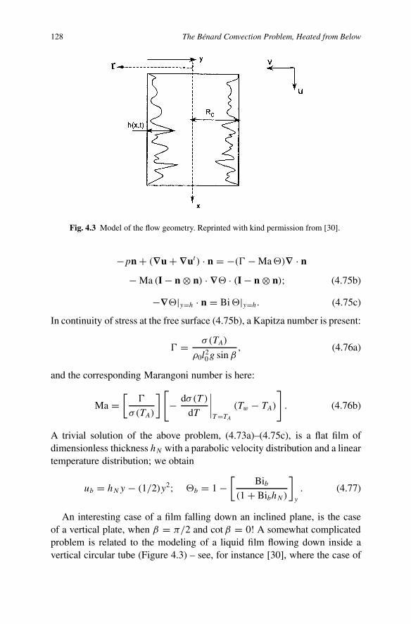
128 The Bénard Convection Problem, Heated from Below
Fig. 4.3 Model of the flow geometry. Reprinted with kind permission from [30].
−pn + (∇u + ∇ut ) · n = −(� − Ma�)∇ · n
− Ma (I − n ⊗ n) · ∇� · (I − n ⊗ n); (4.75b)
−∇�|y=h · n = Bi�|y=h. (4.75c)
In continuity of stress at the free surface (4.75b), a Kapitza number is present:
� = σ (TA)
ρ0l20g sin β
, (4.76a)
and the corresponding Marangoni number is here:
Ma =[
�
σ(TA)
] [− dσ (T )
dT
∣∣∣∣T=TA
(Tw − TA)
]. (4.76b)
A trivial solution of the above problem, (4.73a)–(4.75c), is a flat film ofdimensionless thickness hN with a parabolic velocity distribution and a lineartemperature distribution; we obtain
ub = hNy − (1/2)y2; �b = 1 −[
Bib(1 + BibhN)
]y
. (4.77)
An interesting case of a film falling down an inclined plane, is the caseof a vertical plate, when β = π/2 and cot β = 0! A somewhat complicatedproblem is related to the modeling of a liquid film flowing down inside avertical circular tube (Figure 4.3) – see, for instance [30], where the case of

Convection in Fluids 129
Fig. 4.4 Steady flow over a single sharp step down in topography. Reprinted with kind per-mission from [31].
a high Reynolds number Re is considered, in order to make a more realisticcomparison with the experimental data. In [30], δ is the ratio between thefilm thickness and the characteristic length related to ∂/∂t ∼ ∂x ∼ δ � 1,and it is assumed that δ Re = O(1). Unfortunately, the liquid is assumedincompressible and the Marangoni effect is absent, only the (large) effect ofthe Weber number (δ2 We = O(1)) is taken into account. On the other hand, alarge number of applications require coating of a liquid film over a substratewith topography (see [31]). Steady one-dimensional flow over coating of aliquid film over a substrate with a one-dimensional feature such as a trench[32] is a prototype problem for more complicated situations such as coatingover two-dimensional features and coating flows driven by complex bodyforces. Kalliadasis et al. [33] performed a parametric study of this problem,based only on lubrication theory. The combined influence of the topographyand the surface tension results in a capillary ridge upstream of the step assketched in Figure 4.4a. Flow over a planar substrate, with a portion of thesurface heated by the temperature profil T (x), showing a dip and a ridge assketched in Figure 4.4b.
In a short note by Limat [34], instability of a liquid hanging below a solidceiling (see Figure 4.5) is considered. According to the author, depending

130 The Bénard Convection Problem, Heated from Below
Fig. 4.5 Studied geometry. Reprinted with kind permission from [23].
on the value of the ratio lc/lv (lc = (σ/ρg)1/2 and lv = (µ2/gρ2)1/3 twodifferent behaviors (inviscid or viscous) can be observed.
For a given liquid layer, varying the (finite) thickness h is equivalent toexploring three domains following a straight line whose position depends onlc/ lv.
For lc � lv, one will observe the successive states (thin-viscous, finite-inviscid, semi-infinite-inviscid) and for lc � lv (thin-viscous, finite-viscous,semi-infinite-viscous) we observe that the considered instability is relatedto a Rayleigh–Taylor instability which occurs whenever fluids of differentdensity are subject to acceleration in a direction opposite that of the densitygradient (see a review by Sharp in [35]).
Finally, the reader can find in [18] a general formulation for a three-dimensional thin film (subject to van der Waals forces, surface tension, andsurfactants) using a curvilinear coordinate system which is defined by thepositions of the interfaces (free-free case) of the film; note that a long-waveapproximation is used. For practical application, the authors consider a pla-nar, spherical, and cylindrical thin free film, and a bounded film in the formof a catenoid (which is a very straightforward bounded film case – the simpleconfining geometry giving rise to an uncomplicated set of boundary condi-tions).
In Chapter 10 the reader can find a discussion and references related tovarious liquid film problems.
References
1. H. Bénard, Les tourbillons cellulaires dans une nappe liquide. Revue Générale des Sci-ences Pures et Appliquées 11, 1261–1271 and 1309–1328, 1900. See also: Les tour-billons cellulaires dans une nappe liquide transportant de la chaleur par convection enrégime permanent. Annales de Chimie et de Physique 23, 62–144, 1901.

Convection in Fluids 131
2. S. Chandrasekhar, Hydrodynamic and Hydromagnetic Stability. Clarendon Press, Ox-ford, 1961. See also: Dover Publications, New York, 1981.
3. E.L. Koschmieder, Bénard Cells and Taylor Vortices. Cambridge University Press, Cam-bridge, 1993.
4. C. Marangoni, Sull’espansione delle gocce di un liquido gallegianti sulla superficie di al-tro liquido. Pavia: Tipografia dei fratelli Fusi, 1965 and Ann. Phys. Chem. (Poggendotff)143, 337–354, 1871.
5. J. Plateau, Statique Experimentale et Theorique des Liquides Soumis aux Seules ForcesMoléculaires, Vol. 1. Gauthier-Villars, Paris, 1873.
6. R.Kh. Zeytounian, The Bénard–Marangoni thermocapillary-instability problem.Physics-Uspekhi 41(3), 241–267, March 1998 [English edition].
7. D.A. Nield, Surface tension and buoyancy effects in cellular convection. J. Fluid Mech.19, 341–352, 1964.
8. M.J. Block, Surface tension as the cause of Bénard cells and surface deformation in aliquid film. Nature 178, 650–651, 1956.
9. R.Kh. Zeytounian, The Bénard–Marangoni thermocapillary instability problem: On therole of the buoyancy. Int. J. Engng. Sci. 35(5), 455–466, 1997.
10. M.G. Velarde and R.Kh. Zeytounian (Eds.), Interfacial Phenomena and the MarangoniEffect. CISM Courses and Lectures, No. 428, Udine. Springer-Verlag, Wien/New York,2002.
11. S.H. Davis, Thermocapillary instabilities. Ann. Rev. Fluid Mech. 19, 403–435, 1987.12. J.R.A. Pearson, On convection cells induced by surface tension. J. Fluid Mech. 4, 489–
500, 1958.13. S.J. Vanhook et al., Long-wavelength instability in surface-tension-driven Bénard con-
vection. Phys. Rev. Lett. 75, 4397, 1995.14. D.D. Joseph, Stability of Fluid Motions, Vol. II. Springer, Heidelberg, 1976.15. P.M. Parmentier, V.C. Regnier and G. Lebond, Nonlinear analysis of coupled gravita-
tional and capillary thermoconvection in thin fluid layers. Phys. Rev. E 54(1), 411–423,1996.
16. M. Takashima, J. Phys. Soc. Japan 50(8), 2745–2750 and 2751–2756, 1980.17. R.Kh. Zeytounian, Int. J. Engng. Sci. 27(11), 1361, 1989.18. M.P. Ida and M.J. Miksis, The dynamics of thin films. I. General theory; II. Applications.
SIAM J. Appl. Math. 58(2), 456–473 (I) and 474–500 (II), 1998.19. D.J. Needham and J.H. Merkin, J. Fluid Mech. 184, 357–379, 1987.20. Ch. Bailly, Modélisation asymptotique et numérique de l’écoulement dû à des disques
en rotation. Thesis, Université de Lille I, Villeneuve d’Ascq, No. 1512, 160 pp., 1995.21. D.D. Joseph and Yu.R. Renardy, Fundamentals of Two-Fluid Dynamics. Part I: Mathe-
matical Theory and Applications. Springer-Verlag, 1993.22. C. Ruyer-Quil, B. Scheid, S. Kalliadasis, M.G. Velarde and R.Kh. Zeytounian, Thermo-
capillary long-waves in a liquid film flow. Part 1: Low-dimensional formulation. J. FluidMech. 538, 199–222, 2005.
23. A. Oron, S.H. Davis and S.G. Bankoff, Long-scale evolution of thin liquid film. Rev.Modern Phys. 69(3), 931–980, July 1997.
24. J.K. Platten and J.C. Legros, Convection in Liquids, 1st edn. Springer-Verlag, Berlin,1984.
25. B. Scheid, C. Ruyer-Quil, S. Kalliadasis, M.G. Velarde and R.Kh. Zeytounian, Thermo-capillary long-waves in a liquid film flow. Part 2: Linear stability and nonlinear waves.J. Fluid Mech. 538, 223–244, 2005.
26. D. Dowson, History of Tribology. Longmans, Green, London/New York, 1979.

132 The Bénard Convection Problem, Heated from Below
27. H. Schlichting, Boundary-Layer Theory. McGraw-Hill, New York, 1968.28. C.-S. Yih, Stability of parallel laminar flow down an inclined plane. Phys. Fluids 6, 321–
333, 1963.29. T.B. Benjamin, Wave formation in laminar flow down an inclined plane. J. Fluid Mech.
2, 554–574, 1957.30. S. Ndoumbe, F. Lusseyran, B. Izrar, Contribution to the modeling of a liquid film flowing
down inside a vertical circular tube. C.R. Mecanique 331, 173–178, 2003.31. C.M. Gramlich, S. Kalliadasis, G.M. Homsy and C. Messer, Optimal leveling of flow
over one-dimensional topography by Marangoni stresses. Phys. Fluids 14(6), 1841–1850, June 2002.
32. L.E. Stillwagon and R.G. Larson, Leveling of thin film over uneven substrates duringspin coating. Phys. Fluids A2, 1937, 1990.
33. S. Kalliadasis, C. Bielarz, and G.M. Homsy, Steady free-surface thin film flows overtopography. Phys. Fluids 12, 1889, 2000.
34. L. Limat, Instability of a liquid hanging below a solid ceiling: influence of layer thick-ness. C.R. Acad. Sci. Paris, Ser. II 317, 563–568, 1993.
35. D.H. Sharp, Physica D 12, 3–18, 1984.

Chapter 5The Rayleigh–Bénard Shallow ThermalConvection Problem
5.1 Introduction
It is usual in the literature (see, for instance, the book by Drazin and Reid [1])to denote as Rayleigh–Bénard (RB) shallow thermal convection, the instabil-ity problem produced mainly by buoyancy, possibly including the Marangoniand Biot effects in a non-deformable free surface.
In Chapter4, all the material necessary for a rational derivation of the RBequations governing model shallow thermal convection is in fact preparedfor obtaining such a result via the Boussinesq limiting process written belowin (5.3a). Namely, if we choose to focus on three unknown dimensionlessfunctions
u′(t ′, x′, y′, z′), (5.1a)
� = [T (t ′, x′, y′, z′)− TA]/(Tw − TA), (5.1b)
π(t ′, x′, y′, z′) =(
1
Fr2d
) {[(p − pA)
gdρd
]+ z′ − 1′
}, (5.1c)
and consider our two main small parameters to be
ε′ = α(TA)(Tw − TA) ≡ −[(Tw − TA)
ρ(TA)
] (dρ(T )
dT
)A
, (5.2a)
Fr2d = (ν(TA)/d)
2
gd, (5.2b)
related to a weakly expansible liquid
α(TA) = −(
1
ρ(TA)
)(dρ(T )
dT
)A
� 1, (5.2c)
133
134 The Rayleigh–Bénard Shallow Thermal Convection Problem
and with a not very thin liquid layer
Fr2d � 1 ⇒ d �
(ν2A
g
)1/3
, (5.2d)
then it is necessary to take into account the following Boussinesq limitingprocess:
ε′ ↓ 0 and Fr2d ↓ 0 such that Gr = ε′
Fr2d
= O(1), (5.3a)
the Grashof number Gr being a fixed reference parameter, associated withthe asymptotic expansion relative to ε:
u′ = uRB + ε′u1 + · · · ,� = �RB + ε′�1 + · · · ,π = πRB + ε′π1 + · · · . (5.3b)
The dominant dimensionless equations and boundary conditions at z′ = 0and z′ = H ′(t ′, x′, y′), for u′, � and π , governing (with an error of ε′2) theexact Bénard problem, heated from below, with an upper, deformable freesurface subject to Newton’s cooling law, are the following:
∇′ · u′ = ε′ d�dt ′
; (5.4a)
[1 − ε′�]du′
dt ′+ ∇′π −
(ε′
Fr2d
) [�−
(1
K0
)ε′(1 − z′)
]k
= ∇′u′ + (1/3)ε′∇′(
d�
dt ′
); (5.4b)
[1 − ε′Bd�]d�
dt ′− ε′Bo′
[Td
(Tw − TA)+�
] [Fr2
d
dπ ′
dt ′− u′
3
]
=(
1
Pr
)∇′�+ (1/2 Gr)ε′Bo′
[∂u′
i
∂x′j
+ ∂u′j
∂x′i
]2
− ε′(
1
Pr
)DA
∂
∂x′j
(�∂�
∂x′j
), (5.4c)

Convection in Fluids 135
u′ = 0
� = 1
}at z′ = 0; (5.5)
u′3 = ∂H ′
∂t ′+ u′
1∂H ′
∂x′ + u′2∂H ′
∂y′ , at z′ = H ′(t ′, x′, y′); (5.6a)
π = [H ′(t ′, x′, y′) − 1]Fr2
d
+(
∂u′i
∂x′j
+ ∂u′j
∂x′i
)n′
in′j − (2/3)ε′ d�
dt ′,
+ (We − Ma �)(∇′‖ · n′), at z′ = H ′(t ′, x′, y′); (5.6b)
(∂u′
i
∂x′j
+ ∂u′j
∂x′i
)t′(k)i n′
j + Ma t′(k)i
∂�
∂x′i
= 0, k = 1 and 2,
at z′ = H ′(t ′, x′, y′); (5.6c)
(1 − ε′DA)∂�
∂n′ + Biconv� = 0, at z′ = H ′(t ′, x′, y′); (5.6d)
and
H ′(t ′, x′, y′) = H
d≡ 1 + ηh′(t ′, x′, y′).
During the Boussinesq limiting process (5.3a), the constant parameters1/K0, Bd , DA, and Prandtl (Pr), Biot (Biconv), Marangoni,
Ma =[−dσ (T )
dT
]A
d(Tw − TA)
ρAν2A
(5.7a)
with
σ (T ) = σ (TA) −[−dσ (T )
dT
]A
(T − TA), (5.7b)
and Boussinesq
Bo′ = gd
(Tw − TA)CpA
(5.7c)
numbers are fixed, O(1).The Weber number
We = σAd
ρAν2A
, (5.7d)
which is usually large, is assumed such that
η We = We∗ = O(1), (5.8)

136 The Rayleigh–Bénard Shallow Thermal Convection Problem
according to the third term in upper condition (5.6c) for π because we wantto take into account the effect of the Weber number.
We observe that the free surface amplitude parameter η is necessarilya small parameter because, in the upper, free-surface condition for π , thesquare of the Froude number Fr2
d � 1, and as a consequence we assume thefollowing similarity rule between η and Fr2
d :
η
Fr2d
= η∗ = O(1), when η ↓ 0 and Fr2d ↓ 0. (5.9)
After the above mise en scène, in this chapter, the next ‘tricky step’ is tofirst extract from the above information, (5.1a) to (5.9), via the Boussinesqlimiting process (5.3a), associated with the asymptotic expansion (5.3b), aconsistent Rayleigh–Bénard model problem for the leading-order functions,uRB, �RB and πRB. Then, a second-order, linear, model problem, a compan-ion to the leading-order RB model, must be derived.
We observe again that the way described above is the only consistent onefor a rational derivation of the RB model and, associated with this RB model,a second-order model for u1, �1 and π1, according to asymptotic expansion(5.3b).
The rational approach is adopted here to make sure that, terms neglected,in leading and second-order model equations, are really much smaller thanthose retained. Until this is done, and even now it is possible in part, it willbe difficult to convince the detached and possibly skeptical reader of theirvalue as an aid to understanding and in various applications.
A second, important from my point of view, observation, concerns the roleof the squared Froude number (5.2b) in the rational process which gives theopportunity to derive successfully the RB or BM model problems in accor-dance with the value of the thickness d of the liquid layer. Namely, for theRB model problem, as Fr2
d � 1, then (5.2d) is valid and gives for d a lowerbound (dRB � 1 mm) which strongly depends on the kinematic viscosityν(TA). However, for this RB model problem, where the viscous dissipationis excluded because Bo′ ≈ 1, we obtain also an upper bound for the thicknessd of the liquid layer; namely from (5.7c),
d ≈ (Tw − TA)
(g/CpA), (5.10)
and we observe that the value of the thickness d of the liquid layer is alsostrongly dependent on the temperature difference (Tw − TA).
In the above mathematical formulation of the classical Bénard thermal-free surface, heated from below, problem, issuing from the unsteady NS–F

Convection in Fluids 137
full problem, there are two mechanisms responsible for driving the convec-tive instability:
• the first one is (in equation (5.4b)) the density variation generated by thethermal (weak) expansion of the liquid (effect of the Grashof numberGr);
• the second results from the free surface tension gradients (in upper con-ditions (5.6c) and (5.6c), an effect of the Marangoni number Ma) due totemperature dependence of the surface tension at the upper, free surfaceof the liquid layer.
We also observe that the non-deformable free-surface condition (5.6c), forthe dimensionless pressure π , is (asymptotically) only consistent under thecondition (5.9), which, in fact, ‘smoothes out’ the deformations of the upper,free surface!
In derivation of the RB shallow convection model problem it is necessary,in reality, to consider three similarity rules, between the small parameters η,ε′, Fr2
d and large parameter We, when
η → 0, ε′ → 0, Fr2 → 0, and We → ∞, (5.11a)
such thatη
Fr2= η∗, Gr = ε′
Fr2d
, ηWe = We∗, (5.11b)
where η∗, Gr and We∗ are all O(1).With (5.11a, b), we observe also that for the value of the purely static basic
dimensionless temperature gradients βs – given in (4.39) and linked with theBénard conduction effect – we have the relation
βs =(CpA
g
) [Bis
1 + Bis
], (5.12)
when we replace (Tw − TA)/d by CpA/g according to (5.10). Relation(5.12) exhibits the dependence of the purely static motionless (in conductionregime) basic temperature gradient βs from the specific heat of the liquidCpA, at constant pressure and constant temperature TA.
From the similarity rule ηWe ≈ 1, with (5.7d) and the similarity rule(5.9), we can also write the following upper bound (instead of (5.10)) for thethickness d of the liquid layer:
d ≈[σA
gρA
]1/2
(5.13)

138 The Rayleigh–Bénard Shallow Thermal Convection Problem
and, instead of (5.10), we write in such a case a relation for the temperaturedifference (Tw − TA):
(Tw − TA) ≈ gd
CpA
. (5.14)
Thus the above relations (5.2d), (5.12), (5.13) and (5.14), written for the dataβs , d and (Tw −TA) give some criteria related to various physical parameterscharacterizing the weakly expansible liquid layer.
5.2 The Rayleigh–Bénard System of Model Equations
Now, the application of the Boussinesq limiting process (5.3a), with as-ymptotic expansion (5.3b), gives for the leading-order RB three functions:uRB, �RB and πRB, in (5.3b), the following Rayleigh–Bénard system of threemodel equations (the terms with ε are neglected):
∇′ · uRB = 0; (5.15a)
duRB
dt ′+ ∇′πRB − Gr�RBk = �′uRB; (5.15b)
d�RB
dt ′=
(1
Pr
)�′�RB, (5.15c)
where
d
dt ′= ∂
∂t ′+ (uRB · ∇′)
= ∂
∂t ′+ u1RB
∂
∂x′ + u2RB∂
∂y′ + u3RB∂
∂z′ . (5.16)
From (5.6a–d) – see also, for instance, our discussion in Section 4.3 – for theabove model equations (5.15a–c), in the leading order (again the terms withε being neglected), we derive the associated upper boundary conditions at anon-deformable free surface z′ = 1, when we take into account the similarityrule (5.11) and the results of Section 4.3. First, with (4.31a),
uRB · k ≡ u3RB = 0, at z′ = 1, (5.17a)
according to (5.6a), and then from (5.6c), with (4.31e–f), we derive the fol-lowing two conditions:
Ma∂�RB
∂x′ = −[∂u1RB
∂z′ + ∂u3RB
∂x′
], at z′ = 1, (5.17b)

Convection in Fluids 139
and
Ma∂�RB
∂y′ = −[∂u2RB
∂z′ + ∂u3RB
∂y′
], at z′ = 1. (5.17c)
But equation (5.15a) gives
−∂[∂u1RB/∂x′ + ∂u2RB/∂y
′]∂z′ = ∂2u3RB
∂z′2 , at z′ = 1,
and, instead of (5.17b, c), with (5.17a), we obtain the following single, uppercondition at a non-deformable free surface:
∂2u3RB
∂z′2 = Ma
[∂2�RB
∂x′2 + ∂2�RB
∂y′2
], at z′ = 1. (5.17d)
Finally, from (5.6d), when we take into account the smallness of the ampli-tude parameter η, we derive a condition for �:
∂�RB
∂z′ + Biconv �RB = 0, at z′ = 1. (5.17e)
The upper conditions (5.17a), (5.17d) and (5.17e), with the boundary condi-tions at lower plate
u1RB = u2RB = u3RB = 0 and �RB = 1, at z′ = 0, (5.18)
are the associated boundary conditions for the RB, ‘rigid-free’ model equa-tions (5.15a–c). The upper condition (5.17e) for the dimensionless temper-ature �RB, defined by (5.1b), is used in two recent papers [2, 3]. The RBmodel problem formulated there, (5.15a–c)–(5.17a, d, e), being relative to a‘rigid-free’ case, is a sequel of the Bénard physical starting problem, heatedfrom below, when we take into account the existence of a deformable upper,free surface.
The ‘rigid-rigid’ case, has been considered, in fact without the Marangoniand Biot effects, in Chapter 3 devoted to Rayleigh’s 1916 problem; see, forinstance, the model problem (3.25a–d) derived in Section 3.4.
Often a ‘free-free’, ‘unrealistic’, case is also considered when the corre-sponding boundary conditions (again, without the Marangoni and Biot ef-fects) are
u3RB = 0 and∂2u3RB
∂z′2 = 0, at both free boundaries, z′ = 0, 1, (5.19a)
∂�
∂z′ = 0, at z′ = 0, 1, (5.19b)

140 The Rayleigh–Bénard Shallow Thermal Convection Problem
when the boundaries z′ = 0 and z′ = 1 are modelled as a perfect insulator(as is the case in [4]) or, if the boundaries are at fixed temperature:
� = 1, at z′ = 0, z′ = 1. (5.19c)
In most cases (in the ad hoc approaches), as a ‘free-free’ RB problem, thefollowing dimensionless equations are considered:
∇ · V = 0; (5.20a)(
1
Pr
)dV
dt= −∇�+ T k + ∇2V; (5.20b)
dT
dt= Raw + ∇2T , (5.20c)
with Ra (= Pr Gr) the Rayleigh number, for the dimensionless velocity vec-tor V, pressure � and temperature T , with as boundary conditions
T = w = 0,∂2w
∂z2= 0 at z = 0, z = 1. (5.20d)
In equation (5.20c) and boundary conditions (5.20d),
w = V · k. (5.20e)
Above, in the derivation of the RB, free-free, model problem (5.15a–c)–(5.17a, d, e), we have not considered the upper condition (5.6c) for π ! Itis however true that from this upper condition (5.6c) we have concluded thesmallness of the amplitude parameter η (see (5.9)).
Indeed, this upper condition (5.6c) gives an equation for the determina-tion of the deformation h′(x′, y′) of the free surface, when we take into ac-count the similarity rule (5.8). Namely, we have aready noted in Section 1.2(see, for instance, equation (1.28a)), the emergence of such an equation forh′(x′, y′) from the upper jump condition, for the dimensionless pressure π .
It seems that such an equation for the deformation of the free surface hadnot been discovered before! Here, in the framework of our rational analy-sis and asymptotic modelling approach, such a result is expected and is ob-tained from (5.6c), when we take into account (4.31g) and the similarityrule (5.8). This equation is written in the following form for the deformationh′(t ′, x′, y′) of the upper, free surface:
∂2h′
∂x′2 + ∂2h′
∂y′2 −(η∗
We∗
)h′ = −
(1
We∗
)π(t ′, x′, y′, z′ = 1). (5.21)

Convection in Fluids 141
Fig. 5.1 Two ‘almost regular’ RB convection patterns. Reprinted with kind permission from[10].
Fig. 5.2 Two ‘exotic’ RB convection patterns. Reprinted with kind permission from [10].
In Figures 5.1–5.3, some ‘spectacular’ RB convection patterns selectedfrom the cited survey paper [10] are presented.
The linear theory of the RB shallow convection model problem is verywell analyzed in the Drazin and Reid book [1], and also in Chandrasekhar’smonograph [5]. The RB thermal convection, governed by the above modelproblem (5.15a–c)–(5.17a, d, e), represents, when Ma and Bi effects are ne-glected, the simplest (but very ‘rich’) example of hydrodynamic instabilityand transition to turbulence in a fluid system. In this case (as Ma = 0 andBi = 0), the more important effect is linked with buoyancy (Archimedean
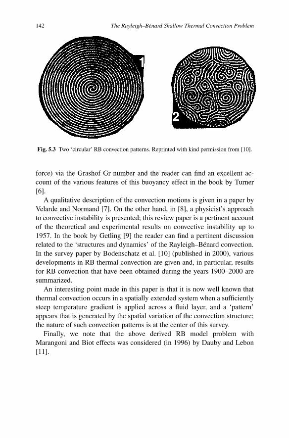
142 The Rayleigh–Bénard Shallow Thermal Convection Problem
Fig. 5.3 Two ‘circular’ RB convection patterns. Reprinted with kind permission from [10].
force) via the Grashof Gr number and the reader can find an excellent ac-count of the various features of this buoyancy effect in the book by Turner[6].
A qualitative description of the convection motions is given in a paper byVelarde and Normand [7]. On the other hand, in [8], a physicist’s approachto convective instability is presented; this review paper is a pertinent accountof the theoretical and experimental results on convective instability up to1957. In the book by Getling [9] the reader can find a pertinent discussionrelated to the ‘structures and dynamics’ of the Rayleigh–Bénard convection.In the survey paper by Bodenschatz et al. [10] (published in 2000), variousdevelopments in RB thermal convection are given and, in particular, resultsfor RB convection that have been obtained during the years 1900–2000 aresummarized.
An interesting point made in this paper is that it is now well known thatthermal convection occurs in a spatially extended system when a sufficientlysteep temperature gradient is applied across a fluid layer, and a ‘pattern’appears that is generated by the spatial variation of the convection structure;the nature of such convection patterns is at the center of this survey.
Finally, we note that the above derived RB model problem withMarangoni and Biot effects was considered (in 1996) by Dauby and Lebon[11].
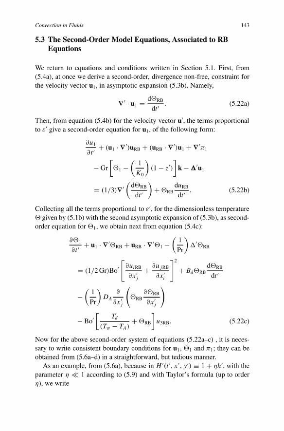
Convection in Fluids 143
5.3 The Second-Order Model Equations, Associated to RBEquations
We return to equations and conditions written in Section 5.1. First, from(5.4a), at once we derive a second-order, divergence non-free, constraint forthe velocity vector u1, in asymptotic expansion (5.3b). Namely,
∇′ · u1 = d�RB
dt ′. (5.22a)
Then, from equation (5.4b) for the velocity vector u′, the terms proportionalto ε′ give a second-order equation for u1, of the following form:
∂u1
∂t ′+ (u1 · ∇′)uRB + (uRB · ∇′)u1 + ∇′π1
− Gr
[�1 −
(1
K0
)(1 − z′)
]k − �′u1
= (1/3)∇′(
d�RB
dt ′
)+ �RB
duRB
dt ′. (5.22b)
Collecting all the terms proportional to ε′, for the dimensionless temperature� given by (5.1b) with the second asymptotic expansion of (5.3b), as second-order equation for �1, we obtain next from equation (5.4c):
∂�1
∂t ′+ u1 · ∇′�RB + uRB · ∇′�1 −
(1
Pr
)�′�RB
= (1/2 Gr)Bo′[
∂uiRB
∂x′j
+ ∂ujRB
∂x′i
]2
+ Bd�RBd�RB
dt ′
−(
1
Pr
)DA
∂
∂x′j
(�RB
∂�RB
∂x′j
)
− Bo′[
Td
(Tw − TA)+ �RB
]u3RB. (5.22c)
Now for the above second-order system of equations (5.22a–c) , it is neces-sary to write consistent boundary conditions for u1, �1 and π1; they can beobtained from (5.6a–d) in a straightforward, but tedious manner.
As an example, from (5.6a), because in H ′(t ′, x′, y′) ≡ 1 + ηh′, with theparameter η � 1 according to (5.9) and with Taylor’s formula (up to orderη), we write
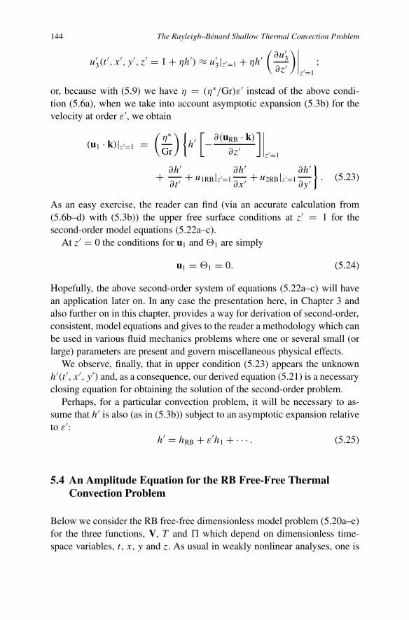
144 The Rayleigh–Bénard Shallow Thermal Convection Problem
u′3(t
′, x′, y′, z′ = 1 + ηh′) ≈ u′3|z′=1 + ηh′
(∂u′
3
∂z′
)∣∣∣∣z′=1
;
or, because with (5.9) we have η = (η∗/Gr)ε′ instead of the above condi-tion (5.6a), when we take into account asymptotic expansion (5.3b) for thevelocity at order ε′, we obtain
(u1 · k)|z′=1 =(
η∗
Gr
){h′
[−∂(uRB · k)
∂z′
]∣∣∣∣z′=1
+ ∂h′
∂t ′+ u1RB|z′=1
∂h′
∂x′ + u2RB|z′=1∂h′
∂y′
}. (5.23)
As an easy exercise, the reader can find (via an accurate calculation from(5.6b–d) with (5.3b)) the upper free surface conditions at z′ = 1 for thesecond-order model equations (5.22a–c).
At z′ = 0 the conditions for u1 and �1 are simply
u1 = �1 = 0. (5.24)
Hopefully, the above second-order system of equations (5.22a–c) will havean application later on. In any case the presentation here, in Chapter 3 andalso further on in this chapter, provides a way for derivation of second-order,consistent, model equations and gives to the reader a methodology which canbe used in various fluid mechanics problems where one or several small (orlarge) parameters are present and govern miscellaneous physical effects.
We observe, finally, that in upper condition (5.23) appears the unknownh′(t ′, x′, y′) and, as a consequence, our derived equation (5.21) is a necessaryclosing equation for obtaining the solution of the second-order problem.
Perhaps, for a particular convection problem, it will be necessary to as-sume that h′ is also (as in (5.3b)) subject to an asymptotic expansion relativeto ε′:
h′ = hRB + ε′h1 + · · · . (5.25)
5.4 An Amplitude Equation for the RB Free-Free ThermalConvection Problem
Below we consider the RB free-free dimensionless model problem (5.20a–e)for the three functions, V, T and � which depend on dimensionless time-space variables, t , x, y and z. As usual in weakly nonlinear analyses, one is

Convection in Fluids 145
constrained to values of the Ra close to critical Rayleigh Rac, and a ‘super-criticality’ parameter r, of order O(1), is introduced such that
Ra = Rac + κ2r, (5.26a)
with κ � 1 regarded as a measure of the closeness Ra from Rac.In the free-free case the RB system first becomes unstable when
Rac = 27π4
4, (5.26b)
where from a periodic array of convection rolls arises a critical wave number
kc = π√2. (5.26c)
First it is necessary to introduce the slow scales
ξ = κx, η = κ1/2y, τ = κ2t. (5.27a)
The choice (5.27a) of slow scales is motivated by the behavior of the lin-ear growth rate in the vicinity of (kc,Rac), and by the expected form ofthe leading-order nonlinearity in the final amplitude equation. All dependentvariables are expanded according to
(u, v,w,�, T ) ≡ U = κU1 + κ3/2U3/2 + κ2U2
+ κ5/2U5/2 + κ3U3 + · · · . (5.27b)
where
Un = U(0)n (ξ, η, τ, z)+ Real[�U(m)
n (ξ, η, τ, z) exp(imkcx)], (5.27c)
with m = 1 to N and n = 1 + (p/2), p = 0, 1, 2, 4, . . . .In Zeytounian’s book [12, pp. 378–392], the reader can find a detailed
derivation of an amplitude evolution equation. Namely, for the amplitudeA(ξ, η, τ) of the O(κ) problem (see (5.28a)). We give below only the mainsteps of this asymptotic derivation.
The first step is substitution of the above expansion (5.27c) into the gov-erning RB equations (5.20a–c) and boundary conditions (5.20d), after intro-ducing (5.26a) and the slow scales (5.27a).
Because U(0)1 = 0, describing the periodic array of convection rolls, the
solution of the O(κ) problem (n = 1, m = 1) for U(1)1 is obtained in the
following form:
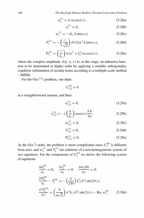
146 The Rayleigh–Bénard Shallow Thermal Convection Problem
u(1)1 = πA cos(πz), (5.28a)
v(1)1 = 0, (5.28b)
w(1)1 = −ikcA sin(πz), (5.28c)
T(1)
1 = −(
i√2
)(9/2)π3A sin(πz), (5.28d)
�(1)1 =
(i
kc
)π(π2 + k2
c )A cos(πz), (5.28e)
where the complex amplitude A(ξ, η, τ) is, at this stage, an unknown func-tion to be determined at higher order by applying a suitable orthogonalitycondition (elimination of secular terms according to a multiple-scale method– MSM).
For the O(κ3/2) problem, one finds
U(0)3/2 = 0
in a straightforward manner, and then:
u(1)3/2 = 0, (5.29a)
v(1)3/2 = −i
(π
kc
)cos(πz)
∂A
∂η, (5.29b)
w(1)3/2 = 0, (5.29c)
T(1)
3/2 = 0, (5.29d)
�(1)3/2 = 0. (5.29e)
At the O(κ2) order, the problem is more complicated since U(0)2 is different
from zero, and w(1)2 and T (1)
2 are solutions of a non-homogeneous system oftwo equations. For the components of U(0)
2 we derive the following systemof equations:
∂u(0)2
∂z= 0,
∂v(0)2
∂z= 0,
∂w2(0)
∂z= 0,
∂�(0)2
∂z− T
(0)2 = −
( π
2 Pr
)k2c |A2| sin(2πz),
∂2T(0)
2
∂z2=
(9
4√
2
)π4kc|A2| sin(2πz)− Rac w
(0)2 . (5.30a)

Convection in Fluids 147
The solution of (5.30a) is simply:
u(0)2 = 0, v
(0)2 = 0, w
(0)2 = 0,
T(0)
2 = −(9/32)π3|A2| sin(2πz),
�(0)2 = (1/8)
[(1
Pr
)+ (9/8)
]π2|A2| cos(2πz). (5.30b)
For the components of U(1)2 , we obtain first
v(1)2 = 0, (5.30c)
and then for the two functions w(1)2 and T
(1)2 we derive again a non-
homogeneous system of two equations, namely:
(∂2
∂z2− k2
c
)w(1)2 − k2
c T(1)
2 = F2, (5.30d)
(∂2
∂z2− k2
c
)T(1)
2 + Rac w(1)2 = G2, (5.30e)
where
F2 = −(3/2)π4
[∂A
∂ξ−
(i
2kc
)∂2A
∂η2
]sin(πz), (5.30f)
G2 = −(9/2)π4
[∂A
∂ξ−
(i
2kc
)∂2A
∂η2
]sin(πz), (5.30g)
with the boundary conditions
w(1)2 = ∂2w
(1)2
∂z2= T
(1)2 = 0 at z = 0 and 1. (5.30h)
In order for this above problem (5.30d–h) to admit a non-trivial solution,the forcing terms (5.30f, g) must be orthogonal to the adjoint eigenfunc-tions of the homogeneous problem, i.e., to the adjoint eigenfunctions of theequations at order O(κ) with boundary conditions similar to the above (butwritten for w(1)
1 and T (1)1 ). One readily obtains the adjoint eigenfunctions to
be w∗ = −3 sin(πz), and T ∗ = sin(πz), and the othogonality condition isthe following: ∫ 1
0[F2w
∗ +G2T∗] dz = 0, (5.30i)
which is identically satisfied.

148 The Rayleigh–Bénard Shallow Thermal Convection Problem
Then, the solution for w(1)2 and T (1)
2 is
w(1)2 = 0, (5.30j)
T(1)
2 = 3π2
[∂A
∂ξ−
(i
2kc
)∂2A
∂η2
]sin(πz), (5.30k)
and for u(1)2 and �(1)2 , we have:
u(1)2 = −
(π
ikc
)[∂A
∂ξ+
(1
ikc
)∂2A
∂η2
]cos(πz), (5.30l)
�(1)2 = i
(π
kc
)3 [2ikc
∂A
∂ξ+ ∂2A
∂η2
]cos(πz). (5.30m)
At the O(κ5/2) order, all field variables admit a solution of the form (5.27c)with p = 3 and m = 1, and in this case we obtain easily the followingsolution for the components of U(0)
5/2:
u(0)5/2 = 0, (5.31a)
v(0)5/2 = −(3/32)
[(1
Pr
)+ 3/8
]∂|A2|∂η
cos(2πz), (5.31b)
w(0)5/2 = 0, (5.31c)
T(0)
5/2 = 0. (5.31d)
Then for the components of U(1)5/2 we obtain:
u(1)5/2 = 0, (5.31e)
v(1)5/2 =
(4
π
)∂
∂η
[∂A
∂ξ−
(i
2kc
)∂2A
∂η2
]cos(πz), (5.31f)
w(1)5/2 = 0, (5.31g)
T(1)
5/2 = 0. (5.31h)
At the O(κ3) order, all field variables admit a solution of the form (5.27c)with p = 4, m = 1 to 3. However, only the components of U(0)
3 and U(1)3 are
of interest in determining the evolution amplitude equation for the leading-order amplitude A(ξ, η, τ). First, we obtain the following two equations foru(0)3 and w(0)
3 :

Convection in Fluids 149
∂2u(0)3
∂z2= S3, (5.32a)
∂2w(0)3
∂z2= Q3, (5.32b)
where
S3 =(π2
8
)[(1
Pr
)+ 9/8
]∂|A|2∂η
cos(2πz), (5.32c)
Q3 = (3/32)
[(1
Pr
)+ 3/8
]∂|A|2∂η
cos(2πz). (5.32d)
As a consequence, in order to satisfy the boundary conditions
∂u(0)3
∂z= 0, w
(0)3 = 0 at z = 0, 1, (5.32e)
we must enforce the following two compatibility conditions on the forcingterms in (5.32a, b):
∫ 1
0S3 dz = 0,
∫ 1
0Q3 dz = 0, (5.32f)
which are again identically satisfied.Next, forw(1)
3 and T (1)3 we derive a system of two non-homogeneous equa-
tions analogous to the system (5.30d, e) for w(1)2 and T
(1)2 , but with F3 and
G3 on the right-hand side, such that
F3 = 3i
(π3
2√
2
) {(1
Pr
)∂A
∂τ+ ∂2A
∂ξ 2
− (16/3)
[∂A
∂ξ−
(i
2kc
)∂2A
∂η2
]2}
sin(πz), (5.32g)
G3 = −9i
(π3
2√
2
) {∂A
∂τ− ∂2A
∂ξ 2+ (4/3)
[∂A
∂ξ−
(i
2kc
)∂2A
∂η2
]2
−(
2
9π2
)rA−
(π2
8
)cos(2πz)A | A2
}sin(πz). (5.32h)
The boundary conditions are
w(1)3 = ∂2w
(1)3
∂z2= T
(1)3 = 0, at z = 0 and 1. (5.32i)

150 The Rayleigh–Bénard Shallow Thermal Convection Problem
Again, the orthogonality with adjoint eigenfunctions requires that
∫ 1
0[F3w
∗ +G3�∗] dz = 0, (5.32j)
thereby, finally leading to the above evolution equation for the amplitudefunction A(τ, ξ, η), which appears first the solution (5.28a–e) of the O(κ)problem:
[1 +
(1
Pr
)]∂A
∂τ= 4
[∂A
∂ξ−
(i
2kc
)∂2A
∂η2
]2
+(
2
9π2
)rA−
(π2
16
)A|A|2.(5.33)
If
x = 2kcξ, y = 2kcη, t = 16
[1 +
(1
Pr
)]k2c τ, (5.34a)
then for the new amplitude function B(t, x, y), such that
B =(
π
16kc
)A
(x
2kc,y
2kc,
t
16(1 + 1Pr)k
2c
), (5.34b)
the evolution equation for B(t, x, y) takes the final form:
∂B
∂t=
[∂B
∂x− i
∂2B
∂y2
]2
+ µB − B|B|2, (5.35)
withµ =
( r
36π4
).
The reduced amplitude equation (5.35), for B, is the amplitude equation pre-viously derived in 1969 by Newell and Whitehead [13]. Our above derivationof the amplitude equation (5.35) is directly suggested by the paper of Coulletand Huerre [14].
For equation (5.35) we can obtain first a family of stationary periodic (inx) solutions, namely:
Bst = Q exp[iqx), (5.36)
where the amplitude Q is given by the relation
(µ− q2)Q−Q3 = 0 ⇒ Q = (µ− q2)1/2. (5.37)
In order to study the stability of this pattern, we make a change of variables;
B(t, x, y) = [Q+ ρ(t, x, y)] exp[i(qx + ϕ)], (5.38a)

Convection in Fluids 151
with ϕ = ϕ(t, x).In this case, from (5.35) we obtain two equations
∂ρ
∂t= −2Q2ρ − 2ρQ
∂ϕ
∂x+ ∂2
∂x2+ 2q
∂2ρ
∂y2; (5.38b)
∂ϕ
∂t= (2q/Q)
∂ρ
∂x+ ∂2ϕ
∂x2+ 2q
∂2ϕ
∂y2. (5.38c)
Thus the spatial pattern may be subject to two possible modes of perturba-tions. The amplitude mode associated with the variable ρ is governed byequation (5.38b) and in the long-wavelength approximation,
∂
∂x� 1,
∂
∂y� 1,
this amplitude mode is highly damped.By contrast, the remaining variable ϕ corresponds to the marginal phase
mode, its dynamics being governed by equation (5.38c) and, again, in thelong-wavelength limit,
∂ϕ
∂t= 0;
this mode is neutrally stable.To describe the long-wavelength dynamics of the phase mode ϕ, it is le-
gitimate to assume that the amplitude ρ is adiabatically slaved to the slowly-varying phase. To leading order, the amplitude equation (5.38b) can then beapproximated by
ρ ∼ −(q/Q)∂ϕ
∂x, (5.39)
and substituting in (5.38c) gives rise to the phase evolution equation
∂ϕ
∂t=
[1 −
(2q2
Q2
)]∂2ϕ
∂x2+ 2q
∂2ϕ
∂y2, (5.40)
where, according to (5.37),
1 −(
2q2
Q2
)= (µ − 3q2)
(µ − q2)= β. (5.41)
Finally, phase fluctuations are governed by the single diffusive equation
∂ϕ
∂t= β
∂2ϕ
∂x2+ 2q
∂2ϕ
∂x2. (5.42)
ρ

152 The Rayleigh–Bénard Shallow Thermal Convection Problem
The signs of β and q control, respectively, the so-called Eckhaus and zig-zag instability. We note that q can change sign if the basic pattern is zig-zagunstable, and if q > 0, the phase is diffusive in y and no zig-zag instabilitycan take place. If q < 0, the medium is zig-zag unstable and additional termsneed to be brought into equation (5.42) to describe possible two-dimensionalsoliton lattices!
A simplified case for the amplitude evolution equation (5.35), is closelylinked to the assumption that the amplitude B (assumed real) is a functiononly of time t . In such a case we derive from (5.35) the so-called Landau–Stuart equation:
−dB
dt= −
(1
36π4
)rB + B|B|2, (5.43)
where r > 0.
5.5 Instability and Route to Chaos in RB Thermal Convection
We have already noted that the RB thermal convection in a fluid layer heatedfrom below, with a non-deformable upper, free surface and without surfacetension, represents the simplest example of hydrodynamic instability andtransition to turbulence (as a temporal chaos) in a fluid system.
The only systematic analytical method for analyzing the manifold of 3Dnonlinear steady solutions of the RB equations is the perturbation approach(as in Section 5.4) based on the small parameter κ . This approach is partic-ularly appropriate in the case of convection because the instability occurs inthe form of infinitesimal disturbances.
In particular, both evolution amplitude equations (5.35) and (5.43) derivedabove have played an important role in analytical investigations of hydro-dynamic instability in the 60 years from the outset of the so-called ‘finite-dimensional dynamical system approach to turbulence’.
In the framework of this approach, the pioneering role (20 years after Lan-dau’s theory [15]) is ascribed to the Lorenz dynamical system [16], which isa system of three relatively simple ordinary (but nonlinear) differential equa-tions of the following form, for the three amplitude functions of time t , A(t),B(t) and C(t):
dA
dt= −10A + 10B, (5.44a)
dB
dt= −AC + 28A − B, (5.44b)

Convection in Fluids 153
dC
dt= AB − (8/3)C. (5.44c)
Such a Lorenz system (5.44a–c) is derived for the Rayleigh–Bénard two-dimensional problem when, instead of the constraint (5.20a) for the velocityvector V, we consider in the two-dimensional case (∂/∂y ≡ 0 and v ≡ 0) thereduced 2D equation
∂u
∂x+ ∂w
∂z= 0 ⇒ u = ∂ψ
∂z, w = −∂ψ
∂x. (5.45a)
In such a case, after the elimination of �, we derive from (5.20b) for thestream function ψ , the equation
(1
Pr
)[∂∇2ψ
∂t+ D(ψ; ∇2ψ)
]+ ∂T
∂x= ∇2(∇2ψ), (5.45b)
where
D(ψ;f ) = ∂ψ
∂z
∂f
∂x− ∂ψ
∂x
∂f
∂z,
and for temperature T , from (5.20c), we obtain
∂T
∂t+ D(ψ;T ) + Ra
∂ψ
∂x= ∇2T . (5.45c)
According to Lorenz [16], we write the solution of the system of two equa-tions (5.45b, c), for ψ(t, x, z) and T (t, x, z) as
ψ = Pr[A(t) sin
(πx
λ
)sin(πz)
](5.46a)
and
T = Ra[B(t) cos
(πx
λ
)sin(πz) + C(t) sin(2ψz)
]. (5.46b)
The above approximate form (5.46a, b) for ψ and T is compatible with thefollowing boundary conditions (free-free case):
ψ = 0 and∂2ψ
∂z2= 0, T = 0 at z = 0 and z = 1, (5.47a)
ψ = 0 and∂2ψ
∂x2= 0,
∂T
∂x= 0 at x = 0 and x = λ. (5.47b)
Then, by a Galerkin technique, the next step is to substitute the approximate(three amplitudes) solution (5.46a, b), into two 2D equations (5.45b, c), thenrequiring the residue to be orthogonal to each function of the set (5.46a, b).

154 The Rayleigh–Bénard Shallow Thermal Convection Problem
More precisely, after this substitution, on the one hand, the equa-tion obtained from (5.45b) is multipied by sin(pπx/λ) sin(πz) and, onthe other hand, the equation obtained from (5.45c) is multipied bycos(pπx/λ) sin(πz). These two new equations are then integrated over x,between x = 0 and x = λ, and over z, between z = 0 and z = 1. Theseabove two orthogonality conditions with:
(2
π
)∫ π
0sin(iy) sin(jy) dy = δij , (5.48a)
and (2
π
) ∫ π
0cos(iy) sin(jy) dy = δij , (5.48b)
lead to the following system (5.49a) of three equations for the three reduced(see (5.50) time-dependent coefficients X(t), Y (t) and Z(t):
dX
dt= Pr (Y −X),
dY
dt= −XZ + r0X − Y,
dZ
dt= XY − bZ, (5.49a)
with
r0 = Raq2
(π2 + q2)3, (5.49b)
the ‘bifurcation’ parameter.The relation between X(t), Y (t) and Z(t), and the amplitudes A(t), B(t),
C(t) in (5.46a, b) is
X(t) =(πq√
2
)[1
(π2 + q2)
]A(t),
Y (t) = −(
1
Ra
) (πq2
√2
) [1
(π2 + q2)
]B(t),
Z(t) = −(
1
Ra
) [πq2
(π2 + q2)
]C(t). (5.50)
The system (5.49a), with (5.49b), was first obtained by Lorenz [16]. In abook by Sparrow [17] the reader can find a detailed and careful theory of theabove (5.49a) à la Lorenz system. We observe that the condition

Convection in Fluids 155
Fig. 5.4a Lorenz strange attractor – cross-section (A–B) in phase space (A,B,C). Reprintedwith kind permission from [18].
∂
∂X
(dX
dt
)+ ∂
∂Y
(dY
dt
)+ ∂
∂Z
(dZ
dt
)= −[Pr + b + 1] (5.51)
shows that the Lorenz system (5.49a) is real-dissipative!Thanks to system (5.44), Lorenz, in his 1963 paper [16] ‘exhibits’ for
the first time, via a numerical computation of the system (5.44), a ‘strangeattractor’; see Figures 5.4a–c, reproduced from [18, pp. 480–482].
The Lorenz system (5.49a) in a steady state has as constant solution
Xst = ±[b(r0 − 1)], Yst = ±[b(r0 − 1)], Zst = r0 − 1, (5.52a)
r0 − 1 = (Ra − Rac)
Rac. (5.52b)
According to the Routh and Hurwitz criterion, a particular value of r0 (notedr∗
0 ) exists, for which the above steady-state solution (5.52) is unstable – fromthis value for Pr = 10 and b = 8/3 (as in (5.44)) we obtain
r∗0 − 1 = 23.74. (5.53)
As a consequence, a steady-state solution (5.52) of the Lorenz system isunstable when (5.53) is realized. But, because the Lorenz system has no
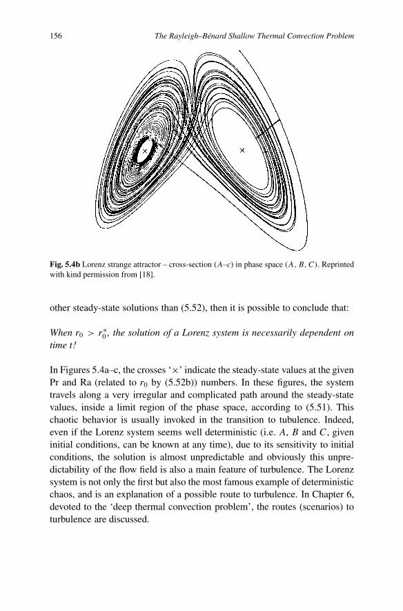
156 The Rayleigh–Bénard Shallow Thermal Convection Problem
Fig. 5.4b Lorenz strange attractor – cross-section (A–c) in phase space (A,B,C). Reprintedwith kind permission from [18].
other steady-state solutions than (5.52), then it is possible to conclude that:
When r0 > r∗0 , the solution of a Lorenz system is necessarily dependent on
time t!
In Figures 5.4a–c, the crosses ‘×’ indicate the steady-state values at the givenPr and Ra (related to r0 by (5.52b)) numbers. In these figures, the systemtravels along a very irregular and complicated path around the steady-statevalues, inside a limit region of the phase space, according to (5.51). Thischaotic behavior is usually invoked in the transition to tubulence. Indeed,even if the Lorenz system seems well deterministic (i.e. A, B and C, giveninitial conditions, can be known at any time), due to its sensitivity to initialconditions, the solution is almost unpredictable and obviously this unpre-dictability of the flow field is also a main feature of turbulence. The Lorenzsystem is not only the first but also the most famous example of deterministicchaos, and is an explanation of a possible route to turbulence. In Chapter 6,devoted to the ‘deep thermal convection problem’, the routes (scenarios) toturbulence are discussed.

Convection in Fluids 157
Fig. 5.4c Lorenz strange attractor – cross-section (B–C) in phase space (A,B,C). Reprintedwith kidn permission from [18].
Finally, we observe that from the Lorenz system (5.49a) it is possible toderive a Landau single equation, e.g., for X(t) when we assume that the twoother amplitudes are independent of time t . Namely, in such a case the firstand third equations of (5.49a) give
Y = X and Z =(
1
b
)X2
and as a consequence , from the second equation (since Y = X and Z =(1/b)X2) of the system (5.49a), for X(t) we obtain
dX
dt= (r0 − 1)X −
(1
b
)X3. (5.54)
Obviously, and unfortunately, this analytic method, a perturbation expansionand a Galerkin technique are of limited usefulness when the Rayleigh num-ber Ra is increased much beyond its critical value. For this case, numericalcomputations have been performed by various authors, e.g., by Curry et al.[20].
Concerning the fully nonlinear, RB convection problem, direct numericalmethods have been used. For this, it is convenient to define five values of
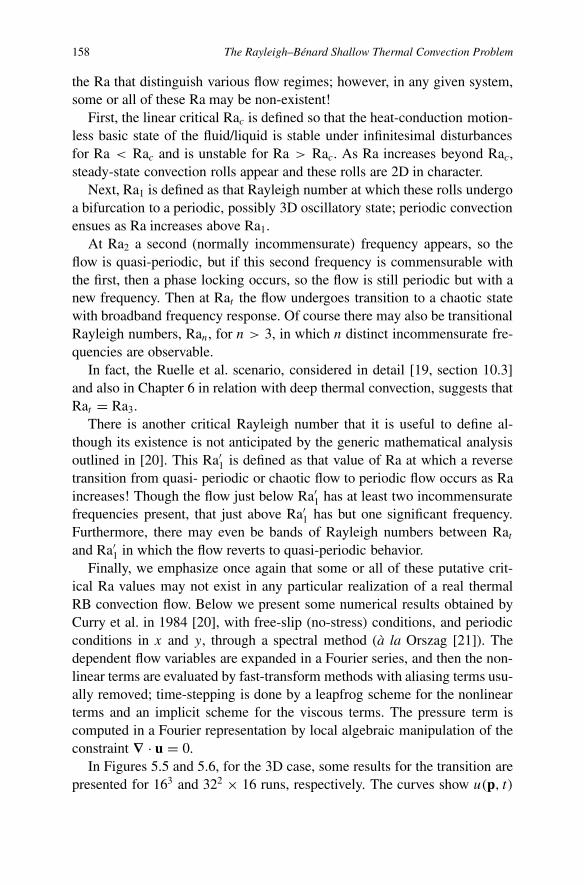
158 The Rayleigh–Bénard Shallow Thermal Convection Problem
the Ra that distinguish various flow regimes; however, in any given system,some or all of these Ra may be non-existent!
First, the linear critical Rac is defined so that the heat-conduction motion-less basic state of the fluid/liquid is stable under infinitesimal disturbancesfor Ra < Rac and is unstable for Ra > Rac. As Ra increases beyond Rac,steady-state convection rolls appear and these rolls are 2D in character.
Next, Ra1 is defined as that Rayleigh number at which these rolls undergoa bifurcation to a periodic, possibly 3D oscillatory state; periodic convectionensues as Ra increases above Ra1.
At Ra2 a second (normally incommensurate) frequency appears, so theflow is quasi-periodic, but if this second frequency is commensurable withthe first, then a phase locking occurs, so the flow is still periodic but with anew frequency. Then at Rat the flow undergoes transition to a chaotic statewith broadband frequency response. Of course there may also be transitionalRayleigh numbers, Ran, for n > 3, in which n distinct incommensurate fre-quencies are observable.
In fact, the Ruelle et al. scenario, considered in detail [19, section 10.3]and also in Chapter 6 in relation with deep thermal convection, suggests thatRat = Ra3.
There is another critical Rayleigh number that it is useful to define al-though its existence is not anticipated by the generic mathematical analysisoutlined in [20]. This Ra′
1 is defined as that value of Ra at which a reversetransition from quasi- periodic or chaotic flow to periodic flow occurs as Raincreases! Though the flow just below Ra′
1 has at least two incommensuratefrequencies present, that just above Ra′
1 has but one significant frequency.Furthermore, there may even be bands of Rayleigh numbers between Ratand Ra′
1 in which the flow reverts to quasi-periodic behavior.Finally, we emphasize once again that some or all of these putative crit-
ical Ra values may not exist in any particular realization of a real thermalRB convection flow. Below we present some numerical results obtained byCurry et al. in 1984 [20], with free-slip (no-stress) conditions, and periodicconditions in x and y, through a spectral method (à la Orszag [21]). Thedependent flow variables are expanded in a Fourier series, and then the non-linear terms are evaluated by fast-transform methods with aliasing terms usu-ally removed; time-stepping is done by a leapfrog scheme for the nonlinearterms and an implicit scheme for the viscous terms. The pressure term iscomputed in a Fourier representation by local algebraic manipulation of theconstraint ∇ · u = 0.
In Figures 5.5 and 5.6, for the 3D case, some results for the transition arepresented for 163 and 322 × 16 runs, respectively. The curves show u(p, t)
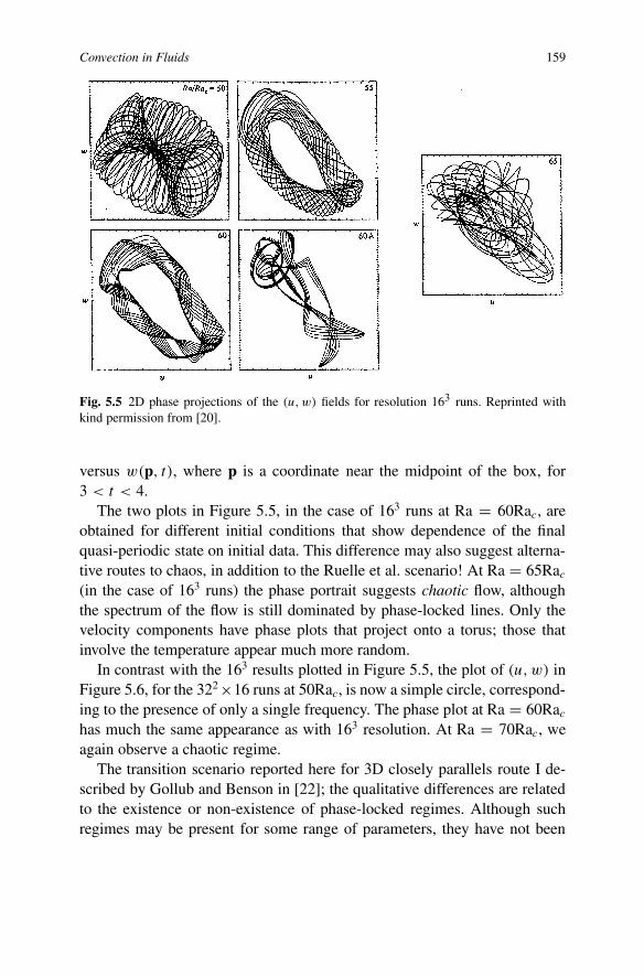
Convection in Fluids 159
Fig. 5.5 2D phase projections of the (u,w) fields for resolution 163 runs. Reprinted withkind permission from [20].
versus w(p, t), where p is a coordinate near the midpoint of the box, for3 < t < 4.
The two plots in Figure 5.5, in the case of 163 runs at Ra = 60Rac, areobtained for different initial conditions that show dependence of the finalquasi-periodic state on initial data. This difference may also suggest alterna-tive routes to chaos, in addition to the Ruelle et al. scenario! At Ra = 65Rac(in the case of 163 runs) the phase portrait suggests chaotic flow, althoughthe spectrum of the flow is still dominated by phase-locked lines. Only thevelocity components have phase plots that project onto a torus; those thatinvolve the temperature appear much more random.
In contrast with the 163 results plotted in Figure 5.5, the plot of (u,w) inFigure 5.6, for the 322×16 runs at 50Rac, is now a simple circle, correspond-ing to the presence of only a single frequency. The phase plot at Ra = 60Rachas much the same appearance as with 163 resolution. At Ra = 70Rac, weagain observe a chaotic regime.
The transition scenario reported here for 3D closely parallels route I de-scribed by Gollub and Benson in [22]; the qualitative differences are relatedto the existence or non-existence of phase-locked regimes. Although suchregimes may be present for some range of parameters, they have not been

160 The Rayleigh–Bénard Shallow Thermal Convection Problem
Fig. 5.6 2D phase projections of the (u,w) fields for resolution 322 × 16 runs. Reprintedwith kind permission from [20].
observed by the above authors because of the coarseness of the partitionthrough parameter space.
In Howard and Krishnamurti’s paper [23], large-scale flow in (turbulent)convection is considered, and to this end the three Fourier components thatlead to Lorenz’s famous three equations (5.44c), were augmented with threeadditional components, leading to a sixth-order system. Namely:
dA
dt= −Pr aA + Pr bD + cBC, (5.55a)
dB
dt= −Pr B − dAC, (5.55b)
dC
dt= −PreC − Pr f F − gAB, (5.55c)
dD
dt= −hD + Ra αA − αAE −
(α
2
)BF, (5.55d)
dE
dt= −4E +
(α
2
)AD, (5.55e)

Convection in Fluids 161
Fig. 5.7 Temperature field at successive time intervals within one oscillation period; Pr =1.0, α = 1.2 and Ra = 55. Reprinted with kind permission from [23].
dF
dt= −mF − Ra αC +
(α
2
)BD. (5.55f)
In this sixth-order dynamical system (5.55a–f), the scalars a, b, c, d, e,f , g, h and m are scalars depending on wave number α. One example ofthe temperature field at times equally spaced within one period is shown inFigure 5.7 for Pr = 1.0, Ra = 55, and similar orbits were found for Pr = 0.1and Pr = 10, for Ra slightly in excess of the critical Ra for the onset ofoscillatory convection

162 The Rayleigh–Bénard Shallow Thermal Convection Problem
The main results of a study of the bifurcations of this six-amplitudes sys-tem (5.55) are that: after the second bifurcation, steady tilted cells are thestable flow, and after the third bifurcation, stable limit cycles are found for arange of Ra. But within this range of Ra, where stable limit cycles are found,there are narrow sub-ranges of aperiodic flows, and the occurrence of thischaotic behaviour is shown to be related to the existence of heterocline orbitpairs. A hot plume or bubble is seen to form in the lower part of the region,then rise and tilt from lower left to upper right. Later, a cold plume forms inthe upper part, sinks and tilts from upper right to lower left. It also shows aleftward-propagating wave in the isotherms near the bottom of the layer anda rightward-propagating wave near the top of the layer.
Concerning the scenarios/routes to chaos, we mention here that usuallythe investigations are linked with three prominent routes which have beentheoretically and experimentally successful:
• first, the Ruelle–Takens–Newhouse scenario in which, after a few bifur-cations, an invariant point set in phase space appears; this set is not atorus but a strange attractor, the motion being aperiodic;
• second, the Feigenbaum scenario in which case the route to chaos in-volves successive periodic doubling (subharmonic) bifurcations of a(simple) periodic flow, the chaotic attractor being not (strictly) a strangeattractor (à la Ruelle–Takens); and
• third, the Pomeau–Manneville scenario, when transition to ‘turbulence’is realized through intermittency.
In Chapter 7 we will return to these three routes to chaos in the case of theBénard deep thermal convection problem. In [19, chapter 10, pp. 387–448]the reader can find an overview relative to a ‘finite-dimensional dynamicalsystem approach to turbulence’ which contains mostly arguments about cur-rent research but is mainly discursive from a fluid dynamicist’s point of view.
5.6 Some Complements
In the vicinity of the threshold of RB thermal convection, it is commonlyknown that the dynamics can be described by means of an amplitude equa-tion; see, for example, the evolution equations (5.35) and (5.43), derivedabove in Section 5.4.
In the 2D case when the starting RB equations are (5.45b) and (5.45c),with boundary conditions (5.47a), and we investigate the nonlinear stability

Convection in Fluids 163
2D, (x, z), problem of an ideal pattern of straight rolls parallel to the y direc-tion, we can derive a so-called ‘Landau–Ginzburg equation’ which has thefollowing reduced form (see e.g., [24]):
∂A
∂t= ∂2A
∂x2+ rA− |A|2A. (5.56)
Usually, a multiple-scales perturbation method is used to compute the coef-ficients in the non-reduced amplitude equation obtained at κ3 order via theFredholm alternative. In derivation of (5.56) the same arguments as in [25]have been used. There is a lot of literature devoted to the analysis of (5.56);for instance, stability analysis of this equation was accomplished in [26] andthe question of existence of a maximal attractor for this equation and itscharacterization was dealt with in [27]. The Landau–Ginzburg equation wasalso analysed numerically in [28]. All these known results for the Landau–Ginzburg equation apply as such to equation (5.56), sometimes with onlyslight modifications, such as a change of variables, are necessary.
The RB problem in rarefied gases has in recent years attracted consider-able interest as a model problem for studying such fundamental issues asthe mechanisms of instability and self-organization at the molecular leveland their relation to macrocospic phenomena (according to [29], where thereader can find various recent references).
In [29] the transition to convection in the RB problem at small Knud-sen (Kn) number is studied via a linear temporal stability analysis of thecompressible ‘slip-flow’ problem. Indeed, significant convection only occursat small O(10−2) Knudsen numbers. In a Cartesian system of coordinates(x1, x2, x3) whose origin lies on the lower wall, x2 = 0, and whose x2 axis ispointing upwards – opposite to the direction of g, the acceleration of gravity– the following dimensionless equations are used as starting equations:
∂ρ
∂t+ ∂
∂xi(ρui) = 0, (5.57a)
ρDui
Dt= −(1/2)
∂p
∂xi+ Kn
∂
∂xj
[2µ
(eij − (1/3)
∂ui
∂xi
)]−
(1
Fr
)ρδi2 ,
(5.57b)
ρDT
Dt=
( γPr
)Kn
∂
∂xj
[κ∂T
∂xj
]− (γ − 1)p
(∂ui
∂xi
)+ 2(γ − 1)Kn�,
(5.57c)p = ρT . (5.57d)
Appearing in (5.57b) and (5.57c) are the rate-of-strain tensor,
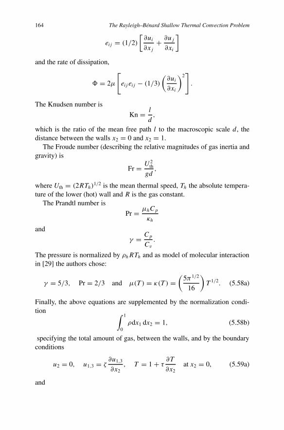
164 The Rayleigh–Bénard Shallow Thermal Convection Problem
eij = (1/2)
[∂ui
∂xj+ ∂uj
∂xi
]
and the rate of dissipation,
� = 2µ
[eij eij − (1/3)
(∂ui
∂xi
)2].
The Knudsen number is
Kn = l
d,
which is the ratio of the mean free path l to the macroscopic scale d, thedistance between the walls x2 = 0 and x2 = 1.
The Froude number (describing the relative magnitudes of gas inertia andgravity) is
Fr = U 2th
gd,
where Uth = (2RTh)1/2 is the mean thermal speed, Th the absolute tempera-ture of the lower (hot) wall and R is the gas constant.
The Prandtl number is
Pr = µhCp
κh
and
γ = Cp
Cv
.
The pressure is normalized by ρhRTh and as model of molecular interactionin [29] the authors chose:
γ = 5/3, Pr = 2/3 and µ(T ) = κ(T ) =(
5π1/2
16
)T 1/2. (5.58a)
Finally, the above equations are supplemented by the normalization condi-tion ∫ 1
0ρdx1 dx2 = 1, (5.58b)
specifying the total amount of gas, between the walls, and by the boundaryconditions
u2 = 0, u1,3 = ζ∂u1,3
∂x2, T = 1 + τ
∂T
∂x2at x2 = 0, (5.59a)
and

Convection in Fluids 165
u2 = 0, u1,3 = −ζ ∂u1,3
∂x2, T = RT − τ
∂T
∂x2at x2 = 1, (5.59b)
respectively.In (5.59a, b), RT = Tc/Th denotes the ratio of cold-and hot-wall tem-
peratures, ζ = 1.1466 Kn and τ = 2.1904 Kn, according to Cercignani’sclassical book [30], where the reader can find for the above problem, thesteady ‘pure convection’
us = 0
the following solution:
Ts = (Ax2 + B)2/3, ρs =(C
Ts
)exp
[−
(6
AFr
)T 1/2s
], (5.60)
in which the constants A, B and C are determined by use of (5.58)–(5.59b).In [29] each of the above-mentioned fields is generically represented by
the sum: steady reference state (5.60) plus perturbed part, and neglectingnonlinear terms a perturbation (linear) problem is derived. From my pointof view, before any numerical simulation, it would be interesting to derive,instead of the above problem, a rational approximate model problem? As afirst (simple) example it seems possible to consider the limiting case when,Kn → 0 and investigate the ‘passage’ to a continuum regime!
If we observe that Kn = M/Re, then Kn � 1 is realized if
(1) the Mach number M � 1 (hyposonic regime [32], but see also [33])and Re fixed to not very low (Stokes and Oseen case); or,
(2) The Reynolds number Re � 1 (Prandtl boundary layer approximation)with M fixed to not very large (hypersonic case).
However, it seems that this ‘passage’ to a continuum regime is not uniformlyvalid and may locally fail at certain parts of the flow field (see [34, 35]).In [30], the reader can find a very pertinent modern presentation of RarefiedGas Dynamics by Cercignani, and in [31] the 2D problem relative to RB flowof a rarefied gas has been studied by means of a direct numerical simulationmethod. Finally, we note that in Chapter 9, devoted to ‘Atmospheric ThermalConvection Problems’, the reader can find a detailed asymptotic (when M �1) derivation of the Boussinesq approximate equations for a thermally perfectgas – this derivation for a gas being rather different from the derivation, givenin Section 3.3, for a weakly expansible liquid.
Below for the standard RB model problem written in the following form(see, for instance, [36, pp. 51–55]):

166 The Rayleigh–Bénard Shallow Thermal Convection Problem
∂u∂t
+ (u · ∇)u = −∇p +�u + Ra θk,
∇ · u = 0,
Pr
[∂θ
d∂t+ u · ∇θ
]= Raw +�θ, (5.61a)
withu = θ = 0, at z = 0 and z = 1, (5.61b)
we shall now show by energy stability theory that sub-critical instability isnot possible (as has been already noted in Section 3.4).
For this, as in [36], we consider the simplest, natural ‘energy’, for the RBsystem of three equations (5.61a), formed by adding the kinetic and thermalenergies of the perturbations, and so we define:
E(t) = (1/2)‖u‖2 + (1/2)Pr ‖θ‖2, (5.62)
where
‖f ‖2 =∫V
f 2 dV.
We differentiate E(t), substitute for ∂u/∂t and ∂θ/∂t from (5.61a), and usethe boundary conditions, (5.61b), to find
dE
dt= 2 Ra〈wθ〉 − [D(u)+D(θ)], (5.63a)
where D(f ) denotes the Dirichlet integral, e.g.,
D(f ) = ‖∇f ‖2 =∫V
|∇f |2 dV,
and
〈fg〉 =∫V
fg dV.
Then we introduce
I = 2〈w〉 and D = D(u)+ D(θ),
such that, from (5.63a), we can write:
dE
dt= Ra I −D ≤ RaD
[(1
Ra
)−
(1
RE
)], (5.63b)
where RE is defined by

Convection in Fluids 167
1
RE
= maxH
(I
D
), with H the space of admissible solutions.
If now Ra < RE, then
Ra
[(1
Ra
)−
(1
RE
)]=
[(RE − Ra)
RE
]= a > 0,
and from (5.63b),dE
dt≤ −aD ≤ −2aλ1E, (5.63c)
where we have also used the classical Poincaré’s inequality; from this in-equality
λ1‖u‖2 ≤ ‖∇u‖2, λ1 > 0.
Finally, by integration,
E(t) ≤ E(0) exp[−2aλ1t], (5.63d)
from which we see that
E → 0 at least exponentially fast as t → ∞. (5.64)
This demonstrates that, provided Ra < RE is satisfied, the conduction mo-tionless solution us = 0 and T = Ts(z) = Tz=0 − βsz, is nonlinearly stablefor all initial disturbances.
One the other hand, the Euler–Lagrange equations for the maximum, inthe above definition, of RE are found by using the calculus of variations andgives
�u + REθk = −∇p; ∇ · u = 0; �θ + REw = 0,
together with the same boundary conditions as (5.61b) and the ‘periodicity’conditions.
In such a case RE satisfies the eigenvalue problem for the classical linearproblem, but with σ = 0 (see (3.30a) with (3.30c–e)). Thus, for the standardRB problem
RE ≡ RaL – the lowest eigenvalue of the linearized theory.
Furthermore, we have the confirmation that [36]:
the linear instability boundary ≡ the nonlinear stability boundary, and sono sub-critical instabilities are possible.

168 The Rayleigh–Bénard Shallow Thermal Convection Problem
In [37] the reader can find various aspects of theoretical analysis of the sta-bility of convective motions.
It is now very well established, theoretically and experimentally, that inthe classical Bénard simple problem for a weakly expansible liquid layer,heated from below, separated from ambient air by an upper, deformablefree surface, buoyancy (a volume-temperature-dependent density effect) ismore important for a relatively thick layer, while the thermocapillarity(an interfacial/thermocapillary-temperature-dependent free surface tension-Marangoni effect) plays the dominant role in the case of significantly thinlayers (or under microgravity conditions).
However, the case where both effects should be taken into account is themost typical in various (other than the classical Bénard convection problem)convection problems. Here, concerning this question, we mention the papersby Braunsfurth and Homsy [38], and Boeck et al. [39] and the reader canfind various other references in both these papers. For instance, the convec-tive phenomena in the presence of an interface in a two-layer system haveattracted great attention specifically due to numerous technological applica-tions (see, for example [39, 40]).
Usually, when the temperature grows, the interfacial tension can decrease(the normal Marangoni effect), but in some cases – for special liquids, see,e.g., [41] and references therein – the interfacial tension increase (the anom-alous Marangoni effect). As this is well explained in [38], in a one-layersystem (heated from below, as in Bénard experiments), the buoyancy vol-ume forces and thermocapillary interfacial stresses act in the same directionand produce together a stationary instability, provided the Marangoni effect(for a thin layer) is normal.
For two-layer systems with an interface, the situation is more intricateand requires obviously a carefully rational analysis to obtain an approximatetheoretical model with possibly both, Rayleigh and Marangoni, effects. In-deed, if the flow in the lower layer is dominant, the actions of buoyancy andthermocapillary effect are similar to those in the one-layer system (in [38]the liquids are situated between rigid horizontal plates that are kept at differ-ent temperatures). If the flow in the upper layer is dominant, the buoyancyforces and thermocapillary stresses act in oposite directions – their compe-titions lead to a stabilization of the stationary instability, as well as to thegeneration of a specific kind of linear oscillatory instability, which has beenpredicted theoretically [42] and observed in experiments [43]. In the caseof the anomalous thermocapillary effect, one can obtain an oscillatory insta-bility when the flow in the lower layer is dominant, and only a stationaryinstability in the opposite case [44].

Convection in Fluids 169
Fig. 5.8 Schematic view of the geometry of the problem considered in [38]. Reprinted withkind permission from [38].
In fact, combined thermocapillary-buoyancy convection occurs in a va-riety of different applications. In cavity (see Figure 5.8) this problem hasbeen investigated in [38], where the reader can find various references re-lated mainly to various experimental studies. A dimensionless analysis fora rectangular container is described by two aspects ratios: Ax = d/h andAy = w/h.
The strength of the buoyancy forces is represented by Ra, and the strengthof the surface tension driving forces is given by Ma.
The dynamic Bond number G is often used as a measure of the relativestrength of buoyancy to thermocapillarity driving forces; the capillary num-ber, Ca, gives an indication of the possible surface deformation due to thesurface forces. Obviously, a rational modelling of the above problem is aninteresting, but certainly difficult, task!
References
1. P.G. Drazin and W.H. Reid, Hydrodynamic Stability. Cambridge University Press, Cam-bridge, 1981.
2. C. Ruyer-Quil, B. Scheid, S. Kalliadasis, M.G. Velarde and R.Kh. Zeytounian, Thermo-capillary long-waves in a liquid film flow; Part 1: Low-dimensional formulation. J. FluidMech. 538, 199–222, 2005.
3. B. Scheid, C. Ruyer-Quil, S. Kalliadasis, M.G. Velarde and R.Kh. Zeytounian, Thermo-capillary long-waves in a liquid film flow; Part 2: Linear stability and nonlinear waves.J. Fluid Mech. 538, 223–244, 2005.
4. E.M. Sparrow, R.J. Goldstein and V.K. Jonsson, Thermal instability in a horizontal fluidlayer: Effect of boundary conditions and non-linear temperature profile. J. Fluid Mech.18, 513–528, 1964.

170 The Rayleigh–Bénard Shallow Thermal Convection Problem
5. S. Chandrasekhar, Hydrodynamic and Hydromagnetic Stability. Clarendon Press, Ox-ford, 1961. See also Dover Publications, New York, 1981.
6. J.S. Turner, Buoyancy Effects in Fluids. Cambridge, Cambridge University Press, 1973.7. M.G. Velarde and C. Normand, Sci. Amer. 243(1), 92, 1980.8. C. Normand, Y. Pomeau and M.G. Velarde, Convective instability: A physicist’s ap-
proach. Rev. Mod. Phys. 49(3), 581–624, 1977.9. A.V. Getling, Rayleigh Bénard Convection: Structure and Dynamics. World Scientific,
Singapore, 1998.10. E. Bodenschatz, W. Pesch and G. Ahlers, Recent developments in Rayleigh–Bénard con-
vection. Annu. Rev. Fluid Mech. 32, 709–778, 2000.11. P.C. Dauby and G. Lebon, Bénard–Marangoni instability in rigid rectangular containers.
J. Fluid Mech. 329, 25–64, 1996.12. R.Kh. Zeytounian, Mécanique des Fluides Fondamentale. Springer-Verlag, Heidelberg
1991.13. A.C. Newell and J. Whitehead, Finite bandwidth, finite amplitude convection. J. Fluid
Mech. 38(2), 279–303, 1966.14. P. Coullet and P. Huerre, Resonance and phase solitons in spatially-forced thermal con-
vection. Physica D 23, 27–44, 1986.15. L.D. Landau, On the problem of turbulence. C.R. Acad. Sci. URSS 44, 311–314, 1944.
See also Collected Papers, 387–391, Oxford, 1965.16. E.N. Lorenz, Deterministic nonperiodic flow. J. Atmospheric Sci. 20, 130–141, 1963.17. C. Sparrow, The Lorenz Equations: Bifurcations, Chaos and Strange Attractors.
Springer, 1982.18. J.K. Platten and J.C. Legros, Convection in Liqids. Springer-Verlag, New York, 1984.19. R.Kh. Zeytounian, Theory and Applications of Viscous Fluid Flows. Springer-Verlag,
Heidelberg, 2004.20. J.H. Curry et al., Order and disorder in two- and three-dimensional Bénard convection.
J. Fluid Mech. 147, 1–38, 1984.21. S. Orszag, Studies Appl. Math. L4, 293–327, 1971.22. J.P. Gollub and S.V. Benson, Many routes to turbulent convection. J. Fluid Mech. 100,
449–470, 1980.23. L.N. Howard and R. Krishnamurti, Large-scale flow in turbulent convection: A mathe-
matical model. J. Fluid Mech. 170, 385–410, 1986.24. Z. Charki and R.Kh. Zeytounian, The Bénard problem for deep convection: Derivation
of the Landau–Ginzburg equation. Int. J. Engng. Sci. 33(12), 1839–1847, 1995.25. D. Siggia and A. Zippelius, Stability of finite-amplitude convection. Phys. Fluids 26,
2905, 1983.26. P. Coullet and S. Fauve, Propagative phase dynamics for systems with Galilean invari-
ance. Phys. Rev. Lett. 55, 2857–2859, 1985.27. C. Doering, J. Gibbon, D. Holm and B. Nicolaenko, Low-dimensional behaviour in the
complex Ginzburg–Landau equation. Nonlinearity 1, 279–309, 1988.28. L.R. Keefe, Dynamics of perturbed wavetrain solutions to the Ginzberg–Landau equa-
tion. Stud. Appl. Math. 73, 91, 1985.29. A. Manela and I. Frankel, On the Rayleigh–Bénard problem in the continuum limit:
Effects of temperature differences and model of interaction. Phys. Fluids 17, O36101-1–O36107, 2005.
30. C. Cercignani, Rarefied Gas Dynamics. Cambridge, Cambridge University Press, 2000.31. S. Stefanov, V. Roussinov and C. Cercignani, Rayleigh–Bénard flow of a rarefied gas and
its attractors. I. Convection regime. Phys. Fluids 14, 2255, 2002.

Convection in Fluids 171
32. R.Kh. Zeytounian, Topics in Hyposonic Flow Theory. Lecture Notes in Physics, Vol. 672.Springer-Verlag, Berlin/Heidelberg, 2006.
33. J. Frölich, P. Laure and R. Peyret, Phys. Fluids A 4, 1355, 1992.34. G. Bird, Molecular Gas Dynamics and the Direct Simulation of Gas Flows. Clarendon,
Oxford, 1994.35. I. Boyd, In: Rarefied Gas Dynamics, A.D. Ketsdever and E.P. Muntz (Eds.), American
Institute of Physics, New York, p. 899, 2003.36. B. Straughan, The Energy Method, Stability, and Nonlinear Convection. Springer-Verlag,
New York, 1992.37. D.D. Joseph. Stability of Fluid Motions II. Springer-Verlag, Berlin, 1976.38. M.G. Braunsfurth and G.M. Homsy, Combined thermocapillary-buoyancy convection in
a cavity. Part II. An experimental study. Phys. Fluids 9(5), 1277–1287, 1997.39. T. Boeck, A. Nepomnyashchy, I. Simanovskii, A. Golovin, L. Braverman and A. Thess,
Phys. Fluids 14(11), 3899–3911, 2002.40. L. Ratke, H. Walter and B. Feuerbacher (Eds.), Materials and Fluids under Low Gravity.
Springer-Verlag, Berlin, 1996.41. H.C. Kuhlmann, Thermocapillary Convection in Models of Crystal Growth. Springer-
Verlag, Berlin, 1999.42. J.C. Legros, Acta Astron. 13, 697, 1986.43. I.B. Simanovskii and A.A. Nepomnyaschy. Convective Instabilities in Systems with In-
terface. Gordon and Breach, 1993.44. A. Juel et al., Surface tension-driven convection patterns in two liquid layers. Physica D
143, 169–186, 2000.45. L.M. Bravermam et al., Convection in two-layer systems with an anomalous thermocap-
illary effect. Phys. Rev. E 62, 3619–3631, 2000.

Chapter 6The Deep Thermal Convection Problem
6.1 Introduction
As written in Straughan’s book [1] (first published in 1993):
an interesting model of thermal convection for a deep layer of fluid isdeveloped by Zeytounian in 1989 [2]. A linear and weakly nonlineartheory for this model is presented by Errafiy and Zeytounian [3], andtransition to chaos results by Errafiy and Zeytounian [4]; sharp nonlin-ear energy stability bounds are derived by Franchi and Straughan [5].
However, in this same direction, at the University of Lille I (Laboratoire deMécanique de Lille, Bâtiment ‘Boussinesq’), Charki published during theyears 1993–1965 three papers relative to: stability [6], existence and unique-ness [7] and the well-posedness of the initial value problem [8]. Finally,we mention the two papers by Charki and Zeytounian [9, 10], where theLorenz system of three equations and the Landau–Ginzburg amplitude equa-tion, both associated to deep convection equations, were derived.
The major interest of ‘deep (Bénard) convection’ (DC) equations (as op-posed to ‘shallow (RB) convection’ equations) is, on the one hand, the pres-ence of the viscous dissipation (non-Boussinesq) term in these equations and,on the other hand, the fact that these DC, à la Zeytounian, convection equa-tions contain a new parameter related to the depth of the layer and called the‘depth parameter’.
Concerning the Hills and Roberts [11] approach, the reader is once moreinvited to re-read Sections 2.7 and 3.6. For the Hills and Roberts model,linear and nonlinear stability results were obtained by Richardson [12].
In this chapter, we assume from the start that the deep fluid layer is limitedby two horizontal rigid plates, z = 0 and z = d, in a Cartesian system of
173

174 The Deep Thermal Convection Problem
coordinates (x, y, z); this seems a limitation, but this limitation is justified,because the main driving, buoyancy force is again governed by the Grashof–Rayleigh number and the thickness of the layer is large.
Indeed, we now see that such an assumption is well founded, becausethe smallness of the Froude number ensures the significant driving role tobuoyancy, via the Grashof number, which is the ratio of the expansibilitysmall parameter ε to the small squared Froude number.
Below, in Section 6.2, as dominant dimensionless equations we choose,for the dimensionless (delete the prime) functions u, π and θ , according to(3.6b, c, d), equations (3.11), (3.14) and (3.15). The boundary conditions atz = 0 and z = 1 are (3.20a, b).
6.2 The Deep Bénard Thermal Convection Problem
The deep dissipative convective layer case is strongly related to (see (4.27c))the conditions
Fr2 � 1, ε � 1 and Bo � 1, (6.1a)
withεBo = O(1), (6.1b)
and alsoε
Fr2 = Gr = O(1). (6.1c)
With relations (6.1a–c), when ε and Fr2 both tend to zero and Bo tends toinfinity, we derive (ε being the main small parameter, when we take intoaccount (6.1b) and (6.1c)) from dominant dimensionless equations (3.11),(3.14) and (3.15), for the leading functions
limε→0
(u, π, θ) = (uD, πD, θD), (6.2)
the following system of deep convection (DC) equations:
∇uD = 0, (6.3a)
duDdt
+ ∇πD − Gr θDk = �uD, (6.3b)
{1 −Di[(pd)′ + 1 − z]}dθDdt
=(
1
Pr
)�θD + (1/2 Gr)Di
[∂uDi
∂xj+ ∂uDj
∂xi
]2
.
(6.3c)

Convection in Fluids 175
where
Di = gαdd
Cd
(6.4)
is our ‘depth’ parameter defined by δ in [2]. For the DC equations (6.3a–c)we write as boundary conditions:
uD = 0 and �D = 1 on z = 0; uD = 0 and �D = 0 on z = 1. (6.5)
In [2], in equation (6.3c) the term (pd)′ is absent because we have neglected
pd in (3.6c) which defines π . As in [2], it is judicious to introduce, insteadof θD , a temperature perturbation
� =(
1
Pr
)Gr [�D + z− 1]
and instead of πD, a pressure perturbation
� =(
1
Pr
) {πD + Gr z
[( z2
)− 1
]}.
If we change also uD to (1/Pr)v and t to τ and omit the term (pd)′ in (6.3c),
then we find again our DC system of equations (4.6) from [2]. Namely:
∇ · v = 0, (6.6a)(
1
Pr
)dvdτ
+ ∇�−�k = �v, (6.6b)
[1 +Di(1 − z)][
d�
dτ− Ra (v · k)
]= ��+ 2Di[D(v) : D(v)], (6.6c)
v = 0 and � = 0 at z = 0 and z = 1, (6.6d)
whereD(v) = (1/2)[∇v + (∇v)T ] (6.6e)
is the rate of deformation tensor.If we now consider the 2D case (which is judicious at the onset of deep
convection) where parallel convective rolls originate, the velocity vector fieldv, becomes perpendicular to the rolls axis and the 3D equations (6.6a–c) areinvariant under the action of translation along the rolls axis.
In such a case, in time-space (τ , x1 = x, x3 = z), for u and w componentsof a 2D velocity vector, we write
u = ∂ψ
∂zand w = −∂ψ
∂x, (6.7)

176 The Deep Thermal Convection Problem
since, instead of (6.6a), we have in the 2D case
∂u
∂x+ ∂w
∂z= 0.
In (6.7), ψ(t, x, z) is the stream function and with �(t, x, z), both are so-lutions of the following system of two equations (after the elimination of�):
(1
Pr
) [∂
∂t+
(∂ψ
∂z
)∂
∂x−
(∂ψ
∂x
)∂
∂z
]�2ψ + ∂�
∂x= �2(�2ψ); (6.8a)
χ(z)
[∂
∂t+
(∂ψ
∂z
)∂
∂x−
(∂ψ
∂x
)∂
∂z
]� + Ra
(∂ψ
∂x
)
= �2� + δ
[4
(∂2ψ
∂x∂z
)2
+(
∂2ψ
∂z2− ∂2ψ
∂x2
)2]
, (6.8b)
with �2 = ∂2/∂z2 + ∂2/∂x2 and χ(z) = 1 + δ(1 − z), Di ≡ δ ∈ [0, 1].For these DC equations (6.8a, b) we write as boundary conditions:
ψ = 0,∂ψ
∂z= 0, or
∂2ψ
∂z2= 0, and � = 0 at z = 0 and z = 1
(6.8c)according to the nature of the boundary.
We observe that the Lorenz system in [9], and the amplitude Landau–Ginzburg equation in [10], have been derived for the 2D system (6.8a, b)with the conditions ψ = 0, ∂2ψ/∂z2 = 0, and � = 0 at z = 0 and z = 1.
Obviously when Di ≡ δ → 0, one obtains, instead of (6.6a–c) and (6.8a,b), the corresponding 3D and 2D classical RB system of shallow convectionequations.
6.3 Linear – Deep – Thermal Convection Theory
The linear theory, when the deep convection equations (6.6a–c) are lin-earized, relative to the zero solution (v = 0, � = 0, � = 0), for smallperturbations (v′, �′, �′) – ignoring the nonlinear terms – gives the follow-ing system of three equations:
∇ · v′ = 0, (6.9a)

Convection in Fluids 177(1
Pr
)∂v′
∂τ+ ∇�′ −�′k = �v′, (6.9b)
[1 + Di(1 − z)][∂�′
∂τ− Ra (v′ · k)
]= ��′. (6.9c)
The linear system (6.9a–c) was investigated carefully by Errafiy [13] in the2D case when v′ = (u′, w′) in time space (τ, x, z). In this case, with thestream function ψ ′(τ, x, z) such that
u′ =(
1
Pr
)∂ψ ′
∂z, w′ = −
(1
Pr
)∂ ′
∂x,
after the elimination of the pressure �′, we get for ψ ′(τ, x, z) and �′(τ, x, z)the following system of two linear equations (µ = δ/[1 + (δ/2)]):
Pr∂ψ ′
∂τ+ ∂�′
∂x= Pr�2(�2ψ
′); (6.10a)
Prλ(z)
[∂�′
∂τ+ Ra
∂ψ ′
∂z
]=
[1 −
(µ2
)]�2�
′, (6.10b)
whereλ(z) = 1 + µ[(1/2) − z] and
µ
δ=
[1 −
(µ2
)].
In the free-free case, the boundary conditions are
ψ ′ = ∂2ψ ′
∂z2= �′ = 0, at z = 0, 1, (6.11a)
∂�′
∂x= ψ ′ = ∂2ψ ′
∂x2= 0, at x = 0 and x = l0, (6.11b)
where l0 is the horizontal dimensionless length of a DC cell.A Galerkin formulation, with as representation
ψ ′ = �An(t) sin(nπz) sin(q0x), (6.12a)
�′ = �Bn(t) sin(nπz) sin(q0x), (6.12b)
where n = 1 to N , and q0 = π/l0 – after a quite lengthy but straightforwardcalculation (analogous to derivation of the Lorenz system of three equationsin Section 5.5 – gives a system of 2N ordinary differential equations whichcan be represented via the matrix Df
f as
dFdτ
= Df
f F, where F = (X1, X2, . . . , XN ;Y1, Y2, . . . , YN), (6.13)

178 The Deep Thermal Convection Problem
Fig. 6.1 Matrix of Dff for the system of 2N ODE. Reprinted with kind permission from [13].
and the general structure of this matrix Df
f in (6.12), is represented in Fig-
ure 6.1. In this figure, the coefficients Dij = Di
j of the matrix Df
f for N = 3are given in [3, p. 628].
For further details, see the paper by Errafiy and Zeytounian [3] andErrafiy’s doctoral thesis [13]. We see that, if the matrix Df
f is real and sym-metric then can have only real eigenvalues. In this case oscillatory instabilityis impossible, and this is a classical proof of the principle of exchange ofstabilities for our linear DC problem (6.10a, b), with (6.11a, b) when δ �= 0.As a consequence, the principle of exchange of stabilities being proved forthe above linear DC free-free problem (6.10a, b) and (6.11a, b), it is possibleto consider only the stationary linear problem to seek the marginal states andthe critical value of the Rayleigh number.
In the rigid-free case (the case of ‘oceanic circulation’) the boundary con-ditions are
ψ ′ = ∂ψ ′
∂z= �′ = 0, at z = 0, (6.14a)
ψ ′ = ∂2ψ ′
∂z2= �′ = 0, at z = 1. (6.14b)

Convection in Fluids 179
In this case, using again the Galerkin technique, but with a modified repre-sentation for ψ ′, instead of (6.12a) we write
ψ ′ = �An(t)ψn(z) sin(q0x), n ≥ 1, (6.15a)
where for ψn(z) we have an explicit formula (see [3, (2.13), with (2.14)]. Wecan write, again, the resulting system of ordinary differential equations in theform (6.13). In the particular case when n = 1 (one component representa-tion for ψ ′ and �′), we easily show that the corresponding matrix is real andsymmetric and can have only two real eigenvalues. In this case, at the steadylinear state, we have that the neutral stability curve is given by the followingequation:
Ra − αµRa − β(µδ
)= 0, (6.16)
where the coefficients α and β are functions of four scalars which appear inthe formula for the function ψn(z), in representation (6.15a) of ψ ′.
When n = 2 (two-components solution) the matrix is symmetric but notreal. In this case oscillatory instability is possible and it is necessary to com-pare the critical Rayleigh number for stationary instability Rast
c with that foroscillatory instability Raosc
c . For this we can take into account the classicalRouth–Hurwitz criterion and Orlando’s formula (see [14, pp. 231–234]). Nu-merical calculation shows that, for all δ,
Rastc < Raosc
c (6.17)
and the validity of the principle of exchange of stabilities is clearly evident,independently of the value of the depth parameter. According to the above re-sult we can consider a stationary DC linear problem, which is written belowfor ψ ′ and the function
T =(
1
Pr
)∂�′
∂x.
Namely�2(�2ψ
′) = T , (6.18a)
�2T = Ra[1 + δ(1 − z)]∂2ψ ′
∂z′2 . (6.18b)
By analyzing the disturbance ψ ′ and T into normal modes, we seek solutionsof (6.18a, b) which are of the form
ψ ′ = W(z)f (x) and T = �(z)f (x), (6.19a)
with

180 The Deep Thermal Convection Problem
d2f
dx2+ q2
0f = 0, q20 = const. (6.19b)
In particular, for the rigid-free case (which is the more difficult case) weobtain the following problem for W(z) and �(z):
(d2
dz2− q2
0
)W = �, (6.20a)
(d2
dz2− q2
0
)� = −Ra q2
0 [1 + δ(1 − z)]W, (6.20b)
with
0 = W = dW
dz= 0 at z = 0,
� = W = d2W
dz2= 0 at z = 1.
As in the classic, à la Chandrasekhar [15], approach, we suppose that for �the solution is
� = ��nα2n sin(nπz), n > 1.
Substituting this solution for � in equation (6.20a), we can write the follow-ing solution for W :
W = ��nψn(z), n > 1,
where ψn(z), for the rigid-rigid case, is an explicit function of z which ap-pears also in the representation (6.15a) of ψ ′ using the Galerkin technique.
Now substituting for � and W the above expressions and taking into ac-count the explicit form of ψn(z), we obtain the following condition:
��n
{α3n
Ra q20 [1 + (δ/2)] sin(nπz)− ψn(z)
}= 0, n > 1. (6.21a)
Multiplying (6.21a) by sin(mπz) and integrating over the range of z, weobtain a system of linear homogeneous equations for the constants �n – therequirement that these constants are not all zero leads to the secular equation
det
{α3n
Ra q20 [1 + (δ/2)]δnm + 2Km
n
}= 0, (6.21b)
where 2Kmn is determined in an explicit form (see [3, (3.11)]). With the aid
of (6.21b) and the expression for 2Kmn , Errafiy obtained the critical Rayleigh
numbers for different values of δ for the three cases: free-free, rigid-rigid and

Convection in Fluids 181
rigid-free. We note that the critical Rayleigh numbers, for different values ofδ, decrease when δ increases from the value δ = 0 to δ = 1. As a result:when the depth parameter δ increases, the layer of (weakly) expansible liquidbecomes very much more stable.
In [3], the reader can find also an approximate solution of the steady-stateproblem (6.20a, b) for
µ = 2δ
(2 + δ)� 1,
by a perturbation method.In particular for the rigid-rigid case, for the critical Ra, we obtain the
following approximate formula (with q0 = 3.117):
Ra =[
1707.9
(1 + δ/2)
]{1 − 7.61 × 10⁻³
[δ
(2 + δ)
]}, (6.21c)
and this formula (6.21c) gives good values for Rac even when δ = 1!Finally, in [3], the reader can find also a direct proof of the Principle Ex-
change of Stabilities for the free-free case, deduced from an explicit relationobtained from the linear system of two equations:
Pr
[λ−
(d2
dz2− q2
0
)](d2W
dz2− q2
0W
)= −�, (6.22a)
{Prλ− [(d2/dz2 − q2
0 )][1 + δ(1 − z)]
}� = Pr Ra q2
0W. (6.22b)
Namely, as a direct consequence of (6.22a, b), we derive the following inte-gral relation:
Imag (λ)
{∫ 1
0
[∣∣∣∣d�
dz
∣∣∣∣2
+ q20 Ra Pr
∣∣∣∣d2W
dz2− q2
0W
∣∣∣∣2
dz
]}= 0; (6.23)
the quantity inside the curly brackets being positive definite for Ra > 0, wehave obviously
Imag (λ) = 0, (6.24)
and this establishes that λ is real for Ra > 0 and for all δ > 0, and that theprinciple of the exchange of stabilities is valid for the thermal DC problem inthe free-free case. An interesting observation is linked with the system of twoequations (6.20a, b), for W(z) and �(z), which appears as very similar to theadjoint system for the classical Couette flow (see [15, sections 71, 130]) –this remark possibly leads to a complementary method for investigation ofthe problem (6.20a, b).

182 The Deep Thermal Convection Problem
6.4 Routes to Chaos
In [4], the partial differential equations governing two-dimensional ther-mal DC, with free-free conditions has been reduced, again according to theGalerkin method, to a set of two ordinary nonlinear differential evolution (intime) equations for two amplitudes Apq(t) and Bpq(t). To slightly change thedefinition of Apq(t) and Bpq(t) by the introduction of two new amplitudes,Xpq(t) and Ypq(t), and then replacing the double subscript (pq) by a singlesubscript (n), the coupled equations for (Xpq(t), Ypq(t)) can be written as
dZn
dt= �mamnZm + �m�lQnmlZmZl, (6.25)
m = 1 to N and 1 = m to N , where the amplitude variables(Z1, Z2, . . . , ZN) are respectively the Fourier amplitudes (Xpq(t), Ypq(t)).In [4], for N = 15, all coefficients anm and Qnml have been calculated (asfunctions of Pr, Ra and δ). Errafiy [13] adopts as a truncation scheme:
p + q < K with K = 4.
It is interesting to observe that, if in the classical RB thermal shallow con-vection case (when δ = 0) the amplitudes with (p+q) odd do not contribute– they tend to zero when time tends to infinity even if initially they weredifferent from zero – on the contrary this is not true in the thermal DC case.Indeed, the new (five) odd components which appear in the case when δ �= 0are responsible (‘open the door’) for the appearance ‘in a new space’ of a va-riety of strange attractors via the three main routes to chaos: Ruelle–Takens[16], Feigenbaum [17] and Pomeau–Manneville [18] scenarii.
With N = 15, we have ten equations corresponding to RB convection(only even amplitudes) and five equations connecting with δ �= 0 (odd am-plitudes, as a direct consequence of the non-equivariance of the exact DC 2Dsystem).
We wish to point out two interesting features of our thermal DC model.The first relates to the interactions between the even and odd amplitudes insystem (6.25), even though the depth parameter δ is very small. As a resultwe obtain numerically all three of the routes (scenarios) to chaos, for variousvalues of Pr, δ and
κ = (Ra − Rac)
Rac, (6.26)
The second point relates to the ‘chaotic configuration’ of strange attractorswhen δ is not small, e.g., for δ = 0.6 and δ = 1. When δ is not small the

Convection in Fluids 183
Fig. 6.2 Projection onto the (Y,X) plane of successive torii for Pr = 20 and δ = 0.2.Reprinted with kind permission from [13].
chaos appears more rapidly and the corresponding strange attractor is morecomplex (see for example Figures 6.8 and 6.9 below) and it seems that, viathe depth parameter δ a ‘space effect on the temporal chaos is being takeninto account’. In Figure 6.2 above, the successive attractors (for various val-

184 The Deep Thermal Convection Problem
Fig. 6.3 Strange attractor à la Ruelle–Takens for κ = 154, Pr = 20 and δ = 0.2. Reprintedwith kind permission from [13].
Fig. 6.4 ‘Chaotic Feigenbaum’ attractor for κ = 290 and Pr = 100 and δ = 0.1. Reprintedwith kind permission from [13].
ues of κ between 125 and 150) are the 2D torii T2 and the strange attractor,which is represented in Figure 6.3, results from the ‘destroying’ of the lasttorus for the value of κ , quite near to κ = 154, for which the strange attractor,à la Ruelle–Takens, appears. We see that this strange attractor is rather sim-ilar to the well-known Lorenz attractor (see Figures 5.4a–c, in Section 5.5)and seems to have many of the gross features observed in the Lorenz model.Therefore it is an excellent candidate for a higher dimensional analogue. Fora pertinent discussion concerning bifurcations of periodic solutions onto in-variant torii, see [19].
In Figure 6.4, we have represented the Feigenbaumm ‘chaotic’ attractorfor k = 290, Pr = 100 and δ = 0.1 corresponding to successive period dou-bling of Figure 6.5. In Figure 6.5, we have represented the same projectionsas those in Figure 6.2, for various values of κ between 200 and 250, but for

Convection in Fluids 185
Fig. 6.5 Successive period doubling for Pr = 100 and δ = 0.1. Reprinted with kind permis-sion from [13].

186 The Deep Thermal Convection Problem
Fig. 6.6 Temporal evolutions of X(t) and associated attractor in three time intervals (κ =100, Pr = 100, δ = 1). Reprinted with kind permission from [13].
Pr = 100 and δ = 0.1. In this case, curiously, instead of a series of 2D toriiT2, we have a series of periodic regimes with period doublings and the chaosappears for κ = 270.
Strictly speaking, the Feigenbaum chaotic attractor is not a strange at-tractor (see Schuster’s book [20] for the precise definition of this ‘object’)but it is very representative of the chaos when the power spectrum is con-tinuous. In this case the route to chaos involves successive period doubling(subharmonic) bifurcations of a periodic deep thermal convection. It is alsointeresting to observe that for δ = 1 and Pr = 100 (see Figure 6.6) we havefor κ = 100, a phenomenon of intermittency between two periodic regimeswhen the time increases; in such a case we are confronted with a strong in-fluence of the depth parameter δ = 1.
In Figure 6.7, according to the Pomeau–Manneville scenario, we havenumerical evidence of the intermittency for Pr = 10 and δ = 0.1. For κ =130 the bursts are relatively large but for κ = 120 we have a pure periodicregime. The instability occurs through the intermittent regime and for κ =130 the attractor is chaotic.
The numerical route to obtaining chaos via intermittency is ‘fascinating’and confirms very well the Pomeau–Manneville scenario. For κ = 130 we

Convection in Fluids 187
Fig. 6.7 Numerical evidence of the Pomeau–Manneville scenario. Reprinted with kind per-mission from [13].

188 The Deep Thermal Convection Problem
Fig. 6.8 Strange attractor with δ = 1 (κ = 115 and Pr = 10). Reprinted with kind permissionfrom [13].
Fig. 6.9 Strange attractor with δ = 0.6 (κ = 139 and Pr = 20). Reprinted with kind permis-sion from [13].
have the occurrence of a temporal evolution (linked with X(τ)) which alter-nates randomly between ‘long’ regular (laminar) phases (so-called ‘intermis-sions’) and relatively short irregular bursts. We also observe that the numberof chaotic bursts increases with an ‘external’ parameter, which means thatintermittency offers a continuous route from regular to chaotic convection;for our case the increase is from 122 to 130.
As a first example of a strong influence of the depth parameter δ on theroute to chaos, we have represented in Figure 6.8 a strange attractor (when

Convection in Fluids 189
Pr = 10 and δ = 1), for κ = 115; but for a very close value, κ = 114.66, in-stead of this strange attractor we have a simple limit cycle (periodic regime)and more surprisingly for κ = 114.80 the regime is already chaotic.
A second example of the influence/dependence of the depth parameter δon the appearance of a strange attractor is the strange very chaotic attractorin Figure 6.9.
Indeed, when Pr = 20 but δ = 0.1, only for a high value of κ = 160do we obtain a strange attractor similar to the one represented in Figure 6.3,which is much less chaotic than the one in Figure 6.8! Maybe it is interestingto obtain a numerically strange attractor for larger (than δ = 1?) values ofδ! But in such a case, the probability for appearance of attractors being in anexplosive manner, the value seems very high?
6.5 Rigorous Mathematical Results
After the publication of [2], where the thermal DC equations were first de-rived, and the two papers by Errafyi and Zeytounian [3, 4] concerning thelinear theory and routes to chaos for these DC equations had been published,some authors considered the existence, uniqueness and stability of solutionsfor these DC convection equations for various thermal convection problems.In particular, Franchi and Straughan [5] applied a nonlinear energy stabilityanalysis for these deep convection equations. On the other hand, Charki dur-ing the years 1994–1996, at the University of Lille I published three papersrelative to: stability [6], existence and uniqueness of solutions for the steadyproblem [7], and the initial value problem [8].
Before, in 1992, Richardson [12] used a nonlinear stability analysis ofconvection in a generalized (à la Hills and Roberts [11]) incompressiblefluid, the equations governing such a fluid being a particular ad hoc caseof our DC equations. In [6] by Charki, existence and uniqueness of a local intime strong solution for the unsteady DC problem is proved through use of asemigroup theory. The bifurcation problem (for linear and nonlinear cases) isalso dealt with and the possibility of existence of periodic and quasiperiodicsolutions to the DC problem is analyzed.
We observe that under the same assumptions as in Iooss’ paper [21], allthe results there concerning the existence and stability of periodic solutionsare valid for the DC problem; in particular, ‘for the DC problem, subcriticalperiodic motions are unstable, while supercritical periodic motions are stablein the linearized theory’. Charki [7] deals mainly with the steady DC problem

190 The Deep Thermal Convection Problem
in a bounded domain. Existence and uniqueness of solutions is establishedthere for both the linear and the nonlinear problems, subject either to ho-mogeneous or non-homogeneous boundary conditions. The proof is basedon estimates for the linear problem, followed by a fixed point argument. Afixed point argument is also used by Charki in [8] to prove the existenceand uniqueness of solutions for the unsteady DB convection equations ina bounded domain. Using some methods of Solonnikov [22], Charki firstproves a global existence theorem for the linear deep convection equationsin Lq spaces. Then, using classical estimates for the nonlinear terms, he alsoproves a local existence theorem for the nonlinear DB convection equations.As this is mentioned by Padula (University of Ferrara) it is worthy of noticethat the summability exponent, p, must be greater than 5/2, unlike the caseof thin layers where p is only required to be greater than 5/3; but, obviously,the existence of a ‘thin layer’ is excluded in the DC case!
Concerning the paper by Franchi and Straughan [5], the analysis of theseauthors is completely rigorous and, due to the nonlinearities of the systemof equations governing deep convection, requires a generalized energy the-ory. For this, the authors derive from the equations of Zeytounian [2] thefollowing equation for energy:
dE
dt= RI − D + 2
(δ
R
)〈µ(z)θ dij dji〉, (6.27)
where R = √Ra and, in [5], as temperature θ = R� is used, with δ and �,
defined in [2].In (6.27), E, I and D are
E = (1/2 Pr)‖u‖2 + (1/2)‖θ‖2; I = 2〈θw〉, (6.28a)
D = ‖u‖2 + 〈µ|∇θ |2〉 − δ2〈µ3θ2〉 >, (6.28b)
D being positive-definite and [1/(1 + δ)] ≤ µ(z) ≤ 1.Employing Poincaré’s inequality (where π is the pressure)
π2‖θ‖2 ≤ ‖∇θ‖2 ⇒ D ≥ ‖∇u‖2 + k‖∇θ‖2, (6.29)
where
k =[
1
(1 + δ)
]−
(δ2
π2
)> 0.
The difficulty in proceeding from (6.27) is the nonlinear term involving
〈µ(z)θ dij dji〉?

Convection in Fluids 191
To handle the nonlinear term in (6.27), it is necessary to consider an identityfor ‖∇u‖2 (see [23, 24]). After a quite ‘long manipulation’ using variousinequalities (in particular, from Adams’ book [25], and also [24], ‘Cauchy–Schwarz’ and also again Poincaré) and employing the arithmetic mean, theauthors prove that, provided
EG(0) <1
A, then EG(t) → 0 as t → ∞, (6.30a)
see [23, chapter 2].In [5] Charki introduces a generalized energy
EG(t) = E +(
λ
2 Pr
)‖∇u‖2 (6.30b)
RE is defined by
RE = max
(1
D
)on the space of ‘admissible solutions’.
Finally, provided that
(a) R < RE (6.31a)
and
(b) EG(0) <1
A, (6.31b)
with
A =(
23/2 c
R
) {[R
(λ Pr)1/2
]+
[(2
k
)(δ2
λ
)]1/2
+ δ + 2δ
λ[ak]1/2
},
(6.31c)the authors rigorously established nonlinear stability.
In (6.31c), a value for ‘c’ in the current context is contained in [24] and
a = (RE − R)
RE
> 0,
because it is assumed that R < RE.Of course, the stability so obtained is conditional (on the size of the initial
amplitudes), but, due to the nonlinear nature of the DC equation for θ , this isnot unexpected. The number RE(δ) is the nonlinear stability threshold and,in [5], RE(δ) is found from the following system for W(z) and �(z):
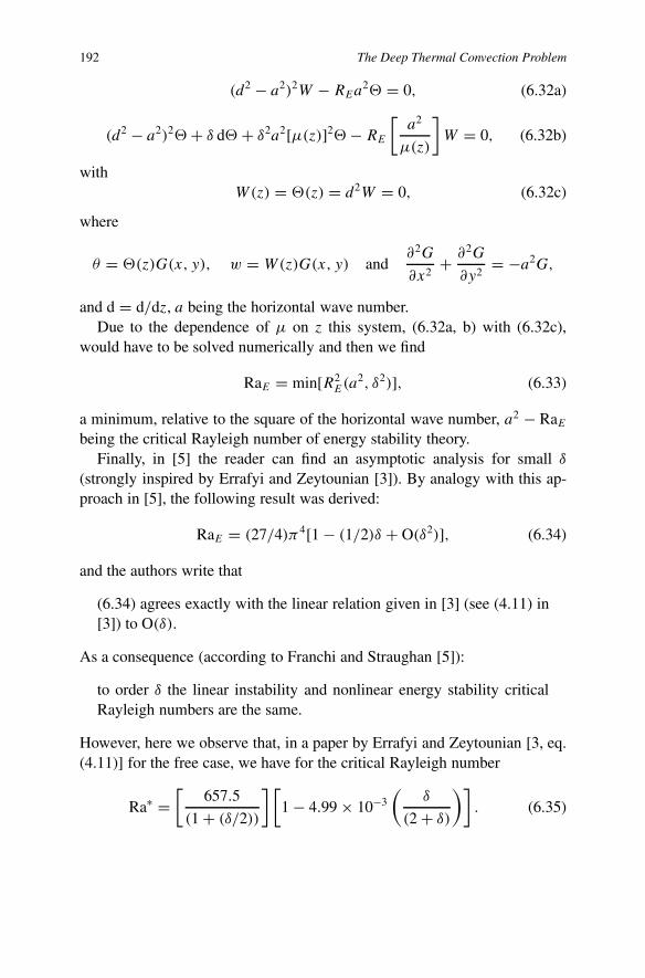
192 The Deep Thermal Convection Problem
(d2 − a2)2W − REa2� = 0, (6.32a)
(d2 − a2)2�+ δ d� + δ2a2[µ(z)]2�− RE
[a2
µ(z)
]W = 0, (6.32b)
withW(z) = �(z) = d2W = 0, (6.32c)
where
θ = �(z)G(x, y), w = W(z)G(x, y) and∂2G
∂x2+ ∂2G
∂y2= −a2G,
and d = d/dz, a being the horizontal wave number.Due to the dependence of µ on z this system, (6.32a, b) with (6.32c),
would have to be solved numerically and then we find
RaE = min[R2E(a
2, δ2)], (6.33)
a minimum, relative to the square of the horizontal wave number, a2 − RaEbeing the critical Rayleigh number of energy stability theory.
Finally, in [5] the reader can find an asymptotic analysis for small δ(strongly inspired by Errafyi and Zeytounian [3]). By analogy with this ap-proach in [5], the following result was derived:
RaE = (27/4)π4[1 − (1/2)δ + O(δ2)], (6.34)
and the authors write that
(6.34) agrees exactly with the linear relation given in [3] (see (4.11) in[3]) to O(δ).
As a consequence (according to Franchi and Straughan [5]):
to order δ the linear instability and nonlinear energy stability criticalRayleigh numbers are the same.
However, here we observe that, in a paper by Errafyi and Zeytounian [3, eq.(4.11)] for the free case, we have for the critical Rayleigh number
Ra∗ =[
657.5
(1 + (δ/2))
][1 − 4.99 × 10⁻³
(δ
(2 + δ)
)]. (6.35)

Convection in Fluids 193
References
1. B. Straughan, Mathematical Aspects of Penetrative Convection. Longman, 1993.2. R.Kh. Zeytounian, Int. J. Engng. Sci. 27(11), 1361–1366, 1989.3. M. Errafyi and R.Kh. Zeytounian, Int. J. Engng. Sci. 29(5), 625, 1991.4. M. Errafyi and R.Kh. Zeytounian, Int. J. Engng. Sci. 29(11), 1363, 1991.5. F. Franchi and B. Straughan, Int. J. Engng. Sci. 30, 739–745, 1992.6. Z. Charki, Stability for the deep Benard problem. J. Math. Sci. Univ. Tokyo 1, 435–459,
1994.7. Z. Charki, ZAMM 75(12), 909–915, 1995.8. Z. Charki, The initial value problem for the deep Benard convection equations with data
in Lq. Math. Models Meth. Appl. Sci. 6(2), 269–277, 1996.9. Z. Charki and R.Kh. Zeytounian, Int. J. Engng. Sci. 32(10), 1561–1566, 1994.
10. Z. Charki and R.Kh. Zeytounian, Int. J. Engng. Sci. 33(12), 1839–1847, 1995.11. R. Hills and P. Roberts, Stab. Appl. Anal. Continuous Media 1, 205–212, 1991.12. L. Richardson, Geophys. Astrophys. Fuid Dynamics 66, 169–182, 1992.13. M. Errafyi, Transition vers le chaos dans le problème de Bénard profond. Thèse de Doc-
torat en Mécanique des Fluides, No. 540, Université des Sciences et Technologies deLille, LML, Villeneuve d’Ascq, 125 pp., 1990.
14. F.R. Gantmacher, Applications of the Theory of Matrices. Interscience, New York, 1959.15. S. Chandrasekhar, Hydrodynamic and Hydromagnetic Stability. Oxford University Press,
1961.16. D. Ruelle and F. Takens, Comm. Math. Phys. 20, 167–192, and 23, 343–344, 1971.17. M.J. Feigenbaum, J. Statist Phys. 19, 25–52, 1978; and Physica D 7, 16–39, 1983.18. Y. Pomeau and P. Manneville, Comm. Math. Phys. 77, 189–197, 1980. See also, P. Man-
neville and Y. Pomeau, Phys. Lett. A 75, 1–2, 1979.19. O.E. Lanford III, Lecture Notes in Mathematics, Vol. 322, Springer-Verlag, Heidelberg,
1973.20. H.G. Schuster, Deterministic Chaos, An Introduction. Physik-Verlag, Weinheim, 1984.21. G. Iooss, Arch. Rat. Mech. Anal. 47, 301–329, 1972.22. V. Solonnikov, J. Soviet Math. 8, 467–529, 1977.23. B. Straughan, The Energy Method, Stability, and Nonlinear Convection, Applied Math-
ematical Sciences, Vol. 91. Springer, Berlin, 1992.24. G.P. Galdi and B. Straughan, Proc. Roy. Soc. London A 402, 257–283, 1995.25. R.A. Adams, Sobolev Spaces. Academic Press, New York, 1975.

Chapter 7The Thermocapillary, Marangoni, ConvectionProblem
7.1 Introduction
It seems very judicious (at least from my point of view) to quote again someremarks about ‘the dynamics of thin liquid films’ from the preface of therecent special issue of Journal of Engineering Mathematics [1]:
A detailed understanding of flows in thin liquid films is important fora wide range of modern engineering processes. This is particularly soin chemical and process engineering, where the liquid films are en-countered in heat-and-mass-tranfer devices (e.g. distillation columnsand spinning-disk reactors), and in coating processes (e.g. spin coat-ing, blade coating, spray painting and rotational moulding). In order todesign these processes for safe and efficient operation it is important tobuild mathematical models that can predict their performance, to haveconfidence in the predictions of the models, and to be able to use themodels to optimize the design and operation of the devices involved.Thin liquid films also occur in a variety of biological contexts. On theother hand, when liquids flow in thin films, the interface (free surface)between the liquid and surrounding (passive!) gas can adopt a rich vari-ety of interesting waveforms – these shapes are determined by a balanceof the principle driving forces, usually including gravity, (temperature-dependent Marangoni phenomena) surface tension and viscous effects.
See, the paper by Trevelyan and Kalliadasis in [1, pp. 177–208]. TheMarangoni effects due to the presence of surfactants are also the subjectof many investigations, see, for instance, the papers by Edmonstone et al. in[1, pp. 141–156] and by Schwartz et al. in [1, pp. 157–175].
195

196 The Thermocapillary, Marangoni, Convection Problem
Over the last 40 years the nonlinear dynamics of a thin liquid film flow-ing down an inclined plane have been extensively studied using the famousBenney equation (see [2] and Section 7.5). In the paper by Oron and Gottliebin [1, pp. 121–140], the problem of the stability threshold predicted by thisBenney equation is revisited. On the other hand:
the lubrication theory and its various extensions is an interesting andchallenging one. Beyond the incorporation of different and more var-ied physical effects, there remain many mathematical challenges in thefield of thin-film flows. The overriding mathematical advantage of thin-film theories is that they take account of a wide separation of scales inthe geometrical configuration under consideration – this affords valu-able simplification, obviating the need for computationally-expensivefully numerical simulations while preserving essential elements of thephysics of the starting system.
Undoubtedly, the 12 papers in [1] are very valuable and very well illustrateboth the wide variety of mathematical methods that have been employed andthe broad range of their application; from this point of view, this specialdouble issue of the Journal of Engineering Mathematics [1] is an ‘recom-mended’ complement to the present chapter. But, once again, various authorsuse ad hoc (non-rational) methods to derive various approximate models andthis, unfortunately, strongly reduces their validity for practical applications!
During recent years, many books have been published in which thermo-capillary, Marangoni convection is discussed. Of particular interest are, first,the book by Colinet et al. [3] which appeared in 2001 and then the bookby Nepomnyashchy et al. [4] that appeared in 2002. In CISM Courses andLectures, No. 428 [5], edited by Velarde and Zeytounian, the readers canfind also various contributions relative to ‘Interfacial Phenomena and theMarangoni effect’ (presented at a Summer Course held at CISM, Udine, inJuly 2000).
Concerning the thermocapillary effect – driving the BM convection – weobserve that, if the (free) surface tension σ changes with temperature T :σ = σ (T ), then
∇‖σ (T ) =[
dσ (T )
dT
]∇‖T ,
where ∇‖ indicates a gradient operator; but the subscript ‘‖’ restricts thecorresponding gradient vector to its surface components. The liquid tends tomove in the direction from lower to higher surface tension (Marangoni effect,see Figure 7.1). The above quantity dσ (T )/dT is negative for practically all

Convection in Fluids 197
Fig. 7.1 BM instability. Reprinted with kind permission from [6].
substances which are relatively easily obtained in an almost pure state (theorder of magnitude is 10−1 to 10−2).
In Figure 7.1, the reader can find a visualization relative to Bénard–Marangoni instability; (a) shows convection cells visible from above in a thinliquid layer and (b) gives a scheme of the convection in BM cells. Thanks tothe Marangoni effect, the free surface (or interface) becomes active in drivingflow or instability in thin liquid layer, films or drops and also bubbles.
We also observe that the ratio between buoyancy (‘Archimedean’ effect)and surface-tension-gradient (Marangoni effect) forces is the dynamic Bondnumber, and when density ρ = ρ(T ), this number is given by
Bd = gd2
[(−dρ(T )/dT )A(−dσ (T )/dT )A
]≡ Gr
Ma. (7.1a)
where, with (7.1b) and (7.2a),
Gr = ε′
Fr2Ad
, (7.1b)

198 The Thermocapillary, Marangoni, Convection Problem
and
Ma =[−dσ (T )
dT
]A
d(Tw − TA
ρ(TA)ν(TA)2, (7.1c)
ε′ =(
1
ρ(TA)
)[−dρ(T )
dT
]A
(Tw − TA), (7.1d)
Fr2Ad = (νA/d)
2
gd, (7.1e)
when as dimensionless temperature we have (see (1.17c)),
� = (T − TA)
(Tw − TA).
For usual values we obtain
Bd ≈ 1, for d ≈ (γσA/gρAαA)1/2 ≈ (1/10) cm
which is the same value for d obtained (see (1.11)) when
Fr2Ad ≈ 1 ⇒ d ≈
(ν2A
g
)1/3
≈ 1.00 mm.
From a physicist’s point of view (see, for instance, [7]) the ratio (7.1a) givesa measure of the relative effectiveness of buoyancy and of surface tensioneffects, each of which results from variation in temperature.
For a given temperature difference, this ratio varies with d2, and as a re-sult surface tension effects dominate for small thickness of the fluid layer, andgravitational ones for very thick layers. Ten years ago, when I first read theabove sentence in [6], I understood that these two effects should be related(certainly) to two particular values of a single dimensionless reference para-meter. A little later on I discovered that, in fact, the Grashof number (7.1b) isa ratio of two dimensionless parameters, ε′ � 1 and Fr2
Ad , and this has beenfor me an indication that the squared Froude number (where the thicknessd of the liquid layer is present) plays this role. This remark allowed me toformulate the following ‘alternative’ [8], published in 1998:
Either the buoyancy is taken into account, and in this case the free-surface deformation effect is negligible and we rediscover the classicalRayleigh–Bénard (RB) shallow convection rigid-free problem or, thefree-surface deformation effect is taken into account and, in a such case,at the leading-order approximation for a weakly expansible fluid, thebuoyancy does not play a significant rôle in the Bénard–Marangoni(BM) thermocapillary instability problem.
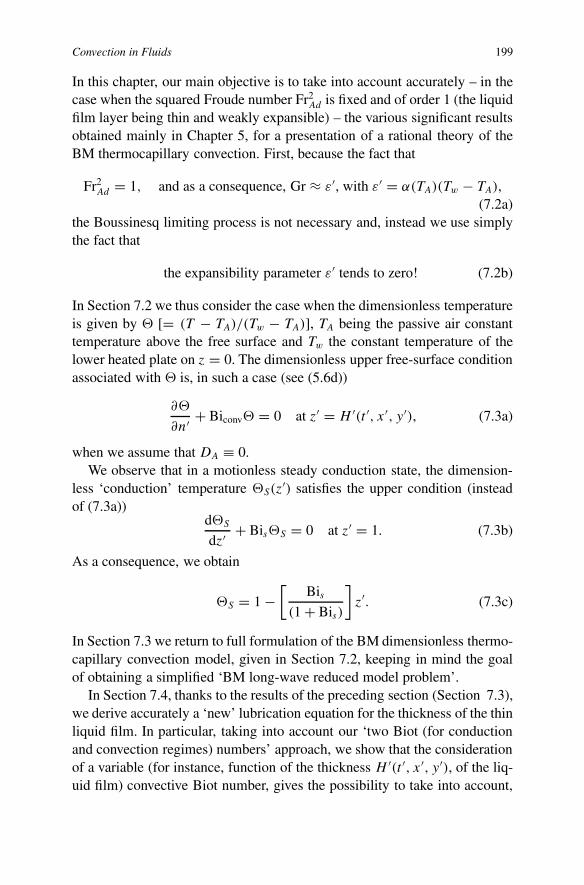
Convection in Fluids 199
In this chapter, our main objective is to take into account accurately – in thecase when the squared Froude number Fr2
Ad is fixed and of order 1 (the liquidfilm layer being thin and weakly expansible) – the various significant resultsobtained mainly in Chapter 5, for a presentation of a rational theory of theBM thermocapillary convection. First, because the fact that
Fr2Ad = 1, and as a consequence, Gr ≈ ε′, with ε′ = α(TA)(Tw − TA),
(7.2a)the Boussinesq limiting process is not necessary and, instead we use simplythe fact that
the expansibility parameter ε′ tends to zero! (7.2b)
In Section 7.2 we thus consider the case when the dimensionless temperatureis given by � [= (T − TA)/(Tw − TA)], TA being the passive air constanttemperature above the free surface and Tw the constant temperature of thelower heated plate on z = 0. The dimensionless upper free-surface conditionassociated with � is, in such a case (see (5.6d))
∂�
∂n′ + Biconv� = 0 at z′ = H ′(t ′, x′, y′), (7.3a)
when we assume that DA ≡ 0.We observe that in a motionless steady conduction state, the dimension-
less ‘conduction’ temperature �S(z′) satisfies the upper condition (instead
of (7.3a))d�S
dz′ + Bis�S = 0 at z′ = 1. (7.3b)
As a consequence, we obtain
�S = 1 −[
Bis(1 + Bis)
]z′. (7.3c)
In Section 7.3 we return to full formulation of the BM dimensionless thermo-capillary convection model, given in Section 7.2, keeping in mind the goalof obtaining a simplified ‘BM long-wave reduced model problem’.
In Section 7.4, thanks to the results of the preceding section (Section 7.3),we derive accurately a ‘new’ lubrication equation for the thickness of the thinliquid film. In particular, taking into account our ‘two Biot (for conductionand convection regimes) numbers’ approach, we show that the considerationof a variable (for instance, function of the thickness H ′(t ′, x′, y′), of the liq-uid film) convective Biot number, gives the possibility to take into account,

200 The Thermocapillary, Marangoni, Convection Problem
in a ‘newly derived’ lubrication equation, the thermocapillary/Marangoni ef-fect, even if the convective Biot number is vanishing (zero)!
Section 7.5 is devoted to an asymptotic detailed derivation of a generalizedà la Benney equation, to the Kuramuto–Sivashinsky (KS) equation, and KS–KdV equation with a dispersive term and also our 1998 IBL non-isothermalsystem of three averaged equations, for thickness (H ), flow rate (q) and (�)related to the temperature across a layer.
In Section 7.6, various aspects of the linear and weakly nonlinear stabilityanalysis of the thermocapillary convection are discussed.
In Section 7.7, devoted to ‘some complementary remarks’, various resultsderived in Sections 7.4 and 7.5 are re-considered and compared with theresults obtained when the dimensionless temperature is given by θ [= (T −Td)/(Tw − Td)], where Td [≡ Ts(z = d)] is the temperature linked withthe steady-state motionless conduction [Ts(z) = Tw − βsd]. The upper free-surface condition associated with θ (see (2.48)) being
∂θ
∂n′ +{
Biconv
Bis(Td)
}[1 + Bis(Td)θ] = 0 at z′ = H ′(t ′, x′, y′) (7.4a)
and the associated θS(z′) satisfy the upper condition (instead of (7.4a), be-
cause in a conduction state Biconv ⇒ Bis(T )d)],dθS
dz′ + 1 + Bis(Td)θS = 0 at z′ = 1, (7.4b)
which leads toθS = 1 − z′. (7.4c)
The above observation shows that it is necessary for each case to be pre-cise and to use the associated steady motionless conduction solution (with asubscript ‘S’) with as Biot number Bis instead of Biconv.
We again stress that the ‘usual, à la Davis’ [41] upper free-surface con-dition for the dimensional temperature θ is obtained from (7.4a) when weidentify (or perhaps confuse) the convection Biot number (variable, Biconv)with the conduction Biot number (constant, Bis(Td)).
7.2 The Formulation of the Full Bénard–MarangoniThermocapillary Problem
Now, our starting dominant, approximate, dimensionless system of threeequations (where the terms proportional to ε′ are taken into account) is given

Convection in Fluids 201
by (5.4a–c) and boundary conditions by (5.5a, b), (5.6a–d). With the abovelimiting process (7.2b), we associate three asymptotic expansions for veloc-ity vector u′, dimensionless pressure
π =(
1
Fr2d
){[(p − pA)
gdρA
]+ z′ − 1
},
and dimensionless temperature �. Namely:
u′ = uBM +ε′u1 +· · · , π = πBM +ε′π1 +· · · , � = �BM +ε′�1 +· · · ,(7.5)
The reader may observe that, only in Chapter 3 (see (3.6c)), for the simpleRayleigh thermal convection problem, we have defined π with (p − pd),and this is justified for a constant thickness liquid layer, d. With (7.2a, b)and (7.5) we obtain as leading-order BM equations (all primes ′ have beendropped, see (5.4a–c)) the following three equations:
∇ · uBM = 0, (7.6a)
duBM
dt+ ∇πBM = �uBM, (7.6b)
Prd�BM
dt= ��BM, (7.6c)
With d/dt = ∂/∂t + uBM · ∇, which are the usual Navier equations (7.6a,b) relative to uBM and πBM, for an incompressible fluid supplemented à laFourier by temperature equation (7.6c) for �BM where Pr is the usual Prandtlnumber at constant temperature TA,
Pr = ν(TA)
κ(TA)with κ(TA) = k(TA)
ρ(TA)Cv(TA),
TA being the temperature of the ambiant passive air above the upper freesurface.
On the other hand, if the boundary conditions for uBM and �BM, at lowerhorizontal plane z = 0, according to (5.5a, b), are simply
uBM|z=0 ≡ (u1BM|z=0, u2BM|z=0, u3BM|z=0) = 0, (7.7a)
and�BM|z=0 = 1, (7.7b)
on the contrary, at the deformable free surface z = H(t, x, y), the upper con-ditions are very complicated. These upper free-surface conditions are derivedfrom (5.6a–d), written with � (see (5.6c–d)).
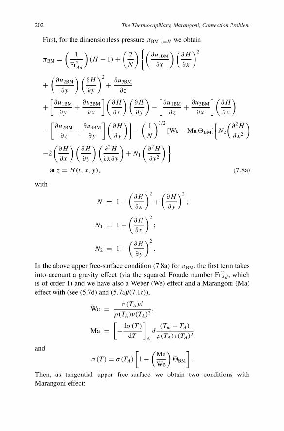
202 The Thermocapillary, Marangoni, Convection Problem
First, for the dimensionless pressure πBM|z=H we obtain
πBM =(
1
Fr2Ad
)(H − 1) +
(2
N
) {(∂u1BM
∂x
)(∂H
∂x
)2
+(
∂u2BM
∂y
) (∂H
∂y
)2
+ ∂u3BM
∂z
+[∂u1BM
∂y+ ∂u2BM
∂x
](∂H
∂x
)(∂H
∂y
)−
[∂u1BM
∂z+ ∂u3BM
∂x
](∂H
∂x
)
−[∂u2BM
∂z+ ∂u3BM
∂y
](∂H
∂y
)}−
(1
N
)3/2
[We − Ma �BM]{N2
(∂2H
∂x2
)
−2
(∂H
∂x
)(∂H
∂y
) (∂2H
∂x∂y
)+ N1
(∂2H
∂y2
)}
at z = H(t, x, y), (7.8a)
with
N = 1 +(
∂H
∂x
)2
+(
∂H
∂y
)2
;
N1 = 1 +(
∂H
∂x
)2
;
N2 = 1 +(
∂H
∂y
)2
.
In the above upper free-surface condition (7.8a) for πBM, the first term takesinto account a gravity effect (via the squared Froude number Fr2
Ad , whichis of order 1) and we have also a Weber (We) effect and a Marangoni (Ma)effect with (see (5.7d) and (5.7a)/(7.1c)),
We = σ (TA)d
ρ(TA)ν(TA)2,
Ma =[−dσ (T )
dT
]A
d(Tw − TA)
ρ(TA)ν(TA)2
and
σ (T ) = σ (TA)
[1 −
(Ma
We
)�BM
].
Then, as tangential upper free-surface we obtain two conditions withMarangoni effect:
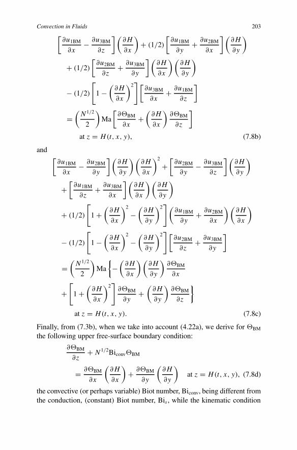
Convection in Fluids 203[∂u1BM
∂x− ∂u3BM
∂z
] (∂H
∂x
)+ (1/2)
[∂u1BM
∂y+ ∂u2BM
∂x
] (∂H
∂y
)
+ (1/2)
[∂u2BM
∂z+ ∂u3BM
∂y
] (∂H
∂x
)(∂H
∂y
)
− (1/2)
[1 −
(∂H
∂x
)2] [
∂u3BM
∂x+ ∂u1BM
∂z
]
=(N1/2
2
)Ma
[∂�BM
∂x+
(∂H
∂x
)∂�BM
∂z
]
at z = H(t, x, y), (7.8b)
and [∂u1BM
∂x− ∂u2BM
∂y
] (∂H
∂y
)(∂H
∂x
)2
+[∂u2BM
∂y− ∂u3BM
∂z
] (∂H
∂y
)
+[∂u1BM
∂z+ ∂u3BM
∂x
] (∂H
∂x
)(∂H
∂y
)
+ (1/2)
[1 +
(∂H
∂x
)2
−(∂H
∂y
)2] (
∂u1BM
∂y+ ∂u2BM
∂x
) (∂H
∂x
)
− (1/2)
[1 −
(∂H
∂x
)2
−(∂H
∂y
)2] [
∂u2BM
∂z+ ∂u3BM
∂y
]
=(N1/2
2
)Ma
{−
(∂H
∂x
) (∂H
∂y
)∂�BM
∂x
+[
1 +(∂H
∂x
)2]∂�BM
∂y+
(∂H
∂y
)∂�BM
∂z
}
at z = H(t, x, y). (7.8c)
Finally, from (7.3b), when we take into account (4.22a), we derive for �BM
the following upper free-surface boundary condition:
∂�BM
∂z+ N1/2Biconv�BM
= ∂�BM
∂x
(∂H
∂x
)+ ∂�BM
∂y
(∂H
∂y
)at z = H(t, x, y), (7.8d)
the convective (or perhaps variable) Biot number, Biconv, being different fromthe conduction, (constant) Biot number, Bis , while the kinematic condition

204 The Thermocapillary, Marangoni, Convection Problem
(5.6a) is unchanged (but written without the primes ′).
u3BM = ∂H
∂t+ u1BM
(∂H
∂x
)+ u2BM
(∂H
∂y
)at z = H(t, x, y). (7.8e)
Concerning the conduction (constant) Biot number Bis , it appears in function�s(z):
�s(z) = 1 −[
Bis(1 + Bis)
]z, (7.9)
according to relation (4.39) for βs , because
�s(z) ≡ [Ts(z)− TA](Tw − TA)
= [Tw − TA − βsdz](Tw − TA)
,
for the steady motionless conduction regime.In a recent paper by Ruyer-Quil et al. [9], if the above upper free-surface
condition (7.8d) is well used, unfortunately again a confusion is present be-tween Bis and Biconv; when the formula for �s(z) is written, only a singleBiot number (a Bi) appears.
For instance if, in particular, Biconv ≡ B(H) and if we take into accountthat in a steady-state motionless conduction regime we have H = 1, then,and only for this case, we have the relation
B(H = 1) ≡ Bis .
Unfortunately, this confusion has various, certainly undesirable, conse-quences in derivation of the so-called ‘boundary-layer’ (BL) equations (forinstance, equations (4.18a–c) and (4.19a–h) in [9]). Because the relation(2.9) in [9], where the same Bi appears as in the upper/interface condition(2.8) in [9], seems to be used for the derivation of the above-mentioned BLequations in [9].
Obviously, if this is really the case, then the results given in the paper byScheid et al. [10] will be ‘unreliable’, especially for a very small (and themore for zero) Biot number. This, ‘unreliability’ being related to the fact thatthe conduction, constant, Biot number Bis (always different from zero andoften confused with the Biot number Bi, in upper free-surface conditions forthe dimensionless temperature) explicitly does not appear in the derived BLequations.
The above model problem (7.6a–c), (7.7a, b) and (7.8a–e) formulated forthe BM thermocapillary convection, even in the framework of a numericalsimulation, is a very difficult, awkward and tedious problem! It is clear thatsimplifications in a rational approach are necessary, obviating the need for

Convection in Fluids 205
computationally-expensive (in time and also in money) fully numerical sim-ulations, while preserving essential elements of the physics of the above for-mulated BM thermocapillary convection model problem.
Among various approaches linked with the BM thermocapillary convec-tion, the formation of long waves (with respect to a very thin film layer) at thesurface of a falling film – for instance, free-falling down a uniformly heatedvertical plane – is a challenging problem. The waves resulting at the free sur-face, as a consequence of the interfacial stress generated by (the temperature-dependent) surface tension gradient (Marangoni effect), induce thermocapil-lary instability modes and various stability results can be obtained. In a verythin film, obviously, a typical length λ of the (long) waves is large in com-parison with the thickness, d � λ, of the thin film, so that the slope of thefree surface is always small.
In such a case (see Section 7.3) it is necessary to introduce a ‘long-wavedimensionless parameter’ (see (4.49))
δ = d
λ� 1. (7.10)
The essential advantage of this ‘long-wave approximation’ is a drastic sim-plification of the full dimensionless BM model problem formulated in Sec-tion 7.2 of this chapter. The two recent papers [9, 10] are precisely devotedto ‘low-dimensional formulation’ and ‘linear stability and nonlinear waves’for this long- wave case. We observe here, also, that in our survey paper [8],an ‘integral-boundary-layer’ (IBL) model was first suggested and derived forthe non-isothermal case in which we have considered three averaged evolu-tion equations for local film thickness, flow rate and mean temperature acrossthe layer (see Section 7.5).
7.3 Some ‘BM Long-Wave’ Reduced Convection ModelProblems
Here we return to Section 7.2, and consider the full derived BM dimension-less thermocapillary convection model problem (7.6a–c), (7.7a, b) and (7.8a–e), keeping in mind that we want to obtain a simplified ‘BM long-wave’ re-duced model. With (7.10) we introduce the following new coordinates andfunctions:
X = δx, Y = δy, Z ≡ z, T = δ Redt;

206 The Thermocapillary, Marangoni, Convection Problem
U = u1BM
Red, V = u2BM
Redand W = u3BM
δ Red;
� = πBM
Re2d
, � ≡ �BM and χ(T ,X, Y ) ≡ H
(T
δ Red,X
δ,Y
δ
). (7.11)
In (7.11) we have introduced a Reynolds number (based on the thickness d)such that
Red = Ucd
νA, (7.12)
where the characteristic velocity Uc is determined below (see (7.18)) by asignificant similarity rule. The following two operators are also introduced:
D
DT≡ ∂
∂T+ U
∂
∂X+ V
∂
∂Y+ W
∂
∂Z, (7.13a)
D =(∂
∂X,∂
∂Y
)and D2 = ∂2
∂X2+ ∂2
∂Y 2, (7.13b)
and also the horizontal velocity vector
V = (U, V ). (7.13c)
With (7.13a–c) we write
d
dt= δ Red
(D
DT
), ∇ = δD +
(∂
∂Z
)k, � = δ2D2 + ∂2
∂Z2. (7.14)
To begin, instead of the BM model equations (7.6a–c) we can write the fol-lowing first set of equations for V, W , �, and �:
D · V + ∂W
∂Z= 0; (7.15a)
DVDT
+ D� =(
1
δ Red
)[δ2D2V + ∂2V
∂Z2
]; (7.15b)
δ2DW
DT+ ∂�
∂Z=
(δ2
δ Red
)[δ2D2V + ∂2W
∂Z2
]; (7.15c)
PrD�
DT=
(1
δ Red
) [δ2D2�+ ∂2�
∂Z2
]. (7.15d)
However, we can also define a Reynolds number based on the length λ suchthat (see (7.10)), δ = d/λ � 1,

Convection in Fluids 207
Ucλ
νA≡ Red
δ= Reλ. (7.16)
With (7.16) instead of the above first set of equations (7.15a–d), we obtainthe following second set of equations:
D · V + ∂W
∂Z= 0; (7.17a)
DVDT
+ D� =(
1
δ2 Reλ
)[δ2D2V + ∂2V
∂Z2
]; (7.17b)
δ2DW
DT+ ∂�
∂Z=
(δ2
δ2 Reλ
)[δ2D2V + ∂2W
∂Z2
]; (7.17c)
PrD�
DT=
(1
δ2 Reλ
) [δ2D2�+ ∂2�
∂Z2
]. (7.17d)
An obvious case, to simplify the first set (with Red) of equations (7.15a–d),is linked with the following limiting process:
δRed = R∗, fixed, when δ → 0 and Red → ∞ simultaneously, (7.18a)
and as a result, we obtain (with ‘0’ subscript) at the leading order:
D · V0 + ∂W0
∂Z= 0;
DV0
DT+ D�0 −
(1
R∗
)∂2V0
∂Z2= 0;
∂�0
∂Z= 0;
PrD�0
DT−
(1
R∗
)∂2�0
∂Z2= 0. (7.18b)
Concerning the above second set (with Reλ) of equations (7.17a–d) we cansimplify if we assume that
δ2 Reλ = R∗∗, fixed, when δ → 0 and Reλ → ∞ simultaneously, (7.19)
and, as a result, we obtain at the leading order (with ‘0’ subscript), again,the reduced set of equations (7.18b); but, in front of the viscous and heatconducting terms, instead of (1/R∗) we have (1/R∗∗). We observe that thethird equation, ∂�0/∂Z = 0, in the set of equations (7.18b), which replace

208 The Thermocapillary, Marangoni, Convection Problem
the full equation (7.15c) or (7.17c) for W , is typically a ‘boundary layerequation’ and we see (from the classical theory of high Reynolds number,vanishing viscosity, fluid flow) that the system (7.18b) is certainly (at least)singular in the vicinity to initial time, T = 0, where it is necessary to writeinitial data for V, W and �, which are solutions of the three evolution (intime) starting equations (7.15b–d) or (7.17b–d).
Indeed, the simplified equations (7.18b) are (only) outer in time equationsand it is easy to verify that the limit process, T → 0, and limiting process(7.18a), do not permute; near T = 0 it is necessary to derive a new, signif-icant simplified set of equations, local in time. For the derivation of thesesignificant local equations, near T = 0, usually some changes in (7.11) areintroduced, relative to time and vertical variable and also to vertical velocitycomponent and pressure. Namely, if we introduce
τ = T
δ2, ζ = Z
δ, ω = δW, P = δ�, (7.20)
in such a case, instead of starting equations (7.17a–d) we obtain a set ofdimensionless equations adapted for the vicinity of T = 0. Here we do notconsider in detail these local (inner) equations, valid near T = 0, and theirrelations with the above (outer), because this local asymptotic model andits ‘matching’ with the outer model according to the relation τ → ∞ andζ → ∞ ⇔ T = 0 and Z = 0, deserves a careful approach. We note onlythat, near T = 0, with (7.20) we obtain for the horizontal velocity vectorV l
0(τ,X, Y, ζ ) and temperature �l0(τ,X, Y, ζ ) the following two local/inner
equations (where the two horizontal coordinates X and Y play the role oftwo parameters):
∂V l0
∂τ−
(1
R∗
)∂2V l
0
∂ζ 2= 0 and
∂�l0
∂τ−
(1
R∗
)∂2�l
0
∂ζ 2= 0, (7.21a)
with the matching conditions
limτ→∞,ζ→∞[V l
0(τ,X, Y, ζ )] = V0(T = 0, X, Y,Z = 0), (7.21b)
limτ→∞,ζ→∞[�l
0(τ,X, Y, ζ )] = �0(T = 0, X, Y,Z = 0). (7.21c)
See Section 10.8 for a similar example relative to formation of a thin liquidfilm on a rotating disk.
Below we consider the set of reduced equations (7.18b) and, first, from(7.7a, b) for V0 and �0 we have the two boundary conditions:

Convection in Fluids 209
V0 = 0 (7.22a)
and�0 = 1 at Z = 0. (7.22b)
Now, from the kinematic upper condition (7.8e), we obtain
W0 = ∂χ
∂T+ V0 · Dχ at Z = χ(T ,X, Y ),
and withW0 = 0 at Z = 0,
we derive the following averaged evolution equation for the functionχ(T ,X, Y ), which characterizes the deformation of the free surface,
∂χ
∂T+ D ·
(∫ Z=χ
0V0 dZ
)= 0, (7.23)
which plays a central role in lubrication theory (see Section 7.4). However,it is then necessary for this that the horizontal velocity V0, under the integralin (7.23), was expressed in terms of the thickness χ(T ,X, Y )? As a generalrule, the average over the film thickness of the horizontal velocity vector V0
cannot be expressed in terms of χ or any of its spatial derivatives and forthis, equation (7.23) is not a closed form evolution equation for thicknessχ(T ,X, Y ). Our main goal in Section 7.4 is to examine rationally some sit-uations that arise mainly from distinguished limiting processes, from whicha closed equation may be obtained for χ(T ,X, Y )!
In the present section we only want to derive some simplified model prob-lems which can be computed numerically more easily (but do not lead to anexplicit form for V0). Therefore it is necessary for the reduced system ofequations (7.18b), with two boundary conditions on Z = 0 (7.22a, b) thatwe derive from (7.8a–e) the simplified upper free-surface conditions associ-ated with (7.18b).
First, from the upper condition for πBM (7.8a), we obtain for the newdimensionless pressure � the following full condition at upper free-surfaceZ = χ(T ,X, Y ):
� ≈[
1
Re2d Fr2
Ad
](χ − 1) + 2
δ2
R∗
{1 − δ2
[(∂χ
∂X
)2
+(∂χ
∂Y
)2]} [
∂W
∂Z
− ∂U
∂Z
(∂χ
∂X
)− ∂
∂Z
(∂χ
∂Y
)+ O(δ2)
]−
{1 −
(3
2
)δ2
[(∂χ
∂X
)2

210 The Thermocapillary, Marangoni, Convection Problem
+(∂χ
∂Y
)2]} {
δ2
Re2d
[We − Ma�][D2χ + O(δ2)]}.
However,
(Red Fr2Ad) ≡ F 2 = U 2
c
gd,
which is the squared Froude number defined with the characteristic velocityUc and constant thickness d. We assume that we have the following similarityrule:
R∗
F 2= G = O(1), (7.24a)
When G ≈ 1, from (7.24a) this gives the following relation for the charac-teristic velocity:
Uc = gd3
λνA. (7.24b)
By analogy with the case of the squared Froude number (F 2), defined withcharacteristic velocity Uc, we introduce the corresponding modified Weber(W) and Marangoni (M) numbers, defined also with this velocity Uc,
W = σ (TA)
ρTA)dU 2c
≡ We
Re2d
,M =[−dσ (T )
dT
]A
(Tw − TA)
dρ(TA)U 2c
≡ Ma
Re2d
. (7.25a)
In such a case, under the limiting process (7.18a), we obtain at Z =χ(T ,X, Y ), from the above full condition for � the following leading-orderreduced upper condition, for �0 at Z = χ(T ,X, Y ):
�0 ≈[G
R∗
](χ − 1) −W ∗D2χ + δ2M�0D2χ + O(δ2), (7.26a)
if the following similarity rule is satisfied (for a large Weber number W )
δ2W = W ∗, (7.26b)
with W ∗ as the new Weber number characterizing the reference constantsurface tension effect.
For the moment, we do not know whether it is judicious or not to consideralso the case of a large Marangoni number such that δ2M = O(1). In order togive an answer to this question, it is necessary to consider the two tangentialupper free-surface conditions (7.8b, c). Namely, instead of these two con-ditions we derive in the long-wave approximation, at the upper free-surfaceZ = χ(T ,X, Y ), respectively:

Convection in Fluids 211
−(1/2)∂U0
∂Z= (1/2)R∗M
[∂�0
∂X+
(∂χ
∂X
)∂�0
∂Z
], (7.27a)
and
−(1/2)∂V0
∂Z= (1/2)R∗M
[∂�0
∂Y+
(∂χ
∂Y
)∂�0
∂Z
], (7.27b)
when we have assumed that M = Ma/Re2d as in (7.25a). From (7.27a, b), it
seems more judicious to assume (because R∗ is fixed) that
M = O(1), (7.27c)
and in such a case, in (7.26a) as leading-order terms on the right-hand sidewe have only the two first terms proportional to (G/R∗) and W ∗.
However, it is also necessary to take into account the upper free-surfacecondition (7.8d) for �. Again under the limiting process (7.18a), the follow-ing reduced upper condition for the temperature � is derived:
∂�0
∂Z+ Biconv�0 = 0 at Z = χ(T ,X, Y ). (7.28)
Finally, instead of the ‘unwieldy’ full BM model problem (7.6a–c) with(7.7a, b) and (7.8a–e) formulated in Section 7.2, we derive at the leadingorder in a long-wave approximation under the limiting process (7.18a) thefollowing strongly ‘relieved’ BM long-wave reduced consistent model prob-lem with an error of O(δ2):
D · V0 + ∂W0
∂Z= 0;
DV0
DT+ D�0 =
(1
R∗
)∂2V0
∂Z2;
PrD�0
DT=
(1
R∗
)∂2�0
∂Z2;
∂�0
∂Z= 0, (7.29a)
with as boundary conditions, at Z = 0,
V0 = 0 and �0 = 1, (7.29b)
and, at Z = χ(T ,X, Y ),

212 The Thermocapillary, Marangoni, Convection Problem
�0 ≈[G
R∗
](χ − 1) −W ∗D2χ ≡ �0(χ);
∂V0
∂Z= −R∗M
[D�0 + (Dχ)
∂�0
∂Z
];
∂�0
∂Z+ Biconv�0 = 0. (7.29c)
We have also the evolution equation (7.23),
∂χ
∂T+ D
(∫ Z=χ
0V0 dZ
)= 0, (7.29d)
for the thickness χ(T ,X, Y ), but with an indeterminate velocity V0?Obviously, problem (7.29a–d) can be significantly simplified, but even in
the given form it is not at all bad for a start as a reduced BM model problem,subject to a numerical computation.
On the other hand, for the derivation from (7.29a–d) of a more simplifiedreduced long-wave model, it is necessary to pose some complementary sim-plifying assumptions. First, in the second equation for V0 in system (7.29a)while taking into account the fourth relation in (7.29a), with the first uppercondition for �0, at Z = χ in (7.29c), we can make the term with pressureD�0 explicit, in the second equation of (7.29a) and obtain the followingdominant dimensionless non-homogeneous equation for the horizontal ve-locity vector V0:
DV0
DT−
(1
R∗
)∂2V0
∂Z2= −
(G
R∗
)Dχ +W ∗D(D2χ), (7.30a)
whereDV0
DT= ∂V0
∂T+ (V0 · D)V +W0
∂V0
∂Z
with
W0 = −∫ Z
0(D · V0) dZ.
As boundary conditions for V0 we have
V0 = 0 at Z = 0, (7.30b)
and
∂V0
∂Z= −R∗M
[D�0 + (Dχ)
∂�0
∂Z
]at Z = χ(T ,X, Y ), (7.30c)

Convection in Fluids 213
where the function �0 satisfies the following reduced problem:
PrD�0
DT=
(1
R∗
)∂2�0
∂Z2, (7.31a)
with as conditions�0 = 1 at Z = 0, (7.31b)
and∂�0
∂Z+ Biconv�0 = 0 at Z = χ(T ,X, Y ). (7.31c)
The two problems (7.30a–c) and (7.31a–c) govern a second BM long-wave,reduced model problem for V0 and �0 which is only a slightly modifiedalternate version of the above reduced, first, BM model long-wave, reducedproblem (7.29a–d). In fact, the above two nonlinear problems are stronglycoupled, because in the material derivative D/DT = ∂/∂T + V0 · D +W0∂/∂Z, the horizontal velocity V0 is present in equation (7.31a) and in theupper free-surface condition (7.30c) we have the function �0!
The case of a low Prandtl number, when Pr → 0, greatly simplifies (lin-earizes) the problem (7.31a–c) for �0 and, in particular, ‘decouples’ theproblem (7.30a–c) for V0 from the problem (7.31a–c) for �0. Indeed, in thislow Prandtl number case, we have the possibility to determine in explicitform the function �0 which appears in upper free-surface condition (7.30c).Namely, in a such case the function �0 is determined from a very simplelinear problem:
∂2�0
∂Z2= 0,
�0 = 1 at Z = 0,
∂�0
∂Z+ Biconv�0 = 0 at Z = χ(T ,X, Y ), (7.32a)
which has the solution
�0(χ,Z) = 1 −[
B(χ)
(1 + χB(χ))
]Z ≡ 1 − �∗(χ)Z, (7.32b)
with
Biconv = B(χ) and �∗(χ) ≡[
B(χ)
(1 + χB(χ))
]. (7.32c)
With (7.32b, c), instead of the upper free-surface condition for V0, (7.30c),we derive the following condition:

214 The Thermocapillary, Marangoni, Convection Problem
∂V0
∂Z
∣∣∣∣Z=χ
= R∗M[χ
(d�∗(χ)
dχ
)+�∗(χ)
](Dχ) ≡ R∗M�(χ)(Dχ),
(7.33a)where
�(χ) = [B(χ)+ χ(dB(χ)/dχ)][1 + χB(χ)]2
(7.33b)
when we take into account (7.32b), the right-hand side of (7.33a) being onlya function of χ(T ,X, Y,Z).
The problem of the determination of function V0(T ,X, Y,Z) is therebyreduced to resolution of the model (nonlinear parabolic) problem:
DV0
DT−
(1
R∗
)∂2V0
∂Z2= −
(G
R∗
)Dχ +W ∗D(D2χ), (7.34a)
subject to two boundary conditions:
V0|Z=0 = 0 and∂V0
∂Z
∣∣∣∣Z=χ
= R∗M�(χ)(Dχ), (7.34b)
where �(χ) is a given function when B(χ) is known. In the material deriv-ative D/DT for the vertical component of the velocity we have
W0 = −∫ Z
0(D · V0) dZ.
On the right-hand side of equation (7.34a) for V0 we have two effects,first the gravity effect (G > 0) and second the Weber (W ∗) effect. Athird Marangoni (M) effect, is present in the upper, free-surface, condition(7.34b).
7.4 Lubrication Evolution Equations for the DimensionlessThickness of the Film
The case of R∗ → 0 (δ → 0, with Re fixed and O(1)) in equation (7.34a)for the horizontal velocity vector V0, allows us to determine the function V0
via the following simplifed linear problem:
∂2V0
∂Z2= −GDχ +W ∗∗D(D2χ),
V0|Z=0 = 0,
∂V0
∂Z
∣∣∣∣Z=χ
= M∗�(χ)(Dχ), (7.35a)

Convection in Fluids 215
when the following two constraints are assumed: a large modified (see(7.26b)) Weber number (W ∗) and a large Marangoni number (M), such thatwe can write
W ∗∗ = R∗W ∗ = O(1) and M∗ = R∗M = O(1) (7.35b)
when R∗ → 0, both W ∗∗ and M∗ are assumed to be fixed.The reduced problem (7.35a) is a classical problem in the ‘lubrication
theory’, which assumes that R∗ � 1 in the long-wave approximation, aconsequence of R∗ � 1 being the following constraint on the length λ:
λ �(Uc
νA
)d2. (7.36)
The solution for V0 of the linear problem (7.35a), when we take into accountthe formula (7.33b) for �(χ), is given by
V0(χ,Z) = M∗{[B(χ)+ χ
(dB(χ)
dχ
)](Dχ)
[1 + χB(χ)]2
}Z
+ (1/2){GDχ −W ∗∗D(D2χ)
}[Z2 − 2χZ]. (7.37)
Then, from evolution equation (7.29d) after integration of V0(χ,Z), givenby (7.37) from Z = 0 to Z = χ , we derive the following ‘lubrication equa-tion’ for the thickness χ(T ,X, Y ):
∂χ
∂T+ (1/3)D
{χ3[W ∗∗D(D2χ)−GDχ]
+M∗[B(χ)+ χ
(dB(χ)
dχ
)] [1
[1 + χB(χ)]2
]χ2(Dχ)
}= 0. (7.38)
We observe from (7.38) an interesting feature of this new lubrication equa-tion, with a variable convective Biot number, a function of the thicknessχ(T ,X, Y ).
Namely, the Marangoni effect is coupled with two ‘Biot effects’:
M∗B(χ)(Dχ)[
χ2
[1 + χB(χ)]2
], (7.39a)
and
M∗(
dB(χ)
dχ
)(Dχ)
[χ3
[1 + χB(χ)]2
]. (7.39b)

216 The Thermocapillary, Marangoni, Convection Problem
In the case of a vanishing convective Biot number, B(χ) → 0, the first effect,(7.39a), is not present in the lubrication equation (7.38) but, the second ef-fect, (7.39b) is not necessarily zero, and the influence of a large Manrangonieffect is operative!
Usually, in a derived classical ‘lubrication equation’ (see, for instance, thesurvey paper on the ‘long-scale evolution of thin liquid film’ by Oron et al.[11]), with a vanishing Biot number, the Marangoni effect disappears. Thisnon-physical consequence is practically always encountered in all derivedlubrication equations, with thermocapillarity effect, by various authors; see,for instance, in addition to [11], also the two recent papers [9, 10]. In [9,section 4], the reader can find a short discussion concerning the small (single)Biot number. Indeed, again in [9], the Biot number (Bi) in the upper free-surface condition for the convection dimensionless temperature is, in fact,the same as the conduction Biot number which allows us to determine theadverse conduction temperature gradient βS .
It is opportune at this point to observe that in a short paper by VanHookand Swift [12], it is clearly mentioned that:
. . . the Pearson result has two Biot numbers (one for the conductionstate and the perturbation) while . . .
and
. . . the distinction between the two Biot numbers has not been made insome experimental papers [13]; a theoretical analysis, however, shouldpreserve the distinction!
On the contrary, in our lubrication equation (7.38), thanks to the termdB(χ)/dχ �= 0, when B(χ) → 0 we obtain the following reduced lubri-cation equation, where the Marangoni effect remains:
∂χ
∂T+ (1/3)D ·
{χ3
[W ∗∗D(D2χ) +
[M∗
(dB
dχ
)−G
]Dχ
]}= 0. (7.40)
In the unsteady one-dimensional case (T ,X), instead of equation (7.38) weobtain the following equation for the thickness, χ(T ,X):
∂χ
∂T+
(W ∗∗
3
)∂
∂X
[χ3 ∂
3χ
∂X3
]
+(M∗
3
)∂
∂X
[χ3
(dB
dχ
)∂χ
∂X
]−
(G
3
)∂
∂X
[χ3 ∂χ
∂X
]= 0. (7.41)
Linearization of the dimensionless equation (7.41) around the basic state
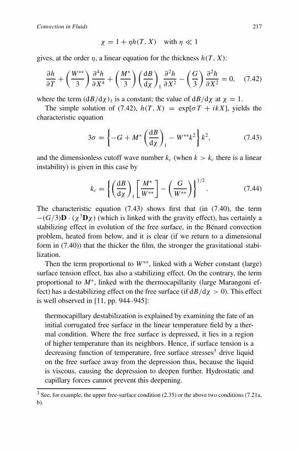
Convection in Fluids 217
χ = 1 + ηh(T ,X) with η � 1
gives, at the order η, a linear equation for the thickness h(T ,X):
∂h
∂T+
(W ∗∗
3
)∂4h
∂X4+
(M∗
3
)(dB
dχ
)1
∂2h
∂X2−
(G
3
)∂2h
∂X2= 0, (7.42)
where the term (dB/dχ)1 is a constant; the value of dB/dχ at χ = 1.The simple solution of (7.42), h(T ,X) = exp[σT + ikX], yields the
characteristic equation
3σ ={−G+M∗
(dB
dχ
)1
−W ∗∗k2
}k2, (7.43)
and the dimensionless cutoff wave number kc (when k > kc there is a linearinstability) is given in this case by
kc ={(
dB
dχ
)1
[M∗
W ∗∗
]−
(G
W ∗∗
)}1/2
. (7.44)
The characteristic equation (7.43) shows first that (in (7.40), the term−(G/3)D · (χ3Dχ) (which is linked with the gravity effect), has certainly astabilizing effect in evolution of the free surface, in the Bénard convectionproblem, heated from below, and it is clear (if we return to a dimensionalform in (7.40)) that the thicker the film, the stronger the gravitational stabi-lization.
Then the term proportional to W ∗∗, linked with a Weber constant (large)surface tension effect, has also a stabilizing effect. On the contrary, the termproportional to M∗, linked with the thermocapillarity (large Marangoni ef-fect) has a destabilizing effect on the free surface (if dB/dχ > 0). This effectis well observed in [11, pp. 944–945]:
thermocapillary destabilization is explained by examining the fate of aninitial corrugated free surface in the linear temperature field by a ther-mal condition. Where the free surface is depressed, it lies in a regionof higher temperature than its neighbors. Hence, if surface tension is adecreasing function of temperature, free surface stresses3 drive liquidon the free surface away from the depression thus, because the liquidis viscous, causing the depression to deepen further. Hydrostatic andcapillary forces cannot prevent this deepening.
3 See, for example, the upper free-surface condition (2.35) or the above two conditions (7.21a,b).

218 The Thermocapillary, Marangoni, Convection Problem
In [11], the authors assume systematically that the Reynolds number of theflow (defined by (7.12) is not too large and use the analogy with Reynold’stheory of lubrication – a general nonlinear evolution equation (as our aboveequation (7.32)) is derived for various particular cases (but, unfortunately,again, in an ad hoc non-rational manner).
When we start from the nonlinear problems (7.30a–c)–(7.31a–c) – withPr = O(1) and R∗ = O(1) fixed – then, as a consequence of the limitingprocess R∗ → 0, time derivatives are dropped, first in equation (7.30a) andthen in equation (7.31a) and we recover the two linear steady-state problems,(7.32a–c) for �0 and (7.35a) with (7.35b) for V0, where the time variableplays the role of a parameter via the thickness χ(T ,X, Y )! Again, one mayask: what is the order of magnitude of time necessary for establishing thevelocity V0 (given by (7.37)) and the dimensionless temperature �0 (givenby (7.32b)) which are both associated with the thickness χ(T ,X)?
The ‘simple’ answer is that: ‘this time for the unsteady adjustment isO(R∗) and that the rate is exponential, the only interesting issue with thispoint being that one need not be anxious about any oscillations which mightpersist without attenuation after the O(Re∗) period’.
Finally, we observe that the linear equation (7.42) for h(T ,X) is a lin-ear Kuramoto–Sivashinsky (KS) equation for small wave amplitude in thelong-wavelength theory and strong surface tension for a relatively largeMarangoni number. In Section 7.5, we derive a nonlinear KS equation andalso an extended KS equation that includes a dispersive term (∂3h/∂x3), aso-called KS–KdV equation. But first we derive an evolution equation à laBenney [14], discovered in 1966, that proved to be succesful in describingthe initial evolution of nonlinear waves.
7.5 Benney, KS, KS–KdV, IBL Model Equations Revisited
In this section we consider mainly the BM thermocapillary convection downa free-falling vertical thin liquid, two-dimensional film, since most experi-ments and theories are linked precisely with such a configuration (see Fig-ure 7.2), the wave dynamics on the free surface of a thin liquid layer alongan inclined plan being quite analogous.
For the case of a convection down a free-falling vertical thin incompress-ible, two-dimensional, liquid film, we work with the dimensionless functions
u = u∗
Uc
, w = w∗
δUc
, p − pA = (p − pA)∗
ρcU 2c
and � = (T − TA)
(Tw − TA)

Convection in Fluids 219
Fig. 7.2 Sketch of a free-falling thin film down along a vertical plane.
and the dimensionless time-space coordinates
t = t∗
(λ/Uc), x = x∗
λ, z = z∗
d, H(t, x) = H ∗
d,
where the ∗ is relative to quantities with dimensions. In terms of these di-mensionless quantities, the dimensionless system of equations and boundaryequations, governing the BM convection problem for a free-falling verticalthin liquid film, becomes
∂u
∂x+ ∂w
∂z= 0; (7.45a)
Du
Dt+ ∂p
∂x− 1
δF 2=
(1
δ Red
)[∂2u
∂z2+ δ2 ∂
2u
∂x2
]; (7.45b)
δ2Dw
Dt+ ∂p
∂z=
(δ
Red
)[∂2w
∂z2+ δ2 ∂
2w
∂x2
]; (7.45c)
PrD�
Dt=
(1
δ,Red
) [∂2�
∂z2+ δ2 ∂
2�
∂x2
]; (7.45d)
• at z = 0:u = w = 0 (7.46a)

220 The Thermocapillary, Marangoni, Convection Problem
and� = 1; (7.46b)
• at z = H(t, x):
∂u
∂z= −δMa
[∂�
∂x+
(∂H
∂x
)∂�
∂z
]− δ2
[∂w
∂x+ 4
(∂H
∂x
)∂w
∂z
]; (7.47a)
p = pA + 2
(δ
Red
) [∂w
∂z−
(∂H
∂x
)∂u
∂z
]− δ2We
∂2H
∂x2
+ δ2
(Ma
Red
) (∂2H
∂x2
)�; (7.47b)
∂�
∂z= −Biconv�+ δ2
[(∂H
∂x
)∂�
∂x− (1/2)Biconv
(∂H
∂x
)2
�
]; (7.47c)
w = ∂H
∂t+ u
∂H
∂x; (7.47d)
where
δ = d
λ, Red = Ucd
νc, Pr = νc
κc, κc = kc
ρcCpc
, F 2 = U 2c
gd, (7.48a)
We = σA
ρcdU 2c
, Ma =(
−dσ
dT
)A
(Tw − TA)
νcρcUc
, Biconv = qconvd
kc.
(7.48b)We note that the upper, deformable free-surface conditions (at z = H(t, x)),(7.47a–c), are written with an error of O(δ3). Below, we first consider thederivation of a Benney type equation.
When δ → 0, we assume that
δ2We = We∗
andRedF 2
= 1 ⇒ Uc = gd2
νc, (7.48c)
and in Biconv we take into account the dependence of the thickness H
Biconv = B(H)
and

Convection in Fluids 221
�∗(H) ≡[
B(H)
(1 +HB(H))
]. (7.49)
As in Benney [14], we write
U = [u,w, p,�]T = U0 + δU1 + O(δ2) when δ → 0, (7.50)
but for the moment we do not expand the thickness of the film, H(t, x) =[1 + ηh(t, x)]. The leading-order solution for U0 is
u0 = −z[(1/2)z −H ]; (7.51a)
w0 = −(1/2)
(∂H
∂x
)z2; (7.51b)
p0 = pA − We∗(∂2H
∂x2
); (7.51c)
�0 = 1 −�∗(H)z. (7.51d)
We get also∂H
∂t+H 2
(∂H
∂x
)= O(δ), (7.51e)
which is a consequence of the evolution equation (see (7.23) and also (4.65))
∂H
∂t+ D ·
(∫ Z=H
0u dZ
)= 0, (7.52)
but written for u0.Using u0, u1, u2, . . . , we may compute q0 and q1 in the expansion of
q(t, x) ≡∫ H(t,x)
0u(t, x, z) dz = q0 + δq1 + δ2q2 + O(δ3). (7.53)
Concerningq0 = (1/3)H 3, (7.54)
which is a consequence of (7.52) with u0 instead of u, being satisfied at theleading order. Concerning q1, we get for u1 a problem similar to problem(7.35a), considered in Section 7.4:
∂2u1
∂z2= Red
{∂u0
∂t+ u0
∂u0
∂x+ w0
∂u0
∂z+ ∂p0
∂x
},
u1 = 0 at z = 0,
this has already been taken into account with (7.51a), the relation (7.51e),

222 The Thermocapillary, Marangoni, Convection Problem
∂u1
∂z
∣∣∣∣z=H(t,x)
= −Ma
[∂�0
∂x+
(∂H
∂x
)∂�0
∂z
]
= Ma�(H)∂H
∂x, (7.55a)
where (see (7.33b))
�(H) ={B(H)+ H
[dB(H)/dH ][1 +HB(H)]2
}. (7.55b)
If we want to take into account the influence of the Prandtl number Pr, as-sumed O(1), then it is necessary to consider for u2 a problem similar to(7.55a, b):
∂2u2
∂z2= Red
{∂u1
∂t+ u0
∂u1
∂x+ u1
∂u0
∂x+ w0
∂u1
∂z+ w1
∂u0
∂z+ ∂p1
∂x
},
u2 = 0 at z = 0,
∂u2
∂z
∣∣∣∣z=H(t,x)
= −Ma
[∂�1
∂x+
(∂H
∂x
)∂�1
∂z
]
−[∂w0
∂x+ 4
(∂H
∂x
)∂w0
∂z
], (7.56a)
but also, for p1 take first into account the problem
∂p1
∂z=
(1
Red
)∂2w0
∂z2,
p1 =(
2
Red
) [∂w0
∂z−
(∂H
∂x
)∂u0
∂z
]at z = H(t, x), (7.56b)
and then, for �1, the following problem:
∂2�1
∂z2= Red Pr
[∂�0
∂t+ u0
∂�0
∂x+ w0
∂�0
∂z
],
�1 = 0 at z = 0 and∂�1
∂z= −Biconv�1 at z = H(t, x). (7.56c)
We note that Red Pr = Pé is the Péclet number.Obviously the determination of the solution of the above second-order
problem (7.56a) for u2, with (7.56b, c), which allows us to take into accountthe (large) Prandtl (Péclet) number effect in a second-order, non-isothermal,

Convection in Fluids 223
à la Benney equation, is rather lengthy, but also especially tedious; it can,however, be used as a good exercise for a ‘plodder’ reader!
The solution for u1 is obtained from (7.55a) when we use the leading-order solution (7.51b–c) and also relation (7.55b) and equation (7.51e) forH , which gives at the leading order: ∂H/∂t = −H 2(∂H/∂x).
Namely we first obtain for u1:
u1 = Red
{We∗ ∂
3H
∂x3[Hz − (1/2)z2] + (1/24)H
(∂H
∂x
)z4
− (1/6)H 2
(∂H
∂x
)z3 + (1/3)H 4
(∂H
∂x
)z
}
+Ma�(H)
(∂H
∂x
)z, (7.57a)
and then
q1 = (1/3)Red
{We∗H 3
(∂3H
∂x3
)+ (2/5)H 6
(∂H
∂x
)}
+ (1/2)MaH 2�(H)∂H
∂x. (7.57b)
Finally, with an error ofO(δ2), we derive the following à la Benney equationfor our thermocapillary convection problem with a variable convection Biotnumber :
∂H
∂x+ H 2 ∂H
∂x+ δ
∂
∂x
{(1/3)Red We∗ H 3
(∂3H
∂x3
)
+ (2/15)H 6
(∂H
∂x
)+ (1/2)Ma
[B(H)
[1 +HB(H)]2
]H 2
(∂H
∂x
)
+ (1/2)Ma
[ [dB(H)/dH ][1 + HB(H)]2
]H 3
(∂H
∂x
) }= 0. (7.58)
In a recent paper by Trevelyan and Kalliadasis [15] concerning inclusionof the Péclet number Pé in an extended à la Benney equation, the authorsassumed that the Péclet number on the right-hand side of the equation forsolution �1 of problem (7.56c) is large so that the convective heat transporteffects are included at a lower relevant order. More specifically, they assumedPé ∼ O(1/δ2/3), and then carried out an expansion in δ up to O(δ4/3), ne-glecting terms of O(δ2) and higher. According to the authors, ‘this level of

224 The Thermocapillary, Marangoni, Convection Problem
truncation allows the derivation of a relatively simple evolution equation forthe free surface as the O(δ2) terms are rather lengthy’, the pressure and tem-perature being both expanded up to O(δ1/3). The reader can find the derivedfree-surface evolution equation (for h(t, x) [15, p. 184, eq. (9)]) and we ob-serve (in spite of fact that the authors write; ‘the seventh term is of O(δ4/3)’)that, on the one hand, this seventh term in their equation (9) appears as pro-portional to δ2 (= δ4/3δ2/3) and, on the other hand, instead of
Pé∗ = δ2/3 Pé = O(1), (7.59)
in a term proportional to δ4/3 as is the case in a rational theory when a sim-ilarity rule, such as (7.59) between small δ and large Pé, is written – in thisseventh term appears again the usual Pé as a term proportional to δ2. How-ever, we observe that, on the contary, in equation (9) of [15], among thefour terms proportional to δ we have as the sixth term of this equation (9):(2/3)δ2 Weh3∂3h/∂x3, and this is justified because, at the start, the authorsassume that We = O(δ2) and δ2 We = O(1). These above various ‘mistakes’introduce ‘confusion’ and it is not clear if the rescaled equation (10) obtainedin [15] is correct, the explanation after this equation being not at all compre-hensible. It is clear that the Benney equation obtained when, at start, Pé isassumed to be a large parameter is certainly not equivalent to a derived (witha Pé fixed – O(1)) extended Benney equation after which Pé is assumed tobe large!
Without the two last terms, proportional to Ma, which take into accountthe Marangoni and also the Biot (convective, via B(H)) effects, the reduced(isothermal) Benney equation,
∂H
∂x+H 2 ∂H
∂x+ δ
∂
∂x
{(1/3)Red We∗H 3
(∂3H
∂x3
)}= 0, (7.60)
has been extensively studied over several decades; see, for instance, [16].This Benney equation (7.60) was also numerically investigated as a partial
first-order differential equation in [17]. However, along with the success ofthis Benney model equation in describing the dynamics of falling liquid film,there is a serious drawback. It turns out that there exists a subdomain in para-meter space, where the Benney equation exhibits solutions whose amplitudegrows without bound and loses its physical relevance (see [18, 19]). In a re-cent paper by Oron and Gottlieb [20], the authors have carried out a bifurca-tion analysis of the first-order Benney equation (7.60) and also of the second-order (in the form given by Lin [21], with several terms proportional to δ2)Benney equation. Recently, alternative and more efficacious approaches that
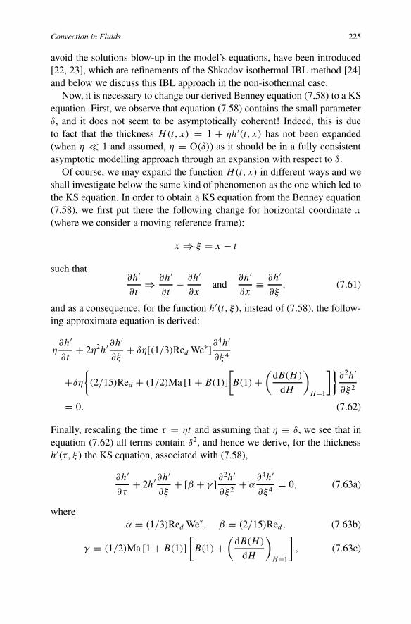
Convection in Fluids 225
avoid the solutions blow-up in the model’s equations, have been introduced[22, 23], which are refinements of the Shkadov isothermal IBL method [24]and below we discuss this IBL approach in the non-isothermal case.
Now, it is necessary to change our derived Benney equation (7.58) to a KSequation. First, we observe that equation (7.58) contains the small parameterδ, and it does not seem to be asymptotically coherent! Indeed, this is dueto fact that the thickness H(t, x) = 1 + ηh′(t, x) has not been expanded(when η � 1 and assumed, η = O(δ)) as it should be in a fully consistentasymptotic modelling approach through an expansion with respect to δ.
Of course, we may expand the function H(t, x) in different ways and weshall investigate below the same kind of phenomenon as the one which led tothe KS equation. In order to obtain a KS equation from the Benney equation(7.58), we first put there the following change for horizontal coordinate x
(where we consider a moving reference frame):
x ⇒ ξ = x − t
such that∂h′
∂t⇒ ∂h′
∂t− ∂h′
∂xand
∂h′
∂x≡ ∂h′
∂ξ, (7.61)
and as a consequence, for the function h′(t, ξ ), instead of (7.58), the follow-ing approximate equation is derived:
η∂h′
∂t+ 2η2h′ ∂h
′
∂ξ+ δη[(1/3)Red We∗]∂
4h′
∂ξ 4
+δη
{(2/15)Red + (1/2)Ma [1 + B(1)]
[B(1)+
(dB(H)
dH
)H=1
]}∂2h′
∂ξ 2
= 0. (7.62)
Finally, rescaling the time τ = ηt and assuming that η ≡ δ, we see that inequation (7.62) all terms contain δ2, and hence we derive, for the thicknessh′(τ, ξ) the KS equation, associated with (7.58),
∂h′
∂τ+ 2h′ ∂h
′
∂ξ+ [β + γ ]∂
2h′
∂ξ 2+ α
∂4h′
∂ξ 4= 0, (7.63a)
whereα = (1/3)Red We∗, β = (2/15)Red, (7.63b)
γ = (1/2)Ma [1 + B(1)][B(1) +
(dB(H)
dH
)H=1
], (7.63c)

226 The Thermocapillary, Marangoni, Convection Problem
with an error of O(δ).An important remark is that, in coefficient γ , given by (7.63c) which takes
into account in the KS equation (7.63a) the influence of the Marangoni ef-fect but also the influence of the Biot effect, we have the constant value ofB(H) and dB(H)/dH , both at H = 1! It seems obvious that B(1) must beidentified with the constant value of the conduction Biot, Bis , number (see,for instance, Section 4.4), the constant value of dB(H)/dH at H = 1 beinga sequel of our starting hypothesis, Biconv = B(H). As a consequence wedo not have the usual (paradoxical) problem related to the cancelling of theMarangoni effect for a vanishing Biot number, since B(1) is certainly differ-ent from zero because it is related to the conduction state! This result justifiesour approach based on a variable convective number and resolves the (false)so-called ‘vanishing Biot problem’!
WithA(τ, ξ) = 2h′(τ, ξ), (7.64)
we obtain, instead of (7.63a), the following canonical KS equation:
∂A
∂τ+ A
∂A
∂ξ+ (β + γ )
∂2A
∂ξ 2+ α
∂4A
∂ξ 4= 0. (7.65)
When α = 0 and (β + γ ) = 0, we obtain the well-known equation
∂A
∂τ+ A
∂A
∂ξ= 0, (7.65a)
and along characteristics (defined by dξ/dτ = A(τ, ξ)) the solutionA(τ, ξ(τ)) is constant.
When α = 0 (We∗ = 0), the surface tension term is removed and (7.65)reduces to Burgers’ equation
∂A
∂τ+ A
∂A
∂ξ+ (β + γ )
∂2A
∂ξ 2= 0. (7.65b)
In this case, the Cole–Hopf transformation further reduces it to the heat equa-tion. Since α > 0 the Cole–Hopf transformation produces a heat equationbackward in time and an initial disturbance will then grow without limit.
Below, we shall include the surface tension term and discuss the fullcanonical KS equation (7.65) or (7.63a), when both α > 0 and β + γ > 0.This full KS equation (7.65) is capable of generating solutions in the form ofirregular fluctuating quasi-periodic waves. The KS model equation providesa mechanism for the saturation of an instability, in which the energy in long-wave instabilities is transferred to short-wave modes which are then dampedby surface tension.

Convection in Fluids 227
In the full KS equation (7.65), the two terms ∂A/∂τ + A∂A/∂ξ , lead tosteepening and wave breaking in the absence of stabilizing terms. The term(β + γ )∂2A/∂ξ 2 destabilizes shorter wave-length modes preferentially andtherefore aggravates wave steepening (since β and γ are both positive). TheBiot effect being usually small, it has no serious influence on this destabi-lization via Marangoni effect. Finally, the term α∂4A/∂ξ 4 is required forsaturation. Unfortunately, explicit analytic solutions of the KS equation arenot available!
A very naïve linear stability analysis shows that, for the KS equation(7.63a), there exists a cutoff wave number. Indeed, if
h′(ξ) ∼ exp[ωτ + ikξ ],then for ω we derive the dispersion relation
ω − (β + γ )k2 + αk4 = 0. (7.66a)
The curve ω = 0 corresponds to neutral linear stability; and in this case thephase velocity, ω/k = c = 0, where the wavenumber k is assumed to bereal, and as a consequence we obtain a ‘cutoff wavenumber’ k∗ such that
(k∗)2 = (β + γ )
α(7.66b)
=(
1
We∗
) {(2/5)+ (3/2)Ma [1 + B(1)]
[B(1)+
(dB(H)
dH
)H=1
]}.
The linear dispersion relation (7.66a) shows that short waves are stable andlong waves are unstable. The critical wavenumber is k∗ = [(β + γ )/α]1/2
which ought to be small for the long-wave analysis to make sense. The max-imum growth rate is (β + γ )2/4α) and occurs at k∗/
√2.
It is anticipated that the effect of the nonlinear (A∂A/∂ξ ) term in thecanonical KS equation (7.65) will be to allow energy exchange between awave with wavenumber k and its harmonics with the end result being non-linear saturation.
The final state may be either chaotic oscillatory motion or a state involv-ing only a few harmonics. The energy equation, corresponding to (7.65), isobtained by multiplying (7.65) by A and integrating by parts, assuming A isperiodic, with period 2L; namely we obtain
(1/2)∂
∂τ
[∫ 2L
0A2 dξ
]=
∫ 2L
0
[(β + γ )
(∂A
∂ξ
)2
− α
(∂A2
∂ξ 2
)2]
dξ.
(7.66c)

228 The Thermocapillary, Marangoni, Convection Problem
The minimization of the right-hand side of (7.66c), over all periodic func-tions, shows that this right-hand side will be negative for π/L > k∗ and,therefore, the nonlinear KS equation (7.65) is globally stable for an initialcondition with a wavenumber satisfying the linear stability criterion.
In other words, if we put in an initial disturbance (e.g., sin(kξ)) with awavenumber k′ greater than k∗, then the nonlinear term in (7.65) createshigher harmonics, but it will not create waves with wavenumbers smallerthan k′, so there will be stability.
If we want to generate a component with a wavenumber in the unstableregion, we have to put in an initial condition with a wavenumber less thank∗. Hence, we need to consider only the case k < k∗. The periodic boundaryconditions allow A to be written as the Fourier series
A =+∞∑−∞
An(τ) exp(inkξ), A−n = A∗n, (7.67)
where A∗n is the complex conjugate of An. Since A0 = const, we may put
A0 = 0 and substitution of (7.67) into the KS equation (7.65) gives thefollowing system of equations:
∂An
∂τ− σnAn + inkBn = 0, (7.67a)
where
Bn =∞∑r=1
A∗rAr+n + (1/2)
n−1∑r=1
ArAn−r , (7.67b)
andσn = (β + γ )(nk)2 − α(nk)4. (7.67c)
The significant feature of the above system of equations (7.67a) with (7.67b,c), is that
for any given k, only a finite number of Fourier modes, say A1, A2, . . . , areunstable (σ1 > 0, σ2 > 0, . . . ), and all higher modes are stable.
Note that the nth mode has a critical wavenumber of k∗/n, and a maximumgrowth rate of [(β+γ )2/4α] – independent of n – at k∗/(n
√2). This implies
that unstable modes will be stabilized by energy transfer to higher harmonics.The simplest case amenable to some theoretical rational analysis is when
k∗
2< k < k∗.

Convection in Fluids 229
Only the n = 1 mode is unstable in this case and in the following it isassumed that it is sufficient to consider just the interaction between n = 1and n = 2 modes. The approximate version of system of equations (7.67a),when we take into account (7.67b), is then (only two equations):
∂A1
∂τ− σ1A1 + ikA2A
∗1 = 0, (7.68a)
∂A2
∂τ− σ2A2 + ik(A1)
2 = 0, (7.68b)
and we note that A1 is unstable (σ1 > 0) but A2 (σ2 < 0) is stable. Note alsothat the following relation is satisfied:
σ1|A1|2 + σ2|A2|2 = 0,
reflecting the required energy balance in the approximate version of
∂
∂τ(�n|An|2) = 2�σn|An|2, n = 1, . . . ,∞,
as a consequence of (7.66c) with (7.67).Equation (7.68a) has the steady solution
|A1| =[−
(1
k2
)σ1σ2
]1/2
, (7.69a)
since from (7.68b),
A2 =(ik
σ2
)(A1)
2. (7.69b)
Here, A1 is growing and A2 is stabilizing. However, as k is decreased, thehypothesis that only two modes are involved becomes more suspect! Indeed,as k is decreased, the steady-state solution of the system of two equations,(7.68a, b), given approximately by (7.69a, b), is at first modified by the pres-ence of a small correction due to A3 and then when
k∗
3< k <
k∗
2(i.e. σ2 > 0, but σ3 < 0),
is replaced by another ‘two-mode equilibrium’ in which A2 and A4 are thedominant components. Further decrease in k then leads to a succession ofstates, alternating between ‘two-mode equilibria’ and ‘bouncy states’. If thesteady solution for A2, given by (7.69b), is substituted into equation (7.68a)then a Landau–Stuart (LS) equation is obtained for A1:

230 The Thermocapillary, Marangoni, Convection Problem
∂A1
∂τ= σ1A1 +
(k2
σ2
)|A1|2A1, (7.70)
and this LS equation (7.70) is, in fact, valid only for k close to k∗. If in (7.70)we assume that A1 = |A1| exp(iϕ), then ϕ = const and for |A1| we derive aclassical Landau equation:
∂|A1|∂θ
= σ1|A1| + λ|A1|3, (7.71)
with λ = (k2/σ2) < 0, since σ2 < 0. The solution of (7.71) is
|A1| ∼ A01 exp(σ1τ) as τ → −∞, (7.72a)
where A01 is the initial value at τ = 0 and σ1 > 0, which decays like the
linearized theory. However,
|A1|2 → −(
2σ1
λ
)as τ → +∞, (7.72b)
for all values of A01; this case is called supercritical stability.
If now we introduce a small perturbation parameter κ , defined by
κ2µ = k2
[(β + γ )
α− k2
]> 0, (7.73)
and a slow time scale T = κ2τ , then for the slowly varying amplitude ofthe fundamental wave H(T ) such that |A1| = κH , from Landau’s equation(7.71), with (7.67c) for σ1 and σ2, we derive the following canonical Landauequation for H(T ):
∂H
∂T= γµH − λH 3, (7.74a)
where the (positive) Landau constant is:
λ = 1/16γ
[k2 −
((β + γ )
4α
)]> 0. (7.74b)
In the above derivation of the Benney equation (7.58) the Reynolds numberRed and also the Marangoni number Ma have been assumed both O(1) andfixed, when in long-wave approximation, the small parameter δ → 0.
Below we consider another case, linked with the low Reynolds and lowMarangoni numbers, which leads to a KS–KdV evolution equation with adispersive additional term, ϕ∂3h′/∂ξ 3.

Convection in Fluids 231
Namely we assume that
Red � 1 and Ma � 1, (7.75a)
such that we have three small parameters and as a consequence we write twosimilarity rules:
Red
δ= Re∗ and
Ma
δ= Ma∗, (7.75b)
with R∗ and M∗ both O(1) and fixed when δ → 0.Again we assume that
δ2 We = We∗ andRed
F 2= 1. (7.75c)
This case, (7.75a–c), leads, instead of (7.58), to an à la Benney evolutionequation, but with some additional terms and then to a modified KS equationwith an additional dispersive term, a so-called KS–KdV equation. With thetwo new constraints (7.75a, b) in the full problem (7.45a–d), (7.46a, b) and(7.47a–d), we obtain the following new problem:
∂u
∂x+ ∂w
∂z= 0, (7.76a)
∂2u
∂z2+ 1 = δ2 Re∗
[Du
Dt+ ∂p
∂x−
(1
Re∗
)∂2u
∂x2
], (7.76b)
∂p
∂z−
(1
Re∗
)∂2w
∂z2= δ2
[(1
Re∗
)∂2w
∂x2− Dw
Dt
], (7.76c)
∂2�
∂z2= δ2
[Pr Re∗ D�
Dt− ∂2�
∂x2
]. (7.76d)
• At z = 0:
u = w (7.77a)
w = 0 (7.77b)
and� = 1. (7.77c)
• At z = H(t, x):
∂u
∂z= −δ2 Ma∗
[∂�
∂x+
(∂H
∂x
)∂�
∂z
]
− δ2
[∂w
∂x+ 4
(∂H
∂x
)∂w
∂z
]+ O(δ4), (7.78a)
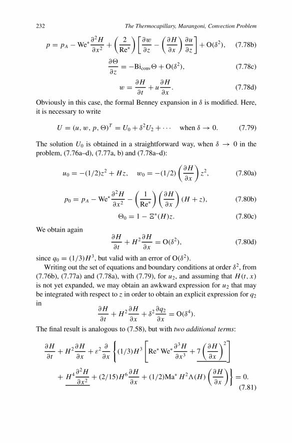
232 The Thermocapillary, Marangoni, Convection Problem
p = pA − We∗ ∂2H
∂x2+
(2
Re∗
)[∂w
∂z−
(∂H
∂x
)∂u
∂z
]+ O(δ2), (7.78b)
∂�
∂z= −Biconv�+ O(δ2), (7.78c)
w = ∂H
∂t+ u
∂H
∂x. (7.78d)
Obviously in this case, the formal Benney expansion in δ is modified. Here,it is necessary to write
U = (u,w, p,�)T = U0 + δ2U2 + · · · when δ → 0. (7.79)
The solution U0 is obtained in a straightforward way, when δ → 0 in theproblem, (7.76a–d), (7.77a, b) and (7.78a–d):
u0 = −(1/2)z2 +Hz, w0 = −(1/2)
(∂H
∂x
)z2, (7.80a)
p0 = pA − We∗ ∂2H
∂x2−
(1
Re∗
) (∂H
∂x
)(H + z), (7.80b)
�0 = 1 −�∗(H)z. (7.80c)
We obtain again∂H
∂t+H 2 ∂H
∂x= O(δ2), (7.80d)
since q0 = (1/3)H 3, but valid with an error of O(δ2).Writing out the set of equations and boundary conditions at order δ2, from
(7.76b), (7.77a) and (7.78a), with (7.79), for u2, and assuming that H(t, x)
is not yet expanded, we may obtain an awkward expression for u2 that maybe integrated with respect to z in order to obtain an explicit expression for q2
in∂H
∂t+H 2 ∂H
∂x+ δ2 ∂q2
∂x= O(δ4).
The final result is analogous to (7.58), but with two additional terms:
∂H
∂t+H 2 ∂H
∂x+ ε2 ∂
∂x
{(1/3)H 3
[Re∗ We∗ ∂
3H
∂x3+ 7
(∂H
∂x
)2]
+ H 4 ∂2H
∂x2+ (2/15)H 6 ∂H
∂x+ (1/2)Ma∗ H 2�(H)
(∂H
∂x
)}= 0.
(7.81)

Convection in Fluids 233
where the function (of H ), �(H), is given above by (7.55b). The evolutionequation (7.81) above, for H(τ, x), is valid with an error of O(δ4). Now,with this evolution equation (7.81) we intend to play the same game as theone considered for the reduction of (7.58) to a KS equation (7.63a).
Thus we use:
τ = δt, ξ = x − t, H = 1 +(
1
ϕ
)δ2h′(τ, ξ) + · · · , (7.82a)
with
η =(
1
ϕ
)δ2, (7.82b)
where ϕ is the dispersive similarity parameter. Carrying out again the limit-ing process δ → 0, we find instead of (7.81) an equation which combinesthe features of the KdV equation on the one hand and the KS equation on theother hand:
∂h′
∂τ+ 2h′ ∂h′
∂ξ+ (β∗ + γ ∗)
∂2h′
∂ξ 2+ ϕ
∂3h′
∂ξ 3+ α∗ ∂4h′
∂ξ 4, (7.83a)
where
β∗ = 2
15ϕ Re∗, α∗ = 1
3ϕ Re∗ We∗, (7.83b)
γ ∗ = 1
2ϕ Ma∗[1 + B(1)]
[B(1) +
(dB(H)
dH
)H=1
], (7.83c)
The evolution KS–KdV equation (7.83a) is again a significant model equa-tion valid for large time with an error of O(δ). The coefficients α∗, γ ∗, β∗and ϕ are all positive constants characterizing dissipation (via Re∗), instabil-ity (via Ma∗), and dispersion (via ϕ), respectively.
As a consequence of the derivation of the KS–KdV equation (7.83a), validfor low Reynolds and Marangoni numbers, we conclude that the features of athin film for a strongly viscous liquid are quite different: the dispersive term,ϕ(∂3h′/∂ξ 3), changes the behavior of the thickness of the liquid film h′(t, ξ )
in space and in time.The above derivation of the KS–KdV model equation was first published
in 1995 [25]. When the dispersion term in equation (7.83a) is zero, this aboveequation reduces to a self-exciting dissipative KS equation which exhibitsturbulent (chaotic) behavior. On the other hand, in the limiting case when Re∗and Ma∗ both tend to zero – a non-viscous liquid film, without the Marangonieffect – equation (7.83a) reduces to the classical KdV equation, well knownin the theory of ‘nonlinear long surface waves in shallow water’, and knownto admit soliton solutions instead of chaos!

234 The Thermocapillary, Marangoni, Convection Problem
Thus, in the general case of non-zero α∗, γ ∗ + β∗ and ϕ, increasing thevalue of ϕ is expected to change the character of the solution of equation(7.83a) from an irregular wave train to a regular row of solitons (a row ofpulses of equal amplitude). The trend is amplified at larger values of ϕ, andthe asymptotic state of the solution for large ϕ takes the form of a row ofthe KdV solitons. There seems to exist a critical value of about unity for thedimensionless parameter:
µ = ϕ
[α∗(β∗ + γ ∗]1/2
which represents the relative importance of dispersion corresponding to thetransition from an irregular wave train to a regular row of solitons.
We note that the complicated evolution of solutions of (7.83a) is describedby the weak interaction of pulses, each of which is a steady-state solution of(7.83a) and when the dispersion is strong, pulse interactions become repul-sive, and the solutions tend, in fact, to form stable lattices of pulses.
The linear dispersion relation of the KS–KdV equation (7.83a) for thewave,
h′(τ, ξ) ≈ exp[ikξ + στ ]is expressed as
σ = (β∗ + γ ∗)k2 − α∗k4 + iϕk3. (7.84a)
For Real(σ ) > 0 we have instability, for Real(σ ) < 0 stability and
Real(σ ) = 0 if k = kc =[(β∗ + γ ∗)
α∗
]1/2
. (7.84b)
Consequently, the cut-off wavenumber for the KS–KdV equation (7.83a) sat-isfies the relation
k2c = (2/5 We∗) + (3/2)
Ma∗
Re∗ We∗ [1 + B(1)][B(1) +
(dB(H)
dH
)H=1
].
(7.84c)Thus waves of small wavenumber are amplified while those of largewavenumber are damped.
To demonstrate the competition between the stationary waves and the non-stationary (possibly chaotic) attractors of the KS–KdV equation (7.83a), weconvert this equation, with α∗ = β∗ + γ ∗ = 1 (with the help of a judiciouschange of function and space-time coordinates) into a finite-dimensional dy-namical system by the Galerkin projection in a periodic medium with wave-length 2π/k:

Convection in Fluids 235
h′(τ, ξ) = (1/2)�Ap(τ) cos(pkξ)+ Bp(τ) sin(pkξ), p > 1. (7.85a)
For a qualitative analysis of projections of the chaotic phase trajectory ontothe plane it seems sufficient to consider a dynamical system truncated at thethird harmonics (as in the Lorenz case). This system can easily be written inan explicit form. First we make a simple linear transformation of the coor-dinates: kξ → x, kτ → t , with the initial condition h′(0, ξ ) = h′0(ξ), andperiodic boundary conditions
h′(τ, ξ) = h′(τ, ξ + 2π/k);the spatial period (wavelength) of the equation is then equal to 2π . Next,substituting (7.85a) into the KS-KdV equation (7.83a), we derive for theamplitudes A1(τ ),B1(t) and B2(t), the following reduced dynamical system:
dA1
dt= σ1A1 + k2ϕB1 − 2A1B2,
dB1
dt= σ1B1 − k2ϕA1 + 2B1B2,
dB2
dt= 2σ2B2 + 2[(A1)
2 − (B1)2], (7.85b)
whereσ1 = k(1 − k2) and σ2 = 2k(1 − 4k2). (7.85c)
The phase flow of the above dynamical system (7.85b) is dissipative if thefollowing relation is satisfied:
σ1 + σ2 < 0,
and because of this dissipative effect, the corresponding strange attractorshave zero phase volume and dimensionality smaller than 3 (when time t
tends to infinity) for the wavenumber k such that 0.58 < k < 1. This three-amplitude DS (7.85b) can be studied qualitatively and numerically.
A final comment concerning the Benney type single evolution equation,which leads in various cases to a non-physical finite-time blow-up (see, forinstance, [18]). The Ooshida regularization procedure [26] of the Benney ex-pansion leads to a single evolution equation for the free surface h that doesnot exhibit this severe drawback – nevertheless, the Ooshida equation failsto describe accurately the dynamics of the film, for moderate Reynolds num-bers, as its solitary wave solutions exhibit unrealistically small amplitudesand speeds. Another single evolution equation including the second-order

236 The Thermocapillary, Marangoni, Convection Problem
dissipation effects was recently introduced by Panga and Balakotaiah [27];in fact, the inertial terms appearing in the model equations offered by bothOoshida and Panga and Balakotaiah can be shown to be equivalent to eachother by using the lowest-order expression ∂h/∂t = −h2∂h/∂x provided bythe flat-film solution and the mass conservation equation. This simple proce-dure was shown to cure the non-physical loss of the solitary wave solutionsand thus to avoid the occurence of finite-time blow-up (see the recent paperby Ruyer-Quil and Manneville [28]).
Concerning the IBL approach, in the isothermal case, this method com-bines the assumption of a self-similar parabolic viscocity profile beneaththe film with the Kármán–Polhausen averaging method used in classicalboundary-layer theory. It seems that this IBL approach was first suggestedby Petr Leonidovitch Kapitza, at the end of the 1940s, to describe stationarywaves and later was extended by Shkadov and coworkers to non-stationaryand three-dimensional films (see [24, 30, 31]). As this is well observed in[9]:
The IBL model does not suffer from the shortcomings of Benney’s ex-pansion and performs well in a region of moderate Reynolds numbersand without any singularities for the solitary wave solution branch.
For the non-isothermal case, Zeytounian [5, 8] first derived an IBL modelconsisting of three averaged equations in terms of the local film thickness(h), flow rate (q) and a function (�) related to the mean temperature acrossthe layer. Later another (more effective) non-isothermal IBL model was pro-posed by Kaliadasis et al. [29]. Finally, more recently, Ruyer-Quil et al. [9]considered the modelling of the thermocapillary flow by using a gradient ex-pansion combined with a Galerkin projection with polynomial test functionfor both velocity and temperature fields and obtained a system of equationsfor h, q and � which is the temperature at the free surface z = h. In [9], amodel consistent at second order is also derived. In [10] the reader can findvarious results of the numerical computation and, in particular, the analysisof the effects of Reynolds, Prandtl and Marangoni numbers on the shape ofwaves, flow patterns and temperature distribution in a film.
In our 1998 paper [8], instead of the upper free-surface condition (7.47c)for �, we used (like other research workers investigating the liquid film flowproblem) the generally accepted, but in fact controversial, Davis [41] condi-tion for the dimensionless temperature θ = (T − Td)/Tw − Td), namely,
∂θ
∂z= −(1 + Bi θ)+ O(δ2) at z = H(t, x);

Convection in Fluids 237
but in fact this has no influence since below we assume that Bi = 0 – theBiot effect being neglected in our 1998 non-isothermal IBL system of threeaveraged equations. For this, with the above θ , instead of (7.48b), we have
We = σd
ρcdU 2c
, Ma =(
−dσ
dT
)d
(Tw − Td)
νcρcUc
and Bi = qd
kc
,
these three parameters (Weber, Marangoni and Biot) being assumed constantin the convection regime.
Below we consider, again, the situation corresponding to a long wave,δ = d/λ � 1 and assume Red � 1, such that δ Red = R∗ = O(1). Inthis case, from equation (7.45c), we obtain the limiting equation ∂p/∂z = 0,when δ → 0 and, according to (7.47b), where instead of δ2 We we haveWe∗ = O(1), we can write, with an error of O(δ2),
p = −We∗ ∂2H
∂x2. (7.86)
With (δ Red = R∗, large Reynolds Red number)
R∗ We∗ = 1
K∗ = O(1),Red
F 2= 1 and δ Ma = M∗∗ = O(1), (7.87)
considering also the large Froude (since Red = F 2) and Marangoni numbers,when δ → 0, we derive at the leading order a reduced ‘boundary layer’ (BL)type two-dimensional problem:
∂u
∂x+ ∂w
∂z= 0, (7.88a)
R∗ Du
Dt− ∂2u
∂z2= 1
δF 2+
(1
K∗
)∂3H
∂x3, (7.88b)
R∗ PrDθ
Dt= ∂2θ
∂z2, (7.88c)
with (when δ → 0) as boundary conditions,
u = w = 0 and θ = 1 at z = 0, (7.89a)
∂u
∂z= −M∗∗
[∂θ
∂x+
(∂H
∂x
)∂θ
∂z
]at z = H(t, x), (7.89b)
∂θ
∂z= −(1 + Bi θ) at z = H(t, x), (7.89c)

238 The Thermocapillary, Marangoni, Convection Problem
w = ∂H
∂t+ u
∂H
∂xat z = H(t, x), (7.89d)
which remains a complicated BL problem very similar to BM long-wavereduced model problem (7.29a–d) formulated in Section 7.3, but formulatedhere for a two-dimensional free-falling vertical film.
When M∗∗ = 0, and in this case the thermal field is decoupled from thedynamical one, Shkadov in 1967 [24], using the integral method, reducedthe above problem to a system of two averaged equations for H(t, x) andq(t, x) = ∫ H
0 u(t, x, z) dz, to use the self-similarity assumption for u,
u(t, x, z) =[U(t, x)
H
]{z − (1/2H)z2}, (7.90a)
where U(t, x) is an arbitrary unknown function, but related to q by
U(t, x) =[
3
H(t, x)
]q(t, x). (7.90b)
In a more general case when M∗∗ �= 0 but Bi = 0 (or Bi/δ = Bi∗ = O(1),the Biot number being usually very small) we can derive two averaged IBLmodel equations for q(t, x) and also for Q(t, x), a function linked with thethermal field
Q(t, x) =∫ H
0[θ(t, x, z) − 1 + z)] dz. (7.91)
Namely we obtain
R∗{∂q
∂t+ ∂
∂x
[∫ H
0u2 dz
]}(∂u
∂z
)z=0
= −M∗∗[∂θ
∂x+
(∂H
∂x
)∂θ
∂z
]+
(1
K∗
)H∂3H
∂x3+H ; (7.92a)
R∗ Pr
{∂Q
∂t+ ∂
∂x
[∫ H
0u[θ(t, x, z) − 1 + z)] dz
]−
∫ H
0w dz
}
+(∂θ
∂z
)z=0
= 0. (7.92b)
With the averaged equation for H(t, x), see (7.52),
∂H
∂t+ ∂q
∂x= 0, (7.92c)

Convection in Fluids 239
an IBL system of three averaged equations (7.92a–c) for three functions H ,q and Q, the Biot number Bi being assumed zero, but the influence of thePrandtl number being taken into account, with Pr = O(1).
Now, with the relations
u(t, x, z) =[U(t, x)
H
]{z − (1/2H)z2} + M∗∗
(∂�
∂x
)z, (7.93a)
θ(t, x, z) − 1 + z = 2
[�(t, x)
H(t, x)
]{z − (1/2H)z2}, (7.93b)
where the function Q(t, x), defined by (7.91), is related to �(t, x) and H by
Q = (2/3)H(H − �), (7.93c)
instead of the averaged equations (7.92a) and (7.92b), we derive our two IBLequations for q(t, x) and �(t, x):
R∗{
∂q
∂t+ (6/5)
∂(q2/H)
∂x+ (1/20)M∗∗ ∂
∂x
[qH
∂�
∂x
]}+
(3
H 2
)q
=(
1
K∗
)H
∂3H
∂x3+ H + (3/2)M∗∗ ∂�
∂x
− (1/120)R∗(M∗∗)2 ∂
∂x
[H 3
(∂�
∂x
)2]
; (7.94a)
∂�
∂t+
[2 −
(�
H
)]∂q
∂x+ (6/5H)
∂
∂x[q(� − H)] + (3/2)
( q
H
) ∂H
∂x
− (9/16H)∂(Hq)
∂x+ M∗∗(1/32H)
∂
∂x
[H 3 ∂�
∂x
]
+ M∗∗(1/40H)∂
∂x
[H 2(� − H)
∂�
∂x
]+ 3
(1
R∗ Pr
) [(� − H)
H 2
],
(7.94b)
and with∂H
∂t+ ∂q
∂x= 0, (7.94c)
we obtain our 1998 IBL non-isothermal system of three averaged equations.In the linear case, when we introduce the perturbations h, ψ and ζ , such
that

240 The Thermocapillary, Marangoni, Convection Problem
H = 1 + δh(t, x), q = (1/3) + δψ(t, x), � = 1 + δζ(t, x), (7.95)
from (7.94a–c) we derive, with ∂ψ/∂x = −∂h/∂t , for the perturbations, hand ζ , the following linear system of two equations:
∂2h
∂t2+ (4/5)
∂2h
∂t∂x+ (2/15)
∂2h
∂x2+ We∗ ∂
4h
∂x4
+(
3
R∗
) [∂h
∂t+ ∂h
∂x
]+ (3/2)
(M∗∗
R∗
)∂2ζ
∂x2
−(M∗∗
60
)∂3ζ
∂x3= 0, (7.96a)
∂ζ
∂t− (7/16)
∂h
∂t+ (2/5)
∂ζ
∂x− (7/80)
∂h
∂x+
(M∗∗
32
)∂2ζ
∂x2
+(
3
R∗ Pr
)(ζ − h) = 0. (7.96b)
In Section 7.6, devoted to various aspects of the linear and weakly nonlinearstability analysis of the thermocapillary convection, the above system (7.96a,b) is investigated in the framework of infinitesimal disturbances.
7.6 Linear and Weakly Nonlinear Stability Analysis
As our first example we consider a linear stability analysis of the clas-sical BM two-dimensional (as in [32]) problem when, again, instead ofthe dimensionless temperature �, we use the dimensionless temperatureθ = (T − Td)/Tw − Td). In this linear case, from our ‘correct’ upper, free-surface dimensionless condition for θ (1.24c), at z = H = 1 + ηh(t, x), wecan write
∂θ
∂n′ +[
Biconv
Bis(Td)
]{1 + Bis(Td)θ} = 0,
when Q0 = 0. Because in the conduction case, θs(z) = 1 − z, we write:
θ = 1 − z + ηθ ′ + · · · and Biconv = B(H) = B(H)+ ηh
(dB
dH
)H=1
,
with B(H) ≡ Bis as the conduction Biot number.

Convection in Fluids 241
From the above upper free-surface condition, written at z = 1, and theexpansion for θ and Biconv, we first obtain
−1 + ∂θ ′
∂z+
[1 + η
(1
Bis
) (dB
dH
)H=1
h
]{1 + η Bis[θ ′ − h]} = 0,
and as a consequence at the order η, we derive the following linearized uppercondition (at z = 1):
∂θ ′
∂z
∣∣∣∣z=1
+ Bis[h − θ ′z=1] +
(1
Bis
) (dB
dH
)H=1
h = 0. (7.97)
If the last (third) term on the left-hand side of (7.97) can be assumed tobe zero, this is not the case for the second term proportional to conductionconstant Biot number Bis .
Below, if we want to use the Takashima classical linear theory [35], thenas condition we choose, neglecting the term (1/Bis)(dB/dH)H=1h,
∂θ ′
∂z
∣∣∣∣z=1
+ Bis[h − θ ′z=1] = 0, (7.98)
which is the Takashima condition but with Bis �= 0 as Biot number. Ob-viously, the general case (with the term (1/Bis)(dB/dH)H=1h) deservesconsideration. With (7.98) the various results of Takashima are correct, forBis �= 0; on the contrary, the Takashima results for (the Takashima) Biotnumber = 0 are questionable! As a basic steady-state solution we have
uBM = 0, πBM = 0, θBM = 1 − z and H = 1.
For a two-dimensional case, Takashima assumes that in the linearized (η �1) BM problem, the perturbations u′, w′, π ′ and θ ′ are decomposed in termsof normal modes (with h0 = const):
(u′, w′, π ′, θ ′, h) = [U(z),W(z), P (z), T (z), h0] exp[σ t + ikx]. (7.99)
As in Takashima’s example, two linear OD equations are derived:
{σ −
[d2
dz2− k2
]}[d2W
dz2− k2W
]= 0, (7.100a)
{Pr σ −
[d2
dz2− k2
]}T = Pr W, (7.100b)
with linear conditions

242 The Thermocapillary, Marangoni, Convection Problem
dW
dz
∣∣∣∣z=0
= 0, W(0) = 0, T (0) = 0; (7.100c)
d2W
dz2
∣∣∣∣z=1
+ k2W(1) + k2 Ma[T (1) − h0] = 0; (7.100d)
[σ + 3k2] dW
dz
∣∣∣∣z=1
− d3W
dz3+ k2
[(1
Fr2Ad
)+ k2We
]h0 = 0; (7.100e)
dT
dz
∣∣∣∣z=1
+ Bis[T (1) − h0] = 0; (7.100f)
W(1) = σh0. (7.100g)
The problem (7.100a–g) is our eigenvalue (linear) problem, and Takashimaconsidered two cases: (1) σ = 0, when the neutral state is a stationary one,and (2) σ �= 0, when we have ‘overstability’. In case (1), the general solu-tion of the two equations (7.100a, b), with σ = 0, for W(z) and T (z), caneasily be obtained through the sinh(kz) and cosh(kz); when these solutionsare substituted into the boundary conditions (7.100c–g), then we derive thefollowing eigenvalue relationship:
Ma = 8k[sinh(k) cosh(k)− k][k cosh(k)+ Bis sinh(k)](Bd + k2)
8Cr∗ k5 cosh(k)+ (Bd + k2)[sinh3(k)− k3 cosh(k)](7.101)
which is a result derived in [32]. In [33] the growth rate of disturbances forthe non-zero mode is also studied. For fixed values of Bis , Bd = Pr Cr∗/Fr2
Ad
and Cr∗ = 1/Pr We, relation (7.101) enables us to plot the stability curve inthe (k; Ma)-plane (see the figures in [32, pp. 2748, 2749]). In particular,when Bd > 0 (the case when the upside of the liquid layer is a free surface),the values of Cr∗ are given in [32, fig. 1, p. 2748]: since the region beloweach curve represents a stable state, the lowest point of each curve gives thecritical Marangoni number Mac and the corresponding critical wave numberkc. It follows that Ma has a minimum value at k = 0. The values of Macand kc, when Cr∗ < Bd/120, are almost independent of Bd and Cr∗ and arealmost the same as those obtained by Pearson [34] in 1958. In such a casethe free surface deformation is not important and therefore the assumption ofa non-deformable free surface is valid. The condition under which the free-surface deformation becomes important can be expressed as (see also ourcondition (1.11)),
d < d∗ =[
120νκ
g
]1/3
. (7.102)

Convection in Fluids 243
For water, d∗ = 0.012 cm. We observe also that for kc = 0 we have, fromproblem (7.100a–g), that W = 0 and there can be no motion. In practice,however, the presence of lateral boundaries will impose a non-zero lowerbound on the horizontal wave number, and the minimum Marangoni numberrequired to cause convection will be raised (see, for instance [35]).
In case (2), considered in [32, pp. 2751–2756], again the general solutionsof problem (7.100a, b), with σ �= 0, can be obtained and these, when substi-tuted into (7.100c–g), yield a time-dependent eigenvalue relationship of theform
Ma = L(Bis , Bd,Cr∗,Pr, k, σ ), (7.103)
where L is a real-valued function of parameters in parentheses. The neutralstability curves for the onset of overstability (the alternative possibility of theinstability setting in as oscillations) lie only in the negative region of Ma and,contrary to the case of a stationary mode, the region above each curve in [32,fig. 2, p. 2754] represents a stable state. The highest point of each curve givesthe critical Marangoni number Mac for the onset of overstability and thecorresponding critical wave number kc. In fact, the free surface deformationmust be taken into account when (for Bd > 0) Ma > 0 and 120Cr∗ > Bd >
0, or Ma < 0 and Bd > 0, and when Ma < 0 the liquid layer can becomeunstable via a marginal state of purely oscillatory motions. It is thereforeconcluded that, when the upside of the liquid layer is a free surface (Bd > 0),instability is possible for heating in either direction, but the manner of theonset of instability depends on the direction of heating.
Concerning now the KS-KdV equation (7.83a), another way for thederivation of a three-amplitude DS (different from (7.85b)) is the Fourierseries. In this case we assume that
h(τ, ξ) = (1/2)�An(τ) exp[in(ω01τ − k1ξ)], (7.104a)
where An(τ) is the complex amplitude of the n-th spatial harmonic, andwhere ω0
1 is the linear angular frequency (in fact, the angular frequency ofthe fundamental harmonic, with k1 as wavenumber, at the first stage of itsgrowth). It must be stressed that, if the wavenumber kn = nk1 is the ac-tual wavenumber of the n-th harmonic, the frequency nω0
1, on the contrary,cannot be considered as its actual frequency ωn; the latter may vary a little,owing to possible small dispersive effects. The slow variation ψn(τ) of thephase corresponding to this small frequency shift is taken into account in thecomplex amplitude
An(τ) = |An(τ)| exp[iψn(τ)]. (7.104b)

244 The Thermocapillary, Marangoni, Convection Problem
Inserting (7.104a) into equation (7.83a), for the first three harmonics we de-rive the following three-amplitude DS (again, with α∗ = 1 and β∗+γ ∗ = 1):
dA1
dτ= γ1A1 + ik1A
∗1A2, (7.105a)
dA2
dτ= (γ2 − 6ik3
1ϕ)A2 + ik1A21, (7.105b)
dA3
dτ= (γ3 − 24ik3
1ϕ)A3 + 3ik1A1A2, (7.105c)
whereγn = (nk1)
2[1 − (nk1)2], n = 1, 2, 3. (7.105d)
Near criticality, where the mode A1 is the only unstable mode, while theothers are linearly strongly damped, the dynamics are controlled by the mar-ginally unstable mode A1, to which the other two modes are slaved. As aconsequence, from (7.105b), we have that the dynamics of the harmonics A2
is slaved to the dynamics of the fundamental harmonic, A1, according to
A2 = −[
ik1
(γ2 − 6ik31ϕ)
]A2
1. (7.106)
From (7.105a), with (7.106), the fundamental harmonic A1 obeys the follow-ing Stuart–Landau type equation:
dA1
dτ= γ1A1 + λA∗
1A21, (7.107a)
where
λ =(
γ2k21
a2
)[1 + i(6k3
1ϕ)
γ2
], (7.107b)
with a2 = γ 22 + 36k6
1ϕ2, and γ2 > 0.
The real part (positive) of the complex Landau constant λ corresponds tononlinear dissipation, and its imaginary part to nonlinear frequency correc-tion (due to dispersive effects). The dispersive character of the waves playsa crucial role (via the parameter ϕ in (7.83a)) in the occurence of amplitudecollapses and frequency locking.
This may be understood within the framework of the above DS (7.105a–c)after separation of modulus and phase of the complex amplitudes (accordingto (7.104b)).
For the simple case of |A1(τ )| and |A2(τ )| and phase difference �(τ) =ψ2 − 2ψ1, we derive the following DS of three equations instead of (7.105a–c):

Convection in Fluids 245
d|A1|dτ
= γ1|A1| − k1|A1| |A2| sin �, (7.108a)
d|A2|dτ
= γ2|A2| + k1|A1|2 sin �, (7.108b)
d�
dτ= −6(k1)
3ϕ + k1
{ [|A1|2 − 2|A2|2]|A2|
}cos �, (7.108c)
which is a particular case of the more complicated DS considered in [36] anddeserves a further careful numerical investigation.
We return to the system of two linear equations (7.96a, b) which are de-duced from our IBL system (7.94a–c) in Section 7.5. These two equationsalso certainly deserve further careful investigation. Here we will consideronly a particular case when Pr is vanishing, Pr → 0, and in a such case theequation (7.96b) leads to ζ = h. As a consequence, in this particular case,from (7.96a) we obtain the following single linear equation for the thicknessof the film h(t, x):
∂2h
∂t2+ (4/5)
∂2h
∂t∂x+
[(2/15) + (3/2)
(M∗∗
R∗
)]∂2h
∂x2
−(
M∗∗
60
)∂3h
∂x3+ We∗ ∂4h
∂x4+
(3
R∗
) [∂h
∂t+ ∂h
∂x
]= 0. (7.109)
This evolution equation, with the parameters M∗∗, R∗ and We∗ is, in fact, anevolution equation for the deformation of the free surface which generalizesthe KS–KdV classical equation.
Whenh(t, x) ≈ exp[ik(x − ct)],
we obtain as dispersion equation(
3
R∗
)[c − 1] − ik[c2 − (4/5)c + (2/5)] + ik3We∗
=(
M∗∗
2
) [(1/30)k2 + i
(3
R∗
)k
], (7.110)
and if c = cr + ici , with k real, we obtain two equations for real and imagi-nary parts:
(3
R∗
)[1 − cr ] + kci[(4/5) − 2cr ] +
(M∗∗
60
)k2 = 0, (7.111a)

246 The Thermocapillary, Marangoni, Convection Problem(3
R∗
)ci −
[c2r − c2
i − (4/5)cr + (2/15) + (3/2)
(M∗∗
R∗
)]k+k3 We∗ = 0.
(7.111b)If ci > 0, the disturbances are amplified, while if ci < 0, the disturbancesare vanishing. When ci = 0 in (7.111a), then for the phase velocity corre-sponding to a neutral disturbance, we obtain the following relationship:
c∗r ≡ c∗ = 1 + (1/180)M∗∗ R∗k2. (7.112)
As a consequence, when M∗∗ �= 0, it appears that the infinitesimal pertur-bances are dispersives. If we introduce
B∗ ≡ (1/180)M∗∗ R∗,
then from (7.111b), when ci = 0 and with (7.112) we obtain for the determi-nation of the cut-off (neutral) wavenumber kc (�= 0) the following equation:
B∗(k2c )
2 + [(6/5)B∗ − We∗]k2c + (1/3) + (3/2)
(M∗∗
R∗
)= 0, (7.113)
and when M∗∗ �= 0, B∗ �= 0 and if
We∗ ≥ (6/5)B∗ + 2B∗[(1/3) + (3/2)
(M∗∗
R∗
)]1/2
, (7.114a)
then we have, for k2c , one or two positive values. A particular case which
leads to a single value for k2c is
k2c =
(1
B∗
)[(1/3) + (3/2)
(M∗∗
R∗
)]1/2
, (7.114b)
and this is the case, when in space parameters (We∗,M∗∗, R∗) the followingrelationship is justified:
(30
M∗∗ R∗
)We∗ = (1/5) + (1/3)
[(1/3) + (3/2)
(M∗∗
R∗
)]1/2
. (7.114c)
When k > kc, the disturbances are vanishing and for k < kc, the distur-bances are unstable. We observe that from the relation (7.113) we obtain arelationship for M∗∗ as a function of We∗ and R∗:
M∗∗ = k2c We∗ − (1/3)
(3/2)(1/R∗) + (1/180)R∗k2c [k2
c + (6/5)] (7.115)

Convection in Fluids 247
and M∗∗ > 0 ifkc > (1/3 We∗)1/2. (7.116a)
When M∗∗ = 0, the condition for a neutral stability, ci = 0 (and in a suchcase also cr ≡ 1), is
kc = (1/3 We∗c)
1/2 (7.116b)
and we have linear stability (k > kc) for
We∗ > We∗c ≡ (1/3k2
c ). (7.116c)
When k < kc we have linear instability and in this case, ci > 0 and cr ≡ 1.If we consider both equations (7.96a) and (7.96b) for the functions ζ(t, x)
and h(t, x) and assume that
h(t, x) ≈ h0 exp[ik(x − ct)] and ζ(t, x) ≈ ζ 0 exp[ik(x − ct)],then instead of the single equation (7.110) we derive the following dispersionrelation: (
3
R∗
)[c − 1] − ik[c2 − (4/5)c + (2/5)] + ik3We∗
=[B
A
] (M∗∗
2
)[(1/30)k2 + i
(3
R∗
)k
], (7.117a)
with [B
A
]= 3(1/PrR∗) + (7/16)ik[c − (1/5)]
3(1/PrR∗)− (1/32)M∗∗k2 − ik[c − (2/5)] , (7.117b)
and unless the case of Pr = 0 (and in a such case [B/A] = 1), the ratio[B/A] is a complex function of k and c and the dispersion relation (7.117a)is very complicated, a numerical computation certainly being necessary.
The above very concise linearized stability theory gives very limited re-sults concerning instability, because the amplitude of the disturbance isfound to grow exponentially in time for values of certain flow parametersabove a critical value.
In reality, such disturbances do not grow exponentially without limit, andan at least weakly nonlinear stability (WNS) analysis is obviously a neces-sary task! In this WNS theory the Landau–Stuart (LS) equation plays an im-portant role. As a simple example, we consider the Shkadov IBL isothermalmodel with two equations (7.92c) and (7.92a) for h and q but with M∗∗ = 0;for the details of the derivation the reader can turn to our survey paper [8].

248 The Thermocapillary, Marangoni, Convection Problem
The main small parameter, using a multiscale technique, is η whichis a measure for the deformation of the upper free-surface z = H (≡1 + ηh(t, x, y)) and as bifurcation parameter we choose the modified Webernumber We∗ such that
We∗ = We∗c + Sη2, (7.118a)
where S is a scalar assumed O(1); as η � 1, we are interested in a weaklynonlinear stability analysis, near neutral stability. For the phase velocity wewrite
cr = c∗r + c2η
2 with c∗r = 1, (7.118b)
and we introduce slow coordinates
ξk = ηkξ, ξ = (x − cr t), k = 0, 1, 2, . . . (7.118c)
In reality, if we want to derive the LS envelope equation, it is sufficient toassume that the amplitude of the wave packet envelope is only a function ofξ 2 ≡ X. Now, for the functions h(t, x) and q(t, x) we consider the expan-sion:
h = h′(ξ,X; η) = 1 + ηh1 + η2h2 + η3h3 + · · · , (7.119a)
q = q ′(ξ,X; η) = (1/3) + ηq1 + η2q2 + η3q3 + · · · . (7.119b)
According to linear theory,
h1(ξ,X) = A(X)E(ξ)+ A∗(X)E(−ξ), (7.120a)
with E(±ξ) = exp(±ikcξ), where kc is the neutral (cut-off) wavenumberand A∗ the complex conjugate of the amplitude A (AA∗ = |A|2).
For the derivation of the LS equation for the amplitude A(X) of the wave-packet envelope, it is necessary to eliminate the secular terms in the equa-tions for h3(ξ,X) and q3(ξ,X), assuming that the asymptotic expansions(7.119a, b) are uniformly valid with respect to the coordinate ξ . Next, takinginto account the relations
∂
∂t= −cr
(∂
∂ξ+ η2 ∂
∂X
)and
∂
∂x= ∂
∂ξ+ η2 ∂
∂X, (7.120b)
we substitute the expansions (7.119a, b) and (7.117a, b) for We∗ and cr intoequations (7.92c) and (7.92a), for h and q, but with M∗∗ = 0. By identifi-cation of the terms in different orders of η, up to 3, we derive a sequence ofdifferential equations. The solution of these differential equations is straight-forward. If we introduce the operator

Convection in Fluids 249
�(h, q) ≡ −(1/5)∂q
∂ξ−(2/15)
∂h
∂ξ+
(3
R∗
)[q−h]−(1/3k2
c )∂3h
∂ξ 3, (7.121)
then we derive successively the following solutions: first
h1(ξ,X) = A(X)E(ξ)+ A∗(X)E(−ξ), (7.122a)
q1(ξ,X) = A(X)E(ξ)+ A∗(X)E(−ξ), (7.122b)
thenh2(ξ,X) = q2(ξ,X)− 2|A(X)|2, (7.122c)
q2(ξ,X) = β|A(X)|2E(2ξ) + β∗|A∗(X)|2E(−2ξ), (7.122d)
withE(±2ξ) = exp(±2ikcξ)
and
β = −[(7/10) + i(3/2kcR∗)], β∗ = −[(7/10) − i(3/2kcR
∗)].At the third order, there appears first the equation
�(h3, q3) = γ |A∗(X)|3E(3ξ)
+[−(2/3)
dA
dX+ λA(X)− µA(X)|A∗(X)|2
]E(ξ)+ c.c.
and also, for h3, the relation
h3 = q3 − c2h1.
The solution for q3 is of the form
q3 = D(A)E(3ξ)−{(3/2)
[κc2A+ (2/3)
dA
dX−λA(X)
+ µA(X)|A(X)|2]E(ξ)
}ξ + c.c., (7.122e)
and, in (7.122e), the term underlined in { } before ξ , is a ‘secular term’, whichis very large with increasing ξ !
As a consequence, this term η3q3, in (7.119b) may not be small relative tothe term η2q2! Finally, by elimination of this secular term, we derive our LSequation:

250 The Thermocapillary, Marangoni, Convection Problem
(2/3)dA
dX+ νA+ µA(X)|A(X)|2 = 0. (7.123)
In the LS equation (7.123), the coeficients ν and µ are given by
ν = κc2 − λ =(
3
R∗
)c2 + i[−(6/5)kcc2 + Sk3
c ], (7.124a)
µ =(
93
10R∗
)+ i
[(31/50)kc +
(9
kc
)(1
R∗
)2]. (7.124b)
For the determination of c2, we can assume that the coeficient ν is real and,in such a case,
c2 = (5/6)Sk2c , (7.124c)
and, instead of (7.123), we obtain for the amplitude A = A(X), the LSequation
−dA
dX= αSA+ (3/2)µA|A|2 (7.125a)
with
α = (15/4)
(1
R∗
)k2c . (7.125b)
From (7.125a) it is judicious to derive a Landau classical equation for theamplitude A, with real coefficient αS and µr = (93/10R∗). For this thecomplex amplitude A(X), a solution of the above LS equation (7.125), whereµ = µr + iµi , is written as
A(X) = |A(X)| exp[i�(X)], (7.126a)
and for |A(X)| we derive, from (7.125a), the Landau equation
d|A|(X)|dX
= −αS|A(X)| − (3/2)µr |A|3. (7.126b)
For the phase �(X) we obtain the relation
d�(X)
dX= −(3/2)µi |A(X)|2, (7.126c)
with
µi = (31/50)kc +(
9
kc
)(1
R∗
)2
. (7.126d)
The above Landau equation (7.126b) implies that the solution |A| = 0 is anequilibrium solution which is stable if

Convection in Fluids 251
We∗ < We∗c ,
or unstable ifWe∗ > We∗
c ,
respectively, and |A| → |A|c is a new equilibrium value as X → −∞. Thebranching of the curve of the equilibrium solution |A| = 0 at We∗ = We∗
c iscalled the Landau bifurcation. When We∗ > We∗
c , then S > 0 so that
−d|A(X)|dX
> 0 and |A|(X)increases exponentially as X → −∞.
This case corresponds to a rapid transition to turbulence (chaos). The Landauequation (7.125b) is, in fact, an OD linear equation,
dL(X)
dX− 2αSL(X) = 3µr, (7.127a)
for the function
L(X) =[
1
|A(X)|2], (7.127b)
and as a consequence, we may solve (7.127a) explicitly. Using this explicitsolution we may estimate the critical rupture X = Xc, corresponding toL(Xc) = 0. Concerning the nonlinear rupture of the films, the reader canfind various useful information in a paper by Erneux and Davis [40].
Obviously, it is necessary to consider such a theory as above, for the non-isothermal case when, instead of Shkadov’s IBL system (7.92c), (7.92a), weinvestigate the weakly nonlinear stability of the IBL system with three equa-tions, (7.92c) with (7.96a) and (7.96b). Obtaining such an amplitude equa-tion from these non-isothermal three equations is a good working example,and can also be performed for a non-isothermal system of three equationsderived, respectively, in [29], [9] and [10]; in Section 10.4, we discuss thederivation of some non-isothermal systems of three equations obtained inthe papers cited above. On the other hand, in Section 10.5, the reader canfind a discussion concerning a paper published by Golovin et al. (in 1994)[37] relative to ‘Interaction between short-scale Marangoni thermocapillaryconvection and long-scale deformational instability’, with some commentson the numerical results of Kazhdan [38] obtained via a three amplitude DS.
Finally, we observe that for the lubrication equation (7.40) derived inSection 7.4, as in [39] for example, we can (at least in the unsteady one-dimensional case, see (7.41) use the concept of a Liapounov function andderive the corresponding conservation law; on the other hand the existence

252 The Thermocapillary, Marangoni, Convection Problem
of a Liapounov function (decreasing function along any trajectory) providesa start for any meaningful nonlinear stabity analysis of equation (7.41). Werecall that if a system has a Liapounov functional bounded from below (a freeenergy functional), then any initial data evolve into a steady state.
7.7 Some Complementary Remarks
We begin with the formulation of a second (modified) model problem for theBM thermocapillary convection, for the function
u′, π and θ = (T − Td)
(Tw − Td)(7.128)
instead of
u′, π and �
[= (T − TA
(Tw − TA)
],
which are solutions of the model problem (7.6a–c), (7.7a, b) and (7.8a–e) inSection 7.2.
In such a case, according to the discussion in Chapter 1 relative to theupper free-surface condition (1.38), for the dimensionless temperature θ , wetake into account, instead of (7.8d), just this condition (1.38) which seemssimilar to the Davis condition derived in [41], but different owing to the factthat in (7.38) we have the convection Biot number Biconv instead of Bis , theconduction Biot number in the Davis condition.
We have again (with ε, the expansibility parameter given by (1.10a)),Fr2
d, ≈ 1 and, as a consequence, Gr ≈ ε � 1. For the functions u′, πand θ as model equations, we obtain (unless prime for uBM):
∇ · uBM = 0, (7.129a)
duBM
dt+ ∇πBM = �uBM, (7.129b)
PrdθBM
dt= �θBM, (7.129c)
where
Pr = ν(Td)
κ(Td)with κ(Td) = k(Td)
ρ(Td)Cv(Td).
At z = 0, we haveuBM|z=0 = 0 (7.130a)

Convection in Fluids 253
andθBM|z=0 = 1. (7.130b)
For the leading-order BM equations (7.129a–c), as associated leading-orderupper conditions for πBM|z=H we have:
πBM =(
1
Fr2d
)(H − 1)+
(2
N
){(∂u1BM
∂x
) (∂H
∂x
)2
+(∂u2BM
∂y
)(∂H
∂y
)2
+ ∂u3BM
∂z+
[∂u1BM
∂y+ ∂u2BM
∂x
](∂H
∂x
)(∂H
∂y
)
−[∂u1BM
∂z+ ∂u3BM
∂x
] (∂H
∂x
)−
[∂u2BM
∂z+ ∂u3BM
∂y
] (∂H
∂y
)}
−(
1
N
)3/2
[We − Ma θBM]{N2
(∂2H
∂x2
)
− 2
(∂H
∂x
)(∂H
∂y
)(∂2H
∂x∂y
)+N1
(∂2H
∂y2
)}at z = H(t, x, y),
(7.131a)
where, according to (1.18a, b),
We = σdd
ρdν2d
,
Ma = γσd�T
ρdν2d
,
with �T = Tw − Td , and we observe that in the first BM model (see (7.8a),in the definition of Ma, instead of �T , we have the temperature difference(Tw − TA), this is also the case for the expansibility small parameter ε!
Then, instead of the two tangential upper free-surface conditions (7.8b, c),with Marangoni effect, we have
[∂u1BM
∂x− ∂u3BM
∂z
] (∂H
∂x
)+ (1/2)
[∂u1BM
∂y+ ∂u2BM
∂x
] (∂H
∂y
)
+ (1/2)
[∂u2BM
∂z+ ∂u3BM
∂y
] (∂H
∂x
)(∂H
∂y
)
− (1/2)
[1 −
(∂H
∂x
)2] [
∂u3BM
∂x+ ∂u1BM
∂z
]
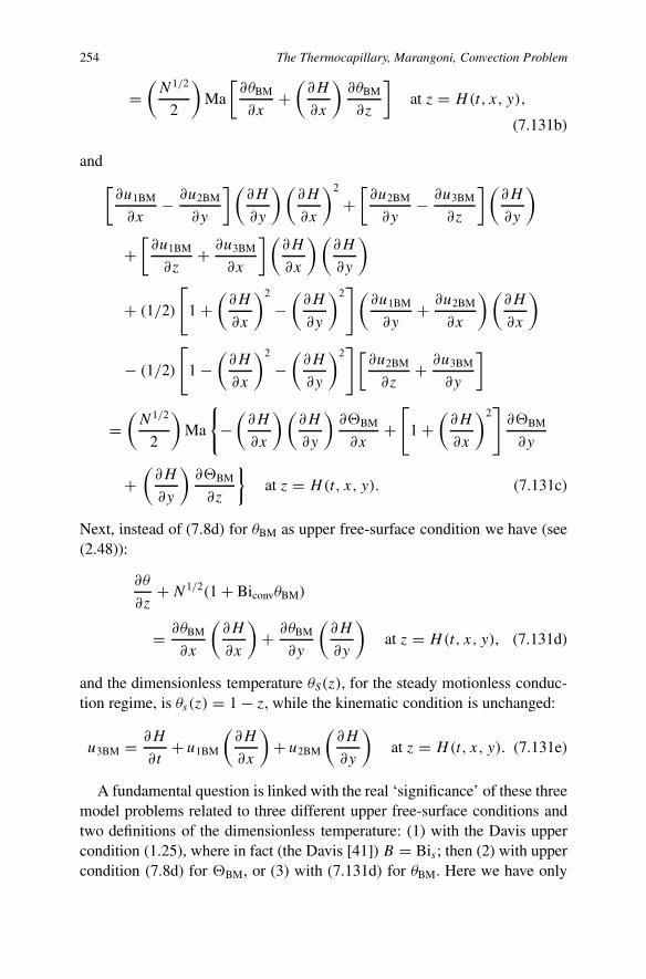
254 The Thermocapillary, Marangoni, Convection Problem
=(N1/2
2
)Ma
[∂θBM
∂x+
(∂H
∂x
)∂θBM
∂z
]at z = H(t, x, y),
(7.131b)
and[∂u1BM
∂x− ∂u2BM
∂y
] (∂H
∂y
) (∂H
∂x
)2
+[∂u2BM
∂y− ∂u3BM
∂z
](∂H
∂y
)
+[∂u1BM
∂z+ ∂u3BM
∂x
] (∂H
∂x
) (∂H
∂y
)
+ (1/2)
[1 +
(∂H
∂x
)2
−(∂H
∂y
)2](
∂u1BM
∂y+ ∂u2BM
∂x
) (∂H
∂x
)
− (1/2)
[1 −
(∂H
∂x
)2
−(∂H
∂y
)2][
∂u2BM
∂z+ ∂u3BM
∂y
]
=(N1/2
2
)Ma
{−
(∂H
∂x
) (∂H
∂y
)∂�BM
∂x+
[1 +
(∂H
∂x
)2]∂�BM
∂y
+(∂H
∂y
)∂�BM
∂z
}at z = H(t, x, y). (7.131c)
Next, instead of (7.8d) for θBM as upper free-surface condition we have (see(2.48)):
∂θ
∂z+N1/2(1 + BiconvθBM)
= ∂θBM
∂x
(∂H
∂x
)+ ∂θBM
∂y
(∂H
∂y
)at z = H(t, x, y), (7.131d)
and the dimensionless temperature θS(z), for the steady motionless conduc-tion regime, is θs(z) = 1 − z, while the kinematic condition is unchanged:
u3BM = ∂H
∂t+ u1BM
(∂H
∂x
)+ u2BM
(∂H
∂y
)at z = H(t, x, y). (7.131e)
A fundamental question is linked with the real ‘significance’ of these threemodel problems related to three different upper free-surface conditions andtwo definitions of the dimensionless temperature: (1) with the Davis uppercondition (1.25), where in fact (the Davis [41]) B = Bis; then (2) with uppercondition (7.8d) for �BM, or (3) with (7.131d) for θBM. Here we have only

Convection in Fluids 255
to bring attention to this question and we do not have to give any definitiveanswer!
Still the fact remains that, personally, I think the model problem with �BM
(case (2)) for the BM thermocapillary convection (considered in Section 7.2)is a fundamentally rational model, where the difference between conductionregime (with Bis(TA) and �S(z)) and convection regime (with a variableBiconv and the dimensionless temperature �BM) is clearly taken into account!But, on the other hand, the model problem (case (3) with θBM) for the BMthermocapillary convection allows us to use classical results derived with thehelp of the Davis (case (1)) upper condition, changing B (= Bis) to Biconv.
However, here it seems necessary to note a ‘negative’ aspect of the BMmodel with �BM (see Section 2.5) linked with the fact that, when we usethe dimensionless temperature �, when the difference of temperature Tw −TA appears, then we are constrained to write for the temperature-dependentsurface tension σ (T ) the approximate relation
σ (T ) = σ (TA)
[1 −
(Ma
We
)�BM
],
with
Ma =[−dσ (T )
dT
]A
d(Tw − TA)
ρ(TA)ν(TA)2
where in Ma we have also Tw − TA, and in reality
σ (T ) = σ (TA)+[−dσ (T )
dT
]A
(T − TA)
is related to the TA instead of Td .This fact does not express very well the physical nature of the Marangoni
(temperature-dependent surface tension along the free surface) effect, be-cause this is equivalent to assuming that in the conduction regime, in factTd = TA, and, in such a case, from (1.21a) we obtain βs = 0, whenBis = O(1); only when
Bis ↑ ∞ and (Td − TA) ↓ 0
can we assume that βs = O(1) – the flat, z = d, free surface in conduc-tion state at that time being assumed to be a perfect conductor! Rigorouslyspeaking, it is necessary to use relation (1.17a) for σ (T ), and then in (1.17a)to replace (T − Td) by [(T − TA)− dβs/Bis].
With this second BM model problem with θBM as lubrication equation,instead of (7.38), in a similar way we derive the following equation:
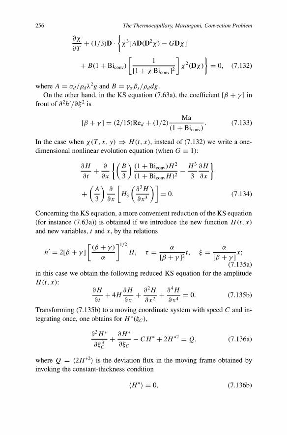
256 The Thermocapillary, Marangoni, Convection Problem
∂χ
∂T+ (1/3)D ·
{χ3[AD(D2χ) − GDχ]
+ B(1 + Biconv)
[1
[1 + χ Biconv]2
]χ2(Dχ)
}= 0, (7.132)
where A = σd/ρdλ2g and B = γσβs/ρddg.
On the other hand, in the KS equation (7.63a), the coefficient [β + γ ] infront of ∂2h′/∂ξ 2 is
[β + γ ] = (2/15)Red + (1/2)Ma
(1 + Biconv). (7.133)
In the case when χ(T , x, y) ⇒ H(t, x), instead of (7.132) we write a one-dimensional nonlinear evolution equation (when G ≡ 1):
∂H
∂t+ ∂
∂x
{(B
3
)(1 + Biconv)H
2
(1 + BiconvH)2− H 3
3
∂H
∂x
}
+(
A
3
)∂
∂x
[H3
(∂3H
∂x3
)]= 0. (7.134)
Concerning the KS equation, a more convenient reduction of the KS equation(for instance (7.63a)) is obtained if we introduce the new function H(t, x)
and new variables, t and x, by the relations
h′ = 2[β + γ ][(β + γ )
α
]1/2
H, τ = α
[β + γ ]2t, ξ = α
[β + γ ]x;(7.135a)
in this case we obtain the following reduced KS equation for the amplitudeH(t, x):
∂H
∂t+ 4H
∂H
∂x+ ∂2H
∂x2+ ∂4H
∂x4= 0. (7.135b)
Transforming (7.135b) to a moving coordinate system with speed C and in-tegrating once, one obtains for H ∗(ξC),
∂3H ∗
∂ξ 3C
+ ∂H ∗
∂ξC
− CH ∗ + 2H ∗2 = Q, (7.136a)
where Q = 〈2H ∗2〉 is the deviation flux in the moving frame obtained byinvoking the constant-thickness condition
〈H ∗〉 = 0, (7.136b)

Convection in Fluids 257
and 〈 〉 denotes averaging over one wavelength in the scaled moving, ξC –coordinate. If however, the constant-flux condition is imposed, Q = 0, equa-tion (7.136a) reduces to
∂3H ′
∂ξ 3C
+ ∂H ′
∂ξC− CH ′ + 2H ′2 = 0, (7.137)
and constraint (7.136b) is unnecessary and no longer holds, 〈H ′〉 �= 0.We observe that the constant-flux equation has one parameter less and in-
volves only one equation (7.137), whereas the two equations (7.136a, b) mustbe solved for the constant-thickness approach and two parameters Q and Care involved; for a detailed discussion of the properties of these equations(above, companion to KS), see [42]. There are myriad infinite wave families;in particular, we observe the solitary-wave regime and note that some fami-lies of waves are traveling-wave solutions which have unique solitary-waveshapes. It is important to note that after the solitary-wave regime, the wavebreaks into non-stationary, three-dimensional patterns. This implies that 3Dstationary waves either do not exist or have very short lifetimes, thus beinginsignificant. The final transition to interfacial ‘turbulence’ must then be an-alyzed with an entirely different approach. In Section 10.8 we return to thediscussion of solitary wave phenomena in a convection regime.
We observe that various authors (see, for instance, Parmentier et al. [43])were interested in a weakly nonlinear analysis of coupled surface-tension andgravitational-driven instability in a thin layer. Unfortunately, the existence ofsuch a coupled Bénard–Rayleigh–Marangoni model problem on the basis ofa rational analysis and asymptotic modelling was not demonstrated in thispublication. Yet, such an approach certainly deserves further investigation!Obviously when buoyancy is the single responsibility of convection, onlyrolls will be observed. As soon as capillary effects are present, the situationis more complex; however, a general tendency is observed and it appearsthat a hexagonal structure is preferred at the linear threshold. The more thethermocapillary forces are dominant with respect to the buoyancy forces, thelarger the size of the region where hexagons are stable. The influence of thePrandtl number has received particular attention from Parmentier et al. [43]!
Here it seems not superfluous to observe that the quantity βS (> 0) is de-fined as minus the vertical temperature gradient that would appear in a purelyconductive steady state (see, for instance, (1.19a, b)). Since in the pure heatconducting state, the temperature at the upper (flat) free surface is uniform,there is no ambiguity in determining experimentally βsd, which is related tothe difference between the temperature at the lower rigid plate (Tw) and thetemperature of the air surmounting the liquid layer (TA) (see (1.21b)), where
258 The Thermocapillary, Marangoni, Convection Problem
the Biot number (Bis) is defined with a constant heat transfer coefficientqs(Td), this assumption being strictly satisfied only when the temperature atthe upper free surface is uniform – such a condition is met in pure buoyancy-driven (RB) convection, i.e., when the upper free surface is rigid (a simpleRayleigh problem considered in Chapter 3); if we except the reference heatconductive steady case (1.19a), this is no longer true in Marangoni’s insta-bility (in BM thermocapillary convection) as the temperature at the upperdeformed (by the convection) free surface varies from point to point – theheat transfer coefficient qconv (or convection Biot number Biconv) is then nota constant! In a convection regime, when the fluid is set in motion, βS is nolonger the temperature gradient in the fluid layer since convection induces anon-zero mean perturbative temperature at the upper free fluid surface. Asa consequence the dimensionless numbers of Marangoni and Rayleigh mustbe experimentally evaluated with, as given by (1.21b),
βs = (Tw − TA)
[(k/qs) + d] , (7.138)
with k the thermal conductivity (assumed a constant) of the fluid layer.Namely (the subscript ‘0’ is relative to the ‘room’ temperature):
ρ ≈ ρ0[(T − T0)] with α0 = −(
1
ρ0
)[∂ρ
∂T
]0
,
σ (T ) ≈ σ0
[1 −
(γ0
σ0
)(T − T0)
]with γ0 = −
[∂σ (T )
∂T
]0
,
Ra = gα0βsd4
kν,
Ma = γ0βsd2
ρ0kν. (7.139)
In [43], as an alternative to the Marangoni (Ma) and Rayleigh (Ra) num-bers, Parmentier et al. define two new dimensionless numbers α and λ by therelations
αλ = Ra
Ra0and λ(1 − α) = Ma
Ma0, (7.140)
where Ra0 and Ma0 are two arbitrary constants – namely, Ra0 is the criticalRa for pure buoyancy and Ma0 is the critical Ma for pure thermocapillarity.According to Parmentier et al. [43], we observe that, in physical situations,the main control parameter is neither Ma nor Ra, but the temperature gradientβS defined above by (7.138). The use of α and λ is motivated by the fact

Convection in Fluids 259
that α is a combination of the relevant physical parameters, while λ is thequantity directly proportional to the control temperature difference. From(7.140), because
(1 − α)
[Ra
Ra0
]= α
[Ma
Ma0
], (7.141a)
we see that α can be considered as the percentage of buoyancy effect withregard to thermocapillary effect – it takes values between zero and one: α =0 corresponds to pure thermocapillarity and α = 1 to pure buoyancy. On theother hand, from the obvious relation
λ = Ra
Ra0+ Ma
Ma0, (7.141b)
we see that λ is directly proportional to the temperature gradient; in weaklynonlinear problems λ remains close to 1. A challenging problem, linked withthe above situation, is the formulation of a ‘correct’ dominant dimensionlessmodel, as this has been demonstrated here in Chapter 4 and the use, then, ofan IBL averaged approach! The analytical weakly nonlinear approach, givenin [43], via the derivation of a set of Ginzburg–Landau amplitude equationsand, then, to a consideration of a reduced system of three amplitude equa-tions, is interesting from a mathematical point of view (in particular, con-cerning the construction of a complete basis of eigenfunctions with the incor-poration a mode with a zero wave number in the nonlinear development) but,rather complicated to keep in mind the results obtained? Obviously the maininterest of the approach realized in [43] is the investigation related to thecompetition between hexagonal and roll patterns, which are the most currentpatterns observed near the threshold (the relative distance from the thresholdbeing given by ε = (λ−λc)/λc, with as critical lambda, λc = min(α,Bi, k),relative to the set ]0,∞[ of admissible values of the wave number k; the kcorresponding to λc is the critical k → kc. Except for pure buoyancy insta-bility, when α = 1, the convective patterns that appear at the linear thresholdare always formed with hexagons – below this threshold, a subcritical regionwhere hexagons can be stable is also found. Hexagonal patterns are unsta-ble when buoyancy is the only factor of instability. When the temperaturegradient is increased, a region where rolls and hexagons coexist is diplayed;at still higher temperature gradients, rolls are expected. We note that, whenbuoyancy is the single responsibility of the convection, only rolls will be ob-served. On the other hand, it appears that a hexagonal structure is preferredat the linear threshold. The more the thermocapillary forces are dominantwith respect to the buoyancy forces, the larger the size of the region wherehexagons are stable. The results of Parmentier et al. [43] very well exhibit

260 The Thermocapillary, Marangoni, Convection Problem
the fact that, by increasing temperature-dependent surface tension, one pro-motes the hexagonal pattern and, on the contrary, in the limiting case (in apure buoyancy thermal convection) of a negligible temperature dependenceof the surface tension, only rolls are stable. But it is necessary to note as wellthat the (in the thermocapillary case) important effect of a deformable freesurface is not taken into account in [43] and in, fact, the starting problem in[43] and in the Dauby and Lebon paper [44] are similar and are a consistentRB model problem which takes into account only partially the real effectlinked with the thermocapillarity (see our discussion in Section 5.2). Moreprecisely, the upper free surface condition for the dimensionless pressure πis not taken into account and just this condition poses a problem in a weaklyexpansible liquid subject to a temperature-dependent surface tension!
References
1. D.G. Crowdy, C.J. Lawrence and S.K. Wilson (Guest-Editors), The Dynamics of ThinLiquid Films. Special issue of J. Engng. Math. 50(2–3), 95–341, November 2004.
2. H.-C. Chang, Wave evolution on a falling film. Annu. Rev. Fluid Mech. 26, 103–136,1994.
3. P. Colinet, J.C. Legros and M.G. Velarde, Nonlinear Dynamics of Surface-Tension-Driven Instabilities, 1st Edn. Wiley-VCH, 2001.
4. A.A. Nepomnyaschy, M.G. Velarde and P. Colinet, Interfacial Phenomena and Convec-tion. Chapman & Hall/CRC, London, 2002.
5. M.G. Velarde and R.Kh. Zeytounian, Interfacial Phenomena and the Marangoni Effect.CISM Courses and Lectures, No. 428, CISM, Udine and Springer-Verlag, Wien/NewYork, 2002.
6. E. Guyon, J-P. Hulin and L. Petit, Hydrodynamique physique. Savoirs Actuels, InterEdi-tions/Editions du CNRS, Paris, Meudon, 1991.
7. E. Guyon, J-P. Hulin, L. Petit and C.D. Mitescu, Physical Hydrodynamics, Oxford Uni-versity Press, Oxford, 2001.
8. R.Kh. Zeytounian, The Bénard–Marangoni thermocapillary-instability problem. Phys.Uspekhi 41, 241–267, 1988.
9. C. Ruyer-Quil, B. Scheid, S. Kalliadasis, M.G. Velarde and R.Kh. Zeytouian, Thermo-capillary long waves in a liquid film fmow. Part 1. Low-dimensional formulation. J. FluidMech. 538, 199–222, 2005.
10. B. Scheid, C. Ruyer-Quil, S. Kalliadasis, M.G. Velarde and R.Kh. Zeytouian, Thermo-capillary long waves in a liquid film fmow. Part 2. Linear stability and nonlinear waves.J. Fluid Mech. 538, 223–244, 2005.
11. A. Oron, S.H. Davis and S.G. Bankoff, Long-scale evolution of thin liquid films. Rev.Modern Phys. 69(3), 931–980, 1997.
12. S.J. VanHook and J.B. Swift, Phys. Rev. E 56(4), 4897–4898, October 1997.13. M.F. Schatz, S.J. VanHook, W.D. McCormick, J.B. Swift and H.L. Swinney, Phys. Rev.
Lett. 75, 1938, 1995.14. D.J. Benney, Long waves on liquid films. J. Math. Phys. (N.Y.) 45, 150–155, 1966.
Convection in Fluids 261
15. P.M.J. Trevelyan and S. Kalliadasis, J. Engng. Math. 50(2-3), 177–208, 2004.16. C. Nakaya, Waves of a viscous fluid down a vertical wall. Phys. Fluids A1, 1143–1154,
1989.17. B. Sheid, A. Oron, P. Colinet, U. Thiele and J.C. Legros, Phys. Fluids 14, 4130–4151,
2002. Erratum: Phys. Fluids 15, 583, 2003.18. A. Pumir, P. Manneville and Y. Pomeau, J. Fluid Mech. 135, 27–50, 1983.19. P. Rosenau, A. Oron and J.M. Hyman, Phys. Fluids A4, 1102–1104, 1992.20. A. Oron and O. Gottlieb, Subcritical and supercritical bifurcations of the first- and-
second-order Benney equations. J. Engng. Math. 50(2–3), 121-140, 2004.21. S.-P. Lin, Finite amplitude side-band stability of a viscous film. J. Fluid Mech. 63, 417–
429, 1974.22. C. Ruyer-Quil and P. Manneville, Improved modeling of flows down inclined planes.
Eur. Phys. J. B15, 357–369, 2000.23. C. Ruyer-Quil and P. Manneville, Phys. Fluids 14, 170–183, 2002.24. V.Ya. Shkadov, Wave flow regimes of a thin layer of viscous fluid subject to gravity. Izv.
Akad. Nauk SSSR, Mekh. Zhidk. Gaza 2, 43–51, 1967 [English transl. in Fluid Dyn. 19,29–34, 1967.
25. R.Kh. Zeytounian, Long-Waves on Thin Viscous Liquid Film/Derivation of Model Equa-tions. Lecture Notes in Physics, Vol. 442, Springer-Verlag, Berlin/Heidelberg, pp. 153–162, 1995.
26. T. Ooshida, Phys. Fluids 11, 3247–3269, 1999.27. M.K.R. Panga and V. Balakotaiah, Phys. Rev. Lett. 90(15), 154501, 2003.28. C. Ruyer-Quil and P. Manneville, Phys. Rev. Lett. 93(19), 199401, 2004.29. S. Kalliadasis, A. Kiyashko and E.A. Demekhin, J. Fluid Mech. 475, 377–408, 2003.30. E.A. Demekhin, M. Kaplan and V.Ya Shkadov, Mathematical models of the theory of
viscous liquid films. Izv. Akad. Nauk SSSR, Mekh. Zhidk Gaza 6, 73–81, 1987.31. E.A. Demekhin and V.Ya Shkadov, Izv. Akad. Nauk SSSR, Mekh. Zhidk Gaza 5, 21–27,
1984.32. M. Takashima, J. Phys. Soc. Japan 50(8), 2745–2750 and 2751–2756, 1981.33. V.C. Regnier and G. Lebon, Q. J. Mech. Appl. Math. 48(1), 57–75, 1995.34. J.R.A. Pearson, On convection cells induced by surface tension. J. Fluid Mech. 4, 489–
500, 1958.35. D.A. Niels, Surface tension and buoyancy effects in cellular convection. J. Fluid Mech.
19, 341–352, 1964.36. P. Barthelet, F. Charry and J. Fabre, J. Fluid Mech. 303, 23, 1995.37. A.A. Golvin, A.A. Nepomnyaschy and L.M. Pismen, Phys. Fluids 6(1), 35–48, 1994.38. D. Kashdan et al., Nonlinear waves and turbulence in Marangoni convection. Phys. Flu-
ids 7(11), 2679–2685, 1995.39. A. Oron and Ph. Rosenau, Formation of patterns induced by thermocapillarity and grav-
ity. J. Phys. (France) II 2, 131–146, 1992.40. E. Erneux and S.H. Davis, Nonlinear rupture of free films. Phys. Fluids A5, 1117–1122,
1993.41. S.H. Davis, Annu. Rev. Fluid Mech. 19, 403–435, 1987.42. H.-C. Chang, E.A. Demekhin and D. Kopelevitch, Nonlinear evolution of waves on a
vertically falling fluid. J. Fluid Mech. 250, 433–480, 1993.43. P.M. Parmentier, V.C. Regnier and G. Lebon, Phys. Rev. E 54(1), 411–423, 1996.44. P.C. Dauby and G. Lebon, J. Fluid Mech. 329, 25–64, 1996.

Chapter 8Summing Up the Three Significant ModelsRelated with the Bénard Convection Problem
8.1 Introduction
One year ago, in reply to my proposal concerning the ‘possible’ publica-tion of the present book, with a clear emphasis on rational analysis and as-ymptotic modelling in derivation of model equations for the main kinds ofconvective flows, Professor René Moreau, Series Editor of FMIA, wrote tome:
. . . However, from a certain point of view, you know that some readersdo not care much for this rigor and just want to know what are therelevant model equations for their problem . . .
and later:
May I ask you a question? Could you imagine to add, in a kind ofgeneral conclusion, a sort of table made on the following idea, which,in my opinion, would significantly increase the potential sales.
This short chapter, with a summing up of Chapters 3, and 5 to 7, is, to acertain extent, a reponse to the above suggestion from Professor Moreau.Nevertheless, I hope that the preceding seven chapters have captured the in-terest of the majority of my readers and that, for them, this chapter will serveas only a concentrated review, at least concerning the sections devoted to RB,deep and BM convections. In the preceding chapters, our main objective wasa rational clarification of the various steps which lead to now well-knownapproximate leading-order, Rayleigh–Bénard (shallow-thermal), Zeytounian(deep-thermal) and Bénard–Marangoni (thermocapillarity-surface tension)convections. As a starting physical phenomemon we chose the simplest Bé-nard problem of a liquid layer heated from below, in the absence of rotation,
263

264 Three Significant Models Related with the Bénard Convection Problem
magnetic field, porous-medium or two-component fluid (for definitions ofsuch convections, see Chapter 10).
In a horizontal liquid layer, an adverse temperature gradient (βS) is main-tained by heating the underside (a lower horizontal rigid, z = 0, heated planeat temperature, Tw). The occurence of the phenomena seems to be associatedwith cooling of the liquid at its deformable (free at the reference, conduction,level z = d) surface (where exposed to the air, at temperature TA), when thelayer of the liquid is at a temperature somewhat above that assumed by a thinsuperficial film.
A very slight excess of temperature in the layer of the liquid above that ofthe surrounding air is sufficient to institute the ‘tesselated’ changing structure(according to Thompson [1], as this was noted by Lord Rayleigh in 1916).More precisely, the conduction adverse temperature gradient in liquid, βS ,is directly determined by the difference of temperature (Tw − TA), via aNewton’s cooling law of heat transfer with a unit constant thermal surfaceconductance qs :
βs = (Tw − TA)
[(k/qs) + d]where k is the thermal conductivity of the liquid and d the thickness of thelayer, both constant in a conduction motionless state.
In the simplest Bénard problem of a liquid layer heated from below, withβS , we have four main driving effects:
1. the buoyancy directly related to the thermal shallow convection,2. the temperature-dependent surface tension which is responsible for the
thermocapillary convection,3. the viscous dissipation which leads to consideration to deep thermal
convection, and4. the effect related to the influence of the deformable free surface.
These four effects affect mainly the Bénard convection phenomenon andit is necessary from the start of formulation of the full Bénard problem totake into account these four driving forces. In Figure 8.1 we have sketched(with pecked lines) the significant interconnections between these three mainfacets of Bénard convection.

Convection in Fluids 265
Fig. 8.1 Three main facets of Bénard convection.
8.2 A Rational Approach to the Rayleigh–Bénard ThermalShallow Convection Problem
In Chapter 3, in the framework of the simple Rayleigh thermal convectionproblem, the reader was initiated into our rational analysis and asymptoticmodelling approach. The keys to such an approach are based, from the begin-ning, on consideration of a problem formulation with the four main driving
266 Three Significant Models Related with the Bénard Convection Problem
forces, mentioned above, and careful analysis of the influence of the variousparameters which govern these driving forces! In the case of the classicalBénard, heated from below, thermal convection, the main driving force (inparticular when, as in Chapter 3, the liquid layer is between two rigid hor-izontal planes) is the buoyancy, and the Grashof, Gr, number (or Rayleigh,Ra, number) governs the RB shallow thermal convction, when we assumethat the liquid is weakly expansible.
We first define the expansibility parameter by
ε = α(Td)�T, (8.1a)
where, with ρ = ρ(T ), the influence of the pressure being negligible at theleading order,
α(Td) = −(
1
ρd
)[dρ(T )
dT
]d
and �T = Tw − Td (8.1b)
with Tw, the temperature at the lower horizontal rigid plane (z = 0) and Td ,the temperature at the upper horizontal rigid plane or the reference level ofthe deformable free surface (z = d). Then, the square of the Froude numberrelative to the constant conduction thickness d of the liquid layer (where νdis the kinematic viscosity, at temperature Td) being
Fr2d = (νd/d)
2
gd, (8.1c)
we discovered that the usual Grashof Gr number is simply the ratio of ε toFr2
d!
Gr = ε
Fr2d
= g
[−dρ(T )
dT
]d
(Tw − Td)d3
ρdν2d
. (8.1d)
The definition of the Grashof number as the ratio of the small expansibilityparameter (ε) to the square of the Froude number (Fr2
d), is the first main keystep to a rational derivation of the RB model problem. On the other hand,when the Prandtl number (at T = Td)
Pr = νd
κd= O(1) (8.1e)
is not very low or very large (νd ≈ κd where κd is the thermal diffusivity)the Rayleigh number
Ra ≡ Pr Gr = g
[−dρ(T )
dT
]d
(Tw − Td)d3
ρdνdκd
Convection in Fluids 267
plays a similar role as Gr; but both cases, when Pr � 1 or Pr � 1, deserveparticular attention (see some references in Chapter 10).
The second key step in rational, asymptotic derivation of the RB equa-tions for the shallow thermal convection, emerging from Tw > Td or moreprecisely, from
�T
d= βs
(≡ −dTs(z)
dz
)> 0, (8.2a)
where Ts(z) = Tw − βsz, is the conduction temperature in a steady motion-less state, is related to the introduction of a dimensionless temperature for aconvection regime:
θ = (T − Td)
dβs, (8.2b)
and its companion dimensionless pressure
π =(
1
Fr2d
){[(p − pd)
gdρd
]+ z − 1
}. (8.2c)
With ρ = ρ(T ) we write, according to (8.2a, b),
ρ = ρ(T = Td +�T θ) ≈ ρd(1 − εθ), (8.2d)
with an error of O(ε2).In a third key step, when the limiting (à la Boussinesq) process
ε → 0 and Fr2d → 0, simultaneously ≡ lim
Boussinesq(8.3a)
is performed, such that
Gr = ε
Fr2d
= O(1) is fixed, (8.3b)
from the dimensionless starting full Navier–Stokes and Fourier equations foran expansible liquid we derive, first, as continuity equation, the divergence-free constraint
∇ · u = εdθ
dt⇒ ∇uRB = 0, (8.3c)
for the limiting value of the dimensionless velocity
uRB = limBoussinesq
u.
On the other hand, from the dimensionless momentum equation for u, as aconsequence of the Boussinesq limiting process (8.3a), when we take into

268 Three Significant Models Related with the Bénard Convection Problem
account (8.2b–d), the following limit leading-order equation for the aboveuRB is derived:
duRB
dt+ ∇πRB − Gr θRBk = �uRB, (8.3d)
which is asymptotically correct in the leading order, with an error of O(ε).Now, it is necessary (as a fourth key step) to derive also a limit equation
forθRB = lim
Boussinesqθ
and for this from the starting energy equation (for the specific internal energy,e) it is necessary to first obtain the corresponding equation for the temper-ature; in the case of the simple equation of state ρ = ρ(T ) this is an easyexercise, because in such a case e = E(T ) and
dE
dt=
(dE
)dT
dt, (8.4a)
where dE/ = C(T ) is the specific heat for our expansible liquid.Nevertheless, an essential problem is elucidation of the role of the viscous
dissipation term in the dimensionless equation for temperature T . This vis-cous dissipation term, in a non-dimensional equation for the temperature T ,is proportional to dissipation parameter Di, such that
(1/2 Gr)Di ≡ (1/2 Gr)ε Bo, (8.4b)
where the so-called ‘Boussinesq number’ is given by
Bo = gd
C(Td)�T. (8.4c)
Gr is O(1) and fixed when we perform the above Boussinesq limiting process(8.3a). From (8.4b) we see that:
if Bo = O(1) fixed, when (8.3a) is realized, then Di → 0.
In such a case, for the above dimensionless temperature θRB, we obtain fromthe full equation for the dimensionless temperature θ , defined by (8.2b), themodel, leading-order equation
dθRB
dt=
(1
Pr
)�θRB. (8.4d)
The condition Bo = O(1) gives the following constraint for the thickness d:
dT
dT

Convection in Fluids 269
d ≈ C(Td)�T
g,
and we obtain that the limiting, leading-order, shallow RB convection equa-tions (8.3c, d) and (8.4d), for uRB, πRB and θRB, are valid in a liquid layerthickness d such that
1 mm ≈(ν2d
g
)1/3
� d ≈ C(Td)�T
g. (8.5)
For the à la Rayleigh model problem considered above, the boundary con-ditions are very simple because the convection operates (as a direct conse-quence of a low squared Froude number Fr2
d � 1) inside a constant horizon-tal incompressible liquid layer, z ∈ [0, 1], and in such a case,
uRB = 0 and θRB = 1 on z = 0; uRB = 0 and θRB = 0 on z = 1.(8.6)
When, as in Chapter 5, we assume that above the liquid layer exists an am-bient atmosphere (passive air) and, as a consequence, it is necessary to takeinto account, in the starting formulation of the Bénard convection problem,heated from below, the presence of a deformable free surface, obviously theabove conditions on z = 1 must be replaced by more complicated upper con-ditions! But, curiously, in the framework of the limiting process (8.3a), andin particular because Fr2
d → 0, these conditions are considerably simplified.The reason being that, for the dimensionless pressure π , defined by (8.2c),the associated dimensionless upper condition is written rigorously as:
π = [H(t, x1, x2)− 1]Fr2
d
+(∂u′
i
∂x′j
+ ∂u′j
∂x′i
)n′in
′j
+ (We − Maθ)(∇‖ · n)− (2/3)εdθ
dt,
on z = H [= 1 + ηh(t, x, y)], (8.7a)
and we observe that We and Ma are defined in Chapter 1 by (1.18a, b).Fr2
d → 0 being the denominator, we can only assume that H → 1 – asa consequence, in a rational theory it is necessary to assume the followingsimilarity rule (assuming that the dimensionless deformation of the upperfree surface h = O(1)) between two small parameters η and Fr2
d :
η
Fr2d
= η∗ = O(1) when Fr2d → 0 and η → 0 simultaneously. (8.7b)

270 Three Significant Models Related with the Bénard Convection Problem
From (8.7b) for the RB model system of shallow convection the upper, free-surface condition must be written (at least to leading order) on z = 1.
According to results of Section 5.2, we obtain, on z = 1,
uRB · k ≡ u3RB = 0, (8.7c)
∂2u3RB
∂z2= Ma
[∂2θRB
∂x2+ ∂2θRB
∂y2
], (8.7d)
∂θRB
∂z+ [1 + BiconvθRB] = 0. (8.7e)
Finally, from (8.7a) we derive with (8.7b), when we assume that We � 1and
η We = We∗ = O(1), (8.8a)
an equation for the free-surface deformation h(t, x, y),
∂2h
∂x2+ ∂2h
∂y2−
(η∗
We∗
)h = −
(1
We∗
)π(t, x, y, z = 1). (8.8b)
The reader has now, in the above few pages, all information linked tothe full theoretical statement of the shallow Rayleigh–Bénard convectionleading-order model problem. Further, if the reader wants to obtain thesecond-order model equations (with non-Boussinesq effects) associated withthe leading-order shallow RB model equations, then this is an easy task as isshown in Sections 3.5 and 3.6 and also in Section 5.3.
In fact, 25 years ago, in October 1983, I first published a short note [1] inComptes Rendus de l’Académie des Sciences – Paris entitled ‘One Asymp-totic Formulation of Rayleigh–Bénard’s Problem via Boussinesq Approxi-mation for the Expansible Liquid’.
A recent book by Getling [2] gives a pertinent account linked with the‘structure and dynamics’ of the Rayleigh–Bénard convection. In a more re-cent review paper, by Bodensghatz et al. [3], the reader can find a modern ac-count relative to theoretical and experimental investigations of the Rayleigh–Bénard convection problem. Finally, we observe that equation (8.8b) for thefree-surface deformation h(t, x, y) has been first derived thanks to our ratio-nal analysis and asymptotic modelling!
8.3 The Deep Thermal Convection with Viscous Dissipation
An attentive examination of the dominant equation for the dimensionlesstemperature θ shows that, as a consequence of the à la Boussinesq, lim-
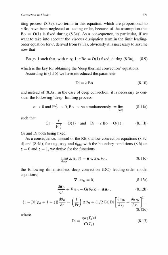
Convection in Fluids 271
iting process (8.3a), two terms in this equation, which are proportional toε Bo, have been neglected at leading order, because of the assumption thatBo = O(1) is fixed during (8.3a)! As a consequence, in particular, if wewant to take into account the viscous dissipation term in the limit leading-order equation for θ , derived from (8.3a), obviously it is necessary to assumenow that
Bo � 1 such that, with ε � 1: ε Bo = O(1) fixed, during (8.3a), (8.9)
which is the key for obtaining the ‘deep thermal convection’ equations.According to (1.15) we have introduced the parameter
Di = ε Bo (8.10)
and instead of (8.3a), in the case of deep convection, it is necessary to con-sider the following ‘deep’ limiting process:
ε → 0 and Fr2d → 0, Bo → ∞ simultaneously ≡ lim
deep(8.11a)
such thatGr = ε
Fr2d
= O(1) and Di = ε Bo = O(1), (8.11b)
Gr and Di both being fixed.As a consequence, instead of the RB shallow convection equations (8.3c,
d) and (8.4d), for uRB, πRB and θRB, with the boundary conditions (8.6) onz = 0 and z = 1, we derive for the functions
limdeep
(u, π, θ) = uD, πD, θD, (8.11c)
the following dimensionless deep convection (DC) leading-order modelequations:
∇ · uD = 0, (8.12a)
duD
dt+ ∇πD − Gr θDk = �uD, (8.12b)
{1 − Di[pd + 1 − z]}dθD
dt=
(1
Pr
)�θD + (1/2 Gr)Di
[∂uDi
∂xj
+ ∂uDj
∂xi
]2
,
(8.12c)where
Di = gα(Td)d
C(Td)(8.13)

272 Three Significant Models Related with the Bénard Convection Problem
is our ‘depth’ parameter, defined in 1989 in [4] by δ. For the DC equations(8.12a–c) as boundary conditions, we have again
uD = 0 and θD = 1 on z = 0; uD = 0 and θD = 0 on z = 1. (8.14)
But we can also consider these DC equations (8.12a–c) with the ‘upper, non-deformable (on z = 1), free-surface’ conditions, as in (8.12c–e) with (8.8a,b). I think that these DC equations with viscous dissipation term deservevarious complementary investigations linked with a more detailed accountof modifications introduced to the classical Rayleigh–Bénard shallow con-vection structure, dynamics and attractors via the route to chaos.
8.4 The Thermocapillary Convection withTemperature-Dependent Surface Tension
If we want to consider the full effect of a temperature-dependent tension onthe upper, deformable free-surface conditions, then it is imperative to assumethat the square of the Froude number Fr2
d is fixed and of order 1 when theexpansibility parameter ε tends to zero. In such a case, at leading order, theeffect of buoyancy is negligible and the limit (relative to ε → 0) modelequations are simply the usual Navier incompressible equations for
limε→0
(u, π) = (uBM, πBM) (8.15a)
and the à la Fourier usual temperature equation for
limε→0
= θBM, (8.15b)
namely,∇ · uBM = 0, (8.16a)
duBM
dt+ ∇πBM = �uBM, (8.16b)
PrdθBM
dt= ��BM. (8.16c)
However, in the framework of the Bénard-Marangoni (BM) model prob-lem, for the model equations (8.16a–c), we have complicated upper, de-formable free-surface conditions, because the similarity rule (8.7b) is unnec-essary when Fr2
d = O(1). Namely, we write on the upper-deformable freesurface, z = H(t, x, y):
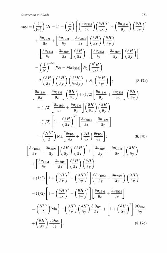
Convection in Fluids 273
πBM =(
1
Fr2d
)(H − 1)+
(2
N
){(∂u1BM
∂x
)(∂H
∂x
)2
+(∂u2BM
∂y
) (∂H
∂y
)2
+ ∂u3BM
∂z+
[∂u1BM
∂y+ ∂u2BM
∂x
](∂H
∂x
)(∂H
∂y
)
−[∂u1BM
∂z+ ∂u3BM
∂x
] (∂H
∂x
)−
[∂u2BM
∂z+ ∂u3BM
∂y
] (∂H
∂y
)}
−(
1
N
)3/2
[We − Ma θBM]{N2
(∂2H
∂x2
)
− 2
(∂H
∂x
)(∂H
∂y
)(∂2H
∂x∂y
)+N1
(∂2H
∂y2
)}; (8.17a)
[∂u1BM
∂x− ∂u3BM
∂z
] (∂H
∂x
)+ (1/2)
[∂u1BM
∂y+ ∂u2BM
∂x
] (∂H
∂y
)
+ (1/2)
[∂u2BM
∂z+ ∂u3BM
∂y
] (∂H
∂x
)(∂H
∂y
)
− (1/2)
[1 −
(∂H
∂x
)2] [
∂u3BM
∂x+ ∂u1BM
∂z
]
=(N1/2
2
)Ma
[∂θBM
∂x+
(∂H
∂x
)∂θBM
∂z
]; (8.17b)
[∂u1BM
∂x− ∂u2BM
∂y
] (∂H
∂y
) (∂H
∂x
)2
+[∂u2BM
∂y− ∂u3BM
∂z
](∂H
∂y
)
+[∂u1BM
∂z+ ∂u3BM
∂x
] (∂H
∂x
) (∂H
∂y
)
+ (1/2)
[1 +
(∂H
∂x
)2
−(∂H
∂y
)2](
∂u1BM
∂y+ ∂u2BM
∂x
) (∂H
∂x
)
− (1/2)
[1 −
(∂H
∂x
)2
−(∂H
∂y
)2][
∂u2BM
∂z+ ∂u3BM
∂y
]
=(N1/2
2
)Ma
{−
(∂H
∂x
)(∂H
∂y
)∂�BM
∂x+
[1 +
(∂H
∂x
)2]∂�BM
∂y
+(∂H
∂y
)∂�BM
∂z
}. (8.17c)

274 Three Significant Models Related with the Bénard Convection Problem
Next, for θBM as upper free-surface condition we have
∂θBM
∂z+N1/2(1 + BiconvθBM) = ∂θBM
∂x
(∂H
∂x
)+ ∂θBM
∂y
(∂H
∂y
), (8.17d)
while the kinematic condition is unchanged:
u3BM = ∂H
∂t+ u1BM
(∂H
∂x
)+ u2BM
(∂H
∂y
). (8.17e)
The full BM model problem for the phenomena of thermocapillarity isvery complicated and necessitates a numerical computation, but this BMmodel problem is relative to thin films (of the order of the millimetre) andwhen the amplitude of the free surface deformation is moderate we havethe possibility to consider, instead of the above BM problem (8.16a–c),(8.17a–e), a BM reduced long-wave model problem which has been dis-cussed in Section 7.3, see (7.29a–d). Such a computation for the thermo-capillary waves has been proposed recently, in [5, 6]. This computation hasbeen described in [6] with the help of a regularized reduced model derivedin [5]; see also Section 10.4.
In recent years, several books have been published relative to thermocap-illary temperature-dependent, surface tension driven, Marangoni convectionby Colinet et al. [7], Velarde and Zeytounian [8], and Nepomnyaschy et al.[9].
Obviously the present book, mainly devoted to an analytical approach tothe full Bénard problem, heated from below, and its rational analysis and as-ymptotic modelling, have really, relative to purpose, very little overlap withthe above cited books! Our fundamental concept is the possibility to ex-tract, consistently, from this very complicated, but ‘rich’ Bénard, physical-mathematical problem, three relatively simple but significant approximatemodel problems.
On the other hand, to those familiar with the large panoply of films, liquidlayers, and their behavior in its full complexity and variety, the approach andthe derived model problems in this present book may seem abstract and re-mote. Nonetheless, I consider the field to have come a long way; at least nowwe are, from the start of formulation of the problem, devoted to modellingthe main physical driving effects, whereas two decades ago a large numberof papers were based on ad hoc pseudo-theoretical approaches and numeri-cal computations. In the meantime, I hope that careful study of these sevenpreceding chapters in this volume will kindle new insights into the Bénardproblem, and perhaps suggest fresh approaches.

Convection in Fluids 275
References
1. R.Kh. Zeytounian, Sur une formulation asymptotique du problème de Rayleigh–Bénard,via l’approximation de Boussinesq pour les liqudes dilatables. C. R. Acad. Sci., Paris Ser.I 297, 271–274, October 1983.
2. A.V. Getling, Rayleigh–Bénard Convection: Structure and Dynamics. World Scientific,Singapore, 1998.
3. E. Bodenschatz, W. Pesch and G. Ahlers, Ann. Rev. Fluid Mech. 32, 709–778, 2000.4. R.Kh. Zeytounian, The Bénard problem for deep convection: Rigorous derivation of ap-
proximate equations. Int. J. Engng. Sci. 27(11), 1361–1366, 1989.5. C. Ruyer-Quil, B. Scheid, S. Kalliadasis, M.G. Velarde and R.Kh. Zeytounian, Thermo-
capillary long-waves in a liquid film flow. Part 1. Low-dimensional formulation, J. FluidMech. 538, 199–222, 2005.
6. B. Scheid, C. Ruyer-Quil, S. Kalliadasis, M.G. Velarde and R.Kh. Zeytounian, Thermo-capillary long-waves in a liquid film flow. Part 2. Linear stability and nonlinear waves, J.Fluid Mech. 538, 223–244, 2005.
7. P. Colinet, J. Legros and M.G. Velarde, Nonlinear Dynamics of Surface-Tension-Driven-Instabilities, 1st Edn. Wiley/VCH, 2001.
8. M.G. Velarde and R.Kh. Zeytounian, Interfacial Phenomena and the Marangoni Effect,1st Edn. CISM Courses and Lectures, No. 428, Udine, Springer-Verlag, Wien/New York,2002.
9. A.A. Nepomnyaschy, M.G. Velarde and P. Colinet, Interfacial Phenomena and Convec-tion. Chapman & Hall/CRC, London, 2002.

Chapter 9Some Atmospheric Thermal ConvectionProblems
9.1 Introduction
The thermal convection problems considered in this chapter are very dif-ferent from the scales in time and space of the phenomena studied in thepreceding chapters. As this is well and pertinently discussed in the paper byVelarde and Normand [1], published in July 1980 in Scientific American:
In the Earth’s atmosphere convection is observed at several scales oflength. The temperature gradient between the Tropics and the polesdrives a global circulation, which can be decomposed into at least threelarge convective cells in each hemisphere. Distortions of these patternscaused by the rotation of the Earth give rise to the trade winds of theTropics and the prevailing westerlies of the temperate zones.
Local heating of the atmosphere near the Earth’s surface gives riseto smaller-scale convective flows, including those of most storms. Cu-mulus clouds, which form when warm air rises and cools and therebybecomes supersaturated with moisture, often mark the convective over-turning of the atmosphere.
A theoretical analysis of atmospheric convection must take into ac-count the compressibility of air, which gives rise to a density gradienteven when the temperature is constant with height.
An accurate description of atmospheric circulation would also haveto include the compressive heating of air when it sinks into a regionof higher pressure. Viscosity and other properties of air also vary withpressure and temperature, and the presence of water vapor, which givesup heat when it condenses, adds still another level of complexity!
277

278 Some Atmospheric Thermal Convection Problems
It is obvious that the theories that describe these convective processes requiremany simplifying assumptions, if they are to be of any practical use, Eventhen they are far from simple! But, it is therefore all the more remarkable thatthese few related theories, governed by a handful of dimensionless numbers,can account for phenomena that differ so greatly in scale.
It is interesting to note that Prandtl, in 1944, obtained an explicit solutionof a local very simple thermal convection model problem on the assumptionthat the idealized mountain slope under consideration consists of an infinite,thermally homogeneous plane. Namely (see, for instance, chapter 7 in thebook by Gutman [2]), in such a simple case, the thermal convection phe-nomenon is governed by the following two linear equations, for the tempera-ture perturbation θ , and horizontal velocity u along the mountain slope withinclination angle α with respect to the horizontal direction:
∂θ
∂t+ Su sin α = k
∂2θ
∂z2, (9.1a)
∂u
∂t− λθ sinα = ν
∂2u
∂z2. (9.1b)
When the stratification parameter S and parameter of convection λ are bothconstant, with k ≡ ν = const, the steady-state solution of equations (9.1a,b), satisfying the conditions
z = 0: u = 0, θ = θ0 = const and u → 0, θ → 0 when z → ∞,
(9.1c)is of the following form (when S > 0):
u = θ0
[(λ
S
)]1/2
exp(−ξ) sin ξ and θ = θ0 exp(−ξ) cos ξ, (9.2a)
where
ξ = z[(λS) sin2 α
4ν2
]1/4. (9.2b)
For the neutral or unstable stratification (S ≤ 0) of the undisturbed at-mosphere, equations (9.1a, b) do not have steady-state solutions which wouldsatisfy conditions (9.1c). Obviously, the solution (9.2a) can be used as a testfor convergence and for the accuracy of the more realistic numerical solu-tion. In Section 9.5, the reader can find some complements which generalizethe above simple Prandtl example.
Our intention in this chapter is not to give a full account of the variousconvective atmospheric phenomena (for this even a volume would not suf-fice), but rather to illustrate via some typical problems the rich variety of
Convection in Fluids 279
these convective atmospheric phenomena. The reader can find in the bookby Emanuel [3] a relatively recent text devoted entirely to ‘atmospheric con-vection’.
Concerning the Boussinesq approximation and the associated Boussinesqatmospheric equations which are a very good approximation for the slow(hyposonic, [4]) atmospheric motions, the reader can find in [5], and in themore recent paper [6] various information relative to the rational derivationof these Boussinesq atmospheric equations for dry air assumed to be a ther-mally perfect gas.
Namely, in this chapter I study only some particular (mainly meso or lo-cal) convection motions in the atmosphere. After this introduction, in Sec-tion 9.2, the formulation of the breeze problem via the Boussinesq hydro-static approximation is considered and Section 9.3 is then devoted to the in-fuence of a local temperature field in an atmospheric Ekman layer via a tripledeck asymptotic approach. In Section 9.4, a periodic, double-boundary layerthermal convection over a curvilinear wall is investigated. In Section 9.5,some other particular atmospheric convection problems are also briefly dis-cussed.
9.2 The Formulation of the Breeze Problem via the BoussinesqHydrostatic Approximation
We consider a first local atmospheric convection phenomenon, the freecirculation-breeze problem. The modeling of this breeze problem is directlyrelated to the justification of the Boussinesq hydrostatic approximation foratmospheric convection and, for this, it is necessary to start from the full,non-adiabatic and non-hydrostatic, viscous, unsteady, and compressible NSFequations and take into account a rotating system of spherical coordinates.
In a coordinate frame rotating with the Earth, we consider from the be-ginning the full NSF equations (for a thermally perfect gas) and take intoaccount, first, the Coriolis force (2� ∧ u), the gravitational acceleration(modified by the centrifugal force) g, and also the effect of thermal radiationQ. The (relative) velocity vector is u = (v, w), as observed in the Earth’sframe rotating with the angular velocity �. The thermodynamic functionsare again, ρ (atmospheric air density), p (atmospheric air pressure) and T
(absolute temperature of dry thermally perfect air).First, we assume that

280 Some Atmospheric Thermal Convection Problems
dRs
dzs= ρsQ with Rs = Rs(Ts(zs)), (9.3a)
and we note that ρs(zs) and Ts(zs), in relation (9.3a), are the density andtemperature in the hydrostatic reference state (function only of the altitude zsin the reference state). The heat source Q (i.e., thermal radiation) is assumedto be only a function of this hydrostatic reference state via the ‘standard’temperature Ts(zs). Doing this, we consider only a so-called, mean, standard,distribution for Q and ignore variations from it for the perturbed atmospherein motion (namely, in a ‘convection’ regime). The temperature Ts(zs), for thehydrostatic reference state (in a so-called ‘standard atmosphere’), satisfiesthe following (balance) equation, written here in dimensional form:
kcdTsdzs
+ Rs(Ts(zs)) = 0, (9.3b)
where the conductivity kc = const (in a simplified case). Now � can beexpressed as
� = �0e with e = k sin ϕ + j cos ϕ, (9.4)
where �0 = const and ϕ is the algebraic latitude of the point P 0 of the ob-servation on the Earth’s surface, around which the atmospheric convections(free circulations) are analyzed (in the Northern Hemisphere, ϕ > 0). Theunit vectors directed to the east, north, and zenith (in the opposite directionfrom g = −gk), are denoted by i, j, and k, respectively. It is helpful to em-ploy spherical coordinates λ, ϕ, r, and in this case u, v, w denote again thecorresponding relative velocity components in these directions, respectively,increasing azimuth (λ), latitude (ϕ), and radius (r). However, it is very con-venient to introduce here the transformation
x = a0 cos ϕ◦, y = a0(ϕ − ϕ◦), z = r − a0, (9.5)
where ϕ◦ is a reference latitude (for ϕ◦ ≈ 45◦ we have a0 ≈ 6367 km,which is the mean radius of the Earth), and the origin of this right-handedcurvilinear coordinates system lies on the Earth’s surface (for a flat ground,where r = a0) at latitude ϕ◦ and longitude λ = 0.
We assume therefore that the atmospheric convection phenomenon occursin a midlatitude, mesoscale region, distant from the equator (sin ϕ◦, cos ϕ◦,and tan ϕ◦ are all of order unity), and in this case the sphericity parameter
δ = L0
a0is assumed small. (9.6)

Convection in Fluids 281
Although x and y are, in principle, new longitude and latitude coordinates interms of which the NSF atmospheric equations may be rewritten without ap-proximation (see, for instance, [5, chapter II]), they are obviously introducedin the expectation that (for small δ, in the leading order, with a sufficientlygood approximation) will be the Cartesian coordinates of the so-called f ◦-plane (tangent) approximation.
In fact, in the breeze problem, it is necessary to take into account the influ-ence of the Coriolis force as a main driving force, and also write a boundarycondition for the temperature expressing the influence of a local thermal non-homogeneity on flat ground surface; such a condition has, for example, thefollowing form:
T = Ts(0) + (�T )0� at z = 0, (9.7)
with � is a given (known data) function of the time and the position on abounded region D (of diameter L0) on the flat ground surface. As a conse-quence, we have the possibility to introduce a vertical characteristic lengthscale (R is the perfect gas constant)
h0 = R(�T )0
g� L0, (9.8a)
such that
τ = (�T )0
Ts(0)≡ gh0
RTs(0)� 1. (9.8b)
On the one hand, the height h0 = 103 m is significant for the breeze phenom-enon and, on the other hand, when we take into account the Coriolis force inthe dynamic atmospheric unsteady viscous equation, the horizontal charac-teristic length scale L0 for this breeze phenomenon is L0 ≈ 105 m and as aconsequence the Rossby number
Ro = U0
f ◦L0≈ 1 with f ◦ = 2�0 sin ϕ◦, (9.8c)
where U0 can be evaluated after a judicious choice when we consider thebreeze as a low Mach number,
M = U0
[γRTs(0)]1/2� 1, (9.8d)
phenomenon, such that (γ = ratio of the specific heats)
τ
M= τ ∗ ≈ 1 ⇒ U0 ≈ (�T )0
[γR
Ts(0)
]1/2
. (9.8e)

282 Some Atmospheric Thermal Convection Problems
Obviously, as long-wave parameter we must now consider the ratio
λ = h0
L0� 1, (9.9a)
and for a high Reynolds number
Re = U0L0
ν0� 1, (9.9b)
where the kinematic viscosity ν0 is assumed constant, the following hydro-static limit process must be performed:
λ → 0 and Re → ∞, simultaneously, such that λ2Re = Re⊥ = O(1).(9.9c)
We observe that, when we use (9.8a), (9.8e), and (9.9a, b), with (9.9c) we de-rive the following value for the temperature rate (�T )0, in thermal boundarycondition (9.7):
(�T )0 ≈(R
g
)2/3 (1
ν0L0
)1/3 [γR
Ts(0)
]1/6
. (9.9d)
When dimensionless time-space variables are considered,
t ′ = t
(1/�0), x′ = x
L0, y′ = y
L0and z′ = z
h0(9.10a)
then, for the dimensionless horizontal velocity vector v′, vertical velocity w′,pressure p′, density ρ ′, and temperature T ′, we write:
v′ = U0v, w′ = λU0w, p′ = ps(0)p, ρ ′ = ρs(0)ρ, T ′ = Ts(0)T ,(9.10b)
where v′, w′, p′, ρ ′, and T ′ are dependent on t ′, x′, y′, and z′.Finally, with the Stokes relation, under the hydrostatic limit process (9.9c)
we derive the following set of dimensionless quasi-hydrostatic dissipative(Q-HD) equations for vQ−HD, wQ−HD, pQ−HD, ρQ−HD, and TQ−HD:
SdρQ−HD
dt ′+ ρQ−HD
[D′ · vQ−HD + ∂wQ−HD
∂z′
]= 0; (9.11a)
ρQ−HD[S dvQ−HD
dt ′+
(1
Ro
)(k ∧ vQ−HD)+
(τ
γM2
)D′pQ−HD
=(
1
Re⊥
)∂2vQ−HD
∂z′2 ; (9.11b)

Convection in Fluids 283
∂pQ−HD
∂z′ + τρQ−HD = 0; (9.11c)
ρQ−HDSdTQ−HD
dt ′−
[(γ − 1)
γ
]S
dpQ−HD
dt ′
=(
1
Pr Re⊥
) [∂2TQ−HD
∂z′2 + (γ − 1)PrM2
∣∣∣∣∂vQ−HD
∂z′
∣∣∣∣2
+ τ 2�0dR′
S(T′S(z
′S))
dz′S
]; (9.11d)
pQ−HD = ρQ−HDTQ−HD. (9.11e)
In the quasi-hydrostatic dissipative equations (9.11a–e) we have
Sd
dt ′= S
∂
∂t ′+ vQ−HD · D′ + wQ−HD
∂
∂z′ ,
where S = L0�0/U0 is the Strouhal number, Pr = Cpµ0/k0 the usual
Prandtl number (with Cp the specific heat at pressure constant and µ0 =ρs(0)ν0, the constant dynamic viscosity) and D′ = (∂/∂x′, ∂/∂y′), k·D′ = 0.In equation (9.11d) for TQ−HD the dimensionless parameter �0 is a measurefor the (standard) heat source term. We observe that, if we assume that theStrouhal number S ≈ 1, then the characteristic time is such that
Ro = 1
(2 sin ϕ◦)≈ 1, (9.12)
and in such a case, unsteadiness and the Coriolis force are both operative inequation (9.11b) for the horizontal velocity vector in the convection problem– but in equation (9.11b) we have the small Mach number M. In standardatmosphere, from equation (9.11d), in particular we obtain for T ′
S(z′S) (the
dimensionless temperature in hydrostatic reference state), with the relation:
z′S = τz′, (9.13)
(because z′ = z/h0 but z′S = zS/HS , with HS = RTs(0)/g) according to
(9.8b) the following dimensionless equation for TS(z′S), instead of (9.3b).
dTS(z′S)
dz′S
+�0R′S(T
′S(z
′S)) = 0. (9.14)
In fact, (9.14) is an equation defining T ′S(z
′Z) via R′
S(T′S(z
′S)), when the judi-
cious boundary conditions are assumed in z′S . This determination of T ′
S(z′S)

284 Some Atmospheric Thermal Convection Problems
is in reality a complicated problem; see, for instance, Kibel’s book [7, sec-tion 1.4] – but, for our purpose here this problem has no influence, becausez′S tends to zero with τ tending to zero (when z′ is fixed, see (9.13)), andT ′S(0) ≡ 1.
For equations (9.11a–e), from (9.7) in dimensionless form we write asthermal boundary condition at the flat ground:
TQ−HD = 1 + τ�(t ′, x′, y′), (9.15)
for (x′, y′) ∈ D and T ′ ≡ 1, if (x′, y′) �∈ D. Now, from the Q-HD equations(9.11a–e), with (9.15), we can derive via a Boussinesq limit:
τ → 0 and M → 0 withτ
M= τ ∗ ≈ 1, (9.16)
with the following ‘low Mach number asymptotics’:
vQ−HD = vconv + O(M), w = wconv + O(M),
pQ−HD = p′S(z
′S)[1 +M2πconv + · · ·],
TQ−HD = T ′S(z
′S)[1 +Mθconv + · · ·],
ρQ−HD = ρ ′S(z
′S)[1 +Mωconv + · · ·], (9.17)
a set of hydrostatic viscous, non-adiabatic Boussinesq-convective equations,for the functions vconv, wconv, πconv, θconv, and ωconv. Namely (dropping theprime ′), these Boussinesq Hydrostatic-Convection (BH-C) equations (à laZeytounian) are written in the following form:
D · vconv + ∂wconv
∂z= 0; (9.18a)
Sdvconv
dt+
(1
Ro
)(k ∧ vconv)+
(1
γ
)Dπconv = Gr−1/2
⊥∂2vconv
∂z2; (9.18b)
∂πconv
∂z+ τ ∗θconv = 0; (9.18c)
Sdθconv
dt+ τ ∗�(0)wconv =
(1
Pr
)Gr−1/2
⊥∂2θconv
∂z2; (9.18d)
ωconv = −θconv, (9.18e)
where
Sd
dt= S
∂
∂t+ vconv · D + wconv
∂
∂z. (9.19a)

Convection in Fluids 285
In equation (9.18d), as stratification parameter, we have
�(0) =[(γ − 1)
γ
]+
[dTS(zS)
dzS
]0
, (9.19b)
and instead of 1/Re⊥ we have introduced the Grashof number defined by
Gr⊥(≡ Re2⊥) ≡ λ2 Gr with Gr = γ R
[h0(�T )0/ν0]2
TS(0). (9.19c)
Indeed, the model equations (9.18a–e), with (9.19a–c), for the freecirculation-convection breeze phenomena, can be considered as an inner(significant, boundary layer) degeneracy of full atmospheric NSF equations,when two limit processes, (9.9c) and (9.16), with (9.17), are performed. But,because the corresponding outer degeneracy gives the trivial zero solution(as a consequence of the local character of the free circulation-convectionphenomenon), we can write the behavior of the free circulation far (whenz ↑ ∞, there is no outer solution) from the assumed flat ground surfacez = 0. Namely, for model equations (9.18a–e), the following boundary con-ditions (see (9.7) with (9.17) and (9.16)) are obtained:
z ↑ ∞: (vconv, wconv, πconv, θconv) → 0; (9.20a)
z = 0: vconv = wconv = 0, (9.20b)
z = 0: θconv = τ ∗(t, x, y) when (x, y) ∈ D, (9.20c)
z = 0: (vconv, wconv, πconv, θconv) ≡ 0, (x, y) �∈ D. (9.20d)
We observe that the breeze is a localized (regional) phenomenon and, in fact,it is active mainly on the bounded region D at the Earth’s surface.
Concerning the initial conditions at t = 0, for vconv and θconv, it is neces-sary to consider an unsteady adjustment problem if we want to study the ini-tial, near t = 0, strongly unsteady transition, short-time scale phenomenon– as in [8], particular attention must be given to short-time-scale unsteadysolutions near t = 0 (see, for instance Section 10.8). But here we have, infact, two unsteady adjustment, short-time scale, problems!
We observe also that the order of equations (9.18a–e), with respect to z,does not allow us (because we have the reduced equation (9.18c) insteadof a full unsteady equation for w) to specify a behavior condition for wconv
when z → +∞! But, in particular, from equation (9.18d) for θconv, when�(0) �= 0, since θconv → 0 when z → +∞, we should also have
wconv = 0 at z = ∞; (9.21)

286 Some Atmospheric Thermal Convection Problems
this constraint (9.21), not being a boundary condition, should be satisfiedautomatically. On the other hand, from (9.18a) with conditions (9.20a, b) wederive also a second constraint:
D ·∫ ∞
0vconv = 0. (9.22)
Consequently, the presence in equation (9.18d) for θconv of the term τ ∗�(0),which in general is not small compared with the other terms in (9.18d), leadsin a stably stratified standard atmosphere to the formation of a percepti-ble compensating flow (anti-breeze) which exists above the main breeze, aphenomenon well-known from observations in nature (see, for example, thebook by Khrgian [9]).
From the BH-C system of equations (9.18a–e) we can derive two simpli-fied systems for the breeze phenomena, and the reader can verify the accu-racy of both these simplified model equations.
First, in the two-dimensional case (vconv ≡ ui, ∂/∂y = 0), when the effectof the rotation is not taken into account and in boundary condition (9.20c) onz = 0 for the function �, we have the following simple form (when t > 0),
� = [α + βx] sin t, (9.23a)
where α and β are two specified constants. Quantity β can be interpreted assome characteristic gradient of the underlying-surface temperature, α beinga maximum difference between the temperature of land and sea, divided bythe characteristic length of the phenomenon. This simplified form (9.23a) issatisfied best in some sufficiently small region (and in this case the Coriolisforce is not active) in the vicinity of the shore line, to the order of a fewkilometers in both directions.
Using (9.23a), the 2D solution with above assumed simplifications issought in the form
u = u(t, z), θconv = ϑ(t, z)+xσ (t, z),(
1
γ
)πconv = ϕ(t, z)+xψ(t, z),
(9.23b)and in such a case,
D · vconv ≡ 0, wconv = 0, (9.23c)
because wconv = 0 at z = 0. Substitution of (9.23b, c) in (9.18b–d) yields asimplified system in which the functions are not a function of x:
S∂u
∂t+ ψ =
(1√Gr⊥
)∂2u
∂z2; (9.24a)

Convection in Fluids 287
S∂ϑ
∂t+ uσ =
(1√Gr⊥
)∂2ϑ
∂z2; (9.24b)
S∂σ
∂t=
(1√Gr⊥
)∂2σ
∂z2; (9.24c)
∂ϕ
∂z=
(τ ∗
γ
)ϑ; (9.24d)
∂ψ
∂z=
(τ ∗
γ
)σ. (9.24e)
The system of equations (9.24a–e) should be solved subject to the followingboundary conditions:
u = 0, ϑ = τ ∗α sin t, σ = τ ∗β sin t for z = 0; (9.25a)
u = 0, ϑ = 0, σ = 0, ϕ = 0, ψ = 0 for z = ∞. (9.25b)
It is clear that the system of equations (9.24a–e) represents a chain of inter-actions between various physical effects operating in the breeze mechanism,namely:
(9.24c) ⇒ (9.24e) ⇒ (9.24a) ⇒ (9.24d)⇓ ⇑(9.24b)
First, from equation (9.24c), for σ , it follows that the horizontal temperaturegradient is produced in the atmosphere due to heating of air by conduction ofheat from the underlying surface. Then, equation (9.24e) shows that the ap-pearance of this horizontal temperature gradient leads to the appearance of ahorizontal pressure gradient. Later, equation (9.24a) indicates that the pres-sure gradient induces the onset of (breeze) wind; here an important role isplayed by eddy diffusion. Further, equation (9.24b) demonstrates the oppo-site effect, exerted by the wind on the temperature field, where the nonlinearterm uσ represents a negative heat source in the heat conduction equation(9.24b), and it is precisely this term which describes the wind transport ofheat. Finally from (9.24d), a main pressure field ϕ is induced via the tem-perature field, in particular, the solution for ϕ, via (9.24d), gives the dailypressure variation at the underlying-surface level (z = 0).
Solutions of the above set of equations show that the structure of thisbreeze model in vicinity of the shore (the x-axis is directed normal to theshore and the coordinate origin (x = y = 0) is taken at the shore line onthe asumption of a straight and infinite shore, the y-axis being along the

288 Some Atmospheric Thermal Convection Problems
shore) is similar to the wind and temperature progressive wave damping outwith altitude. It is important that from this model we established the instantwhen the wind appears at the ground on the onset of breeze – at this instant,∂u/∂z|z=0 – and thus it is found that the breeze lags behind the variation inthe soil temperature by six hours (this is a rough result, since the observationsyield from two to five hours). More important, this model points out the causeof this lag, which is inertia moving air.
A second simplified model is linked with a local wind arising above aslope (as in Prandtl’s 1944 example, mentioned above) the steepness ofwhich is not less than several degrees and the deviation of the surface tem-perature of which, from the temperature of the free atmosphere at the samealtitude, exceeds in absolute value several degrees centigrades and changeslittle along the slope; this is a so-called ‘slope wind’ on the assumption thatit develops in an atmosphere at rest.
Our purpose below is to derive (in a rational way) a specific system ofmodel equations for this slope wind, from the equations (9.18a–e); for thispurpose, the first problem is the introduction of the topography in equations(9.18a–e)?.
The slope is assumed to be given by the equations
z =( |F |
h0
)F(x, y) with |F | = max(F ), when (x, y) ∈ D, (9.26a)
where h0 is given by (9.8a).From Cartesian coordinates (x, y, z) we pass to curvilinear coordinates
(ξ, η, ζ ) by
ξ = x, η = y, ζ = z − F0F(ξ, η), F0 ≡( |F |
h0
), (9.26b)
and we write∂
∂z= ∂
∂ζ; (9.27a)
∂
∂x= ∂
∂ξ− F0
(∂F
∂ξ
)∂
∂ζ; (9.27b)
∂
∂y= ∂
∂η− F0
(∂F
∂η
)∂
∂ζ; (9.27c)
D · vconv + ∂wconv
∂z= ∂usl
∂ξ+ ∂vsl
∂η+ ∂ωsl
∂ζ; (9.27d)

Convection in Fluids 289
Sd
dt= S
∂
∂t+ vsl · D + ∂ωsl
∂ζ, (9.27e)
where
ωsl = wsl − F0
[(∂F
∂ξ
)usl +
(∂F
∂η
)vsl
]= wsl − F0(vsl · DF), (9.27f)
D =(∂
∂ξ,∂
∂η
)and vsl = (usl, vsl). (9.27g)
Then elementary transformations yield, instead of the system of equations(9.18a–d), the following equations for usl, vsl, ωsl, πsl, and θsl, which arefunctions of the time t , and curvilinear coordinates, ξ , η, ζ :
D · vsl + ∂ωsl
∂ζ= 0; (9.28a)
Sdvsl
dt+
(1
Ro
)(k ∧ vsl) +
(1
γ
)Dπsl −
(F0
γ
)τ ∗DFθsl
= Gr−1/2⊥
∂2vsl
∂ζ 2; (9.28b)
∂πsl
∂ζ+ τ ∗θsl = 0; (9.28c)
Sdθsl
dt+ τ ∗�(0)[ωsl + F0(vsl · DF)] =
(1
Pr
)Gr−1/2
⊥∂2θsl
∂z2. (9.28d)
The boundary conditions associated with (9.28a–d) are
ζ = 0: vsl = 0; ωsl = 0;θsl = τ ∗�(t, ξ, η), and for t > 0, (ξ, η) ∈ D, (9.29a)
ζ → ∞: |ξ 2 + η2| → ∞; vsl → 0; πsl → 0;θsl → 0 ⇒ ωsl → 0. (9.29b)
However, in the case of the slope wind we see that
1√Gr⊥
� 1, (9.30a)
and the following (outer) limit process is considered below:

290 Some Atmospheric Thermal Convection Problems
1√Gr⊥
→ 0 with t, ξ, η, ζ fixed. (9.30b)
With (9.30a, b), we obtain only a trivial zero outer solution
voutsl = 0, πout
sl = 0, θoutsl = 0, ωout
sl = 0. (9.31)
As a consequence, it is necessary to derive associated inner equations, viathe introduction of an inner vertical coordinate and an inner vertical velocity
ζ ∗ = ζ
[Gr]−1/4and ω∗
sl = ωsl
[Gr]−1/4, (9.32a)
and consider an inner limit process
1√Gr⊥
→ 0 with t, ξ, η, ζ ∗ fixed. (9.32b)
As a result of (9.32a, b) we derive for the limit values v∗sl, ω∗
sl, π∗sl, θ∗
sl, asfunction of t , ξ , η and ζ ∗, the following system of model boundary layerequations which governs the slope wind local phenomenon:
D · v∗sl +
∂ω∗sl
∂ζ ∗ = 0; (9.33a)
Sdv∗
sl
dt+
(1
Ro
)(k ∧ v∗
sl) +(
1
γ
)Dπsl −
(F0
γ
)τ ∗DFθ∗
sl
= ∂2v∗sl
∂ζ ∗2; (9.33b)
∂π∗sl
∂ζ ∗ = 0; (9.33c)
Sdθ∗
sl
dt+ τ ∗(0)F0(vsl · DF) =
(1
Pr
)∂2θ∗
sl
∂ζ ∗2. (9.33d)
But from (9.33c), as in classical boundary layer theory,
π∗sl ≡ π∗
sl(t, ξ, η) = πoutsl
∣∣ζ=0 = 0, (9.34a)
and from (9.30a),
1√Gr⊥
� 1 ⇒(
h0
L0
)2
Re = h20U0
ν0L0 1,
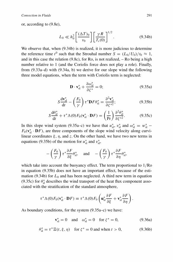
Convection in Fluids 291
or, according to (9.8e),
L0 � h20
[(�T )0
ν0
] [γ R
Ts(0)
]1/2
. (9.34b)
We observe that, when (9.34b) is realized, it is more judicious to determinethe reference time t0 such that the Strouhal number S = (L0/U0)/t0 ≈ 1,and in this case the relation (9.8c), for Ro, is not realized, – Ro being a highnumber relative to 1 (and the Coriolis force does not play a role). Finally,from (9.33a–d) with (9.34a, b) we derive for our slope wind the followingthree model equations, when the term with Coriolis term is neglected:
D · v∗sl +
∂ω∗sl
∂ζ ∗ = 0; (9.35a)
Sdv∗
sl
dt−
(F0
γ
)τ ∗DFθ∗
sl = ∂2v∗sl
∂ζ ∗2; (9.35b)
Sdθ∗
sl
dt+ τ ∗(0)F0(v∗
sl · DF) =(
1
Pr
)∂2θ∗
sl
∂ζ ∗2. (9.35c)
In this slope wind system (9.35a–c) we have that u∗sl, v∗
sl and ω∗sl = w∗
sl −F0(v∗
sl · DF), are three components of the slope wind velocity along curvi-linear coordinates ξ , η, and z. On the other hand, we have two new terms inequations (9.35b) of the motion for u∗
sl and v∗sl,
−(
F0
γ
)τ ∗ ∂F
∂ξθ∗
sl, and −(
F0
γ
)τ ∗ ∂F
∂ηθ∗
sl,
which take into account the buoyancy effect. The term proportional to 1/Roin equation (9.35b) does not have an important effect, because of the esti-mation (9.34b) for L0 and has been neglected. A third new term in equation(9.35c) for θ∗
sl describes the wind transport of the heat flux component asso-ciated with the stratification of the standard atmosphere,
τ ∗(0)F0(v∗sl · DF) ≡ τ ∗(0)F0
(u∗
sl∂F
∂ξ+ v∗
sl∂F
∂η
).
As boundary conditions, for the system (9.35a–c) we have:
v∗sl = 0 and ω∗
sl = 0 for ζ ∗ = 0, (9.36a)
θ∗sl = τ ∗�(t, ξ, η) for ζ ∗ = 0 and when t > 0, (9.36b)

292 Some Atmospheric Thermal Convection Problems
v∗sl, ω∗
sl, θ∗sl → 0 for |ξ 2 + η2| → ∞, (9.36c)
v∗sl,
∂ω∗sl
∂ζ ∗ , θ∗sl → 0 for ζ ∗ → ∞. (9.36d)
The Prandtl example, (9.1a, b) with (9.1c), is a simplified case of the derivedmodel (9.35a–c) with (9.36b–d).
9.3 Model Problem for the Local Thermal Prediction – A TripleDeck Viewpoint
Below we consider only a two-dimensional steady local thermal problem andrewrite the thermal boundary condition (9.7) in the following form:
T
Ts(0)= 1 + τ�
( xl0
)on z = 0, (9.37)
where � ≡ 0 when |x/l0| ≤ 1, where l0 is the local horizontal length scale.Far upstream, when x → −∞ and � ≡ 0, we assume that we have a basicundisturbed flow which is characterized by an Ekman layer profile:
UEk
(x
L0,(z/ l0)
κ0
)= UG
(x
L0
){1 − exp
[−(z/ l0)
κ0
]cos
[−(z/ l0)
κ0
]},
(9.38a)where
κ0 = [�0 sin ϕ0/ν0]−1/2
l0≡
[Rel
2Rol
]−1/2
, (9.38b)
with4
4 When the ‘global’ Rossby number is formed via L0, RoL = (U0/L0)/2�0 sinϕ0, thenin basic atmospheric flow, undisturbed by the local thermal condition (9.37), we assume thatRoL � 1 and because the Mach number M is also small in equation (9.11b), we consider thedouble limit process
RoL → 0 and M → 0, such that RoL/γM = Go = O(1) and Re⊥ = O(1).
As a result we obtain at the leading order (outer limit), when S, Go, τ∗, t , x, y, z are fixed,the so-called ‘geostrophic relation’. For instance, when in equation (9.11a), Re⊥ = O(1) andS = O(1) are both fixed, we have [5]:
k ∧ vG+ τ∗ Go DpG = 0. (*)
The above geostrophic relation (*) is strongly singular near the initial time, t = 0, and inthe vicinity of the ground, z = 0. In the vicinity of z = 0, when we assume that in (9.11a)Re⊥ � 1 such that

Convection in Fluids 293
Rel = U0l0
ν0and Rol = (U0/ l
0)
2�0 sin ϕ0, (9.38c)
the local Reynolds and Rossby numbers, based on the local horizontal lengthscale l0.
If in the local thermal problem we non-dimensionalize the horizontal andvertical coordinates with l0: x′ = x/l0 and z′ = z/ l0, then in the dimension-less local problem appears, also, a local Boussinesq number
Bol = gl0
RTs(0). (9.38d)
If l0 ≈ 103 m, then Bol � 1 and in such a case, Rel � 2Rol � 1. Therefore,in this case we can assume
2Rol = (Rel)−1/a ⇒ κ0 = (Rel)
−1/m, (9.39a)
with (0 < a < 1) and
m = (2 − a)
(1 − a)> 2. (9.39b)
For example, if U0 ≈ 10 m/sec, ν0 ≈ 5 m2/sec and f 0 ≡ 2�0 sin ϕ0 ≈10−4 1/sec, the considered case, l0 ≈ 103 m, leads to m = 5. For this case,we have the possibility to use as
l0 ≈(U0
g
)[RTs(0)
γ
]1/2
⇒ BolM
= B∗ ≡ 1, (9.39c)
and the Boussinesq approximation is correct.
RoL/Re⊥ ≡ Ek⊥ = E∗ Ro2L
with E∗ = O(1), (**)
then, instead of the geostrophic relation (*), when (inner limit): RoL → 0, with E∗, Go, t , x,y, and inner vertical coordinate, z/Ro = z∗ fixed, we derive the equation
k ∧ vG + τ∗ Go DpG = E∗ ∂2vG∂z∗2
. (***)
Via matching between outer and inner limits, we then have the possibility, with (*) and(***), to derive the so-called Ackerblom’s model problem, and obtain the Ekman layer profile(9.37). In [5, chapter vii, §28], the reader can find a consistent asymptotic derivation of thisAckerblom’s model problem, which allows us to derive a boundary condition on the ground,taking into account the influence of the Ekman layer, on the main quasi-geostrophic equationfor pG, in (*).
In geostrophic wind UG(x/L0), L0 is a ‘global’ horizontal length scale and this ‘global’horizontal length scale is also present in the Ekman layer UEk profile (9.38a).

294 Some Atmospheric Thermal Convection Problems
The value m = 5 is the same as the one used by Smith and coworkers [10,11] for the flow over an isolated two-dimensional short hump in the boundarylayer. In [12], the Boussinesq stratified fluid flow is also considered.
When m = 5 we have that a typical triple deck case exist:
l0
L0≈ Re−3/8
L where ReL = L0U0
ν0. (9.39d)
(in [13, pp. 211–220], the reader can find a more general approach). Now,according to the Boussinesq approximation, taking into account (9.39b), wehave the possibility to formulate the following dimensionless local steadythermal problem (where the main small parameter is κ5
0 and defined by(9.39a):
u∂u
∂x+ w
∂u
∂z+
(1
γ
)∂π
∂x= κ5
0
(∂2u
∂x+ ∂2u
∂z2
), (9.40a)
u∂w
∂x+ w
∂w
∂z+
(1
γ
)∂π
∂z−
(1
γ
)B∗θ = κ5
0
(∂2w
∂x+ ∂2w
∂z2
), (9.40b)
∂u
∂x+ ∂w
∂z= 0, (9.40c)
u∂θ
∂x+ w
∂θ
∂z+ B∗�(0)w =
(1
Pr
)κ5
0
(∂2θ
∂x+ ∂2
∂z2
), (9.40d)
ω = −θ, (9.40e)
when we assume, as in (9.16), that (see also (9.8e))
τ → 0, M → 0 andτ
M= τ ∗ ≈ 1. (9.41)
As boundary conditions we write:
z = 0: u = w = 0, θ = τ ∗(x), 0 ≤ x ≤ 1, (9.42a)
and also, according to our formulation of the considered interaction problembetween the local thermal spot and Ekman atmospheric layer,
x → −∞: u → 1−exp
[− z
κ0
]cos
[− z
κ0
]≡ U∞
(z
κ0
), w, π, θ → 0,
(9.42b)and we note that:
ifz
κ0→ ∞, then u → 1, for x → −∞ (9.42c)

Convection in Fluids 295
ifz
κ0→ 0, then u ≈ z
κ0, for x → −∞. (9.42d)
Now, if we need to take into account the boundary conditions on theground z = 0, then it is necessary to introduce an inner coordinate
z∗ = z
κα0
, α > 1, and in this case u ≈ κα−10 z∗ for x → −∞. (9.43a)
From equation (9.40a) for u we verify that, if u ≈ κα−10 u∗(x, z∗), then for the
consistency (κα−10 u∗∂u∗/∂z∗ + · · · = κ5−2α
0 ∂2u∗/∂z∗2 + · · ·), it is necessaryto assume that
α − 1 = 5 − 2α ⇒ α = 2. (9.43b)
Finally, it is clear that three vertical coordinates (z) are necessary for theasymptotic triple deck analysis (when κ0 → 0) of the system (9.40a–e).Namely:
(a) z, for an ‘upper non-viscous region’, where
u ≈ uup → 1 when x → −∞, (9.44a)
(b) ζ = z/κ0, for a ‘middle, intermediate, region’, where
u ≈ um → 1 − eζ cos ζ ≡ U∞(ζ ) when x → −∞, (9.44b)
(c) z∗ = z/κ20 , for a ‘lower, wall, viscous region’, where
u ≈ κ0u∗ and u∗ → z∗ when x → −∞. (9.44c)
For the other case, when l0/L0 < Re−3/8L or l0/L0 > Re−3/8
L , it is necessaryto apply a different asymptotic analysis (see, for example, the approach bySmith et al. in [14]). But the case m = 6 and m = 4 can be analyzed fromthe system (9.40a–e). For the case m = 3 it is necessary to start from anotherproblem, where the Boussinesq approximation does not emerge – in this casewe have l0 ≈ 104 m and we may neglect again the Coriolis terms in the local,but non-Boussinesq, equations!
Concerning the analysis of the so-called ‘triple-deck’ structure, the readercan find in [15, chapter 12], a detailed account of this triple deck approach,when a singular – different from the classical à la Prandtl – direct couplingbetween boundary layer and non-viscous fluid flow, coupling of a three lay-ered structure is necessary!
Below, we give only the main result of this triple deck analysis. Namely,in wall, viscous, lower region, where the significant vertical coordinate is z∗

296 Some Atmospheric Thermal Convection Problems
we derive, instead of equations (9.40a–e), for the function u∗, v∗, and θ∗, thefollowing leading-order system:
u∗ ∂u∗
∂x+ w∗ ∂w
∗
∂z∗ +(
1
γ
)B∗
∫ z∗
∞
(∂θ
∂x
)dz∗
+(
1
γ
)dP(x)
dx= ∂2u∗
∂z∗2; (9.45a)
∂u∗
∂x+ ∂w∗
∂z∗ = 0; (9.45b)
u∗ ∂θ∗
∂x+ w∗ ∂θ
∗
∂z∗ =(
1
Pr
)∂2θ∗
∂z∗2, (9.45c)
with
z∗ = 0: u∗ = w∗ = 0, θ∗ = τ ∗�(x), 0 ≤ x ≤ 1, (9.46a)
z∗ → ∞: u∗ → z∗, w∗ → 0, θ∗ → 0,
P (x) → 0, A(x) → 0,dA
dx→ 0, (9.46b)
x → −∞: u∗ → z∗ + A(x), w∗ → −z∗ dA
dx, θ∗ → 0, (9.46c)
after matching with the middle deck (region via ζ → 0 ⇔ z∗ → ∞). To beprecise, in the middle deck as solution we have
um = A(x)dU∞(ζ )
dζand wm = −
(dA(x)
dx
)U∞(ζ ), (9.47)
which represents simply a vertical displacement of the streamline through adistance −κ0A(x), the function A(x) being related to the pressure πup in theupper deck by
[∂2
∂x2+ ∂2
∂z2+K2
0
]∂πup
∂x= 0, K2
0 =(B∗2
g
)�(0), (9.48a)
with at z = 0:
∂
∂x
[∂πup
∂z
]= γ
[K2
0
dA(x)
dx+ d3A(x)
dx3
]. (9.48b)
On the other hand, the flow in the upper deck is driven by an outflow fromthe middle deck, and far from the above solution (9.47), for wm, we have

Convection in Fluids 297
limζ→∞wm(x, ζ ) = −dA
dx. (9.49)
In the middle deck we have also
U∞(ζ ) ≈ ζ anddU∞(ζ )
dζ≈ 1 when ζ → 0. (9.50)
Finally, in the lower deck, associated with the problem (9.45a–c), (9.46a–c),we have the following relation between π∗ and θ∗:
∂π∗
∂z∗ = B∗θ∗ ⇒ π∗ = B∗∫ z∗
∞θ∗ dz∗ + P(x). (9.51)
The specification of the model problem (9.45a–c), (9.46a–c), with (9.49),(9.50) and (9.51), is completed by the relations (9.48a, b) between P(x) andA(x), since
πup(x, 0) ≡ P(x). (9.52)
The well-known interpretation of (9.52) is that the pressure P(x) drivingthe flow in the lower deck is itself induced in the main (upper) stream, i.e.,the upper deck, by the displacement thickness of the lower deck transmittedthrough the middle deck by the passive effect of displacement of the stream-lines. The strong singular self-induced coupling arises because the problem(9.45a–c), (9.46a–c) to be solved in the lower viscous deck (layer) does notaccept P(x) as data known prior to the resolution, as is the case in the frame-work of the classical Prandtl boundary layer problem. On the contrary, thispressure perturbation P(x) must be calculated at the same time as the ve-locity components u∗ and w∗, as well as the temperature perturbation θ∗.Nevertheless, it must be emphasized that P(x) is related to A(x)! This rela-tion is explicit in the linear case, when the parameter τ ∗, in condition (9.46a)for θ∗, is considered as a small parameter. We observe also that via a Fouriertransform
Fk(f (x)) ⇒ f F (k),
instead of (9.48b) we obtain the following relation between AF (k) andPF (k):
AF (k) =[iN0
γ
] [PF (k)
(K20 − k2)
], (9.53a)
where
N0 = i[k2 −K20 ]1/2 if |k| > K0 and [K2
0 − k2]1/2 if |k| < K0.(9.53b)
Here we have applied (in the upper region) the standard radiation conditionfor z → ∞, choosing the sign of N for |k| < K0, so that the wave modescarry energy only upwards.

298 Some Atmospheric Thermal Convection Problems
9.4 Free Convection over a Curved Surface – A SingularProblem
Below, a simplified case considered by Schlichting [16] in 1932 has beengeneralized to a periodic nonlinear free convection over a curvilinear surface.This study leads to the conclusion that, in the case of small surface slope, theconvection flow above the surface exhibits a special structure; steady sec-ondary flows are generated above the surface, throughout the region wherethe convection takes place. Moreover, it appears that these secondary flowsdo not depend on viscosity and thermal conductivity. Rather they create asupplementary temperature perturbation on the curved surface and a veloc-ity field far from this surrface.
These results were obtained in 1961 in Moscow Meteo-Center (during myresearch in I. A. Kibel’s Dynamic Meteorology Department) and publishedonly in 1968 [17]. For a two-dimensional case the dimensionless startingequations are a particular case of the model equations (9.33a–d), with
Ro = ∞, S = Pr = 1 and �(0) = 0, (9.54)
and in such a case we write for the dimensionless velocity componentsu(t, s, n) and w(t, s, n), and perturbation of the temperature θ(t, s, n), thefollowing equations:
∂u
∂t+ β
[u∂u
∂s+ w
∂u
∂n
]= �θ + ∂2u
∂n2, (9.55a)
∂u
∂s+ ∂w
∂n= 0, (9.55b)
∂θ
∂t+ β
[u∂θ
∂s+ w
∂θ
∂n
]= ∂2θ
∂n2, (9.55c)
where β is a small parameter which is a measure of the effect of the nonlinearterms and also the supplementary surface perturbation temperature, θ andvelocity component u far from the curved surface. The boundary conditionsfor the system (9.55a–c) are
n = 0: u = w = 0, θ = cos t + βA(s), (9.56a)
n → ∞: u → βB(s), θ → 0. (9.56b)
If now we introduce the stream function ψ(t, s, n) and write
ψ = ψ0 + βψ1 + · · · , θ = θ0 + βθ1 + · · · , (9.57)

Convection in Fluids 299
then as first approximation we obtain
ψ0 = (1/2)�
{sin
(π
4− t
)−
(1√2
)e−n/
√2
[cos
(n√2
− t
)
+(
1 + n√2
)sin
(n√2
− t
)]}; (9.58a)
θ0 = e−n/√
2
[cos
(n√2
− t
)]. (9.58b)
Concerning the second approximation ψ1 and θ1, we can write
ψ1 = �d�
ds[ψ1pe2it + ψ1 st], θ1 = d�
ds[θ1pe2it + θ1 st], (9.59)
where the subscript ‘p’ is relative to the periodic part and subscript ‘st’ tothe steady-state part.
Here we write only the formula for ψ1 st and θ1 st. Namely:
θ1 st = −(1/4)e−n/√
2 sinn√2
− (1/8√
2)(2√
2 + n)e−√2n + C1n + C2;
(9.60a)
ψ1 st = −(1/8√
2)
{(1/2)e−√
2n
[n2 +
(9√2
)n + (25/2)
]
+ 2e−n/√
2
[(2 + n√
2
)cos
n√2
− 2 sinn√2
]
− C3n2 + C4n + C5; (9.60b)
From the boundary conditions we obtain
C1 = C2 = 0 and C3 = 0, C4 = −7/8, C5 = 41
32√
2; (9.60c)
A(s) = −(1/4)d�
ds, B(s) = −(7/8)�
d�
ds. (9.60d)
Figure 9.1 is the result of a computation, with the help of the derivedformula, of the variation in perturbation of the temperature with altitude n forvarious time t . The dashed line represent the linear case (first approximation)and we see that nonlinear terms change strongly the vertical structure of theperturbed temperature.
Obviously our above approach is based on a particular ‘strategy’ whichallows us to avoid the necessity of introducing an outer representation of

300 Some Atmospheric Thermal Convection Problems
Fig. 9.1 Vertical structure of θ for various time values. Reprinted with kind permission from[17].
the approximate solution far from the heated surface! In Figure 9.1 the po-sition s on the heated curved surface is s = 0.3 and the function �(s) =[3(3/2)1/2]s(1 − s2). For simplicity of computation, we choose β = 1!The supplementary perturbations are positives on the heated curved surfacewhen �(s) decreases and negatives when �(s) increases. Concerning thesecondary current, far from a heated curved surface, it is directed in the di-rection where the function �(s) decreases.
In fact, an associated representation near the heated surface is unneces-sary. This was shown by Noe in his thesis [18]. Noe considered, for thefar region, an outer representation and by matching obtained a uniformlyvalid approximate solution above the heated surface. In his asymptotic the-ory (1981) Noe shows the non-existence of a proximate layer near the curvedheated surface and as a consequence the singular behavior of θ and ψ is re-lated only, for both fields, to n tending to infinity – far from the heated curvedsurface.
Obviously the first approximation (9.58a, b) is uniformly valid. Far fromthe heated curved surface, Noe assumed that the far region, when n → ∞,is characterized by
n = βγ n∗ with γ < 0, (9.61a)

Convection in Fluids 301
and wrote
ψ − (1/2)�
{[(1 + i)
2√
2
]eit +
[(1 − i)
2√
2
]e−it
}= βϕψ∗(t, s, n∗;β),
(9.61b)θ = βσ θ∗(t, s, n∗;β). (9.61c)
The analysis and matching, between outer (far region) and near (wherethe classical solution remains valid) regions, give
s = 1, 1 + ϕ − γ = −2γ and ϕ = 3γ ⇒ ϕ = −3/4, γ = −1/4.(9.61d)
We observe that Noe’s approach is consistent only when in equation(9.55c), for θ , the stratification term is absent! Curiously, the choice C1 = 0,in our solution (9.60a), according to Noe’s analysis, is correct and confirmsthe analysis performed by Riley in 1965 [19] for the case of ‘oscillating vis-cous flows’. In [13, chapter xi], the reader can find a detailed account of theso-called ‘double boundary layer model’ of Riley [19] and Stuart [20], rel-ative to the ‘high frequency oscillating viscous flow, large Strouhal number,case’.
Finally, for the steady-state dominant problem in the far/outer region, Noeobtained the following coupled problem for ψ∗
st and θ∗st:(
∂ψ∗st
∂n∗
)∂2ψ∗
st
∂s∂n∗ −(∂ψ∗
st
∂s
)∂2ψ∗
st
∂n∗2
= �(s)θ∗st + ∂3ψ∗
st
∂n∗3, (9.62a)
(∂ψ∗
st
∂n∗
)∂θ∗
st
∂s−
(∂ψ∗
st
∂s
)∂θ∗
st
∂n∗ = ∂2θ∗st
∂n∗2, (9.62b)
with, as boundary conditions,
n∗ = 0: ∂ψ∗st
∂n∗ = ψ∗st = 0, θ∗
st = (1/4)d�(s)
ds, (9.62c)
n∗ → ∞: ∂ψ∗st
∂n∗ → 0, θ∗st → 0. (9.62d)
Problem (9.62a–d) was solved by Noe via a method used by Stuart [20],who was inspired by a paper of Fettis [21]. Figure 9.2 is taken from [18] andshows the configuration of the stream lines.
A separating stream line (0) appears which isolates near the slope a ro-tational flow with a ‘slope wind’ flow, above, in the outer region which is

302 Some Atmospheric Thermal Convection Problems
Fig. 9.2 Streamlines over a mountain slope −n = 0. Reprinted with kind permission [18].
increasing upwards to the top of the slope. In [18] the reader can also find theasymptotic (outer-inner) solution of a breeze problem over a flat ground; thistwo-dimensional, without Coriolis force, breeze problem for high Strouhalnumber,
S = L0
U0t0with t0 = 1
ω0⇒ ε = 1
S=
(1
ω0
)U0
L0� 1, (9.63a)
is reduced in [18] to the following starting equations, for the stream functionψ and perturbation of the temperature θ :
∂
∂t
(∂ψ
∂n
)+ ε
[(∂ψ
∂n
)∂
∂x
(∂2ψ
∂n2
)−
(∂ψ
∂x
)∂
∂n
(∂2ψ
∂n2
) ]+ ∂θ
∂x= ∂4ψ
∂n4;
(9.63b)
∂θ
∂t+ ε
[(∂ψ
∂n
)∂θ
∂x−
(∂ψ
∂x
)∂θ
∂n
]= λ
∂ψ
∂x+ 1
Pr
∂2θ
∂n2, (9.63c)
assuming that the stratification term characterized by λ is proportional tosmall parameter ε, λ = εµ, withµ = O(1). This, according to Noe’s rational

Convection in Fluids 303
analysis, leads to (9.63b, c), a more reachable leading-order solution whenε → 0! For the system of equations (9.63b, c), as boundary conditions, inthe case of a periodic free convection, we have
n = 0: ∂ψ
∂n= ψ = 0 and θ = (1/2)�(x)[eit + e−it ], (9.63d)
n → +∞: ∂ψ
∂n→ 0, ψ → 0, and θ → 0. (9.63e)
Here, when we write
ψ(t, x, n) = (1/2)
(d�(x)
dx
)[�(n)eit +�∗(n)e−it ]
we have, at once, at the leading order a singular behavior for �∗(n) whenn → +∞, and when ε → 0:
�(n) → �0(n) and �0(∞) = −1
2cos t.
Again it is necessary to consider a far region, near n = ∞, with a matching!This is performed in Noe’s thesis [18] after a ‘laborious’ technical analysis.Near n = 0 the leading-order solution is correct. We observe that, in reality,in order to obtain a consistent system of outer equations in the far region, itis necessary to assume that λ = ε2/3λ∗ and in such a case the stratificationis active only in the outer far region. Finally, in [18], an outer, in the farregion, consistent problem is derived, and in particular, in this far region wehave for the stream function ψ and the perturbation of the temperature θ thefollowing representation:
ψ = −(1/4)
(d�(x)
dx
)[eit + e−it ] + ε−3/5ψ far
st (x, ε2/5n)+ · · · , (9.64a)
θ = εθ farst (x, ε
2/5n)+ · · · , (9.64b)
the functions ψ farst and θ far
st being solutions of the following steady-state outerdominant equations (ε2/5n = n∗, is the outer vertical coordinate)
(∂ψ far
st
∂n∗
)∂
∂x
(∂2ψ far
st
∂n∗2
)−
(∂ψ far
st
∂x
)∂
∂n∗
(∂2ψ far
st
∂n∗2
)+ ∂θ far
st
∂x
= ∂2
∂n∗2
(∂2ψ far
st
∂n∗2
), (9.65a)

304 Some Atmospheric Thermal Convection Problems
(∂ψ far
st
∂n∗
)∂θ far
st
∂x−
(∂ψ far
st
∂x
)∂θ far
st
∂n∗ − µ
(∂ψ far
st
∂x
)= ∂2θ far
st
∂n∗2, (9.65b)
with the boundary conditions
n∗ = 0: ψ farst = 0,
∂ψ farst
∂n∗ = 0, θ farst = −(1/8
√2)�(x)
(d2�(x)
dx2
),
(9.65c)
n∗ → +∞: ∂ψ farst
∂n∗ → 0 and θ farst → 0. (9.65d)
9.5 Complements and Remarks
We first comment on some interesting phenomenological features of the ‘seabreeze and local winds’ from the book by Simpson [22]. In the Foreword,Julian Hunt writes:
. . . but few books have focussed on the special features of the at-mosphere caused by the effects of the sea on the climate and weatherof land areas near the coasts . . .
and further
This book is an excellent account of them; their history, their differenttypes depending on the coastline or synoptic situation, their connectionwith local weather such as clouds and rain, their effects on pollution,aircraft and bird flight, . . .
The first nine chapters of the Simpson book are aimed at the general reader;they deal with the behavior of the sea breeze and details which can be seenboth from the ground and from the air. Other local winds, some of whichare closely related, are also dealt with in this section. The last three chap-ters are slightly more technical and deal with measurements of sea-breezephenomena. In this book, the theoretician who is mainly concerned with theequations – and often do not even have the opportunity to feel the blast of thesea-breeze close to the seaside – will find much useful information relatingto the physical, natural, aspects of the breeze phenomena.
For example, the sea breeze will start to blow when the temperature dif-ference between the land and sea is large enough to overcome any offshorewind. On the coast of southern England (which is also the case, of course,in French Normandy) on a calm day a temperature difference of 1◦C is large

Convection in Fluids 305
enough for a sea breeze to form, but to overcome an offshore wind as strongas 8 m/sec a temperature difference of 11◦C is needed! Land breezes are quitecontrary to sea-breezes. Land breezes blow directly from the shore during thenight and rest during the day, while sea breezes blow during the day and restduring the night; thus they alternately succeed each other. The growth andextent of the pressure field at any point is of primary importance as it sup-plies the driving force for the sea breeze, the thermal wave (produced by thevariation of temperature in the lower layers of the atmophere) plays also animportant role. The factors which affect land and sea breeze circulation are[22, chapter 12]:
1. Diurnal variation of the ground temperature,2. Diffusion of heat,3. Static stability,4. Coriolis force,5. Diffusion of momentum,6. Prevailing wind.
The first three factors are essential, but the fourth, fifth and sixth factors arenot necessary to the production of sea breezes, though they do play a role indetermining the behavior of such breezes. The fourth factor plays an impor-tant part in determining a sea breeze’s horizontal dimension and producinga clockwise rotation with time. The fifth factor plays an important part inproducing a realistic wind profile near the ground. The sixth factor can playa significant role in that, if it is very strong, a sea breeze cannot be generated,and only if it is moderate can a sea breeze front be formed. Most of the ana-lytical model depends on linear theory, which assumes that the amplitude ofthe diurnal variation of the ground temperature is much smaller than the ver-tical temperature difference between the ground and the height affected bythe sea-breeze circulation and it neglects several (nonlinear) terms in the gov-erning equations. The sea-breeze circulation as an atmospheric boundary-layer process is strongly influenced (to the lowest 1–2 km of the atmosphere)by viscosity and heat conduction, and its time scale is too long for the Earth’srotation to be ignored, except near the equatorial region. Unfortunately, so-lutions in a number of analytic (linear) models have been obtained only aftersimplifying the governing equations to the point where certain of the phys-ical processes listed above were omitted. In Walsh’s paper [23] of 1974, allsix factors listed above were included and in 1987 Niino [24] used the samemodel as in Walsh [23], but introduced a different scaling under which theflow fields for various values of external parameters collapse to the same sin-gle pattern. The horizontal extent of the sea breeze increases with increasing
306 Some Atmospheric Thermal Convection Problems
atmospheric stability and thermal diffusivity. Linear theory does not includethe change with time of the vertical stratification of the atmosphere, nor thechanges in diffusivity with height. One consequence is that the sea-breezeand land-breeze circulations are symmetric and that the formation of the sea-breeze front cannot be modelled. To overcome these and other limitations,numerical models have been developed. Important steps in the applicationof a numerical model of the sea breeze to realistic coastlines were taken byPielke [25], who simulated the sea breeze over Florida. The effect of topog-raphy to modify sea-breeze circulation was included in a model by Mahrerand Pielke [26]; depending on the separation of the mountain from the coast,the combined sea breeze and mountain circulations can be more intense dur-ing both day and night when they act together. Some more recent numericalstudies of the development of the sea-breeze front by Garrat and Physick[27, 28], are of special interest. They simulated gravity current flows in theatmosphere at mesoscale (20–200 km) and examined the effects of turbulentheat transfer from the ground and also that of the Earth’s rotation; studyingthe rates of change of horizontal gradients normal to the front of temperatureand velocity. A more recent numerical study has been realized by Xian andPielke [29], where the effects of width of land masses on the developmentof sea breezes are investigated. In Simpson’s book [22] the reader can find avery good selection of references on sea breezes and local winds. In a bookpublished in 1984 by Pielke [30], the reader can find various useful pieces ofinformation concerning the mesoscale (regional) meteorological modeling.For various theoretical aspects of mesometeorological problems, see [2]. In[31], the reader can find a ‘hydrodynamics study of meso-meteo phenom-ena’. In a recent paper by Robinson et al. [32], devoted to deep convection– which shows that surface heating heterogeneities can indeed control theintensity of deep convection storms, as a linear resonant response of the at-mospheric fluid according to dry fluid dynamics, despite the nonlinearity andlatent heating occuring in the real system – the reader can find more recentreferences relative to convection phenomena in the atmosphere.
Here, as a fluid dynamics theoretician we observe only that, it is obviousthat the numerical approach to the resolution of the model nonlinear equa-tions is a necessary and fruitful (but also expansive!) job . . . , but it is veryimportant to not overlook the ‘quality’ of the used model and, in particular,to be heedful of the consistency of the analytical method used for the deriva-tion of this model, which must be accurate. Unfortunately, often, in practice,these models (subject to a numerical treatment) are quite ad hoc models andtheir results reflect very poorly the physical reality.

Convection in Fluids 307
We have already cited the book by Emanuel [3] and now will give someuseful results taken from this book. The first part of [3] is devoted to dryconvection and, in particular, the Rayleigh–Bénard problem with inclusion ofthe rotational effects is considered. In such a case a Taylor number appears:
Ta = f 02H4
ν2, (9.66a)
with f 0 = 2�0, H being a characteristic length scale and ν the kinematicviscosity. The Taylor number is a measure of the relative importance of Cori-olis and viscous accelerations. The presence of rotation, as reflected in theTaylor number, increases the critical Rayleigh number and is therefore sta-bilizing. Note also that for finite f 0 no convection is possible in the limit ofvanishing viscosity! Unlike the non-rotating case, viscosity is actually desta-bilizing for certain ranges of the Taylor number. This result has a generalexpression in the form of the Taylor–Proudman theorem, which states thatsufficiently slow, steady motions in an inviscid rotating fluid cannot varyin the direction of the rotation vector. For sufficiently high rotation rates,convection begins at smaller Rayleigh numbers when no-slip boundaries areused, in contrast to the non-rotating case.
Oscillatory convection can only (in a linear theory) occur when Pr < 1and Ta > 1 and for large rotation rates and Pr not too small, so that the limit
Pr Ta2 → ∞ (9.66b)
is valid; the oscillatory instability may be expected to dominate for Pr lessthan about 0.68. At sufficiently high Ta the oscillatory modes have lowercritical Rayleigh numbers and, for these modes, the no-slip boundaries havea stabilizing influence.
Concerning the planforms of rotating convection-stationary overturning,as in the non-rotating case, there is a certain indeterminacy in the planformof the convection!
A remarkable aspect of roll convection in rotating fluids was discoveredby Veronis (in 1959): in the case of two-dimensional steady overturning, therotation simply turns the streamlines into planes that are not orthogonal tothe convection rolls while preserving the wavelength along the streamlines.
The horizontal planforms of square and hexagonal cell streamlines arepresented by Chandrasekhar [33] and reproduced below in Figure 9.3. Ineach case, fluid spirals into downdrafts and updrafts with cyclonic rotationand out of the drafts with anticyclonic spin.
In many geophysical fluid flows, thermal convection occurs within larger-scale circulations that may vary quite slowly in the horizontal, compared to

308 Some Atmospheric Thermal Convection Problems
Fig. 9.3 Horizontal streamlines (a) in a square cell and (b) for hexagonal cells, of rotatingRB convection.
the scale of the convection, but that may nonetheless exhibit rapid variationin the vertical. In the Earth’s atmosphere the large horizontal temperaturegradients found in middle latitudes are associated with rather rapid variationsof horizontal wind with height, and surface friction gives rise to significantwind shear in the planetary boundary layer. Modelling the effects of theseflows on thermal convection can be complicated, since consistency often de-mands that the limiting processes that lead to the fluid flow be included inthe equations governing the dynamics of the convection itself.
For example, the Earth’s rotation and horizontal temperature gradients canhave significant effects on the character of convection. Moreover, nonlin-ear aspects of the interaction of buoyant convection with a sheared initialflow can have effects not foreseen by linear dynamics (see [3, chapter 11]).

Convection in Fluids 309
Part two of [3] provides a fairly rigorous treatment of moist thermodynamicsand the stability of moist atmospheres, preparing the student for the sub-sequent discussion of moist convection that occupies the rest of the book.The physical characteristics and dynamics of individual convective cloudsand a general overview of numerical modeling of convective clouds arealso considered. Part three of [3] treats the local properties of moist con-vection, including observed characteristics of precipitating convection andslantwise convection-dynamics of individual convective clouds and cloudsystems. Part four treats the global properties of moist convection includ-ing most convective boundary layers. The book concludes with an overviewof the representation of moist convection in numerical models.
The recent paper by Bois and Kubicki [34] deserves particular attention.It is devoted to some singularities of the instability phenomena related tothe double diffusive structure of moist-satured air. The most important con-clusion made by the authors concerns the law of molecular diffusion in thechosen medium: following Onsager’s assumptions, a generalized expressionof Fick’s law of diffusion is given. This gives a theoretical model for dou-ble diffusive phenomena in cloudy convection, the instability of the cloudbeing mainly due to moisture, while the instability of the surrounding air ismainly due to heating. In [34] the reader can find a good short introductionto the rheological model (thermodynamics of moist saturated air and diffu-sion equations), of the Boussinesq, approximate reduced equations and thesolution of linear moist Rayleigh–Bénard shallow convection problems, andalso the problem of convection in unsaturated air (because a cloud is alwaysconfined between layers of clear air). It is clear that the paper by Bois andKubicki [34] is a very valuable complement to parts two and three of thebook [3] by Emanuel, linked with moist cloudy convection.
Another form of convective clouds developing in the atmosphere is re-lated to emergency situations such as explosions and fires as a consequenceof a high-power thermal source responsible for the development of a strongconvection flow in a local region of the atmosphere and in the formationof clouds having a significant vertical extension. Recently, in [35], this hasbeen considered via a numerical simulation of a set of model equations (ap-proximate, taking into account the Jones–Launder two-parameter k–ε model[36] and using the Favre approach employed in [37]) for the motion, the bal-ance of the total specific water content and content of rain drops, the energyequation and the equations of state outside and inside the cloud. In [35] it isshown that, under the action of energy sources of a different duration, cloudsare formed with significantly different dynamic properties. In conclusion,the authors observe that the features of the scientific and technical develop-

310 Some Atmospheric Thermal Convection Problems
ment of mankind suggest that the probability of emergency situations (fires,explosions) is continuously increasing, and this circumstance makes the de-velopment of numerical (but not solely, see for example our recent book [38,section 4.3]) models similar to those described in this study urgent. Amongother things, the model problem considered in Section 9.3 can also be usedto simulate a localized fire problem!
It seems necessary to observe that, in spite of its paramount importancein the Earth’s atmosphere, convection has received comparatively little treat-ment in textbooks. The book by Emanuel [3] attempts a comprehensive treat-ment of some facets of the subject. As convection is a broad subject, it hasbeen difficult to define the scope of this book in a sensible way. On the otherhand, atmospheric convection is a rapidly evolving subject of research andmainly is now strongly related to environmental aerodynamics, see [39, 40].
In atmospheric convection a particularly simple convection is the so-called ‘geostrophic convection’, when the Kibel number (instead of theRossby, Ro, number)
Ki = U
f 0H� 1, (9.66c)
the Coriolis force being more important than the nonlinear terms in equa-tions. On the other hand, consideration of the influence of rotation on thedevelopment of convection in a fluid layer heated from below, according toChandrasekhar [33], show that the critical value of the usual Rayleigh num-ber,
Ra = αg�TH 3
kν, (9.66d)
is increasing, when Ta (given by (9.66a)) is also increasing; rotation makesthe development of convection difficult. Concerning heat transfer, we haveas a characterizing parameter the Nusselt number
Nu = FlH
ρCpk�T, (9.66e)
where Fl is the total heat flux transferable through fluid and, from a similarityargument we have, in a rotating fluid, the dependence
Ki = Ki(Ra,Ta,Pr) and Nu = Nu(Ra,Ta,Pr), (9.67)
where Pr = ν/k is the Prandtl number and Ki is assumed to be � 1. In theatmosphere, convection occurs mainly in boundary layers, e.g., in Ekmanlayers, and also in thermal boundary layers.

Convection in Fluids 311
In the framework of the Boussinesq approximation, for ω = rot u we canwrite, from the Navier–Stokes equations, the following equation for ω:
dω
dt− ([ω + 2�] · ∇)u = ∇αT ∧ g + ν�ω + ∇ν ∧ �u. (9.68a)
In particular when Ki � 1, α and ν constant, instead of (9.68a), we have
2(� · ∇)u = α∇T ∧ g + ν�ω, (9.68b)
and for Ta � 1, the viscous term is important only in Ekman layers ofthickness
δEk ≈( ν
2�0
)1/2 = H(Ta)−1/4, (9.69)
and outside of these layers the viscosity is negligible. If now, � and g areonly components along the vertical axis z then, outside of the Ekman layers,equation (9.68b) is reduced to an equation for the thermal wind:
2�∂u∂z
= α∇T ∧ g, (9.70a)
and∂w
∂z= 0. (9.70b)
Conseqently, the vertical component of the velocity is generated in an Ekmanboundary layer. In a paper by Golitsyn [41], for a static steady convectionwhen the fluid is heated from below, the dissipation of the specific kineticenergy is given by
ε = αgFl
[1 − Nu−1]ρCp
, (9.71a)
but, on the other hand,
ε = ν
(∂ui
∂xk
) [(∂ui
∂xk
)+
(∂uk
∂xi
)]. (9.71b)
If in (9.71b) we assume that all derivatives are of one order and recall thatvariation of the velocity takes place on scale δEk, we obtain ε ≈ νU 2/δ2
Ek.Hence, with (9.71a, b) we obtain
U 2 ≈(
αgFl
2�0[1 − Nu−1]ρCp
). (9.72)
The problem is now to determine Fl and for this it is necessary to considerthe Fourier equation for the temperature T ,

312 Some Atmospheric Thermal Convection Problems
∂T
∂t+ ui
∂T
∂xi= k
∂2T
∂x2i
. (9.73)
We assume that the rate �T is given and in dimensionless form, in front ofthe non-dimensional term ∂2T /∂x2
i , we have the Péclet number
Pe = UH
k. (9.74a)
If Pe � 1, in the case of a developed convection, then the main variations ofthe temperature take place inside of a thermal boundary layer of thickness
δ ≈ H
Pe1/2 , (9.74b)
and heat flux across this layer with a sharp temperature gradient is esti-mated as
Fl ≈ ρCpk�T
δ. (9.74c)
As a consequence, with (9.66e), we write
Nu ≈ H
δ≈ Pe1/2. (9.75)
Now we introduce a Rayleigh number relative to heat flux Fl such that
RFl = αgFlH4
ρCpk2ν
= Ra Nu. (9.76)
From (9.72), for U , and taking into account (9.74a), (9.76) and (9.66a), weobtain
Nu ≈ [RFl(Nu − 1)]1/4 Ta−1/8. (9.77)
When (4Nu)−1 � 1, then instead of (Nu − 1)1/4 we write Nu1/4 and weobtain
Nu ≈ R1/3F l Ta−1/6. (9.78)
From (9.78), the heat transfer must fall when the angular velocity increaseas (�0)−1/3.
Finally, the condition (9.66c) is written [41] as
Ki = R2/3F l Ta−5/6 Pe−1 � 1, (9.79)
and from δEk > δ we obtain
Ra < Ta5/4. (9.80)

Convection in Fluids 313
The experimental investigations of Rossby in 1969 [42], concerning heattransfer in rotating fluids heated from below, allows us to verify some of theabove derived criteria.
In a recent short paper [43], thermocapillary forces are shown to inducewave motions in rotating fluids (around the vertical axis) and subject to a(horizontal) temperature gradient directed along the surface (due to the ther-mocapillary effect); these motions are similar to geophysical ones. In orderto construct a model, the authors consider the theory of a shallow incom-pressible fluid in the quasi-geostrophic approximation (when Ki � 1). Theinfluence of the temperature gradient is supposed to manifest itself only inthe appearance of surface forces due to the surface tension dependency ontemperature (thermocapillary effect).
A simple linear model of air flow distortion by the effect of breeze is con-sidered in the paper [44]. As heating or cooling of the land leads to breezecirculation only in the region of the temperature gradient and, if for instance,the land is heated during the day, large temperature gradients are observed atsmall distances; the temperature remains practically constant inland, its gra-dient tends to zero and therefore a breeze will decay. To model such behaviorof a breeze, the authors consider a linear approach describing the influenceof local temperature inhomogeneities of the underlying surface on perturba-tions in temperature and wind velocity fields in the atmosphere. Provided thetemperature drops slowly downstream, such a simplified model allows oneto evaluate perturbations in real breeze circulations. The authors considerthree cases: in the first case, temperature drops at the same rate as it grows;in the second case, there is a strong drop of temperature of the underlyingsurface; in the third case, there is a very slow drop of the underlying surfacetemperature perturbation, which is more closed to real breeze circulation.
As a complement of the modelling, performed in Section 9.2, we startfrom the full NSF equations for a heavy, compressible viscous fluid in ro-tation, and the corresponding inititial and boundary conditions (see for in-stance [45]). With a proper choice of non-dimensional quantities, the NSFequations depend, in particular, on the Grashof (Gr), Strouhal (S) and Rossby(Ro) numbers. The boundary condition for the temperature on a flat wall in-cludes the parameter τ (similar to an Eckert number). It is assumed thatGr � 1, in the framework of an asymptotic modelling of the atmosphericfree convection problem, and that 1/
√Gr is our main small parameter, such
thatτ and 1/
√Gr, are simultaneously very small, (9.81a)

314 Some Atmospheric Thermal Convection Problems
as this indeed is the case for atmospheric convection problems, and satisfiesthe similarity relation
τ = G
(1√Gr
)α
, G = O(1), (9.81b)
with α > 0 a real number to be determined. The analysis shows [45] thattwo types of inner degeneracies occur corresponding to the values
α = 1 and α = 2/5. (9.81c)
The former yields linear model equations and the latter, under the comple-mentary assumptions (large Rossby number but small Strouhal number)
S = σ
(1√Gr
)1/5
and Ro = µ
(1√Gr
)−1/5
σ and µ = O(1),
(9.81d)yields nonlinear model equations.
The two outer degeneracies give the trivial zero solution which determinesthe behavior of the inner asymptotic representation far from the flat heatedwall.
It is of interest to note that our approach allows one to determine the exactform of the inner and outer asymptotic representations and leaves the oppor-tunity, if this is necessary, of going beyond the derived limiting leading-ordermodel equations.
We observe also that via our approach we define the validity of the derivedmodel equations thanks to similarity relations (9.81b) and (9.81d) betweenτ , S, Ro and (1/
√Gr). With the non-dimensional quantities, in the nonlinear
convection case, the coordinates are
x = x1, y = x2 and z = x3
(1/Gr1/5), (9.82a)
the vertical coordinate z being an inner coordinate. For the horizontal veloc-ity vector v, vertical component w of the velocity vector, perturbation π ofthe pressure, and perturbation θ of the temperature, we have the relations
v =[
u1
(1/Gr1/10),
u2
(1/Gr1/10)
], w = u3
(1/Gr1/5), (9.82b)
π = (1 − p/ps)
(1/Gr2/5), = (1 − T /T s)/(1/Gr1/5), (9.82c)
where ps(x3) and Ts(x3) characterize the standard atmosphere.

Convection in Fluids 315
For v, w, π and θ dependent on inner coordinates t , x, y and z, we haveas model convection equations, when 1/
√Gr → 0,
σ∂v∂t
+ (v · D)v + w∂v∂z
+(
1
µ
)(k ∧ v) = −
(1
Bo
)Dπ + ∂2v
∂z2, (9.83a)
D · v + ∂w
∂z= 0, (9.83b)
∂π
∂z= Bo θ, (9.83c)
σ∂θ
∂t+ (v · D)θ + w
∂θ
∂z+ Bo�0w =
(1
Pr
)∂2θ
∂z2, (9.83d)
where D = (∂/∂x, ∂/∂y), Bo is the Boussinesq number and �0 the para-meter of the stratification. For the above convection equations (9.83a–d), theboundary convection conditions, at z = 0 are
θ = �(t, x, y), t > 0, v = 0 and w = 0, (9.84a)
and at t = 0:
v = 0, θ = 0 ⇒ w = 0 and π = 0, (9.84b)
for x → ∞ and y → ∞:
v → 0, w → 0, π → 0, θ → 0. (9.84c)
In an asymptotic approach, the conditions far from the flat heated wall, arederived via a matching with an outer degeneracy where the dimensionlessvertical coordinate is simply x3. The outer equations for the outer functions(dependent on t , x1 = x, x2 = y and x3), associated with the inner functions(9.82b, c), with (9.81c, d), lead when 1/
√Gr → 0, to a very degenerate
model system of non-viscous equations for an unsteady two-dimensional in-compressible fluid flow for the horizontal outer velocity vector and the outerperturbation of the pressure, dependent both on the time t , and on horizontalcoordinates, x1 = x and x2 = y. In the case considered here, a free convec-tion problem, the solution of this two-dimensional unsteady Euler problemis zero! As a consequence, for the above free convection problem, (9.83a–d), (9.84a–c), we have the following behavior far from the flat heated wallz = 0:
v → 0, π → 0, θ → 0 when z → ∞, (9.85a)
and also, when �0 = O(1) and fixed for 1/√
Gr → 0, we have obviously

316 Some Atmospheric Thermal Convection Problems
θ → 0 when z → +∞ ⇒ w = 0. (9.85b)
In reality, in free convection problems the account of the variation of dy-namic (µ) and thermal (k) exchange coefficients with the altitude is impor-tant and in [46], a simple case has been considered. From the hydrostaticequations (à la Boussinesq as above), governing a free convection phenom-enon in the vicinity of the thermally non-homogeneous flat ground, in [46]we have exhibited an asymptotic model with three layers linked at the varia-tion of exchange coefficient with the altitude. We give the formulation of thecorresponding second approximation boundary layer problem which takesinto account the influence of the dissipation sublayer appearing in the vicin-ity of the heated flat ground. A simple case is considered (as an explanatoryexample) and it allows us to obtain an explicit solution for the perturba-tion of the temperature in a periodic convection with time. In [46], the start-ing dimensionless equations are slightly different from the above equations(9.83a–c). Namely:
σDvDt
+(
1
Ro
)(k ∧ v) = −Dπ +
(1
Re⊥
)∂
∂z
(µ∂v∂z
), (9.86a)
D · v + ∂w
∂z= 0, (9.86b)
∂π
∂z=
(B∗
γ
)θ, (9.86c)
σDθ
Dt+�00w =
(1
Re⊥Pr
)∂
∂z
(k∂θ
∂z
), (9.86d)
with σD/Dt = σ∂/∂t + (v · D) + w∂/∂z, and conditions (as a free localproblem),
z = 0: v = 0, w = 0, θ = �(t, x, y), (9.87a)
at infinity: r2 → ∞, v = 0, w = 0, θ = 0, π = 0, (9.87b)
at t = 0: at rest. (9.87c)
In equations (9.86a) and (9.86d) we assume:
µ = 1 + µ∗(zδ
)and k = 1 + k∗
(zδ
), (9.88a)
with δ ≡ δ(ε), and:
δ(ε)
ε≡ �(ε) → 0 with ε → 0, (9.88b)

Convection in Fluids 317
and the parameterε = Re−1/2
⊥ (9.89a)
being our main small parameter.As a consequence of (9.88a) we must consider three limiting processes:
(a) ε → 0, with z fixed – non-viscous, adiabatic layer case,(b) ε → 0, with z∗ = z/ε fixed – classical boundary layer case,(c) ε → 0, with ζ = z/δ(ε) fixed – dissipative sublayer case.
It is shown thatδ(ε) = ε2 and �(ε) ≡ ε. (9.89b)
The equations and boundary conditions, with matching, for the three above-mentioned layers has been derived in [46]. A set of second-order boundarylayer equations has also been derived, where in conditions at z∗ = 0, wehave the influence of the variability of µ∗(ζ ) and k∗(ζ ). When
σ = 1, B∗ = 1, Pr = 1, Ro = ∞, D =(∂
∂x
)i, v = ui,
(9.90a)and, at z∗ = 0,
�(t, x) = (a0 + b0x) sin t, (9.90b)
we have a very simple solution of the classical boundary equations, for
limε→0
(v,w/ε, π, θ) = (u∗0, w
∗1, θ
∗0 ) (9.90c)
⇒ u∗0 = 0, w∗
1 = 0, θ∗0 = (a0 + b0x) exp
(− z∗
√2
)sin
[t − z∗
√2
],
(9.90d)and for θ∗
1 , in the framework of the second-order boundary layer equations,we derive the solution
θ∗1 = −�(k∗)
{(a0 + b0x) exp
(− z∗
√2
)sin
[t +
(π4
)− z∗
√2
]}, (9.90e)
where the function
�(k∗) =∫ ∞
0
{[1
[1 + k∗(v)]]
− 1
}dv, (9.91)
takes into account the effect of the dissipative sublayer emerging as a con-sequence of the variability with altitude of the coefficient k∗(z/ε2), of thethermal exchange.

318 Some Atmospheric Thermal Convection Problems
Concerning the linear convective instability in atmosphere specifically,when we consider for the unknown atmospheric functions U a solution ofthe form
U = UB(z) exp[σ t − ik · x], (9.92)
we observe that, in the framework of an uniformly Boussinesq approxima-tion for a half-space, Bois [47] applied the Boussinesq atmospheric equationsto the study of the atmospheric motions which are generated from the stateof rest by convective instability.
It was first shown in [47] that if the Brunt–Väisälä frequency of themedium is always real, the atmosphere is stable. Then, if this frequency isimaginary in a certain zone, an instability threshold occurs only through astationary state.
The existence of cellular atmospheric flows is also studied in Bois [47]– an instability threshold is determinated, and a critical Rayleigh number isdefined, for which the cellular flows occur – such flows are discernible onlyin the zone where the Brunt–Väisälä frequency is imaginary. In [47], thereader can find also a proof of the principle of exchange of stabilities, whichestablishes that the threshold between a stable state and an unstable state isa stationary state.
More precisely, we note that the natural instability of a medium, whichis related to ‘inverse’ temperature profiles, namely, temperature profiles forwhich (�(ζ ) is the potential temperature of the medium and ζ = Mz, forsmall Mach number M) the function
h(ζ ) =(
1
�
)d�
dζ(9.93)
is negative.Common measurements show that this situation can effectively arise in
the troposphere, where h(ζ ) can considerably vary from one day to anotherbecause of radiation from the ground. When h(ζ ) is negative, it is possiblethat there appear instability effects due to the wave propagation for which thevelocity is of the form (9.92), with a real σ . The corresponding motions areunstable of the Rayleigh–Bénard type, and the question of their existenceis a Bénard problem (heated from below but for an infinite medium). Thetheoretical justifications of this existence [48] were proposed, in general, byassuming that the medium is confined between two levels – the ground anda ‘free surface’ – and a Rayleigh number can be defined as in the case of theclassical Bénard problem. Cellular flows appear from a critical value of thisRayleigh number. In fact, in [47] a slowly varying Ra(ζ ) is introduced and
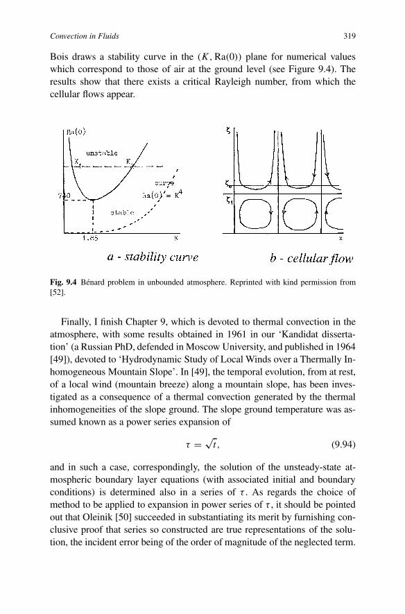
Convection in Fluids 319
Bois draws a stability curve in the (K,Ra(0)) plane for numerical valueswhich correspond to those of air at the ground level (see Figure 9.4). Theresults show that there exists a critical Rayleigh number, from which thecellular flows appear.
Fig. 9.4 Bénard problem in unbounded atmosphere. Reprinted with kind permission from[52].
Finally, I finish Chapter 9, which is devoted to thermal convection in theatmosphere, with some results obtained in 1961 in our ‘Kandidat disserta-tion’ (a Russian PhD, defended in Moscow University, and published in 1964[49]), devoted to ‘Hydrodynamic Study of Local Winds over a Thermally In-homogeneous Mountain Slope’. In [49], the temporal evolution, from at rest,of a local wind (mountain breeze) along a mountain slope, has been inves-tigated as a consequence of a thermal convection generated by the thermalinhomogeneities of the slope ground. The slope ground temperature was as-sumed known as a power series expansion of
τ = √t , (9.94)
and in such a case, correspondingly, the solution of the unsteady-state at-mospheric boundary layer equations (with associated initial and boundaryconditions) is determined also in a series of τ . As regards the choice ofmethod to be applied to expansion in power series of τ , it should be pointedout that Oleinik [50] succeeded in substantiating its merit by furnishing con-clusive proof that series so constructed are true representations of the solu-tion, the incident error being of the order of magnitude of the neglected term.

320 Some Atmospheric Thermal Convection Problems
Fig. 9.5a Initial evolution of the ‘mountain breeze’. Reprinted with kind permission from[49].
Fig. 9.5b Intermediate evolution of the mountain slope wind. Reprinted with kind permissionfrom [49].

Convection in Fluids 321
Fig. 9.5c Global effect of the mountain slope wind. Reprinted with kind permission from[49].
Obviously, it would be futile to expect the method to do something beyondits scope, using it to obtain the steady-state limit solution! For instance, forperturbation of the temperature θ , horizontal component ϕ and vertical com-ponent σ of the velocity vector, we derive from the starting equations thefollowing set of equations for the terms in power series of τ : θ0, θ6, ϕ0, ϕ1,ϕ6, σ0):
∂2θ0
∂s2+ 2s
∂θ0
∂s− 4θ0 = 0, θ0|s=0 = f00(ξ), θ0|s=∞ = 0; (9.95a)

322 Some Atmospheric Thermal Convection Problems
∂2θ6
∂s2+ 2s
∂θ6
∂s− 16θ6 = 4
(ϕ0∂θ0
∂ξ+ σ0
∂θ0
∂s
); (9.95b)
∂2ϕ0
∂s2+ 2s
∂ϕ0
∂s− 8ϕ00 = −4Xθ6, ϕ0|s=0 = 0, ϕ0|s=∞ = 0; (9.95c)
∂2ϕ1
∂s2+ 2s
∂ϕ1
∂s− 10ϕ1 = 8A0
∂
∂ξ
[Z
∫ s
∞θ0 ds
]; (9.95d)
∂2ϕ6
∂s2+ 2s
∂ϕ6
∂s− 20ϕ6 = −4Xθ6 + 4
(ϕ0∂θ0
∂ξ+ σ0
∂ϕ0
∂s
); (9.95e)
∂σn
∂s= −∂ϕn
∂ξ, n = 0, 1, 6. (9.95f)
In these equations the vertical coordinate s = ζ/2τ where ζ is the verticalcurvilinear coordinate directed along the outer normal to the slope and thecurvilinear coordinate ξ is the abcissa along the slope surface (ζ = s =0). The coefficients A0, X and Z are dimensionless scalars that are linkedwith the geometry of the mountain slope. The function f00(ξ) simulates thetemperature distribution (for θ) along the slope. In various parts of Figure 9.5above, the evolution of a local wind, along the mountan slope, under thedouble action of the slope and the thermal field at the slope is represented.
In Figures 9.5a and b, the continuous, boldface lines are relative to hori-zontal (a) and vertical (b) components of the wind. In Figure 9.5c the boldlines (a) are relative to temperature and (b) and (c) are relative to horizontaland vertical components of the wind.
We conclude this chapter with a special mention of the book by Monin[51], where the reader can find, in chapter 8, a pertinent account of the var-ious problems relative to atmospheric general circulation. We also mentionthe book by Boubnov and Glolitsyn [52], where the ‘Convection in RotatingFluids’ is investigated. Finally, in [53] an asymptotic theory of Boussinesqwaves in the atmosphere is presented.
References
1. M.G. Velarde and Ch. Normand, Convection. Scientific American 243(1), 92–108, 1980.2. L.N. Gutman, Introduction to the Nonlinear Theory of Mesoscale Meteorological
Processes. Israel Program for Scientific Translations, Jerusalem, 1972 [translated fromRussian].
3. K.A. Emanuel, Amospheric Convection. Oxford University Press, New York, 1994.4. R.Kh. Zeytounian, Topics in Hyposonic Flow Theory. Lecture Notes in Physics, Vol. 672,
Springer-Verlag, Berlin/Heidelberg, 2006.
Convection in Fluids 323
5. R.Kh. Zeytounian, Meteorological Fluid Mechanics. Lecture Notes in Physics, Vol. m5,Springer-Verlag, Heidelberg, 1991.
6. R.Kh. Zeytounian, On the foundations of the Boussinesq approximation applicable toatmospheric motions. Izvestiya ‘Atmospheric and Oceanic Physics’ 39, Suppl. 1, S1–S14, 2003.
7. I.A. Kibel, An Introduction to the Hydrodynamical Methods of Short Period WeatherForecasting. Macmillan, London, 1963 [translated from Russian].
8. B.S. Dandapat and P.C. Ray, Int. J. Non-Linear Mech. 28(5), 489–501, 1993.9. A.Kh. Khrgian, Physics of the Atmosphere. Gos-Tekh-Izdat, Moscow, 1953.
10. F.T. Smith, J. Fluid Mech. 57(4), 803–824, 1973.11. F.T. Smith, R.I. Sykes and P.W.M. Brighton, J. Fluid Mech. 83(1), 163–176, 1977.12. R.I. Sykes, Proc. Roy. Soc. London A361, 225–243, 1978.13. R.Kh. Zeytounian, Les modèles asymptotiques de la mécanique des fluides, II. Lecture
Notes in Physics, Vol. 276, Springer-Verlag, Berlin/Heidelberg, 1987.14. F.T. Smith, P.W.M. Brighton, P.S. Jackson and J.C.R. Hunt, J. Fluid Mech. 113, 123,
1981.15. R.Kh. Zeytounian, Asymptotic Modelling of Fluid Flow Phenomena. Kluwer Academic
Publishers, Dordrecht, 2002.16. H. Schlichting, Berechnung ebener periodisher Grenzschichtströmungen. Phys. Z.,
33(8), 337, 1932.17. R.Kh. Zeytounian, Convection naturelle périodique au-dessus d’une surface courbe. J.
Méc. (France) 7(2), 231–247, 1968.18. J.M. Noe, Sur une theorie asymptotique de la convection naturelle. Thèse de Doctorat de
3ème Cycle, Université des Sciences et Techniques de Lille I, No. d’ordre 884, March1981.
19. N. Riley, Oscillating viscous flows. Mathematika 12, 161–175, 1965.20. J.T. Stuart, Double boundary layers in oscillatory viscous flow. J. Fluid Mech. 24(4),
673–687, 1966.21. H.E. Fettis, On the integration of a class of differential equations occuring in boundary-
layer and other hydrodynamic problems. In Proc. 4th Mid West Conference on FluidMechanichs, Purdue University, pp. 93–114, 1955.
22. J.E. Simpson, Sea Breeze and Local Winds. Cambridge University Press, 1994.23. J.E. Walsh, Sea breeze theory and applications. J. Atmos. Sci. 31, 2012–2026, 1974.24. H. Niino, On the linear theory of land and sea breeze circulation. J. Meteorol. Soc. Japan
65, 901-921, 1987.25. R.A. Pielke, A comparaison of three-dimensional and two-dimensional numerical pre-
diction of sea breezes. J. Atmos. Sci. 31, 1577–1585, 1974.26. Y. Maher and R.A. Pielke, The effects of topography on sea and land breezes in a two-
dimensional numerical model. Mon. Weather Rev. 105, 1151–1162, 1977.27. J.R. Garrat and W.L. Physick, Beitr. Phys. Atmos. 59, 282–300, 1986.28. J.R. Garrat and W.L. Physick, Beitr. Phys. Atmos. 60, 88–102, 1987.29. Z. Xian and R.A. Pielke, J. Appl. Meteorol. 30, 1280–1304, 1991.30. R.A. Pielke, Mesoscale Meteorological Modeling. Academic Press, Orlando, 1984.31. R.Kh. Zeytounian, Étude Hydrodynamique des Phénomènes Mésométéorologiques.
L’École de la Météorologie, Direction de la Météorologie Nationale, Paris, 1968.32. F.J. Robinson, S.C. Sherwood and Y. Li, J. Atmos. Sci. 65, 276–286, January 2008.33. S. Chandrasekhar, Hydrodynamic and Hydromagnetic Stability. Clarendon Press, Ox-
ford, 1961.34. P.-A. Bois and A. Kubicki, A theoretical model for double diffusive phenomena in cloudy
convection. Ann. Geophys. 21, 2201–2218, 2003.

324 Some Atmospheric Thermal Convection Problems
35. N.E. Veremei, Yu. Dovgalyuk and E.N. Stankova, Izvestiya, Atmospheric and OceanicPhysics 43(6), 731–744, 2007.
36. W.P. Jones and B.E. Launder, Int. J. Heat Transfer 16, 1119–1130, 1973.37. E.N. Stankova, In Proc. Conference of Young Scientists and Specialists of the Voeikov
Main Geophys. Observ., Leningrad, pp. 47–53, 1990 [in Russian].38. R.Kh. Zeytounian, Theory and Applications of Viscous Fluid Flows. Springer-Verlag,
Berlin/Heidelberg, 2004.39. R.S. Scorer, Environmental Aerodynamics. Wiley, 1978.40. J.R.C. Hunt, Environmental Fluid Mechanics. IUTAM Conference, pp. 13–31, 1980.41. G.S. Golitsyn, Simple theoretical and experimental study of convection with some geo-
physical applications and analogies. J. Fluid Mech. 95(3), 567–608, 1979.42. H.T. Rossby, J. Fluid Mech. 36(2), 1970.43. G.S. Kirichenko and P. Poritskiy, Thermocapillary analogue of Rossby waves. At-
mospheric and Oceanic Physis 31(5), 608–610, April 1996 [English translation].44. Zhang Meigen, Linear model of air flow distortion by the effect of breeze. Atmospheric
and Oceanic Physis 31(6), 787–791, June 1996 [English translation].45. R.Kh. Zeytounian, Sur une formulation rigoureuse du problème de la convection libre
atmosphérique. J. Engng. Math. 11(3), 241–247, July 1977.46. R.Kh. Zeytounian and A. Mahdjoub, Prise en compte d’une sous-couche de dissipation
dans les phénomènes de convection libre. ZAMP 40, 931–939, November 1989.47. P.A. Bois, Effets dissipatifs dans les écoulements atmosphériques. Deuxième partie: In-
stabilité linéaire convective dans l’atmosphère. J. Méc. (France) 18(4), 633–660, 1979.48. M.J. Manton, Convection in the lower atmosphere. Austr. J. Phys. 27, 495–509, 1975.49. R.Kh. Zeytounian, Hydrodynamical study of the initial stage of the development of local
winds. Doctoral Thesis, Trudy of the World Meteo Centre, Vol. 3, pp. 19–74, 1964 [inRussian].
50. O.A. Oleinik, PMM 33(3), 441, 1969 [in Russian].51. A.S. Monin, Fundamentals of Geophysical Fluid Dynamics. GidrometeoIzdat,
Leningrad, 1988 [in Russian, but an English translation is available].52. B.M. Boubnov and G.S. Golitsyn, Convection in Rotating Fluids. Fluid Mechanics and
Its Applications, Vol. 29, Kluwer Academic Publishers, Dordrecht, 1995.53. P.A. Bois, Asymptotic theory of Boussinesq waves in the atmosphere. In: Lecture in
CISM Course, Udine (Italy), October 1983. Publ. IRMA, Université de Lille-I, Vol. VI,Fasc. 4, No. 2, pp. II.1 to II.89, 1984
Chapter 10Miscellaneous: Various Convection ModelProblems
10.1 Introduction
It is obvious that the reader, after having digested the preceding ninechapters of this book, will know that many convection phenomena in fluidshave not been considered in our discussion! But this is ‘inevitable’ becauseconvection is a very ‘broad’ subject with many and various facets. It istrue that, for convection in liquids, it has been relatively easy to define thescope of Chapters 3 to 7 in a sensible way, restricting ourselves to threemain facets (as thoroughly discussed in Chapter 8) of the classical Bénardconvection problem, heated from below. However, in the cases when weconsider gases, liquid mixtures, the effect of surfactants, dipolar fluid, orother complementary effects (Dufour and Soret, evaporation, surface activeagents, etc.), a clear definition of a precise method for a rational treatment ofthese various cases is shown to be a difficult affair; obtaining correspondingmodel equations has often, unfortunately, had to be carried out in an ad hocmanner! Despite the inconsistency of these models, the valuable rigourousmathematical results (see, for instance, the book [1] by Straughan, whichpresents rigorous convection studies, mainly by the ‘energy method’, in avariety of fluid and porous media contexts) obtained for such models are oflittle practical value, mainly because we have no assurance that the derived(or proposed) approximate models are really significant and or consistent?
In fact, we are faced with an essential problem of ‘confidence’ concerningthis modeling approach that is intended to be an aid to numerical simulation!
My aim in writing this book has been to present the fundamentals, and toattain this goal it has been necessary to limit the material covered by selecting
325
326 Miscellaneous: Various Convection Model Problems
problems that illustrate unity in convection phenomena and at the same timeput forward its essentials. Consequently, a number of important aspects ofconvection in fluids have ben omitted. In spite of this, the reader can findhere in Sections 10.2 to 10.9 some interesting convection model problems,giving a more complete idea of the wide range of phenomena relative toconvection in fluids and also the vast possibilities to apply rational analysisand asymptotic modelling.
In Section 10.2, the convection problem in the Earth’s outer core is con-sidered and, in particular, we analyze the paper of Jöhnk and Svendsen [2]and give some information concerning this convection problem. Section 10.3is devoted to various comments related to the magneto-convection, electro-thermo-convection, ferro-hydrodynamic convection, chemical convection,solar convection, oceanic circulation and penetrative convection which havemainly been inspired by Straughan’s book [1], and also by various surveypapers relative to the convection problems mentioned above, which havebeen published in Annual Review of Fluid Mechanics (Palo Alto, Califor-nia, USA). Section 10.4 is devoted to a brief discussion of the ‘averaged,integral boundary layer (IBL)’, technique for the non-isothermal case, firstconsidered by Zeytounian [3] and subsequently improved by Kalliadasis etal. in [4], and in two recent papers [5, 6]; here I give my personal opinionand a short ‘history’ of events. In Section 10.5, the results of Golovin etal. [7] and also Kazhdan et al. [8], where the existence of two monotonicmodes (short-scale mode and long-scale mode) of surface tension drivenconvective instability is obtained, is discussed. Section 10.6 concerns ther-mosolutal convection, when the density varies both with temperature andconcentration/salinity, and the corresponding diffusivities are very different(double-diffusive convection [9]), Pr being quite different from Sc; this is,for instance, essential in solidifying alloys (inferior metal mixed with goldor silver), where the interface rejects a solute into the liquid phase. The maintheoretical sources here are the papers by Coullet and Spiegel [10], Knoblochet al. [11], and Proctor and Weiss [12]. In Section 10.7, as a complement toChapter 9, we consider the so-called ‘anelastic (deep) approximation for theatmospheric thermal convection’ – the derivation of these anelastic dissipa-tive deep equations adapted for an atmospheric (deep, viscous, non-adiabaticcase) convection problem, is inspired by our monograph [13, chapter 10, sec-tion 10.2]. In Section 10.8 an interesting convection, initial-boundary valueproblem is linked with a thin liquid film over a cold/hot rotating disk, ac-cording to Dandapat and Ray [14], where the matching between inner (forshort time, near t = 0) and outer (for evolution time, far from t = 0) isaccurately performed; this latter paper has proved to be a valuable prototype

Convection in Fluids 327
problem for many other unsteady film problems. In Section 10.9, solitarywave phenomena in a convection regime are discussed in view of the resultsobtained, in particular by Christov and Velarde [15], and also by Rednikovet al. [16]. Finally, in Section 10.10, some complementary references andcomments concerning some other convection phenomena are given.
This chapter, with various complementary convection phenomena, mightbe itself the subject of a full book. Nevertheless, limiting my investigationsto Sections 10.2 to 10.9 mentioned above, I have considered Chapter 10 as a‘useful informative extension’ of the main part of this book, where the readeris invited to survey the vast panorama of the ‘convection world’.
In the following sections, my approach is the same, but at the same timein some sections I do not have the possibility to develop a detailed rationalanalysis and an asymptotic modelling. Readers should expect to find theremany unresolved questions which might be subject to careful theoretical re-search, but also to various modes of personal reasoning!
10.2 Convection Problem in the Earth’s Outer Core
The Earth’s magnetic field is generally thought to be generated by convectionin its outer core, a process influenced among other things by the stratificationpresent in the outer core. The paper [17] by Fearn and Loper give interestinginformation concerning the compositional convection and stratification in theEarth’s fluid core and the book [18] by Melchior is devoted to the ‘Physicsof the Earth’s Core’. Concerning the ‘Dynamics of the Earth’s Inner andOuter Cores’, see the paper by Smylie and Szeto [19]. In Stacey’s book [20],the reader can find ‘Applications of Thermodynamics to Fundamental EarthPhysics’.
In a review article by Jöhnk and Swendsen [2], a thermodynamic formu-lation of the equations of motion and buoyancy frequency for Earth’s fluidouter core is given. These authors present a precise formulation of the bal-ance and constitutive relations appropriate to the modeling of the motion ofa fluid outer core, including a full thermodynamic analysis and derivation ofbuoyancy frequency and its role in the equations of motion for the fluid outercore, and the dependence of this equation on the thermodynamic state of theouter core. By appropriate scaling, a variety of different approximations arisefrom this formulation, using the thermodynamic definition of the buoyancyfrequency. Special interest is put on scaling for the outer core eigenmodesyielding consistent formulations for the Boussinesq, and the subseismic, ap-

328 Miscellaneous: Various Convection Model Problems
proximation. The starting equations of motion take into account the Coriolisand centrifugal acceleration terms (the fluid is rotating) and also the grav-itational acceleration, g = ∇G, where G is the gravitational potential fora stratified barotropic (p = P(p)) Newtonian fluid with constant bulk andshear viscosity. But, in fact, in the framework of a thermodynamics for atwo-component fluid, the authors consider the specific internal energy as
e = E(S, ρ,C1, C2), (10.1a)
where S and ρ represent the specific entropy and mass density of the mixture(Cα , α = 1, 2, denote the mass fraction of component α in the mixture). Wehave
C1 + C2 = 1 ⇒ C := C1 = 1 − C2 (10.1b)
and
ρdC
dt= −(∇ · i), (10.1c)
which is an evolution equation for mass fraction C of component 1 depend-ing on the divergence of the corresponding mass flux i. We observe that ρCrepresents the partial density of component 1, and equation of state (10.1a)is written as
e = E∗(S, ρ, C). (10.1d)
In particular, using the standard thermodynamic definitions
Ks := ρ
[∂P ∗
∂ρ
]S,C
, where p := ρ2
[∂E∗
∂ρ
]S,C
= P ∗(S, ρ, C),
(10.2a)
γ :=(ρθ
) [∂�∗
∂ρ
]S,C
, where θ :=[∂E∗
∂S
]ρ,C
= �∗(S, ρ, C),
(10.2b)
Cv = θ
[∂�∗/∂S]ρ,C (10.2c)
of the mixture of Grüneisen parameter γ , specific heat at constant volume(and concentration) Cv, and isentropic bulk modulus Ks , respectively, oneobtains the relation (see also [20])
(1
ρ2
)[∂P ∗
∂ρ
]S,C
= ∂2E∗
∂ρ∂S=
[∂�∗
∂ρ
]S,C
= γ θ
ρ. (10.3)
As a result, a complete system of equations of motion for a rotating, gravi-tating, stratified, heat conducting, 2-component Newtonian fluid is derived.
Convection in Fluids 329
As a further result, we have nine differential equations for the nine quan-tities (G, ρ, p, θ, S, C, u); the complexity of the differential equations hasincreased considerably via the incorporation of entropy and concentrationinto the model.
Under realistic physical assumptions for the problem of normal modes,the thermodynamic processes, represented explicitly in a complete systemof equations, can be reduced in essence (according to the authors!) to a sin-gle parameter, i.e., the buoyancy frequency. This complete system, althoughvery complex, does not completely represent an exact thermodynamic de-scription of the Earth’s outer core! On the other hand, the stratification ofa (fluid) system is intimately related to its so-called buoyancy frequency.This buoyancy frequency may be interpreted as the oscillation frequency oreigenfrequency in the system considered below, (In a complicated systemthe oscillation and buoyancy frequencies may no longer coincide, as is thecase in our simple model.) In this model, the expressions ‘stratification’ and‘buoyancy frequency’ will, for simplicity, always refer to N2 (the square ofthe buoyancy or Brunt–Väisälä frequency). Usually, estimates of N2 in theliterature are based on
N2 = −(g
ρ
)[(gρ2
Ks
)+ ρ ′
E
], (10.4)
where in a simple model we can interpret ρ ′E as the density stratification of
the fluid. In [2, pp. 83–89], the reader can find a pertinent discussion con-cerning the ‘stratification and the buoyancy frequency’. The resulting non-dimensional form of the system of nine equations for (G, ρ, p, θ, S, C, u),derived via a dimensional analysis and approximations for core undertones(subdued tones), contain certain non-dimensional numbers, reflecting the or-der of the terms with which they are associated.
The list of characteristic values (Table 10.1) for the outer core (see [18,20]) has been taken from [2, p. 90]. A particularly important simplificationarising out of this non-dimensional analysis is that temperature and concen-tration (to lowest order) play a role in core oscillations only through the de-pendence of the buoyancy frequency on these variables. In addition, the non-dimensional analysis validates the Boussinesq approximation of the balancerelations, in which the general buoyancy frequency discussed above entersas the sole stratification parameter.
This dimensionless analysis is performed by Jöhnk and Svendsen [2,pp. 90–97] and deserves (at least, from my point of view) a further carefulexamination (and maybe a complementary investigation). The main featureis (because the characteristic velocity U is very small ≈ 3 × 10⁻⁴ m/s) re-

330 Miscellaneous: Various Convection Model Problems
Table 10.1 Some characteristic values for the Earth’s outer core. Reprinted with kind per-mission from [2].
Gravitational constant � = 6.67 × 10⁻¹¹ m3 kg−1 s−2
Angular velocity � = 7.3 × 10⁻⁵ s−1
Thickness of the OC L = 2.3 × 10⁶ mVelocity (westward drift) U = 3 × 10⁻⁴ m s−1
Mean gravity [g] = 7.5 m s−2
Mean density [ρ] = 1.1 × 10⁴ kg m−3
Density variation �ρ = 2.3 × 10³ kg m−3
Mean temperature [θ] = 4.4 × 10³ KTemperature variation �θ = 1.2 × 10³ KMean concentration (LEs) [c] = 2 × 10⁻¹
Concentration variation �c = 1 × 10⁻¹
Isentropic bulk modulus [K] = 8.5 × 10¹¹ PaSpecific heat at constant volume [cv] = 6.8 × 10² m2 s−2 K−1
Grüneisen parameter [γ ] = 1.3Thermal expansion [αθ ] = 1.1 × 10⁻⁵ K−1
Thermal conductivity [k] = 3.3 × 101 kg m s−3 K−1
Mass diffusivity [D] = 6 × 10⁻⁹ m2 s−1
Kinematic viscosity [ν] = 1 × 10⁻⁶ m2 s−1
lated to a small Rossby number (see the value of �0 and L in Table 10.1),Ro = U/�0L � 1, leading to an important simplification of the equationsof motion. However, it is now well known [21] that the limiting process,Ro → 0 with time-space coordinates fixed, is very singular in time t (neart = 0 and an adjustment problem must be considered to geostrophy) and alsoon the boundary (Ekman layer problem). With Ro we have also the followingdimensionless parameters:
Ek = [ν]�0L2
,�θ
[θ] ,�ρ
[ρ] ,Ek
Pr= [k]�0L2[Cv][ρ] , (10.5a)
g
4π= L�[ρ]
[g] , C = [Ks][g][ρ]L,
Fr
Ro= �02L
[g] , (10.5b)
which are respectively the Ekman number, relative temperature and densitychange, Ekman–Prandtl number, self-gravitational number, compressibilitynumber and Froude–Rossby number.
In Table 10.2, the magnitude for the above dimensionless numbers aregiven.
In [2, sections 4.2–4.6], the authors consider respectively, ‘Scaling of thebasic fields’, ‘Buckingham � theorem’, ‘Von Zeipel’s (1924) Result’, ‘Di-mensionless, Perturbed Balance’ and ‘Constitutive Relations and Approxi-

Convection in Fluids 331
Table 10.2 Definition and some magnitude for four dimensionless parameters. Reprintedwith kind permission from [2].
[ρ], �ρ density stratification[θ], �θ temperature stratification[Ks] compressibility[g] gravity� self gravitation[cv] heat capacity[k] heat conduction[ν] viscosity[D] diffusionL length� frequencyU velocity
E = [ν]�L2
Ekman number
R = U
�L2Rossby number
T = �θ
[θ] relative temperature change
D = �ρ
[ρ] relative density change
mation’. It seems to me that their approach is not very clear and in any casedoes not lead to a rational derivation of approximate model equations; again,a consistent asymptotic approach is necessary!
But, assuredly, ‘the use of the thermodynamic approximation significantlysimplifies the equations of motion for a heat conducting, two-componentfluid outer core’.
A rational derivation of a set of approximate model equations, inspiredfrom our above discussion, remains a challenging open problem! As a com-plement to [2], the reader can read also the two (now classical) papers byRoberts and Soward [22] and Wood [23].
10.3 Magneto-Hydrodynamic, Electro, Ferro, Chemical, Solar,Oceanic, Rotating, Penetrative Convections
The Boussinesq approximation, which allows one to consider for variousconvection problems a Boussinesquian (à la Boussinesq) fluid, is perhaps themost widely used simplification of convection in fluid modelling. We have al-ready, in preceding chapters of this present book, dealt with this Boussinesqapproximation. In Chapters 3 and 5 it appears in relation to the ‘Rayleigh’simple thermal convection problem and the thermal, à la Rayleigh–Bénard,shallow convection problem. In Chapter 9, we have used this Boussinesq ap-proximation in various parts to formulate atmospheric convection models.Finally, in Section 10.2, the Boussinesq approximation plays a significant

332 Miscellaneous: Various Convection Model Problems
role in the derivation of simplified, approximate, model equations for con-vection in the Earth’s outer core.
A very good illustration of the plurality of the ‘Boussinesquian thermalconvection’ is the numerous survey papers (in various volumes of AnnualReview of Fluid Mechanics) where this Boussinesq approximation is the ba-sis for mathematical formulation of the model problems. Examples are: con-vection in mushy layers [24]; solar convection and magnetic buoyancy [25];magneto-convection [22]; mantle convection [26]; oceanic general circula-tion [27]; convection in rotating systems [28]; convection involving thermaland salt fields [9]; dynamic of Jovian atmospheres [29]; etc. These examplesare applied to a variety of gases and liquids or to more complicated fluidswith various complementary effects.
It is interesting to observe that Oberbeck, before Boussinesq (see [30]),uses a Boussinesq type approximation in meteorological studies of theHadley thermal regime for the trade-winds arising from the deflecting ef-fect of the Earth’s rotation. Concerning this rotating convection, the readercan find recent (1998!) developments in the well-documented paper [31]by Knobloch; this paper is, in fact, a pertinent complement to chapter IIIof the famous book by Chandrasekhar [32], where the effect of rotation onRayleigh–Bénard convection is taken into account (formulated as a stabilityproblem for an infinite layer with rotation parallel to gravity, which involvesseveral assumptions; see for instance the brief discussion in [31, p. 1422]).In [32, chapter IV] the reader can find the effect of a magnetic field onRayleigh–Bénard convection and some details about the effect of Alfvénwaves. In [32, chapter V] the coupled effect of rotation and a magnetic fieldis considered, where the propagation of hydromagnetic waves in a rotatingfluid and onset of thermal instability in the presence of rotation and magneticfield are both investigated. On the other hand, in Straughan’s recent book [1],the reader can find a presentation of nonlinear energy stability results ob-tained in convection problems by means of an integral inequality technique(energy method). In [1, chapter 7], this energy method is systematically de-veloped for geophysical problems (for example, for patterned ground forma-tion) and in [1, chapter 9] for the Bénard problem in the case of a microp-olar fluid. In [1, chapters 11–13], a different line of attack is adopted; thesechapters are concentrated on technologically relevant and relatively new the-ories: dielectric fluids and electro-hydrodynamic/electrothermal-convection,ferro-hydrodynamics convection and chemical convection (for reacting vis-cous fluids far from equilibrium).
More precisely, we consider first the Magneto-Hydrodynamic, MHD,Convection (see [22, 23], and [1, chapter 11]), which is the study of the inter-

Convection in Fluids 333
action between magnetic fields and fluid conductors of electricity. The bodyforce acting on the fluid is the Lorentz force that arises when electric currentflows at an angle to the direction of an impressed magnetic field. The MHDconvection problem is a very important one because it has intrinsic applica-tions to the behaviour of planetary and stellar interiors (see, for instance, thepaper by Hughes and Proctor [25]), and in particular, to the behaviour insideof the Earth (as has been discussed here in Section 10.2).
In MHD convection, the relevant equations may be written (Eulerian case,a perfect plasma and adiabatic motion) as [33]:
ρdU
dt+ 2� ∧ U = ∇p + gρk =
(1
µ
)(∇ ∧ B) ∧ B, (10.6a)
∂B∂t
+ ∇ ∧ (B ∧ U) = 0, (10.6b)
∇ · B = 0, (10.6c)
dρ
dt+ ∇ · U = 0, (10.6d)
dT
dt−
[(γ − 1)
/γ
] [T
p
]dp
dt= 0, (10.6e)
p = RρT, (10.6f)
which is a closed system for p, ρ, T , U and B, the pressure, density, temper-ature, velocity and magnetic induction with constant magnetic permeabilityµ. In dimensionless form in these equations we have five non-dimensionalparameters:
St = L0
t0U0, Ro = U0
2�0L0, M = U0
(γRT0)1/2, Fr = U0
(gL0)1/2,
(10.7a)
A = U0
[B0/(µρ0)1/2] , (10.7b)
the Strouhal, Rossby, Mach, Froude and Alfvén numbers. Below it is as-sumed that A and M are simultaneously very small and satisfy the similarityrelation [34]
A2 = a0M with a0 = O(1) is a constant. (10.8a)
In a quasi-steady case, St = 0, the case when
Fr → 0, such that A2 = b0 Fr2, with b0 = O(1), a second constant,(10.8b)

334 Miscellaneous: Various Convection Model Problems
leads to limit (superscript ‘0’), M = (b0/a0)Fr2 → 0, a static equilibriumapproximation (Ro = ∞; see the paper by Grad [35]) written with dimen-sionless quantities:
(∇ ∧ B0) ∧ B0 =(a0
γ
)∇p1 + b0k (10.9a)
and∇ · B0 = 0, (10.9b)
where p1 = lim[(p − 1)/M] for M → 0. If from ∇ · B0 = 0, we writeB0 = ∇ϕ∧∇ψ , then equation (10.9a) gives B0·∇P = 0, or P ≡ (a0/γ )p
1+b0z = �(ϕ,ψ), and [36]
(∇ ∧ B0) · ∇ϕ = ∂�
∂ψ(10.9c)
and
(∇ ∧ B0) · ∇ψ = −∂�
∂ϕ, (10.9d)
both these ‘first integrals’ (10.9c, d) being equivalent to (10.9a, b). WhenRo = c0A
2 = c0a0M → 0, instead of the two equations (10.9c, d), wederive the following limit equation (from the dimensionless form of (10.6a)):
(1
c0
)(� ∧ U0)+
(a0
γ
)∇p1 + b0k = (∇ ∧ B0) ∧ B0, (10.10a)
and if T 1 = lim[(T − 1)/M] for M → 0, then to the above limit equation(10.10a) we can associate the following set of quasi-steady limit equations[34]:
∇ · U0 = 0 and ∇ · B0 = 0, (10.10b)
∇ ∧ (B0 ∧ U0) = 0, (10.10c)
U0 · ∇T 1 =[(γ − 1)
γ
]U0 · ∇p1, (10.10d)
ρ1 = p1 − T 1, (10.10e)
which are consistent only when (because β = γ (M/Fr)2 ≡ (b0/a0)M → 0)
RT0
g� L0 � U2
0
g. (10.10f)
If Fr → 0 such that β = γ (M/Fr)2 = O(1) then, with (10.8a), a stronglycoupled limit system is derived in [34], similar to a deep convection system,

Convection in Fluids 335
which is adapted to the study of atmospheres in various planets of the so-lar system (and, concerning this problem, see section 23 in Monin’s book[37]) for which the characteristic angular velocity of rotation is not veryhigh (A2/Ro � 1). This model system is well balanced for a description ofmagneto-convective motions within a relatively thick layer (when the gravityis low and reference temperature at the ground is high, then the layer is morethick). Another interesting case is linked with the limit
β = β∗M with β∗ = O(1), (10.10g)
and in this case, as limit steady-state system, we derive a set of model equa-tions which is similar to a Boussinesq system for low Rossby number (see,for instance, [38]). This limit system seems pertinent for a rational analysisof the development of the sun-spot for which the magnetic and convectioneffects are strongly coupled.
Finally, we note that the theory of heavy-magneto-fluids at low Alfvénnumber is very similar to the theory of heavy-rotating-fluids at low Rossbynumber, and on the other hand we observe an analogy between the sta-tic equilibrium approximation (10.9a,b), in MHD, and the classical quasi-geostrophic approximation in dynamic meteorology [37].
Many papers deal also with the effect of a uniform magnetic field on theonset of Bénard–Marangoni convection in a layer of conducting fluid; in Wil-son’s paper [39] the reader can find various references. In particular, a verti-cal magnetic field always has a stabilizing effect, but when the free surfaceis deformable and includes a sufficiently large Marangoni number, it will al-ways have unstable modes no matter how strong the applied magnetic fieldis! In a recent survey paper by Zhang and Schubert [40], the MHD phenom-ena, in rapidly rotating spherical systems, is discussed. (Although this is notthe place for a full dicussion, I would like to mention a particularly interest-ing and singular effect: in the presence of a non-uniform magnetic field, mostclassical fluids – for instance, water and aquous solutions – can exhibit somediamagnetism or paramagnetism and their behavior may be strongly affected(convection suppressed, or convection present when the fluid is heated frombelow).
On the other hand, the domain of MHD effects in liquid metals is alsoquite important, namely when thermo-electric effects (for instance, the See-beck effect) generate an electric current and, as soon as a magnetic field ispresent, results in an electrically driven flow.
Finally, I think that our above investigations can be generalized when instarting equations (10.6a–f) the viscosity and heat conduction are taken into

336 Miscellaneous: Various Convection Model Problems
account. In this case the equations are more complicated but the character-istic Ekman number being small, it is possible to consider a boundary layerapproximation near the wall.
In a paper by Roberts and Soward [22], a complete dimensionless sys-tem of MHD equations is given (see [22, p. 126]). The first use of the en-ergy method in MHD was by Rionero in 1967 (establishing existence of amaximizing solution in the energy variational problem) and in 1971 he alsoincluded the Hall effect.
The linear theory of Chandrasekhar (1981) shows that as the field strengthis increased for the MHD convection problem with the magnetic field per-pendicular to the layer, the magnetic field has a strongly inhibiting effecton the onset of convection motion. The first analyses to confirm this sta-bilizing effect from a nonlinear energy point of view are due to Galdi andStraughan (1985) and Galdi (1985) introduced a highly non-trivial gener-alized energy that contains gradients as well as the fields themselves.Thisenergy has some resemblance to the one needed to obtain stabilization inthe rotating Bénard problem (for references of the above papers by Rionero,Chandrasekhar, Galdi and Straughan, see [1]).
Now, concerning Electro-Hydrodynamic, EHD, Convection, the branch offluid mechanics concerned with electric force effects, this topic is relativelynew and has been attracting increasing attention in the theoretical and engi-neerng literature. Some aspects of this EHD convection are well presentedin Straughan’s book [1, chapter 11], who gives Rosensweig’s [41, pp. 1, 2]explanation:
the force interaction arising in EHD is often due to the free electriccharge acted upon by an electric force field.
In [1], most of the analysis described is via linear instability theory, since en-ergy theory has been so far successful only in certain cases. This is indeed arich area for future research. Roberts [42] first allows the dielectric constantof the fluid to vary with temperature T , and assumes the homogeneous insu-lating fluid at rest in a layer (with d as depth) with vertical, parallel appliedgradients of temperature and electrostatic potential V . The electric displace-ment is denoted by D, and the body force per unit volume f on an isotropicdielectric fluid is given (see in [43, eq. (15.15)] or in [1, p. 163]) as a functionof the pressure p, electrical field E and density ρ, by
f = −∇p +( ρ
8π
)∇
{E2
[∂ε
∂ρ
]T
}−
(E2
8π
) [∂ε
∂T
]ρ
∇T . (10.11a)
The appropriate Maxwell equations are

Convection in Fluids 337
∇ · D = 0, curl E = 0 with D = ε(ρ, T )E and E = −∇V . (10.11b)
For a Newtonian fluid, from a similar to a Boussinesq approximation,Roberts considers the following equations (ui are the components of the ve-locity vector u):
∂ui
∂t+ uj
∂ui
∂xj= gi + ν�ui, (10.11c)
with
gi = − ∂ω
∂xi−
(1
ρ0
)(E2
8π
)[∂ε
∂T
]ρ
∂T
∂xi− g[1 − α(T − T0)]ki , (10.11d)
g being gravity, α the thermal expansion coefficient, and k = (0, 0, 1), with
ω =(p
ρ0
)−
(E2
8π
)[∂ε
∂ρ
]T
. (10.11e)
For the given T we have
∂T
∂t+ uj
∂T
∂xj= κ�T , (10.11f)
κ being the thermal diffusivity.It seems to me that the first problem in the framework of a rational analysis
and asymptotic modelling is to derive, with (10.11a), for f – as a phenomeno-logical relation – a dimensionless system in the compressible, viscous andheat conducting with viscous dissipation case. Then one can verify whetherthe above Roberts, approximate (ad hoc) system is really derived. Unlesssuch a procedure is implemented, it seems to me that it is difficult to trust thefurther results of Roberts in [1, chapter 11].
Another approximate model was also considered by Turnbull [44], which,curiously, considers that:
Ohm’s law (J is current and Q the volume space charge),
J = σE +Qu, with charge conservation, ∂Q/∂t + ∇ · J = 0,(10.11g)
is only an approximation for poorly conducting liquids, and, therefore, itmakes no sense to solve the equations exactly since the model is only anapproximation! A third contribution was made by Deo and Richardson [45]which considers a generalized energy method in EHD stability theory. Ac-cording to Straughan:

338 Miscellaneous: Various Convection Model Problems
. . . the paper [45] represents a substantial contribution to energy stabil-ity theory, especially since, as far as I can determine, it is the first toaddress the very interesting EHD problem.
The authors of [45] work with dimensionless quantities and introduce var-ious non-dimensional parameters, in this case the governing equations ofthe considered problem (‘charge injection induced instability and the non-linear energy stability analysis’; see [1, section 11.4]) admit a steady one-dimensional hydrostatic equilibrium solution with the equilibrium electricpotential. As a consequence, a system of equations for perturbations in liq-uid velocity, electric field and space-charge density is derived in [45, pp. 173,174]. From my point of view, precisely the consistency of this system (mak-ing sure that all the terms in equations of this system are the same orderof magnitude) is an interesting problem in a framework of a rational analy-sis and asymptotic modelling. Only in this case do the results of Deo andRichardson really represent a ‘substantial contribution’!
Now, Ferro-Hydrodynamic, FHD, Convection, which is the subject ofchapter 12 in [1], is of great interest because the fluids of concern possess (asis written in [1]) a giant magnetic response, as a consequence, in particular, ofa spontaneous formation of a labyrinthine pattern in thin layers and, also, theenhanced convective cooling in a ferrofluid that has a temperature-dependentmagnetic moment. The book by Rosensweig [41] is a perfect introduction tothis fascinating subject, and in [1, chapter 12] the reader can find the ‘relevantbasic equations of FHD’. It seems that the papers by Cowley and Rosensweig[46] and Gailitis [47] are interesting for the problem of interfacial stabilityof a ferromagnetic fluid. On the other hand the temperature dependence ofmagnetization is important in thermo-convective instability in FHD.
Chapter 13 of [1] is devoted to ‘Chemical Convection’. In particular, thephenomenon of double-diffusive convection in a fluid layer, where two scalarfields (see Section 10.5 here, where these scalar fields are heat and salinityconcentration) affect the density in fluid, is closely related to this CC; thebehaviour in the double-diffusive case is often more diverse than for the Bé-nard classical convection problem. But, when temperature and one or morespecies are present and interactions between species are allowed, then thesystem becomes increasingly richer (see, for instance, the comments in [48]);as a consequence, reaction-diffusion equations for mixtures of viscous fluidsplay an important role in everyday life.
Unfortunately, the relevant equations for various cases are usually writtendown in an ad hoc manner and often vary considerably. A rational derivationof a consistent system of model equations would seem appropriate, and in

Convection in Fluids 339
[1, chapter 13], the reader can find some results in this direction, i.e., basicequations for a chemical reacting mixture (according to Morro and Straughan[49]), a model for reactions far from equilibrium and convection in a layer.
Finally, we note that recently in [50] the authors are interested in the in-fluence of Marangoni effects on the propagation of chemical fronts in thinsolution layers, open to the air, in the absence of any buoyancy- driven ef-fects.
Many fascinating solar phenomena (in particular, Solar Convection) canbe attributed to the influence of the Sun’s magnetic field, well described inthe review paper of Hughes and Proctor [25]. According to this paper:
The interior of the Sun (which has a radius of 7 × 10⁵ km) is dividedinto three main sections – an inner core (occupying 25% by radius)in which the (thermo)-nuclear reactions take place, an intermediate re-gion (extending to approximately 70% of the solar radius) where heatis transported by radiation, and an outer region where heat is carried byconvective motions.
In [25] the authors are concerned with the magnetic field in, and just below,the convection zone and they concentrate their investigations only on twoparticular facets of solar magneto-hydrodynamics: first, on the behaviour ofa vertical field in the surface layers of the Sun and, second, on the evolutionof a horizontal field in somewhat deeper regions.
The complex dynamo mechanism by which the field is regenerated andthe effects due to solar rotation are not considered in [25]. The interestingfeature is the convection in the surface layers of the Sun which is domi-nated by cells of two discrete scales: granules with average size 1500 km,and supergranules that are about 20 times as large. It is postulated that be-neath these cells the heat will be transported by giant cells spanning almostthe entire depth of the convection zone! The use of Boussinesq approxima-tion does not permit discussion of several important phenomena. In fact, theconvection zone of the Sun is highly turbulent and the fields within it highlyintermittent; the time scale for changes in the granulation pattern is only 15minutes or so, and that for the supergranulation pattern a few hours. In anycase, it is hard to justify a theory in which viscosity (presumably turbulent) isretained while magnetic diffusivity (typically of comparable size) is ignored!
More recent work has attempted to set the problem of flux-sheet concen-tration and evacuation in the context of a proper treatment of nonlinear com-pressible convection in the framework of the full equations – for instancein [25, eqs. (2.1)–(2.5), pp. 189–190], describing convection in the outer re-gions of the Sun. However, it seems that a full theory of radiative transfer is

340 Miscellaneous: Various Convection Model Problems
required to give a correct model of convection (with or without a magneticfield) in the surface layers of the Sun! In fact, equations (2.1)–(2.5) in [25]are extremely complicated, even in the absence of a magnetic field. We ob-serve also that the curvature forces exerted by the magnetic field can lead tothe propagation of waves along field lines (giving an oscillatory convection).In [25] the reader can find various pertinent references up to 1987.
Again in [1, chapter 18], the reader can find a review of the application ofnonlinear stability in Ocean Circulation Models. In [1], first the stability ofwind-driven convective motions in the upper layers of the ocean – known asLangmuir circulations – is considered in the framework of the Lebovich andPaolucci paper [51]. Then, the Stommel–Veronis (quasi-geostrophic) modelis considered in [1, chapter 18, according to a series of papers by Criscianiand his co-workers relative to nonlinear energy stability (see, for instance[52]). This quasi-geostrophic model is relative to a streamfunction of two-dimensional motion and is developed and discussed in detail in chapter 2 ofPedlosky’s book [53].
On the other hand, the review paper by McWilliams [27] is devoted tohistory, formulation and solution of numerical models for oceanic generalcirculation under equilibrium surface wind stress and buoyancy flux forc-ing. In the framework of the theory of convection in fluids, obviously thefundamental fluid dynamics equations of oceanic circulation are the Navier–Stokes(–Fourier) equations on the rotating Earth for a compressible liquid,seawater, which is comprised of water plus a suite of dissolved salts thatoccur in nearly constant ratio but variable amount (the salinity s), with anempirically determined equation of state. In fact, the model equations used(see, for instance, the very pertinent paper [54] by Veronis, who considersthe ‘large amplitude Bénard convection in a rotating fluid’) are based onseveral substantial simplifications to this above-mentioned fundamental set!An interesting convection aspect is the ‘buoyancy-driven circulation’, as thegeographical patterns of buoyancy forcing differ for heat and fresh water.Tropical heating and polar cooling tend to force a circulation with sinking athigh latitudes, whereas tropical excess evaporation (largest somewhat awayfrom the equator) and polar excess precipitation tend to force sinking at lowlatitudes. This creates the possibility of multiple equilibria with alternativeoverturning circulation patterns.
It is necessary to observe that quasi-geostrophic approximation, large-scale (planetary) geostrophic equations, balance equations, and primitiveequations are usually used for atmospheric motions; see, for instance, thebooks [13, 55] and also [21], where these model equations are derived froma careful rational analysis coupled with an asymptotic modelling. I think that

Convection in Fluids 341
such a consistent approach is also possible in the problem of the derivationof model approximate equations for oceanic circulation – a remarkable (andrather unusual; see, for instance, our recent paper [56]) aspect of such anapproach is the possibility (by asymptotic matching) to associate to the mainnon-adiabatic, dissipative hydrostatic (N-A DH) model evolution equations,two local systems of model equations – on the one hand near the initial time(for an unsteady adjustment (UA) and, on the other hand for a meso- scaleprediction (which takes into account the influence of the vertically propagat-ing gravity waves (M-SP)).
The N-ADH main equations are derived via the limit process:
ε = H
L→ 0 and Re = UL
ν→ ∞, such that ε2 Re = O(1),
(10.12a)or
L ≈(U
ν
)H 2, (10.12b)
for the velocities (uM, vM,wM), pressure pM , density ρM and temperatureTM , with the space-time dimensionless coordinates (t, x, y, z) fixed andO(1). More precisely,
x = a cos ϕ0λ, y = a(ϕ − ϕ0), z = r − a, (10.12c)
where ϕ0 is a reference latitude – the origin of this right-handed curvilinearcoordinateless system lies on the Earth’s surface (for a flat ground we haver = a) at latitude ϕ0 and longitude λ = 0.
The UA local equations, valid near initial time, are derived also from(10.12a), for the velocities (ul = uM , vl = vM , and wl = εwM), pres-sure pl = pM , density ρl = ρM and temperature Tl = TM , but with a shortdimensionless time
τ = t
ε2and space coordinates x, y, ζ = z/ε fixed and O(1). (10.12d)
The M-SP local equations, valid in a meso-scale region situated around thepoint (x0, y0, z = 0), are also derived from (10.12a), for (ul, vl, wl), pl , ρland Tl , but, as functions of τ ∗ and x∗, y∗ and z fixed and O(1), where
τ ∗ = t
ε, x∗ = (x − x0)
ε, y∗ = (y − y0)
εand z are fixed and O(1).
(10.12e)In particular, both of the above local models, with (10.12d) and (10.12e),
give by matching the possibility to obtain, on the one hand, consistent initial

342 Miscellaneous: Various Convection Model Problems
conditions for the main N-ADH model with (10.12a, b) for a ‘large’ weatherprediction and, on the other hand, the required lateral (horizontal) conditionsat infinity for the meso-scale-regional prediction, once the large weather pre-diction by N-ADH model is known at the position (x0, y0, z = 0). This al-lows us to take into account the meso-scale topographic roughness whichalso influences large-scale circulation (neglected in the large weather predic-tion by the N-ADH model).
Finally, concerning the problems related to the atmospheric and oceanicgeneral circulations, see chapter 8 in Monin’s book [57]; on the other hand,the book by Marchuk and Sarkisyan [58] gives a very pertinent and completeaccount of various computational algorithms for numerical simulations ofocean circulation.
Concerning Rotating Convection, see the two references in the beginningof Section 10.3. The article by Knobloch [31], cited there for work as recentas 1998, is a pertinent complement to chapter III of Chandrasekhar’s famousbook [32]. Knobloch summarizes some of the developments (up to 1996)in bifurcation theory and their relevance to the study of rotating convection.From the point of view of these authors:
. . . undoubtedly, the most fundamental property of rotating systems isthe absence of steady-state bifurcations. As a result patterns in rotatingsystems invariably precess.
In [31] the author noted that this fact is related to the absence of reflectionsymmetry in vertical planes in such systems, and pointed out that the impo-sition of translation invariance in addition to rotation invariance changes theabove picture in a dramatic way.
In [31, section 2], relative to convection in a rotating cylinder, the authorwrites for the case of small Froude numbers the equations of motion, non-dimensionalized with respect to the thermal diffusion time in the vertical, inthe following form:[(
1
Pr
)D
Dt− ∇2
]u = −∇p + Ra�k + 2�0u ∧ k, (10.13a)
[D
Dt− ∇2
]� = w, (10.13b)
∇ · u = 0, (10.13c)
where u = uer + veϕ + wk is the velocity field, � and p are the departuresof the temperature and pressure from their conduction profiles, and k is theunit vector in the vertical direction. In equation (10.13a) we have

Convection in Fluids 343
�2 ≡ d2�phys
ν, Ra ≡ gα�T d3
κν,
1
Pr≡ κ
ν, (10.13d)
�0 being the dimensionless angular velocity. We observe that, only when theFroude number d(�phys)
2/g is small, one can suppose that gravity is essen-tially vertical everywhere within a domain of characteristic size d. In [31],Knobloch considered an interesting nonlinear regime, perhaps the most in-teresting phenomenon in a rotating layer, the Küppers–Lortz (KL) instability(see [59]; this KL instability is, in fact, related to the absence of reflectionsymmetry in vertical planes in horizontally unbounded layers). When insta-bility in a pattern of parallel rolls becomes unstable to another set of rollsoriented at an angle with respect to the first, once the rotation rate exceeds acritical value, this new set is itself unstable in the same fashion, etc., resultingin complex dynamics right at the onset. In [31] Knobloch discusses the KLinstability for traveling waves and shows that structurally stable heterocliniccycles involving traveling roll states are possible, and result in quite unusualdynamical behavior.
Concerning the theory of dynamical systemm and chaos, the reader canconsult the book by Wiggins [60]. In [61], the reader can find numerous ref-erences and comments concerning various aspects of the rotating Rayleigh–Bénard convection, for instance, rotating about a vertical axis [62, 63], pat-tern formation [64], direct transition to turbulence [65], pattern dynamics[66], and chaotic domain structure [67].
Furthermore, concerning stability results, I mention the paper by Muloneand Rionero [68] where new stability results for any Prandtl and Taylor num-bers are obtained.
Finally, concerning Penetrative Convection, we mention the book ofStraughan [69] devoted to ‘mathematical aspects’ and also chapter 17 of hismore recent book [1] where, at the beginning of this particular chapter, theauthor pertinently writes
A pioneering piece of work on penetrative convection is the beautifulpaper (1963) of Veronis [70].
From the physics’ point of view, there are many geophysical and astrophys-ical settings which involve a layer of gravitationally stable fluid, boundedabove or below by a layer which is in convective motion. A typical exam-ple is the case of the Earth’s atmosphere bounded below by the ground (orocean). This bounding surface is heated by solar radiation, and the air closeto the surface then becomes warmer than the upper air, and so a gravitation-ally unstable system results; when convection occurs, the warm air rises andpenetrates into regions that are stably stratified.

344 Miscellaneous: Various Convection Model Problems
There are various ways to obtain the penetrative effect of convection. First,if one assumes (as Veronis does in [70]) that the equation of state is no longerlinear in the temperature, one introduces a ‘non-Boussinesq’ effect. A sec-ond way is to assume, as in a classical Boussinesq approximation case, thatthe density is linear in the temperature field, but introduce an internal heatsource in the layer via the equation for the temperature. A third way is, infact, the case similar to the atmospheric case when the lower bounding sur-face is heated by a radiating heating. For instance in a usual Rayleigh–Bénardshallow convection system of equations, as a boundary condition for the tem-perature T , at z = 0, we write a heat flux condition (with q0 = const)
κ∂T
∂z
∣∣∣∣z=0
= κq0, (10.14)
and when q0 > 0, this means heat is being taken out of the fluid layer,whereas q0 < 0 means that heat is being put into the fluid layer through theboundary z = 0.
Obviously, in a more general case, the three cases discussed above can becombined; in particular, I invite the reader to read [1, pp. 347, 348], where abeautiful experiment (performed by Krishnamurti [71]) is described.
A fourth way to study penetrative convection is via a multi-layer theory,by assuming there are two (or more) layers present with different temperaturegradients, at least one being destabilizing, with suitable boundary conditionsat the interface(s).
Penetrative convection in fluid layers with internal heat sources is con-sidered by Ames and Straughan in [72]. Penetrative convection in the upperocean due to surface cooling is the subject of a paper by Cushman-Roisin[73]. Denton and Wood [74] consider penetrative convection at low Pécletnumber. Numerical studies of penetrative convective instabilities are consid-ered by Faller and Kaylor in [75]. For the penetrative convection in porousmedia, see the paper by George et al. [76]. Penetrative convection in rotatingfluids, a model for the base of stellar convection zones, is considered by Jen-nings in [77]. Penetrative convective flows induced by internal heating andmantle compressibility is investigated by Machetel and Yuen in [78]. For amodel for the onset of penetrative convection, see Matthews [79]. Nonlinearpenetrative convection is studied by Moore and Weiss in [80]. In [81], Strausconsiders penetrative convection in a layer of fluid heated from within, andZahn et al. in [82], perform a nonlinear modal analysis of penetrative con-vection.

Convection in Fluids 345
10.4 Averaged Integral Boundary Layer Approach:Non-Isothermal Case
We have already explained, in Section 7.5, the main point of the ‘averaged,integral boundary layer (IBL)’ technique, for isothermal (Shkadov in 1967[83]) and non-isothermal cases (first considered by Zeytounian in 1998 [3],see the system (7.94a–c) in Section 7.5). In fact, the non-isothermal system(7.94a–c) was derived in 1995 (during our employment at the LML of theUniversity ST of Lille) in the framework of our research related to obtainingfinite-dimensional dynamical-system models for numerical simulation of thedestabilizing Marangoni effect on route to chaos and in appearance of strangeattractors (see, for instance [3, section 4.4]). Thanks to an invitation fromProfessor Manuel G. Velarde, Director de la Unidad de Fluidos del InstitutoPluridisciplinar de la Universidad de Madrid (Spain), in November 1999, Ihad the opportunity to expound a part of this research, including obtainingof this system of non-isothermal averaged equations, similar to (7.94a–c),which, from my point of view, is of unquestionable interest for investigationof the destabilizing Marangoni effect. Curiously, in 2003, Kalliadasis et al.[84] also considered the non-isothermal case but did not mention my 1998approach; these authors included heat transport effects and obtaining of anaveraged energy equation for temperature distribution on the free surface ofa film heated from below by a local heat source,
Tw = f (x). (10.15a)
In sections 4 and 5 of the paper by Trevelyan and Kalliadasis [85] (wherealso my 1998 approach is not mentioned) the reader can find, as a comple-ment to [84], a simple explanation of the weighted-residuals approach. Forthe isothermal falling-film problem, Ruyer-Quil and Manneville [86, 87],showed that a Galerkin projection for the velocity field with just one testfunction (the self-similar profile assumed by Shkadov in 1967), and with theweight function as the test function itself, fully corrects the critical Reynoldsnumber obtained from the Shkadov IBL approximation; in fact, the Kármán–Pohlhausen averaging method employed by Shkadov in 1967 can be viewedas a special weighted-residual method with as weight function wu ≡ 1, andthe reader is referred to [85] for details.
On the other hand, in [4], Kiyashko is ‘replaced’ by Ruyer-Quil and Ve-larde, both of whom are familiar with my 1998 review paper and with bothof whom I had fruitful discussions at the Instituto Pluridisciplinar (Madrid),during my several visits in the years 2000–2003. Pages 308 and 309 in [4] are

346 Miscellaneous: Various Convection Model Problems
devoted to a treatment of the energy equation, but assuming that, in equation(10.15a), f (x) ≡ 0. It is shown that the IBL treatment of the energy equa-tion adopted by Kalliadasis, Kiyashko and Demekhin in [84] is effectively a‘tau’ method [88] in which the trial function does not satisfy the equation orall boundary conditions. Like the momentum equations, the first step is theassumption of a self-similar temperature profile
T (t, x, y, z) = b(t, x, z)g(η) with η = y/h(t, x), (10.15b)
where the amplitude b and the test function g have to be specified. Sucha functional form was originally proposed by Zeytounian [3] for the caseBi = 0. Zeytounian used for the amplitude b the averaged temperature acrossthe film
∫ h
0 T dy. Then Kalliadasis et al. [4] chose to put the emphasis on thetemperature at the interface Ty=h since it appears directly in Newton’s law ofcooling and the assumed velocity profile; therefore,
b ≡ Ty=h and g(1) = 1 ⇒ T = Ty=hη. (10.15c)
In fact, like the velocity profile, the temperature profile is assumed corre-sponding to the flat film solution, and the assumption is that the linear tem-perature profile obtained for a flat film TS = TS(y/d) persists even when theinterface is no longer flat. It is clear that this temperature distribution doesnot satisfy Newton’s law of cooling; in fact this mixed Dirichlet–Neumannboundary condition cannot be satisfied simply by choosing function g in(10.15b), the approximation in (10.15c) for the temperature T being a vari-ant of the Galerkin method (called the ‘tau’ method). Because the averageddiffusive term across the film requires knowledge of the temperature gradienton the wall y = 0, it is necessary to consider an inner product with a weightfunction W(η) applying to the energy equation. When as W(η) we choose aparabolic profile 2η − η2, then we obtain
∫ h
0(2η − η2)
∂2T
∂y2dy = ∂T
∂y
∣∣∣∣y=h
−(
2
h2
)∫ h
0T dy, (10.15d)
which leads to the choice made by Zeytounian [3] of an amplitude corre-sponding to the averaged temperature across the flow. In [4, 84, 85], as W(η),we have simply η and
∫ h
0η∂2T
∂y2dy = ∂T
∂y
∣∣∣∣y=h
−(
1
h
)[Ty=h − Tw] (10.15e)
evaluates the term ∂T /∂y|y=h from Newton’s law of cooling and not(10.15c), applying all boundary conditions prior to substituting the linear

Convection in Fluids 347
approximation for T in (10.15c). As a result, although (10.15c) does not sat-isfy the free-surface boundary condition, the averaged energy equation (à laKalliadasis, the two-dimensional case))
∂Ty=h∂t
+ (7/40)
[Ty=hh
]∂q
∂x+ (27/20)
[qh
] ∂Ty=h∂x
+(
3
Pé
)Bi
(1
h
)(Ty=h − TA)+
(1
h2
)Ty=h = 0, (10.15f)
does!In 2005, Ruyer-Quil et al. [5], and Scheid et al. [6] attacked the problem
of the modellization of a thermocapillary flow (a thin liquid film) fallingdown a uniformly heated wall. Their approach (developed by Ruyer-Quiland Manneville [86, 87, 89]) was to use a gradient expansion combined witha Galerkin projection with polynomial test functions-weighted-residuals forboth velocity and temperature fields. In particular (see [5, p. 208], the set ofequations (4.18a–c)), for q = ∫ h
0 u dy, h and θ ≡ Ty=h, a model consistentat O(d/λ) can be formulated in a long-wave approximation. Specifically, wederive the following three evolution equations:
∂h
∂t= −∂q
∂x, (10.15g)
∂q
∂t= (5/6)h− (5/2)
[qh
] ∂q∂x
+{(9/7)
[qh
]2 − (5/6)cotβh
}∂h
∂x
− (5/4)Ma∂θ
∂x+ (5/6)�h
∂3h
∂x3, (10.15h)
Pr∂θ
∂t=
(3
h2
)[1 − (1 + Bih)θ]
+ Pr
{(7/40)
[(1 − θ)
h2
]∂q
∂x− (27/20)
[qh
] ∂θ∂x
}, (10.15i)
where
� = σ (TA)
ρ0ν4/3(g sin β)1/3(10.15j)
is the Kapitza number.This set of equations (10.15g–i) can be contrasted with the model derived
by Kalliadasis et al. [4] and Kalliadasis et al. [84]. The functional form of
348 Miscellaneous: Various Convection Model Problems
the first-order averaged heat equation (10.15i) is very similar to equation(10.15f), since for the derivation of both equations, the temperature acrossthe film is essentially a self-similar profile with weight function for the en-ergy equations chosen within the Galerkin framework, e.g., the first-orderpolynomial y/h. The two averaged heat equations (10.15i) and equation(10.15f) differ in [4] only in the choice of scaling for the temperature andthe presence of a Prandtl number in (10.15i) instead of a Péclet (Pe) num-ber in (10.15f). In fact, the two models really differ in the treatment of themomentum equation; equation (10.15h) contains the same terms with thecorresponding averaged momentum equation in [4, 84] but with differentcoefficients. In these equations we have seven terms, while in our system ofaveraged equations (7.94a–c) eight terms are present in equation (7.94a) forq and the coupling is stronger. In Ruyer-Quil et al.’s 2005 paper [5], a so-called ‘reduced regularized model’ of three equations is also derived for q, hand θ :
∂h
∂t= −∂q
∂x, (10.15k)
∂q
∂t= (9/7)
[qh
]2 ∂h
∂x− (17/7)
[qh
] ∂q∂x
+{
1 − (1/70)q∂h
∂x+ (5/56)Ma
(1
h
)∂θ
∂x
}−1[(5/6)h
− (5/2)[ qh2
]+ 4
[ qh2
](∂h
∂x
)2
− (9/2h)
(∂q
∂x
)∂h
∂x− 6
[qh
] ∂2h
∂x2+ (9/2)
∂2q
∂x2
− (5/6) cot βh∂h
∂x+ (5/6)�h
∂3h
∂x3
− Ma
[(5/4)
∂θ
∂x− (1/224)hq
∂2θ
∂x2
] ], (10.15l)
Pr∂θ
∂t=
(3
h2
)[1 − (1 + Bih)θ] + Pr
[(7/40)
[(1 − θ)
h
]∂q
∂x
− (27/20)[qh
] ∂θ∂x
]+ [1 − θ − (3/2)Bihθ]
[(∂h/∂x)
h
]2

Convection in Fluids 349
+(
1
h
) (∂θ
∂x
)∂h
∂x+ (1 − θ)
(1
h
)∂2h
∂x2+ ∂2θ
∂x2. (10.15m)
Despite the limitations of the above reduced regularized model (10.15k–m)for large Péclet numbers, the model has substantially extended the region ofvalidity of the Benney long-wave expansion which exhibits a turning pointwith branch multiplicity at an O(1) value of Re, and for all Péclet numbers(see [4]), while in these regions the above model has no turning point andpredicts the continuing existence of solitary waves for all Reynolds num-bers. But the reduced regularized model (10.15k–m) should give results inreasonable agreement with experiments for waves of smaller amplitude forwhich no recirculation zones are observed.
10.5 Interaction between Short-Scale Marangoni Convectionand Long-Scale Deformational Instability
It is important to note that in the case of the Bénard–Marangoni convectionin a liquid layer with a deformable interface, as was previously shown byTakashima [90] through a linear stability analysis (see Section 7.6), thereexist two monotonous modes of surface tension driven instability. One, ashort-scale mode, is caused by surface tension gradients alone, without sur-face deformation, and it leads to formation of a stationary convection with acharacteristic scale of the order of the liquid layer depth. The other, a long-scale mode, is influenced also by gravity and capillary (Laplace) forces, andsurface deformation plays a crucial role in its development. This instabilitymode results in a large-scale convection and in the growth of long surface de-formations in which the characteristic scale is large in comparison with thethickness of the liquid layer. As shown by Golovin et al. [7], these two typesof Marangoni convection, having different scales, can interact with eachother in the course of their nonlinear evolution. There are two mechanismsof coupling between them. On the one hand, surface deformation changes lo-cally the Marangoni number, which depends on the depth of the liquid layer;this leads to a space-dependent growth rate of the short-scale convectionand, hence, its intensity becomes also space dependent. On the other hand,the short-scale convection generates an additional mean mass/heat flux fromthe bottom to the free surface, which is proportional to its intensity (squareof the amplitude). When the intensity is not uniform, this leads to additionallong-scale surface tension gradients affecting the evolution of the long-scalemode. Indeed, the coupling effects are most pronounced in the case when

350 Miscellaneous: Various Convection Model Problems
the long-and the short-scale modes have instability thresholds close to eachother. In the above cited paper [7], Golovin et al. studied these effects an-alytically (via a weakly nonlinear analysis) in the vicinity of the instabilitythresholds. Close to the bifurcation point, the mean long-scale flow gener-ated by the short-scale convection is very weak, to the order of ε3, and it willconsiderably affect the long-scale surface deformations only if the latter arealso small, to the order of ε2, where ε is the amplitude of the deformationlessconvective mode ; this happens when the surface tension is sufficiently large.According to Golovin et al. [7], near the instability threshold, the nonlinearevolution and interaction between the two modes can be described by a sys-tem of two coupled nonlinear equations (derived by a multiscale asymptotictechnique with the elimination of singular terms, as in Section 5.4 and alsoin Section 7.6). Namely:
∂A
∂T= (±A)+ ∂2A
∂x2+ A|A|2 + ηA, (10.16a)
∂η
∂T= −(±m)∂
2η
∂x2− w
∂4η
∂x4+ s
∂2|A|2∂x2
, (10.16b)
where the parameters m, w, s are all positive. The parameter m characterizesthe effect of surface tension gradients and gravity, the parameter w corre-sponds to the Laplace pressure and s is the interaction parameter characteriz-ing the coupling between the two modes of Marangoni convection. The com-plex amplitude of the short-scale convection A undergoes a long-scale evo-lution, described by the Ginsburg–Landau equation (10.16a), but the latter,however, contains an additional nonlinear (quadratic) term ηA, connectedwith the surface deformation η. This term adds to the linear growth rate forthe amplitude A and describes, in fact, a non-uniform space-dependent su-percriticality. It plays a stabilizing role when the surface is elevated (η > 0),and suppresses the short-scale convection under the surface deflections. Thesurfave deformation η is governed by a nonlinear evolution equation of thefourth order (10.16b). However, the only nonlinear term in this equation isthe coupling term, s∂2|A|2/∂x2, describing the effect of the mean flow gen-erated by the short-scale convection; this term always plays a stabilizing role.
In two equations (10.16a, b) the various signs of the terms correspond tothe four cases described by Golovin et al. in [7]. In fact:
(i) when in (10.16a) we have +A and in (10.16b) +m, both the short-scaledeformations mode and the long-scale deformational one are unstable;
(ii) if in (10.16a) we have +A and in (10.16b) −m, only the short-scalemode is unstable;

Convection in Fluids 351
(iii) when in (10.16a) we have −A and in (10.16b) +m, the deformationalmode is unstable;
(iv) if in (10.16a) we have −A and in (10.16b) −m, both modes linearlystable, but their nonlinear interaction may lead to an instability.
Fig. 10.1 Neutral stability curves for the Marangoni convection. Reprinted with kind permis-sion from [7].
The typical neutral stability curve Ma(k), represented in Figure 10.1, has twominima: first Mal corresponding to k = 0, describes the long-wave instabil-ity, and then Mas , related to kc �= 0, indicates the threshold of short-scaleconvection. In Figure 10.1, the dashed line corresponds to the layer with un-deformable interface and in this case only one minimum exists, Mas .
The surface deformation η is a real quantity, whereas the amplitude A ofthe small-scale convection is complex. If we assume, for the sake of sim-plicity, that A is also real, thus considering the evolution of the short-scaleconvective structure with a fixed wave number k = kc, then we write for thederivation of a three-mode truncated model
A(T ) = A0(T )+ A1(T ) cos(kmx) + · · · , η = B1(T ) cos(kmx) + · · · ,(10.16c)
with km = (m/2w)1/2, corresponding to the maximum linear growth rateof the first harmonic. In this case, substituting (10.16c) into (10.16a, b) andconsidering the third case (−A,+m), after appropriate rescaling, we obtainthe following dynamical system for A0(T ), A1(T ), and B1(T ):
dA0
dT= −A0[1 + A2
0 + (3/2)A21] + (1/2)A1B1, (10.16d)
dA1
dT= −A1
[1 +
( m
2w
)+ 3A2
0 + (3/4)A21
]+ A0B1, (10.16e)

352 Miscellaneous: Various Convection Model Problems
dB1
dT= −µB1 − σA0A1, (10.16f)
whereµ(km) = mk2
m − wk4m, σ = 2k2
ms.
Fig. 10.2 Chaotic attractor of system (10.16d–f); km = 1, µ = 1, σ = 30; and time intervalT ∈ [0, 150]. Reprinted with kind permission from [8].
The system (10.16d–f) describes the time evolution of a periodic surfacedeformation (mode B1), which can generate not only a periodic mode ofthe short-scale convection (A1) following the surface deformation, but alsoa uniform zero mode (A0). Figure 10.2 above shows projection of one ofthe (strange) chaotic attractors on the planes: (a) (A0, B1) and (b) (A1, B1).Thus, the coupling between the short-scale convection and large-scale defor-mations of the interface can lead to stochastization of the system and be oneof the causes of interfacial turbulence of the thin film.
The reader can find also in [8] the numerical analysis of the system of twononlinear coupled equations (10.16a, b), which confirms the predictions ofweakly nonlinear analysis and shows the existence of either standing or trav-elling waves in the proper parametric regions, at low supercriticality. Withincreasing supercriticality, the waves undergo various transformations lead-ing to the formation of pulsating travelling waves, non-harmonic standingwaves as well as irregular wavy behavior resembling ‘interfacial turbulence’.
Figure 10.3, according to a numerical study of Kazhdan et al. [8], presentsa long-time series for the surface deformation η and the amplitude A (dashedline) at a fixed location, normalized by their maximum absolute value. It canbe seen that oscillations of η andA are highly correlated: the amplitude of theshort-scale convection follows the surface oscillations, being large beneathsurface elevations and small under surface depressions.
Figure 10.4 shows a projection of the phase portrait of the system (10.16a,b) on the plane (η, ∂η/∂T ). The motion is apparently chaotic. In the Fourier

Convection in Fluids 353
Fig. 10.3 Chaotic oscillations of surface deformation h and of the amplitude of the short-scale convection A at a fixed space point, in case s = 70, m = 4.5, w = 1; Mal < Ma <
Mas . Reprinted with kind permission from [8].
Fig. 10.4 Phase portrait of the chaotic oscillations of the surface deformation at a fixed pointshown in Figure 10.3 (T < 6000). Reprinted with kind permission from [8].
space spectrum, due to strong damping of the higher harmonics caused bythe fourth derivative in the evolution equation (10.16b) for η, only a smallnumber of modes are excited (less than eight), and the number of modes doesnot change significantly with an increase of the coupling parameter. Hence,the observed irregular pattern can be characterized as a low-mode chaoticsystem. With increasing s (the coupling parameter in equations (10.16a, b)),the growth of surface deformations is suppressed by short-scale convectionand coupling between the two modes gives rise to long-scale standing wavesmodulating the short-scale roll convection pattern.
With increasing s (the coupling parameter in equations (10.16a, b)), thegrowth of surface deformations is suppressed by short-scale convection andthe coupling between the two modes gives rise to long-scale standing wavesmodulating the short-scale roll convection pattern. As the coupling becomes

354 Miscellaneous: Various Convection Model Problems
Fig. 10.5 Long-scale modulation of the amplitude of the short-scale convection generated bythe surface deformation. Reprinted with kind permission from [8].
stronger, these oscillations decay and a stationary large-scale structure ap-pears instead. This structure consists of narrow well-separated depressions,with the rest of the interface being almost flat; under surface depressionsthe fluid is almost quiescent, while in flat regions convection has an almostconstant amplitude.
With further increase of the coupling parameter s, the stationary patternbecomes unstable and both long-scale surface deformations and the ampli-tude of the short-scale roll convection undergo irregular oscillations as shownin Figure 10.5 in the case s = 70, m = 4.5, w = 1 and Mal < Ma < Mas .
10.6 Some Aspects of Thermosolutal Convection
Themosolutal convection is one facet of multicomponent convection; thereader can find various valuable information on this topic in the review pa-per by Turner [9]. In general, this (also sometimes called) ‘double-diffusiveconvection’ is a generalization of the process of thermal convection in a thinfluid layer, which arises when spatial variations of a second component witha different molecular diffusivity are added to the thermal gradients; ther-mohaline convection was (often) introduced to describe the heat-salt system.Below we give some conclusions directly inspired from [9], where the readercan find a pertinent review of the relevant laboratory experiments, stabilityanalysis and various extensions and applications (oceanography, chemicalstudies, etc.).
Convection in Fluids 355
Where one layer of fluid is placed above another (denser) layer having dif-ferent diffusive properties, two basic types of convective instabilities arise, inthe ‘diffusive’ and ‘finger’ configurations. In both cases, the double-diffusivefluxes can be much larger than the vertical transport in a single-componentfluid because of the coupling between diffusive and convective processes. A‘diffusive’ interface results when component T (temperature in the heat-salt,T –S, system) is heavy at the top and S is heavy at the bottom, with the lowerlayer being denser (we assume that T is the component with larger moleculardiffusivity
DT > DS such that DS/DT = τ < 1, (10.17a)
which means that cold, dilute solution lies above hot, concentrated solution,and the vertical transport of T and S across the hydrostatically stable centralcore of the interface occur in this case entirely by molecular diffusion. Butbecause DT > DS , the edges of the interface can become marginally unsta-ble. The resulting unstable buoyancy flux into the layers above and belowdrive large-scale convection that keeps the two layers well stirred and theinterface sharpened and in this case the downward flux of T (expressed indensity terms as αFT through the relation
dρ(T , S) = ρ0[α�T + β�S] (10.17b)
is greater than the upward flux of salt βFS; as a consequence the potential en-ergy of the system as a whole is continually decreasing and density differencebetween the two layers increases in time. Over a wide range of conditions,βFS/αFT is nearly constant and close to
√τ for a heat-solute system. The
structure shown in figure 2,in [9], is an opposite configuration, with a layerof S above a layer of T . In this case small disturbances can grow rapidly,and long, narrow, vertical convection cells called ‘salt fingers’ are formedand extend through the interface. It is now the more rapid horizontal diffu-sion of T relative to S over the width of the fingers that allows the release ofthe potential energy stored in the S field; when τ is small (e.g., for heat-saltfingers), even a tiny fraction of salt in the warmer top layer will lead to theformation of persistent fingers. The finger mechanism of transport, in whichgravity plays a vital role, is described in terms of this familiar system. Eachdownward-moving finger is surrounded by upward-moving fingers, and viceversa. The downgoing fingers continually lose heat (by horizontal conduc-tion) to the neighboring upgoing fingers, and therefore the dowgoing fingersbecome more dense and the upgoing fingers less dense. There is a slowertransfer of salt sideways, which results in a small vertical salinity gradient.Thus the small-scale (finger) convective motions are driven by the local den-

356 Miscellaneous: Various Convection Model Problems
sity anomalies between fingers and lead to βFS > αFT . However, the hor-izontally averaged vertical density gradient through the interface remainsstable and dominated by the T gradient; there is an unstable boundary layerat the edge of the salt-finger interface that drives convection in the layers.The potential energy of the whole system is again decreasing and the densitydifference between the layers is increasing, but now, since βFS > αFT , thisenergy can be regarded as derived from the salt field. Now, layers can formwhen a smooth statically stable gradient of one property has an opposing gra-dient of a second property superimposed on it, or when there is a vertical fluxof the destabilizing component, the formation of the double-diffusive layersbeing most readily demonstrated in the second case. More precisely, whena linear, stable salinity gradient is heated from below, for example, the fluiddoes not immediately convect from top to bottom. First, the heated layer im-mediately above the boundary breaks down to form a thin convecting layer.The depth d of this layer, and also the temperature and salinity steps �T and�S at its top, grow in time t like
√t , in such a way that
α�T = β�S, (10.17c)
there is no net density step (as the two gradients become nearly equal butopposite), and the layer properties depend less and less on the boundary flux,which then just acts as a trigger for an internal instability. The thickness δ ofthe diffusive thermal boundary layer growing ahead of the convecting layeris also proportional to
√t and therefore to d, the multiplying constant being
Q = δ
d= DT
[S∗
H ∗
],
where H ∗ = −gαFT /ρC is the imposed buoyancy flux corresponding tothe heat flux FT into a fluid of specific heat C, and S∗ = −gβ dS/dz is ameasure of the initial salinity gradient. When Q and τ are small, the criterionfor instability of the thermal boundary layer is a critical Rayleigh numberbased on δ and �T ; after this criterion is achieved at a certain thickness, thedepth d remains constant, and a new layer grows on top of the first. Finally,convecting layers can also be produced in the ‘finger’ situation, with a fluxof sugar (S) imposed at the top of a salt (T ) gradient. Fingers form, grow,and break up because of a collective instability having the form of an internalwave; this process produces a convecting layer that deepens, bounded belowby an interface containing shorter, stable fingers, but these fingers in turngrow and become unstable, thus producing a second convecting layer.
In a paper by Kaloni and Qiao [91] a ‘nonlinear convection, induced byinclined thermal and solutal gradients with mass flow’ is investigated.

Convection in Fluids 357
In the book by Joseph [92, chap. VIII, pp. 4–5], where it is observed thatthe crux of the Boussinesq approximation for a non-homogeneous (strati-fied), heat conducting viscous and compressible (dilatable) fluid (liquid) mo-tion in the gravity field, is that: (i) the variation of the density perturbationis neglected in the mass continuity equation and in the equation for the hor-izontal motion; (ii) but this density perturbation is taken into account in theequation for the vertical motion through its influence as a buoyancy term;(iii) the influence of pressure perturbation on the buoyancy and in the equa-tion of energy (written for the temperature perturbation) can be neglected;and (iv) the influence of perturbation of pressure in the equation of statecan be also neglected and the rate of viscous dissipation is neglected in theequation for the temperature perturbation. When all of the simplifications arepresent, the Navier–Stokes–Fourier (NSF) exact equations for compressibleheat conducting and diffusive flow of a viscous, non-homogeneous fluid canbe approximated by the following set of (so-called Oberbeck–Boussinesq,OB) equations:
ρ = ρ0[1 − α0(T − T0)+ β0(S − S0)], (10.18a)
∇ · U = 0, (10.18b)
ρ0
[∂U∂t
+ (U · ∇)U]
+ ∇P − ρ0g[1 − α0(T − T0)+ β0(S − S0)] = ∇ · S,
(10.18c)∂T
∂t+ U · ∇T = κT∇2T +QT (t, x), (10.18d)
∂S
∂t+ U · ∇S = κS∇2S +QS(t, x). (10.18e)
In (10.18c), T = −P I + S is the stress, S = 2µD[U] is the extra stress, Uis the (solenoidal) velocity and g is a body-force field (typically gravity). Inequation (10.18d) for the temperature T (t, x), κT is the thermal diffusivityand QT (t, x) is a prescribed heat source field. Finally, in equation (10.18e)for the solute concentration S(t, x), κS is the solute diffusivity and QS(t, x)is a prescribed field specifying the distribution of solute sources. However,in various papers, as a starting (approximate) system, the authors considera dimensionless system of equations for a two-dimensional thermosolutalconvection in a Boussinesq fluid (see, for instance, Hupper and Moore [93]).Specifically, (
1
Pr
)Dω
Dt= Ra
∂θ
∂x+ Rs
∂S
∂x+ ∇2ω (10.19a)

358 Miscellaneous: Various Convection Model Problems
Dθ
Dt= ∂ψ
∂x+ ∇2θ, (10.19b)
DS
Dt= ∂ψ
∂x+ ∇2S, (10.19c)
∇2ψ = −ω, (10.19d)
where D/Dt = ∂/∂t + ∂(ψ, )/∂(x, z), ψ the stream function, ω the vor-ticity, and θ and S perturbations from the static profiles of temperature andsolute concentration. The simple boundary conditions are
θ = S = ψ = ω = 0, z = 0,Hπ, (10.19e)
where H is a measure of the dimensionless height of the layer, and
ψ = ω = ∂θ
∂x= ∂S
∂x= 0, x = 0, π. (10.19f)
The solution of the problem (10.19a–f) is controlled by the four dimension-less parameters
Ra = gα�T d3
κν; Rs = gβ�Sd3
κsν; Pr = ν
κ; τ = κs
κ. (10.19g)
We note that a similar problem (10.19a–g) is also considered in [11] andagain in [10] as an application of a general approach for the derivation ofamplitude equations for a system with competing instabilities. Proctor andWeiss [12] considered normal forms and chaos in thermosolutal convection.The competition between stabilizing and destabilizing effects can lead tooscilations which become chaotic in the nonlinear regime, the competing ef-fects being produced by gradients in temperature and in concentration of asolute (e.g., salt) with a lower diffusivity. Thermosolutal convection has re-ceived much attention over the years both for its oceanographic interest andas a paradigm of double convection, relevant to convection in binary fluids orin the presence of rotation or a magnetic field (with industrial, geophysicaland astrophysical applications). When cold fresh water lies above hot saltywater, convection can occur even if the mean density increases downwards.Motion typically sets in at a Hopf bifurcation which gives rise to standingwave solutions if the system is laterally constrained. There has been par-ticular interest in determining whether oscillatory convection can becomechaotic before the original cellular structure is destroyed. Numerical integra-tion of the full system (10.19a–d) has revealed transition to chaos followingcascades of period-doubling bifurcations (see, for instance, [11]). But it is
Convection in Fluids 359
obvious that it is important to seek tractable low-order models by a ratio-nal approximation to the system of partial differential equations (10.19a–d).This is performed in [12] by an asymptotic method similar to one expoundedin Section 5.4, assuming that Ra and Rs are close to their critical value, andthatH is large. The authors derive an amplitude equation forA = a(T ) sin ζ ,where T = δ2t and ζ = δz, with δ = (1/H) � 1 (the linearized stabilityproblem for (10.19a–d) being considered in [12] in the limit H ↑ ∞), thesolution for (10.19a–d), (10.19a–f), at leading order, when θ = θ0 +δθ1 +· · ·and ψ = ψ0 + δψ1 + · · · being
ψ0 = A sin x and θ0 = A cos x. (10.19h)
In [10], the reader can find a description of a more abstract and formalmethod for extracting amplitude equations from systems governed by par-tial differential equations when such systems are near to points of bifurca-tion. Again, the above double convection problem (10.19a–f) is consideredin [10] as the application, and the following amplitude equation is derived:
d2A
dt2+ (µ+ λA2)
dA
dt+ νA− χA3 = 0. (10.20)
10.7 Anelastic (Deep) Non-Adiabatic and Viscous Equations forthe Atmospheric Thermal Convection (à la Zeytounian)
Ogura and Phillips [94] derived in 1962 a set of approximate equations whichare valid for a Boussinesq number Bo ≈ 1, such that for the vertical scale ofthe atmospheric (adiabatic and non-viscous) motions, H , we have the esti-mation (see Section 9.2)
H ≈ RTS(0)
g≈ 104m. (10.21a)
However, in this case it is necessary that the characteristic value of theVäisälä frequency (with dimension, NS(0)) satisfy the constraint
NS(0) ≈ 10−3 1/s ≈ U0
H, (10.21b)
where U0 is a characteristic scale for the velocity (U0 ≈ 10 m/s).However, in [94] the starting equations were the Euler equations for an
adiabatic non-viscous fluid. Gough [95] considered non-adiabatic, viscous

360 Miscellaneous: Various Convection Model Problems
equations and performed a scale analysis to derive approximate equationsgoverning the motion of anelastic convection. The Gough analysis is validif the relative density and temperature fluctuations produced by the motionare small. The approach of Gough in [95], unfortunately, is rather confusedand the derivation is carried out, in fact, in an ad hoc manner, the result-ing ‘anelastic’ equations having a complicated (rather awkward) form withunusual notation!
To begin our derivation of ‘dissipative anelastic’ equations, we first referthe reader to equations (8-5-8) at the beginning of chapter 8 in our book [13],with the thermal ground condition z = 0, and equation (8-21) for θ . We startour derivation from the NSF atmospheric equations written in dimensionlessform for the velocity vector u, and the thermodynamic perturbations, π , ω,θ , relative to the standard atmosphere (a function only of zs = Bo z).
In a dimensionless thermal condition for θ = [(T − TS(zs))]/TS(zs)] onthe ground,
θ = τ0�(t, x, y) on z = 0, with τ0 = �T0/TS(0), (10.21c)
where �T0 is a characteristic temperature associated with the given distrib-ution �(t, x, y) of temperature perturbation on the ground. In fact, the pa-rameter τ0 is linked with the Boussinesq number Bo [= H/(RTS(0)/g)] bythe relation
τ0 = Bo
ν0with ν0 = H
h0, where h0 = R�T0
g. (10.21d)
We observe that in NSF atmospheric equations our Froude number FrL issuch that
Fr2L = U 2
0
Lg, (10.21e)
where L is a horizontal scale for the atmospheric motion under considerationand we assume below that (local motion)
ε = H
L≈ O(1) ⇒ Ro � 1, (10.21f)
because Ro ≈ O(1), only ifL ≈ 105 m. One the other hand, in dimensionlessNSF (in the atmospheric equation (8-5) in [13, chap. 8]), for u we have a termproportional to θ :
−(1 + ω)
(Bo
ε
) [1
γM2S
]θk ≡ −(1 + ω)
(1
Fr2L
)θk,

Convection in Fluids 361
and when, Fr2L ↓ 0 it is necessary that θ ≈ Fr2
L in equation (8.7) for θ , andthis implies that the stratification term is
(1 + π)
[α0S
Fr2L
]N2S (zs)(u · k), (10.21g)
where
α0SN
2S (zs) ≈
[Bo
TS(0)
] { [γ − 1]γ
+ dTSdzS
}. (10.21h)
As a consequence it is necessary, in the anelastic (deep-viscous) convectioncase, to consider the double limiting process
Fr2L → 0 and α0
S → 0 withα0S
Fr2L
= O(1). (10.22a)
However, if we write for the vertical displacement δ (= h0�) of a fluid parti-cle (at a fixed dimensionless time t) with respect to its position zs in the stan-dard atmosphere, we obtain the following dimensionless relation between zsand z:
zs = Bo
[z −
(�
ν0
)], (10.22b)
and in the limit ν0 → ∞ (because H � R�T0/g) we recover the relation
zs = Bo z. (10.22c)
For this, it seems more judicious to consider the limiting process
Fr2L → 0 and ν0 → ∞ (10.22d)
with Bo fixed and O(1) and the similarity rule (with ε ≡ 1):
Fr2L
(1/ν0)≡ U 2
0
R�T0= γm2
0 = O(1), (10.22e)
where m20 = U 2
0 /γR�T0 is a squared Mach number related to the celerity(�c0)
2 = γR�T0 linked with �T0. With (10.22d) and (10.22e) the solu-tion of NSF atmospheric dimensionless equations can be sought in the form(Fr2
H = U 20 /gH ≈ Fr2
L)
u = ud + · · · , π = Fr2Hπd + · · · , ω = Fr2
Hωd + · · · , θ = Fr2Hθd + · · · .
(10.23)With the expansion (10.23) we first obtain, for ud , πd , θd , the following twoapproximate leading-order equations:

362 Miscellaneous: Various Convection Model Problems
SDudDt
+(
1
Bo
)TSd∇πd − θdk
=(
1
ρSd
)(1
Re
){∂2ud∂z2
+�2ud +(
Bo
3γ
)[(ud · k)TSd
]}, (10.24a)
and
∇ · ud =(
Bo
γ
)[(ud · k)TSd
]. (10.24b)
where �2 = ∂2/∂x2 + ∂2/∂y2.We ensure now that, from the similarity rule α0
S/Fr2L = O(1), in (10.22a),
we can write for dTS/dzS the following relation (see (10.21h)):
dTSdzS
= λ0�Sd(Bo z)Fr2H − [γ − 1]
γ, (10.24c)
where λ0 = const and �S(zs) is an arbitrary function of the order unity whichtakes into account a ‘weak stratification’, with the standard altitude zs , ofthe standard atmosphere. The relation (10.24c) is a necessary condition ondTS/dzS if we want to derive a consistent limiting approximate (deep-non-adiabatic) equation for θd from the full energy equation (equation (8-7) in[13]).
First, from (10.24c) we obtain for the density ρS(zS) in the standard at-mosphere (as a function of zs),
dρSdzS
=[λ0�S(zs)Fr2
H −(
1
γ
)] [1
TS(zS)
]. (10.24d)
However, in the framework of the limiting process (10.22d), associated with(10.22e) and (10.23), when ν0 → ∞, we have the relation (10.22c).
Finally, for the limit values of TSd and ρSd , in approximate equations(10.24a) and (10.24b) we have the following expressions:
TSd =[
1 − [γ − 1]γ
]Bo z and ρSd = [TSd]1/(γ−1), (10.24e)
and
d log ρSddz
= −(
Bo
γ
)[1
TSd
]⇒ ∇ · [ρSd(z)ud ] = 0. (10.24f)
Our approximate anelastic-deep equation for θd is then written in the follow-ing dimensionless form:

Convection in Fluids 363
SDθd
Dt− [γ − 1]
γS
Dπd
Dt+ λ0 Bo
[�Sd(Bo z)
TSd(Bo z)
](ud · k)
=[
1
ρSd(Bo z)
] [1
Pr Re
]{�2θd
+[∂2θd
∂z2− 2[γ − 1]
γ
][Bo
TSd(Bo z)]∂θd
∂z
] }
+ [γ − 1]/γ[ρSd(Bo z)TSd(Bo z)]
(Bo
Re
)d, (10.24g)
where d is the limiting value of the viscous dissipation.In anelastic-deep adiabatic and viscous equations (10.24a) and (10.24g),
SD/Dt = S∂/∂t + ud · ∇ and as thermal boundary condition on z = 0 wehave
θd =[
Bo
γ m20
](t, x, y). (10.24h)
For the perturbation of the density ωd , we derive the relation (the at-mospheric, dry, air being a thermally perfect gas)
ωd = πd − θd. (10.24i)
When instead of (10.21f), we assume
ε = H
L� 1 such that Ro = O(1), (10.24j)
we obtain the hydro-static deep viscous and non-adiabatic convection equa-tions, where instead of Re we have
Re⊥ = ε2 Re = O(1), (10.24k)
and in this case the Coriolis force is active in the equation for uhd , but insteadof the full equation for the vertical velocity component (uhd · k) = whd , wehave the hydro-static balance
TSd
∂πhd
∂z= Bo θhd . (10.24l)
10.8 Flow of a Thin Liquid Film over a Rotating Disk
The unsteady flow of a thin liquid film on a cold/hot rotating disk is analysedby means of matched asymptotic expansion under the assumption of radially

364 Miscellaneous: Various Convection Model Problems
(r) uniform film thickness that varies with time (t). Below as in [14] byDandapat and Ray the usual reduced (in unsteady flow on a rotating disk,see, for instance, [96, 97]) dimensionless equations are:
2F + ∂W
∂ζ= 0,
Re
(∂F
∂τ+ F 2 +W
∂F
∂ζ
)= ∂2F
∂ζ 2+G2 + A,
Re
(∂G
∂τ−G
∂W
∂ζ+W
∂G
∂ζ
)= ∂2G
∂ζ 2,
Pr Re
(∂M
∂τ+W
∂M
∂ζ−M
∂W
∂ζ
)= ∂2M
∂ζ 2,
Pr Re
(∂N
∂τ+W
∂N
∂ζ
)= ∂2N
∂ζ 2+ 2M,
∂A
∂ζ= βλM(τ, ζ ), (10.25a)
and as boundary conditions we have
F(τ, 0) = W(τ, 0) = N(τ, 0) = 0, G(τ, 0) = 1, M(τ, 0) = 1,(10.25b)
and
∂F
∂ζ= αλM(τ,H),
∂G
∂ζ= 0,
∂H(τ)
∂τ= W(τ,H) at ζ = H ,
∂M
∂ζ= ∂N
∂ζ= A(τ,H) = 0 at ζ = H , (10.25c)
with corresponding initial conditions
F(0, ζ ) = G(0, ζ ) = W(0, ζ ) = M(0, ζ ) = N(0, ζ ) = A(0, ζ ) = 0,
H(0) = 1,∂H
∂τ= 0 at τ = 0, (10.25d)
where τ and ζ are non-dimensional time and non-dimensional vertical (nor-mal to disk ζ = 0) coordinates.
In the last equation of (10.25a) and the first one of (10.25c), the parameterλ is a scalar (setting λ = 1 or −1 we shall obtain the case of a coolingor heating disk) in an à la von Karman similarity form for the temperature(z = h0ζ ):
Convection in Fluids 365
T = T0 − λ
(r2
2
)M(t, z) − λN(t, z), (10.25e)
where T0 is the room temperature constant. The parameter β, which is relatedto the thermal expansion coefficient, acts as a heat sucking parameter, and theparameter α is the measure of thermocapillary force which is induced owingto the variation of surface tension with temperature. We observe, also, that atthe free surface, with Newton’s law of cooling, the thermal condition is
∂T
∂z+ L(T − Tg) = 0, (10.25f)
but below we have only the case when the heat transfer coefficient L at thefree surface is assumed to be 0, Tg being the temperature in the passive gasphase.
With similarity form (10.25e) for the temperature T , we write also for thevelocity components and the pressure in the starting problem:
u = r
(U0
h0
)F, v = r�0G, w = WU0, p = −
(r2
2
)A+ B.
(10.25g)In [14] the coupled, nonlinear system of equations (10.25a) with condi-
tions (10.25b–d) is solved by expanding the dependent functions in terms ofthe powers of low Re, in the form
U(τ, ζ ) = � Ren Un(τ, ζ ), n = 0 to ∞,
H(τ) = H0(τ )+ ReH1(τ )+ · · · . (10.26)
However, noting relations (29), (30) and (31) in [14], we see that the solutionwe have obtained via (10.26) does not satisfy the initial conditions (10.25d)due to the large-time-scale assumption. Namely, this large-time-scale as-sumption, linked with the choice of the reference time, tl = ν
h0�20, such that
τ = ttl
, when at t = 0, the free surface is at the level z = h0 and �0 is theconstant angular velocity. In the framework of non-dimensionalization of thestarting physical problem leading to the dimensionless formulation (10.25a–d), a short-time scale analysis is necessary and in [14] such an analysis isconsistently performed (according to the ‘matching asymptotic expansions –outer and inner – method’).
In short-time scale analysis a new time scale is defined, in such a waythat the local inertial terms (unsteady terms with ∂/∂t) are of the same orderof magnitude as the viscous and centrifugal terms in the governing local-in-time dimensionless equations, which are assumed valid close to initial time.The dimensionless short time is

366 Miscellaneous: Various Convection Model Problems
τ ∗ = τ
Re(10.27)
and the corresponding local functions (with an asterisk ∗, and depending onτ ∗ and η = ζ ) close to initial time, instead of (10.25a), (10.25b–d), are thesolution of the following problem:
2F ∗ + ∂W ∗
∂η= 0,
∂F ∗
∂τ ∗ + Re
(F ∗2 +W ∗ ∂F
∗
∂η
)= ∂2F ∗
∂η2+ G∗2 + A∗,
∂G∗
∂τ ∗ + Re
(−G∗ ∂W
∗
∂η+W ∗ ∂G
∗
∂η
)= ∂2G∗
∂η2,
Pr∂M∗
∂τ ∗ + Pr Re
(W ∗ ∂M
∗
∂η−M
∂W ∗
∂η
)= ∂2M
∂η2,
Pr∂N∗
∂τ ∗ + Pr ReW ∗ ∂N∗
∂η= ∂2N∗
∂η2+ 2M∗,
∂A∗
∂η= βλM∗(τ ∗, η), (10.28a)
with as boundary conditions
F ∗(τ ∗, 0) = W ∗(τ ∗, 0) = N∗(τ ∗, 0) = 0,
G∗(τ ∗, 0) = 1, M∗(τ ∗, 0) = 1, (10.28b)
and
∂F ∗
∂η= αλM∗(τ ∗,H ∗),
∂G∗
∂η= ∂M
∂η= 0,
∂N
∂η= A(τ ∗,H ∗) = 0,
∂H ∗(τ ∗)∂τ ∗ = ReW ∗(τ ∗,H ∗) at η = H ∗, (10.28c)
and corresponding initial conditions (at τ ∗ = 0)
F ∗(0, η) = G∗(0, η) = W ∗(0, η) = M∗(0, η) = N∗(0, η) = A∗(0, η) = 0,
H ∗(0) = 1,∂H ∗
∂τ ∗ = 0. (10.28d)
Expanding the local functions U ∗(τ ∗, η) and H ∗(τ ∗), in terms of the powerRe, according to the perturbation scheme (10.26), and solving the local (in-ner) problem (10.28a–d), Dandapat and Ray in [14] wrote the solution for

Convection in Fluids 367
the zero-order set, when Re ↓ 0 in (10.28a–d) (see relation (36) in [14]) forH ∗
0 (τ∗) = 1, M∗
0 (τ∗, η) and A∗
0(τ∗, η); but the solutions for F ∗
0 (τ∗, η) and
W ∗0 (τ
∗, η) are dropped! A first-order correction to the film thickness for ashort-time scale can be obtained from the kinematic condition
∂H ∗1 (τ
∗)∂τ ∗ = W ∗
0 (τ∗, 1). (10.29)
Finally, using the technique of composite matched asymptotic expansion(see, for instance the book by Van Dyke [98, sections 5.10, 10.3]), Dandapatand Ray in [14, p. 495] obtained an expression for the film thickness whichis uniformly valid for all times.
We observe that large τ ∗ (τ ∗ ↑ ∞) H ∗1 (τ
∗), in expansion H ∗0 (τ
∗) +ReH ∗
1 (τ∗) + · · ·, has been calculated and then used as the initial condi-
tion for the equations (obtained from the kinematic condition, ∂H(τ)/∂τ =W(τ,H)):
∂H0(τ )
∂τ= W0(τ,H) and
∂H1(τ )
∂τ= W1(τ,H),
along with H ∗0 (τ
∗) = 1.According to results obtained in [14], depending on α, a novel feature
of flow reversal on the free surface of the film is obtained when the disk isheated from below axisymmetrically; for fixed α, the film thickness increaseswith β (which plays the role of a heat sucking parameter), and the heatingparameter β enhances the film thinning with its increment, whereas for fixedβ, α introduces an adverse thinning effect. Thus, the thermocapillary flowwhich is induced in this case has opposite flow direction, i.e., towards thecenter. The disk being cooled axisymmetrically, the surface tension is low atthe centre, and hence a thermocapillary flow is induced at the free surface inthe favourable flow direction. Thus, α enhances the film thinning when thedisk is cooled from below.
As a final, personal, comment, I think that the present approach of Danda-pat and Ray in [14], very pertinently shows that, for each film problem, withthe physically realistic initial conditions, it is, in fact, necessary to investigate(during modeling) an inner-in-time region close to initial time (t = 0) and,by matching with the ‘usual’ outer-film solution, to obtain a solution whichis uniformly valid for all time!
In a more recent paper by Kitamura [99], an unsteady liquid film flow ofnon-uniform thickness on a rotating disk is analyzed. Assuming a small as-pect ratio of the initial film thickness to the disk radius and applying Higgins’[96] asymptotic approach, Kitamura obtained the long-time and short-time

368 Miscellaneous: Various Convection Model Problems
scale solutions for transient film thickness. Then by matching a compositesolution he derived, for an axisymmetrically non-uniform initial film profile,h0(r) = h(r, t = 0). The small parameter is ε = h0(0)/R0, where R0 is thelarge disk radius (the peripheral effects being neglected). The author uses,in fact, as starting equation, a ‘lubrication’ long-time evolution equation, forthe shape of the film interface (see, for instance, [100])
∂h
∂t= −(1/3)
∂(r2h3)
∂r+ ε(1/3r)
∂
∂r
{Re
[−(2/5)r3h6 ∂h
∂r+ (34/105)r2h7
]
+ Fr∗ rh3 ∂h
∂r− We∗ rh3
[(1
r
)∂
∂r
(r∂h
∂r
)]}, (10.30a)
where
Fr∗ = Re
Fr2and We∗ = ε3 We,
with
Fr2 = R20h
30�
40
gν2and We = σ
ρ�20R0h
20
. (10.30b)
Then he writes (the subscript ‘L’ is introduced to indicate the long-timescale)
h(r, t) = hL0(t)+ r2hL1(t) + r4hL2(t) + · · · (10.30c)
and this expansion is substituted into equation (10.30a). The resulting twoequations for hL0(t) and hL1(t) are solved by the variation of constants andthe constants (C00, C01, C10, C20, C11, C30, C30) appearing in the solutionsfor hL0(t) and hL1(t) are obtained by matching with the short-time-scalesolution up to second order in r,
h = hS0 + r2hS1, (10.30d)
to give two composite uniform expansions for the transient film thickness. Inresults derived in [99] the terms proportional to ε represent the corrections tothe Emslie et al. analysis [101]. According to results obtained by Kitamura,the effect of gravitational force tends to promote film thinning, while theother two effects (inertial and surface tension forces) tend to retard it!
Obviously, another approach is possible (different from Dandapat and Rayor Kitamura) via the IBL model equations and the reader who is interested ina such approach can look at the work [102] of Christel Bailly (performed in1995 at the LML of the University ST of Lille in the framework of a doctoralthesis).

Convection in Fluids 369
The paper by Needham and Merkin [103] is also interesting, mainlybecause the authors consider an unsteady liquid film flow on a rotating disk,and consider in the starting formulation very realistic initial conditions attime t = 0, the singular time region, near t = 0, being taking into accountand, again, matching with the outer region, corresponding to evolutionof a liquid film after the transition regime has been performed. A simplereasonable conclusion leads to confirmation that
for a practical film problem (inspired from modern technologies) and in com-parison with various experimental results, it is necessary during the formu-lation of the starting problem to also assume pertinent/relevant initial con-ditions at time = 0 and investigate the inner time region near t = 0, whichappears usually because the singular behavior of the solution of the (outer)model equations (in particular, non-isothermal IBL) is used.
10.9 Solitary Waves Phenomena in Bénard–MarangoniConvection
Solitary waves, generally composed of a large maximum and several sub-sidiary maxima, occur commonly in the nonlinear behavior of liquid filmsflowing down an inclined (or vertical) plane. These solitary waves, as thisis pertinently observed in a paper by Liu and Gollub [104], should not beconfused with solitons (concerning ‘nonlinear long waves on water and soli-tons’, see, for example, our review paper [105]), because the former are inter-acting and dissipative. First, it is necessary to mention the pioneering work[106] by ‘two Kapitza’s’, related to an ‘experimental study of undulatoryflow conditions’ for the wave flow of thin layers of a viscous fluid. Later, in[107], Pumir et al. noted the existence of two types of solitary waves run-ning down an inclined plane, positive (because of their solitary humps) andnegative (due to their solitary dips). These two (γ1 and γ2) families were in-vestigated by Chang et al. [108] using the KS equation (see our Section 7.5)
ϕt +2ϕx+4ϕϕx+(8/15)[Red−(5/4) cos β]ϕxx+(2/3)ϕxxxx = 0, (10.31)
for Reynolds number (based on the unperturbed film thickness d) Red →Recrit (= 0) and an IBL, à la Shkadov [83], model for Re > 0, becausethe KS model equation (10.31) has no singularities, but its applicability islimited to Re very close to Recrit, and small wave amplitude ϕ = h− 1. TheKS equation and certain of its extensions (see, for instance, the recent paper

370 Miscellaneous: Various Convection Model Problems
by Travelyan and Kalliadasis [85]) can provide a useful starting point fortheoretical studies of waves on falling film flows.
It seems that a rational derivation of an evolution equation that can capturemost of the nonlinear phenomena accurately is not available; however, a sys-tematic long-wave expansion (as in Sections 7.3–7.5) yields a well-knownequation due to Benney [109] that is valid again for Re close to Recrit, but issuccessful in describing the initial evolution of nonlinear waves. The dimen-sionless form of this equation is
ht + 2h2hx + (2/3){(4/5)Re h6hx − h3[hx cos β + Wehxxx]
}x
= 0,(10.32)
but this Benney equation (10.32) can produce singularities in finite time andis of limited applicability.
Solitary wave interactions in film flows are very different from the behav-ior of solitons in conservative (non-viscous) systems because of their dissi-pation. Various authors have studied pulse interactions using a KS–KdV (an‘extended KS’ equation that includes a dispersive term ϕxxx)
ϕt + ϕϕx + µϕxx + δϕxxx + αϕxxxx = 0, (10.33)
where µ > 0, δ > 0 and α > 0 give the relative strengths of instabil-ity, dispersion and dissipation, respectively. This equation (10.33) is alsocalled (see, for instance, Velarde and Rednikov [110] and Rednikov et al.[111]) a ‘dissipation-modified KdV’ equation or a ‘generalized (dissipation-modified) KdV–Burgers’ equation, since equation (10.33) contains the Burg-ers, KdV and KS equations as special cases. In Rednikov et al. [111], this‘dissipation-modified KdV’ equation is written in the following form, for theelevation, h(t, y), of the free surface in the study of one-directional waves inBénard-Marangoni layers:
ht + (h2)y + hyyy + δ[hyy + hyyyy +D(h2)yy + αh] = 0, (10.34)
where the coefficient D can be either positive or negative, while α is al-ways non-negative (see [112]). The complicated evolution exhibited by anysolution of equation (10.33) can be qualitatively described by the weak in-teractions of pulses, each of which is a steady solution to equation (10.33).
In numerical simulation of films flowing down a vertical cylinder [113],via the equation (with a modified Weber number S)
ht + 2h2hx + S{h3[hx + hxxx]}x = 0, (10.35)
for the vertical case, such that the highest-order nonlinearity is proportionalto h3 rather than h6 – but noting that this equation (10.35) does not include
Convection in Fluids 371
dispersion effects – the collision of two pulses, depending on various condi-tions, can be either an ‘elastic’ rebound or an ‘inelastic’ coalescence.
In a paper by Liu and Gollub [104], the reader can find a description oftheir experimental method; a detailed description can be found in a previouspaper [114].
On the other hand, the various experimental results for development of pe-riodic waves, interactions of solitary waves and generation of solitary wavesby interaction are also considered in [104].
An example of a solitary wave profile (a) is given in Figure 10.6 with two(b) and (c) corresponding phase orbits. By plotting h(x) versus h(x + 2d)and h(x + 4d), where d = 0.16 cm, the orbit resembles a nearly homo-clinic orbit as in the numerical result (see [107, 115]), and the arrows onthe trajectory show the direction in which x increases. In Figures 10.6b and10.6c, the main wave is visible as a large loop extending far from the fixedpoint, while the precursor waves are shown as decaying orbits around thispoint. However, it is unclear whether this representation provides more thana qualitative method of visualization.
In paper [111], the ‘dissipation-modified KdV’ equation (10.34) isanalysed and the authors consider, first, the stationary cnoidal waves propa-gating with phase velocity c via x = y − ct , and assume δ � 1 such that
h = h0 + δh1 + · · · , c = c0 + δc1 + · · · . (10.36a)
For h0 we obtain a KdV equation and the solution is
h0 = A
[−
(E(s)
K(s)
)+ dn2
((A
6
)1/2
x, s
)], (10.36b)
where K(s) and E(s) are complete elliptic integrals of the first and sec-ond kind, respectively; dn is a Jacobian elliptic function; s is the module(0 ≤ s ≤ 1) and A is some non-negative parameter. The solution for h1 isalso considered in [111]. Admitting that the parameters A and s of (10.36b)depend on the slow-time scale tI = δt , an evolution equation for A is derivedcorresponding to a cnoidal wave of given wavelength. In equation (10.34) thecoefficient α is assumed different from zero and in the case of solitary waveswe have the relation c0 = 2A/3, and at x ∼= ln δ, large negative x, we obtainthe asymptotic form
h0 + δh1∼= 4A exp
[2
(A
6
)1/2
x
]− 3α
(6
A
)1/2
δ. (10.36c)

372 Miscellaneous: Various Convection Model Problems
Fig. 10.6 Phase space representation of a solitary wave. Reprinted with kind permission from[104].
In fact, a uniformly valid solution is irrelevant since it cannot satisfy thecondition (for a steady solitary wave)
∫ +∞
−∞h dx = 0. (10.36d)

Convection in Fluids 373
Fig. 10.7 Typical profile of a dissipative solitary wave with asymmetry. Reprinted with kindpermission from [16].
The solution h0+δh1, correct for |x| = O(1), must be matched to the solution(with (10.36d)), obtained for large |x|. In the region x ≤ ln δ we have assolution
h = 4A exp[(c0)1/2x] − 3α
(6
A
)1/2
δ exp
[(δα
c0
)x
], (10.36e)
the solution in the region x ≥ 1/δ, being
h = 4A exp
{−
[(c0)
1/2 +(δ
2
) [1 + c0 +
(α
c0
)+
(c1
(c0)1/2
)]]x
},
(10.36f)and the resulting solitary wave is asymmetric. Its profile is schematicallyoutlined in Figure 10.7 above; the head is monotonous, while the tail is not,because α �= 0.
In [16, 110, 112], the reader can find various references to the work of Ve-larde and his collaborators, where analysis of all possible wave motions havebeen performed and the book by Velarde [111] is devoted to physicochem-ical hydrodynamics where as a consequence of Marangoni surface stressesthe possibility exists of exciting waves. In [116] the case of a liquid layerheated from the air side is considered and the model equation for u(t, x), thedeformation of the free surface in the Bénard–Marangoni instability, is
ut + b1uux + b2uxxx + b3uxx + b4uxxxx + b5(uux)x = 0. (10.37)
Propagating dissipative (localized) structures like solitary waves, pulses or‘solitons’, ‘bound solitons’, and ‘chaotic’ wave trains are shown to be solu-tions of the dissipation-modified KdV equation (10.37). In a moving frame,

374 Miscellaneous: Various Convection Model Problems
ξ = x + c0t , and upon integration from −∞ to the traveling ξ -coordinatewe obtain, instead of (10.37),
du
dξ= y,
dy
dξ= z, γ
dz
dξ= −βz − αuy − νy − F(u), (10.38)
where
F(u) =(c0
b1
)u+ (1/2)u2, ν =
(b3
b1
),
β =(b2
b1
), γ =
(b4
b1
), α =
(b5
b1
).
For the dynamical system (10.38) Nekorkin and Velarde [116] performed aphase space analysis and considered the homoclinic trajectories and local-ized structures, and multi-loop homoclinic trajectories and bound solitonsstates. In Figure 10.8 we have homoclinic trajectories and dissipative local-ized structures, solitary waves, pulses or ‘solitons’.
Fig. 10.8 Homoclinic trajectories and dissipative localized structures, solitary waves, pulsesor ‘solitons’ for (a) and (b) ‘small’ values of γ , (c) ‘moderate’ values of γ , and (d) ‘boundsolitons’. Reprinted with kind permission from [116].
In [117], time evolution of a two-hump solitary wave is given for the caseof ν positive in (10.38); see Figure 10.9.
In [118] the above Christov and Velarde equation (10.37) is again an-alyzed. A special finite-difference scheme is devised which faithfully rep-resents the balance law for energy. In this case the numerical simulations

Convection in Fluids 375
Fig. 10.9 Two-hump solitary wave for ν positive. Reprinted with kind permission from [117].
show that if the production-dissipation rate is of order of a small parameter,the coherent structures upon collisions preserve their localized character and,within a time interval proportional to the inverse of this small parameter, theybehave like (imperfect) solitary waves. In Figure 10.10, a head-on collisionof the dissipative solitons of sech initial shape is presented for two differentvalues of the convective speed of the moving frame.
Fig. 10.10 Head-on collision of the dissipative solitons of sech initial shape for two differentvalues of the convective speed of the moving frame: (a) for γ = 10 (dissipation dominatedcase), and (b) for γ = 1 (production dominated case). Reprinted with kind permission from[118].
Finally, concerning the ‘solitary waves’, we note that recently in a paperby Scheid et al. [6, section 3], from the non-isothermal regularized reducedIBL model system (10.15k–m), derived in [5], attention has been concen-trated on the travelling wave evolution of system (10.15k–m) and more espe-cially on simple-hump solitary waves. In Figure 10.11 we give some results:

376 Miscellaneous: Various Convection Model Problems
1. for Re = 2, Ma = 50, Bi = 0.1, cot β = 0 and � = 250;2. for Re = 3, Pr = 1, Ma = 50, Bi = 0.1, cot β = 0 and � = 250;3. for Re = 3, cot β = 0 and � = 250, Ma = 0.
Fig. 10.11 (1) Streamlines (top) and isotherms (bottom); (a) Pr = 1, (b) Pr = 7; Re = 2.Reprinted with kind permission from [6].
Fig. 10.11 (2) Streamlines (top) and isotherms (bottom), Re = 3. Reprinted with kind per-mission from [6].
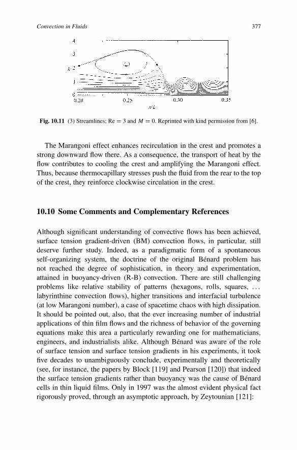
Convection in Fluids 377
Fig. 10.11 (3) Streamlines; Re = 3 and M = 0. Reprinted with kind permission from [6].
The Marangoni effect enhances recirculation in the crest and promotes astrong downward flow there. As a consequence, the transport of heat by theflow contributes to cooling the crest and amplifying the Marangoni effect.Thus, because thermocapillary stresses push the fluid from the rear to the topof the crest, they reinforce clockwise circulation in the crest.
10.10 Some Comments and Complementary References
Although significant understanding of convective flows has been achieved,surface tension gradient-driven (BM) convection flows, in particular, stilldeserve further study. Indeed, as a paradigmatic form of a spontaneousself-organizing system, the doctrine of the original Bénard problem hasnot reached the degree of sophistication, in theory and experimentation,attained in buoyancy-driven (R-B) convection. There are still challengingproblems like relative stability of patterns (hexagons, rolls, squares, . . .labyrinthine convection flows), higher transitions and interfacial turbulence(at low Marangoni number), a case of spacetime chaos with high dissipation.It should be pointed out, also, that the ever increasing number of industrialapplications of thin film flows and the richness of behavior of the governingequations make this area a particularly rewarding one for mathematicians,engineers, and industrialists alike. Although Bénard was aware of the roleof surface tension and surface tension gradients in his experiments, it tookfive decades to unambiguously conclude, experimentally and theoretically(see, for instance, the papers by Block [119] and Pearson [120]) that indeedthe surface tension gradients rather than buoyancy was the cause of Bénardcells in thin liquid films. Only in 1997 was the almost evident physical factrigorously proved, through an asymptotic approach, by Zeytounian [121]:

378 Miscellaneous: Various Convection Model Problems
. . . Either buoyancy is taken into account and in this case the free-surface deformation effect is negligible and we have the possibilityto take only partially into account the Marangoni effect, or this free-surface deformation effect is taken into account and in this case buoy-ancy does not play a significant rôle in the Bénard–Marangoni full ther-mocapillary problem.
It seems that the first author to explain (in a simple linear case) the effectof the surface tension gradients on Bénard convection was Pearson [120].The review article by Bragard and Velarde [122] has provided salient find-ings, old and recent, about Bénard convection flows in a liquid layer, heatedfrom below, and open to the ambient air. The Myers [123] paper is a reviewof work on thin films when (high) surface tension is a driving mechanism.Its aim is to highlight the substantial amount of literature dealing with rele-vant physical models and also analytic work on the resultant equations. Thepaper (in two parts) by Ida and Miksis [124] considers also the dynamicsof a general 3D thin film subject to van der Waals forces (which plays anessential role for ‘ultra-thin’ films), surface tension, and surfactants. Usingan asymptotic analysis based upon the thinness of the film with respect toits lateral extent, evolution equations for the leading-order film thicknesses,tangential velocities, and surfactant concentrations have been obtained. Thescaling was chosen by the above authors such that the surface tension effectsoccur at leading order in the dynamical model of the thin film. Note that theanalysis applies to the breaking of a thin liquid film off of a stable centersur-face. Unfortunately, the model equations, as presented, form a complicatedset of evolution equations and cannot be solved until the centersurface isprescribed. In part II of their work, Ida and Miksis [124] consider a seriesof special centersurfaces and in each case consider linear stability and solvethe resulting nonlinear equations numerically. In particular, it is shown thatincreasing surface tension is stabilizing, while increasing the effects of vander Waals forces is destabilizing; the effects of surfactants, although irrel-evant in determination of neutral stability curves, is stabilizing; the resultsobtained by solving the full evolution equations numerically agreed with thestability results obtained analytically. A weakly nonlinear analysis of cou-pled surface-tension and gravitational-driven instability in thin fluid layer(but, again, with a flat upper, free surface) is presented in [125]. In a weaklynonlinear analysis, it is sufficient to take into acount the modes that are crit-ical at the linear threshold and as a consequence for the critical modes. Inthe Parmentier et al. paper, a system of three coupled Ginzburg–Landau typeequations for the three amplitudes A1, A2, A3 is derived:

Convection in Fluids 379
τ∂Ai
∂t= εAi + aA∗
jA∗k − bAi[|Aj |2 + |Ak|2] − cAi |Ai |2 (10.39)
with i = 1 and j = 2, k = 3; i = 2 and j = 3, k = 1; i = 3 andj = 1, k = 2, wherein the coefficients τ , a, b and c depend generally onthe Prandtl and the Biot number and also on the ratio α (the percentage ofbuoyancy effect with regard to thermocapillary effect −α = 0 correspondsto pure thermocapillarity and α = 1 to pure buoyancy). The relative distancefrom the threshold is
ε = 1 − λ
λcwith λ = Ra
Ra0+ Ma
Ma0, (10.40)
where k is the wave number, and λc is related to the critical wave numberkc; Ra0 is the critical Rayleigh number for pure buoyancy and Ma0 is thecritical Marangoni number for pure thermocapillarity. According to Parmen-tier et al., when buoyancy is the single responsibility of the convection, onlyrolls will be observed. As soon as capillary effects are, however, observedit appears that a hexagonal structure is preferred at the linear threshold. Themore the thermocapillary forces are dominant with respect to the buoyancyforces, the larger the size of the region where hexagons are stable. It is shownthat the direction of the motion inside the hexagons is directly linked to thevalue of the Prandtl number and for Pr > 0.23, the fluid moves upward atthe center of the hexagons, in accordance with experiments. A subcriticalregion where hexagons are stable has also been displayed by these authors.The region is the largest when buoyancy does not act and in this case, thevalue found for the subcritical parameter is in excellent agrement with directnumerical simulation performed by Thess and Orszag [126]. But, all theseabove results correspond (unfortunately) to the case when the upper, freesurface is flat.
A detailed analysis of system (10.39) can be found in [127–129]. Instabil-ity of a liquid hanging below a solid ceiling (the so-called Rayleigh–Taylor(R–T) instability) has been considered by Limat in a short note [130] ac-cording to a lubrication equation derived in Kopbosynov and Pukhnachev(in 1986). He discussed the influence of the initial thickness on the R–T in-stability and the results are summarized by a diagram giving the differentpossible regimes. This diagram allows one to predict two different thick-ness dependencies that are selected by the physical properties of the liquid.For the vertical film, the review paper by Chang [131] gives an excellentsurvey concerning mostly the various transition regimes on an, isothermal,free-falling vertical film. For an extension of this review, see Chang and De-mekhin’s survey, [132], but note that in both these review papers, discussion

380 Miscellaneous: Various Convection Model Problems
of the Marangoni effect is absent. Nonlinear dynamics and breakup of free-surface flows is reviewed in the paper by Eggers [133]. This film rupture isalso considered by Ida and Miksis [134], who considered the dynamics of alamella in a capillary tube as well [135]. As papers concerning thin films ona rotating disk, we mention those by Sisoev and Shkadov, but again for theisothermal case.
Nonlinear evolution of waves on a vertically falling film (but unfortu-nately, without the Marangoni effect) is considered by Chang et al. [137].
In the above cited paper by Thess and Orszag [126], devoted to the limit ofthe infinite Prandtl number, the case of a high Marangoni number is also con-sidered. These authors note that ‘the kinematically possible velocity fieldscan have remarkable complexity when Ma � 1’, and it is a challengingproblem for future studies to understand Bénard–Marangoni convection inthe limit Ma → ∞.
Viscous thermocapillary convection at high Marangoni numbers is alsoconsidered by Cowley and Davis [138], where a boundary-layer analysis isperformed that is valid for large Ma and Pr. In the paper by Nepomnyaschyand Velarde [139], a dissipation-modified Boussinesq-like system of equa-tions governing 3D long wavelength Marangoni–Bénard oscillatory convec-tion in a shallow layer heated from the air side is presented. In this paper,solitary waves and their oblique and head-on interaction are also considered.Marangoni convection and instabilities in liquid mixtures with Soret effects(the inclusion of the so-called ‘Soret effect’ means that the mass flux is thesum of temperature and concentration gradients, but usually the so-calledDufour effect, by which the concentration gradient would contribute to theheat flux, is ignored) is considered by Joo [140] and more recently by Berg-eron et al. [141].
In Oron and Rosenau, [142], the authors show that the quadraticMarangoni instability enables an existence of new stable steady states whichin variance with the conventional Marangoni induced patterns, are continu-ous and do not rupture. It is interesting to note that the inherently unstableviscous liquid film flow down a vertical plate can be stabilized by oscillatingthe plate at appropriate amplitudes and frequencies, although the stabiliza-tion is obtainable only over a relatively small range of Re. The onset of steadyMarangoni convection, in a spherical shell of fluid with an outer free surfacesurrounding a rigid sphere, is analyzed by Wilson [143] using a combina-tion of analytical and numerical techniques. In a doctoral thesis by Vince[144], the propagative waves in convection systems subject to surface ten-sion effects are studied very accurately and a dynamical systems approach is

Convection in Fluids 381
also used, in particularly via amplitude equations à la Ginsburg–Landau (seeabove equations (10.39)).
An interesting and well-documented overview concerning drops, liquidlayers and the Marangoni effect is the paper by Velarde [145]. Spatio-temporal instability in free ultra-thin films is considered by Shugai andYakubenko [146]. The analysis shows that even in the linear approximation,the long-range intermolecular force strongly affects the evolution of initiallylocalized disturbances, but linear theory always overestimates the film lifetime, due to the explosive nonlinear growth of disturbances at later stages ofevolution. The IUTAM Symposium Proceedings (held in Haifa, Israel, 17–21March 1997) [147] concerned ‘Non-Linear Singularities in Deformation andFlow’. Various papers are related to interfacial effects in fluids and also withcapillary breakup and instabilities. In [148], RB convection and turbulenceis considered in liquid helium. The survey paper by Schechter et al. [149] isdevoted to the ‘two-component Bénard problem’. In [150] an infinite Prandtlnumber numerical similation in thermal convection is treated. The paper byChristov and Velarde [151] is an extension of the preceding paper [118]. Inthe special double issue of the Journal of Engineering Mathematics [152],the reader can find various papers devoted to the ‘dynamics of thin liquidfilm’. In [153] the Marangoni convection in a differentially heated binarymixture is studied numerically by continuation, the fluid being subject to theSoret effect. In a recent paper [154], the effects of surfactants on the forma-tion and evolution of capillary waves is considered numerically. The paperby Thual [155] is devoted to ‘zero-Prandtl-number convection’; indeed, thePrandtl = 0 convection is a singular problem considered, in particular, intheoretical fluid dynamics.
In another recent paper [156], a set of lubrication models for the thinfilm flow of incompressible fluids on solid substrates is derived and stud-ied. The models are obtained as asymptotic limits of the NS equations withthe Navier-slip boundary condition for different orders of magnitude for theslip-length parameter.
The recent very interesting, but rather ‘unusual’ book by de Gennes etal. [157] will enable the reader to understand in simple terms some mun-dane questions affecting our daily lives, questions that have often come tothe fore during our many interactions with industry (capillarity and wettingphenomena, drops, bubles, pearles and waves). The strategy in this book isto ‘sacrifice scientific rigor’ by an ‘impressionistic’ approach based on morequalitative arguments, which make it possible to grasp things more clearlyand to dream up novel situations!

382 Miscellaneous: Various Convection Model Problems
The recent book by Nepomnyaschy et al. [158], is devoted to ‘InterfacialConvection in Multilayer Systems’. It is unavoidable (see, the review by T.P.Witelski, Duke University, in SIAM Review) that this book has some overlapwith some of the authors’ previous books [159, 160] relative to ‘NonlinearDynamics of Surface-Tension-Driven Instabilities’ and ‘Interfacial Phenom-ena and Convection’. However, it is clear that this new book represents asignificant advance with more depth of analysis and a greatly extended setof models given in a systematic presentation.
The stability of an evaporating thin liquid film is considered (and recon-sidered) in a recent paper [161]. The paper [162] is devoted to ‘vorticity, freesurface and surfactants’. A few-mode Galerkin truncation is used in [163] toset up Lorenz models for convection in rotating binary mixtures. The work[164] develops a boundary-layer model for the thermocapillary feedbackmechanism that can occur in material processes, in the limit where convec-tion dominates heat transport but the Prandtl number is small. In [165] theRB convection with a temperature-dependent viscosity is considered from anasymptotic point of view and in [166] the temperature-dependent viscosityis also considered in the stability of a vertical natural convection boundarylayer. A systematic description of Marangoni convection in a rotating sys-tem is considered in [167]; a long-wave equation is derived, and numericalresults are discussed. In the recent paper [168], linear stability of a rotat-ing fluid-saturated porous layer heated from below and cooled from aboveis studied, when the fluid and solid phases are not in local thermal equilib-rium. A route to chaos in porous-medium thermal convection is considered in[169]. Surface-tension-driven Bénard convection in low-Prandtl-number flu-ids is studied in [170] by means of direct numerical simulations. In anotherrecent paper [171], Marangoni flow around chemical fronts traveling in thinsolution layers is considered, and influence of the liquid depth is numericallyanalyzed. A quantitative description of the combined action of anticonvectiveand thermocapillary mechanisms of instability is given in [172]. The onsetof multicellular convection in a shallow laterally heated cavity is studied in[173]. An asymptotic model of the mobile interface between two liquids in athin porous stratum is investigated in [174]. In [175], Grossmann and Lohsepropose a unified theory for ‘scaling’ in thermal convection. The film rupturein the diffusive interface model coupled to hydrodynamics is considered in[176] by Thiele et al.
As a ‘complement’ to the books [159, 160] published in 2001 and 2002,we mention the book [177], published in 2003, by Birikh et al., relative to‘Liquid Interfacial Phenomena – Oscillations and Instability’. Falling filmsand the Marangoni effect are considerd in [178] by Shkadov et al. The case

Convection in Fluids 383
of large Péclet numbers for a reactive falling film is considered in [179] byTrevelyan and Kalliadasis.
In 2005, Mutabazi et al. [180] published an ‘Henri Bénard Centenary Re-view’ concerning ‘dynamics of spatiotemporal structures’.
Scheid et al. [181] revisited the validity domain of the Benney equationin a case involving the Marangoni effect. The square patterns in rotating RBconvection are considered in [182] by Sánchez-Álvarez et al., and in [183]Sultan et al. considered the diffusion of the vapor and Marangoni instabilitiesin a problem relative to evaporation of a thin film. Traveling circular waves inaxisymmetric rotating convection have been investigated in [184] by Lopezet al.
Now, we mention some more recent papers (2007) by: Lopez etal. (‘Onset of convection in a moderate aspect-ratio rotating cylin-der: Eckhaus–Benjamin–Feir instability’) [185], Nepomnyashchy andSimanovskii (‘Marangoni instability in ultrathin two layer film’) [186],Merkt et al. (‘Short- and long evolution, in the long-wave theory of boundedtwo-layer films with a free liquid-liquid interface’) [187], Pereira et al. (‘Dy-namics of a horizontal thin liquid film in the presence of reactive surfac-tants’) [188] and Scheel (‘The amplitude equation for rotating RB convec-tion’) [189].
Finally, as papers published in 2008, I mention, among others, the pa-pers by: Sadiq and Usha (‘Thin Newtonian film flow down a porous in-clined plane: Stability analysis’) [190], Marques and Lopez (‘Influence ofwall modes on the onset of bulk convection in a rotating cylinder’) [191],Busse (‘Asymptotic theory of wall-attached convection in a horizontal fluidlayer with a vertical magnetic field’) [192], Dietze et al. (‘Investigation ofthe backflow phenomenon in falling films’) [193].
In an ‘Epilogue’ to conclude the present book, I should like to stress againthat, after working on it for two years, and after an attentive and careful finalre-reading of my typescript, I am yet more convinced that:
There is no better way for the derivation of significant model equationsthan rational analysis and asymptotic modelling.
A complete, consistent, rational modelling of the various convection phe-nomena in fluids is a long way in the future, but Chapter 8 in this bookshows that, concerning the Bénard, heated from below, convection problem,when we take into account three main effects (buoyancy, free-surface defor-mation and viscous dissipation) in starting fluid-dynamics formulation via arational approach, we have the possibility to derive three consistent, leading-

384 Miscellaneous: Various Convection Model Problems
order, approximate models; and more, if this is necessary we have at hands amethod for derivation of an associated, consistent, second-order model!
It is clear that, at the present time, an essential gap still exists between fluiddynamics modelling and numerical simulation; often the results of compu-tations (which are often ‘fascinating’) do not correspond, satisfactorily, toexperimental results! Rarely in publications do we see the theoretical treat-ment of a ‘full’ fluid film problem directly inspired from the technology. Forme, one reason is that, in starting physical problems, initial conditions areposed that obviously influence the formation and evolution (in time) of thefilm flow; thus the approximate models used for the numerical computationare not valid close to initial time. Further, with an ad hoc approach, often themodel used by the numericians is non-consistent, i.e., not well balanced!
In this book I have been highly selective in my choice of topics and inmany cases this choice of topics for rational analysis and asymptotic mod-elling has been based on my own interest and judgement. In fact, the mainpurpose of this book is only to give a fluid mechanics description of a certainclass of convection phenomena. To that extent the text is a personal expres-sion of my view of the subject.
References
1. B. Straughan, The Energy Method, Stability, and Nonlinear Convection, second edition.Applied Mathematical Sciences, Vol. 91, Springer-Verlag, New York, 2004.
2. K. Jöhnk and B. Svendsen, A thermodynamic formulation of the equations of motionand buoyancy frequency for Earth’s fluid outer core. Continuum Mech. Thermodyn. 8,75–101, 1996.
3. R.Kh. Zeytounian, The Bénard–Marangoni thermocapillary-instability problem. Phys.Uspekhi 41, 241–267, 1998
4. S. Kalliadasis, E.A. Demekhin, C. Ruyer-Quil and M.G. Velarde, J. Fluid Mech. 492,303–338, 2003.
5. C. Ruyer-Quil, B. Scheid, S. Kalliadasis, M.G. Velarde and R.Kh. Zeytounian, J. FluidMech. 538, 199–222, 2005.
6. B. Scheid, C. Ruyer-Quil, S. Kalliadasis, M.G. Velarde and R.Kh. Zeytounian, J. FluidMech. 538, 223–244, 2005.
7. A.A. Golovin, A.A. Nepommyaaschy and L.M. Pismen, Phys. Fluids 6(1), 35–48,1994.
8. D. Kashdan et al., Nonlinear waves and turbulence in Marangoni convection. Phys.Fluids 7(11), 2679–2685, 1995.
9. J.S. Turner, Multicomponent convection. Annu. Rev. Fluid Mech. 17, 11–44, 1985.10. P.H. Coullet and E.A. Spiegel, Amplitude equations for systems with competing insta-
bilities, J. Appl. Math. 43(4), 776–821, 1983.11. E. Knobloch, D.R. Moore, J. Toomre and N.O. Weiss, J. Fluid Mech. 166, 400–448,
1986.

Convection in Fluids 385
12. M.R.E. Proctor and N.O. Weiss, Normal forms and chaos in thermosolutal convection.Nonlinearity 3, 619–637, 1990.
13. R.Kh. Zeytounian, Asymptotic Modelling of Atmospheric Flows. Springer-Verlag,Berlin/Heidelberg 1990.
14. B.S. Dandapat and P.C. Ray, Int. J. Non-Linear Mech. 28(5), 489–501, 1993.15. C.I. Christov and M.G. Velarde, Dissipative solitons. Physica D 86, 323–347, 1995.16. A.Ye. Rednikov, M.G. Velarde, Yu.S. Ryazantsev, A.A. Nepomnyashchy and V.N. Kur-
dyumov, Cnoidal wave and solitary waves in a dissipation-modified Korteweg–de-Vriesequation. Acta Appl. Math. 39, 457–475, 1995.
17. D.R. Fearn and D.E. Loper, Compositional convection and stratification in the Earth’sfluid core. Nature 289, 393–394, 1981.
18. P. Melchior, The Physics of the Earth’s Core. Pergamon Press, Oxford, 1986.19. D.E. Smylie and A.M.K. Szeto, The dynamics of the Earth’s inner and outer cores. Rep.
Prog. Phys. 47, 855–906, 1984.20. F.D. Stacey, Applications of thermodynamics to fundamental Earth physics. Geoph.
Surveys 3, 175–204, 1977.21. R.Kh. Zeytounian, Recent avances in asymptotic modelling of tangent atmospheric mo-
tions. Int. J. Engng. Sci. 23(11), 1239–1288, 1985.22. P.H. Roberts and A.M. Soward, Magnetohydrodynamics of the Earth’s core. Annu. Rev.
Fluid Mech. 4, 117–154, 1972.23. W.W. Wood, A note on the westward drift of the earth’s magnetic field. J. Fluid Mech.
82, 349–400, 1977.24. M. Grae Worster, Annu. Rev. Fluid Mech. 29, 91–122, 1997.25. D.W. Hughes and M.R.E. Proctor, Annu. Rev. Fluid Mech. 20, 187–223, 1988.26. G. Schubert, Annu. Rev. Fluid Mech. 24, 359–394, 1992.27. J.C. MacWilliams, Annu. Rev. Fluid Mech. 28, 215–248, 1996.28. R.W. Griffiths, Annu. Rev. Fluid Mech. 18, 59–89, 1986.29. T.E. Dowling, Annu. Rev. Fluid Mech. 27, 293–334, 1995.30. A. Oberbeck, Ann. Phys. Chem., Neue Folge 7, 271–292, 1879.31. E. Knobloch, Rotating convection: recent developments. Int. J. Engng. Sci. 36(11),
1421–1450, 1998.32. S. Chandrasekhar, Hydrodynamic and Hydromagnetic Stability. Oxford University
Press, 1961.33. P. Germain, Introduction à l’étude de l’aéromagnétodynamique. Cahiers de Physique
103, 98–128, 1959.34. R.Kh. Zeytounian, Sur la magnétodynamique des fluides pesants. J. Méc. Appl. Phys.
Techn. (PMTF) 2, 37–42, 1980.35. H. Grad, Mathematical problem in magneto-fluid dynamics and plasma physics. in Pro-
ceedings of the International Congress of Mathematics, Stockholm, pp. 560–563, 1962.36. R.Kh. Zeytounian, Invariants lagrangiens et intégrales premières en magnétodynamique
des fluides. Appl. Sci. Res. 32(6), 593–596, 1976.37. A.S. Monin, Weather Forecasting as a Problem in Physics. Translated from Russian by
Paul Superak. The MIT Press, Cambridge, MA, 1972.38. R.Kh. Zeytounian, La météorologie du point de vue du mécaniciens des fluides. Fluid
Dynam. Trans. 8, 289–352, 1976.39. S.K. Wilson, The effect of a uniform magnetic field on the onset of steady Marangoni
convection in a layer of conducting fluid with a prescribed heat flux at its lower bound-ary. Phys. Fluids 6(11), 3591–3600, 1994.
40. K. Zhang and G. Schubert, Magnethydrodynamics in rapidly rotating spherical systems.Annu. Rev. Fluid Mech. 32, 409–443, 2000.
386 Miscellaneous: Various Convection Model Problems
41. R. Rosensweig, Ferrohydrodynamics. Cambridge University Press, 1985.42. P. Roberts, Electrohydrodynamic convection. Quart. J. Mech. Appl. Math. 22, 211–220,
1969.43. L. Landau, E. Lifshitz and L. Pitaevskii, Electrodynamics of Continuous Media. Perga-
mon, London, 1984.44. R. Turnbull, Phys. Fluids 11, 2588–2603, 1968.45. B. Deo and A. Richardson, Generalized energy methods in electrohydrodynamic sta-
bility theory. J. Fluid Mech. 137, 131–151, 1983.46. M. Cowley and R. Rosensweig, J. Fluid Mech. 30, 671–688, 1967.47. A. Gailitis, J. Fluid Mech. 82, 401–413, 1977.48. D. Wollkind and J. Bdzil, Comments on chemical instabilities. Phys. Fluids 14, 1813–
1814, 1971.49. A. Morro and B. Straughan, Convective instabilities for reacting viscous flows far from
equilibrium. J. Non-Equilib. Thermodyn. 15, 139–150, 1990.50. L. Rongy and A. De Wit, J. Engng. Math. 59, 221–227, 2007.51. S. Lebovich and S. Paolucci, The instability of the ocean to Langmuir circulations. J.
Fluid Mech. 102, 141–167, 1981.52. F. Crisciani, F. Cvallini and R. Mosetti, Stability of analytical solutions of Stommel–
Veronis ocean circulation models. J. Phys. Oceanography 24, 155–158, 1994.53. J. Pedlosky, Ocean Circulation Theory. Springer, Berlin/Heidelberg, 1996.54. G. Veronis, J. Fluid Mech. 31, 113–139, 1968.55. R.Kh. Zeytounian, Meteorological Fluid Dynamics. Lecture Notes in Physics, Vol. m5,
Springer-Verlag, Berlin/Heidelberg, 1991.56. R.Kh. Zeytounian, Weather prediction as a problem in fluid dynamics (On the 100th
Birthday of I. A. Kibel). Izv. Russ. Acad. Sci. Atmosph. Oceanic Phys. 40(5), 593–605,2004.
57. A.S. Monin, Fundamentals of Geophysical Fluid Dynamics. Original Russian edition,Hydrometeo-Izdat, Leningrad, 1988 [English translation available].
58. G.I. Marchuk and A.S. Sarkisyan, Mathematical Modelling of Ocean Circulation. Orig-inal Russian edition. Nauka, Moscow, 1988 [English translation available, Springer-Verlag].
59. G. Küppers and D. Lortz, J. Fluid Mech. 35, 609, 1969.60. S. Wiggins, Introduction to Applied Dynamical Systems and Chaos. Springer, New
York, 1990.61. E. Bodenschatz, W. Pesch and G. Ahlers, Recent developments in Rayleigh–Bénard
convection. Annu. Rev. Fluid Mech. 32, 709–778, 2000.62. K.M.S. Bajaj, L. Jun, B. Naberhuis and G. Alhers, Phys. Rev. Lett. 81(4), 806–809,
1998.63. R.M. Clever and F.H. Busse, J. Fluid Mech. 81, 609–627, 1979.64. M. Fantz, R. Friedrich, M. Bestehorn and H. Haken, Physica D 61(1–4), 147–154,
1992.65. J.J. Niemela and R.J. Donnelly, Phys. Rev. Lett. 57(20), 2524–2527, 1986.66. Y. Ponty, T. Passy and P.L. Sulem, Phys. Rev. E 56(4), 62–78, 1997.67. Y. Tu and M.C. Cross, Phys. Rev. Lett. 69(17), 2215–2219 and 2515–2518, 1992.68. G. Malone and S. Rionero, Continuum Mech. Thermodyn. 9, 347–363, 1997.69. B. Straughan, Mathematical Aspects of Penetrative Convection. Longman Group UK,
Harlow, 1993.70. G. Veronis, Penetrative convection. Astrophys. J. 137, 641–663, 1963.71. R. Krishnamurti, Convection induced by selective absortion of radiation: A laboratory
model of conditional instability. Dynam. Atmosph. Oceans 27, 367–382, 1997.

Convection in Fluids 387
72. K. Ames and B. Straughan, Acta Mech. 85, 137–148, 1990.73. B. Cushman-Roisin, Fluid Dyn. 19, 61–91, 1982.74. R.A. Denton and I.R. Wood, J. Fluid Mech. 113, 1–21, 1981.75. A.J. Faller and R. Kaylor, J. Geophys. Res. 75, 521–530, 1970.76. J.H. George, R.D. Gunn and B. Straughan, Geophys. Astrophys Fluid Dyn. 46, 135–158,
1989.77. R.L. Jennings, Geophys. Astrophys Fluid Dyn. 56, 183–204, 1991.78. P. Machetel and D.A. Yen, J. Geophys. Res. (B) 94, 10609–10626, 1989.79. P.C. Matthews, J. Fluid Mech. 188, 571–583, 1988.80. D.R. Moore and N.O. Weiss, J. Fluid Mech. 61, 553–581, 1973.81. J.M. Strauss, Astrophys. J. 209, 179–189, 1976.82. J.P. Zhan, J. Toomre and J. Latour, J. Geophys. Astrophys Fluid Dyn. 22, 159–193,
1982.83. V.Ya. Shkadov, Wave flow regimes of a thin layer of viscous fluid subject to gravity.
Fluid Dyn. 2, 29–34, 1967 [English translation].84. S. Kalliadasis, A. Kiyashko and E.A. Demekhin, J. Fluid Mech. 475, 377–408, 2003.85. P.M.J. Trevelyan and S. Kalliadasis, J. Engng. Math. 50(2–3), 177–208, 2004.86. C. Ruyer-Quil and P. Manneville, Eur. Phys. J. B15, 357–369, 2000.87. C. Ruyer-Quil and P. Manneville, Phys. Fluids 14, 170–183, 2002.88. D. Gottlieb and S.A. Orzag, Numerical Analysis of Spectral Methods: Theory and Ap-
plication. SIAM, Philadelphia, PA, 172 pp., 1977.89. C. Ruyer-Quil and P. Manneville, Phys. Rev. Lett. 93, 199401, 2004.90. M. Takashima, J. Phys. Soc. Japan 50(8), 2745–2750 and 2751–2756, 1981.91. P. Kaloni and Z. Qiao, Continuum Mech. Thermodyn. 12, 185–194, 2000.92. D.D. Joseph, Stability of Fluid Motion, II. Springer-Verlag, Heidelberg, 1976.93. H.E. Hupper and D.E. Moore, Nonlinear double-diffusive convection. J. Fluid Mech.
78, 821–854, 1976.94. Y. Ogura and N.A. Phillips, Scale analysis of deep and shallow convection in the at-
mosphere. J. Atmosph. Sci. 19, 173–179, 1962.95. D.O. Gough, The anelastic approximation for thermal convection. J. Atmosph. Sci. 26,
448–456, May 1969.96. B.G. Higgins, Film flow on a rotating disk. Phys. Fluids 29, 3522, 1986.97. B.S. Dandapat and P.C. Ray, Film cooling on a rotating disk. Int. J. Non-Linear Mech.
25, 529, 1990.98. M. Van Dyke, Perturbation Methods in Fluid Mechanics. Academic Press, New York,
1964.99. A. Kitamura, Asymptotic solution for film flow on a rotating disk. Phys. Fluids 12(9),
2141–2144, 2000.100. B. Reisfeld, S.G. Bankoff and S.H. Davis, The dynamics and stability of thin liquid
films during spin coating. I. Films with constant rates of evaporation or absorption. J.Appl. Phys. 70, 52–58, 1991.
101. A.G. Emslie, F.J. Bonner and L.G. Peck, Flow of a viscous liquid on a rotating disk. J.Appl. Phys. 29, 858, 1958.
102. Ch. Bailly, Modelisation asymptotique et numérique de l’écoulement dû à des disquesen rotation. Thesis, Université des Sciences et Technologies de Lille, No. 1512, 160 pp.,April 1995. See also Publication IRMA, Lille 33(XV), XV–2, XV–14, 1993.
103. D.J. Needham and J.H. Merkin, The development of nonlinear waves on the surface ofa horizontal rotating thin liquid film. J. Fluid Mech. 184, 357–379, 1987.
104. J. Liu and J.P. Gollub, Solitary waves dynamics of film flows. Phys. Fluids 6(5), 1702–1712, May 1994.

388 Miscellaneous: Various Convection Model Problems
105. R.Kh. Zeytounian, Nonlinear long waves on water and solitons. Phys. Uspekhi 38(12),1333–1381, December 1995 [English translation from Russian].
106. P.L. Kapitza and S.P. Kapitza, Zh. Exper. Teor. Fiz. 19, 105, 1949.107. A. Pumir, P. Manneville and Y. Pomeau, J. Fluid Mech. 135, 27, 1983.108. H.-C. Chang, E.A. Demekhin and D.I.Kopelevich, J. Fluid Mech. 250, 433, 1993.109. D.J. Benney, Long waves on liquid film. J. Math. Phys. 45, 150, 1966.110. M.G. Velarde and A.Ye. Rednikov, Time-dependent Bénard–Marangoni instability and
waves. In Time-Dependent Nonlinear Convection, P.A. Tyvand (Ed.), Adv. Fluid Mech.Series. Computational Mechanics Publications, Southampton, Chapter 6, pp. 177–218,1998.
111. M.G. Velarde (Ed.), Physicochemical Hydrodynamics. Interfacial Phenomena. Plenum,New York, 1988.
112. A.N. Garazo and M.G. Velarde, Phys. Fluids A3, 2295–2300, 1991.113. A.L. Frenkel, Europhys. Lett. 18, 583, 1992.114. J. Liu, J.D. Paul and J.P. Gollub, J. Fluid Mech. 250, 69, 1993.115. S.P. Lin and O. Suryadevara, Solitary, periodic and chaotic waves in thin films. In:
Transactions of the 2nd Army Conference on Applied Mathematics and Computing,ARO Report 85-1, pp. 483–499, 1985.
116. V.I. Nekorkin and M.G. Velarde, Int. J. Bifurcation Chaos 4(5), 1135–1146, 1994.117. M.G. Velarde, V.I. Nekorkin and A.G. Maksimov, Int. J. Bifurcation Chaos 5(3), 831–
839, 1995.118. C.I. Christov and M.G. Velarde, Evolution and interactions of solitary waves (solitons)
in nonlinear dissipative systems. Phys. Scripta T55, 101–106, 1994.119. M.J. Block, Surface tension as the cause of Bénard cells and surface deformation in a
liquid film. Nature 178, 650–651, 1956.120. J.R.A. Pearson, On convection cells induced by surface tension. J. Fluid Mech. 4, 489–
500, 1958.121. R.Kh. Zeytounian, The Bénard–Marangoni thermocapillary instability problem: On the
role of the buoyancy. Int. J. Engng. Sci. 35(5), 455–466, 1997.122. J. Bragard and M.G. Velarde, Bénard convection flows. J. Non-Equilib. Thermodyn. 22,
1–19, 1997.123. T.G. Myers, Thin films with high surface tension. SIAM Rev. 40(3), 441–462. 1998.124. M.P. Ida and M.J. Miksis, The dynamics of thin films I: General theory, and II: Appli-
cations. SIAM J. Appl. Math. 58(2), 456–473 and 474–500 1998.125. P.M. Parmentier, V.C. Regnier and G. Lebon, Nonlinear analysis of coupled gravita-
tional and capillary thermoconvection in thin fluid layers. Phys. Rev. E 54(1), 411–423,1996.
126. A. Thess and S.A. Orszag, Surface-tension-driven Bénard convetion at infinite Prandtlnumber. J. Fluid Mech. 283, 201–230, 1995.
127. M.C.Cross, Phys. Fluids 23, 1727. 1980.128. M.C. Cross, Phys. Rev. A 25, 1065, 1982.129. M.C. Cross and P.C. Hohenberg, Pattern formation outside of equilibrium. Rev. Mod.
Phys. 65, 851, 1993.130. L. Limat, Instabilité d’un liquide suspendu sous un surplomb solide: Influence de
l’épaisseur de la couche. C.R. Acad. Sci. Paris, Sér, II 217, 563–568, 1993.131. H.-Ch. Chang, Wave evolution on a falling film. Annu. Rev. Fluid Mech. 26, 103–136,
1994.132. H.-Ch. Chang and E.A. Demekhin, Solitary wave formation and dynamics on falling
films. Adv. Appl. Mech. 32, 1–58, 1996.

Convection in Fluids 389
133. J. Eggers, Nonlinear dynamics and breakup of free-surface flows. Rev. Mod. Phys.69(3), 835–929, 1997.
134. M.P. Ida and M.J. Miksis, Thin film rupture. Appl. Math. Lett. 9(3), 35–40, 1996.135. M.P. Ida and M.J. Miksis, Dynamics of a lamella in a capillary tube. SIAM J. Appl.
Math. 55(1), 23–57, 1995.136. G.M. Sisoev and V.Ya. Shkadov, Flow stability of a film of viscous liquid on a rotating
disk. J. Eng. Physics 52, 671–674, 1987 [English edition, translated from Russian].137. H.-Ch. Chang, E.A. Demekhin and E.A. Kopelevich, Nonlinear evolution of waves on
a vertically falling film. J. Fluid Mech. 250, 433–480, 1993.138. S.J. Cowley and S.H. Davis, Viscous thermocapillary convection at high Marangoni
number. J. Fluid Mech. 135, 175–188, 1983.139. A.A. Nepomnyaschy and M.G. Velarde, Phys. Fluids 6(1), 187–198, 1994.140. S.W. Joo, Marangoni instabilities in liquid mixtures with Soret effects. J. Fluid Mech.
293, 127–145, 1995.141. A. Bergeron et al., Marangoni convection in binary mixtures with Soret effect. J. Fluid
Mech. 375, 143–177, 1998.142. A. Oron and Ph. Rosenau, On a nonlinear thermocapillary effect in thin liquid layers.
J. Fluid Mech. 273, 361–374, 1994.143. S.K. Wilson, The onset of steady Marangoni convection in a spherical geometry. J.
Engng. Math. 28, 427–445, 1994.144. J.-M. Vince, Ondes propagatives dans des systèmes convectifs soumis à des effets de
tension superficielle. Doctoral Thesis, University Paris 7, No, 345, 185 pp., 1994.145. M.G. Velarde, Drops, liquid layers and the Marangoni effect. Philos Trans. Roy. Soc.
London A 356, 829–844, 1998.146. G.A. Shugai, and P.A. Yakubenko, Spatio-temporal instability in free ultra-thin films.
Eur. J. Mech. B/Fluids 17(3), 371–384, 1998.147. D. Durban and J.R.A. Pearson, Non-linear Singularities in Deformation and Flow.
Kluwer Academic Publishers, Dordrecht, 1999.148. R.P. Behringer, Rayleigh–Bénard convection and turbulence in liquid helium, Part I.
Rev. Mod. Phys. 57(3), 657–687, 1985.149. R.S. Schechter, M.G. Velarde and J.K. Platten, The two-component Bénard problem.
Adv. Chem. Phys. 26, 265–301, 1974.150. A. Lenardic and L. Moresi, Phys. Fluids 15(2), 455–466, 2003.151. C.I. Christov and M.G. Velarde, Dissipative solitons. Physica D 86, 323–347, 1995.152. D.G. Crowdy, C.J. Lawrence and S.K. Wilson (Guest Editors), The Dynamics of Thin
Liquid Films. Special Issue of J. Engng. Math. 50(2–3), 341 pp., November 2004.153. A. Bergeron et al., Marangoni convection in binary mixture with Soret effect. J. Fluid
Mech. 375, 143–177, 1998.154. H.T. Ceniceros, Phys. Fluids 15(1), 245–256, 2003.155. O. Thual, Zero-Prandtl-number convection. J. Fluid Mech. 240, 229–258, 1992.156. A. Munch, B. Wagner and T.P. Witelski, Lubrication models with small to large slip
lengths. J. Engng. Math. 53, 359–383, 2005.157. P.-G. de Gennes, F. Brochard-Wyart and D. Quéré, Capillarity and Wetting Phenomena,
Drops, Bubbles, Pearls, Waves. Springer Science + Business Media, 2004.158. A. Nepomnyaschy, L. Simanovskii and J.C. Legros, Interfacial Convection in Multi-
layer Systems. Springer-Verlag, New York, 2006.159. P. Colinet, J.C. Legros and M.G. Velarde, Nonlinear Dynamics of Surface-Tension-
Driven Instabilities. Wiley/VCH Verlag, Berlin 2001.

390 Miscellaneous: Various Convection Model Problems
160. A. Nepomnyaschy, M.G. Velarde and P. Colinet, Interfacial Phenomena and Convec-tion. Monogr. Surv. Pure Appl. Math., Vol. 124, Chapman & Hall/CRC, Boca Raton,FL, 2002.
161. O.E. Shklyaev and E. Fried, Stability of an evaporating thin liquid film. J. Fluid Mech.584, 157–183, 2007.
162. T. Sarpkaya, Annu. Rev. Fluid Mech. 28, 83–128, 1996.163. J.K. Bhattacharjee, Convection in rotating binary mixtures. III. Galerkin models. Phys.
Fluids A1(12), 1938–1948, 1989.164. D. Canright and M. Huber, Phys. Fluids 14(9), 3272–3279, 2002.165. J. Severin and H. Herwig, Z. angew. Math. Phys. 50, 375–386, 1999.166. J.-Y. Jang and J.C. Mollendorf, Int. J. Engng Sci. 26(1), 1–12, 1988.167. A.M. Mancho, H. Riecke and F. Sain, Chaos 12(3), 706–718, 2002.168. M.S. Malashetty, M. Swamy and S. Kulkami, Phys. Fluids 19, 054102, 2007.169. S. Kimura, G. Schubert and J.M. Straus, Route to chaos in porous-medium thermal
convection. J. Fluid Mech. 166, 305–324, 1986.170. T. Boeck and A. Thess, Bénard–Marangoni convection at low Prandtl number. J. Fluid
Mech. 399, 251–275, 1999.171. L. Rongi, A. De Witt, J. Engng. Math. 59, 221–227, 2007.172. A. Nepomnyaschy and L. Simanovskii, Phys. Fluids 14(11), 3855–3867, 2002.173. P.G. Daniels, P.A. Blythe and P.G. Simpkins, Onset of multicellular convection in a
shallow laterary heated cavity. Proc. Roy. Soc. London A 411, 327–350, 1987.174. M. Panfilov and M. Buès, Asymptotic model of the mobile interface between two liq-
uids in a thin porous stratum. J. Fluid Mech. 473, 59–81, 2002.175. S. Grossmann and D. Lohse, J. Fluid Mech. 407, 27–56, 2000.176. U. Thiele, M.G. Velarde, K. Neuffer and Y. Pomeau, Phys. Rev. E 64, 031602, 2001.177. R.V. Birikh, V.A. Briskman, M.G. Velarde and J.C. Legros, Liquid Interfacial Phenom-
ena Oscillations and Instability. Marcel Dekker, New York, 2003.178. V.Y. Shkadov, M.G. Velarde and V.P. Shkadova, Phys. Rev. E 67, 056310, 2004.179. P.M.J. Trevelyan and S. Kalliadasis, Phys. Fluids 16 (11), 3191, 2004.180. I. Mutabazi, E. Guyon and J.E. Wesfreid (Eds.), Dynamics of Spatiotemporal Structures
– Henri Bérnard Centenary Review. Springer, 2005.181. B. Scheid, C. Ruyer-Quil, U. Thiele, O.A. Kabov, J.C. Legros and P. Colinet, J. Fluid
Mech. 527, 303, 2005.182. J.J. Sánchez-Álvarez, E. Serre, E. Crespo del Arco and F.H. Busse, Phys. Rev. E 72,
036307, 2005.183. E. Sultan, A. Boudaoud and M. Ben Amar, J. Fluid Mech. 543, 183, 2005.184. J.M. Lopez, A. Rubio and F. Marques, J. Fluid Mech. 569, 331, 2006.185. J.M. Lopez, F. Marques, I. Mercader and O. Batiste, J. Fluid Mech. 590, 187, 2007.186. A.A. Nepomnyashvhy and I.B. Simanovskii, Phys. Fluids 19, 122103, 2007.187. D. Merkt, A. Potosky, M. Bestehorn and U. Thiele, Phys. Fluids 17, 064104, 2007.188. A. Pereira, P.M.J. Trevelyan and S. Kalliadasis, Phys. Fluids 19, 112102, 2007.189. J.D. Scheel, Phys. Fluids 19, 104105, 2007.190. I.M.R. Sadiq and R. Usha, Phys. Fluids 20, 022105, 2008.191. F. Marques and J.M. Lopez, Phys. Fluids 20, 024109, 2008.192. F.H. Busse, Phys. Fluids 20, 024102, 2008.193. G.F. Dietze, A. Leefken and Kneer, J. Fluid Mech. 595, 435–459, 2008.

Subject Index
Aa remarquable, (2.27), relation; 39
dimensionless form, (2.30); 40, 88adjustment-transient behavior; 50–52adverse conduction temperature gradient; 10,
11, 137adverse conduction gradient with TA; 112alternative; 2, 198Alfvén (A) number; 333amplitude equations; 150, 152, 154, 160,162, 248–250, 351–352, 359anelastic equations; 359–363
hydro-static case; 363Zeytounian dissipative system; 362, 363
approximate law state, 39asymptotic modelling; 104–108atmospheric thermal convevtion; 277averaged evolution equations; 209, 238–240
linear system; 240averaged IBL approach; 345–349
Bbasic adverse temperature gradient; 11, 79Bénard cells; 57Bénard problem in unbounded atmosphere;
319Benney equation; 223, 224
discussion; 223–225Biconv = B(H); 13, 204Biconv = B(T ); 13BH-C equations; 284, 285Biot numbers; 11BM equations: 200–204, 272–274BM instability; 197, 240, 349
BM long-wave equations; 207model problem; 211–214
BM problem with θ ; 252–254BM upper free surface conditions; 202–204body, electric, force f; 336Bois and Kubicki approach; 309Boltzmann’s constant; 35Bond (Bd) number; 64, 65, 197boundary conditions; 6Boussinesq approximation; 6Boussinesq hydrostatic convection
equations; 284–286Boussinesq number; 8breeze pronlem; 279–281breeze simple mechanism; 286, 287
two simple problem; 286–292Brunt-Väisälä frequency; 318, 329
CCharle’s law; 35characteristic equation; 217characteristic velocity Uc; 210chemical convection; 338, 339coefficient of thermal expansion; 7, 37
of isothermalcompressibility, β; 34, 37,56
coefficient χ ; 34coefficient of thermal expansion for water;
38, 56combined thermocapillary-buoyancy
convection; 168, 169comments concerning some recent
references; 377–384competition between hexagonal and roll
391

392 Subject Index
patterns; 258–260complementary references; 378–383conduction basic state Biot number; 11, 89conduction state; 10, 56, 93, 94conduction temperature �(z′); 199conduction temperature θ(z′); 200constant temperature Td ; 11constitutive relations; 5constitutive theory; 52, 53continuum regime; 3, 9–14convection Biot number; 11convection down a free-falling vertical liquid
film; 219, 220convection equations in atmosphere; 315
a simple case; 316, 317convection in the Earth’s outer core, 327–331convection in rotating cylinder; 342, 343convection over a curved surface; 298–300
Noe approach; 300–304Coriolis parameter; 24Cp; 32, 36, 37crispation (capillary) number; 16, 17, 95critical Rayleigh number; 193curvilinear coordinates; 288, 289cutoff wave number; 217, 227, 235Cv ; 33, 36
DDavis (1987) approach; 12–14Davis (1987) upper condition; 14, 46deep convection; 174
equations; 175, 176formula for Ra; 181linear theory; 177–181
matrix of Dff
; 178rigorous results; 189–192route to chaos; 182–188
deep thermal convection with viscousdissipation; 271, 272
dimensionless conditions; 103dimensionless reduced pressure; 15, 77dimensionless reduced pressure πs(z
′); 66dimensionless temperature θ ; 8, 14, 46, 90dimensionless temperature θs(z
′); 65dimensionless free surface; 93dimensionless temperature �; 10, 47, 89,198dimensionalization; 62, 133–135dispersion relation; 227, 245, 247
dispersion relation for Pr �= 0; 247dispersive similarity parameter; 233dissipation number Di = ε Bo; 8, 65, 271
of the specific kinetic energy; 311divergence of u; 5dominant equation for u′; 100dominant equation for θ ; 101dominant equation for �; 113double limiting process for anelastic
convection; 361dynamical system; 228, 235, 244
EE(t); 166Earth’s outer core convection 327–331
values; 330, 331EHD; 336
body force f; 336energy equation; 31enthalpy; 37entropy production inequality; 52epilogue: 383, 384ε2/ �≡ K0 = O(1); 88equation for the deformation of the free
surface; 16, 140equation for the temperature; 36
of a liquid; 39equation of state; 4, 30–32, 37, 43, 44, 80equation of state relative to TA and pA; 113estimation for E(t); 167estimation for the temperatures difference,
�T ; 21equation for the specific energy; 5, 31equation for T (dS/dt); 32, 34equation for ush with a term θ2
sh; 81estimation for the thickness, d , of the liquid
layer; 18, 20, 21evolution equations; 37, 40expansible liquid; 4, 38expansibility parameter, ε; 7, 20expansibility parameter, ε′; 198
Ffactor which affect breeze; 305, 306Feigenbaum period duobling scenario; 184–186FHD; 338film falling down (geometry); 126film falling down an inclined plane; 126–128

Convection in Fluids 393
Fourier law; 5four significant convections; 15, 102, 103free falling vertical film; 219–223free surface equation; 9, 41, 43free surface upper dimensionless conditions;
106–108Froude (Frd ) number; 2, 7, 87Froude (FrAd ) number; 198function �∗(χ); 213function �∗(H); 221function (χ); 214function (H); 222function q(t, x); 221
GGalileo number, Ga; 87gas constant; 36geometry of the Bénard problem; 93geostrophy; 292, 293Gibbs energy; 52Golovin et al. interaction approach; 349–351gradient; 4Grashof (Gr) number; 7, 18, 20, 63, 285
Hheat capacity; 32, 33, 36, 40heat flux (Fl); 312heat flux Rayleigh (Rl) number; 312Hills and Roberts’ equations; 53, 54
limit process; 75second-order model equations; 76
Howard & Krishnamurti DS; 160hydrostatic limit process; 282
equations; 282, 283hydrostatic parameter; 24, 282
IIBL isothermal model; 238IBL non-isothermal model; 239, 345–349initial conditions; 49–52isothermal coefficient of compressibility; 34
Jjump condition for T ; 12jump condition for θ ; 14
KKapitza (T ) number; 128Kazhdan computations; 352–354
Ki = (RF l)2/3Ta−5/6 Pe−1 � 1; 312
Kibel (Ki) number; 24, 310kinematic condition, 43Knudsen number, 163K0; 99Kronecker delta tensor; 4KS equation; 225, 256KS energy equation; 228KS–KdV equation; 233
DS system, 244generalized; 245
LLandau equation; 230
constant; 231leading-order system; 123limiting process; 16, 18, 21 137, 207
à la Boussinesq; 8, 66, 71DC; 18incompressible; 21N-ADH; 341quasi-hydrostatic; 24
linearization; 97, 98, 114linearized upper condition for �′ at z′ = 1;
114linear deep thermal convection theory;
176–181liquid hanging below a solid ceiling; 130liquid Mach number; 17local coordinates; 341local in time model; 208, 366local Prandtl convection model; 278local steady thermal convection problem;
294, 295long-wave (λ) parameter; 118, 282Lorenz dynamical system; 152, 154
strange attractor; 155–157lower bound for d; 7low Re and Ma theory; 231–233LS equation; 248–250
transition to chaos, 250, 251lubrication equations; 215, 216lubrication, one-dimensional equation; 217,
256lubrication theory; 196
MMach (atmospheric) number; 25Mach (liquid) number; 17

394 Subject Index
magneto-hydrodynamics; 331–336first integrals; 334quasi-steady limit equations; 334static equilibrium approximation; 334
magnetic induction, B; 333main effects in Bénard problem; 85Marangoni (Ma) number; 10, 128, 247Marangoni problem for film falling
down; 127, 128Ma with TA; 111matching; 50, 208material motion; 3Maxwell equations; 337Maxwell relations; 4, 32,33
for Cp − Cv ; 4, 33mean curvature; 41, 45mechanical pressure; 5, 31meso-scale prediction, (M-SP); 341, 342MHD convective equations; 333MHD equations; 333middle deck; 296model convection problem; 315, 316
simple problem; 316, 317modified Ma and We; 95mountain slop wind (Zeytounian); 319–322multi-scale approach; 145
NN , N1, N2; 202N-ADH limit process; 341Navier–Stokes equations; 30new coordinates and functions; 205, 206Noe approach; 300–304Newton’s cooling law; 10, 12, 14, 42, 220nonlinear stability for the deep convection;
190–192NS equation for ω = rot u; 311NS-F equations,
expansible liquid; 40for the Bénard problem, 96, 97thermally perfect gas; 37
NS-F 2D equations; 120Nusselt (Nu) number; 310
OOberbeck–Boussinesq equations; 357O–B simplified equations; 357, 358ocean circulation; 340–342Ohm’s law; 337
oscillatory convection; 307
Pparameter Bo′; 113parameter δ; 205parameters, W , W∗ and M ; 210parameter R∗; 207parameter F 2; 210parameters M∗ and W∗∗; 215parameters for atmospheric convection; 24Pearson approach; 115–117Pearson parameter L; 91, 116Pearson upper condition for �; 48penetrative convection; 343, 344Pellew and Southwell results; 69, 70phenomenological features; 304–306Pomeau–Manneville scenario; 187, 188Prandtl (Pr) number; 7, 64 201
mountain slope problem; 278pressure, p = (1/3)Tij
Qquasi-hydrostatic dissipative (Q-HD)
equations; 282, 283quasi-hydrostatic limiting process; 24, 282
RRa = ε Ga; 104Ra < Ta5/4; 313rate of change of surface tension; 9rate of loss Q(T ); 115rate of strain (deformation) tensor; 5, 30rate of viscous dissipation �; 5ratio, Cp/Cv = γ ; 33rational analysis; 104–110rational analysis and asymptotic modelling;104Rayleigh dimensionless problem; 62–66
conditions, 61Rayleigh equation for θ ; 64Rayleigh linear problem; 68–70Rayleigh number 7, 59, 63Rayleigh problem quations; 60RB convection patterns; 141, 142RB equations; 138, 140RB problem; 134, 135
in rarefied gases; 163–165RB rigid-rigid problem, 67, 68
second-order problem; 72

Convection in Fluids 395
RB standard model problem; 165, 166RB thermal shallow convection; 266–270reduced regularized model; 348, 349relation between, Td − TA and Tw − Td ; 13,
46relation between thermocapillay and
buoyancy effects; 259relationship between M∗∗, We∗ and R∗; 246Reynolds (Re) number; 50, 117Reynolds (Red ) number; 205Reynolds (Reλ) number; 207rigorous mathematical results; 189Rossby (Ro) number; 24, 283rotating RB convection; 308, 342Ruelle–Takens scenario; 183
Ssecond-order boundary layer solution for
temperature; 317second-order model equations; 72, 100, 101second-order model equations for RB; 143,
144short-scale – long-scale interaction; 349
amplitudes equations; 350attracteurs; 352, 353DS system; 351–354
short time for adjustment problem; 50similarity relations; 8, 16, 25, 77, 136, 210similarity rule between χ and α2; 40simple conduction problem; 93simple equation of state ρ = ρ(T ); 6simple-hump solitary waves; 375slope wind local problem; 288–292solar convection; 339solitary waves phenomena; 369–377
from IBL model; 376, 377head-on collision of the dissipativesolitons; 375homoclinic trajectories; 374localized structures, 374phase space representation;profile of a dissipative solitary wave;two-hump; 375
specific energy; 5specific entropy equation; 32specific entropy for a perfect gas; 37specific volume; 31sphericity parameter; 24squared sound speed; 34
stability results for KS equation; 226–231starting equations and conditions; 95, 96Stokes relation; 5strange attractors; 155–157, 159, 160,
183–188and intermittency; 186, 187by period doubling; 185from torii; 184infuence of the deep parameter; 188
stratification parameter; 285streamlines over a mountain slope; 302stress tensor; 3, 5Stuart–Landau (LS) equation; 244sub-critical instability; 166, 167surface gradient; 41surface tension; 9, 42, 48
TTakashima results; 241–243Taylor (Ta) number; 307, 307temperature �S(z′); 113temperature parameter τ ; 25thermal conductivity; 10thermal wind equation; 311thermally perfect gas; 4, 35, 36thermocapillary effect; 42, 196
convection with temperature-dependentsurface tension; 272–274
thermodynamic pressure; 5thermodynamic relations; 31, 34, 35, 37thermosolutal convection; 354–359thickness (lower bound); 7thickness dBM; 20thin liquid film over a rotating disk; 364–369
analyze via a lubrication equation; 368,369inner (in time) problem; 366outer equations; 364
three main facets of Bénard convection; 265three significant cases; 15, 102triple deck view point; 292–297typical values of Pr; 88
Uultra-thin film; 109unit outward normal vector; 41, 45unit tangent vectors; 44, 45upper bound for d; 136upper free surface conditions, 41–49, 76, 78,

396 Subject Index
202–204, 273, 274along the free surface; 78for the temperature; 12–14, 22, 42, 46, 48,199for the temperature θ ; 108, 200
linearized; 241for the temperature �; 112, 199for the motionless conduction state; 22for the pressure difference; 41, 44, 76upper deck; 296, 297
Vvector of rotation of the Earth; 24viscous dissipative function; 5, 32, 61viscous lower deck equations; 295, 296
WWe at TA; 111Weber (We) number; 10Weber (We∗) relations; 246
ZZeytounian anelastic dissipative equations;
362, 363Zeytounian approach for averaged IBL non-isothermal equations; 345, 346Zeytounian thermal atmospheric convection
approach (mountain slope wind); 320–322Zeytounian thermal deep convection; 172
equations; 174, 175