convergence analysis of a quadratic upper bounded tv regularizer based blind deconvolution
TRANSCRIPT

Contents lists available at ScienceDirect
Signal Processing
Signal Processing 106 (2015) 174–183
http://d0165-16
n CorrE-m
India.
journal homepage: www.elsevier.com/locate/sigpro
Convergence analysis of a quadratic upper bounded TVregularizer based blind deconvolution
M.R. Renu n,1, Subhasis Chaudhuri, Rajbabu VelmuruganElectrical Engineering Department, Indian Institute of Technology Bombay, Mumbai 400076, India
a r t i c l e i n f o
Article history:Received 5 July 2013Received in revised form8 April 2014Accepted 20 June 2014Available online 23 July 2014
Keywords:Blind deconvolutionTotal variationMajorize–minimizeAlternate minimizationConvergence analysis
x.doi.org/10.1016/j.sigpro.2014.06.02984/& 2014 Elsevier B.V. All rights reserved.
esponding author. Tel.: þ91 22 25764439.ail addresses: [email protected] (M.R. Rentb.ac.in (S. Chaudhuri), [email protected] to ISJRP funding by DST (Ref: No.IN
a b s t r a c t
We provide a novel Fourier domain convergence analysis for blind deconvolution usingthe quadratic upper-bounded total variation (TV) as the regularizer. Though quadraticupper-bounded TV leads to a linear system in each step of the alternate minimization(AM) algorithm used, it is shift-variant, which makes Fourier domain analysis impossible.So we use an approximation which makes the system shift invariant at each iteration. Theresultant points of convergence are better – in the sense of reflecting the data – than thoseobtained using a quadratic regularizer. We analyze the error due to the approximationused to make the system shift invariant. This analysis provides an insight into how TVregularization works and why it is better than the quadratic smoothness regularizer.
& 2014 Elsevier B.V. All rights reserved.
1. Introduction
In blind deconvolution a sharp image has to be obtainedfrom a single noisy and blurred observation without theknowledge of the point spread function (PSF). The imageobservation model is assumed to be a linear shift invariant(LSI) system. The observed image gets corrupted due to noiseand blur. Conventional image restoration techniques assumethat the blur (PSF) is known, whereas in blind restoration thePSF is taken as an unknown quantity and it is estimatedalong with the original image.
Blind restoration is an ill-posed problem due to thepossibility of multiple solutions and due to the fact thatthe solution changes by a large amount when there is asmall perturbation in the input, due to noise. An ill-posedproblem is converted to a well-posed problem usingregularizers [1]. A regularizer is an additional term added
u),(R. Velmurugan).T/SWISS/P-13/2009),
to the cost function to enforce certain conditions on theacceptable solution, thereby reducing the solution space.Commonly used regularization terms are the H1-norm(quadratic) that enforces smoothness [2], TV norm [3,4]that enables solutions which preserve edges, and waveletdomain regularizer [5–7] which favors solutions withsparse wavelet transforms since natural images areclaimed to have a sparse wavelet expansion.
The problem of blind deconvolution is a well studiedone, as can be seen from the numerous papers in theimage processing literature. Despite this, results on realworld images with large image and PSF sizes are rarelysatisfactory [8,9]. This is either due to the fact that most ofthe iterative methods take a long time to converge to anacceptable solution or due to the fact that non-iterativemethods do not work for all types of images and PSFs.Most of the solutions given in the literature could beclassified as either iterative or non-iterative in nature.Non-iterative methods of deconvolution, proposed in[9,10] are limited in the sense that they could be appliedonly for images which have a specific spectrum or for PSFswhich follow Levi distribution. Iterative methods of blinddeconvolution are more common [2,3,11–15] and are

M.R. Renu et al. / Signal Processing 106 (2015) 174–183 175
based on iterative procedures like alternate minimizationor expectation maximization. Use of total variation as aregularizer for blind deconvolution is reported in [3,16].A variational approach to blind deconvolution is givenin [17]. Sroubek and Flusser [18] propose a blind deconvo-lution method in a multichannel framework, which isapplicable when multiple observations of a scene is avail-able. In [19] a novel algorithm for blind deconvolutionfrom a pair of differently exposed images is reported.Iterative methods do not assume any properties for theimage and use certain general constraints on the PSF, likepositivity and symmetry, and hence are applicable to awider variety of images and PSFs. While using iterativemethods it is necessary to check whether these methodsconverge to a useful solution.
Few papers in the literature address the convergence ofiterative methods for blind deconvolution. The work byChambolle and Lions [20] analyzes the minimizationprocess for the case where the PSF is known. Figueiredoand Bioucas-Dias [21] have studied the sufficiency condi-tions for convergence in deconvolving Poissonian images,with the PSF assumed to be known. For the blind decon-volution case, the work by Chan and Wong [22] analyzesthe convergence of alternate minimization method for theH1 norm. With a Gaussian approximation to the TVfunction, [17] shows that the blind deconvolution algo-rithm converges.
In this paper, we consider a quadratic approximation ofTV as the regularizer, unlike in [3] where the TV withoutany approximation is used as the image and PSF regular-izer. Since the image and the PSF are both unknown, bothvariables need regularization and TV may be used in boththe cases [3]. This leads to a cost function having threeterms – the quadratic data term and the total variations ofthe image and the PSF. The data term contains the productof the unknown image and the PSF, and TV is a nonlinearfunction which results in a cost function that is non-linearand non-convex. In order to arrive at an optimum solutionfor the image and the PSF, we use the alternate minimiza-tion (AM) method. In AM a solution is arrived at bykeeping one variable fixed and minimizing w.r.t. the othervariable, so that at each step the problem reduces to that ofa non-blind restoration. In [3], where TV is used asregularizer for both the unknowns, variational approachis used to solve the blind deconvolution problem. In a laterpaper by Chan and Wong [22], a convergence analysis foralternating minimization algorithm for blind deconvolu-tion is reported. But the convergence analysis is restrictedto only H1 norm as it could not be extended to the TVnorm. In the case of H1 norm, an analysis is feasible sincein each step of the AM iteration, the cost function isquadratic in nature, whereas for TV norm this is not true,which makes an analysis difficult.
In order to do the convergence analysis we modify thecost function by replacing the TV norm by its quadraticupper bound, following the work of Figueiredo et al. [23].In [23,24] the upper bounding is used, respectively,for denoising and deconvolution with a known PSF. Weuse the upper bounding for solving blind deconvolutionwhere the PSF is not known. Using the quadratic upperbound for TV makes the cost function at each step of AM
quadratic in nature, though the overall cost functionremains non-quadratic. With this modification, we provide aconvergence analysis for blind deconvolution using alternateminimization with TV as a regularizer. The convergenceanalysis is done in the transform domain. Though approx-imating TV by a quadratic function makes the solution processlinear at each iteration, the system to be solved is not shiftinvariant. So we make a further approximation at eachiteration to make the system shift invariant. The convergencepoints reached with these two approximations is better thanthe convergence points obtained when a quadratic smooth-ness regularizer is used. We obtain the error incurred due toapproximating the system as a shift invariant one. The erroranalysis gives an insight into the regularization process whenTV is used as regularizer.
2. Deconvolution framework
The image formation model used is
y ¼Hxþn; ð1Þ
where y and x are MN � 1 vectors obtained by lexicogra-phically (i.e. converting the matrix to a vector by columnwise or row wise ordering; we have used row wiseordering) ordering the M � N observed image y and theoriginal image x, respectively. The noise term n is a sampleof additive white Gaussian noise and H is the MN �MNconvolution matrix obtained from the point spread func-tion (PSF) h of size P � Q . The PSF matrix is assumed to beof much smaller size than the image. In most practicalcases, the PSF is non-negative and exhibits lateral or radialsymmetry. These properties of the PSF will be used asconstraints along with the constraint that PSF is normal-ized to unity to prevent any shift in the mean of the image.
The problem of blind deconvolution aims at recon-structing the original image x and the PSF h from the noisyobservation y. We propose to estimate x and h (PQ � 1vector formed by lexicographically ordering h) using aquadratic data term and a TV regularizer for both theimage and the PSF. The cost function is given as
Cðx;hÞ ¼ ‖y�Hx‖2þλxTVðxÞþλhTVðhÞ; ð2Þ
subject to the constraints
hðm;nÞ ¼ hð�m; �nÞ; hðm;nÞZ0 8m;nand ∑
m∑nhðm;nÞ ¼ 1;
which come from symmetry, positivity and mean invar-iance, respectively. λx and λh are the image and PSF regu-larization factors, respectively. Total variation of x, TVðxÞ isdefined as
TVðxÞ ¼∑i
ffiffiffiffiffiffiffiffiffiffiffiffiffiffiffiffiffiffiffiffiffiffiffiffiffiffiffiffiffiffiffiffiðΔh
i xÞ2þðΔvi xÞ2
q; ð3Þ
where Δihand Δi
vcorrespond to the horizontal and vertical
first order differences at each pixel location, i.e. Δhi x¼ xi�xj
and Δvi x¼ xi�xl where xj and xl are the neighbors to left and
above, respectively, of xi. TVðhÞ is defined similarly. It shouldbe noted that (2) is highly nonlinear and this makes theconvergence analysis difficult. Figueiredo et al. [23,24] have
M.R. Renu et al. / Signal Processing 106 (2015) 174–183176
proposed a quadratic upper bound for TV, which makes theregularization terms quadratic in nature at each step of theiterations. As we show later, adopting such an approximationenables us to do the convergence analysis. It will be shownthat the iterations converge to a much better result than theone achieved in [22].
The method proposed by Figueiredo [23,24], approximatesTVðxÞ by the quadratic upper bound QTV ðx; xðkÞÞ, where xðkÞ isthe value of x at the kth iteration. The basis of this upperbounding is the inequality [23],ffiffiffia
pr ffiffiffiffiffi
a1p þa�a1
2ffiffiffiffiffia1
p with a1ra; a; a140: ð4Þ
Using (4), (3) is approximated as
TV x� �
rQTV ðx; xðkÞÞ9∑i
λ2
ðΔhi xÞ2þðΔv
i xÞ2ffiffiffiffiffiffiffiffiffiffiffiffiffiffiffiffiffiffiffiffiffiffiffiffiffiffiffiffiffiffiffiffiffiffiffiffiffiffiffiffiðΔh
i xðkÞÞ2þðΔvi xðkÞÞ2
q þKðxðkÞÞ;
ð5Þwhere the term KðxðkÞÞ is independent of x and hence doesnot affect the optimization process as explained in Figueir-edo et al. [23]. We have included the regularization factorλ as a part of TV in (5). It may be noted that the R.H.S. of (5)is quadratic in nature. In matrix notation, (5) can bewritten as
QTV ðx; xðkÞÞ9x 0D0ΛðkÞDxþKðxðkÞÞ; ð6Þwhere D denotes the matrix which when operating on avector gives the first order horizontal and vertical differ-ence of the vector. D is defined as D¼ ½ðDhÞ0 ðDvÞ0�0, whereDh and Dv denote matrices such that Dhx and Dvx are thevectors of all horizontal and vertical first order differencesof the vector x, respectively. Periodic boundary condition isused for x as well as h, while computing the first orderdifference. ΛðkÞ is defined as
ΛðkÞ ¼ diagðW ðkÞ;W ðkÞÞ; ð7Þwhere diagðLÞ refers to a diagonal matrix with elements ofvector L as the diagonal and W ðkÞ is a vector whose ithelement is
wðkÞi ¼ λx 2
ffiffiffiffiffiffiffiffiffiffiffiffiffiffiffiffiffiffiffiffiffiffiffiffiffiffiffiffiffiffiffiffiffiffiffiffiffiffiffiffiðΔh
i xðkÞÞ2þðΔvi xðkÞÞ2
q� ��1
: ð8Þ
Using (6) for image and PSF, and neglecting terms thatdo not affect the optimization, the cost function getsmodified as
Ckðx;hÞ ¼ ‖y�Hx‖2þx 0D0ΛðkÞx Dxþh 0D0ΛðkÞ
h Dh: ð9Þ
It is proved in [23] that using the quadratic approxima-tion leads to the same optimum as when TVðxÞ is used. Thefunction in (9) is nonlinear in both h and x. In orderto solve for h and x, we use the alternate minimization(AM) method [2,3]. Alternate minimization is an iterativemethod to solve cost functions of the form (9), with eachiteration consisting of two steps. In each step, one of thevariables is fixed and the resulting cost function is solvedfor the other variable. The steps in the AM algorithm are asfollows:
1.
Start with the initial values x0 and h0. Typically x0 is theblurred and noisy observed image, and h0 is chosen as asymmetric, non-negative, and normalized matrix.
2. Estimate x k from (9)with h ¼ h0, and initial value ofx ¼ x k�1. Here k is the iteration number.k
3.
Estimate h from (9) with x ¼ x k as obtained in step 2and initial h ¼ hk�1.4.
Repeat step 2 and step 3 till convergence.While estimating x at the ðkþ1Þth iteration by keepingh fixed, the cost function is essentially
Cx ðxÞ9Cðx;hÞjh ¼ h ðkÞ
¼ ‖y�Hx‖2þx 0D0ΛðkÞx DxþK1ðhðkÞÞ; ð10Þ
where K1ðhðkÞÞ ¼ hðkÞ0D0Λðk�1Þh DhðkÞ is a constant w.r.t. x, and
hence does not affect the optimization. From (10), xðkþ1Þ isestimated. Similarly the cost function for h, given x, is
Ch ðhÞ9Cðx;hÞjx ¼ x ðkþ 1Þ
¼ ‖y�Xh‖2þh 0D0ΛðkÞh DhþK2ðxðkþ1ÞÞ; ð11Þ
where X is the convolution matrix corresponding to theimage x. We have used the commutative property ofcircular convolution to write Hx ¼ Xh. Similar to thatin (10), K2 depends only on x, which is a constant whenminimization is done w.r.t. h, and hence can be neglectedduring the optimization process. Minimizing (11), giveshðkþ1Þ. These two steps are repeated till convergence.
The cost functions that appear in the AM steps arequadratic, as seen from (10) and (11). Given h, we solve forx by equating the gradient of (10) (∇Cx ) w.r.t. x to zero.Similarly, by equating ∇Ch to zero, we solve for h. This gives
ðH0kHkþD0ΛðkÞ
x DÞx ¼H0ky; ð12Þ
ðX0kþ1Xkþ1þD0ΛðkÞ
h DÞh ¼ X0kþ1y; ð13Þ
where Hk and Xk are the convolution matrices correspondingto the PSF and the image at the kth iteration. Let xk and hk bethe estimated image and PSF, respectively, at the kth iterationof AM. As the AM iterations proceed it needsto be seen whether the sequences fxkjk¼ 0;1;…g andfhkjk¼ 0;1;…g converge to some value xn and hn such that‖y�Hnxn‖2 is minimum. In the next section, we do theconvergence analysis and show that with proper choice ofregularization parameters, the AM iterations do converge to anon-trivial solution.
3. Convergence analysis
For analysis purpose we have assumed circular con-volution, which is commutative in nature, i.e. Hx ¼ Xhwhere X is the convolution matrix corresponding to x. Thevector h is padded with zeros to make its size same as thatof x. It may be noted from (10) and (11) that the costfunction for estimating x for a given h or h for a given x isquadratic in nature. The nature of the joint cost function (2) is,however, not quadratic due to the first term which isreproduced here for convenience
‖y�Hx‖2 ¼ y0y�2y0Hxþx 0H0Hx: ð14Þ

M.R. Renu et al. / Signal Processing 106 (2015) 174–183 177
Similar to [22] the convergence analysis can be carriedout in the frequency domain, by taking the discrete Fouriertransform (DFT) of (12) and (13). H and X being convolu-tion matrices corresponding to circular convolution, areblock circulant with circulant blocks (BCCB) and arediagonalized by the DFT as indicated in (15) and (16). LetFn denote a Fourier transform matrix of size N � N. TheBCCB matrices H and X are of size MN �MN. Then,
H¼ ðFm � FnÞΛHðFm � FnÞn; ð15Þ
X ¼ ðFm � FnÞΛXðFm � FnÞn; ð16Þwhere � indicates the Kronecker product and ΛH is adiagonal matrix whose diagonal entries correspond to theFourier transform of h, i.e.,
diagðΛHÞ ¼ ðFm � FnÞh: ð17Þ
Similarly,
diagðΛXÞ ¼ ðFm � FnÞx: ð18Þ
Let Xðξx; ξyÞ and Hðξx; ξyÞ represent the DFT of X and H,respectively. Eqs. (17) and (18) give H and X , respectively.
Since D¼ ½Dh0 Dv0 �0,
D0ΛðkÞh Dh ¼Dh0ΛðkÞ
hhDhhþDv0ΛðkÞ
hvDvh; ð19Þ
D0ΛðkÞx Dx ¼Dh0ΛðkÞ
xhDhxþDv0ΛðkÞ
xv Dvx; ð20Þ
where Λhh ¼Λhv ¼ diagðW ðkÞÞ, with W as defined in (8) andevaluated for the PSF. Λxh and Λxv are defined similarly using
the W for the image. The terms Dh0ΛðkÞhhD
h and Dv0ΛðkÞhvD
v
in (19) are unfortunately not BCCB, but the matrices Dv andDh which correspond to convolution matrix of the differenceoperation are BCCB, and are diagonalized by Fm � Fn. SinceDh is the convolution matrix corresponding to the first orderhorizontal difference, there exists an equivalent convolutionmask given by h1 ¼ ½0 1 �1�. Similarly the convolution mask
for Dh0 is h2 ¼ ½�1 1 0�. The convolution masks associatedwith Dv and Dv0 are h3 ¼ h01 and h4 ¼ h02, respectively.
From a system perspective, the matrix Dh0ΛðkÞhhD
h oper-ating on the vector h is equivalent to two convolutions anda multiplication in spatial domain given by
Dh0ΛðkÞhhD
h � h2⊛ðWðm;nÞ � ðh1⊛hÞÞ; ð21Þ
where ⊛ denotes the convolution operation and Wðm;nÞ isthe matrix form ofW as defined in (8). Here the ‘�’ operationindicates point wise multiplication. This system is shown inFig. 1. It may be noted that due to the multiplication byWðm;nÞ, the system though linear is not shift invariant.Using (21), the Fourier transform of Dh0ΛðkÞ
hhDh given by
Fig. 1. Equivalent system representation of Dh0ΛðkÞhhD
h . The diagonal matrix Λhh gevariant.
Rhhðξx; ξyÞ is written as
Rhhðξx; ξyÞ ¼H2ðξx; ξyÞ½Wðξx;ξyÞ⊛ðH1ðξx; ξyÞHðξx;ξyÞÞ�;ð22Þ
where H1 and H2, respectively, denote the DFT of h1 and h2(all DFT's are of size MN �MN), and Wðξx; ξyÞ is the Fouriertransform of Wðm;nÞ. Using (19) and (22), for a general hand x, the Fourier transform of (13) is written as
jXkj2 �Hkþ1þH2ðW⊛ðH1 �Hkþ1ÞÞþH4ðW⊛ðH3 �Hkþ1ÞÞ ¼Xkþ1Y;ð23Þ
where H3 and H4 are the Fourier transforms of the masksh3 and h4, respectively.
From (23), due to the frequency domain convolutions inthe second and third terms, one cannot write an expres-sion for Hkþ1. This happens since the system correspond-ing to (21) though linear is not shift invariant. If the systemwere linear shift invariant (LSI), it would have beenpossible to write an expression for Hðkþ1Þ, which makesanalysis feasible. It can be seen that this system becomesLSI, if Wðm;nÞ is a constant. In order to make the analysisfeasible, we use the assumption that Wðm;nÞ is constantfor each of the AM iterations and varies as the iterationchanges. But the question arises as to what value should bechosen for the constant. The entries Wðm;nÞ at theðkþ1Þth iteration are essentially the inverses of the mag-nitude of the gradient at each pixel, and the AM iterationsforce the magnitude of the gradient to decrease after eachiteration. Since the magnitudes keep decreasing withiteration we choose the maximum magnitude as theconstant, which decreases as the iterations proceed. Cor-respondingly we take Wðm;nÞ as a constant matrix filledwith the minimum value of Wðm;nÞ denoted byminðWkðm;nÞÞ, with k indicating the kth iteration. Thismodifies the regularization factor as λkh ¼ λh minðWkðm;nÞÞ.Since Wkðm;nÞ is a function of the total variation of h, werepresent λh
kas a function of hk,
λkhðhkÞ ¼ λh minðWkðm;nÞÞ: ð24Þ
With this approximation, D0ΛhD term in (13) becomesλkhD
0D and D0D operating on a vector x gives
D0Dx ¼∑m∑nj∇xðm;nÞj2; ð25Þ
which has a Fourier transform given by
Rðξx; ξyÞ ¼ 4�2 cos2πξxM
�2 cos2πξyN
;
ξx ¼ 0…M�1; ξy ¼ 0…N�1: ð26Þ
ts reflected as the multiplication by Wðm;nÞ which makes the system shift
M.R. Renu et al. / Signal Processing 106 (2015) 174–183178
With this approximation, (23) can be rewritten as
Hkþ1ðξx; ξyÞ ¼Xkðξx; ξyÞYðξx; ξyÞ
jXkðξx; ξyÞj2þλkhðhkÞRðξx; ξyÞ; ð27Þ
where R is given in (26) and λkhðhkÞ is as given in (24).Similarly, the DFT of (13) is obtained as
Xkþ1ðξx; ξyÞ ¼Hkþ1ðξx; ξyÞYðξx; ξyÞ
jHkþ1ðξx; ξyÞj2þλkxðxkÞRðξx; ξyÞ; ð28Þ
with
λkxðxkÞ ¼ λx minðWkðm;nÞÞ: ð29Þ
The expressions for the DFT of X and H as given by (27)and (28) are similar to [22] except for the difference that
regularization factors λkxðxkÞ and λkhðhkÞ change with eachAM iteration.
The phase of the Fourier transform of the reconstructedimage is the same as the phase of the observed image,provided the iterations used the observed image as theinitial value of the image. Under this condition the phaseof the Fourier transform of the estimated PSF is zero. Sincethe proof is the same as in [22] it is not reproduced here.
3.1. Convergence points for the magnitudes
Let ukþ1 ¼ jXkþ1ðξx; ξyÞj, vkþ1 ¼ jHkþ1ðξx; ξyÞj, r¼Rðξx; ξyÞ,and z¼ jYðξx; ξyÞj. Using these in the magnitude of (27) and(28), we get
ukþ1 ¼vkz
v2kþλkxðxkÞr; ð30Þ
vkþ1 ¼ukþ1z
u2kþ1þλkhðhkÞr
: ð31Þ
Substituting (31) in (30), update equations for the image andthe PSF in the Fourier domain, becomes
ukþ1 ¼ukz2ðu2
kþλkhðhkÞrÞu2kz
2þλkxðxkÞrðu2kþλkhðhkÞrÞ2
; ð32Þ
vkþ1 ¼vkz2ðv2kþλkxðxkÞrÞ
v2kz2þλkhðhkÞrðv2kþλkxðxkÞrÞ2
: ð33Þ
The magnitude spectrum updates of PSF and image at eachiteration depend on the gradients in the spatial domain PSFand image, respectively, through the terms λhðhkÞ and λxðxkÞ.Once the fixed point is reached, u and v do not change furtherand hence the regularization factors also remain constant.It maybe noted that this is the main difference between usingthe approximated TV and the smoothness regularizer of [22].In [22], the regularization factors remain constant throughoutthe iteration and the fixed point depends on the tworegularization factors. In our analysis, both the regularizationfactors change depending on the signal (image/PSF) and reacha final value on which the fixed point depends.
From (32),
ukþ1 ¼ FðukÞ; ð34Þ
where FðukÞ is
F ukð Þ ¼ ukz2ðu2kþλhðhkÞrÞ
u2kz
2þλxðxkÞrðu2kþλhðhkÞrÞ2
: ð35Þ
At the fixed point FðuÞ ¼ u. Let λhf and λxf be the regular-ization factors corresponding to the PSF and the image,respectively, once the fixed points have been reached.Once the fixed point is reached, the scenario is similarto that in [22], hence the proof of convergence is notreproduced here. Instead, we highlight how the conver-gence points from our analysis differ from that of [22].From (35) the fixed points u1; u2 can be calculated as
u1 ¼ 0;
u2 ¼
ffiffiffiffiffiffiffiffiffiffiffiffiffiffiffiffiffiffiffiffiffiffiffiffiffiffiffiffiffiffiffiffiffiffiffiffiλhfλxf
sz�λhf r
vuut
For zrffiffiffiffiffiffiffiffiffiffiffiffiffiλhf λxf
qr, the fixed point u1 is reached, and for
z4ffiffiffiffiffiffiffiffiffiffiffiffiffiλhf λxf
qr, the fixed point u2 is reached provided the
initialization for the image is non-zero. Hence the conver-gence points for the magnitude are given by a lemmasimilar to that in [22].
Lemma 1. The magnitude spectra of the image and the PSFconverge to
MT ¼
ffiffiffiffiffiffiffiffiffiffiffiffiffiffiffiffiffiffiffiffiffiffiffiffiffiffiffiffiffiffiffiffiffiffiffiffiffiffiffiffiffiffiλhfλxf
sjYj�λhfR
vuut and
ffiffiffiffiffiffiffiffiλxfλhf
sMT ;
respectively, when jYj24λxf λhfR2, else they both convergeto zero.
The difference between the convergence points in [22]and those given by Lemma 1 is that in [22] the conver-gence points can be obtained directly without usingan iterative procedure whereas our analysis indicatesconvergence points that are reached once the iterationsconverge to the fixed point. But forcing the system to bespace invariant makes the magnitude of the estimatedimage and the PSF proportional to each other. In theerror analysis given in the next section we show thatwithout this approximation, a space varying regularizationis achieved.
A signal processing perspective of the convergenceprocess is as follows. At the kth iteration new values forthe image and the PSF are obtained based on which theregularization parameters λkxðxkÞ and λkhðhkÞ are calculated.The next iteration proceeds with these modified regular-ization parameters. Hence the quadratic upper boundedTV behaves like an adaptive regularizer. From the discus-sion in the previous section, it is seen that the values ofregularization parameters decide the quality of reproducedimages. Since in this case the regularization parametersare gradually adjusted to a value that depends on the totalvariation of the image and the PSF, convergence to a bettersolution is expected. It is seen from the experiments thatthe regularization parameters reduce and converge to avalue determined by the TV of the image and the PSFleading to an improved solution. This is expected since
M.R. Renu et al. / Signal Processing 106 (2015) 174–183 179
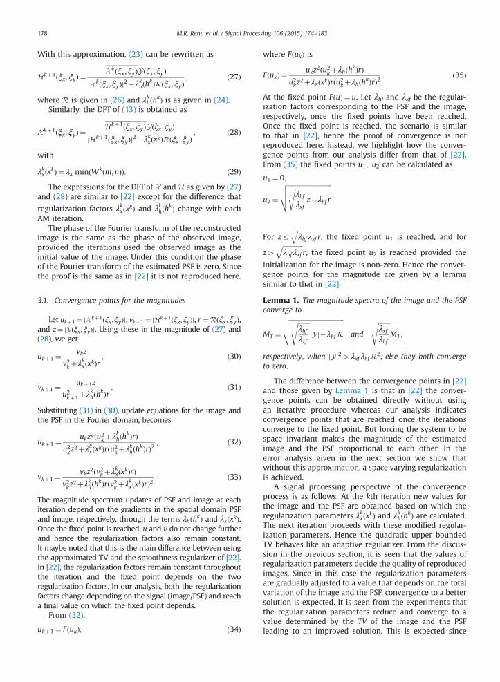
minimization of the TV norm leads to the reduction of theregularization factors at each iteration till the fixed point isreached, after which they remain constant. The productλkxλ
kh is shown in Fig. 2(d) and Fig. 3(d) does conform to this
statement.The update equations (27) and (28) are similar to that
of the Wiener filter [25], except that the proposed methodis a purely deterministic approach. Instead of a fixed filterfor restoring the image, the iterations converge to a filterwhich depends on the total variation of the image and thePSF. Hence the proposed approach may be thought of as aWiener filter that adapts to the image and PSF totalvariations to give an optimum solution. It may also benoted that the selection of the regularization factors showsa similarity to the step-size selection in gradient descentalgorithms, in the sense that too low or too high initialvalues of regularization factors lead to convergence to atrivial solution.
0 20 40 60 80 100 1200
5
10
15
20
25
30
35
40
iterations (k)
PS
NR
kk
Fig. 2. Deconvolution for 3�3 Gaussian mask, with zero noise. (a) Blurred imageof the product of regularization factors (λxλh) with iteration.
4. Analysis of error due to approximation
In the previous section, the Wðm;nÞ matrix wasapproximated to be a constant matrix so that the resultantsystem is LSI at each iteration. This leads to convergencepoints for the image and the PSF which have magnitudesrelated to each other. The error due to this approximationis analyzed in this section. Keeping the PSF constant, thecost in (9) reduces to
CðxÞ ¼ ‖y�Hx‖2þλxx 0D0ΛxDx: ð36Þ
The estimated solution x is the one which makes thegradient of (36) zero.
ðH0HþD0ΛDÞx ¼H0y: ð37Þ
The estimated solution is
x ¼ ðH0HþD0ΛDÞ�1H0y; ð38Þ
0 10 20 30 40 50 60 70 80 90 1000
1000
2000
3000
4000
5000
6000
iterations (k)
λ xλh
. (b) Deconvolved image. (c) Variation of PSNR with iteration. (d) Variation
0 5 10 15 20 25 30 35 400
5
10
15
20
25
30
iterations (k)
PS
NR
0 5 10 15 20 25 30 351
2
3
4
5
6
7
8
9
10
11
iterations (k)
λ xk λhk
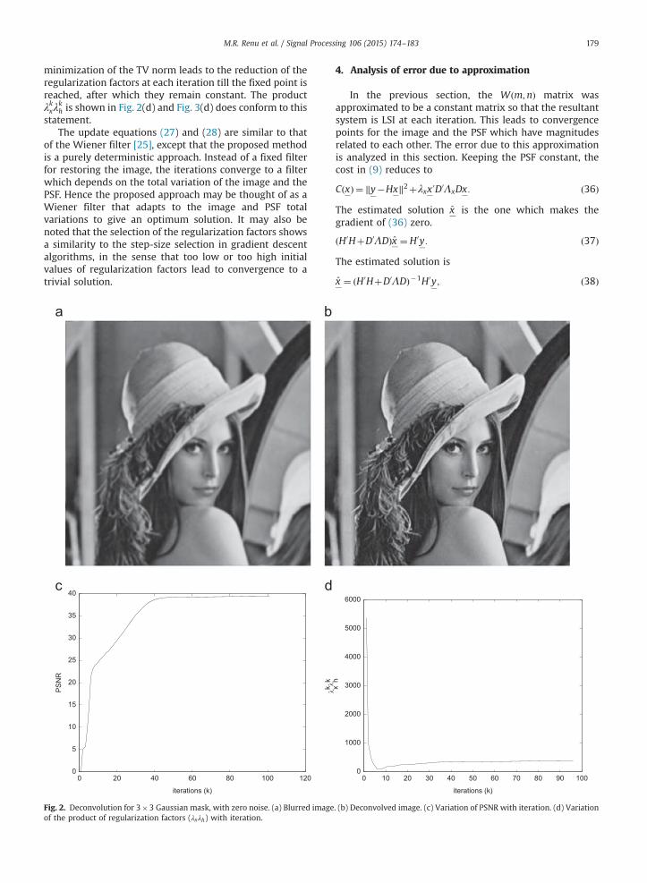
Fig. 3. Results of deblurring for a 5�5 mask, and noise variance 10. (a) Blurred and noisy input image. (b) Deblurring result with a constant approximationonWðm;nÞ, ringing is noticed and PSNR is improved by 2 dB. (c) Deblurring result with quadratic upper bound on TV, the PSNR improved by 3 dB. (d) Resultof deblurring for low value of regularization parameter for PSF regularizer, a trivial solution is obtained. (e) Variation of PSNR with iteration for theproposed method. (f) Variation of the product of the two regularization terms with iteration.
M.R. Renu et al. / Signal Processing 106 (2015) 174–183180
M.R. Renu et al. / Signal Processing 106 (2015) 174–183 181
provided the solution exists. The matrix inversion lemma(MIL)
ðAþBCEÞ�1 ¼ ðIþA�1BCEÞ�1A�1 ð39Þis used to expand the inverse term in (38). From (7) it isseen that Λ is a diagonal matrix with entries inverselyproportional to the magnitude of the gradient at each pixelposition. Λ is split into the sum of two diagonal matrices
Λ¼ΛminþΛres; ð40Þwhere Λmin is a diagonal matrix with all entries equal tothe minimum non-zero valued entry of Λ, and Λres is adiagonal matrix with diagonal entry as the difference indiagonals of Λ and Λmin. With this modification, x becomes
x ¼ ðH0HþD0ΛminDþD0ΛresDÞ�1H0y: ð41Þ
Since all the diagonal elements in Λmin have the samevalue (say λmin), D
0ΛminD¼ λminD0D. Applying MIL to (41),
with A¼H0HþλminD0D, B¼D0ΛresD, and C ¼ E¼ I,
x ¼ ½IþðH0HþλminD0DÞ�1D0ΛresD��1ðH0HþλminD
0D�1H0y;
ð42Þ
x ¼ ½IþP��1xs; ð43Þwhere P ¼ ðH0HþλminD
0DÞ�1D0ΛresD and xs ¼ ðH0HþλminD
0D�1H0y. From the expression for xs, it is seen thatthis component corresponds to the solution obtained witha smoothness regularizer as was done in [22]. If jPjo1,
½IþP��1 ¼ I�PþP2�P3þ⋯ ð44ÞIn the previous analysis given in Section 3, we approxi-mated the solution at each iteration to the smoothnesssolution, which amounts to keeping only the first term ofthe expansion in (44). Assuming that jPjo1 (we shall seelater how this condition is enforced), the estimated solu-tion can be written as
x ¼ xsþ ∑1
n ¼ 1ð�1ÞnPnxs: ð45Þ
The operator P is a combination of two operators:P2 ¼D0ΛresD, which extracts the high frequency component,being a derivative operator and P1 ¼ ðH0HþλminD
0D�1 whichdoes a regularized inverse on its argument. To understand theeffect of the operator P2, we split it as
D0ΛresD¼D0∑iΛi
minD; ð46Þ
where Λmini
is a diagonal matrix with the diagonal elementsgiven by
diagðΛiminÞ ¼minðdiagðΛi�1
res ÞÞ filled at the
non� zero locations of Λi�1res
diagðΛiresÞ ¼ diagðΛi�1
res Þ�minðdiagðΛiminÞÞ at the
non� zero locations of Λi�1res ; ð47Þ
where diagðAÞ, for a matrix A, is defined as the diagonal of thematrix A. The minð�Þ function returns the smallest non-zerovalue of the vector argument. The number of diagonalelements that are zero increases with i. Therefore,
P2x ¼∑iD0Λi
minDx ð48Þ
P2x ¼∑iλimin∑
jgj; ð49Þ
where gj is the negative of the gradient of x. So essentiallyP acting on the vector xs has the effect of adding morecomponents of higher frequency which are regularized by theP1 operator. We note that this is a spatially varying regulariza-tion. The spatial points with small gradients get regularizedmore since the points which survive for larger values of i arethose with small gradients and these points get regularized ateach value of i (the elements of Λres are essentially the inverseof magnitude of gradient at each pixel point). This is reason-able since the noise amplification would be less for points oflow gradients and hence it is feasible to take higher orderderivatives of such points. Each time, the P operator isused, regularized high frequency components are added, withthe Λmin
icontrolling noise amplification.
The condition jPjo1 requires γminðP1ÞγmaxðP2Þr1,where γminðP1Þ is the minimum eigenvalue of P1 andγmaxðP2Þ is the maximum eigenvalue of P2. The user hasto make sure that the condition jPjo1 is satisfied byappropriately selecting the regularization factors whichwould ensure that γminðP1ÞγmaxðP2Þr1. A similar analysiscan be done for the PSF estimation part. This analysis givesan insight into the operation of the TV regularizer. Theerror incurred by the approximation to make the systemshift invariant is that the high frequencies are not wellregularized, leading to a partial loss of high frequencyinformation, which is seen in the result section in Fig. 3(b).
5. Results and discussions
In this section we provide experimental results thatsubstantiate our analysis. To estimate both the image andthe PSF, we need to solve (12) and (13), respectively.Eq. (12) is evaluated using the conjugate gradient method.Since H in (12) is the convolution matrix, ðHk
0HkþD0ΛðkÞx DÞx
is easily calculated through convolution using the masksh1 and h2 for evaluating the second term. We first attemptto estimate the PSF from (13) using both constrainedand unconstrained methods, with constraints on h asmentioned in Section 1. For the constrained optimizationimplemented in MATLAB, running even on a quad proces-sor machine, the time taken for convergence and thememory requirements needed for specifying the con-straints become too high to be of any practical use forlarge PSF size. For large PSF sizes the problem is convertedto an unconstrained optimization by penalizing the costfunction to enforce the PSF symmetry and by projectingthe solution to ensure positivity and mean invariance. Theresults obtained are similar in both the cases, but thespeed of convergence is much better for the conjugategradient implementation.
For the constrained optimization case, the results ofdeconvolution obtained for a 3�3 mask are shown inFig. 2. In Fig. 2, the noise variance is zero, and the peaksignal to noise ratio (PSNR) of the restored image in thiscase is 39.3 dB which is a large improvement over thePSNR of the blurred input image (29 dB). The blurredand the deblurred images are shown in Fig. 2(a) and (b),respectively. Fig. 2(c) shows how the PSNR varies with

M.R. Renu et al. / Signal Processing 106 (2015) 174–183182
iterations, and Fig. 2(d) shows change in the product ofthe regularization parameters (λxλh) with iterations.It decreases initially and stabilizes at a value whichdepends on the total variation of the original image andthe PSF. It is this nature of variation that leads to a betterresult compared to quadratic smoothness regularizer. Themean square error between the estimated and the originalPSF is 4:54� 10�6.
Deconvolution in the presence of noise is acknowl-edged to be difficult. We show the performance of themethod against noise now. The results of deblurring for anoise variance of 10 is given in Fig. 3. The mask used hereis a Gaussian kernel of size 5�5 with a spread of 3. ThePSNR improvement obtained in this case is 3 dB. The meansquare error in the estimated PSF is 1:79� 10�5. Thusthere is a definite improvement but not as dramatic as inFig. 2. Fig. 3(a) shows the blurred and noisy image. Fig. 3(b)shows the reconstructed image with approximation onWðm;nÞ, in which the ringing effect due to spectrum beingforced to zero is visible. This may be compared withFig. 3(c), which shows the result of blind deconvolutionwith no approximation on Wðm;nÞ. In the latter case noringing is seen. It is seen that in the case where the noisevariance is non-zero, the estimated PSF could converge tothree different values depending on the initial value of thePSF regularization term (λh). If λh is small, the PSFconverges to impulse function and the estimated imageis the same as the original (Fig. 3(d)). If λh is large, the PSFconverges to an averaging mask, with total variation closeto zero, and reduces to an averaging filter. For an inter-mediate value of λh, which we determine empirically, thePSF converges to a value close to the original, with meansquare error of the order of 10�5.
In the implementation using conjugate gradient, whileestimating the PSF it is not computationally economical todo an optimization over a h of size same as the image size.So the gradient with respect to hðk; lÞ is evaluated using
‖y�Hx‖2 ¼∑m∑n
yðm;nÞ�∑k∑lhðk; lÞxðm�k;n� lÞ
!2
: ð50Þ
This reduces the advantage of conjugate gradient w.r.t.speed, but still performs much faster than the constrainedcase. The result for conjugate gradient is comparable tothat obtained using the constrained optimization, with theadded advantage that it is several orders of magnitudefaster than the constrained optimization case.
6. Conclusions
We have proposed the quadratic upper bounded TVfunction as the regularizer for both the image and the PSF,which gives the advantage of quadratic cost functions in theAM iterations, making the problem amenable for conver-gence analysis. We provide the convergence analysis, whichshows that with each iteration of the alternate minimiza-tion algorithm, the regularization factors gets modified,eventually leading to an acceptable solution. We alsoprovide an argument for why the TV norm performs betterthan the smoothness regularizer. In order to make Fourierdomain analysis feasible we approximate the system to be
linear shift invariant at each iteration. It is observed that theconvergence point of the magnitude of the image and thePSF thus obtained is related to each other. We also do ananalysis of the error introduced due to the approximation tomake the system LSI at each iteration. It is shown that bymaking the system LSI, the regularization for higher spatialfrequencies is lesser compared to the quadratic upper-bounded TV. From the analysis of the error term, it is seenthat the approximation cuts off the high frequency infor-mation leading to a quality degradation in the deconvolvedresult. The error analysis also shows that the TV regularizeressentially adds regularized high frequency components tothe smoothness based solution, leading to a better solutionthan the smoothness based one.
References
[1] A.N. Tikhonov, Solution of incorrectly formulated problems and theregularization method, Soviet Math. 4 (1963) 1035–1038.
[2] Y. You, M. Kaveh, A regularization approach to joint blur identifica-tion and image restoration, IEEE Trans. Image Process. 5 (3) (1996)416–428.
[3] T.F. Chan, C.K. Wong, Total variation blind deconvolution, IEEE Trans.Image Process. 7 (3) (1998) 370–375.
[4] L. Rudin, S. Osher, Total variation based image restoration with freelocal constraints, in: IEEE International Conference on Image Proces-sing, 1994. Proceedings. ICIP-94, vol. 1, 1994, pp. 31–35.
[5] M.A.T. Figueiredo, J.M. Bioucas-Dias, R.D. Nowak, Majorization–minimization algorithms for wavelet-based image restoration, IEEETrans. Image Process. 16 (12) (2007) 2980–2991.
[6] C. Vonesch, M. Unser, A fast multilevel algorithm for wavelet-regularized image restoration, IEEE Trans. Image Process. 18 (3)(2009) 509–523.
[7] R. Neelamani, H. Choi, R.G. Baraniuk, Wavelet-domain regularizeddeconvolution for ill-conditioned systems, in: ICIP (1), 1999,pp. 204–208.
[8] A. Levin, Y. Weiss, F. Durand, W.T. Freeman, Understanding andevaluating blind deconvolution algorithms, in: CVPR, IEEE, MiamiBeach, Florida, USA, 2009.
[9] A.S. Carasso, Direct blind deconvolution, SIAM J. Appl. Math. 61 (6)(2001) 1980–2007.
[10] V. Nourrit, B. Vohnsen, P. Artal, Blind deconvolution for high-resolution confocal scanning laser ophthalmoscopy, J. Opt. A: Pure.Appl. Opt. 7 (2005) 585–592.
[11] G.R. Ayers, J.C. Dainty, Iterative blind deconvolution method and itsapplications, Opt. Lett. 13 (7) (1988) 547–549.
[12] A.C. Likas, N.P. Galatsanos, A variational approach for blind imagedeconvolution, IEEE Trans. Signal Process. 52 (8) (2004) 2222–2232.
[13] A.K. Kastaggelos, K.T. Lay, Maximum likelihood blur identificationand image restoration using the EM algorithm, IEEE Trans. SignalProcess. 39 (3) (1991) 729–733.
[14] E.Y. Lam, J.W. Goodman, Iterative blind deconvolution in space andfrequency domains, in: Proceedings of SPIE, vol. 3650, 1999,pp. 70–77.
[15] P. Pankajakshan, B. Zhang, L. Blanc-Féraud, Z. Kam, J.-C. Olivo-Marin,J. Zerubia, Blind deconvolution for thin layered confocal imaging,Appl. Opt. 48 (22) (2009) 4437–4448.
[16] D. Babacan, R. Molina, A. Katsaggelos, Variational Bayesian blinddeconvolution using a total variation prior, IEEE Trans. ImageProcess. 18 (1) (2009) 12–26.
[17] R. Molina, J. Mateos, A. Katsaggelos, Blind deconvolution using avariational approach to parameter, image, and blur estimation, IEEETrans. Image Process. 15 (12) (2006) 3715–3727.
[18] F. Sroubek, J. Flusser, Multichannel blind iterative image restoration,IEEE Trans. Image Process. 12 (9) (2003) 1094–1106.
[19] D. Bababan, R. Molina, A. Katsaggelos, Bayesian blind deconvolutionfrom differently exposed image pairs, IEEE Trans. Image Process. 19(11) (2010) 2874–2888.
[20] A. Chambolle, P. Lions, Image recovery via total variation minimiza-tion and related problems, Numer. Math. 76 (1997) 167–188.
[21] M.A.T. Figueiredo, J.M. Bioucas-Dias, Restoration of Poissonian imagesusing alternating direction optimization, IEEE Trans. Image Process.19 (12) (2010) 3133–3145, http://dx.doi.org/10.1109/TIP.2010.2053941.
M.R. Renu et al. / Signal Processing 106 (2015) 174–183 183
[22] T.F. Chan, C.K. Wong, Convergence of the alternating minimizationalgorithm for blind deconvolution, Linear Algebra Appl. 316 (2000)259–285.
[23] M.A.T. Figueiredo, J.B. Dias, J.P. Oliveira, R. Nowak, On total variationdenoising: a new majorization–minimization algorithm and anexperimental comparison with wavelet denoising, in: ICIP, 2006.
[24] J.P. Oliveira, J.M. Bioucas-Dias, M.A.T. Figueiredo, Adaptive totalvariation image deblurring: a majorization–minimization approach,Signal Process. 89 (9) (2009) 1683–1693.
[25] N. Wiener, Extrapolation, Interpolation and Smoothing of StationaryTime Series, The MIT Press, Cambridge, Massachusetts, 1964.