183

Convergence Analysis of One-Step Schemes

in the Method of Lines

J.M. Sanz-Serna Dpto. de Ecuaciones Fummates, F&Wad de Cienaas,

UwtWact de VaNaddid. Vdlledolr, Spain

J.G. Verwer

We present an expository atmunt of some fundamental resuns ccmfm one-step schemes for ssm~dmehzatms of

1. INTROmKTION It is well known that many discretizaaons of time dependent problems iu partial Wmential eqalations @‘DES) can be &tved by means of the following two stage pr+ ce&xe. V%k tie qx& vanables are dkretked so as to convert the PDE into a system of ordinary d%~entid equations (ODES) with the time as kdependent variable. Then, the disuehtion in time of thk ODE system yields the sou& fblly discrete s&me. In the literature this two-stage procedure is oftfs referred to as the methad of lines (MOL). The purpose of the present contribution is t c gk bp1 expository account of some funda- mental results concerr&!g ihe sta&lity and convergence analysis of onestep MOL schemes. hi our exposition, which :s largely based on our earlier papers [2,3 (Ch. IO), 11,12,14,17,18] the emphasis lies ti the iinterplay between +e st&&y and cmmgeme pmpertks of the juJ*y r ‘f &X&C s&m ;sJ those of the (PDE sohw.

The contents d the paper is as follows. Se&on 2 deals with prekkks. Here we introduce the PDE considered and co&xX some basic materid whkh is needed later in the paper. Section 3 deals with stability asp@:. L, this section we briefly mention the standard PDE analysis, the (shortcomings) of rhe bqectral condition property, and the zzotion of contra&&y whkh in the last d&e has attracted much attention [3]. In Sec- tion 4 we d&cuss &tency and convergence propetiks of the fully dismete MOL, schemes. In particular, attention is paid to the order d ~,oD~wJ~~ mdes simultaneous refineme& of the g&s in time and in qme ‘Z& leads us to the somAt awkward phenomenon of order reduction, S T., ii, many m..s it ps iomd that undm ~!Gxm.Ittmus refinement the order of ~nvqgmx m time of % %iy usmete scheme is less than the ordz oi convergence of the r> ,DF sdver. A numerical erunple is given to illustrate the order re&c&r phenomu~on.

@J. M. Sew-Sema, 1989

184

2.1 ~%rnal &~erentialproblem We conaider linear problems of the form

*=Aslu+fn(r), x4, OGt9T<ao,

Aru=fr(t), xd, OGtcT,

(2.la)

(2.lb)

u(x,o)given, XEQ, (2.lc)

where Q is a spatial domain in R,R2, or R3, with boundary I’ and AQ denotes a linear, 4-h order ditkential operator in B which differentiates the (possibly vector valued) unknown function u with respect to the spatial variables. The linear dilferential operator AT possesses order <q-l, acts on the boundary F and serves to introduce the boun- dary conditions (Zlb). Note that the inhomogeneous terms f~,fr and the coefficients of A Q,A r may depend on x. This dependence is not however reflected in the notation.

Most of the following considerations may be extended, with varying degrees of dilkulty, to problems more general than (2.1), including nonlinear cases. Nevertheless, the class (2.1) is wide enough to describe a large number of interesting practical situa- tions and also to display some major dilEculties to be expected in the timeintegration of evoh&nary PDES. We therefore focus our attention in this paper on problems of the form (2.1), and briefly comment on other models when appropriate. It is assumed that AoAr,fn,fr anti Nx, 0) are such that (2.1) posses= a unique solution 24.

2.2 Spa&? di3Gzkation The disc&zation in space of the problem (2.10), by oceans of finite differences, results in a Cauchy problem

ir, =Ah uh +fh(t), Obt GT, v/,(O) given (2.2)

which is assumed to be uniquely solvable. Here h is the parameter of a grid in PU I’ and Uh = Q(t) is an m-dimensional real vector consisting of approximations to u at grid pointz;. The time-independent matrix Ah originates from An,Ar and the vector fh(t) arises from the inhomogeneous terms of (2.1). Finite-element discretizations can be catered for with minor m&k.ations (see [I 1D and will not be treated here.

Note that the dimension m of uh depends cn h. Throughout the paper, 114 denotes a chosen norm for m-dimensional vectors and the corresponding operator norm for m Xm ma&es.

we denote by Uh(t) the restriction of u(x,t) to the spatial grid (or other suitable representation of tl iu that grid [ 1 ID. Then (2.2) is said to be a convergent semidiscretiza- tion of (2.1) if, as LO,

=%trcTltuh(t)- uh(t)lt =0(l),

provided that IlUh(O)-u,(O)Ii=o(l). Chwergence of order j is defined in the obvious way, i.e. @acing o(1) by O(Jz~) in both occurrences of the symbol o(l). For simplicity we assume hereafter that

185

i.e., in the semidiscretization there is no error involved in approximating the itit% lime tiOll.

The vector u&)- U,(t) is referred to as the global error of the semidiscretization. Also of interest later is the truncarioa error of (2.2) defined by

ar~(r)=Ahuh(r)+~(t)-~~(z). (2.3)

2.3 An i?ktration The following example might be helpful in order to become familiar with the preceding notation. We consider the simple hyperbolic problem

ut= -u, -tf&,t), O=zxGl, O<t<T, (ala)

u(O,t)=f&), 09ra-y (2.4b)

u(x, 0) given, OGXGl, (2.4c)

which is of the form (2.1) with q =I. Let m be a positive integer. A uniform grid x1 =j/m (O=GjGm) is introduced in the x&end [OJ] and (2.4a,b) is dkretkd in space by first order, backward Lfkrences to yield the semidiscretiMion

where Uj,(tj=[Ul(t), - - - ,Um(t)lT, with U+t) an approximation to u(j~,t),j=l(l)m. Note that (2.5) represents a family of ODES depending on the parameter h and that

the dimension m = l/h of the system and the spectral radius 1 /h of the matrix Ah grows as h-0. For smooth scdutions u the semidiscretization (2.5) can be proved to be Lp- convergent of the 6rst order for p = 1,2, co, i.e.,

Here, M,, is the Ip-~.~orm for grid functions, i.e., for p = 1,2

IlwIlj? 5 hlw(x#‘, x,=jh,

J=l

with the obvious modifkation for p = 00. The convergence is proved in two steps. i) Prove that for the truncation error (2.3), with components

aJ(t)=h-‘(u(xJ--~,t)-u(x,,a))+u,(xJ,t),

a bound

o~Jlah(l)llp = O(h) (2.6)

holds. This is trivially achieved by means of Taylor expausions. ii) Note that the global error uh - uh of the semidiscretization satisfies, by using (2.2) and (2.3), the di&renti equation d(uh - Uj,)ldt =Ah(uh - &)-a&). Next, use the variation of constant

186

formula or the energy method (as in itgD to bound lu,(r)-U&II,, in terms of Ila&)lb. The fact that we have chosen the model hyperbolic problem (2.4) is dictated by the

simplicity in presentation. Fur~?&er~ this problem also proves to be useful for us in two later instances. Other examples of convergence proofs of senlidiseretizations can be found in [ 181.

2.4 I%e ODE s&er andjidl convergeme In order to get a fully discrete scheme, the problem (2.2) is discretired in time by a con- ~~&mpth order, one-step ODE solver with step r independent of i. We suppose that

TGti4 (2.7)

v.ith k(O,ao] a fixed constant and q the order in space of (2.1). We denote by Un the correspondiug fi&y discrete solution at time tn =n~ (the dependence on h is suppressed in the notation u” and it other notations introduced later).

Our task is to study the behavior of the gloI& error e”=u&)-U” of the fully discrete sofution and more pre&@ to bo2und

under an appropriate choice of X in (2.7). Again we assume that there is no error involved in approximating the initial condition, i.e., @= U,(O)=U.&O). A minimal mqukment that the (full) d&ret&ion should satisfy is that of convergence, i.e., that as Ir,ra, subject to (23, the quantity in (2.8) tends to zero.

An important point here is that the u~~~vergence of the se&discrete approxnnation V, to u, together with the use of a convergent ODE soker, is not su&ient to guarantee the convergent of the fully discrete approximations LT. For example, timestepping in the convergent semidrscretiz&on (2.5) with the convergent forward Euler rule results in a well known explicit method for (2.4), which does nor converge if h> 1. (The CFL condi- tion [lO,l5] is violated).

Let us wri& for fixed m=tn,

Il~~t,)-v”ll~llu~(?“)-~(r”)ll+IIUA(r”)-U”H. (2%

The convergence of the semidiscrete approximation implies that the f%st term in the right hat&side of (2.9) tends to zero as h+O. For a convergent ODE solver, IlU&)-ZPII tends to zero as ~0 for fixed h. However, the system (2.2) to which the ODE solver is applied changes with h. Therefore, in order to achieve the eonvergenee of the fullydkcrete scheme we must demand that, as k varies, the ~nvergence of the ODE solver be rmifontr in the members of the family (2.2).

Such a uniformity cannot be concluded from the standard convergence results for ODE sokrs as the underlying error bounds there typically involve the factor exp(L&), with & the classical Lips&it2 constant for Atp. This Lipschitz c43nstant is of no use here due to the negative powers of h in AL. This observation makes clear that for proving con- vergence of fully discrete MOE approximations it is necessary to derive error bounds which are baskilly independent of R or, using ODE terminology, independent of stie.

IThe derivation of stfffness independent error bounds has recently attracted much

187

attention in ihe field of implicit RK methods for ODFs (Zko~vergence theory, FRANK, SCHNEID & UEBERHUBER [4D. In [17] it has been shown that the results of this theq are also of use for the MOL convrgace analysis. It should be noted however that this analysis is not based on the use of the error splitting (2.9), but compares uh and Un directly without emp]oying the intermediate U,.

3. !%WLlTY AWECrs

3.1 The stand&d PDE analysi.v The applicatiou to (2.2) of a one-step method usually results in a recursion

un+’ =R(&)U”+F”, oqn +1)rer, (3.1)

where R(-) is the stab&y function assmiated with tie method and F” is an m- dimensional vector originating from the inhomogeneous term h(r). The standard PDE analysis relam (3.1) to (2.lj without resorting to (2.2) and requires the introduction of thejbll fmncutio~ error of (3.1) given by

b+’ =~~(r,+l)-R(7~h)Uh(r,)-~~. (3.2)

Notethatthisisaresidual associated with the PDE solution and is therefore different from the local error of (3.1) considered as a timediscretization of the ODE sy&m (2.2). From (3.1X3.2) we Ford the following recursion for e”=u&)-U” which is the full glo baf error,

en+’ =RfrA&” +$+I, (3.3)

whence (recall that e” -0)

en =,%,R(rA#-‘fl. (3.4)

From this expression (which is the discrete counterpsrt of the variation of constant for- mula we mentioned before) we conclude that, together, the following two conditions guarantee convergence [lo]: (LS) (Stability) As T,h vary subject to (2.7), the nom llR(~Ahy II, 0<j~6T, can be bounded by a constant S independently of h, 7 and j.

(Cons.) (Consistency) As T$ vary subject to (2.7),

max 11p+‘11=0(7). 05&5T

In fact, it is enough to write

lle”ll<nS m$l~l14TS~-1mfXll$ll. (3.5)

The stability requirement LS is the I.u.x-slabiZ~~ condition and, under very general hypotheses, is also necesscuy for (full) convergence [8,9,10,13,15].

A somewhat more demanding stability property relM&l to the concept of strong stubil- ity( KIpBIss[6Disgivenby (SS) As T,h vary subject to (2.7)

IIR(wih)ll<l+C~,

where C is a constant iudependent of qh.

(3.6)

188

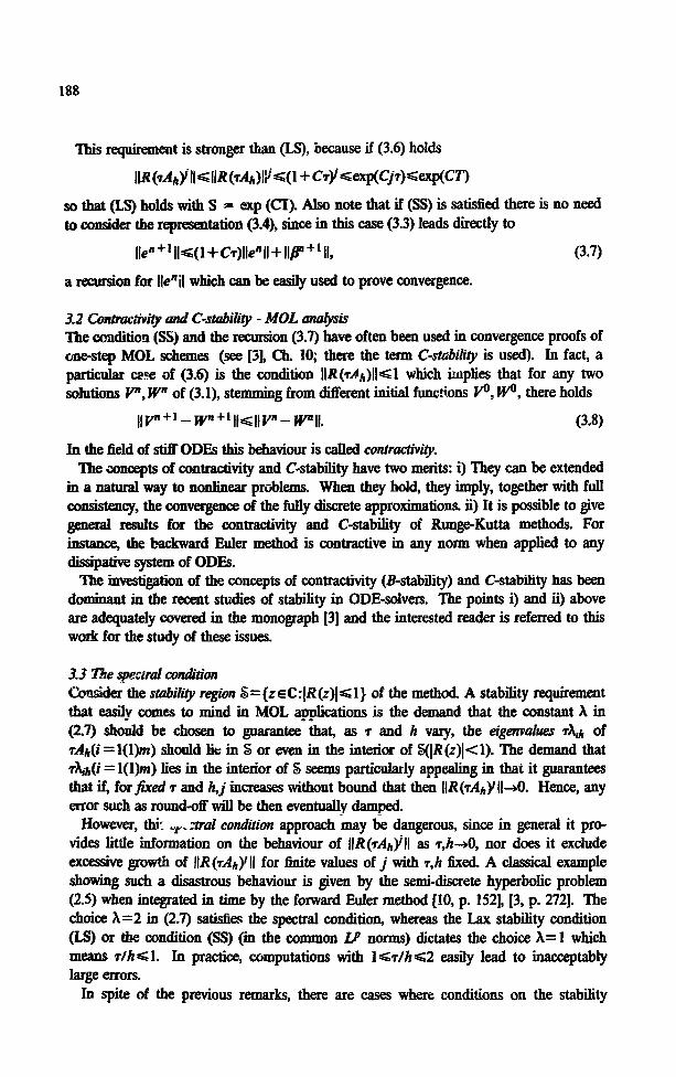
This requirement is stronger than (LS), because if (3.6) holds

IIR(~~~~IIcIIR(IAh)l~6(1+C~~6exp(C~7)6exp(CT)

so that (LS) holds with S = exp (CT). Also note that if (SS) is satisfied there is no need to consider the representation (3.4), since in this case (3.3) leads directly to

Ile”+‘ll~(1+C~)lle~II+ll~++ll, (3.7)

a recursion for Ile’Tl which can be easily used to prove convergence.

3.2 Contrac~~ity and C-stabi@ - MOL analysis The caditio~ (SS) and the recursion (3.7) have often been used in convergence proofs of one-step MOL schemes (see [3], Ch. 10; there the term C-stabiky is used). In fact, a particular cese of (3.6) is the condition llR(d~)ll4 which implies that for any two solutions P, R” of (3.1), stemming from dilferent initial functions Ve, We, there holds

lIv”+~-FP+‘llcllv”-w”II. (3.8)

In the field of stiff ODES this behaviour is called contructivi~. The amcepts of contractivity and C-stability have two merits: i) They can be extended

in a natural way to nonlinear problems. When they hold, they imply, together with full consistency, the convergence of the fully discrete approximations ii) It is possible to give general results for the contractivity and C-stability of l&urge-Kutta methods. For instance, the backward Euler method is contract&e in any norm when applied to any dissipative system of ODES.

The investigation of the concepts of contractivity (B-stability) and C-stability has been dominant in the recent studies of stabihty in ODE-solvers. The points i) and ii) above are adequately covered in the monograph [3] and the interested reader is referred to this work for the study of these issues.

3.3 T& qB?Wl co?li&tioii Courter the s&&&y region S= {z EC@ (z)I< I} of the method. A stability requirement that easily comes to mind in MOL applications is the demand that the constant X in (2.7) should be chosen to guarantee that, as T and k vary, the eigenvulues TAB of dh(i = I(l)m) should lie in S or even in the interior of S@(z)l<l). The demand that d&i = l(l)m) lies in the interior of S seems particularly appealing in that it guarantees that if, for &ed T and h,j increases without bound that then llR(d/J’Il+O. Hence, any error such as round-off will be then eventually damped.

However, thir yy_ztral condition approach may be dangerous, since in general it pro- vides little information on the behaviour of llR(d~y’II as r&+0, nor does it exclude excessive growth of llR(~&ylI for llnitc values of j with ~,h fixed. A classical example showing such a disastrous behaviour is given by the semi-discrete hyperbolic problem (2.5) when integrated in time by the forward Euler method [lo, p. 1521, [3, p. 2721. The choice X=2 in (2.7) satisfies the spectral condition, whereas the Lax stability condition (LS) or the condition (SS) (in the common Lp norms) dictates the choice h=l which means ~/hGl. In practice, computations with 1 <r//h92 easily lead to inaccqtably large errors.

In spite of the previous remarks, there are cases where conditions on the stability

region of the ODE method are suthcient to guarantee stability iu the senses (IS) or (SS): (i) If 11.11 is an inner product norm and Ah is nomud with w pect to this inner product,

then the condition TX,ES,I’=I, - - * ,m, implies lllP(~A~Y1191, j=l,Z, * - a. This

is a consequence of the fact that R(TA~~ is nomd and therefore 1IR(IAh)Ill=p(R(TAhy)=@(R(7Ar)y, where p() denotes the spectral radius.

(ii) If 11.11 is an inner product norm and the solver is A-stable then llR(~Ah)WSl, j=1,2, - * - for arbitrary T. Here is assumed that <Abvh,q,>GO for auy grid func- tion vh. This result follows from a deep theorem by VON NIWMANN [S] [7] and does not require the normali~/ of Ah.

The result by van Neumann has been recently used by SPIJKER [16] to derive an interesting su&ient condition for contractivity.

4. CONSISFBNCY ASPECTS

4.1 The stature of the @ll) local error After our review of the behaviour of the powers R(TA# we now turn our attention towards the local errors #F +‘, the other factor that p~cording to (3.4) determines the global error. Our aim is to iuvestigatc the behaviour of j.l”+’ iu terms of the smoothness in time of the PDE solution N(t) and the space truncation error a(t) introduced in

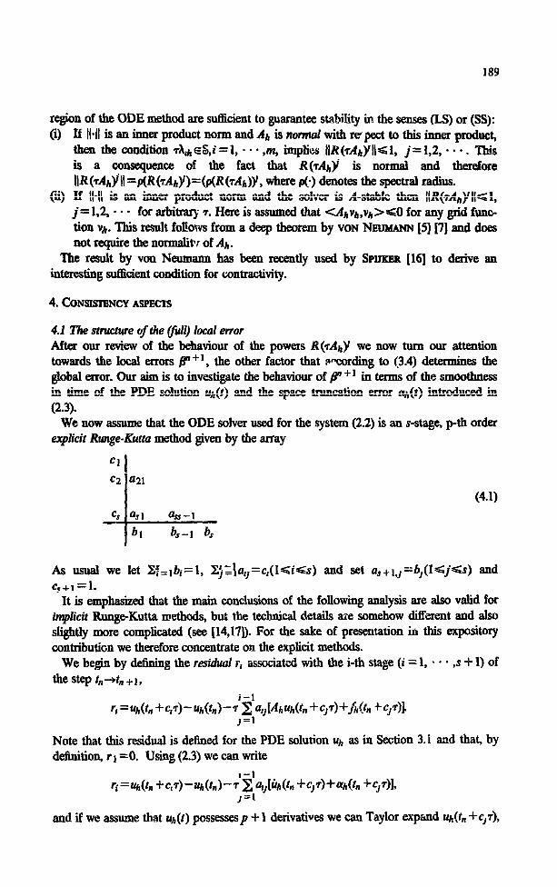
(2.3). We now assume that the ODE solver used for the system (2.2) is au r-stage, p-th order

e@ict Rtmge-Kuttu method given by the array

cs as1 ass-1

bl b-1 bs

(4.1)

As usual we let Cf=lbi=l, ZZjZ\a,,=c,(l<i~s) and set a,+l,,=b,(lGjGr) and cs+r=l.

It is emphasized that the main conchtsions of the following analysis are also valid for implicit Runge-Kutta methods, but the technical details are somehow different and also slightly more complicated (see [14,17D. For the sake of preseutation LI this expository contribution we therefore concentrate on the explicit methods.

We begin by defining the residual r, associated with the i-th stage (i = 1, - * - ,s i- 1) of the step k%+l,

Note that this residual is defined for the PDE solution uh as in Section 3.1 and that, by definition, r 1 =O. Using (2.3) we cau write

ri=a& +e,7)-nrk(t~)-7’~‘a~[Q(t. +c,r)+a/& +c,$], J=l

and if we assume that ah(t) possessesp + 1 derivatives we can Taylor expand uh(fn +cJTh

190

&(r, +cj7) $0 arrive at an expression

Here 4 are Ooeaacieuts which only depend on the array (4.1) and R, is the sum of the remainder in the Tayktr expansions plus the term du,p&m+cjT)s which is the space emx contribution.

The~~tesidualsare~forderivinganexpnessionfor~~l whichismore ameuable for the ta& we have set ourselves than the expression given in (3.2). This is done as fokws. We w&e down the ordinary RungeKutta equation (cf. (4.1))

~=v"+:~~~~-~i~+~(~~+CjT)] (19iGS+l) j=l

where tP+* =Ys+l, and thepd equations

Yk(t.+ei7)=~(t.)f:~~~[Akq(t~+q3+Ib(t~+e,rll+r, (19iCs + 1). j=I

Thenwesub~thesetwofonnulastoobtainaserofrelatioassatisfiedbythefull~~ bal errors en=u&)-U”,em+’ and the &ermdiate errors u&,+ci~)-~ (1~~s). A straightforward azxmske elimination of the latter errors leads to the mursiou (3.3) for the full global error, but with $+I now in the form

(4.3)

where & is a polyuoruiai of degree G:s + 1 -i whose dcients depend on (4.1). Note that the behaviour of these po&nomials accounts for the inter& stability of the R& schenq i.e., for the effect on u” +I 0 perturbations iu the stages of the step t,+t, + 1. f Substitition of (4.2) iu (4.3) &ally leads to thsfirll Emal error expression

F +’ =z A# ~‘A~~~(t*)+~~~a(i(rA~), (4.4) ‘Z

where Nj are Scalars which only depend 011 the parameters in (4.1) and the sumr&cm ~,jextenasta lGZ<s-I, 2GjGp,p+ld+j.

An importat pint to notice is that in (4.4) we find not only derivatives u&i)&) (that are expected to behave nicely as !mO), but also powers Af that will imrease as h+O due to the negative powers of A mntdned in Ai. Thus the malyti d c4.4) can be ~m,“,,delicate and, indeed, we will see below that the negative powers of h

.

4.2 Behaviov of the@ local error - Local order reduction The subsequent analysis is carried out under the following hypoleses: (HI) The r&r& tion ~(1) of the PDF solutiou possesses p + 1 derivatives u&t). Furthermore Iluj~(~)ll cau be bounded uniformly in z and h. (IQ) The space&me grid refkment is carried out subject to a condition (2.7) with hem and for this rekment the expression dL&II can -be bounded independently of I and h.

Hypothesis (H2) is natural here since we are discus&g explicit methods. RecaM that the order in space of (2.1) is q and that therefore the entries d A,, are expected to

191

increase like h-q. Our ta& in this subsection is to derive for II@ +I II bounds of the type

(4.5)

where C denotes a constant independent of rn,7 and h and k is a positive number. We will see that in order that the bound (4.5) be uniform in h, the exponenr k must usu@ be taken smaller thun p -I- 1, the value one naively expects from the behaviour of the RK method applied to ODEs.

Now the hypothesis (Hl) implies that in (4.4) the terms R, satisfy a bound of the form (4.5) with k=p +l. On the other hand, (HZ) implies that llQ1(d~)ll are bounded uni- formly in ~,h and therefore the second summation in (4.4) can be bounded in the form (4.5) with an optimal k =p + 1. In estimating the first sum at least two diErent settings may be considered (see 1141 for a third setting).

(Sl) If the further assumption is made that the norms Ildfrr&)(tn)ll are bounded uni- formly in t,, and h, then IIB +l II is bounded by (4.5) with k =p + 1.

(S2). If no relation is assumed between the powers of AI, and the derivatives of u&), then to bound a term like I( +JA$u$&,,) uniforn “; in h, one must write

and employ (Hl) and (H.2). The price to be paid is that for such a term the order in T is j rather than I +jZp +l. In general the local error (4.4) CoMains terms with j =2 so that in this way onZy an O(G) bound is obtained regardless qP the value of the ckusical or&p. We emphasize that this or&r reduction is not induced bi lack of smoothness in u (=s, t), but rather by the pre=ce of powers of Ah in the local error (4.4).

4.3 Behnviour of the (Fu) gIobal error - Global order reduction Once /F +I has been bounded in the form (4.5) (possibly with a reduced k, i.e.,kcp + 1) a stability assumption Iike (LS) or (SS) mentioned in Section 3.1 immediately leads to the global error bolund

(4.6)

by app@ng the standard arguments given there (cf. (3.5) or (3 7)). An important point we wish to make now is that ip k<p +l, these standard arguments of transferring the local errors to the g!_obal error (dust bounding and then adding via stability) can be landulypessimistic [1,2,14,18].

Consider (3.4) and (4.4). As already concluded in Section 4.2 the second summation in (4.4) can be bounded in the form (4.5) with an optimal k =p + 1, implying that this part of the local error causes no order problem and can be dealt with in the standard way. So we now co&e ourselves to the first sum in (4.4) and treat only one of the terms NJ+f+JA&uQ) that may suffer from reduction. The other terms can be dealt with in tbe same fashion.

According to (3.4) the term considered contributes to the global error e$ by an amount

ag=&G’J i=R(rAhr-‘Aluk)(~,-l). (4.7) r=l

Assume that the matrix (I -R(TAh))-’ IAh can be defined and satisfies a bound

ll(f-R(TAb))-lTAhII~~ (4.8)

with YI independent of T$. (The feasibility of this condition is discussed in 1141). Then (4.7) can be rewritten as

=,p _‘[(I -R(TAh))-‘TAh~[A~-‘~‘(?, _])-R(TAh~A~-‘u~‘(lo)+

“$+A# -‘Ap(ujp(rj _,)-&?,))]. i=l

Further we write

The following result now folIows easily: Suppose that as h,+r vary (4.8) holds and llR(~A~)ll< 1. Then the global error contribution a# possesses a bound of the form

QC!,a +“-‘(~l~~-‘uy+‘~li+maxlLQ~-‘u~~ll). (4.9) 9 t,h ’

The cxucid observation is that we have got rid of one power of Ah, i.e., we are now deal- ingwithA&-linsteadoftheA~ westartedwith. Thisisofimportancesincethereduc- tion emanates from the negative powers of h contained in Ah.

If we collect alI bounds (4.9) for 1,~ from their range of summation

(161Cs - 1,2Gj<p,f +J -I>p),

take into account the second summation in (4.4) and the hypotheses (IN), (H2) of se0 tion 4.2, we finally arrive at a global error bound (cf. (4.6))

Ile”ll~C(~+g~~l~(l)ll), k -1CgGp. (4.10)

The particular value of g depends on theprobkm, i.e., on the order in space q and on the possiile growth with k of the grid functions occurring in (4.9). In the worst case, where no relation is assumed between the powers of Ah and the derivatives of rq, (setting (S2)) the order in T of the individual bounds (4.9) can be put equal to j, so that if p > 1 we have g>2 in (4.10). Hence in the worst case setting it is possible that the drop in glo- bal order is one unit Iess than that in local order (see Section (4.2)). Obviously, in the set- ting (S 1) we have g =p and the speciaI derivation of this subsection is not necessaq.

In the next subsection we shall discuss a particuku example with the aim of ihustrating the analysis, but also to show that the (minimal) order g =2 in (4.10) really may occur.

4.4 An example We consider the hyperbolic model problem (2.4) with its semidiscretization (2.5). It is supposed that the solution u of (2.4) is as smooth as the analysis requires. (This assump tion implies not only that ua,fn aud fr are smooth, but also that they satisfy certain compatibility conditions whose expressions are of no consequence here). We shall work

E usual L2-norm and Lao-norm. Let I,OSxGl, be some smooth function. When the matrix Ah given by (2.5) acts

193

on the f~~c~on vh the 2”:’ - - ’ ,& entries in Ahvh approximate values of v, and can therefore be bound&I indep&denUy of h. However, the first entry in J$,vh will behave like h-* as h+O unless v satisfies the homogeneous boundary condition v(O)=O. L&e wise, the Yd, m - - $rnfh entries in &h approximate values of v, and are thus bounded. However, the fbst and second entries in &h wi! anly be bounded if v(O)= vJO)=O. The general trend should now be ckar. For I - 1 = 1,2, - - . ,s -2 (= the highest power of Ah which occurs in the bounds (4.9)), ILdi- ‘vh 11 is bounded in h if

25$LO,k=OJ,. . . ,I -2.

h &nerd, llA~-‘vhil2 behaves like h(3’2-‘j(Z>2) while in Loo we have the behaviour h(t-c).

Next, since the highest power of Ah in the bounds (4 9) is (s -2), it follows that the optimal exponent g =p in (4.10) will be obtained if the theoretical solution U&Z) satisfies s -2 boundary requirements

u(O,t)=O, u,(O,t)=O, ’ - ’ ,(r3/ax”-3)u(0,t)=0

that render it possible for Ak-‘~f/),A~-~u~+‘) (lGf<s - 1,2=Gj<~~, 4+j+ +l) to remain bounded uniformly in h. These s -2 boundary requirements for u wiU be satisfied if and only if fn ,fr do not violate a set of s - 2 constraints

jr=, fa(o,l)=o, . . . , (as -4/axs-4)fa(o,t)=o.

We emphasize that such constraints are induced by the numerical method and are not related to the compatibility conditions that jr ,fa,ua must satisfy in order that u be smooth. Perhaps it is useful to point out that for homogeneous problems (homogeneous boundary conditions and no forcing term), the above constraints are trivially satisfied and no order reduction occurs. If one or more of the constraints are not satisfied the exponent g in (4.10) can be found by a simple inspection of the differentials featuring in (4.9) crY,#O). The one with the largest reduction will determine g.

Finally, we have tacitly asumed that the number of stages s is greater than or equal to three_ No reduction will take place with a astage method, and, of course, with the Euler method.

Far the time integration of the semidiscretization (2.5) we consider the classical 4- stage, 4th order scheme

0 0 l/2 l/2 0 l/2 0 112 0 1 0 0 1 0

1 l/6 l/3 l/3 l/6

From its local error expression [14]

p+’ =(~h~~4)+~~UP’+~l~~~~ +

(&&I?) + &42UFP + &244)77 + 5 ~dTA/$$, 1=2

we deduce that mme of the coe!!ckats ~,(lCZ63,2<jC4, I+@) is zero so that all

gzid functions which feature ia (4.9) may cmtibute to a reduction of the order. Obvi- ously, the largest reduction will emanate from the two terms in (4.9) with (l +j) minimal and (Z-l) m&mal, which are here ~~Afz#) and ~~Afz#). Hence if the additional boundary quirements mentioned above (v(O)=v,(O)=O, v=&), v=uh3J) are not &is&xi and r/h is kept fixed (cf. (2.7)), we will have to face a reduction in global order from4to2ifwemeasure inLao andfrom4t02.5ifwemeasureinL2.

4.5 A nvmeri& iilt&mtion We have applied the above RK method to the semidiscretization (2.5) with the choice u(x, 0)= i+x, fr(r)= I/(l+r), f~(qt)=(t --x)/(1 +tF which yields the simple solution +-&=(I +x)/(1 +t). since this solution is linear in space, there is no error introduced by the space discre&tion (a@). The time derivatives of u are nat zero at the boun- dary so that the reducti~ mentioned in the preceding example should occur.

The floating point numb in the table below are the LSD - errors at t = 1 for certain values of qh. ‘B’he fmed point numbers represent the observed orders of convergence upon either s&u&m ludving of r,h (de numb in italics) or halving T on a&& grid Rec.& that these computed orders are given by the expression logz (error ratio).

h-’ 11 10 20 40 80

10 .ii9uJ-4 4.7 2.1

20 2610-5 .l610-4 4.2 2.0 4.7 2.1

40 .15]0-6 .6510-6 .4010-S 4.1 2.2 4.3 2.0 4.6 2.0

80 .8510-S .3&o-7 .1610-s .9710-S

For the simultaneous refincmeut the auticipatcd reduction from 4 to 2 is clearly seen. On a tied spatial grid there is no order reddon visible. Of course, tbis is the behaviour one should expect as one is now solving afied system of ODES. With our fourth order method, the order asymptoticalIy behave like C# on each fixed grid. The issue at hand is that C depends on the choice of mesh and ir~cr~.~s with decrea&g h. This is very clearly borne out in the last row of the table.

An illustration of order reduction 0xurring in a RK-finite element scheme applied to problem (2.4) can be found in 1141. The interested reader should also consult 1171 where examples with implicit RK methods applied to parabolic problems are d&cud.

4.6 Some conch&g remarks on order reduction The attention here has been restricted to linear problems. Order reduction also takes place for nonlinear problems and the mechanism involved there is essentially the one we have discus& The extension of the analysis to the nonlinear case IS possible but be-xmes rather technical and offers no new tiqight.

As ~E&IMXI earlier, for implicit RK schemes the main ideas of our analysis are still valid. However, the interest there is in situations where T and h are not related and therefore our hypotheses (HZ) should be forsaken. The details of the analysis become

195

then quite differmt [1,17]. A simple means for avoiding order reduction has been suggested and tested in [14]. It

is based on reformulating the PDE problem, prior to the space discretization, so that the additionally required boundary conditions are satisfied.

Finally, it is fair to say that in practical problems the negative effects caused by order reduction are likely to be less Qwtant than those stemming from other so- such as errors in space, instabilities at boundaries, curved boundaries, etc. However, the understanding of this phenomenon is essential in situations where one is interested in higher order methods.

[l] P. BRBNNER, M. CROUZEIX & V. THOI&E, Single step methods fir inhomogeneou linear difirential equations in Banach space, RA.I.RO. Analyse numerique 16, 5- 26, 1982.

[2] IL B-GE, W.H. HUNDSDO= BE. LG. VWWER, A srudy of B-conve~~e of Runge-Kutta metho&, Computing to appear.

[3] IL DEKKRR, & LG. VERWER, Stability of Runge-Kutta t&hot& for stiff nonlinear d@emiab equations, North-Holland, Amsterdam-New York-Oxford 1984.

[4] R F-q J. SCHNEID & C.W. UEBERENBER, or&r results for implicit Runge-Kutta methalr applied to stiflsystems, SIAM J. Numer.Anal. 22,515-534,1983.

[5] E. HMUR, G. &UWR & CH. LUBICII, On the stabilip of semi-implcit metho& for ordinary d@rential equabons, BIT 22,211-232, 1982.

[6] H.O. KREISS, Ueber die Stabilit&s&$nition @r Diflerenzengleichwtgen die partielle Differentia&eichungen approximicren, BIT 2, 153-181, 1962.

[7] P. VON NEUMANN, Eine Spek M?!zzz~+ ,%.r allg.eine Operatoren eines uniriiren Raumes, Mathematish~ Nachrichten 4,258-281, 1951.

[8] C. PNENCIA & J.M. %NZ-&RNA, Equivalence theorems for incomplete spaes: an qpraisal IMA. J. Numzr. Anal. 4, 109-115, 1984.

[Yj C. PALJZNCIA & J.M. SANZ-SERNA, An extension of the Last-Richtmeyer tkory, NUUXX. M&h. 44,279-283, 1984.

[lo] RD. Bxwrr.w~~ & K.W. MORTON, Di$eence methods for mitial vak problems, &.&Tsc&~~ Publishers, ?+Iew York-London-Sydney, 1967.

[l l] J.M. SAN&T&w& Convergent approximation to partial differential eqttations and sta- bility concepts of metho& for stiflsystenu of ordinary aQ$erential equations, Actas del VI CEDYA, Jaca, University of Zaragoza, 1984 (availzble on request from J-MS.).

[12] J.M. SANZ-Z&RNA, Stabiliy and convergence in Munerical Analysis I: Linear prob- &PLT, a simple, comprehensive account, ti NOF%MW Ukentia3i qsztio~ and appli- c&ions, J. Hale and P. Martinez-Amores (eds.), Pitman, Boston, pp. 64-l 13, 1985.

f13] J.M. SANZ-&RNA & C. PALENCIA, A general equvalence theorem in the thewy of discretizatron methods, Math. Comp. 45, 143-152% 1985.

[14] J.M. SANZ-SERNA, J.G. VERWER & W.H. HUNDSDORFER, Cclprvergence and order

reduction of Runge-Kutta schemes applied to evoiztionary problems m partial direntral equations, Report NM-R8525, Centre for Math. and Comp. SC., hter-

dam, 1985. 1151 J.M. SANZ-!&RNA & MN. SPIJKER, Regrons of stability, equivalence theorems and the

Courant-Iariedrich&ewy condition, to appear in Numer. Math.

196

[ 16J MN. SPUKER, Stepssize restrictions for stabi&y of one-stq method IP the mntenutl sabiion of in&l vaheprob?km~, Math. c.‘omp. 45,377-392,198s.

[17j LG. VERWER, Ctmwgence and or&r reduction of dingonalij implicit Rung& Kutta schemes in he met!xdof lines, Report NU-R8506, Centre for Math. and Camp. SC., Amsterdam, 1985 (to appear in Proc. Dundee Num. Anal. Conf. 1985).

118) J.G. VERWER & J.M. SANZ-SERNA, Comwgence of method of lhes qproximatims to partial dirmtial equatiom Computing 33,297-313,1984.