conversion between sine wave and square wave spatial ...conversion between sine wave and square wave...

M T R 0 1 B 0 0 0 0 0 2 1

M I T R E T E C H N I C A L R E P O R T

Conversion Between Sine Wave andSquare Wave Spatial FrequencyResponse of an Imaging System

July 2001

Norman B. Nill

Sponsor: DOJ/FBI Contract No.: DAAB07-01-C-C201Dept. No.: G034 Project No.: 0701E02X

Approve for public release; distribution unlimited.

© 2001 The MITRE Corporation

Center for Integrated Intelligence SystemsBedford, Massachusetts

iiiiii

Abstract

The spatial frequency response of an imaging system, known as the Modulation TransferFunction (MTF), is a primary image quality metric that is commonly measured with asine wave target. The FBI certification program for commercial fingerprint capturedevices, which MITRE actively supports, has an MTF requirement. In some cases,however, a square wave ("bar target") must be used in testing, which results in a similarquantity called the Contrast Transfer Function (CTF). This document reports on aninvestigation of the mathematical relationship between the MTF and CTF, methods forconverting between the two, and derives an equivalent CTF from the given spec MTF, foruse in the FBI certification program. The methodology presented is applicable to thegeneral case, i.e., whenever conversion between the MTF and CTF of an imaging systemis needed.

vv

Table of Contents

Section Page

1. Introduction 1 1.1 Background 1 1.2 Problem Statement 5

2. Problem Solution - Synopsis of Results 7

3. Technical Details of Solution 11 3.1 Solution Approach 11

3.1.1 Methodology 11 3.1.2 Computer Program 15 3.1.3 Results 16

3.2 Alternative Approach - Coltman Formula 19 3.3 CTF Normalization 23

List of References 25

Appendix Computed CTFs 27

Glossary 35

viivii

List of Figures

Figure Page

1. Typical Sine Wave Target 4

2. Path of Single Sine Wave to Generate MTF Data Point 2

3. Curve Fits to Spec MTF / Sinc(πfw) 14

4. Computed 500 ppi CTFs for 5, 15, 50-Bar Targets and Spec MTF 17

5. Computed 1000 ppi CTFs for 5, 15, 50-Bar Targets and Spec MTF 17

6. Final Spec CTFs Compared to Original Spec MTFs 18

7. Variations of Coltman Formula Application 21

8. Lens CTF Calculated via Coltman and Section 3.1 Method 22

List of Tables

Table Page

1. IQS Spec MTFs and Corresponding, Proposed Spec CTFs 9

viiiviii

1

Section 1

Introduction

1.1 Background

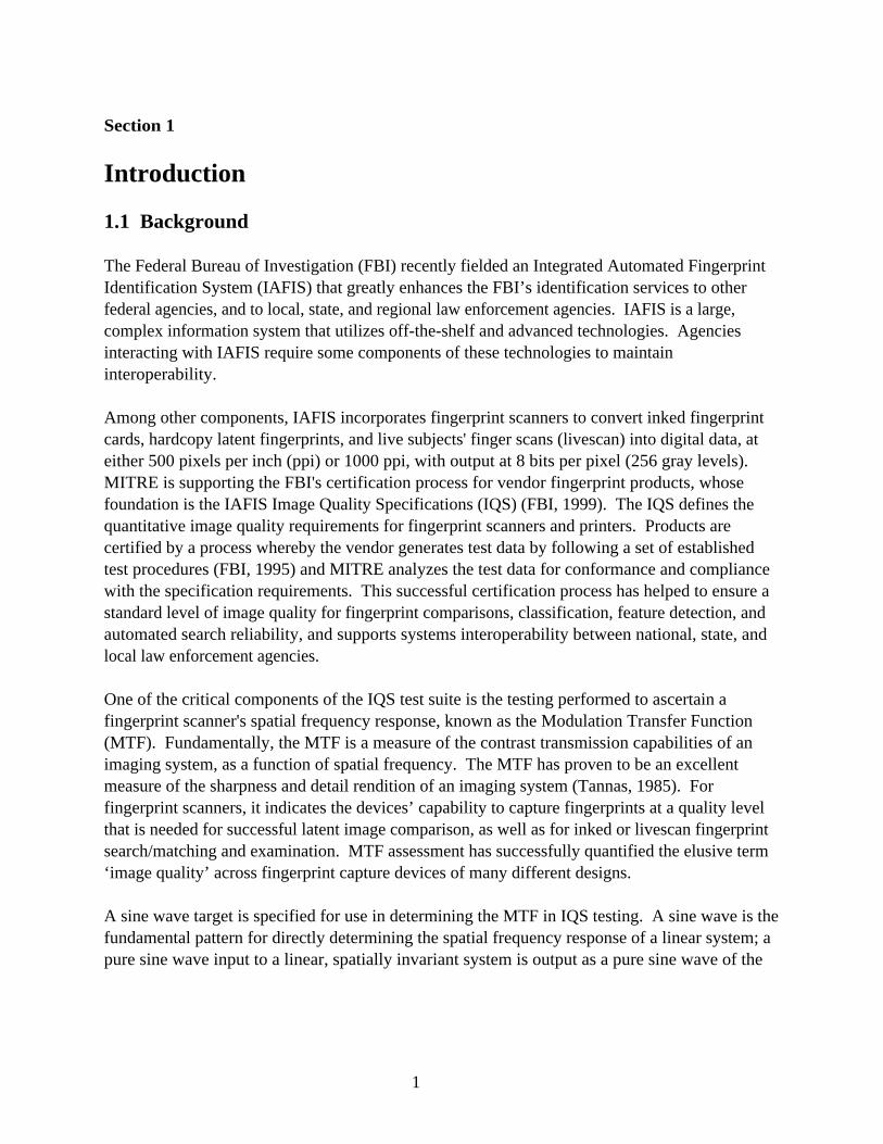
The Federal Bureau of Investigation (FBI) recently fielded an Integrated Automated FingerprintIdentification System (IAFIS) that greatly enhances the FBI’s identification services to otherfederal agencies, and to local, state, and regional law enforcement agencies. IAFIS is a large,complex information system that utilizes off-the-shelf and advanced technologies. Agenciesinteracting with IAFIS require some components of these technologies to maintaininteroperability.

Among other components, IAFIS incorporates fingerprint scanners to convert inked fingerprintcards, hardcopy latent fingerprints, and live subjects' finger scans (livescan) into digital data, ateither 500 pixels per inch (ppi) or 1000 ppi, with output at 8 bits per pixel (256 gray levels).MITRE is supporting the FBI's certification process for vendor fingerprint products, whosefoundation is the IAFIS Image Quality Specifications (IQS) (FBI, 1999). The IQS defines thequantitative image quality requirements for fingerprint scanners and printers. Products arecertified by a process whereby the vendor generates test data by following a set of establishedtest procedures (FBI, 1995) and MITRE analyzes the test data for conformance and compliancewith the specification requirements. This successful certification process has helped to ensure astandard level of image quality for fingerprint comparisons, classification, feature detection, andautomated search reliability, and supports systems interoperability between national, state, andlocal law enforcement agencies.

One of the critical components of the IQS test suite is the testing performed to ascertain afingerprint scanner's spatial frequency response, known as the Modulation Transfer Function(MTF). Fundamentally, the MTF is a measure of the contrast transmission capabilities of animaging system, as a function of spatial frequency. The MTF has proven to be an excellentmeasure of the sharpness and detail rendition of an imaging system (Tannas, 1985). Forfingerprint scanners, it indicates the devices’ capability to capture fingerprints at a quality levelthat is needed for successful latent image comparison, as well as for inked or livescan fingerprintsearch/matching and examination. MTF assessment has successfully quantified the elusive term‘image quality’ across fingerprint capture devices of many different designs.

A sine wave target is specified for use in determining the MTF in IQS testing. A sine wave is thefundamental pattern for directly determining the spatial frequency response of a linear system; apure sine wave input to a linear, spatially invariant system is output as a pure sine wave of the

2

same frequency, generally with reduced amplitude1. It has a high signal-to-noise ratio, and thefact that each spatial frequency is individually imaged has been found to be very useful in faultdetection/isolation of scanner problems. In addition, the maximum value MTF is the IQS-specified quantity of interest and a sine wave target readily lends itself to such a measurement,because the single sine period in each frequency pattern that exhibits the highest computedmodulation can be readily identified. Finally, the target is available as a commercial off-the-shelfproduct2; a typical sine wave target is shown in Figure 1.

Figure 1. Typical Sine Wave Target

1 Other targets can be used to measure the MTF, e.g., a narrow line target, point target, random pattern, or sharpedge. In these cases the target is broken up into its sine wave components, via Fourier analysis, to compute the sinewave MTF. Each target type has its own set of advantages and disadvantages.

2 Three vendors (first is manufacturer): http://www.sinepatterns.com, http://www.edmundoptics.com,http://www.jmloptical.com

gray patchesfor I/O response

sine wavepatterns

http://www.sinepatterns.com

http://www.edmundoptics.com

http://www.jmloptical.com

3

For IQS testing, the sine wave target is scanned and the resulting digital image is processedthrough a MITRE-developed computer algorithm which computes the scanner’s MTF (MITRE,2001). The essence of the technique is illustrated in Figure 2 for a single sine wave frequency: thegray levels corresponding to the peak and valley in the sine wave image are identified, these graylevels are converted to target space reflectance values by traversing the scanner's input/outputresponse curve, the image modulation is computed, and divided by the target modulation toobtain a single point on the MTF curve. The process is then repeated for a series of sine wavefrequencies until the complete MTF curve is generated.

A complication in applying the MTF concept to image scanners results from the fact thatscanners perform discrete sampling over finite areas. A scanner samples a continuous, analogimage input at discrete locations over discrete time intervals, integrating all incident light energyover a given time interval and within a small area around each sampling point, where the smallarea is the individual detector element ("pixel") area. One of the consequences of this discretesampling by finite-sized detector elements is that the scanner acts as a space variant system,which implies that the scanner MTF can be multivalued (Park, et.al, 1984; Feltz, et.al., 1990). Inthe context of the sine wave target, this space variance means that the phase between this targetand the scanner's detector array plays a role in the actual MTF achieved. Here, phase refers tothe location of the detector pixel within a sine wave period, at the time the pixel is collecting lightenergy. As the target-detector phase changes, the scanner MTF can change, within limits. Inpractice, one measures the minimum, maximum, or average MTF. It has been establishedprocedure in IQS testing to use the maximum measured MTF (after noise filtering) for comparingto the spec MTF for compliance verification purposes.

4

Figure 2. Path of Single Sine Wave to Generate MTF Data Point

max

minDistance

Brig

htne

ss

Linear System

Sine Target

Sine Image

image modulation =

image mod

target modMTF =

Spatial Frequency

1.0

Mo

du

lati

on

MTFG

ray

leve

l

tgt R

img gray

Rmax - Rmin

Rmax + Rmin

5

1.2 Problem Statement

There are two fundamentally different types of fingerprint scanners certified for use in the FBIIAFIS program. In one type, inked fingerprints on card stock ("ten-print card") or latent printson paper are scanned. Typically, this scanner is a general purpose, Commercial-Off-The-Shelf(COTS) or modified COTS flatbed, desktop scanner operating in reflection mode, with a linearCharge-Coupled Device (CCD) scanning array detector and associated signal processing toproduce the digital output image. The common imaging mode utilized in these scanners is alwayscompatible with scanning a reflective sine wave target.

The other type of scanner, here called a livescanner, directly scans a person's finger and isdesigned solely for that purpose. In the most common livescanner design a subject's finger ispressed against ("plain impression") or rolled across ("rolled print") the surface of a glass prism.The image is created by the difference in index of refraction (n) between skin and air, utilizing theoptical imaging principle of "total internal reflection" (TIR), also called "frustrated internalreflection" (FIR) (Smith, 1966). Within certain defined angles of incident illumination, lighttraveling from the prism surface to finger ridges in contact with the glass will be absorbed by theskin (nglass ≅ nskin), while light traveling from the prism surface to finger valleys, where a glass-airgap exists (nglass > nair), will be reflected back into the glass. The reflected light is detected by alinear or two-dimensional CCD array to produce the digital output image.

FIR imaging in livescanners depends on the three-dimensionality of skin, which is either incontact or not in contact with a glass surface, and the relative indices of refraction between glass,air, and skin. Many livescanners cannot adequately image a two-dimensional, continuous graytone sine wave target; the output image suffers from low signal-to-noise ratio, low contrast, andvery few gray levels, making it impractical to compute a valid MTF. It has been found throughexperimentation, however, that livescanners can adequately image reflective or transmissive bartargets, mainly because a bar target is extremely high contrast with only two gray levels, blackand white, and it can be easily fabricated on a glass substrate.

The fundamental problem addressed in this document can be stated as follows:The FBI image quality specification specifies the minimally acceptable values for a scanner MTFwhen it is measured using a sine wave target. Since a bar target must be used in some productcertification cases, the problem is to answer the questions: (1) is there a relationship between thespatial frequency response derived from a bar target and the MTF derived from a sine wavetarget?, (2) what is this relationship?, and (3) what is the best approach for handling a bar targetderived spatial frequency response, given that the specification is for a sine wave target derivedMTF?

7

Section 2

Problem Solution - Synopsis of Results

The analyses and theory presented over the years in technical literature confirms that, for thesame imaging system, the bar target derived spatial frequency response and sine target derivedMTF are not equal to each other, but, as will be seen, there is a definite mathematical relationshipbetween them. The difference between the two quantities is often highlighted by denoting thespatial frequency response obtained from a bar target as the Contrast Transfer Function (CTF) orsquare wave response, to distinguish it from the term 'MTF', which is reserved for the sine wavetransfer function. This terminology distinction between bar target CTF and sine target MTF isused in the remainder of this document.

In solving the problem at hand, where a sine wave target MTF is specified but the imagingsystem under test may require use of a bar target, one can either:

(1) convert the spec sine wave MTF to the equivalent bar CTF, which then becomes the spec CTF when bar targets are used,or,(2) convert each CTF measured with a bar target to its equivalent sine wave MTF, for comparison to the original spec sine wave MTF.

The first approach is more straightforward to apply in the testing environment, with less chanceof computational error, because the modulations of a sample are directly computed from the bartarget image and compared to the 'spec' bar CTF, with no further manipulation or conversion ofsample data. Therefore, the first approach is the solution approach utilized.

The method of construction of the spec CTFs are discussed in detail in Section 3; here wepresent the final results in terms of the proposed spec CTFs for IQS certification complianceverification. Table 1 gives the proposed spec CTFs for a 500 ppi scanner and for a 1000 ppiscanner, which are equivalent to the corresponding IQS Appendix F spec sine wave MTFs, alsogiven in Table 1 (see also Figure 6). The following points should be noted with respect toTable 1:

• The CTF values in Table 1 are unnormalized and assume a target modulation of 1.0 at allfrequencies.

8

• In IQS testing, the bar target frequencies cannot be predefined because the exact target, eitherCOTS or special design, is a vendor choice. The actual CTF is moderately dependent on thenumber of bars at a given frequency; Table 1 values are the average of 5-bar, 15-bar, and 50-barCTFs. A bar target with less than 5 bars per frequency should never be used for CTFmeasurement3.

• For a bar target containing frequencies not given in Table 1, the following equations can be usedto obtain the CTF modulation values at those other frequencies.

500 ppi, f = 1.0 to 10.0 cy/mm,CTF = 3.04105E - 04* f 2 − 7.99095E - 02 * f +1.02774 (1)

1000 ppi, f = 1.0 to 20.0 cy/mm,CTF = −1.85487E - 05* f3 +1.41666E - 03 * f2 − 5.73701E - 02 * f + 1.01341 (2)

3 A 3-bar target, such as the USAF 1951 tribar target, is not appropriate for CTF measurement because the peak andvalley image amplitudes are erratic, only the center bar and two adjacent spaces are available for modulationcalculation, and because obtaining good phasing between the target and scanner detector pixels is difficult. Aminimum of a 5-bar target is required for stability, such as the NBS 1010A target (a.k.a., NBS 1963A target,ANSI/ISO Test Chart #2); better is a 15-bar target, such as the T90 target.

9

Table 1. IQS Spec MTFs and Corresponding, Proposed Spec CTFs

Frequency(cy/mm)

MTF500 ppi

CTF500 ppi

MTF1000 ppi

CTF1000 ppi

0.5 0.978 0.9791.0 0.905 0.948 0.925 0.9571.5 0.909 0.9302.0 0.797 0.869 0.856 0.9042.5 0.830 0.8793.0 0.694 0.791 0.791 0.8543.5 0.752 0.8294.0 0.598 0.713 0.732 0.8054.5 0.674 0.7825.0 0.513 0.636 0.677 0.7605.5 0.597 0.7386.0 0.437 0.559 0.626 0.7166.5 0.521 0.6957.0 0.483 0.6757.5 0.446 0.6558.0 0.312 0.408 0.536 0.6368.5 0.370 0.6179.0 0.333 0.5989.5 0.296 0.580

10.0 0.200 0.259 0.458 0.56310.5 0.54611.0 0.52911.5 0.51312.0 0.392 0.49712.5 0.48113.0 0.46613.5 0.45114.0 0.336 0.43714.5 0.42315.0 0.40915.5 0.39516.0 0.287 0.38216.5 0.369170 0.35617.5 0.34418.0 0.246 0.33218.5 0.31919.0 0.30819.5 0.29620.0 0.210 0.284

11

Section 3

Technical Details of Solution

A straightforward series expansion formula derived nearly half a century ago (Coltman, 1954)will quite accurately convert a linear imaging system's sine wave target MTF to its equivalent bartarget CTF, or vice versa, under certain conditions. These conditions include the assumption thatthe imaging system is analog, e.g., a photographic film camera, and the assumption that thenumber of target bars is infinite, i.e., the bar target is a true square wave of infinite extent. TheColtman formula and its application is described in more detail in Section 3.2, but note that theimplicit assumptions in this formula do not hold for the case of interest here. Specifically, adigital scanner is a discrete sampling system, not a continuous analog system, and a real bar targetused to measure the CTF contains a finite number of bars, sometimes as few as 5 bars perfrequency. Under these conditions, and using a curve extrapolation strategy, the Coltmanformula can still give a reasonably accurate CTF, as discussed in Section 3.2.

However, we seek a method for converting the MTF to the CTF which directly takes intoaccount the discrete sampling of a digital scanner, the finite number of bars in a bar target, andresults in a high accuracy CTF, which is a true-equivalent of the FBI's IQS specified sine waveMTF. The method developed in Section 3.1 meets these conditions.

3.1 Solution Approach

3.1.1 Methodology

The following procedure was developed for converting a discrete sampling imaging system'sMTF to its equivalent CTF for a given number of target bars:

(a) the given system MTF is divided by the Fourier transform of the sampling pixel,(b) the result of (a) is multiplied by the Fourier transform of the bar target,(c) the result of (b) is Fourier transformed,(d) the result of (c) is convolved with the sampling pixel, and(e) the maximum and minimum values from the result of (d) are located, from which the CTFmodulation values are computed.

Steps a-e are illustrated in the following math-graphic, where F denotes Fourier transformationand ⊗ denotes convolution. Steps a-e are individually discussed in detail in the following.

12

Step (a) - For an analog imaging system, the MTF can be measured up to the frequency at whichthe MTF goes to zero, which is commonly called the 'cut-off' spatial frequency in the opticalfield, equivalent to the 'band-limit' frequency in electrical engineering parlance. This step isperformed in order to obtain the imaging system MTF out to its cut-off frequency, i.e., in analogspace, before the image is sampled by the discrete detector pixels. For the case at hand, the givensystem MTF is the FBI IQS spec MTF, which is truncated at the sampling pixel's Nyquistfrequency, where the modulation is non-zero4. In equational form, the procedure is given by:

M(f) =Ms (f)

sinc(πfw)(3)

where,M(f) = imaging system MTF before discrete detector samplingMs(f)= total imaging system MTF = IQS spec MTFsinc(πfw) = sin(πfw) / πfwf = spatial frequency in cy/mmw = detector pixel width: 0.0508 mm for 500 ppi, 0.0254 mm for 1000 ppi

Since the spec MTF is only defined up to Nyquist frequency, extrapolation must be used toextend M(f) until it reaches zero modulation. A reasonable approach is to monotonically andsmoothly decrease modulation beyond Nyquist until it reaches zero. This was obtained by fixingthe zero modulation at four times the Nyquist frequency and fitting a smooth curve betweenNyquist and four times Nyquist frequency. This approach makes sense because M(f) isessentially the scanner's optics MTF and an optics MTF is everywhere positive and smoothly,

4 The Nyquist frequency equals the reciprocal of twice the pixel pitch, where pixel pitch is the pixel-center-to-adjacent-pixel-center distance. In a real scanner, the pixel pitch may be greater than or equal to the pixel width. Forexample, for 500 ppi sampling output with a scanner having a true optical resolution of 1000 ppi, the pixel pitch =1/500 = 0.02" while the pixel width is 0.01". For a discrete sampling system, valid MTF measurements cannot beobtained above Nyquist frequency. The spec MTF has a value of 0.2 modulation at Nyquist frequency but a scannercould have a value as high as ~0.7 at Nyquist. In either case, the MTF curve is truncated at Nyquist, making itcomputationally intractible.

F[ specMTFsinc(.) X F{ }

bar tgt ]

pixel

eval max & min

x

13

monotonically decreases to zero frequency5. Experiments run demonstrate that CTF results upto Nyquist frequency are not greatly affected by any reasonable choice of M(f) values aboveNyquist frequency.

For computational efficiency, a curve fit to the entire M(f) was performed, with the followingresults for 500 ppi and 1000 ppi MTFs; also plotted in Figure 3.

500 ppi, f ≤ 10.0 cy/mm:M(f)= 4.8597E-07 *f 7 - 1.856125E-05*f 6 + 2.846349E- 04*f 5 - 2.300554E-03*f 4

+ 1.060994E-2*f 3 - 2.276723E- 2*f 2 - 7.703449E- 2*f + 1.0000090 (4)

500 ppi, f > 10.0 cy/mm:M(f)= exp(−9.991357E− 02 *f1.06) (5)

1000 ppi, f ≤ 20.0 cy/mm:M(f) = -2.99661568E-8*f 5 + 3.04795483E-6*f 4 - 1.35961019E-4*f 3

+ 3.9614024E- 3*f 2 - 7.76516183E- 2*f + 1.00001941 (6)

1000 ppi, 20.0 < f ≤ 80.0 cy/mm:M(f) = -9.90555556E- 7*f3 + 2.1147619E- 4*f 2 - .0184142778E0*f + 0.627922857 (7)

Steps (b), (c) - These steps are conveniently performed by utilizing a closed form equation forcomputing the image profile of an N-bar target, given a system MTF, that has been reported inthe literature (Barakat and Lerman, 1967, Equation (10)). With a change of notation, Barakat'sEquation (10) becomes:

j(x) =1

3πcos(2πxf )sin(4πNLf )M( f )

f cos(2πLf )0

fc

∫ df (8)

where,j(x) = image intensity profile as a function of distance x, prior to pixel samplingN = number of bars in bar target, at specific frequencyL = half-bar widthfc = cut-off frequency of M(f): 40 cy/mm for 500 ppi, 80 cy/mm for 1000 ppi

5 For the special cases, not considered here, of optics with large aberrations, large defocus, or a central obscuration(apodized aperture), the optics MTF still goes to zero, but not necessarily monotonically. Also note that, at firstglance, it might seem that the spec MTF could be extrapolated first, and then divided by sinc(.); but this approachwould not give a smooth result because sinc(.) oscillates and goes through zero modulation, at frequencies above2xNyquist.

14

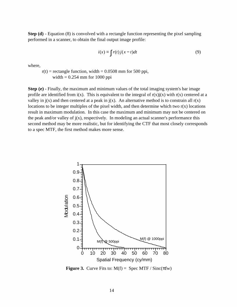
Step (d) - Equation (8) is convolved with a rectangle function representing the pixel samplingperformed in a scanner, to obtain the final output image profile:

i(x) = r(t) j(x − t)dt∫ (9)

where,r(t) = rectangle function, width = 0.0508 mm for 500 ppi, width = 0.254 mm for 1000 ppi

Step (e) - Finally, the maximum and minimum values of the total imaging system's bar imageprofile are identified from i(x). This is equivalent to the integral of r(x)j(x) with r(x) centered at avalley in j(x) and then centered at a peak in j(x). An alternative method is to constrain all r(x)locations to be integer multiples of the pixel width, and then determine which two r(x) locationsresult in maximum modulation. In this case the maximum and minimum may not be centered onthe peak and/or valley of j(x), respectively. In modeling an actual scanner's performance thissecond method may be more realistic, but for identifying the CTF that most closely correspondsto a spec MTF, the first method makes more sense.

Figure 3. Curve Fits to: M(f) = Spec MTF / Sinc(πfw)

0

0.1

0.2

0.3

0.4

0.5

0.6

0.7

0.8

0.9

1

0 10 20 30 40 50 60 70 80Spatial Frequency (cy/mm)

M(f) @ 1000ppiM(f) @ 500ppi

15

3.1.2 Computer Program

A computer program was developed in Fortran-90 to perform steps b–e, which incorporates theseparately computed curve fits given in Equations (4-7). Some features of this computer

program are as follows:

• Calculations are performed in double precision mode.

• Integrations are performed via Simpson's rule with a large number of small integrationincrements to account for the high frequency oscillations of the trig functions.

• Evaluation is only performed over 1.25 periods of the bar target, centered on the middle bar,because the highest peak and lowest valley always occur at and adjacent to the middle bar in thissymmetrical model.

• The input bar target is assumed to have a modulation of 1.0.

A number of code verification tests were run; the major tests were as follows:

• Identified required integration increments by running series of increment sizes and observingwhere stable output occurred.

• Processed a 50-cycle sine wave target with 0.0508 mm and 0.0254 mm sampling pixel widthsand with the 500 ppi and 1000 ppi spec MTFs, respectively. The output MTF should equal theoriginal spec MTF in each case, which they did to within less than 0.4% for 500 ppi case and towithin less than 0.7% for the 1000 ppi case; these results are given in the printouts in theAppendix. The errors that did occur are due to a combination of the inevitable computationalerrors and small errors in the curve fits to the input MTFs. Note that for this case of a sine wavetarget input replacing a bar target input, Equation (2) has a different denominator, given by: f [ 1-(4Lf)2 ].

• Processed bar targets, with various numbers of bars, with a diffraction-limited optics MTF; thelatter is a known, closed form equation out to the optics cut-off frequency. The output CTFswere accurate to within the accuracy that could be extracted from published data (Bass andVanStryland, 1994).

• Verified that the polynomial curve fits to the MTFs in step (a) were smooth, monotonicallydecreasing curves with no 'hidden' dips or spikes.

16

3.1.3 Results

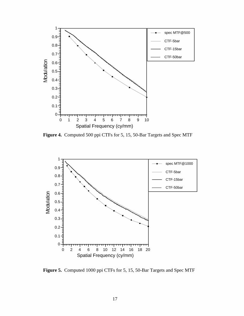
The CTF results for bar targets containing 5, 15, and 50 bars are plotted in Figures 4 and 5 for the500 ppi case and 1000 ppi case, respectively. Note that the CTF approaches a 'steady state' asthe number of target bars increases, e.g., there is very little difference between the 15 bar and 50bar CTFs. At the opposite extreme, however, for a low number of 5 target bars, there is adistinct rise in the CTF.

The most relevant spec CTF, for comparison to test data results from a real scanner, would be touse the spec CTF derived from the same number-of-bars target as is actually used in the testing.This is impractical, however, because of the wide variety of bar target designs, both COTS andspecially fabricated, which, for example, could have a different number of bars in each frequencypattern in the same target. Because nearly all practical bar targets would in fact have between 5and 50 bars at any given frequency, it is convenient to define a single spec CTF as the average ofthe 5, 15, and 50 bar CTFs. Taking this one step further, the final spec CTFs at 500 ppi and1000 ppi are defined as the curve fits to the average bar CTFs, which are shown in Figure 6 (seealso Table 1). Note that, as fully expected by the underlying theory, the spec CTFs areeverywhere higher than their respective spec MTFs.

One processing anomaly did occur. The CTF values calculated in the neighborhood of 2/3 of theNyquist frequency, i.e., close to 6.56 cy/mm for 500 ppi and 13.12 cy/mm for 1000 ppi, showedan unnatural dip in modulation; the calculated values are only about 92% of what would beexpected from a smooth curve. Some effort was expended in trying to track down the cause ofthis but it remains an unknown. The values near 2/3 Nyquist are reported in the Appendix butwere not used in generating the spec CTFs because they are believed to be anomalous datapoints, i.e., 6.5 cy/mm for 500 ppi; 12.5 and 13.0 cy/mm for 1000 ppi computed modulationvalues were not used.

17

Figure 4. Computed 500 ppi CTFs for 5, 15, 50-Bar Targets and Spec MTF

Figure 5. Computed 1000 ppi CTFs for 5, 15, 50-Bar Targets and Spec MTF

0

0.1

0.2

0.3

0.4

0.5

0.6

0.7

0.8

0.9

1

0 1 2 3 4 5 6 7 8 9 10

spec MTF@500

CTF-5bar

CTF-15bar

CTF-50bar

Spatial Frequency (cy/mm)

0

0.1

0.2

0.3

0.4

0.5

0.6

0.7

0.8

0.9

1

0 2 4 6 8 10 12 14 16 18 20

spec MTF@1000

CTF-5bar

CTF-15bar

CTF-50bar


mailto:MTF@500

mailto:MTF@1000

18

Figure 6. Final Spec CTFs Compared to Original Spec MTFs

0

0.1

0.2

0.3

0.4

0.5

0.6

0.7

0.8

0.9

1

0 2 4 6 8 10 12 14 16 18 20


CTF 1000

CTF 500

MTF 1000MTF 500

19

3.2 Alternative Approach - Coltman Formula

For analog imaging systems, such as a photographic film camera, it is possible to measure the sinewave MTF up to the frequency at which the MTF goes to zero, which is called the 'cut-off'spatial frequency in the optical field, equivalent to the 'band-limit' frequency in electricalengineering parlance. For this case, a simple series expansion formula derived nearly half acentury ago (Coltman, 1954) will quite accurately convert the square wave CTF to its equivalentsine wave MTF, or vice versa.

Given the CTF, the Coltman formula to determine the MTF, is

M(f) =π

4C(f) +

C(3f)

3−

C(5f)

5+

C(7f)

7+

C(11f)

11−

C(13f)

13−

C(15f)

15−

C(17f)

17+

C(19f)

19...

(10)

and given the MTF, the Coltman formula to determine the CTF, is

C(f) =4

πM(f) −

M(3f)

3+

M(5f)

5−

M(7f)

7+

M(9f)

9−

M(11f)

11+

M(13f)

13−

M(15f)

15+

M(17f)

17−

M(19f)

19...

(11)

where, M(f) = sine wave MTFC(f) = bar target CTFf = spatial frequency

Note that Equation (10) is an irregular sequence in terms of sign and term constants, whereasEquation (11) is a strictly alternating, sequential series. The practical application of the formulacan be illustrated by the following simple example. Suppose a CTF has been measured with a bartarget out to an imaging system's cut-off frequency of 30 cy/mm, then to compute the sine waveMTF at a single frequency, f = 2 cy/mm, requires use of the CTF modulation values at f = 2, 6,10, 14, 22, 26, and 30 cy/mm, i.e.,

M(2) =π4

C(2) +C(3 ∗2)

3−

C(5∗ 2)

5+

C(7 ∗ 2)

7+

C(11∗ 2)

11−

C(13∗ 2)

13−

C(15∗ 2)

15

(12)

The fact that the frequency of evaluation increases with each succeeding term in the expansionsgiven in Equations 10 and 11 indicates that for evaluation at higher and higher frequencies, fewerand fewer terms are used, because no modulation values are available above the cut-off frequency.In fact, for evaluation frequencies greater than 1/3 of the cut-off frequency, only the first termexists, resulting in the simple relationships,

M(f) =π4

C(f) and C(f) =4

πM(f) , for f >

cut - off frequency

3

20

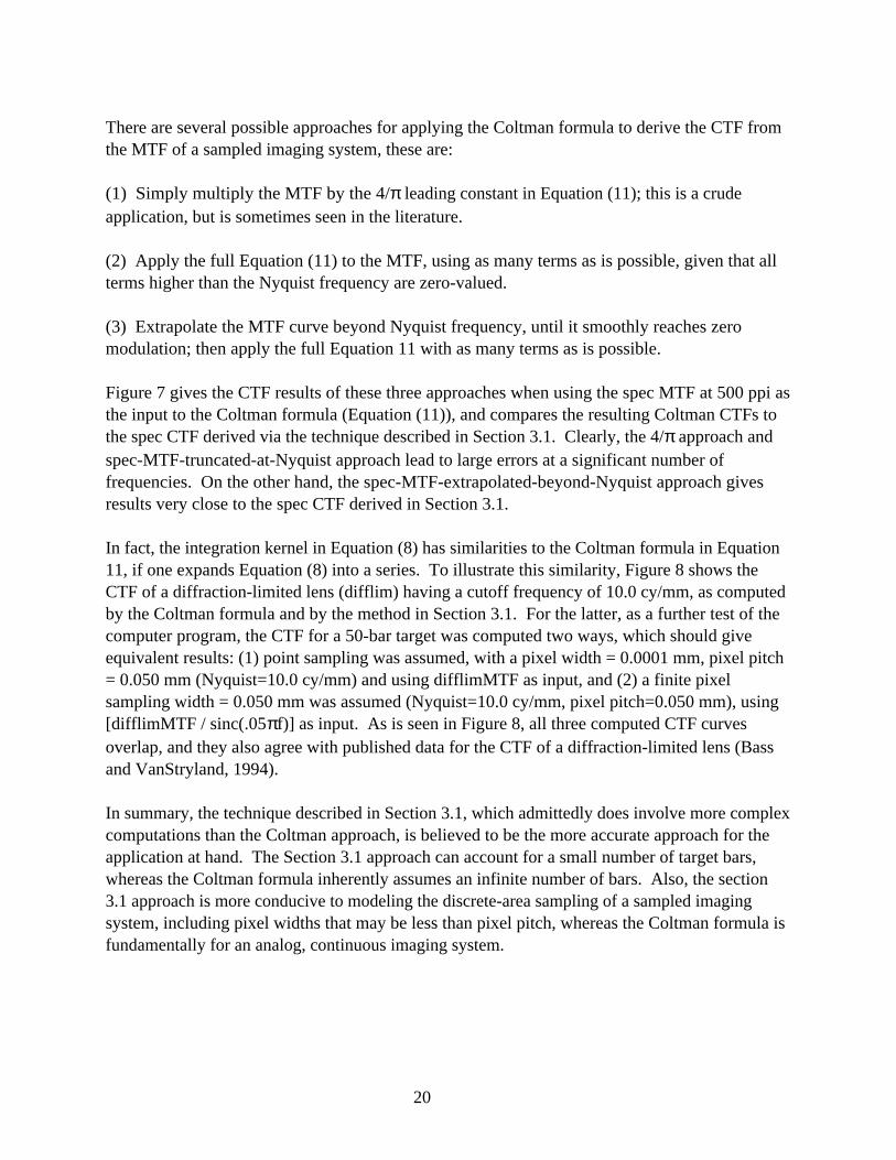
There are several possible approaches for applying the Coltman formula to derive the CTF fromthe MTF of a sampled imaging system, these are:

(1) Simply multiply the MTF by the 4/π leading constant in Equation (11); this is a crudeapplication, but is sometimes seen in the literature.

(2) Apply the full Equation (11) to the MTF, using as many terms as is possible, given that allterms higher than the Nyquist frequency are zero-valued.

(3) Extrapolate the MTF curve beyond Nyquist frequency, until it smoothly reaches zeromodulation; then apply the full Equation 11 with as many terms as is possible.

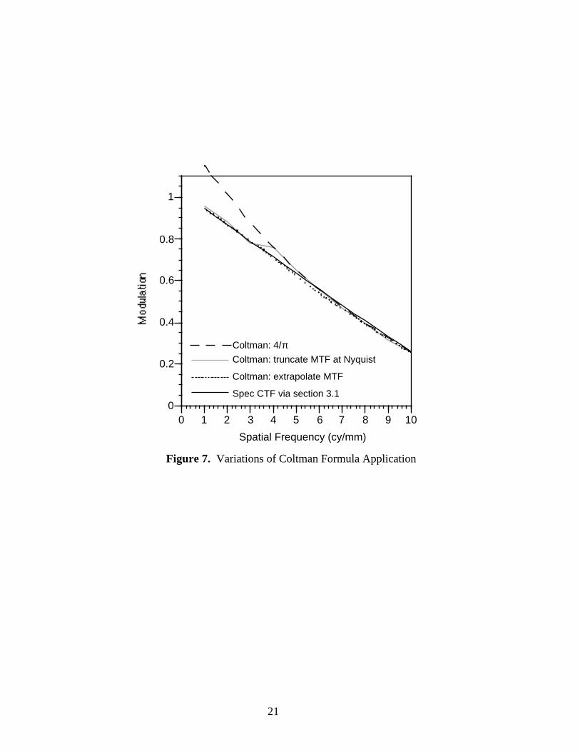
Figure 7 gives the CTF results of these three approaches when using the spec MTF at 500 ppi asthe input to the Coltman formula (Equation (11)), and compares the resulting Coltman CTFs tothe spec CTF derived via the technique described in Section 3.1. Clearly, the 4/π approach andspec-MTF-truncated-at-Nyquist approach lead to large errors at a significant number offrequencies. On the other hand, the spec-MTF-extrapolated-beyond-Nyquist approach givesresults very close to the spec CTF derived in Section 3.1.

In fact, the integration kernel in Equation (8) has similarities to the Coltman formula in Equation11, if one expands Equation (8) into a series. To illustrate this similarity, Figure 8 shows theCTF of a diffraction-limited lens (difflim) having a cutoff frequency of 10.0 cy/mm, as computedby the Coltman formula and by the method in Section 3.1. For the latter, as a further test of thecomputer program, the CTF for a 50-bar target was computed two ways, which should giveequivalent results: (1) point sampling was assumed, with a pixel width = 0.0001 mm, pixel pitch= 0.050 mm (Nyquist=10.0 cy/mm) and using difflimMTF as input, and (2) a finite pixelsampling width = 0.050 mm was assumed (Nyquist=10.0 cy/mm, pixel pitch=0.050 mm), using[difflimMTF / sinc(.05πf)] as input. As is seen in Figure 8, all three computed CTF curvesoverlap, and they also agree with published data for the CTF of a diffraction-limited lens (Bassand VanStryland, 1994).

In summary, the technique described in Section 3.1, which admittedly does involve more complexcomputations than the Coltman approach, is believed to be the more accurate approach for theapplication at hand. The Section 3.1 approach can account for a small number of target bars,whereas the Coltman formula inherently assumes an infinite number of bars. Also, the section3.1 approach is more conducive to modeling the discrete-area sampling of a sampled imagingsystem, including pixel widths that may be less than pixel pitch, whereas the Coltman formula isfundamentally for an analog, continuous imaging system.

21

Figure 7. Variations of Coltman Formula Application

0

0.2

0.4

0.6

0.8

1

0 1 2 3 4 5 6 7 8 9 10


Coltman: 4/πColtman: truncate MTF at Nyquist

Coltman: extrapolate MTF

Spec CTF via section 3.1

22

cy/mm difflimMTF(input)

Coltman CTF sec 3.1 CTF(point sampling)

sec 3.1 CTF(area sampling)

1 0.872889 0.917271 0.91875183 0.918751832 0.74706 0.830332 0.8348011 0.83480123 0.623838 0.778428 0.7798474 0.779847914 0.504632 0.642517 0.64397621 0.643977345 0.391002 0.497839 0.49920773 0.49920926 0.284757 0.362564 0.3637381 0.3637387 0.18812 0.239522 0.239309 0.24041928 0.104088 0.132529 0.133088 0.133088939 0.037386 0.04760133 0.04783677 0.04783712

10 0.000000 0.000000 0.00015346 0.00015338

Figure 8. Lens CTF Calculated via Coltman and Section 3.1 Method

0

0.1

0.2

0.3

0.4

0.5

0.6

0.7

0.8

0.9

1

0 1 2 3 4 5 6 7 8 9 10


Coltman

sec.3.1-point sampling

sec.3.1-area sampling

23

3.3 CTF Normalization

In actual computation of a scanner's CTF from a scanned bar target, the maximum imagemodulation is first determined from the highest peak and lowest valley combination found withinone period. It would often lead to a more accurate result if the peak and valley image gray levelswere first converted to their equivalent values in target space before computing image modulation,because this normalizes out gray level measurement differences between the target and scanner-produced image. Bar targets, however, are rarely fabricated with the surrounding uniform graypatches (see Figure 1) necessary to construct the conversion curve. This leaves the choice ofeither denoting the curve generated from the image modulations as the scanner CTF, ornormalizing this curve by a very low frequency modulation value and denoting the result as thescanner CTF. On the upside, the latter approach has the advantage of normalizing-out the effectof a bar target whose effective modulation, as 'seen' by the particular scanner, may be less than1.0. On the downside, the latter approach will normalize out the degrading effect of any existinglight flare or veiling glare that is a part of the scanner performance/design. Analysis of test datafrom several IQS certified scanners that used bar targets, indicate that CTF normalization by themodulation at a very low frequency (less than 5% of Nyquist) is usually possible andstraightforward, and results in a good measure of the CTF. Also, it should be noted that if thetarget bar modulations decrease with increasing frequency, and those target modulations can bemeasured, then this would be an additional normalization factor to apply to the imaging system'smeasured CTF.

25

LIST OF REFERENCES

Barakat, R. and S. Lerman, March 1967, Diffraction Images of Truncated, One-Dimensional,Periodic Targets, Applied Optics, Vol. 6, No. 3, pp. 545-548.

Bass, M. and E. W. VanStryland, editors, 1994, Handbook of Optics, chapter on: "TransferFunction Techniques" by G. D. Boreman, 2nd edition, Vol.II, New York: McGraw-Hill, pg. 32.9.

Coltman, J. W., June 1954, The Specification of Imaging Properties by Response to a Sine WaveTarget, Journal of the Optical Society of America, Vol. 44, No. 6, pp. 468-471.

FBI, March 1995, Test Procedures for Verifying IAFIS Scanner Image Quality Requirements,document number CJIS-TD-0110, Federal Bureau of Investigation, Washington, DC.

FBI, January 1999, Electronic Fingerprint Transmission Specification, Appendix F- "IAFISImage Quality Specifications (IQS)", document number CJIS-RS-0100 (V7), Federal Bureau ofInvestigation, Washington, DC.

Feltz, J. C. and M. A. Karim, February 1990, Modulation Transfer Function of Charge-CoupledDevices, Applied Optics, Vol. 29, No. 5, pp. 717–722.

MITRE Corporation, 2001, "Image Quality Evaluation" at: http://www.mitre.org/technology/mtf

Park, S. K., R. Schowengerdt, and M. Kaczynski, 1 August 1984, Modulation Transfer FunctionAnalysis for Sampled Image Systems, Applied Optics, Vol. 23, No. 15, pp. 2572–2582.

Smith, W. J., 1966, Modern Optical Engineering, Section 4.6: "Total Internal Reflection",New York: McGraw-Hill.

Tannas, L. E., editor, 1985, Flat Panel Displays and CRTs, chapter on: "Image Quality: Measuresand Visual Performance" by H. L. Snyder, New York: Van Nostrand, pp. 70–91.

http://www.mitre.org/technology/mtf

27

Appendix

Computed CTFs

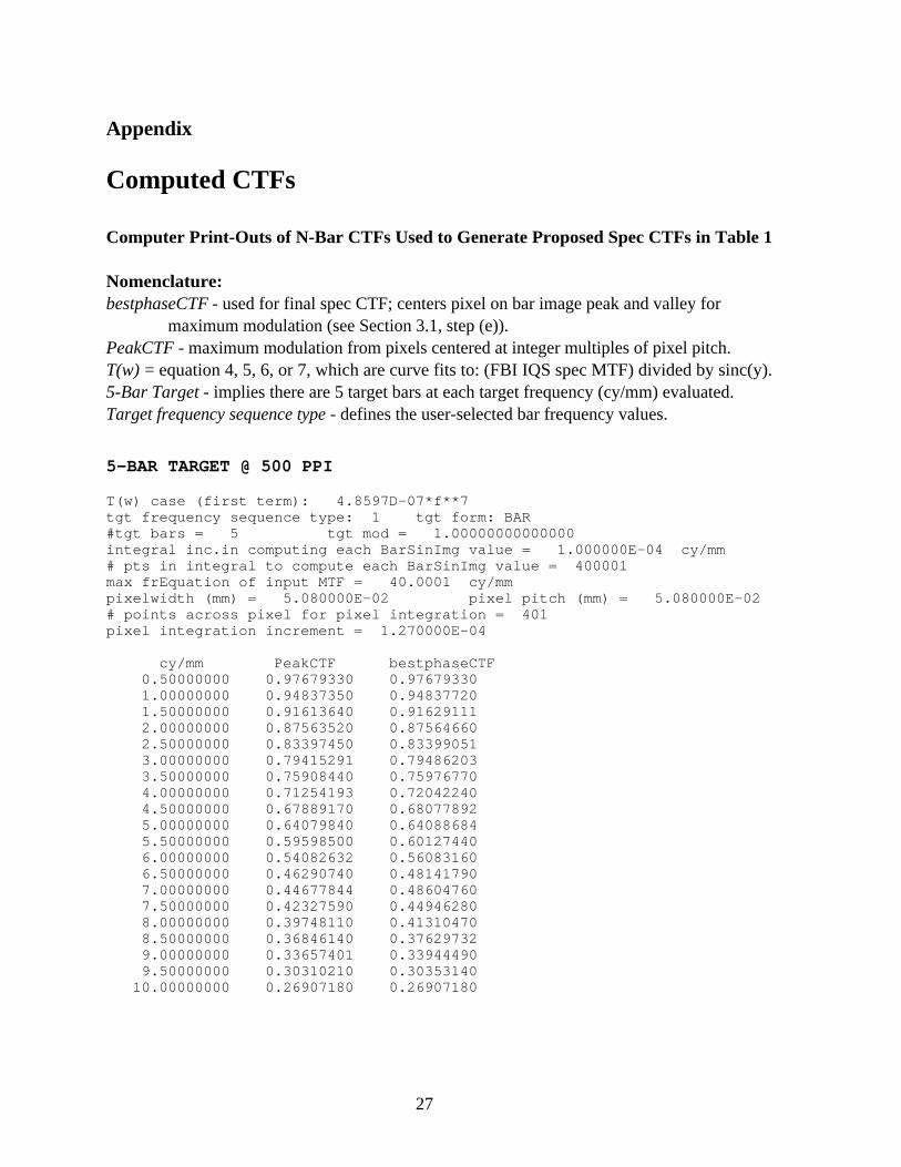
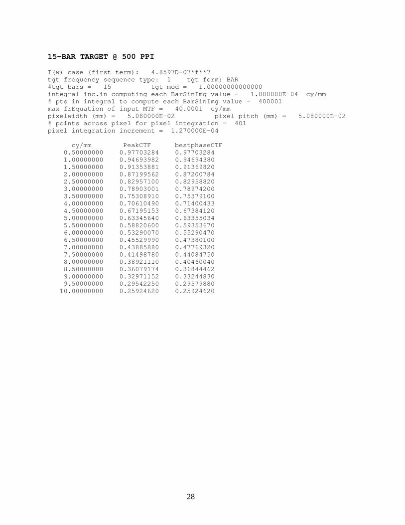
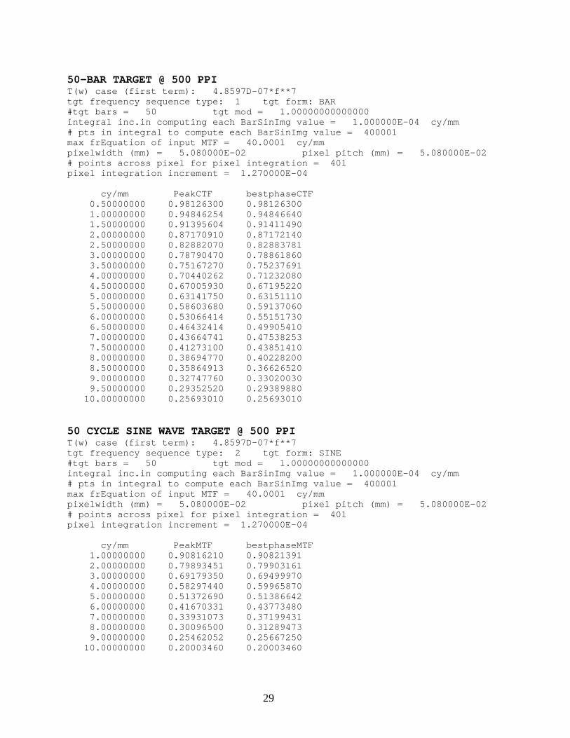
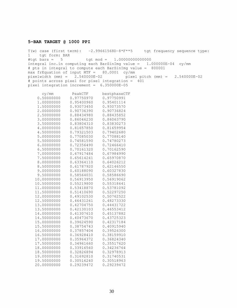
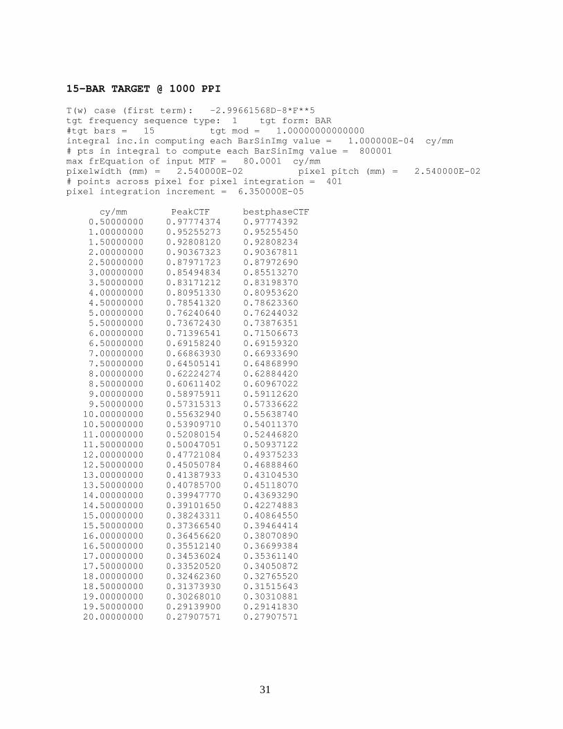
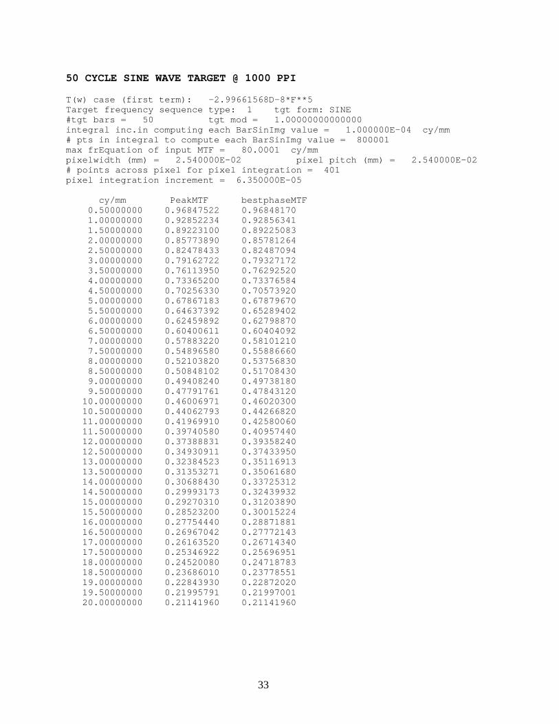
Computer Print-Outs of N-Bar CTFs Used to Generate Proposed Spec CTFs in Table 1

Nomenclature:bestphaseCTF - used for final spec CTF; centers pixel on bar image peak and valley for

maximum modulation (see Section 3.1, step (e)).PeakCTF - maximum modulation from pixels centered at integer multiples of pixel pitch.T(w) = equation 4, 5, 6, or 7, which are curve fits to: (FBI IQS spec MTF) divided by sinc(y).5-Bar Target - implies there are 5 target bars at each target frequency (cy/mm) evaluated.Target frequency sequence type - defines the user-selected bar frequency values.

5-BAR TARGET @ 500 PPI T(w) case (first term): 4.8597D-07*f**7tgt frequency sequence type: 1 tgt form: BAR#tgt bars = 5 tgt mod = 1.00000000000000integral inc.in computing each BarSinImg value = 1.000000E-04 cy/mm# pts in integral to compute each BarSinImg value = 400001max frEquation of input MTF = 40.0001 cy/mmpixelwidth (mm) = 5.080000E-02 pixel pitch (mm) = 5.080000E-02# points across pixel for pixel integration = 401pixel integration increment = 1.270000E-04

cy/mm PeakCTF bestphaseCTF 0.50000000 0.97679330 0.97679330 1.00000000 0.94837350 0.94837720 1.50000000 0.91613640 0.91629111 2.00000000 0.87563520 0.87564660 2.50000000 0.83397450 0.83399051 3.00000000 0.79415291 0.79486203 3.50000000 0.75908440 0.75976770 4.00000000 0.71254193 0.72042240 4.50000000 0.67889170 0.68077892 5.00000000 0.64079840 0.64088684 5.50000000 0.59598500 0.60127440 6.00000000 0.54082632 0.56083160 6.50000000 0.46290740 0.48141790 7.00000000 0.44677844 0.48604760 7.50000000 0.42327590 0.44946280 8.00000000 0.39748110 0.41310470 8.50000000 0.36846140 0.37629732 9.00000000 0.33657401 0.33944490 9.50000000 0.30310210 0.30353140 10.00000000 0.26907180 0.26907180

28



29



50 CYCLE SINE WAVE TARGET @ 500 PPI T(w) case (first term): 4.8597D-07*f**7tgt frequency sequence type: 2 tgt form: SINE#tgt bars = 50 tgt mod = 1.00000000000000integral inc.in computing each BarSinImg value = 1.000000E-04 cy/mm# pts in integral to compute each BarSinImg value = 400001max frEquation of input MTF = 40.0001 cy/mmpixelwidth (mm) = 5.080000E-02 pixel pitch (mm) = 5.080000E-02# points across pixel for pixel integration = 401pixel integration increment = 1.270000E-04

cy/mm PeakMTF bestphaseMTF 1.00000000 0.90816210 0.90821391 2.00000000 0.79893451 0.79903161 3.00000000 0.69179350 0.69499970 4.00000000 0.58297440 0.59965870 5.00000000 0.51372690 0.51386642 6.00000000 0.41670331 0.43773480 7.00000000 0.33931073 0.37199431 8.00000000 0.30096500 0.31289473 9.00000000 0.25462052 0.25667250 10.00000000 0.20003460 0.20003460

30

5-BAR TARGET @ 1000 PPI

T(w) case (first term): -2.99661568D-8*F**5 tgt frequency sequence type:1 tgt form: BAR#tgt bars = 5 tgt mod = 1.00000000000000integral inc.in computing each BarSinImg value = 1.000000E-04 cy/mm# pts in integral to compute each BarSinImg value = 800001max frEquation of input MTF = 80.0001 cy/mmpixelwidth (mm) = 2.540000E-02 pixel pitch (mm) = 2.540000E-02# points across pixel for pixel integration = 401pixel integration increment = 6.350000E-05

cy/mm PeakCTF bestphaseCTF 0.50000000 0.97750970 0.97750991 1.00000000 0.95400960 0.95401114 1.50000000 0.93073450 0.93073570 2.00000000 0.90736390 0.90736824 2.50000000 0.88434980 0.88435852 3.00000000 0.86046230 0.86063790 3.50000000 0.83804310 0.83830273 4.00000000 0.81657850 0.81659954 4.50000000 0.79321503 0.79402680 5.00000000 0.77085030 0.77088140 5.50000000 0.74581590 0.74780273 6.00000000 0.72356490 0.72466410 6.50000000 0.70161320 0.70162590 7.00000000 0.67917484 0.67984990 7.50000000 0.65614241 0.65970870 8.00000000 0.63364110 0.64026212 8.50000000 0.61787920 0.62146550 9.00000000 0.60188090 0.60327830 9.50000000 0.58564031 0.58586690 10.00000000 0.56913950 0.56919062 10.50000000 0.55219800 0.55318641 11.00000000 0.53418870 0.53781092 11.50000000 0.51410690 0.52297250 12.00000000 0.49102530 0.50762522 12.50000000 0.46431261 0.48273330 13.00000000 0.42704750 0.44431722 13.50000000 0.42130103 0.46553412 14.00000000 0.41307610 0.45137882 14.50000000 0.40473670 0.43725323 15.00000000 0.39624590 0.42317184 15.50000000 0.38754743 0.40915940 16.00000000 0.37857404 0.39526300 16.50000000 0.36928410 0.38159910 17.00000000 0.35964372 0.36824340 17.50000000 0.34961660 0.35517620 18.00000000 0.33916560 0.34236764 18.50000000 0.32826894 0.32978913 19.00000000 0.31692810 0.31740531 19.50000000 0.30516240 0.30518963 20.00000000 0.29239472 0.29239472

31

15-BAR TARGET @ 1000 PPI T(w) case (first term): -2.99661568D-8*F**5tgt frequency sequence type: 1 tgt form: BAR#tgt bars = 15 tgt mod = 1.00000000000000integral inc.in computing each BarSinImg value = 1.000000E-04 cy/mm# pts in integral to compute each BarSinImg value = 800001max frEquation of input MTF = 80.0001 cy/mmpixelwidth (mm) = 2.540000E-02 pixel pitch (mm) = 2.540000E-02# points across pixel for pixel integration = 401pixel integration increment = 6.350000E-05


32

50-BAR TARGET @ 1000 PPI T(w) case (first term): -2.99661568D-8*F**5tgt frequency sequence type: 1 tgt form: BAR#tgt bars = 50 tgt mod = 1.00000000000000integral inc.in computing each BarSinImg value = 1.000000E-04 cy/mm# pts in integral to compute each BarSinImg value = 800001max frEquation of input MTF = 80.0001 cy/mmpixelwidth (mm) = 2.540000E-02 pixel pitch (mm) = 2.540000E-02# points across pixel for pixel integration = 401pixel integration increment = 6.350000E-05


33

50 CYCLE SINE WAVE TARGET @ 1000 PPI

T(w) case (first term): -2.99661568D-8*F**5Target frequency sequence type: 1 tgt form: SINE#tgt bars = 50 tgt mod = 1.00000000000000integral inc.in computing each BarSinImg value = 1.000000E-04 cy/mm# pts in integral to compute each BarSinImg value = 800001max frEquation of input MTF = 80.0001 cy/mmpixelwidth (mm) = 2.540000E-02 pixel pitch (mm) = 2.540000E-02# points across pixel for pixel integration = 401pixel integration increment = 6.350000E-05

cy/mm PeakMTF bestphaseMTF 0.50000000 0.96847522 0.96848170 1.00000000 0.92852234 0.92856341 1.50000000 0.89223100 0.89225083 2.00000000 0.85773890 0.85781264 2.50000000 0.82478433 0.82487094 3.00000000 0.79162722 0.79327172 3.50000000 0.76113950 0.76292520 4.00000000 0.73365200 0.73376584 4.50000000 0.70256330 0.70573920 5.00000000 0.67867183 0.67879670 5.50000000 0.64637392 0.65289402 6.00000000 0.62459892 0.62798870 6.50000000 0.60400611 0.60404092 7.00000000 0.57883220 0.58101210 7.50000000 0.54896580 0.55886660 8.00000000 0.52103820 0.53756830 8.50000000 0.50848102 0.51708430 9.00000000 0.49408240 0.49738180 9.50000000 0.47791761 0.47843120 10.00000000 0.46006971 0.46020300 10.50000000 0.44062793 0.44266820 11.00000000 0.41969910 0.42580060 11.50000000 0.39740580 0.40957440 12.00000000 0.37388831 0.39358240 12.50000000 0.34930911 0.37433950 13.00000000 0.32384523 0.35116913 13.50000000 0.31353271 0.35061680 14.00000000 0.30688430 0.33725312 14.50000000 0.29993173 0.32439932 15.00000000 0.29270310 0.31203890 15.50000000 0.28523200 0.30015224 16.00000000 0.27754440 0.28871881 16.50000000 0.26967042 0.27772143 17.00000000 0.26163520 0.26714340 17.50000000 0.25346922 0.25696951 18.00000000 0.24520080 0.24718783 18.50000000 0.23686010 0.23778551 19.00000000 0.22843930 0.22872020 19.50000000 0.21995791 0.21997001 20.00000000 0.21141960 0.21141960

35

GLOSSARY

ANSI American National Standards Institute

avg average

CCD Charge-Coupled Device

COTS Commercial Off-The-Shelf

CTF Contrast Transfer Function

cy/mm cycles per millimeter

FBI Federal Bureau of Investigation

IAFIS Integrated Automated Fingerprint Identification System

I/O Input / Output

IQS Image Quality Specification

ISO International Organization of Standardization

mm millimeter

MTF Modulation Transfer Function

NBS National Bureau of Standards

ppi pixels per inch

sinemtf MITRE's computer program to compute the sine wave MTF or square wave CTF

tgt target

USAF United States Air Force

conversion between sine wave and square wave spatial ...conversion between sine wave and square wave...

Documents