convex optimization for big data - ubc computer science · convex functionssmooth...
TRANSCRIPT

Convex Functions Smooth Optimization Non-Smooth Optimization Randomized Algorithms Parallel/Distributed Optimization
Convex Optimization for Big DataAsian Conference on Machine Learning
Mark Schmidt
November 2014
Convex Functions Smooth Optimization Non-Smooth Optimization Randomized Algorithms Parallel/Distributed Optimization
Context: Big Data and Big Models
We are collecting data at unprecedented rates.
Seen across many fields of science and engineering.Not gigabytes, but terabytes or petabytes (and beyond).
Many important aspects to the ‘big data’ puzzle:
Distributed data storage and management, parallelcomputation, software paradigms, data mining, machinelearning, privacy and security issues, reacting to other agents,power management, summarization and visualization.
Convex Functions Smooth Optimization Non-Smooth Optimization Randomized Algorithms Parallel/Distributed Optimization
Context: Big Data and Big Models
Machine learning uses big data to fit richer statistical models:
Vision, bioinformatics, speech, natural language, web, social.Developping broadly applicable tools.Output of models can be used for further analysis.
Numerical optimization is at the core of many of these models.
But, traditional ‘black-box’ methods have difficulty with:
the large data sizes.the large model complexities.
Convex Functions Smooth Optimization Non-Smooth Optimization Randomized Algorithms Parallel/Distributed Optimization
Motivation: Why Learn about Convex Optimization?
Why learn about optimization?
Optimization is at the core of many ML algorithms.
ML is driving a lot of modern research in optimization.
Why in particular learn about convex optimization?
Among only efficiently-solvable continuous problems.
You can do a lot with convex models.(least squares, lasso, generlized linear models, SVMs, CRFs)
Empirically effective non-convex methods are often basedmethods with good properties for convex objectives.
(functions are locally convex around minimizers)

Convex Functions Smooth Optimization Non-Smooth Optimization Randomized Algorithms Parallel/Distributed Optimization
Two Components of My Research
The first component of my research focuses on computation:
We ‘open up the black box’, by using the structure of machinemodels to derive faster large-scale optimization algorithms.Can lead to enormous speedups for big data and complexmodels.
The second component of my research focuses on modeling:
By expanding the set of tractable problems, we can proposericher classes of statistical models that can be efficiently fit.
We can alternate between these two.

Convex Functions Smooth Optimization Non-Smooth Optimization Randomized Algorithms Parallel/Distributed Optimization
Outline
1 Convex Functions
2 Smooth Optimization
3 Non-Smooth Optimization
4 Randomized Algorithms
5 Parallel/Distributed Optimization

Convex Functions Smooth Optimization Non-Smooth Optimization Randomized Algorithms Parallel/Distributed Optimization
Convexity: Zero-order condition
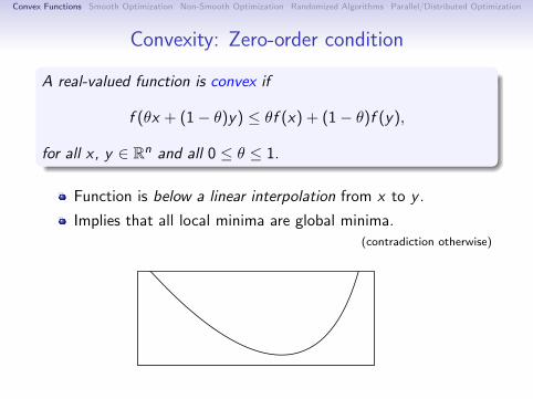
A real-valued function is convex if
f (θx + (1− θ)y) ≤ θf (x) + (1− θ)f (y),
for all x , y ∈ Rn and all 0 ≤ θ ≤ 1.
Function is below a linear interpolation from x to y .
Implies that all local minima are global minima.(contradiction otherwise)
Convex Functions Smooth Optimization Non-Smooth Optimization Randomized Algorithms Parallel/Distributed Optimization
Convexity: Zero-order condition
A real-valued function is convex if
f (θx + (1− θ)y) ≤ θf (x) + (1− θ)f (y),
for all x , y ∈ Rn and all 0 ≤ θ ≤ 1.
Function is below a linear interpolation from x to y .
Implies that all local minima are global minima.(contradiction otherwise)
f(x)
f(y)
0.5f(x) + 0.5f(y)
f(0.5x + 0.5y)

Convex Functions Smooth Optimization Non-Smooth Optimization Randomized Algorithms Parallel/Distributed Optimization
Convexity: Zero-order condition
A real-valued function is convex if
f (θx + (1− θ)y) ≤ θf (x) + (1− θ)f (y),
for all x , y ∈ Rn and all 0 ≤ θ ≤ 1.
Function is below a linear interpolation from x to y .
Implies that all local minima are global minima.(contradiction otherwise)
Not convex

Convex Functions Smooth Optimization Non-Smooth Optimization Randomized Algorithms Parallel/Distributed Optimization
Convexity: Zero-order condition
A real-valued function is convex if
f (θx + (1− θ)y) ≤ θf (x) + (1− θ)f (y),
for all x , y ∈ Rn and all 0 ≤ θ ≤ 1.
Function is below a linear interpolation from x to y .
Implies that all local minima are global minima.(contradiction otherwise)
f(x)f(y)
Not convexNon-global
local minima

Convex Functions Smooth Optimization Non-Smooth Optimization Randomized Algorithms Parallel/Distributed Optimization
Convexity of Norms
We say that a function f is a norm if:
1 f (0) = 0.
2 f (θx) = |θ|f (x).
3 f (x + y) ≤ f (x) + f (y).
Examples:
‖x‖2 =
√∑
i
x2i =√xT x
‖x‖1 =∑
i
|xi |
‖x‖H =√xTHx
Norms are convex:
f (θx + (1− θ)y) ≤ f (θx) + f ((1− θ)y) (3)
= θf (x) + (1− θ)f (y) (2)
Convex Functions Smooth Optimization Non-Smooth Optimization Randomized Algorithms Parallel/Distributed Optimization
Strict Convexity
A real-valued function is strictly convex if
f (θx + (1− θ)y) < θf (x) + (1− θ)f (y),
for all x 6= y ∈ Rn and all 0 < θ < 1.
Strictly below the linear interpolation from x to y .
Implies at most one global minimum.(otherwise, could construct lower global minimum)

Convex Functions Smooth Optimization Non-Smooth Optimization Randomized Algorithms Parallel/Distributed Optimization
Convexity: First-order condition
A real-valued differentiable function is convex iff
f (y) ≥ f (x) +∇f (x)T (y − x),
for all x , y ∈ Rn.
The function is globally above the tangent at x .(if ∇f (y) = 0 then y is a a global minimizer)
f(x)
f(x) + ∇f(x)T(y-x)
f(y)

Convex Functions Smooth Optimization Non-Smooth Optimization Randomized Algorithms Parallel/Distributed Optimization
Convexity: Second-order condition
A real-valued twice-differentiable function is convex iff
∇2f (x) 0
for all x ∈ Rn.
The function is flat or curved upwards in every direction.
A real-valued function f is a quadratic if it can be written in theform:
f (x) =1
2xTAx + bT x + c .
Since ∇2f (x) = A, it is convex if A 0.E.g., least squares has ∇2f (x) = ATA 0.

Convex Functions Smooth Optimization Non-Smooth Optimization Randomized Algorithms Parallel/Distributed Optimization
Examples of Convex Functions
Some simple convex functions:
f (x) = c
f (x) = aT x
f (x) = ax2 + b (for a > 0)
f (x) = exp(ax)
f (x) = x log x (for x > 0)
f (x) = ||x ||2f (x) = maxixi
Some other notable examples:
f (x , y) = log(ex + ey )
f (X ) = log detX (for X positive-definite).
f (x ,Y ) = xTY−1x (for Y positive-definite)

Convex Functions Smooth Optimization Non-Smooth Optimization Randomized Algorithms Parallel/Distributed Optimization
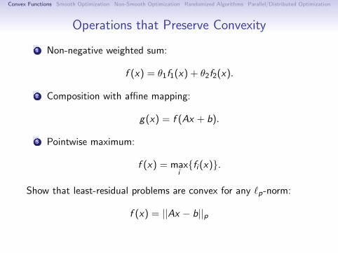
Operations that Preserve Convexity
1 Non-negative weighted sum:
f (x) = θ1f1(x) + θ2f2(x).
2 Composition with affine mapping:
g(x) = f (Ax + b).
3 Pointwise maximum:
f (x) = maxifi (x).
Show that least-residual problems are convex for any `p-norm:
f (x) = ||Ax − b||p
We know that ‖ · ‖p is a norm, so it follows from (2).
Convex Functions Smooth Optimization Non-Smooth Optimization Randomized Algorithms Parallel/Distributed Optimization
Operations that Preserve Convexity
1 Non-negative weighted sum:
f (x) = θ1f1(x) + θ2f2(x).
2 Composition with affine mapping:
g(x) = f (Ax + b).
3 Pointwise maximum:
f (x) = maxifi (x).
Show that least-residual problems are convex for any `p-norm:
f (x) = ||Ax − b||p
We know that ‖ · ‖p is a norm, so it follows from (2).

Convex Functions Smooth Optimization Non-Smooth Optimization Randomized Algorithms Parallel/Distributed Optimization
Operations that Preserve Convexity
1 Non-negative weighted sum:
f (x) = θ1f1(x) + θ2f2(x).
2 Composition with affine mapping:
g(x) = f (Ax + b).
3 Pointwise maximum:
f (x) = maxifi (x).
Show that SVMs are convex:
f (x) =1
2||x ||2 + C
n∑
i=1
max0, 1− biaTi x.
The first term has Hessian I 0, for the second term use (3) onthe two (convex) arguments, then use (1) to put it all together.
Convex Functions Smooth Optimization Non-Smooth Optimization Randomized Algorithms Parallel/Distributed Optimization
Outline
1 Convex Functions
2 Smooth Optimization
3 Non-Smooth Optimization
4 Randomized Algorithms
5 Parallel/Distributed Optimization

Convex Functions Smooth Optimization Non-Smooth Optimization Randomized Algorithms Parallel/Distributed Optimization
How hard is real-valued optimization?How long to find an ε-optimal minimizer of a real-valued function?
minx∈Rn
f (x).
General function: impossible!(think about arbitrarily small value at some infinite decimal expansion)
We need to make some assumptions about the function:
Assume f is Lipschitz-continuous: (can not change too quickly)
|f (x)− f (y)| ≤ L‖x − y‖.

Convex Functions Smooth Optimization Non-Smooth Optimization Randomized Algorithms Parallel/Distributed Optimization
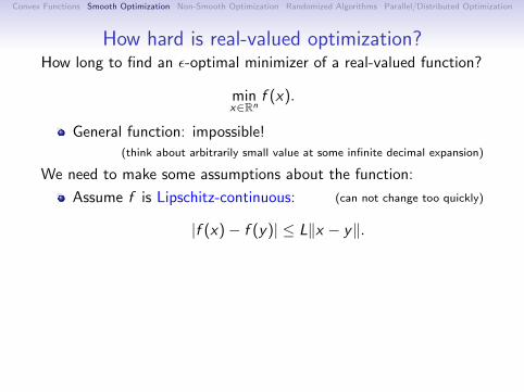
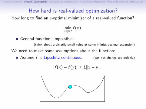
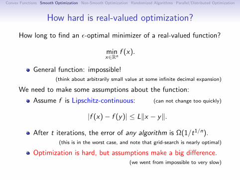
How hard is real-valued optimization?
How long to find an ε-optimal minimizer of a real-valued function?
minx∈Rn
f (x).
General function: impossible!(think about arbitrarily small value at some infinite decimal expansion)
We need to make some assumptions about the function:
Assume f is Lipschitz-continuous: (can not change too quickly)
|f (x)− f (y)| ≤ L‖x − y‖.
After t iterations, the error of any algorithm is Ω(1/t1/n).(this is in the worst case, and note that grid-search is nearly optimal)
Optimization is hard, but assumptions make a big difference.(we went from impossible to very slow)
Convex Functions Smooth Optimization Non-Smooth Optimization Randomized Algorithms Parallel/Distributed Optimization
How hard is real-valued optimization?
How long to find an ε-optimal minimizer of a real-valued function?
minx∈Rn
f (x).
General function: impossible!(think about arbitrarily small value at some infinite decimal expansion)
We need to make some assumptions about the function:
Assume f is Lipschitz-continuous: (can not change too quickly)
|f (x)− f (y)| ≤ L‖x − y‖.
After t iterations, the error of any algorithm is Ω(1/t1/n).(this is in the worst case, and note that grid-search is nearly optimal)
Optimization is hard, but assumptions make a big difference.(we went from impossible to very slow)

Convex Functions Smooth Optimization Non-Smooth Optimization Randomized Algorithms Parallel/Distributed Optimization
Motivation for First-Order Methods
Well-known that we can solve convex optimization problemsin polynomial-time by interior-point methods
However, these solvers require O(n2) or worse cost periteration.
Infeasible for applications where n may be in the billions.
Solving big problems has led to re-newed interest in simplefirst-order methods (gradient methods):
x+ = x − α∇f (x).
These only have O(n) iteration costs.But we must analyze how many iterations are needed.
Convex Functions Smooth Optimization Non-Smooth Optimization Randomized Algorithms Parallel/Distributed Optimization
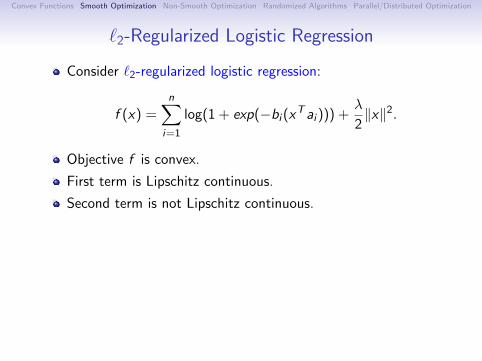
`2-Regularized Logistic Regression
Consider `2-regularized logistic regression:
f (x) =n∑
i=1
log(1 + exp(−bi (xTai ))) +λ
2‖x‖2.
Objective f is convex.
First term is Lipschitz continuous.
Second term is not Lipschitz continuous.
But we haveµI ∇2f (x) LI .
(L = 14‖A‖2
2 + λ, µ = λ)
Gradient is Lipschitz-continuous.
Function is strongly-convex.(implies strict convexity, and existence of unique solution)

Convex Functions Smooth Optimization Non-Smooth Optimization Randomized Algorithms Parallel/Distributed Optimization
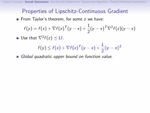
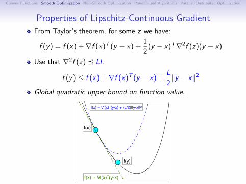
Properties of Lipschitz-Continuous GradientFrom Taylor’s theorem, for some z we have:
f (y) = f (x) +∇f (x)T (y − x) +1
2(y − x)T∇2f (z)(y − x)
Use that ∇2f (z) LI .
f (y) ≤ f (x) +∇f (x)T (y − x) +L
2‖y − x‖2
Global quadratic upper bound on function value.
Convex Functions Smooth Optimization Non-Smooth Optimization Randomized Algorithms Parallel/Distributed Optimization
Properties of Lipschitz-Continuous GradientFrom Taylor’s theorem, for some z we have:
f (y) = f (x) +∇f (x)T (y − x) +1
2(y − x)T∇2f (z)(y − x)
Use that ∇2f (z) LI .
f (y) ≤ f (x) +∇f (x)T (y − x) +L
2‖y − x‖2
Global quadratic upper bound on function value.
f(x)

Convex Functions Smooth Optimization Non-Smooth Optimization Randomized Algorithms Parallel/Distributed Optimization
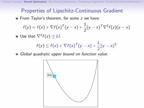
Properties of Lipschitz-Continuous GradientFrom Taylor’s theorem, for some z we have:
f (y) = f (x) +∇f (x)T (y − x) +1
2(y − x)T∇2f (z)(y − x)
Use that ∇2f (z) LI .
f (y) ≤ f (x) +∇f (x)T (y − x) +L
2‖y − x‖2
Global quadratic upper bound on function value.
f(x)
f(x) + ∇f(x)T(y-x)

Convex Functions Smooth Optimization Non-Smooth Optimization Randomized Algorithms Parallel/Distributed Optimization
Properties of Lipschitz-Continuous GradientFrom Taylor’s theorem, for some z we have:
f (y) = f (x) +∇f (x)T (y − x) +1
2(y − x)T∇2f (z)(y − x)
Use that ∇2f (z) LI .
f (y) ≤ f (x) +∇f (x)T (y − x) +L
2‖y − x‖2
Global quadratic upper bound on function value.
f(x)
f(x) + ∇f(x)T(y-x)
f(x) + ∇f(x)T(y-x) + (L/2)||y-x||2
Convex Functions Smooth Optimization Non-Smooth Optimization Randomized Algorithms Parallel/Distributed Optimization
Properties of Lipschitz-Continuous GradientFrom Taylor’s theorem, for some z we have:
f (y) = f (x) +∇f (x)T (y − x) +1
2(y − x)T∇2f (z)(y − x)
Use that ∇2f (z) LI .
f (y) ≤ f (x) +∇f (x)T (y − x) +L
2‖y − x‖2
Global quadratic upper bound on function value.
f(x)
f(x) + ∇f(x)T(y-x)
f(y)
f(x) + ∇f(x)T(y-x) + (L/2)||y-x||2

Convex Functions Smooth Optimization Non-Smooth Optimization Randomized Algorithms Parallel/Distributed Optimization
Properties of Lipschitz-Continuous GradientFrom Taylor’s theorem, for some z we have:
f (y) = f (x) +∇f (x)T (y − x) +1
2(y − x)T∇2f (z)(y − x)
Use that ∇2f (z) LI .
f (y) ≤ f (x) +∇f (x)T (y − x) +L
2‖y − x‖2
Global quadratic upper bound on function value.
Stochastic vs. deterministic methods
• Minimizing g(!) =1
n
n!
i=1
fi(!) with fi(!) = ""yi, !
!!(xi)#
+ µ"(!)
• Batch gradient descent: !t = !t"1!#tg#(!t"1) = !t"1!
#t
n
n!
i=1
f #i(!t"1)
• Stochastic gradient descent: !t = !t"1 ! #tf#i(t)(!t"1)

Convex Functions Smooth Optimization Non-Smooth Optimization Randomized Algorithms Parallel/Distributed Optimization
Properties of Lipschitz-Continuous Gradient
From Taylor’s theorem, for some z we have:
f (y) = f (x) +∇f (x)T (y − x) +1
2(y − x)T∇2f (z)(y − x)
Use that ∇2f (z) LI .
f (y) ≤ f (x) +∇f (x)T (y − x) +L
2‖y − x‖2
Global quadratic upper bound on function value.
Set x+ to minimize upper bound in terms of y :
x+ = x − 1
L∇f (x).
(gradient descent with step-size of 1/L)
Plugging this value in:
f (x+) ≤ f (x)− 1
2L‖∇f (x)‖2.
(decrease of at least 12L‖∇f (x)‖2)
Convex Functions Smooth Optimization Non-Smooth Optimization Randomized Algorithms Parallel/Distributed Optimization
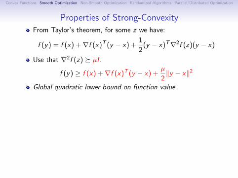
Properties of Strong-ConvexityFrom Taylor’s theorem, for some z we have:
f (y) = f (x) +∇f (x)T (y − x) +1
2(y − x)T∇2f (z)(y − x)
Use that ∇2f (z) µI .f (y) ≥ f (x) +∇f (x)T (y − x) +
µ
2‖y − x‖2
Global quadratic lower bound on function value.
Convex Functions Smooth Optimization Non-Smooth Optimization Randomized Algorithms Parallel/Distributed Optimization
Properties of Strong-ConvexityFrom Taylor’s theorem, for some z we have:
f (y) = f (x) +∇f (x)T (y − x) +1
2(y − x)T∇2f (z)(y − x)
Use that ∇2f (z) µI .f (y) ≥ f (x) +∇f (x)T (y − x) +
µ
2‖y − x‖2
Global quadratic lower bound on function value.
f(x)
f(x) + ∇f(x)T(y-x)
f(x) + ∇f(x)T(y-x) + (μ/2)||y-x||2

Convex Functions Smooth Optimization Non-Smooth Optimization Randomized Algorithms Parallel/Distributed Optimization
Properties of Strong-Convexity
From Taylor’s theorem, for some z we have:
f (y) = f (x) +∇f (x)T (y − x) +1
2(y − x)T∇2f (z)(y − x)
Use that ∇2f (z) µI .
f (y) ≥ f (x) +∇f (x)T (y − x) +µ
2‖y − x‖2
Global quadratic lower bound on function value.
Minimize both sides in terms of y :
f (x∗) ≥ f (x)− 1
2µ‖∇f (x)‖2.
Upper bound on how far we are from the solution.

Convex Functions Smooth Optimization Non-Smooth Optimization Randomized Algorithms Parallel/Distributed Optimization
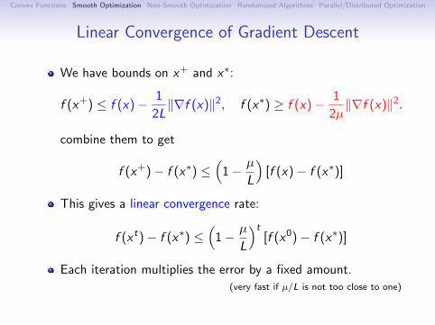
Linear Convergence of Gradient Descent
We have bounds on x+ and x∗:
f (x+) ≤ f (x)− 1
2L‖∇f (x)‖2, f (x∗) ≥ f (x)− 1
2µ‖∇f (x)‖2.

Convex Functions Smooth Optimization Non-Smooth Optimization Randomized Algorithms Parallel/Distributed Optimization
Linear Convergence of Gradient Descent
We have bounds on x+ and x∗:
f (x+) ≤ f (x)− 1
2L‖∇f (x)‖2, f (x∗) ≥ f (x)− 1
2µ‖∇f (x)‖2.
f(x)

Convex Functions Smooth Optimization Non-Smooth Optimization Randomized Algorithms Parallel/Distributed Optimization
Linear Convergence of Gradient Descent
We have bounds on x+ and x∗:
f (x+) ≤ f (x)− 1
2L‖∇f (x)‖2, f (x∗) ≥ f (x)− 1
2µ‖∇f (x)‖2.
f(x) GuaranteedProgress

Convex Functions Smooth Optimization Non-Smooth Optimization Randomized Algorithms Parallel/Distributed Optimization
Linear Convergence of Gradient Descent
We have bounds on x+ and x∗:
f (x+) ≤ f (x)− 1
2L‖∇f (x)‖2, f (x∗) ≥ f (x)− 1
2µ‖∇f (x)‖2.
f(x) GuaranteedProgress

Convex Functions Smooth Optimization Non-Smooth Optimization Randomized Algorithms Parallel/Distributed Optimization
Linear Convergence of Gradient Descent
We have bounds on x+ and x∗:
f (x+) ≤ f (x)− 1
2L‖∇f (x)‖2, f (x∗) ≥ f (x)− 1
2µ‖∇f (x)‖2.
f(x) GuaranteedProgress
MaximumSuboptimality

Convex Functions Smooth Optimization Non-Smooth Optimization Randomized Algorithms Parallel/Distributed Optimization
Linear Convergence of Gradient Descent
We have bounds on x+ and x∗:
f (x+) ≤ f (x)− 1
2L‖∇f (x)‖2, f (x∗) ≥ f (x)− 1
2µ‖∇f (x)‖2.
f(x) GuaranteedProgress
MaximumSuboptimality
f(x+)

Convex Functions Smooth Optimization Non-Smooth Optimization Randomized Algorithms Parallel/Distributed Optimization
Linear Convergence of Gradient Descent
We have bounds on x+ and x∗:
f (x+) ≤ f (x)− 1
2L‖∇f (x)‖2, f (x∗) ≥ f (x)− 1
2µ‖∇f (x)‖2.
combine them to get
f (x+)− f (x∗) ≤(
1− µ
L
)[f (x)− f (x∗)]
This gives a linear convergence rate:
f (x t)− f (x∗) ≤(
1− µ
L
)t[f (x0)− f (x∗)]
Each iteration multiplies the error by a fixed amount.(very fast if µ/L is not too close to one)

Convex Functions Smooth Optimization Non-Smooth Optimization Randomized Algorithms Parallel/Distributed Optimization
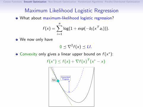
Maximum Likelihood Logistic RegressionWhat about maximum-likelihood logistic regression?
f (x) =n∑
i=1
log(1 + exp(−bi (xTai ))).
We now only have
0 ∇2f (x) LI .
Convexity only gives a linear upper bound on f (x∗):
f (x∗) ≤ f (x) +∇f (x)T (x∗ − x)

Convex Functions Smooth Optimization Non-Smooth Optimization Randomized Algorithms Parallel/Distributed Optimization
Maximum Likelihood Logistic RegressionWhat about maximum-likelihood logistic regression?
f (x) =n∑
i=1
log(1 + exp(−bi (xTai ))).
We now only have
0 ∇2f (x) LI .
Convexity only gives a linear upper bound on f (x∗):
f (x∗) ≤ f (x) +∇f (x)T (x∗ − x)
f(x)GuaranteedProgress
MaximumSuboptimality

Convex Functions Smooth Optimization Non-Smooth Optimization Randomized Algorithms Parallel/Distributed Optimization
Maximum Likelihood Logistic Regression
Consider maximum-likelihood logistic regression:
f (x) =n∑
i=1
log(1 + exp(−bi (xTai ))).
We now only have
0 ∇2f (x) LI .
Convexity only gives a linear upper bound on f (x∗):
f (x∗) ≤ f (x) +∇f (x)T (x∗ − x)
If some x∗ exists, we have the sublinear convergence rate:
f (x t)− f (x∗) = O(1/t)
(compare to slower Ω(1/t−1/N) for general Lipschitz functions)
If f is convex, then f + λ‖x‖2 is strongly-convex.

Convex Functions Smooth Optimization Non-Smooth Optimization Randomized Algorithms Parallel/Distributed Optimization
Gradient Method: Practical IssuesIn practice, searching for step size (line-search) is usuallymuch faster than α = 1/L.
(and doesn’t require knowledge of L)
Basic Armijo backtracking line-search:1 Start with a large value of α.2 Divide α in half until we satisfy (typically value is γ = .0001)
f (x+) ≤ f (x)− γα||∇f (x)||2.Practical methods may use Wolfe conditions (so α isn’t toosmall), and/or use interpolation to propose trial step sizes.
(with good interpolation, ≈ 1 evaluation of f per iteration)
Also, check your derivative code!
∇i f (x) ≈ f (x + δei )− f (x)
δFor large-scale problems you can check a random direction d :
∇f (x)Td ≈ f (x + δd)− f (x)
δ

Convex Functions Smooth Optimization Non-Smooth Optimization Randomized Algorithms Parallel/Distributed Optimization
Gradient Method: Practical IssuesIn practice, searching for step size (line-search) is usuallymuch faster than α = 1/L.
(and doesn’t require knowledge of L)
Basic Armijo backtracking line-search:1 Start with a large value of α.2 Divide α in half until we satisfy (typically value is γ = .0001)
f (x+) ≤ f (x)− γα||∇f (x)||2.
Practical methods may use Wolfe conditions (so α isn’t toosmall), and/or use interpolation to propose trial step sizes.
(with good interpolation, ≈ 1 evaluation of f per iteration)
Also, check your derivative code!
∇i f (x) ≈ f (x + δei )− f (x)
δFor large-scale problems you can check a random direction d :
∇f (x)Td ≈ f (x + δd)− f (x)
δ

Convex Functions Smooth Optimization Non-Smooth Optimization Randomized Algorithms Parallel/Distributed Optimization
Gradient Method: Practical IssuesIn practice, searching for step size (line-search) is usuallymuch faster than α = 1/L.
(and doesn’t require knowledge of L)
Basic Armijo backtracking line-search:1 Start with a large value of α.2 Divide α in half until we satisfy (typically value is γ = .0001)
f (x+) ≤ f (x)− γα||∇f (x)||2.Practical methods may use Wolfe conditions (so α isn’t toosmall), and/or use interpolation to propose trial step sizes.
(with good interpolation, ≈ 1 evaluation of f per iteration)
Also, check your derivative code!
∇i f (x) ≈ f (x + δei )− f (x)
δFor large-scale problems you can check a random direction d :
∇f (x)Td ≈ f (x + δd)− f (x)
δ

Convex Functions Smooth Optimization Non-Smooth Optimization Randomized Algorithms Parallel/Distributed Optimization
Gradient Method: Practical IssuesIn practice, searching for step size (line-search) is usuallymuch faster than α = 1/L.
(and doesn’t require knowledge of L)
Basic Armijo backtracking line-search:1 Start with a large value of α.2 Divide α in half until we satisfy (typically value is γ = .0001)
f (x+) ≤ f (x)− γα||∇f (x)||2.Practical methods may use Wolfe conditions (so α isn’t toosmall), and/or use interpolation to propose trial step sizes.
(with good interpolation, ≈ 1 evaluation of f per iteration)
Also, check your derivative code!
∇i f (x) ≈ f (x + δei )− f (x)
δFor large-scale problems you can check a random direction d :
∇f (x)Td ≈ f (x + δd)− f (x)
δ
Convex Functions Smooth Optimization Non-Smooth Optimization Randomized Algorithms Parallel/Distributed Optimization
Convergence Rate of Gradient Method
We are going to explore the ‘convex optimization zoo’:
Gradient method for smooth/convex: O(1/t).
Gradient method for smooth/strongly-convex: O((1− µ/L)t).
Rates are the same if only once-differentiable.
Line-search doesn’t change the worst-case rate.(strongly-convex slightly improved with α = 2/(µ+ L))
Is this the best algorithm under these assumptions?

Convex Functions Smooth Optimization Non-Smooth Optimization Randomized Algorithms Parallel/Distributed Optimization
Accelerated Gradient Method
Nesterov’s accelerated gradient method:
xt+1 = yt − αt∇f (yt),
yt+1 = xt + βt(xt+1 − xt),
for appropriate αt , βt .
Motivation: “to make the math work”(but similar to heavy-ball/momentum and conjugate gradient method)

Convex Functions Smooth Optimization Non-Smooth Optimization Randomized Algorithms Parallel/Distributed Optimization
Convex Optimization Zoo
Algorithm Assumptions Rate
Gradient Convex O(1/t)Nesterov Convex O(1/t2)Gradient Strongly-Convex O((1− µ/L)t)
Nesterov Strongly-Convex O((1−√µ/L)t)
O(1/t2) is optimal given only these assumptions.(sometimes called the optimal gradient method)
The faster linear convergence rate is close to optimal.
Also faster in practice, but implementation details matter.

Convex Functions Smooth Optimization Non-Smooth Optimization Randomized Algorithms Parallel/Distributed Optimization
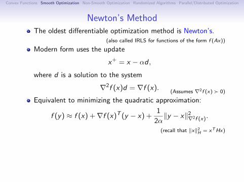
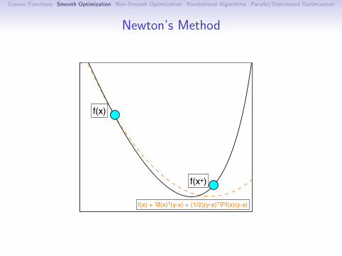
Newton’s Method
The oldest differentiable optimization method is Newton’s.(also called IRLS for functions of the form f (Ax))
Modern form uses the update
x+ = x − αd ,where d is a solution to the system
∇2f (x)d = ∇f (x).(Assumes ∇2f (x) 0)
Equivalent to minimizing the quadratic approximation:
f (y) ≈ f (x) +∇f (x)T (y − x) +1
2α‖y − x‖2
∇2f (x).
(recall that ‖x‖2H = xTHx)
We can generalize the Armijo condition to
f (x+) ≤ f (x) + γα∇f (x)Td .
Has a natural step length of α = 1.(always accepted when close to a minimizer)
Convex Functions Smooth Optimization Non-Smooth Optimization Randomized Algorithms Parallel/Distributed Optimization
Newton’s Method
The oldest differentiable optimization method is Newton’s.(also called IRLS for functions of the form f (Ax))
Modern form uses the update
x+ = x − αd ,where d is a solution to the system
∇2f (x)d = ∇f (x).(Assumes ∇2f (x) 0)
Equivalent to minimizing the quadratic approximation:
f (y) ≈ f (x) +∇f (x)T (y − x) +1
2α‖y − x‖2
∇2f (x).
(recall that ‖x‖2H = xTHx)
We can generalize the Armijo condition to
f (x+) ≤ f (x) + γα∇f (x)Td .
Has a natural step length of α = 1.(always accepted when close to a minimizer)

Convex Functions Smooth Optimization Non-Smooth Optimization Randomized Algorithms Parallel/Distributed Optimization
Newton’s Method
f(x)

Convex Functions Smooth Optimization Non-Smooth Optimization Randomized Algorithms Parallel/Distributed Optimization
Newton’s Method
f(x)
f(x) + ∇f(x)T(y-x) + (1/2)(y-x)T∇2f(x)(y-x)
Convex Functions Smooth Optimization Non-Smooth Optimization Randomized Algorithms Parallel/Distributed Optimization
Newton’s Method
f(x)
f(x+)
f(x) + ∇f(x)T(y-x) + (1/2)(y-x)T∇2f(x)(y-x)

Convex Functions Smooth Optimization Non-Smooth Optimization Randomized Algorithms Parallel/Distributed Optimization
Newton’s Method
f(x)

Convex Functions Smooth Optimization Non-Smooth Optimization Randomized Algorithms Parallel/Distributed Optimization
Newton’s Method
f(x)
xk

Convex Functions Smooth Optimization Non-Smooth Optimization Randomized Algorithms Parallel/Distributed Optimization
Newton’s Method
f(x)
xk
xk - !!f(xk)

Convex Functions Smooth Optimization Non-Smooth Optimization Randomized Algorithms Parallel/Distributed Optimization
Newton’s Method
f(x)
xk
xk - !!f(xk)
Q(x,!)

Convex Functions Smooth Optimization Non-Smooth Optimization Randomized Algorithms Parallel/Distributed Optimization
Newton’s Method
f(x)
xk
xk - !!f(xk)
Q(x,!)
xk - !dk

Convex Functions Smooth Optimization Non-Smooth Optimization Randomized Algorithms Parallel/Distributed Optimization
Convergence Rate of Newton’s Method
If ∇2f (x) is Lipschitz-continuous and ∇2f (x) µ, then closeto x∗ Newton’s method has local superlinear convergence:
f (x t+1)− f (x∗) ≤ ρt [f (x t)− f (x∗)],
with limt→∞ ρt = 0.
Converges very fast, use it if you can!
But requires solving ∇2f (x)d = ∇f (x).
Get global rates under various assumptions(cubic-regularization/accelerated/self-concordant).

Convex Functions Smooth Optimization Non-Smooth Optimization Randomized Algorithms Parallel/Distributed Optimization
Newton’s Method: Practical IssuesThere are many practical variants of Newton’s method:
Modify the Hessian to be positive-definite.
Only compute the Hessian every m iterations.
Only use the diagonals of the Hessian.
Quasi-Newton: Update a (diagonal plus low-rank)approximation of the Hessian (BFGS, L-BFGS).
Hessian-free: Compute d inexactly using Hessian-vectorproducts:
∇2f (x)d = limδ→0
∇f (x + δd)−∇f (x)
δ
Barzilai-Borwein: Choose a step-size that acts like the Hessianover the last iteration:
α =(x+ − x)T (∇f (x+)−∇f (x))
‖∇f (x+)− f (x)‖2
Another related method is nonlinear conjugate gradient.

Convex Functions Smooth Optimization Non-Smooth Optimization Randomized Algorithms Parallel/Distributed Optimization
Outline
1 Convex Functions
2 Smooth Optimization
3 Non-Smooth Optimization
4 Randomized Algorithms
5 Parallel/Distributed Optimization

Convex Functions Smooth Optimization Non-Smooth Optimization Randomized Algorithms Parallel/Distributed Optimization
Motivation: Sparse Regularization
Consider `1-regularized optimization problems,
minx
f (x) + λ‖x‖1,
where f is differentiable.
For example, `1-regularized least squares,
minx‖Ax − b‖2 + λ‖x‖1
Regularizes and encourages sparsity in x
The objective is non-differentiable when any xi = 0.
How can we solve non-smooth convex optimization problems?

Convex Functions Smooth Optimization Non-Smooth Optimization Randomized Algorithms Parallel/Distributed Optimization
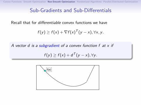
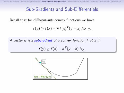
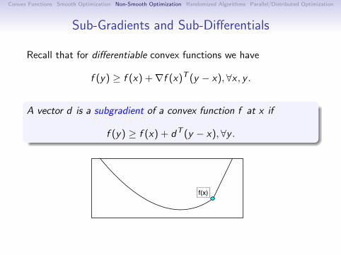
Sub-Gradients and Sub-Differentials
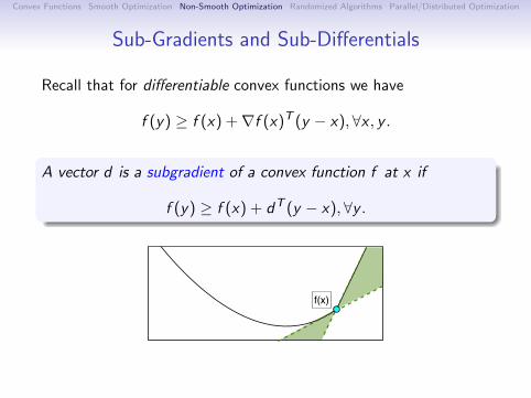
Recall that for differentiable convex functions we have
f (y) ≥ f (x) +∇f (x)T (y − x), ∀x , y .
A vector d is a subgradient of a convex function f at x if
f (y) ≥ f (x) + dT (y − x),∀y .

Convex Functions Smooth Optimization Non-Smooth Optimization Randomized Algorithms Parallel/Distributed Optimization
Sub-Gradients and Sub-Differentials
Recall that for differentiable convex functions we have
f (y) ≥ f (x) +∇f (x)T (y − x), ∀x , y .
A vector d is a subgradient of a convex function f at x if
f (y) ≥ f (x) + dT (y − x),∀y .
f(x)
f(x) + ∇f(x)T(y-x)
Convex Functions Smooth Optimization Non-Smooth Optimization Randomized Algorithms Parallel/Distributed Optimization
Sub-Gradients and Sub-Differentials
Recall that for differentiable convex functions we have
f (y) ≥ f (x) +∇f (x)T (y − x), ∀x , y .
A vector d is a subgradient of a convex function f at x if
f (y) ≥ f (x) + dT (y − x),∀y .
f(x)

Convex Functions Smooth Optimization Non-Smooth Optimization Randomized Algorithms Parallel/Distributed Optimization
Sub-Gradients and Sub-Differentials
Recall that for differentiable convex functions we have
f (y) ≥ f (x) +∇f (x)T (y − x), ∀x , y .
A vector d is a subgradient of a convex function f at x if
f (y) ≥ f (x) + dT (y − x),∀y .
f is differentiable at x iff ∇f (x) is the only subgradient.
At non-differentiable x , we have a set of subgradients.
Set of subgradients is the sub-differential ∂f (x).
Note that 0 ∈ ∂f (x) iff x is a global minimum.

Convex Functions Smooth Optimization Non-Smooth Optimization Randomized Algorithms Parallel/Distributed Optimization
Sub-Differential of Absolute Value and Max Functions
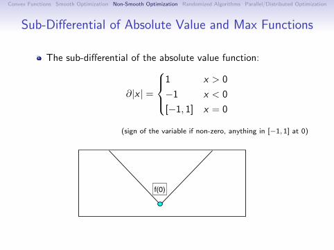
The sub-differential of the absolute value function:
∂|x | =
1 x > 0
−1 x < 0
[−1, 1] x = 0
(sign of the variable if non-zero, anything in [−1, 1] at 0)

Convex Functions Smooth Optimization Non-Smooth Optimization Randomized Algorithms Parallel/Distributed Optimization
Sub-Differential of Absolute Value and Max Functions
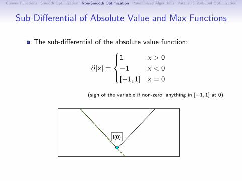
The sub-differential of the absolute value function:
∂|x | =
1 x > 0
−1 x < 0
[−1, 1] x = 0
(sign of the variable if non-zero, anything in [−1, 1] at 0)
f(x)

Convex Functions Smooth Optimization Non-Smooth Optimization Randomized Algorithms Parallel/Distributed Optimization
Sub-Differential of Absolute Value and Max Functions
The sub-differential of the absolute value function:
∂|x | =
1 x > 0
−1 x < 0
[−1, 1] x = 0
(sign of the variable if non-zero, anything in [−1, 1] at 0)
f(x)
Convex Functions Smooth Optimization Non-Smooth Optimization Randomized Algorithms Parallel/Distributed Optimization
Sub-Differential of Absolute Value and Max Functions
The sub-differential of the absolute value function:
∂|x | =
1 x > 0
−1 x < 0
[−1, 1] x = 0
(sign of the variable if non-zero, anything in [−1, 1] at 0)
f(0)
Convex Functions Smooth Optimization Non-Smooth Optimization Randomized Algorithms Parallel/Distributed Optimization
Sub-Differential of Absolute Value and Max Functions
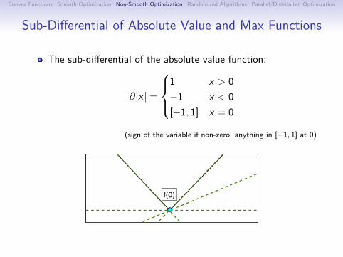
The sub-differential of the absolute value function:
∂|x | =
1 x > 0
−1 x < 0
[−1, 1] x = 0
(sign of the variable if non-zero, anything in [−1, 1] at 0)
f(0)

Convex Functions Smooth Optimization Non-Smooth Optimization Randomized Algorithms Parallel/Distributed Optimization
Sub-Differential of Absolute Value and Max Functions
The sub-differential of the absolute value function:
∂|x | =
1 x > 0
−1 x < 0
[−1, 1] x = 0
(sign of the variable if non-zero, anything in [−1, 1] at 0)
f(0)

Convex Functions Smooth Optimization Non-Smooth Optimization Randomized Algorithms Parallel/Distributed Optimization
Sub-Differential of Absolute Value and Max Functions
The sub-differential of the absolute value function:
∂|x | =
1 x > 0
−1 x < 0
[−1, 1] x = 0
(sign of the variable if non-zero, anything in [−1, 1] at 0)
The sub-differential of the maximum of differentiable fi :
∂maxf1(x), f2(x) =
∇f1(x) f1(x) > f2(x)
∇f2(x) f2(x) > f1(x)
θ∇f1(x) + (1− θ)∇f2(x) f1(x) = f2(x)
(any convex combination of the gradients of the argmax)

Convex Functions Smooth Optimization Non-Smooth Optimization Randomized Algorithms Parallel/Distributed Optimization
Sub-gradient methodThe sub-gradient method:
x+ = x − αd ,for some d ∈ ∂f (x).
The steepest descent step is given by argmind∈∂f (x)‖d‖.(often hard to compute, but easy for `1-regularization)
Otherwise, may increase the objective even for small α.But ‖x+ − x∗‖ ≤ ‖x − x∗‖ for small enough α.For convergence, we require α→ 0.Many variants average the iterations:
xk =k−1∑
i=0
wixi .
Many variants average the gradients (‘dual averaging’):
dk =k−1∑
i=0
widi .

Convex Functions Smooth Optimization Non-Smooth Optimization Randomized Algorithms Parallel/Distributed Optimization
Sub-gradient methodThe sub-gradient method:
x+ = x − αd ,for some d ∈ ∂f (x).The steepest descent step is given by argmind∈∂f (x)‖d‖.
(often hard to compute, but easy for `1-regularization)
Otherwise, may increase the objective even for small α.But ‖x+ − x∗‖ ≤ ‖x − x∗‖ for small enough α.For convergence, we require α→ 0.
Many variants average the iterations:
xk =k−1∑
i=0
wixi .
Many variants average the gradients (‘dual averaging’):
dk =k−1∑
i=0
widi .

Convex Functions Smooth Optimization Non-Smooth Optimization Randomized Algorithms Parallel/Distributed Optimization
Sub-gradient methodThe sub-gradient method:
x+ = x − αd ,for some d ∈ ∂f (x).The steepest descent step is given by argmind∈∂f (x)‖d‖.
(often hard to compute, but easy for `1-regularization)
Otherwise, may increase the objective even for small α.But ‖x+ − x∗‖ ≤ ‖x − x∗‖ for small enough α.For convergence, we require α→ 0.Many variants average the iterations:
xk =k−1∑
i=0
wixi .
Many variants average the gradients (‘dual averaging’):
dk =k−1∑
i=0
widi .

Convex Functions Smooth Optimization Non-Smooth Optimization Randomized Algorithms Parallel/Distributed Optimization
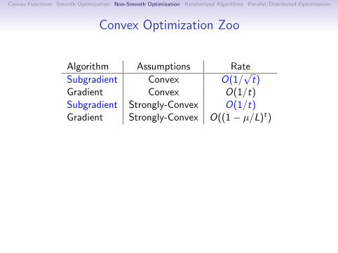
Convex Optimization Zoo
Algorithm Assumptions Rate
Subgradient Convex O(1/√t)
Gradient Convex O(1/t)
Subgradient Strongly-Convex O(1/t)Gradient Strongly-Convex O((1− µ/L)t)
Alternative is cutting-plane/bundle methods:
Minimze an approximation based on all subgradients dt.But have the same rates as the subgradient method.
(tend to be better in practice)
Bad news: Rates are optimal for black-box methods.
But, we often have more than a black-box.
Convex Functions Smooth Optimization Non-Smooth Optimization Randomized Algorithms Parallel/Distributed Optimization
Convex Optimization Zoo
Algorithm Assumptions Rate
Subgradient Convex O(1/√t)
Gradient Convex O(1/t)Subgradient Strongly-Convex O(1/t)Gradient Strongly-Convex O((1− µ/L)t)
Alternative is cutting-plane/bundle methods:
Minimze an approximation based on all subgradients dt.But have the same rates as the subgradient method.
(tend to be better in practice)
Bad news: Rates are optimal for black-box methods.
But, we often have more than a black-box.

Convex Functions Smooth Optimization Non-Smooth Optimization Randomized Algorithms Parallel/Distributed Optimization
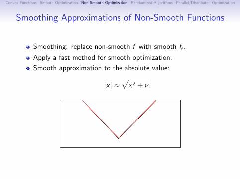
Smoothing Approximations of Non-Smooth Functions
Smoothing: replace non-smooth f with smooth fε.
Apply a fast method for smooth optimization.
Smooth approximation to the absolute value:
|x | ≈√x2 + ν.

Convex Functions Smooth Optimization Non-Smooth Optimization Randomized Algorithms Parallel/Distributed Optimization
Smoothing Approximations of Non-Smooth Functions
Smoothing: replace non-smooth f with smooth fε.
Apply a fast method for smooth optimization.
Smooth approximation to the absolute value:
|x | ≈√x2 + ν.
Smooth approximation to the max function:
maxa, b ≈ log(exp(a) + exp(b))
Smooth approximation to the hinge loss:
max0, x ≈
0 x ≥ 1
1− x2 t < x < 1
(1− t)2 + 2(1− t)(t − x) x ≤ t
Generic smoothing strategy: strongly-convex regularization ofconvex conjugate.[Nesterov, 2005]

Convex Functions Smooth Optimization Non-Smooth Optimization Randomized Algorithms Parallel/Distributed Optimization
Convex Optimization Zoo
Algorithm Assumptions Rate
Subgradient Convex O(1/√t)
Gradient Convex O(1/t)Nesterov Convex O(1/t2)
Gradient Smoothed to 1/ε, Convex O(1/√t)
Nesterov Smoothed to 1/ε, Convex O(1/t)
Smoothing is only faster if you use Nesterov’s method.
In practice, faster to slowly decrease smoothing level.
You can get the O(1/t) rate for minx maxfi (x) for fi convexand smooth using mirror-prox method.[Nemirovski, 2004]

Convex Functions Smooth Optimization Non-Smooth Optimization Randomized Algorithms Parallel/Distributed Optimization
Convex Optimization Zoo
Algorithm Assumptions Rate
Subgradient Convex O(1/√t)
Gradient Convex O(1/t)Nesterov Convex O(1/t2)Gradient Smoothed to 1/ε, Convex O(1/
√t)
Nesterov Smoothed to 1/ε, Convex O(1/t)
Smoothing is only faster if you use Nesterov’s method.
In practice, faster to slowly decrease smoothing level.
You can get the O(1/t) rate for minx maxfi (x) for fi convexand smooth using mirror-prox method.[Nemirovski, 2004]

Convex Functions Smooth Optimization Non-Smooth Optimization Randomized Algorithms Parallel/Distributed Optimization
Converting to Constrained Optimization
Re-write non-smooth problem as constrained problem.
The problemminx
f (x) + λ‖x‖1,
is equivalent to the problem
minx+≥0,x−≥0
f (x+ − x−) + λ∑
i
(x+i + x−i ),
or the problems
min−y≤x≤y
f (x) + λ∑
i
yi , min‖x‖1≤γ
f (x) + λγ
These are smooth objective with ‘simple’ constraints.
minx∈C
f (x).
Convex Functions Smooth Optimization Non-Smooth Optimization Randomized Algorithms Parallel/Distributed Optimization
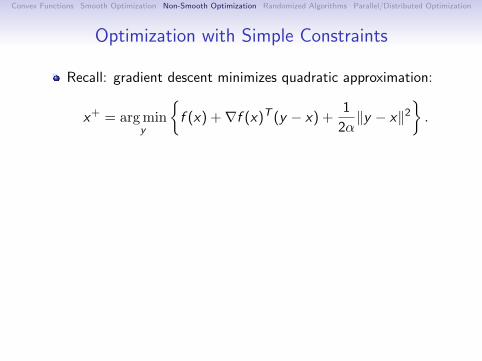
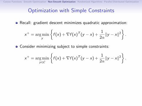
Optimization with Simple Constraints
Recall: gradient descent minimizes quadratic approximation:
x+ = argminy
f (x) +∇f (x)T (y − x) +
1
2α‖y − x‖2
.
Consider minimizing subject to simple constraints:
x+ = argminy∈C
f (x) +∇f (x)T (y − x) +
1
2α‖y − x‖2
.
Equivalent to projection of gradient descent:
xGD = x − α∇f (x),
x+ = argminy∈C
‖y − xGD‖
,
Convex Functions Smooth Optimization Non-Smooth Optimization Randomized Algorithms Parallel/Distributed Optimization
Optimization with Simple Constraints
Recall: gradient descent minimizes quadratic approximation:
x+ = argminy
f (x) +∇f (x)T (y − x) +
1
2α‖y − x‖2
.
Consider minimizing subject to simple constraints:
x+ = argminy∈C
f (x) +∇f (x)T (y − x) +
1
2α‖y − x‖2
.
Equivalent to projection of gradient descent:
xGD = x − α∇f (x),
x+ = argminy∈C
‖y − xGD‖
,

Convex Functions Smooth Optimization Non-Smooth Optimization Randomized Algorithms Parallel/Distributed Optimization
Optimization with Simple Constraints
Recall: gradient descent minimizes quadratic approximation:
x+ = argminy
f (x) +∇f (x)T (y − x) +
1
2α‖y − x‖2
.
Consider minimizing subject to simple constraints:
x+ = argminy∈C
f (x) +∇f (x)T (y − x) +
1
2α‖y − x‖2
.
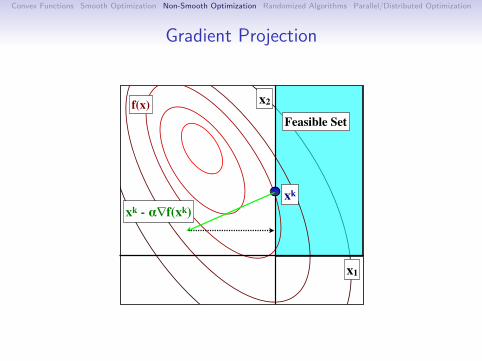
Equivalent to projection of gradient descent:
xGD = x − α∇f (x),
x+ = argminy∈C
‖y − xGD‖
,
Convex Functions Smooth Optimization Non-Smooth Optimization Randomized Algorithms Parallel/Distributed Optimization
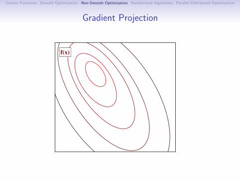
Gradient Projection
f(x)

Convex Functions Smooth Optimization Non-Smooth Optimization Randomized Algorithms Parallel/Distributed Optimization
Gradient Projection
f(x)
x1
x2

Convex Functions Smooth Optimization Non-Smooth Optimization Randomized Algorithms Parallel/Distributed Optimization
Gradient Projection
f(x)Feasible Set
x1
x2

Convex Functions Smooth Optimization Non-Smooth Optimization Randomized Algorithms Parallel/Distributed Optimization
Gradient Projection
f(x)Feasible Set
xk
x1
x2

Convex Functions Smooth Optimization Non-Smooth Optimization Randomized Algorithms Parallel/Distributed Optimization
Gradient Projection
f(x)Feasible Set
xk
x1
x2
xk - !!f(xk)
Convex Functions Smooth Optimization Non-Smooth Optimization Randomized Algorithms Parallel/Distributed Optimization
Gradient Projection
f(x)Feasible Set
xk
x1
x2
xk - !!f(xk)

Convex Functions Smooth Optimization Non-Smooth Optimization Randomized Algorithms Parallel/Distributed Optimization
Gradient Projection
f(x)Feasible Set
[xk - !!f(xk)]+
xk
x1
x2
xk - !!f(xk)

Convex Functions Smooth Optimization Non-Smooth Optimization Randomized Algorithms Parallel/Distributed Optimization
Projection Onto Simple Sets
Projections onto simple sets:
argminy≥0 ‖y − x‖ = maxx , 0
argminl≤y≤u ‖y − x‖ = maxl ,minx , uargminaT y=b ‖y − x‖ = x + (b − aT x)a/‖a‖2.
argminaT y≥b ‖y − x‖ =
x aT x ≥ b
x + (b − aT x)a/‖a‖2 aT x < b
argmin‖y‖≤τ ‖y − x‖ = τx/‖x‖.Linear-time algorithm for `1-norm ‖y‖1 ≤ τ .
Linear-time algorithm for probability simplex y ≥ 0,∑
y = 1.
Intersection of simple sets: Dykstra’s algorithm.
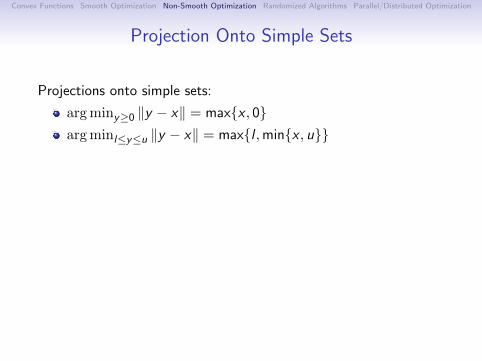
Convex Functions Smooth Optimization Non-Smooth Optimization Randomized Algorithms Parallel/Distributed Optimization
Projection Onto Simple Sets
Projections onto simple sets:
argminy≥0 ‖y − x‖ = maxx , 0argminl≤y≤u ‖y − x‖ = maxl ,minx , u
argminaT y=b ‖y − x‖ = x + (b − aT x)a/‖a‖2.
argminaT y≥b ‖y − x‖ =
x aT x ≥ b
x + (b − aT x)a/‖a‖2 aT x < b
argmin‖y‖≤τ ‖y − x‖ = τx/‖x‖.Linear-time algorithm for `1-norm ‖y‖1 ≤ τ .
Linear-time algorithm for probability simplex y ≥ 0,∑
y = 1.
Intersection of simple sets: Dykstra’s algorithm.

Convex Functions Smooth Optimization Non-Smooth Optimization Randomized Algorithms Parallel/Distributed Optimization
Projection Onto Simple Sets
Projections onto simple sets:
argminy≥0 ‖y − x‖ = maxx , 0argminl≤y≤u ‖y − x‖ = maxl ,minx , uargminaT y=b ‖y − x‖ = x + (b − aT x)a/‖a‖2.
argminaT y≥b ‖y − x‖ =
x aT x ≥ b
x + (b − aT x)a/‖a‖2 aT x < b
argmin‖y‖≤τ ‖y − x‖ = τx/‖x‖.Linear-time algorithm for `1-norm ‖y‖1 ≤ τ .
Linear-time algorithm for probability simplex y ≥ 0,∑
y = 1.
Intersection of simple sets: Dykstra’s algorithm.
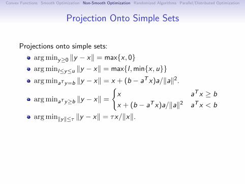
Convex Functions Smooth Optimization Non-Smooth Optimization Randomized Algorithms Parallel/Distributed Optimization
Projection Onto Simple Sets
Projections onto simple sets:
argminy≥0 ‖y − x‖ = maxx , 0argminl≤y≤u ‖y − x‖ = maxl ,minx , uargminaT y=b ‖y − x‖ = x + (b − aT x)a/‖a‖2.
argminaT y≥b ‖y − x‖ =
x aT x ≥ b
x + (b − aT x)a/‖a‖2 aT x < b
argmin‖y‖≤τ ‖y − x‖ = τx/‖x‖.
Linear-time algorithm for `1-norm ‖y‖1 ≤ τ .
Linear-time algorithm for probability simplex y ≥ 0,∑
y = 1.
Intersection of simple sets: Dykstra’s algorithm.
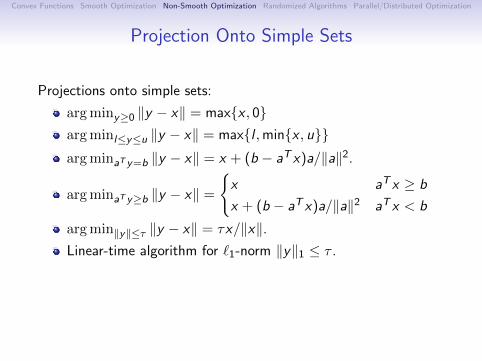
Convex Functions Smooth Optimization Non-Smooth Optimization Randomized Algorithms Parallel/Distributed Optimization
Projection Onto Simple Sets
Projections onto simple sets:
argminy≥0 ‖y − x‖ = maxx , 0argminl≤y≤u ‖y − x‖ = maxl ,minx , uargminaT y=b ‖y − x‖ = x + (b − aT x)a/‖a‖2.
argminaT y≥b ‖y − x‖ =
x aT x ≥ b
x + (b − aT x)a/‖a‖2 aT x < b
argmin‖y‖≤τ ‖y − x‖ = τx/‖x‖.Linear-time algorithm for `1-norm ‖y‖1 ≤ τ .
Linear-time algorithm for probability simplex y ≥ 0,∑
y = 1.
Intersection of simple sets: Dykstra’s algorithm.

Convex Functions Smooth Optimization Non-Smooth Optimization Randomized Algorithms Parallel/Distributed Optimization
Projection Onto Simple Sets
Projections onto simple sets:
argminy≥0 ‖y − x‖ = maxx , 0argminl≤y≤u ‖y − x‖ = maxl ,minx , uargminaT y=b ‖y − x‖ = x + (b − aT x)a/‖a‖2.
argminaT y≥b ‖y − x‖ =
x aT x ≥ b
x + (b − aT x)a/‖a‖2 aT x < b
argmin‖y‖≤τ ‖y − x‖ = τx/‖x‖.Linear-time algorithm for `1-norm ‖y‖1 ≤ τ .
Linear-time algorithm for probability simplex y ≥ 0,∑
y = 1.
Intersection of simple sets: Dykstra’s algorithm.

Convex Functions Smooth Optimization Non-Smooth Optimization Randomized Algorithms Parallel/Distributed Optimization
Convex Optimization Zoo
Algorithm Assumptions Rate
P(Subgradient) Convex O(1/√t)
P(Subgradient) Strongly O(1/t)P(Nesterov) Smoothed to 1/ε, Convex O(1/t)P(Gradient) Convex O(1/t)P(Nesterov) Convex O(1/t2)P(Gradient) Strongly O((1− µ/L)t)
P(Nesterov) Strongly O((1−√µ/L)t)
P(Newton) Strongly O(∏t
i=1 ρt), ρt → 0
Convergence rates are the same for projected versions!
Can do many of the same tricks (i.e. Armijo line-search,polynomial interpolation, Barzilai-Borwein, quasi-Newton).For Newton, you need to project under ‖ · ‖∇2f (x)
(expensive, but special tricks for the case of simplex or lower/upper bounds)
You don’t need to compute the projection exactly.
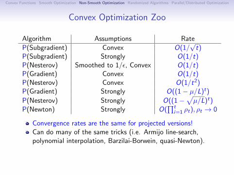
Convex Functions Smooth Optimization Non-Smooth Optimization Randomized Algorithms Parallel/Distributed Optimization
Convex Optimization Zoo
Algorithm Assumptions Rate
P(Subgradient) Convex O(1/√t)
P(Subgradient) Strongly O(1/t)P(Nesterov) Smoothed to 1/ε, Convex O(1/t)P(Gradient) Convex O(1/t)P(Nesterov) Convex O(1/t2)P(Gradient) Strongly O((1− µ/L)t)
P(Nesterov) Strongly O((1−√µ/L)t)
P(Newton) Strongly O(∏t
i=1 ρt), ρt → 0
Convergence rates are the same for projected versions!Can do many of the same tricks (i.e. Armijo line-search,polynomial interpolation, Barzilai-Borwein, quasi-Newton).
For Newton, you need to project under ‖ · ‖∇2f (x)
(expensive, but special tricks for the case of simplex or lower/upper bounds)
You don’t need to compute the projection exactly.

Convex Functions Smooth Optimization Non-Smooth Optimization Randomized Algorithms Parallel/Distributed Optimization
Convex Optimization Zoo
Algorithm Assumptions Rate
P(Subgradient) Convex O(1/√t)
P(Subgradient) Strongly O(1/t)P(Nesterov) Smoothed to 1/ε, Convex O(1/t)P(Gradient) Convex O(1/t)P(Nesterov) Convex O(1/t2)P(Gradient) Strongly O((1− µ/L)t)
P(Nesterov) Strongly O((1−√µ/L)t)
P(Newton) Strongly O(∏t
i=1 ρt), ρt → 0
Convergence rates are the same for projected versions!Can do many of the same tricks (i.e. Armijo line-search,polynomial interpolation, Barzilai-Borwein, quasi-Newton).For Newton, you need to project under ‖ · ‖∇2f (x)
(expensive, but special tricks for the case of simplex or lower/upper bounds)
You don’t need to compute the projection exactly.
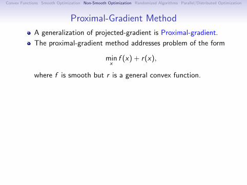
Convex Functions Smooth Optimization Non-Smooth Optimization Randomized Algorithms Parallel/Distributed Optimization
Proximal-Gradient Method
A generalization of projected-gradient is Proximal-gradient.
The proximal-gradient method addresses problem of the form
minx
f (x) + r(x),
where f is smooth but r is a general convex function.
Applies proximity operator of r to gradient descent on f :
xGD = x − α∇f (x),
x+ = argminy
1
2‖y − xGD‖2 + αr(y)
,
Equivalent to using the approximation
x+ = argminy
f (x) +∇f (x)T (y − x) +
1
2α‖y − x‖2+r(y)
.
Convergence rates are still the same as for minimizing f .
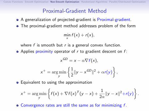
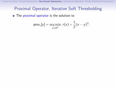
Convex Functions Smooth Optimization Non-Smooth Optimization Randomized Algorithms Parallel/Distributed Optimization
Proximal Operator, Iterative Soft Thresholding
The proximal operator is the solution to
proxr [y ] = argminx∈RP
r(x) +1
2‖x − y‖2.
For L1-regularization, we obtain iterative soft-thresholding:
x+ = softThreshαλ[x − α∇f (x)].
Example with λ = 1:Input Threshold Soft-Threshold
0.6715−1.20750.71721.63020.4889
0−1.2075
01.6302
0
0−0.2075
00.6302
0
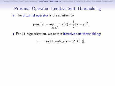
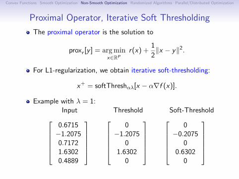

Convex Functions Smooth Optimization Non-Smooth Optimization Randomized Algorithms Parallel/Distributed Optimization
Special case of Projected-Gradient Methods
Projected-gradient methods are another special case:
r(x) =
0 if x ∈ C∞ if x /∈ C
,
givesx+ = projectC[x − α∇f (x)],
f(x)
x

Convex Functions Smooth Optimization Non-Smooth Optimization Randomized Algorithms Parallel/Distributed Optimization
Special case of Projected-Gradient Methods
Projected-gradient methods are another special case:
r(x) =
0 if x ∈ C∞ if x /∈ C
,
givesx+ = projectC[x − α∇f (x)],
f(x)
x

Convex Functions Smooth Optimization Non-Smooth Optimization Randomized Algorithms Parallel/Distributed Optimization
Special case of Projected-Gradient Methods
Projected-gradient methods are another special case:
r(x) =
0 if x ∈ C∞ if x /∈ C
,
givesx+ = projectC[x − α∇f (x)],
f(x)
x

Convex Functions Smooth Optimization Non-Smooth Optimization Randomized Algorithms Parallel/Distributed Optimization
Special case of Projected-Gradient Methods
Projected-gradient methods are another special case:
r(x) =
0 if x ∈ C∞ if x /∈ C
,
givesx+ = projectC[x − α∇f (x)],
Feasible Set
f(x)
x

Convex Functions Smooth Optimization Non-Smooth Optimization Randomized Algorithms Parallel/Distributed Optimization
Special case of Projected-Gradient Methods
Projected-gradient methods are another special case:
r(x) =
0 if x ∈ C∞ if x /∈ C
,
givesx+ = projectC[x − α∇f (x)],
Feasible Set
x - !f’(x)f(x)
x

Convex Functions Smooth Optimization Non-Smooth Optimization Randomized Algorithms Parallel/Distributed Optimization
Special case of Projected-Gradient Methods
Projected-gradient methods are another special case:
r(x) =
0 if x ∈ C∞ if x /∈ C
,
givesx+ = projectC[x − α∇f (x)],
Feasible Set
f(x)
x
x - !f’(x)
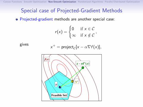
Convex Functions Smooth Optimization Non-Smooth Optimization Randomized Algorithms Parallel/Distributed Optimization
Special case of Projected-Gradient Methods
Projected-gradient methods are another special case:
r(x) =
0 if x ∈ C∞ if x /∈ C
,
givesx+ = projectC[x − α∇f (x)],
Feasible Set
x+
f(x)
x
x - !f’(x)
Convex Functions Smooth Optimization Non-Smooth Optimization Randomized Algorithms Parallel/Distributed Optimization
Exact Proximal-Gradient Methods
For what problems can we apply these methods?
We can efficiently compute the proximity operator for:1 L1-Regularization.2 Group `1-Regularization.3 Lower and upper bounds.4 Small number of linear constraint.5 Probability constraints.6 A few other simple regularizers/constraints.
Can solve these non-smooth/constrained problems as fast assmooth/unconstrained problems!
But for many problems we can not efficiently compute thisoperator.

Convex Functions Smooth Optimization Non-Smooth Optimization Randomized Algorithms Parallel/Distributed Optimization
Exact Proximal-Gradient Methods
For what problems can we apply these methods?
We can efficiently compute the proximity operator for:1 L1-Regularization.
2 Group `1-Regularization.3 Lower and upper bounds.4 Small number of linear constraint.5 Probability constraints.6 A few other simple regularizers/constraints.
Can solve these non-smooth/constrained problems as fast assmooth/unconstrained problems!
But for many problems we can not efficiently compute thisoperator.
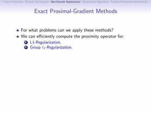
Convex Functions Smooth Optimization Non-Smooth Optimization Randomized Algorithms Parallel/Distributed Optimization
Exact Proximal-Gradient Methods
For what problems can we apply these methods?
We can efficiently compute the proximity operator for:1 L1-Regularization.2 Group `1-Regularization.
3 Lower and upper bounds.4 Small number of linear constraint.5 Probability constraints.6 A few other simple regularizers/constraints.
Can solve these non-smooth/constrained problems as fast assmooth/unconstrained problems!
But for many problems we can not efficiently compute thisoperator.

Convex Functions Smooth Optimization Non-Smooth Optimization Randomized Algorithms Parallel/Distributed Optimization
Exact Proximal-Gradient Methods
For what problems can we apply these methods?
We can efficiently compute the proximity operator for:1 L1-Regularization.2 Group `1-Regularization.3 Lower and upper bounds.
4 Small number of linear constraint.5 Probability constraints.6 A few other simple regularizers/constraints.
Can solve these non-smooth/constrained problems as fast assmooth/unconstrained problems!
But for many problems we can not efficiently compute thisoperator.
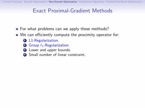
Convex Functions Smooth Optimization Non-Smooth Optimization Randomized Algorithms Parallel/Distributed Optimization
Exact Proximal-Gradient Methods
For what problems can we apply these methods?
We can efficiently compute the proximity operator for:1 L1-Regularization.2 Group `1-Regularization.3 Lower and upper bounds.4 Small number of linear constraint.
5 Probability constraints.6 A few other simple regularizers/constraints.
Can solve these non-smooth/constrained problems as fast assmooth/unconstrained problems!
But for many problems we can not efficiently compute thisoperator.

Convex Functions Smooth Optimization Non-Smooth Optimization Randomized Algorithms Parallel/Distributed Optimization
Exact Proximal-Gradient Methods
For what problems can we apply these methods?
We can efficiently compute the proximity operator for:1 L1-Regularization.2 Group `1-Regularization.3 Lower and upper bounds.4 Small number of linear constraint.5 Probability constraints.
6 A few other simple regularizers/constraints.
Can solve these non-smooth/constrained problems as fast assmooth/unconstrained problems!
But for many problems we can not efficiently compute thisoperator.

Convex Functions Smooth Optimization Non-Smooth Optimization Randomized Algorithms Parallel/Distributed Optimization
Exact Proximal-Gradient Methods
For what problems can we apply these methods?
We can efficiently compute the proximity operator for:1 L1-Regularization.2 Group `1-Regularization.3 Lower and upper bounds.4 Small number of linear constraint.5 Probability constraints.6 A few other simple regularizers/constraints.
Can solve these non-smooth/constrained problems as fast assmooth/unconstrained problems!
But for many problems we can not efficiently compute thisoperator.
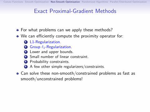
Convex Functions Smooth Optimization Non-Smooth Optimization Randomized Algorithms Parallel/Distributed Optimization
Exact Proximal-Gradient Methods
For what problems can we apply these methods?
We can efficiently compute the proximity operator for:1 L1-Regularization.2 Group `1-Regularization.3 Lower and upper bounds.4 Small number of linear constraint.5 Probability constraints.6 A few other simple regularizers/constraints.
Can solve these non-smooth/constrained problems as fast assmooth/unconstrained problems!
But for many problems we can not efficiently compute thisoperator.

Convex Functions Smooth Optimization Non-Smooth Optimization Randomized Algorithms Parallel/Distributed Optimization
Inexact Proximal-Gradient Methods
We can efficiently approximate the proximity operator for:
1 Structured sparsity.2 Penalties on the differences between variables.3 Regularizers and constraints on the singular values of matrices.4 Sums of simple functions.
Many recent works use inexact proximal-gradient methods:Cai et al. [2010], Liu & Ye [2010], Barbero & Sra [2011], Fadili & Peyre [2011],
Ma et al. [2011]
Do inexact methods have the same rates?
Yes, if the errors are appropriately controlled. [Schmidt et al.,
2011]

Convex Functions Smooth Optimization Non-Smooth Optimization Randomized Algorithms Parallel/Distributed Optimization
Inexact Proximal-Gradient Methods
We can efficiently approximate the proximity operator for:1 Structured sparsity.
2 Penalties on the differences between variables.3 Regularizers and constraints on the singular values of matrices.4 Sums of simple functions.
Many recent works use inexact proximal-gradient methods:Cai et al. [2010], Liu & Ye [2010], Barbero & Sra [2011], Fadili & Peyre [2011],
Ma et al. [2011]
Do inexact methods have the same rates?
Yes, if the errors are appropriately controlled. [Schmidt et al.,
2011]

Convex Functions Smooth Optimization Non-Smooth Optimization Randomized Algorithms Parallel/Distributed Optimization
Inexact Proximal-Gradient Methods
We can efficiently approximate the proximity operator for:1 Structured sparsity.2 Penalties on the differences between variables.
3 Regularizers and constraints on the singular values of matrices.4 Sums of simple functions.
Many recent works use inexact proximal-gradient methods:Cai et al. [2010], Liu & Ye [2010], Barbero & Sra [2011], Fadili & Peyre [2011],
Ma et al. [2011]
Do inexact methods have the same rates?
Yes, if the errors are appropriately controlled. [Schmidt et al.,
2011]
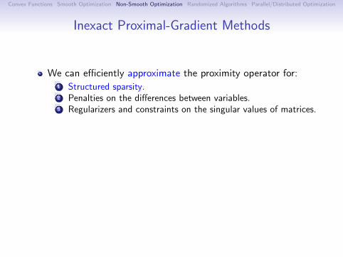
Convex Functions Smooth Optimization Non-Smooth Optimization Randomized Algorithms Parallel/Distributed Optimization
Inexact Proximal-Gradient Methods
We can efficiently approximate the proximity operator for:1 Structured sparsity.2 Penalties on the differences between variables.3 Regularizers and constraints on the singular values of matrices.
4 Sums of simple functions.
Many recent works use inexact proximal-gradient methods:Cai et al. [2010], Liu & Ye [2010], Barbero & Sra [2011], Fadili & Peyre [2011],
Ma et al. [2011]
Do inexact methods have the same rates?
Yes, if the errors are appropriately controlled. [Schmidt et al.,
2011]
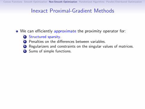
Convex Functions Smooth Optimization Non-Smooth Optimization Randomized Algorithms Parallel/Distributed Optimization
Inexact Proximal-Gradient Methods
We can efficiently approximate the proximity operator for:1 Structured sparsity.2 Penalties on the differences between variables.3 Regularizers and constraints on the singular values of matrices.4 Sums of simple functions.
Many recent works use inexact proximal-gradient methods:Cai et al. [2010], Liu & Ye [2010], Barbero & Sra [2011], Fadili & Peyre [2011],
Ma et al. [2011]
Do inexact methods have the same rates?
Yes, if the errors are appropriately controlled. [Schmidt et al.,
2011]
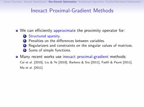
Convex Functions Smooth Optimization Non-Smooth Optimization Randomized Algorithms Parallel/Distributed Optimization
Inexact Proximal-Gradient Methods
We can efficiently approximate the proximity operator for:1 Structured sparsity.2 Penalties on the differences between variables.3 Regularizers and constraints on the singular values of matrices.4 Sums of simple functions.
Many recent works use inexact proximal-gradient methods:Cai et al. [2010], Liu & Ye [2010], Barbero & Sra [2011], Fadili & Peyre [2011],
Ma et al. [2011]
Do inexact methods have the same rates?
Yes, if the errors are appropriately controlled. [Schmidt et al.,
2011]

Convex Functions Smooth Optimization Non-Smooth Optimization Randomized Algorithms Parallel/Distributed Optimization
Convergence Rate of Inexact Proximal-Gradient
Proposition [Schmidt et al., 2011] If the sequences of gradienterrors ||et || and proximal errors √εt are in O((1− µ/L)t),then the inexact proximal-gradient method has an error ofO((1− µ/L)t).
Classic result as a special case (constants are good).
The rates degrades gracefully if the errors are larger.
Similar analyses in convex case.
Huge improvement in practice over black-box methods.
Also exist accelerated and spectral proximal-gradient methods.
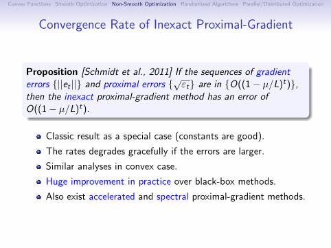

Convex Functions Smooth Optimization Non-Smooth Optimization Randomized Algorithms Parallel/Distributed Optimization
Discussion of Proximal-Gradient
Theoretical justification for what works in practice.
Significantly extends class of tractable problems.
Many applications with inexact proximal operators:
Genomic expression, model predictive control, neuroimaging,satellite image fusion, simulating flow fields.
But, it assumes computing ∇f (x) and proxh[x ] have similarcost.
Often ∇f (x) is much more expensive:
We may have a large dataset.Data-fitting term might be complex.
Particularly true for structured output prediction:
Text, biological sequences, speech, images, matchings, graphs.
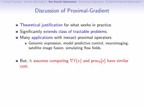
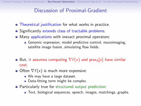

Convex Functions Smooth Optimization Non-Smooth Optimization Randomized Algorithms Parallel/Distributed Optimization
Costly Data-Fitting Term, Simple Regularizer
Consider fitting a conditional random field with`1-regularization:
minx∈RP
1
N
N∑
i=1
fi (x) + r(x)
costly smooth + simple
Different than classic optimization (like linear programming).(cheap smooth plus complex non-smooth)
Inspiration from the smooth case:
For smooth high-dimensional problems, L-BFGS quasi-Newtonalgorithm outperforms accelerated/spectral gradient methods.
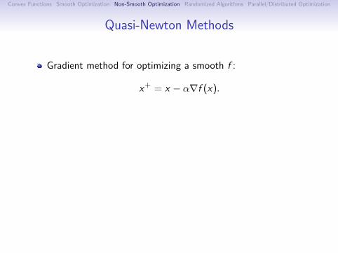
Convex Functions Smooth Optimization Non-Smooth Optimization Randomized Algorithms Parallel/Distributed Optimization
Quasi-Newton Methods
Gradient method for optimizing a smooth f :
x+ = x − α∇f (x).
Newton-like methods alternatively use:
x+ = x − αH−1∇f (x).
H approximates the second-derivative matrix.
L-BFGS is a particular strategy to choose the H values:
Based on gradient differences.Linear storage and linear time.
http://www.di.ens.fr/~mschmidt/Software/minFunc.html

Convex Functions Smooth Optimization Non-Smooth Optimization Randomized Algorithms Parallel/Distributed Optimization
Gradient Method and Newton’s Method
f(x)

Convex Functions Smooth Optimization Non-Smooth Optimization Randomized Algorithms Parallel/Distributed Optimization
Gradient Method and Newton’s Method
f(x)
x

Convex Functions Smooth Optimization Non-Smooth Optimization Randomized Algorithms Parallel/Distributed Optimization
Gradient Method and Newton’s Method
f(x)
x - !f’(x)
x

Convex Functions Smooth Optimization Non-Smooth Optimization Randomized Algorithms Parallel/Distributed Optimization
Gradient Method and Newton’s Method
Q(x)f(x)
x
x - !f’(x)
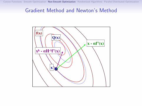
Convex Functions Smooth Optimization Non-Smooth Optimization Randomized Algorithms Parallel/Distributed Optimization
Gradient Method and Newton’s Method
f(x)
xk - !H-1f’(x)
x
x - !f’(x)Q(x)

Convex Functions Smooth Optimization Non-Smooth Optimization Randomized Algorithms Parallel/Distributed Optimization
Naive Proximal Quasi-Newton Method
Proximal-gradient method:
x+ = proxαr [x − α∇f (x)].
Can we just plug in the Newton-like step?
x+ = proxαr [x − αH−1∇f (x)].
NO!
f(x)

Convex Functions Smooth Optimization Non-Smooth Optimization Randomized Algorithms Parallel/Distributed Optimization
Naive Proximal Quasi-Newton Method
Proximal-gradient method:
x+ = proxαr [x − α∇f (x)].
Can we just plug in the Newton-like step?
x+ = proxαr [x − αH−1∇f (x)].
NO!
f(x)

Convex Functions Smooth Optimization Non-Smooth Optimization Randomized Algorithms Parallel/Distributed Optimization
Naive Proximal Quasi-Newton Method
Proximal-gradient method:
x+ = proxαr [x − α∇f (x)].
Can we just plug in the Newton-like step?
x+ = proxαr [x − αH−1∇f (x)].
NO!
f(x)

Convex Functions Smooth Optimization Non-Smooth Optimization Randomized Algorithms Parallel/Distributed Optimization
Naive Proximal Quasi-Newton Method
Proximal-gradient method:
x+ = proxαr [x − α∇f (x)].
Can we just plug in the Newton-like step?
x+ = proxαr [x − αH−1∇f (x)].
NO! f(x)

Convex Functions Smooth Optimization Non-Smooth Optimization Randomized Algorithms Parallel/Distributed Optimization
Naive Proximal Quasi-Newton Method
Proximal-gradient method:
x+ = proxαr [x − α∇f (x)].
Can we just plug in the Newton-like step?
x+ = proxαr [x − αH−1∇f (x)].
NO! f(x)
x1
x2
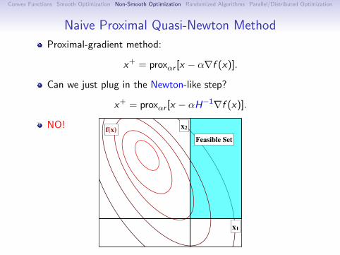
Convex Functions Smooth Optimization Non-Smooth Optimization Randomized Algorithms Parallel/Distributed Optimization
Naive Proximal Quasi-Newton Method
Proximal-gradient method:
x+ = proxαr [x − α∇f (x)].
Can we just plug in the Newton-like step?
x+ = proxαr [x − αH−1∇f (x)].
NO! f(x)Feasible Set
x
x1
x2
x - !f’(x)
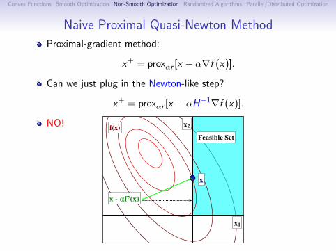
Convex Functions Smooth Optimization Non-Smooth Optimization Randomized Algorithms Parallel/Distributed Optimization
Naive Proximal Quasi-Newton Method
Proximal-gradient method:
x+ = proxαr [x − α∇f (x)].
Can we just plug in the Newton-like step?
x+ = proxαr [x − αH−1∇f (x)].
NO! f(x)Feasible Set
x+
x1
x2
x
x - !f’(x)

Convex Functions Smooth Optimization Non-Smooth Optimization Randomized Algorithms Parallel/Distributed Optimization
Naive Proximal Quasi-Newton Method
Proximal-gradient method:
x+ = proxαr [x − α∇f (x)].
Can we just plug in the Newton-like step?
x+ = proxαr [x − αH−1∇f (x)].
NO! f(x)Feasible Set
x1
x2Q(x)
x
x - !f’(x) x+

Convex Functions Smooth Optimization Non-Smooth Optimization Randomized Algorithms Parallel/Distributed Optimization
Naive Proximal Quasi-Newton Method
Proximal-gradient method:
x+ = proxαr [x − α∇f (x)].
Can we just plug in the Newton-like step?
x+ = proxαr [x − αH−1∇f (x)].
NO! f(x)Feasible Set
x1
x2
xk - !H-1f’(x)x
x - !f’(x) x+
Q(x)
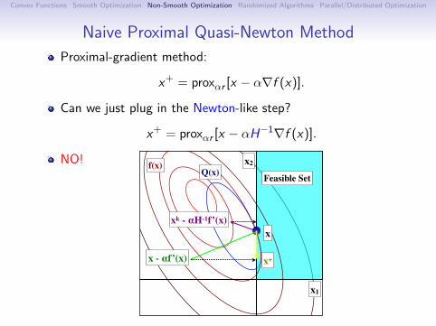
Convex Functions Smooth Optimization Non-Smooth Optimization Randomized Algorithms Parallel/Distributed Optimization
Naive Proximal Quasi-Newton Method
Proximal-gradient method:
x+ = proxαr [x − α∇f (x)].
Can we just plug in the Newton-like step?
x+ = proxαr [x − αH−1∇f (x)].
NO! f(x)Feasible Set
x1
x2
x
x - !f’(x) x+
Q(x)
xk - !H-1f’(x)

Convex Functions Smooth Optimization Non-Smooth Optimization Randomized Algorithms Parallel/Distributed Optimization
Naive Proximal Quasi-Newton Method
Proximal-gradient method:
x+ = proxαr [x − α∇f (x)].
Can we just plug in the Newton-like step?
x+ = proxαr [x − αH−1∇f (x)].
NO! f(x)Feasible Set
x1
x2
x+
x
x - !f’(x) x+
Q(x)
xk - !H-1f’(x)

Convex Functions Smooth Optimization Non-Smooth Optimization Randomized Algorithms Parallel/Distributed Optimization
Two-Metric (Sub)Gradient Projection
In some cases, we can modify H to make this work:
Bound constraints.Probability constraints.L1-regularization.
Two-metric (sub)gradient projection.[Gafni & Bertskeas, 1984, Schmidt, 2010].
Key idea: make H diagonal with respect to coordinates nearnon-differentiability.

Convex Functions Smooth Optimization Non-Smooth Optimization Randomized Algorithms Parallel/Distributed Optimization
Comparing to accelerated/spectral/diagonal gradientComparing to methods that do not use L-BFGS (sido data):
200 400 600 800 1000 1200 1400 1600 1800 2000
10−4
10−2
100
102
Function Evaluations
Ob
jec
tiv
e V
alu
e m
inu
s O
ptim
al
PSSgb
BBSG
BBST
OPG
SPG
DSST
http://www.di.ens.fr/~mschmidt/Software/L1General.html
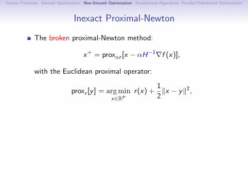
Convex Functions Smooth Optimization Non-Smooth Optimization Randomized Algorithms Parallel/Distributed Optimization
Inexact Proximal-Newton
The broken proximal-Newton method:
x+ = proxαr [x − αH−1∇f (x)],
with the Euclidean proximal operator:
proxr [y ] = argminx∈RP
r(x) +1
2‖x − y‖2,
where ‖x‖2H = xTHx .
Non-smooth Newton-like method
Same convergence properties as smooth case.
But, the prox is expensive even with a simple regularizer.
Solution: use a cheap approximate solution.(e.g., spectral proximal-gradient)

Convex Functions Smooth Optimization Non-Smooth Optimization Randomized Algorithms Parallel/Distributed Optimization
Inexact Proximal-Newton
The fixed proximal-Newton method:
x+ = proxαr [x − αH−1∇f (x)]H ,
with the non-Euclidean proximal operator:
proxr [y ]H = argminx∈RP
r(x) +1
2‖x − y‖2
H ,
where ‖x‖2H = xTHx .
Non-smooth Newton-like method
Same convergence properties as smooth case.
But, the prox is expensive even with a simple regularizer.
Solution: use a cheap approximate solution.(e.g., spectral proximal-gradient)
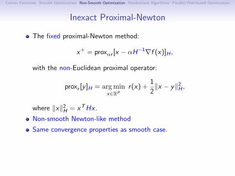
Convex Functions Smooth Optimization Non-Smooth Optimization Randomized Algorithms Parallel/Distributed Optimization
Inexact Proximal-Newton
The fixed proximal-Newton method:
x+ = proxαr [x − αH−1∇f (x)]H ,
with the non-Euclidean proximal operator:
proxr [y ]H = argminx∈RP
r(x) +1
2‖x − y‖2
H ,
where ‖x‖2H = xTHx .
Non-smooth Newton-like method
Same convergence properties as smooth case.
But, the prox is expensive even with a simple regularizer.
Solution: use a cheap approximate solution.(e.g., spectral proximal-gradient)

Convex Functions Smooth Optimization Non-Smooth Optimization Randomized Algorithms Parallel/Distributed Optimization
Inexact Projected Newton
f(x)
x

Convex Functions Smooth Optimization Non-Smooth Optimization Randomized Algorithms Parallel/Distributed Optimization
Inexact Projected Newton
Feasible Set
f(x)
x

Convex Functions Smooth Optimization Non-Smooth Optimization Randomized Algorithms Parallel/Distributed Optimization
Inexact Projected Newton
Feasible Set
x - !f’(x)f(x)
x

Convex Functions Smooth Optimization Non-Smooth Optimization Randomized Algorithms Parallel/Distributed Optimization
Inexact Projected Newton
Feasible Set
f(x)
x
x - !f’(x)

Convex Functions Smooth Optimization Non-Smooth Optimization Randomized Algorithms Parallel/Distributed Optimization
Inexact Projected Newton
Feasible Set
x+
f(x)
x
x - !f’(x)

Convex Functions Smooth Optimization Non-Smooth Optimization Randomized Algorithms Parallel/Distributed Optimization
Inexact Projected Newton
Feasible Set
f(x)
x

Convex Functions Smooth Optimization Non-Smooth Optimization Randomized Algorithms Parallel/Distributed Optimization
Inexact Projected Newton
Feasible Set
f(x)Q(y)
y0=x

Convex Functions Smooth Optimization Non-Smooth Optimization Randomized Algorithms Parallel/Distributed Optimization
Inexact Projected Newton
Feasible Set
f(x)Q(y)
y1
y0 - !Q’(y0)
y0=x

Convex Functions Smooth Optimization Non-Smooth Optimization Randomized Algorithms Parallel/Distributed Optimization
Inexact Projected Newton
Feasible Set
f(x)Q(y)
y1
y0=x
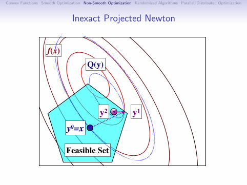
Convex Functions Smooth Optimization Non-Smooth Optimization Randomized Algorithms Parallel/Distributed Optimization
Inexact Projected Newton
Feasible Set
f(x)Q(y)
y1
y0=x
y2

Convex Functions Smooth Optimization Non-Smooth Optimization Randomized Algorithms Parallel/Distributed Optimization
Inexact Projected Newton
Feasible Set
f(x)Q(y)
y1
y0=x
y2
y3
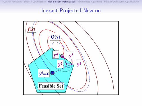
Convex Functions Smooth Optimization Non-Smooth Optimization Randomized Algorithms Parallel/Distributed Optimization
Inexact Projected Newton
Feasible Set
f(x)Q(y)
y0=x
y4
y1y2
y3

Convex Functions Smooth Optimization Non-Smooth Optimization Randomized Algorithms Parallel/Distributed Optimization
Inexact Projected Newton
Feasible Set
f(x)Q(y)
y0=x
x+=yt
Convex Functions Smooth Optimization Non-Smooth Optimization Randomized Algorithms Parallel/Distributed Optimization
Projected Quasi-Newton (PQN) Algorithm
A proximal quasi-Newton (PQN) algorithm:[Schmidt et al., 2009, Schmidt, 2010]
Outer: evaluate f (x) and ∇f (x), use L-BFGS to update H.Inner: spectral proximal-gradient to approximate proximaloperator:
Requires multiplication by H (linear-time for L-BFGS).Requires proximal operator of r (cheap for simple constraints).
For small α, one iteration is sufficient to give descent.
Cheap inner iterations lead to fewer expensive outer iterations.
“Optimizing costly functions with simple constraints”.
“Optimizing costly functions with simple regularizers”.

Convex Functions Smooth Optimization Non-Smooth Optimization Randomized Algorithms Parallel/Distributed Optimization
Projected Quasi-Newton (PQN) Algorithm
A proximal quasi-Newton (PQN) algorithm:[Schmidt et al., 2009, Schmidt, 2010]
Outer: evaluate f (x) and ∇f (x), use L-BFGS to update H.
Inner: spectral proximal-gradient to approximate proximaloperator:
Requires multiplication by H (linear-time for L-BFGS).Requires proximal operator of r (cheap for simple constraints).
For small α, one iteration is sufficient to give descent.
Cheap inner iterations lead to fewer expensive outer iterations.
“Optimizing costly functions with simple constraints”.
“Optimizing costly functions with simple regularizers”.

Convex Functions Smooth Optimization Non-Smooth Optimization Randomized Algorithms Parallel/Distributed Optimization
Projected Quasi-Newton (PQN) Algorithm
A proximal quasi-Newton (PQN) algorithm:[Schmidt et al., 2009, Schmidt, 2010]
Outer: evaluate f (x) and ∇f (x), use L-BFGS to update H.Inner: spectral proximal-gradient to approximate proximaloperator:
Requires multiplication by H (linear-time for L-BFGS).Requires proximal operator of r (cheap for simple constraints).
For small α, one iteration is sufficient to give descent.
Cheap inner iterations lead to fewer expensive outer iterations.
“Optimizing costly functions with simple constraints”.
“Optimizing costly functions with simple regularizers”.

Convex Functions Smooth Optimization Non-Smooth Optimization Randomized Algorithms Parallel/Distributed Optimization
Projected Quasi-Newton (PQN) Algorithm
A proximal quasi-Newton (PQN) algorithm:[Schmidt et al., 2009, Schmidt, 2010]
Outer: evaluate f (x) and ∇f (x), use L-BFGS to update H.Inner: spectral proximal-gradient to approximate proximaloperator:
Requires multiplication by H (linear-time for L-BFGS).Requires proximal operator of r (cheap for simple constraints).
For small α, one iteration is sufficient to give descent.
Cheap inner iterations lead to fewer expensive outer iterations.
“Optimizing costly functions with simple constraints”.
“Optimizing costly functions with simple regularizers”.
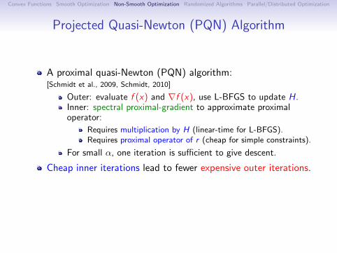
Convex Functions Smooth Optimization Non-Smooth Optimization Randomized Algorithms Parallel/Distributed Optimization
Projected Quasi-Newton (PQN) Algorithm
A proximal quasi-Newton (PQN) algorithm:[Schmidt et al., 2009, Schmidt, 2010]
Outer: evaluate f (x) and ∇f (x), use L-BFGS to update H.Inner: spectral proximal-gradient to approximate proximaloperator:
Requires multiplication by H (linear-time for L-BFGS).Requires proximal operator of r (cheap for simple constraints).
For small α, one iteration is sufficient to give descent.
Cheap inner iterations lead to fewer expensive outer iterations.
“Optimizing costly functions with simple constraints”.
“Optimizing costly functions with simple regularizers”.
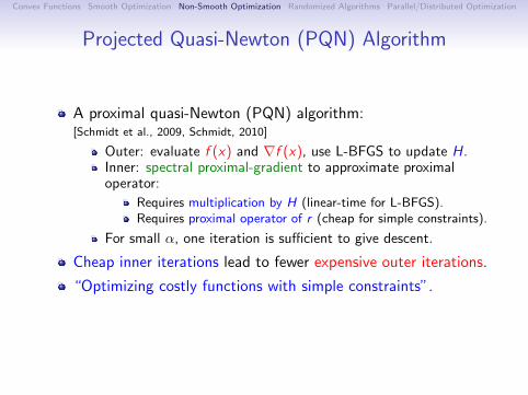
Convex Functions Smooth Optimization Non-Smooth Optimization Randomized Algorithms Parallel/Distributed Optimization
Projected Quasi-Newton (PQN) Algorithm
A proximal quasi-Newton (PQN) algorithm:[Schmidt et al., 2009, Schmidt, 2010]
Outer: evaluate f (x) and ∇f (x), use L-BFGS to update H.Inner: spectral proximal-gradient to approximate proximaloperator:
Requires multiplication by H (linear-time for L-BFGS).Requires proximal operator of r (cheap for simple constraints).
For small α, one iteration is sufficient to give descent.
Cheap inner iterations lead to fewer expensive outer iterations.
“Optimizing costly functions with simple constraints”.
“Optimizing costly functions with simple regularizers”.

Convex Functions Smooth Optimization Non-Smooth Optimization Randomized Algorithms Parallel/Distributed Optimization
Graphical Model Structure Learning with Groups
Comparing PQN to first-order methods on a graphical modelstructure learning problem. [Gasch et al., 2000, Duchi et al., 2008].
200 400 600 800 1000
−400
−380
−360
−340
−320
−300
−280
Function Evaluations
Ob
jec
tive
Va
lue
PQN
PG
SPG

Convex Functions Smooth Optimization Non-Smooth Optimization Randomized Algorithms Parallel/Distributed Optimization
Alternating Direction Method of Multipliers
Alernating direction method of multipliers (ADMM) solves:
minAx+By=c
f (x) + r(y).
Alternate between prox-like operators with respect to f and r .
Can introduce constraints to convert to this form:
minx
f (Ax) + r(x) ⇔ minx=Ay
f (x) + r(y),
minx
f (x) + r(Bx) ⇔ miny=Bx
f (x) + r(y).
If prox can not be computed exactly: Linearized ADMM.
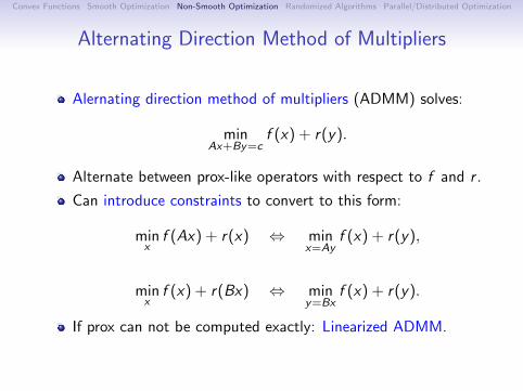

Convex Functions Smooth Optimization Non-Smooth Optimization Randomized Algorithms Parallel/Distributed Optimization
Dual Methods
Stronly-convex problems have smooth duals.
Solve the dual instead of the primal.
SVM non-smooth strongly-convex primal:
minx
CN∑
i=1
max0, 1− biaTi x+
1
2‖x‖2.
SVM smooth dual:
min0≤α≤C
1
2αTAATα−
N∑
i=1
αi
Smooth bound constrained problem:
Two-metric projection (efficient Newton-liked method).Randomized coordinate descent (next section).

Convex Functions Smooth Optimization Non-Smooth Optimization Randomized Algorithms Parallel/Distributed Optimization
Discussion
State of the art methods consider several other issues:
Shrinking: Identify variables likely to stay zero.[El Ghaoui et al., 2010].Continuation: Start with a large λ and slowly decrease it.[Xiao and Zhang, 2012]
Frank-Wolfe: Using linear approximations to obtainefficient/sparse updates.

Convex Functions Smooth Optimization Non-Smooth Optimization Randomized Algorithms Parallel/Distributed Optimization
Frank-Wolfe Method
In some cases the projected gradient step
x+ = argminy∈C
f (x) +∇f (x)T (y − x) +
1
2α‖y − x‖2
,
may be hard to compute (e.g., dual of max-margin Markovnetworks).
Frank-Wolfe method simply uses:
x+ = argminy∈C
f (x) +∇f (x)T (y − x)
,
requires compact C, takes convex combination of x and x+.
Iterate can be written as convex combination of vertices of C.
O(1/t) rate for smooth convex objectives, some linearconvergence results for smooth and strongly-convex.[Jaggi, 2013]

Convex Functions Smooth Optimization Non-Smooth Optimization Randomized Algorithms Parallel/Distributed Optimization
Outline
1 Convex Functions
2 Smooth Optimization
3 Non-Smooth Optimization
4 Randomized Algorithms
5 Parallel/Distributed Optimization
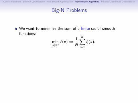
Convex Functions Smooth Optimization Non-Smooth Optimization Randomized Algorithms Parallel/Distributed Optimization
Big-N Problems
We want to minimize the sum of a finite set of smoothfunctions:
minx∈RP
f (x) :=1
N
N∑
i=1
fi (x).
We are interested in cases where N is very large.
Simple example is least-squares,
fi (x) := (aTi x − bi )2.
Other examples:
logistic regression, Huber regression, smooth SVMs, CRFs, etc.
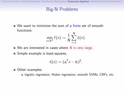

Convex Functions Smooth Optimization Non-Smooth Optimization Randomized Algorithms Parallel/Distributed Optimization
Stochastic vs. Deterministic Gradient MethodsWe consider minimizing f (x) = 1
N
∑Ni=1 fi (x).
Deterministic gradient method [Cauchy, 1847]:
xt+1 = xt − αt∇f (xt) = xt −αt
N
N∑
i=1
∇fi (xt).Iteration cost is linear in N.Quasi-Newton methods still require O(N).Convergence with constant αt or line-search.
Stochastic gradient method [Robbins & Monro, 1951]:Random selection of i(t) from 1, 2, . . . ,N.
xt+1 = xt − αt f′i(t)(xt).
Gives unbiased estimate of true gradient,
E[f ′(it)(x)] =1
N
N∑
i=1
∇fi (x) = ∇f (x).
Iteration cost is independent of N.As in subgradient method, we require αt → 0.Classical choice is αt = O(1/t).

Convex Functions Smooth Optimization Non-Smooth Optimization Randomized Algorithms Parallel/Distributed Optimization
Stochastic vs. Deterministic Gradient MethodsWe consider minimizing f (x) = 1
N
∑Ni=1 fi (x).
Deterministic gradient method [Cauchy, 1847]:
xt+1 = xt − αt∇f (xt) = xt −αt
N
N∑
i=1
∇fi (xt).Iteration cost is linear in N.Quasi-Newton methods still require O(N).Convergence with constant αt or line-search.
Stochastic gradient method [Robbins & Monro, 1951]:Random selection of i(t) from 1, 2, . . . ,N.
xt+1 = xt − αt f′i(t)(xt).
Gives unbiased estimate of true gradient,
E[f ′(it)(x)] =1
N
N∑
i=1
∇fi (x) = ∇f (x).
Iteration cost is independent of N.
As in subgradient method, we require αt → 0.Classical choice is αt = O(1/t).

Convex Functions Smooth Optimization Non-Smooth Optimization Randomized Algorithms Parallel/Distributed Optimization
Stochastic vs. Deterministic Gradient MethodsWe consider minimizing f (x) = 1
N
∑Ni=1 fi (x).
Deterministic gradient method [Cauchy, 1847]:
xt+1 = xt − αt∇f (xt) = xt −αt
N
N∑
i=1
∇fi (xt).Iteration cost is linear in N.Quasi-Newton methods still require O(N).Convergence with constant αt or line-search.
Stochastic gradient method [Robbins & Monro, 1951]:Random selection of i(t) from 1, 2, . . . ,N.
xt+1 = xt − αt f′i(t)(xt).
Gives unbiased estimate of true gradient,
E[f ′(it)(x)] =1
N
N∑
i=1
∇fi (x) = ∇f (x).
Iteration cost is independent of N.As in subgradient method, we require αt → 0.Classical choice is αt = O(1/t).

Convex Functions Smooth Optimization Non-Smooth Optimization Randomized Algorithms Parallel/Distributed Optimization
Stochastic vs. Deterministic Gradient Methods
We consider minimizing g(x) = 1N
∑ni=1 fi (x).
Deterministic gradient method [Cauchy, 1847]:
Stochastic vs. deterministic methods
• Minimizing g(!) =1
n
n!
i=1
fi(!) with fi(!) = ""yi, !
!!(xi)#
+ µ"(!)
• Batch gradient descent: !t = !t"1!#tg#(!t"1) = !t"1!
#t
n
n!
i=1
f #i(!t"1)
• Stochastic gradient descent: !t = !t"1 ! #tf#i(t)(!t"1)
Stochastic gradient method [Robbins & Monro, 1951]:
Stochastic vs. deterministic methods
• Minimizing g(!) =1
n
n!
i=1
fi(!) with fi(!) = ""yi, !
!!(xi)#
+ µ"(!)
• Batch gradient descent: !t = !t"1!#tg#(!t"1) = !t"1!
#t
n
n!
i=1
f #i(!t"1)
• Stochastic gradient descent: !t = !t"1 ! #tf#i(t)(!t"1)

Convex Functions Smooth Optimization Non-Smooth Optimization Randomized Algorithms Parallel/Distributed Optimization
Convex Optimization Zoo
Stochastic iterations are N times faster, but how many iterations?
Algorithm Assumptions Exact Stochastic
Subgradient Convex O(1/√t) O(1/
√t)
Subgradient Strongly O(1/t) O(1/t)
Good news for non-smooth problems:
stochastic is as fast as deterministic
We can solve non-smooth problems N times faster!
Bad news for smooth problems:
smoothness does not help stochastic methods.
Algorithm Assumptions Exact Stochastic
Gradient Convex O(1/t) O(1/√t)
Gradient Strongly O((1− µ/L)t) O(1/t)
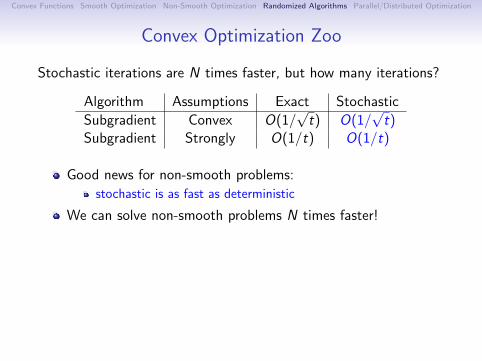

Convex Functions Smooth Optimization Non-Smooth Optimization Randomized Algorithms Parallel/Distributed Optimization
Deterministic vs. Stochastic Convergence Rates
Plot of convergence rates in smooth/strongly-convex case:
Stochastic vs. deterministic methods
• Goal = best of both worlds: linear rate with O(1) iteration cost
time
log(
exce
ss c
ost)
stochastic
deterministic

Convex Functions Smooth Optimization Non-Smooth Optimization Randomized Algorithms Parallel/Distributed Optimization
Speeding up Stochastic Gradient Methods
We can try accelerated/Newton-like stochastic methods:
These do not improve on the convergence rates.But may improve performance at start if noise is small.
Ideas that do improve convergence: averaging and large steps:
αt = O(1/tα) for α ∈ (0.5, 1) more robust than O(1/t).[Bach & Moulines, 2011]
Gradient averaging improves constants (‘dual averaging’).[Nesterov, 2007]
Averaging later iterations gives rates without smoothness.[Rakhlin et al., 2011]
Averaging in smooth case achieves same asymptotic rate asoptimal stochastic Newton method.[Polyak & Juditsky, 1992]]
Constant step-size α achieves rate of O(ρt) + O(α).[Nedic & Bertsekas, 2000]
Averaging and constant step-size achieves O(1/t) rate forstochastic Newton-like methods without strong convexity.[Bach & Moulines, 2013]

Convex Functions Smooth Optimization Non-Smooth Optimization Randomized Algorithms Parallel/Distributed Optimization
Motivation for Hybrid Methods for Smooth Problems
Stochastic vs. deterministic methods
• Goal = best of both worlds: linear rate with O(1) iteration cost
time
log(
exce
ss c
ost)
stochastic
deterministic

Convex Functions Smooth Optimization Non-Smooth Optimization Randomized Algorithms Parallel/Distributed Optimization
Motivation for Hybrid Methods for Smooth Problems
Stochastic vs. deterministic methods
• Goal = best of both worlds: linear rate with O(1) iteration cost
hybridlog(
exce
ss c
ost)
stochastic
deterministic
time

Convex Functions Smooth Optimization Non-Smooth Optimization Randomized Algorithms Parallel/Distributed Optimization
Stochastic Average Gradient
Should we use stochastic methods for smooth problems?
Can we have a rate of O(ρt) with only 1 gradientevaluation per iteration?
YES! The stochastic average gradient (SAG) algorithm:
Randomly select i(t) from 1, 2, . . . , n and compute f ′i(t)(xt).
x t+1 = x t − αt
N
N∑i=1
∇fi (x t)
Memory: y ti = ∇fi (x t) from the last t where i was selected.
[Le Roux et al., 2012]
Stochastic variant of increment average gradient (IAG).[Blatt et al., 2007]
Assumes gradients of non-selected examples don’t change.Assumption becomes accurate as ||x t+1 − x t || → 0.Memory requirements reduced to O(N) for many problems.

Convex Functions Smooth Optimization Non-Smooth Optimization Randomized Algorithms Parallel/Distributed Optimization
Stochastic Average Gradient
Should we use stochastic methods for smooth problems?
Can we have a rate of O(ρt) with only 1 gradientevaluation per iteration?
YES!
The stochastic average gradient (SAG) algorithm:
Randomly select i(t) from 1, 2, . . . , n and compute f ′i(t)(xt).
x t+1 = x t − αt
N
N∑i=1
∇fi (x t)
Memory: y ti = ∇fi (x t) from the last t where i was selected.
[Le Roux et al., 2012]
Stochastic variant of increment average gradient (IAG).[Blatt et al., 2007]
Assumes gradients of non-selected examples don’t change.Assumption becomes accurate as ||x t+1 − x t || → 0.Memory requirements reduced to O(N) for many problems.
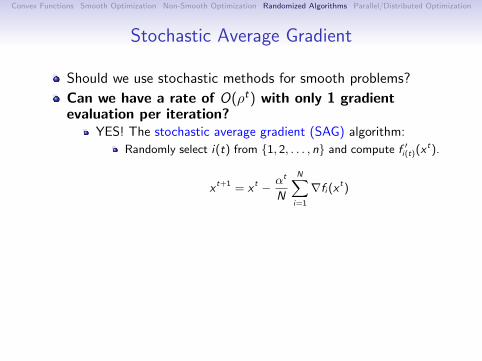
Convex Functions Smooth Optimization Non-Smooth Optimization Randomized Algorithms Parallel/Distributed Optimization
Stochastic Average Gradient
Should we use stochastic methods for smooth problems?
Can we have a rate of O(ρt) with only 1 gradientevaluation per iteration?
YES! The stochastic average gradient (SAG) algorithm:
Randomly select i(t) from 1, 2, . . . , n and compute f ′i(t)(xt).
x t+1 = x t − αt
N
N∑i=1
∇fi (x t)
Memory: y ti = ∇fi (x t) from the last t where i was selected.
[Le Roux et al., 2012]
Stochastic variant of increment average gradient (IAG).[Blatt et al., 2007]
Assumes gradients of non-selected examples don’t change.Assumption becomes accurate as ||x t+1 − x t || → 0.Memory requirements reduced to O(N) for many problems.

Convex Functions Smooth Optimization Non-Smooth Optimization Randomized Algorithms Parallel/Distributed Optimization
Stochastic Average Gradient
Should we use stochastic methods for smooth problems?
Can we have a rate of O(ρt) with only 1 gradientevaluation per iteration?
YES! The stochastic average gradient (SAG) algorithm:
Randomly select i(t) from 1, 2, . . . , n and compute f ′i(t)(xt).
x t+1 = x t − αt
N
N∑i=1
∇fi (x t)
Memory: y ti = ∇fi (x t) from the last t where i was selected.
[Le Roux et al., 2012]
Stochastic variant of increment average gradient (IAG).[Blatt et al., 2007]
Assumes gradients of non-selected examples don’t change.Assumption becomes accurate as ||x t+1 − x t || → 0.Memory requirements reduced to O(N) for many problems.
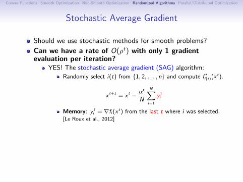
Convex Functions Smooth Optimization Non-Smooth Optimization Randomized Algorithms Parallel/Distributed Optimization
Stochastic Average Gradient
Should we use stochastic methods for smooth problems?
Can we have a rate of O(ρt) with only 1 gradientevaluation per iteration?
YES! The stochastic average gradient (SAG) algorithm:
Randomly select i(t) from 1, 2, . . . , n and compute f ′i(t)(xt).
x t+1 = x t − αt
N
N∑i=1
y ti
Memory: y ti = ∇fi (x t) from the last t where i was selected.
[Le Roux et al., 2012]
Stochastic variant of increment average gradient (IAG).[Blatt et al., 2007]
Assumes gradients of non-selected examples don’t change.Assumption becomes accurate as ||x t+1 − x t || → 0.Memory requirements reduced to O(N) for many problems.
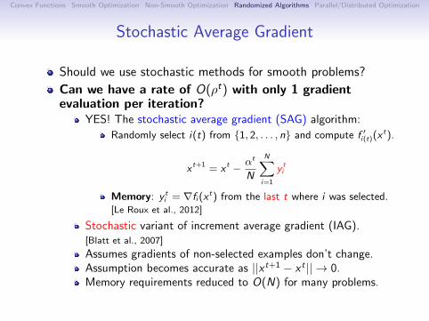
Convex Functions Smooth Optimization Non-Smooth Optimization Randomized Algorithms Parallel/Distributed Optimization
Stochastic Average Gradient
Should we use stochastic methods for smooth problems?
Can we have a rate of O(ρt) with only 1 gradientevaluation per iteration?
YES! The stochastic average gradient (SAG) algorithm:
Randomly select i(t) from 1, 2, . . . , n and compute f ′i(t)(xt).
x t+1 = x t − αt
N
N∑i=1
y ti
Memory: y ti = ∇fi (x t) from the last t where i was selected.
[Le Roux et al., 2012]
Stochastic variant of increment average gradient (IAG).[Blatt et al., 2007]
Assumes gradients of non-selected examples don’t change.Assumption becomes accurate as ||x t+1 − x t || → 0.Memory requirements reduced to O(N) for many problems.

Convex Functions Smooth Optimization Non-Smooth Optimization Randomized Algorithms Parallel/Distributed Optimization
Convex Optimization Zoo
Algorithm Rate Grads
Stochastic Gradient O(1/t) 1Gradient O((1− µ/L)t) N
SAG O((1−min µ16Li
, 18N )t) 1
Li is the Lipschitz constant over all ∇fi (Li ≥ L).
SAG has a similar speed to the gradient method, but onlylooks at one training example per iteration.
Recent work extends this result in various ways:
Similar rates for stochastic dual coordinate ascent.[Shalev-Schwartz & Zhang, 2013]
Memory-free variants. [Johnson & Zhang, 2013, Madavi et al., 2013]
Proximal-gradient variants. [Mairal, 2013]
ADMM variants. [Wong et al., 2013]
Improved constants. [Defazio et al., 2014]
Non-uniform sampling. [Schmidt et al., 2013]
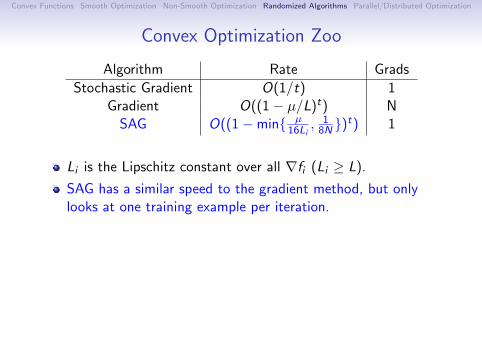
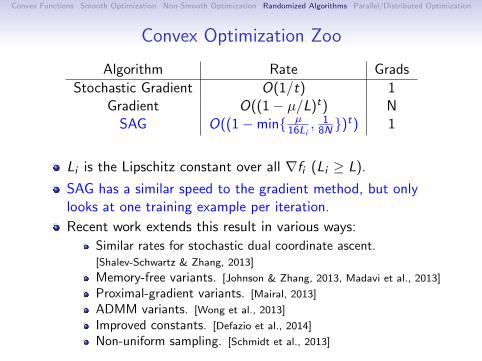

Convex Functions Smooth Optimization Non-Smooth Optimization Randomized Algorithms Parallel/Distributed Optimization
Comparing FG and SG Methods
quantum (n = 50000, p = 78) and rcv1 (n = 697641,p = 47236)
0 10 20 30 40 50
10−6
10−4
10−2
100
Effective Passes
Ob
jec
tiv
e m
inu
s O
ptim
um
AFG
L−BFGS
SGASG
IAG
0 10 20 30 40 50
10−4
10−3
10−2
10−1
100
Effective Passes
Ob
jec
tiv
e m
inu
s O
ptim
um
AFG
L−BFGS
SG
ASG
IAG

Convex Functions Smooth Optimization Non-Smooth Optimization Randomized Algorithms Parallel/Distributed Optimization
SAG Compared to FG and SG Methods
quantum (n = 50000, p = 78) and rcv1 (n = 697641,p = 47236)
0 10 20 30 40 50
10−12
10−10
10−8
10−6
10−4
10−2
100
Effective Passes
Ob
jec
tiv
e m
inu
s O
ptim
um
AFG
L−BFGS
SG
ASG
IAG
SAG−LS
0 10 20 30 40 50
10−15
10−10
10−5
100
Effective Passes
Ob
jec
tiv
e m
inu
s O
ptim
um
AFGL−BFGS
SG
ASG
IAG
SAG−LS

Convex Functions Smooth Optimization Non-Smooth Optimization Randomized Algorithms Parallel/Distributed Optimization
Coordinate Descent Methods
Consider problems of the form
minx
f (Ax) +n∑
i=1
hi (xi ), minx
∑
i∈Vfi (xi ) +
∑
(i ,j)∈E
fij(xi , xj),
where f and fij are smooth and G = V, E is a graph.
Appealing strategy for these problems is coordinate descent:
xj+ = xj − α∇j f (x).
(i.e., update one variable at a time)
We can typically perform a cheap and precise line-search for α.
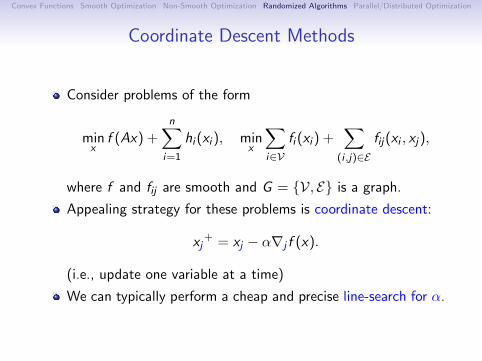

Convex Functions Smooth Optimization Non-Smooth Optimization Randomized Algorithms Parallel/Distributed Optimization
Convergence Rate of Coordinate DescentThe steepest descent choice is j = argmaxj|∇j f (x)|.
(but only efficient to calculate in some special cases)
Convergence rate (strongly-convex, gradient is L-Lipschitz):
O((1− µ/LD)t)
This L is typically much smaller than L across all coordinates:Coordinate descent if we can do D coordinate descent stepsfor cost of one gradient step.
Choosing a random coordinate j has same rate as steepestcoordinate descent.[Nesterov, 2010]
Various extensions:Non-uniform sampling (Lipschitz sampling) [Nesterov, 2010]
Projected coordinate descent (product constraints)[Nesterov, 2010]
Proximal coordinate descent (separable non-smooth term)Richtarik & Takac, 2011]
Frank-Wolfe coordinate descent (product constraints)[LaCoste-Julien et al., 2013]
Accelerated version [Fercoq & Richtarik, 2013]
(exact step size for `1-regularized least squares)
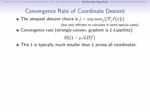
Convex Functions Smooth Optimization Non-Smooth Optimization Randomized Algorithms Parallel/Distributed Optimization
Convergence Rate of Coordinate DescentThe steepest descent choice is j = argmaxj|∇j f (x)|.
(but only efficient to calculate in some special cases)
Convergence rate (strongly-convex, gradient is L-Lipschitz):
O((1− µ/LD)t)
This L is typically much smaller than L across all coordinates:
Coordinate descent if we can do D coordinate descent stepsfor cost of one gradient step.
Choosing a random coordinate j has same rate as steepestcoordinate descent.[Nesterov, 2010]
Various extensions:Non-uniform sampling (Lipschitz sampling) [Nesterov, 2010]
Projected coordinate descent (product constraints)[Nesterov, 2010]
Proximal coordinate descent (separable non-smooth term)Richtarik & Takac, 2011]
Frank-Wolfe coordinate descent (product constraints)[LaCoste-Julien et al., 2013]
Accelerated version [Fercoq & Richtarik, 2013]
(exact step size for `1-regularized least squares)

Convex Functions Smooth Optimization Non-Smooth Optimization Randomized Algorithms Parallel/Distributed Optimization
Convergence Rate of Coordinate DescentThe steepest descent choice is j = argmaxj|∇j f (x)|.
(but only efficient to calculate in some special cases)
Convergence rate (strongly-convex, gradient is L-Lipschitz):
O((1− µ/LD)t)
This L is typically much smaller than L across all coordinates:Coordinate descent if we can do D coordinate descent stepsfor cost of one gradient step.
Choosing a random coordinate j has same rate as steepestcoordinate descent.[Nesterov, 2010]
Various extensions:Non-uniform sampling (Lipschitz sampling) [Nesterov, 2010]
Projected coordinate descent (product constraints)[Nesterov, 2010]
Proximal coordinate descent (separable non-smooth term)Richtarik & Takac, 2011]
Frank-Wolfe coordinate descent (product constraints)[LaCoste-Julien et al., 2013]
Accelerated version [Fercoq & Richtarik, 2013]
(exact step size for `1-regularized least squares)

Convex Functions Smooth Optimization Non-Smooth Optimization Randomized Algorithms Parallel/Distributed Optimization
Convergence Rate of Coordinate DescentThe steepest descent choice is j = argmaxj|∇j f (x)|.
(but only efficient to calculate in some special cases)
Convergence rate (strongly-convex, gradient is L-Lipschitz):
O((1− µ/LD)t)
This L is typically much smaller than L across all coordinates:Coordinate descent if we can do D coordinate descent stepsfor cost of one gradient step.
Choosing a random coordinate j has same rate as steepestcoordinate descent.[Nesterov, 2010]
Various extensions:Non-uniform sampling (Lipschitz sampling) [Nesterov, 2010]
Projected coordinate descent (product constraints)[Nesterov, 2010]
Proximal coordinate descent (separable non-smooth term)Richtarik & Takac, 2011]
Frank-Wolfe coordinate descent (product constraints)[LaCoste-Julien et al., 2013]
Accelerated version [Fercoq & Richtarik, 2013]
(exact step size for `1-regularized least squares)
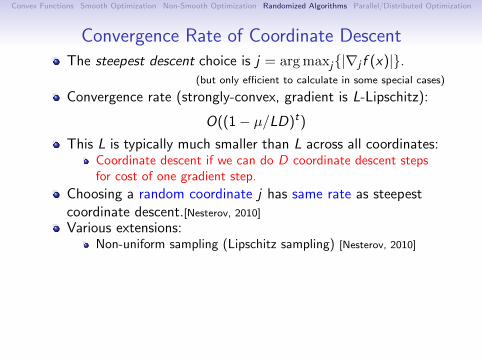
Convex Functions Smooth Optimization Non-Smooth Optimization Randomized Algorithms Parallel/Distributed Optimization
Convergence Rate of Coordinate DescentThe steepest descent choice is j = argmaxj|∇j f (x)|.
(but only efficient to calculate in some special cases)
Convergence rate (strongly-convex, gradient is L-Lipschitz):
O((1− µ/LD)t)
This L is typically much smaller than L across all coordinates:Coordinate descent if we can do D coordinate descent stepsfor cost of one gradient step.
Choosing a random coordinate j has same rate as steepestcoordinate descent.[Nesterov, 2010]
Various extensions:Non-uniform sampling (Lipschitz sampling) [Nesterov, 2010]
Projected coordinate descent (product constraints)[Nesterov, 2010]
Proximal coordinate descent (separable non-smooth term)Richtarik & Takac, 2011]
Frank-Wolfe coordinate descent (product constraints)[LaCoste-Julien et al., 2013]
Accelerated version [Fercoq & Richtarik, 2013]
(exact step size for `1-regularized least squares)
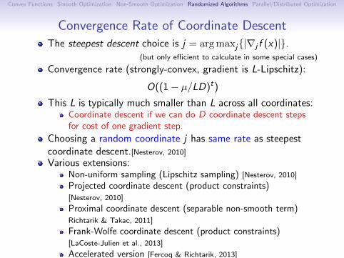
Convex Functions Smooth Optimization Non-Smooth Optimization Randomized Algorithms Parallel/Distributed Optimization
Convergence Rate of Coordinate DescentThe steepest descent choice is j = argmaxj|∇j f (x)|.
(but only efficient to calculate in some special cases)
Convergence rate (strongly-convex, gradient is L-Lipschitz):
O((1− µ/LD)t)
This L is typically much smaller than L across all coordinates:Coordinate descent if we can do D coordinate descent stepsfor cost of one gradient step.
Choosing a random coordinate j has same rate as steepestcoordinate descent.[Nesterov, 2010]
Various extensions:Non-uniform sampling (Lipschitz sampling) [Nesterov, 2010]
Projected coordinate descent (product constraints)[Nesterov, 2010]
Proximal coordinate descent (separable non-smooth term)Richtarik & Takac, 2011]
Frank-Wolfe coordinate descent (product constraints)[LaCoste-Julien et al., 2013]
Accelerated version [Fercoq & Richtarik, 2013]
(exact step size for `1-regularized least squares)

Convex Functions Smooth Optimization Non-Smooth Optimization Randomized Algorithms Parallel/Distributed Optimization
Randomized Linear Algebra
Consider problems of the form
minx
f (Ax),
where bottleneck is matrix multiplication and A is low-rank.
Randomized linear algebra approaches uses
A ≈ Q(QTA),
or choses random row/columns subsets.
Now work with f (Q(QTA)).
Q formed from Gram-Schmidt and matrix multiplication withrandom vectors gives very good approximation bounds, ifsingular values decay quickly.[Halko et al., 2011, Mahoney, 2011]
May work quite badly if singular values decay slowly.
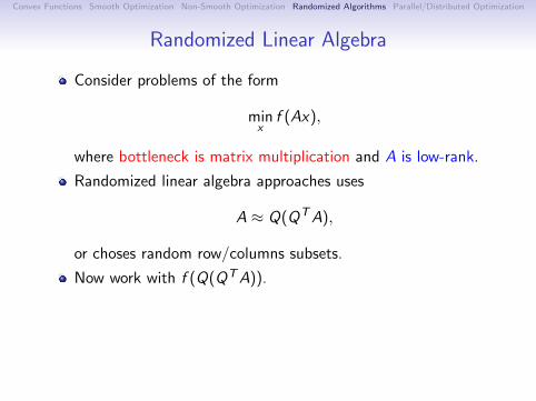

Convex Functions Smooth Optimization Non-Smooth Optimization Randomized Algorithms Parallel/Distributed Optimization
Outline
1 Convex Functions
2 Smooth Optimization
3 Non-Smooth Optimization
4 Randomized Algorithms
5 Parallel/Distributed Optimization

Convex Functions Smooth Optimization Non-Smooth Optimization Randomized Algorithms Parallel/Distributed Optimization
Motivation for Parallel and Distributed
Two recent trends:
We aren’t making large gains in serial computation speed.Datasets no longer fit on a single machine.
Result: we must use parallel and distributed computation.
Two major issues:
Synchronization: we can’t wait for the slowest machine.Communication: we can’t transfer all information.
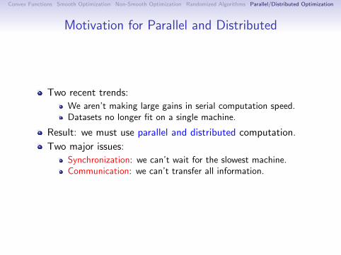

Convex Functions Smooth Optimization Non-Smooth Optimization Randomized Algorithms Parallel/Distributed Optimization
Embarassing Parallelism in Machine Learning
A lot of machine learning problems are embarrassingly parallel:
Split task across M machines, solve independently, combine.
E.g., computing the gradient in deterministic gradient method,
1
N
N∑
i=1
∇fi (x) =1
N
N/M∑
i=1
∇fi (x) +
2N/M∑
i=(N/M)+1
∇fi (x) + . . .
.
These allow optimal linear speedups.
You should always consider this first!

Convex Functions Smooth Optimization Non-Smooth Optimization Randomized Algorithms Parallel/Distributed Optimization
Asynchronous Computation
Do we have to wait for the last computer to finish?
No!
Updating asynchronously saves a lot of time.
E.g., stochastic gradient method on shared memory:
xk+1 = xk − α∇fik (xk−m).
You need to decrease step-size in proportion to asynchrony.
Convergence rate decays elegantly with delay m.[Niu et al., 2011]
Convex Functions Smooth Optimization Non-Smooth Optimization Randomized Algorithms Parallel/Distributed Optimization
Reduced Communication: Parallel Coordinate Descnet
It may be expensive to communicate parameters x .
One solution: use parallel coordinate descent:
xj1 = xj1 − αj1∇j1f (x)
xj2 = xj2 − αj2∇j2f (x)
xj3 = xj3 − αj3∇j3f (x)
Only needs to communicate single coordinates.
Again need to decrease step-size for convergence.
Speedup is based on density of graph.[Richtarik & Takac, 2013]
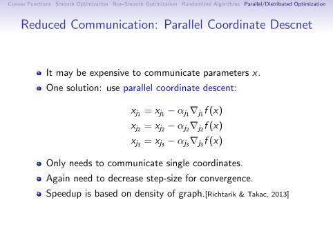

Convex Functions Smooth Optimization Non-Smooth Optimization Randomized Algorithms Parallel/Distributed Optimization
Reduced Communication: Decentralized Gradient
We may need to distribute the data across machines.
We may not want to update a ‘centralized’ vector x .
One solution: decentralized gradient method:Each processor has its own data samples f1, f2, . . . fm.Each processor has its own parameter vector xc .Each processor only communicates with a limited number ofneighbours nei(c).
xc =1
|nei(c)|∑
c ′∈nei(c)
xc −αc
M
M∑
i=1
∇fi (xc).
Gradient descent is special case where all neighbourscommunicate.
With modified update, rate decays gracefully as graphbecomes sparse.[Shi et al., 2014]
Can also consider communication failures.[Agarwal & Duchi, 2011]
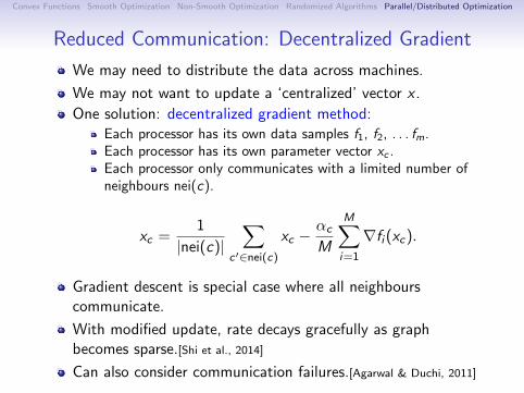

Convex Functions Smooth Optimization Non-Smooth Optimization Randomized Algorithms Parallel/Distributed Optimization
Summary
Summary:
Part 1: Convex functions have special properties that allow usto efficiently minimize them.
Part 2: Gradient-based methods allow elegant scaling withproblems sizes for smooth problems.
Part 3: Tricks like proximal-gradient methods allow the samescaling for many non-smooth problems.
Part 4: Randomized algorithms allow even further scaling forproblem structures that commonly arise in machine learning.
Part 5: The future will require parallel and distributed that areasynchronous and are careful about communication costs.
Thank you for coming and staying until the end!