General rights Copyright and moral rights for the publications made accessible in the public portal are retained by the authors and/or other copyright owners and it is a condition of accessing publications that users recognise and abide by the legal requirements associated with these rights.

Users may download and print one copy of any publication from the public portal for the purpose of private study or research.

You may not further distribute the material or use it for any profit-making activity or commercial gain

You may freely distribute the URL identifying the publication in the public portal If you believe that this document breaches copyright please contact us providing details, and we will remove access to the work immediately and investigate your claim.

Downloaded from orbit.dtu.dk on: Feb 07, 2022

Convex Relaxations of Chance Constrained AC Optimal Power Flow

Venzke, Andreas; Halilbasic, Lejla; Markovic, Uros; Hug, Gabriela; Chatzivasileiadis, Spyros

Published in:IEEE Transactions on Power Systems

Link to article, DOI:10.1109/TPWRS.2017.2760699

Publication date:2017

Document VersionPeer reviewed version

Link back to DTU Orbit

Citation (APA):Venzke, A., Halilbasic, L., Markovic, U., Hug, G., & Chatzivasileiadis, S. (2017). Convex Relaxations of ChanceConstrained AC Optimal Power Flow. IEEE Transactions on Power Systems, 33(3), 2829 - 2841.https://doi.org/10.1109/TPWRS.2017.2760699

ACCEPTED FOR PUBLICATION IN IEEE TRANSACTIONS ON POWER SYSTEMS 1

Convex Relaxations of Chance ConstrainedAC Optimal Power Flow

Andreas Venzke, Student Member, IEEE, Lejla Halilbasic, Student Member, IEEE, Uros Markovic, StudentMember, IEEE, Gabriela Hug, Senior Member, IEEE, and Spyros Chatzivasileiadis, Member, IEEE

Abstract—High penetration of renewable energy sources andthe increasing share of stochastic loads require the explicit repre-sentation of uncertainty in tools such as the optimal power flow(OPF). Current approaches follow either a linearized approach oran iterative approximation of non-linearities. This paper proposesa semidefinite relaxation of a chance constrained AC-OPF whichis able to provide guarantees for global optimality. Using apiecewise affine policy, we can ensure tractability, accuratelymodel large power deviations, and determine suitable correctivecontrol policies for active power, reactive power, and voltage.We state a tractable formulation for two types of uncertaintysets. Using a scenario-based approach and making no priorassumptions about the probability distribution of the forecasterrors, we obtain a robust formulation for a rectangular uncer-tainty set. Alternatively, assuming a Gaussian distribution of theforecast errors, we propose an analytical reformulation of thechance constraints suitable for semidefinite programming. Wedemonstrate the performance of our approach on the IEEE 24and 118 bus system using realistic day-ahead forecast data andobtain tight near-global optimality guarantees.

Index Terms—AC optimal power flow, convex optimization,chance constraints, semidefinite programming, uncertainty.

I. INTRODUCTION

POWER system operators have to deal with higher degreesof uncertainty in operation and planning. If uncertainty is

not explicitly considered, increasing shares of unpredictablerenewable generation and stochastic loads, such as electricvehicles, can lead to higher costs and jeopardize systemsecurity. The scope of this work is to introduce a convexAC optimal power flow (OPF) formulation which is able toaccurately model the effect of forecast errors on the powerflow, can define a-priori suitable corrective control policiesfor active power, reactive power, and voltage, and can providenear-global optimality guarantees.

Chance constraints are included in the OPF formulationto account for uncertainty in power injections, defining amaximum allowable probability of constraint violation. It isgenerally agreed that the non-linear nature of the AC-OPFalong with the probabilistic constraints render the problem formost instances intractable [1]. To ensure tractability of theseconstraints, either a data-driven or scenario-based approach isapplied, or the assumption of specific uncertainty distributionsis required for an analytical reformulation of the chanceconstraints. To deal with the higher complexity of chance

A. Venzke, L. Halilbasic and S. Chatzivasileiadis are with the Departmentof Electrical Engineering, Technical University of Denmark, Kongens Lyngby,Denmark.

U. Markovic and G. Hug are with the Power Systems Laboratory, ETHZurich, Zurich, Switzerland.

constrained OPF, existing approaches either assume a DC-OPF [2]–[6], a linearized AC-OPF [7]–[10] or solve iterativelylinearized instances of the non-linear AC-OPF [11], [12].Chance constrained DC-OPF results to a faster and morescalable algorithm, but it is an approximation that neglectslosses, reactive power, and voltage constraints, and can exhibitsubstantial approximation errors [13].

Refs. [2] and [3] formulate a chance constrained DC-OPF assuming a Gaussian distribution of the forecast errors.The work in [2] relies on a cutting-plane algorithm to solvethe resulting optimization problem, whereas the work in [3]states a direct analytical reformulation of the same chanceconstraints. This framework is further extended by the workin [4] which assumes uncertainty sets for both the mean andthe variance of the underlying Gaussian distributions to obtaina more distributionally robust formulation. The work in [5]formulates a robust multi-period chance constrained DC-OPFassuming interval bounds on uncertain wind infeeds. Theseworks [2]–[5] include corrective control of the generation unitsto restore the active power system balance as a function of theforecast errors. The work in [6] extends this corrective controlframework to include HVDC converter active power set-pointsand phase shifting transformers in an N-1 security context.

Alternatively, the works in [7]–[10] use a linearization of theAC power flow equations based on [14] to achieve a tractableformulation of the chance constraints. As the operating pointis not known a-priori, the linearization is performed arounda flat start or no-load voltage, and not the actual operatingpoint. These works [7]–[10] focus on low-voltage distributionsystems with high share of photovoltaic (PV) production andminimize PV curtailment subject to chance constraints onvoltage magnitudes. Scenario-based methods are applied toachieve a tractable formulation. In this framework, line flowlimits and corrective control from conventional generation arenot considered. Furthermore, the utilized linearization in [7]–[10] is designed for radial distribution grids and assumes novoltage control capability of generation units.

In Ref. [11], an iterative back-mapping and linearization ofthe full AC power flow equations is used to solve the chanceconstrained AC-OPF. The recent work in [12] uses an iterativeprocedure to calculate the full Jacobian, which is the exact ACpower flow linearization around the operating point. Assuminga Gaussian distribution of the forecast errors, an analyticalreformulation of the chance constraints on voltage magnitudeand current line flow is proposed. Although this approach canbe shown to scale well, it is not convex and does not guaranteeconvergence.

ACCEPTED FOR PUBLICATION IN IEEE TRANSACTIONS ON POWER SYSTEMS 2

(I) Non-convexAC-OPF

(II) Non-convex chanceconstrained AC-OPF

(III) Non-convex chanceconstrained AC-OPFusing affine policy

(IV) Convex chanceconstrained AC-OPFusing affine policy

relaxation gap

remove

rank-1

parametrize solution space

Fig. 1. We restrict the solution space of the non-linear chance constrainedAC-OPF to the parametrization by the affine policy. This problem is relaxedby dropping the non-convex rank constraint. With relaxation gap we refer tothe gap between problems (IV) and (III).

In this work, we formulate convex relaxations of chanceconstrained AC-OPF which allow us to provide guaranteesfor the optimality of the solution, or otherwise upper-boundthe distance to the global optimum of the original non-linearproblem. Besides that, we include chance constraints for allrelevant state variables, namely active and reactive power,voltage magnitudes and active and apparent branch flows. Twotractable formulations of the chance constraints are proposed.First, based on realistic forecast data and making no priorassumptions about the probability distributions, we formulatea rectangular uncertainty set and, subsequently, the associatedchance constraints. Second, assuming a Gaussian distributionof the forecast errors, we provide an analytical reformulationof the chance constraints.

A. Convex Relaxations and Relaxation Gap

In general, the AC-OPF is a non-convex, non-linear prob-lem. As a result, identified solutions are not guaranteed tobe globally optimal and the distance to the global optimumcannot be specified. Recent advancements in the area ofconvex optimization with polynomials have achieved to relaxthe non-linear, non-convex optimal power flow problem andtransform it to a convex semidefinite (SDP) or second-ordercone problem [15]–[17]. Formulating a convex optimizationproblem results in tractable solution algorithms that can deter-mine the global minimum. Within power systems, finding theglobal minimum has two important implications. First, froman economic point of view, it can result to substantial costsavings [18]. Second, from a technical point of view, the globaloptimum determines a lower or an upper bound of the requiredcontrol effort. The term relaxation gap denotes the differencebetween the minimum obtained through the convex relaxationand the global minimum of the original non-convex problem.A relaxation is tight, if the relaxation gap is small. A relaxationis exact, if the relaxation gap is zero, i.e. zero relaxationgap is achieved when the minimum of the convex relaxationcoincides with the global minimum of the original non-convex,non-linear problem. Since the work in [19] has shown cases inwhich the semidefinite relaxation of [15] fails, it is necessaryto investigate the relaxation gap of the obtained solution,and examine the conditions under which we can obtain zerorelaxation gap. In the work [20] a reactive power penalty isintroduced, which allows to upper bound the distance to global

optimum. In this work, we develop a penalized semidefiniteformulation for a chance constrained AC-OPF, which allowsus as well to determine an upper bound of the distance tothe global optimum. In Fig. 1 we illustrate the previouslyexplained concepts in the context of our work. With relaxationgap, we refer to the gap between the semidefinite relaxationand a non-linear chance constrained AC-OPF which uses theaffine policy to parametrize the solution space.

B. Main Contributions

In this work we propose a framework for a convex chanceconstrained AC-OPF. The work in [21] makes a first steptowards such a formulation which takes into account securityconstraints and uncertainty. The change of the system state isdescribed with an affine policy as an explicit function of theforecast errors. A combination of the scenario approach androbust optimization is used to ensure tractability of the chanceconstraints [22]. For the convex relaxations we build upon theSDP AC-OPF formulation proposed in [15]. The contributionsof our work are the following:• To the best of our knowledge, this is the first paper that

proposes a convex formulation for the chance constrainedOPF that (a) is able to determine if it has found the globalminimum of the original non-convex problem1, and (b)if not, it is able to determine the distance to the globalminimum through the relaxation gap.

• In this paper, we introduce a penalty term on powerlosses which allows us to obtain near-global optimalityguarantees and we investigate the conditions under whichwe can obtain a zero relaxation gap.We show that thispenalty term is small in practice, leading to tight near-global optimality guarantees of the obtained solution.

• We formulate tractable chance constraints suitable forsemidefinite programming for two types of uncertaintysets. First, using a piecewise affine policy, we state atractable formulation of the chance constrained AC-OPFwith convex relaxations that makes no prior assumptionson the type of probability distribution. Using existingdata or scenarios, we determine a rectangular uncertaintyset; as the set and the chance constraints are affine orconvex, we can account for the whole set by enforcingthe chance constraints only at its vertices [22]. Second,assuming Gaussian distributions, we formulate tractablechance constraints for the optimal power flow equationsthat are suitable for semidefinite programming. In that,we also assume the correlation of different uncertainvariables. To the best of our knowledge, this is the firstpaper that introduces a tractable reformulation of thechance constrained AC-OPF with convex relaxations forGaussian distributions.

• The proposed framework includes corrective control poli-cies related to active and reactive power, and voltage.

• Based on realistic forecast data and the IEEE 118 bus testcase, we compare our approach for both uncertainty setsto the chance constrained DC-OPF formulation in [5],

1As we will discuss later in this paper, in cases where a penalized SDPformulation is necessary, this point corresponds to a near-global minimum.

ACCEPTED FOR PUBLICATION IN IEEE TRANSACTIONS ON POWER SYSTEMS 3

and the iterative AC-OPF in [12]. Compared to the DC-OPF formulation, we find that the formulations proposedin this paper are more accurate and significantly decreaseconstraint violations. For the rectangular uncertainty set,the affine policy complies with all considered chanceconstraints and outperforms all other methods havingthe lowest number of constraint violations. At the sametime, we obtain tight near-global optimality guaranteeswhich ensure that the distance to the global optimum issmaller than 0.01% of the objective value. For a Gaussiandistribution, both the iterative AC-OPF and our approachsatisfy the constraint violation limit, with our approachachieving slightly lower costs due to the corrective con-trol capabilities. As the realistic forecast data we useddo not follow a Gaussian distribution, we also observedthat both approaches may exceed the constraint violationlimit at certain timesteps for that dataset.

The remainder of this work is structured as follows: InSection II the convex relaxation of the chance constrainedAC-OPF problem is formulated. Section III introduces thepiecewise affine policy, defines corrective control policies andstates the tractable OPF formulation for both uncertainty sets.Section IV states an alternative approach using a linearizationbased on power transfer distribution factors (PTDFs). Sec-tion V investigates the relaxation gap for a IEEE 24 bus systemand presents numerical results for a IEEE 118 bus systemusing realistic forecast data. Section VI concludes the paper.The nomenclature is provided in Table I. An underline andoverline denote, respectively, the upper and lower bound of avariable.

II. OPTIMAL POWER FLOW FORMULATION

A. Convex Relaxation of AC Optimal Power Flow

For completeness, we outline the semidefinite relaxationof the AC-OPF problem as formulated in [15]. A powergrid consists of N buses and L lines. The set of generatorbuses is denoted with G. The following auxiliary variables areintroduced for each bus k ∈ N and line (l,m) ∈ L:

Yk := ekeTk Y (1)

Ylm := (ylm + ylm)eleTl − (ylm)ele

Tm (2)

Yk :=1

2

[<{Yk + Y Tk } ={Y Tk − Yk}={Yk − Y Tk } <{Yk + Y Tk }

](3)

Ylm :=1

2

[<{Ylm + Y Tlm} ={Y Tlm − Ylm}={Ylm − Y Tlm} <{Ylm + Y Tlm}

](4)

Yk :=−1

2

[={Yk + Y Tk } <{Yk − Y Tk }<{Y Tk − Yk} ={Yk + Y Tk }

](5)

Mk :=

[eke

Tk 0

0 ekeTk

](6)

X := [<{V}={V}]T (7)

Matrix Y denotes the bus admittance matrix of the power grid,ek the k-th basis vector, ylm the shunt admittance and ylm theseries admittance of line (l,m) ∈ L, and V the vector of

TABLE INOMENCLATURE

Power grid

N , L, G Set of buses, lines and generators in the power networkck2

, ck1, ck0

Quadratic, linear and constant cost term of generator kY Admittance matrixylm, ylm Shunt and series admittance of line (l,m)nb Number of buses in the power networkxlm Reactance of line (l,m)BAC Admittance matrix based on DC approximationPTDFlm Power transfer distribution factor for line (l,m)

Optimal power flow

PGk, QGk

Active and reactive power generation at bus kVk Voltage magnitude at bus kPlm, Slm Active and apparent branch flow on line (l,m)V Complex bus voltage vectorX Real and imaginary bus voltage vectorPDk

, QDkActive and reactive power consumption at bus k

W Matrix with product of voltagesW (ζi) Matrix W as a function of the forecast errorsW0 Matrix W for forecasted system stateBi System change for forecast error iBu

i , Bli System change for upper/lower limit on forecast error i

Wv Matrix W for vertex vρ Ratio of second to third eigenvalue of Wδopt Near-global optimality measure

Uncertainty modeling

nW , W Number of wind farms and set of buses with wind farmsPW Wind infeedsP fW Forecasted wind infeedsζ Wind forecast errorsε Maximum violation probability of chance constraintsdG Generator participation factorsdW Wind deviation vectorγ Slack variable on generator participation factorµ Weight for power loss penaltycos(φ) Power factor of wind farmsτ Ratio of maximum reactive to active powerNs Number of scenariosβ Confidence parameterv Vertices of rectangular uncertainty setnv , V Number and set of vertices vζv Forecast error for vertex v of uncertainty setΛ Covariance matrixλ, η Eigenvalues and eigenvectors of covariance matrixκ Limit on Gaussian forecast error

complex bus voltages. The non-linear AC-OPF problem canbe written using (1) – (7) as

minW

∑k∈G

{ck2(Tr{YkW}+ PDk)2 +

ck1(Tr{YkW}+ PDk) + ck0} (8)

subject to the following constraints for each bus k ∈ N andline (l,m) ∈ L:

PGk− PDk

≤ Tr{YkW} ≤ PGk− PDk

(9)

QGk−QDk

≤ Tr{YkW} ≤ QGk−QDk

(10)

V 2k ≤ Tr{MkW} ≤ V

2

k (11)

−P lm ≤ Tr{YlmW} ≤ P lm (12)

Tr{YlmW}2 + Tr{YlmW}2 ≤ S2

lm (13)

W = XXT (14)

ACCEPTED FOR PUBLICATION IN IEEE TRANSACTIONS ON POWER SYSTEMS 4

The objective (8) minimizes generation cost, where ck2, ck1

and ck0 are quadratic, linear and constant cost variablesassociated with power production of generator k ∈ G.2 Theterms PDk

and QDkdenote the active and reactive power

consumption at bus k. Constraints (9) and (10) include thenodal active and reactive power flow balances; PGk

, PGk,

QGk

and QGkare generator limits for minimum and maximum

active and reactive power, respectively. The bus voltages areconstrained by (11) with corresponding lower and upper limitsV k, V k. The active and apparent power branch flow Plm andSlm on line (l,m) ∈ L are limited by P lm (12) and Slm(13), respectively. To obtain an optimization problem linearin W , the objective function is reformulated using Schur’scomplement:

minW,α

∑k∈G

αk (15)[ck1Tr{YkW}+ ak

√ck2Tr{YkW}+ bk√

ck2Tr{YkW}+ bk −1

]� 0 (16)

where ak := −αk + ck0 + ck1PDkand bk :=

√ck2PDk

. Inaddition, the apparent branch flow constraint (13) is rewritten: −(Slm)2 Tr{YlmW} Tr{YlmW}

Tr{YlmW} −1 0Tr{YlmW} 0 −1

� 0 (17)

The non-convex constraint (14) can be expressed by:

W � 0 (18)rank(W ) = 1 (19)

The convex relaxation is introduced by dropping the rank con-straint (19), relaxing the non-linear, non-convex AC-OPF to aconvex semidefinite program (SDP). The work in [15] provesthat if the rank of W obtained from the SDP relaxation is 1,then W is the global optimum of the non-linear, non-convexAC-OPF and the optimal voltage vector can be computedfollowing the procedure described in [23].

B. Inclusion of Chance Constraints

Renewable energy sources and stochastic loads introduceuncertainty in power system operation. To account for uncer-tainty in bus power injections, we extend the presented OPFformulation with chance constraints. A number of nW windfarms are introduced in the power grid at buses k ∈ W andmodeled as

PWk= P fWk

+ ζk (20)

where PW are the actual wind infeeds, P fW are the forecastedvalues and ζ are the uncertain forecast errors. To simplifynotation, the resulting upper and lower bounds on net activeand reactive power injections are written in compact form as:

P k := PGk− PDk

+ P fWk+ ζk, (21)

P k := PGk− PDk

+ P fWk+ ζk (22)

Qk := QGk−QDk

(23)Qk

:= QGk−QDk

(24)

2In case renewable curtailment costs are assumed, this could introducenegative linear costs, which may not result in a tight relaxation.

The convex chance constrained AC-OPF problem includeschance constraints for each bus k ∈ N and line (l,m) ∈ L:

minW,α

∑k∈G

αk (25)

s.t. (9), (10), (11), (12), (17), (16), (18) for W = W0 (26)

P{P k ≤ Tr{YkW (ζ)} ≤ P k, (27)

Qk≤ Tr{YkW (ζ)} ≤ Qk, (28)

V 2k ≤ Tr{MkW (ζ)} ≤ V 2

k, (29)

− P lm ≤ Tr{YlmW (ζ)} ≤ P lm, (30)[−(Slm)2 Tr{YlmW (ζ)} Tr{YlmW (ζ)}

Tr{YlmW (ζ)} −1 0

Tr{YlmW (ζ)} 0 −1

]� 0, (31)

W (ζ) � 0}≥ 1− ε (32)

The parameter ε ∈ (0, 1) defines the upper bound on theviolation probability of the chance constraints (27) – (32).The function W (ζ) denotes the system state as a function ofthe forecast errors. The chance constrained AC-OPF problem(25) – (32) is an infinite-dimensional problem optimizing overW (ζ) which is a function of a continuous uncertain variableζ [21]. This renders the problem intractable, which makes itnecessary to identify a suitable approximation for W (ζ) [24].In the following, an approximation of an explicit dependenceof W (ζ) on the forecast errors is presented.

III. PIECEWISE AFFINE POLICY

We present a formulation of the chance constraints using apiecewise affine policy, which approximates the system changeas a linear function of the forecast errors. This allows usto include corrective control policies for active and reactivepower, and voltages. We propose a tractable formulation fortwo types of uncertainty sets. First, using an approach basedon randomized and robust optimization, and making no priorassumption on the underlying probability distributions, wedetermine a rectangular uncertainty set. For that, it is sufficientto enforce the chance constraints at its vertices. Second,assuming a Gaussian distribution of the forecast errors, wecan provide an analytical reformulation of the linear chanceconstraints and a suitable approximation of the semidefinitechance constraints.

A. Formulation of Chance Constraints

The main idea is to describe the matrix W (ζ) as the sumof the forecasted system operating state W0 and the changeof the system state Bi due to each forecast error. Similar to[21], the matrix W (ζ) is approximated using the affine policy

W (ζ) = W0 +

nw∑i=1

ζiBi (33)

where W0 and Bi are matrices modeled as decision variables.Eq. (33) provides an affine parametrization of the solutionspace for the product of real and imaginary part of bus voltagesdescribed by W (ζ). The main advantages of the affine policyare that it resembles affine corrective control policies and

ACCEPTED FOR PUBLICATION IN IEEE TRANSACTIONS ON POWER SYSTEMS 5

naturally allows to include these as well. Furthermore, as thesystem change depends linearly on the forecast error, in case aGaussian distribution is assumed, an analytical reformulationcan be applied as we will show in Section III-E. Inserting (33)in (27) – (32) yields:

P{P k ≤ Tr{YkW0}+

nw∑i

ζiTr{YkBi} ≤ P k (34)

Qk≤ Tr{YkW0}+

nw∑i

ζiTr{YkBi} ≤ Qk (35)

V 2k ≤ Tr{MkW0}+

nw∑i

ζiTr{MkBi} ≤ V2

k (36)

− P lm ≤ Tr{YlmW0}+

nw∑i

ζiTr{YlmBi} ≤ P lm (37)−S2

lm ΞPlm ΞQlmΞPlm −1 0

ΞQlm 0 −1

� 0 (38)

W0 +

nw∑i

ζiBi � 0}≥ 1− ε (39)

The terms ΞPlm := Tr{YlmW0} +∑nW

i=1 ζiTr{YlmBi} andΞQlm := Tr{YlmW0} +

∑nW

i=1 ζiTr{YlmBi} denote the activeand reactive power flow on transmission line (l,m) ∈ L as afunction of the forecast errors. Note that the chance constraints(34) – (39) are convex and can be classified in two groups: Theconstraints (34) – (37) are linear scalar chance constraints andthe constraints (38) – (39) are semidefinite chance constraints.

B. Corrective Control Policies

The affine policy allows to include corrective control poli-cies related to active power, reactive power, and voltage in theAC-OPF formulation. In this work, the implemented policiesare generator active power control, generator voltage control,and wind farm reactive power control.

Throughout the transmission system operation, generationhas to match demand and system losses. If an imbalance oc-curs, automatic generation control (AGC) restores the systembalance [25]. Hence, designated generators in the power gridwill respond to changes in wind power by adjusting theiroutput as part of secondary frequency control. The generatorparticipation factors are defined in the vector dG ∈ Rnb . Theterm nb denotes the number of buses. The sum of the changein generator active power set-points should compensate thedeviation in wind generation, i. e.

∑k∈G dGk

= 1. The windvector diW ∈ Rnb for each wind feed-in i in [1, nW ] has a{−1} entry corresponding to the bus where the i-th wind farmis located at. The other entries are zero. The line losses ofthe AC power grid vary non-linearly with changes in windinfeeds. To compensate for this change in system losses, weadd a slack variable γi to the generator set-points. This resultsin the following constraints on each matrix Bi, bus k ∈ Nand wind feed-in i in [1, nW ]:

Tr{YkBi} = dGk(1 + γi) + diWk

(40)

As a result of (40), it is ensured that each generator compen-sates the non-linear change in system losses according to its

participation factor. To constrain the magnitude of the slackvariable, a penalty term is added to the objective function (25),where the term µ ≥ 0 is a penalty weight:

minW,α, γ

∑k∈G

αk + µ

nw∑i

γi (41)

This penalty guides the optimization to a physically mean-ingful solution, i.e. it allows us to obtain rank-1 solutionmatrices. The increase in losses due to deviations in wind in-feeds is minimized. With this penalized semidefinite AC-OPFformulation, near-global optimality guarantees can be derivedspecifying the maximum distance to the global optimum [20].The numerical results show that while this penalty is necessaryto obtain zero relaxation gap, in practice the deviation fromthe global optimum is very small. This is investigated in detailin Section V.

In power systems, automatic voltage regulators (AVR) areinstalled as part of the control unit of generators. They keepthe voltages at the generator terminals to a value fixed bythe operator or a higher level controller [26]. The voltage set-point at each generator k ∈ G is changed as a function of theforecast errors [21] and can be retrieved using:

Vk(ζ)2 =Tr{MkW0}+

nw∑i=1

ζiTr{MkBi} (42)

According to recent revisions in Grid Codes [27], renewablegenerators such as wind farms have to be able to provide orabsorb reactive power up to a certain extent. This is oftenspecified in terms of a power factor cosφ :=

√P 2

P 2+Q2 . Inthis paper, we include the reactive power capabilities of thewind farms in the optimization. Note that these vary dependingon the magnitude of the actual wind infeed. For each k ∈ Wthe constraints (23) and (24) are replaced by:

Qk := QGk−QDk

+ τ(P fWk+ ζk) (43)

Qk

:= QGk−QDk

− τ(P fWk+ ζk) (44)

where τ :=√

1−cos2 φcos2 φ . Using this procedure, active and reac-

tive power set-points of FACTS devices and HVDC convertercan also be included in the optimization.

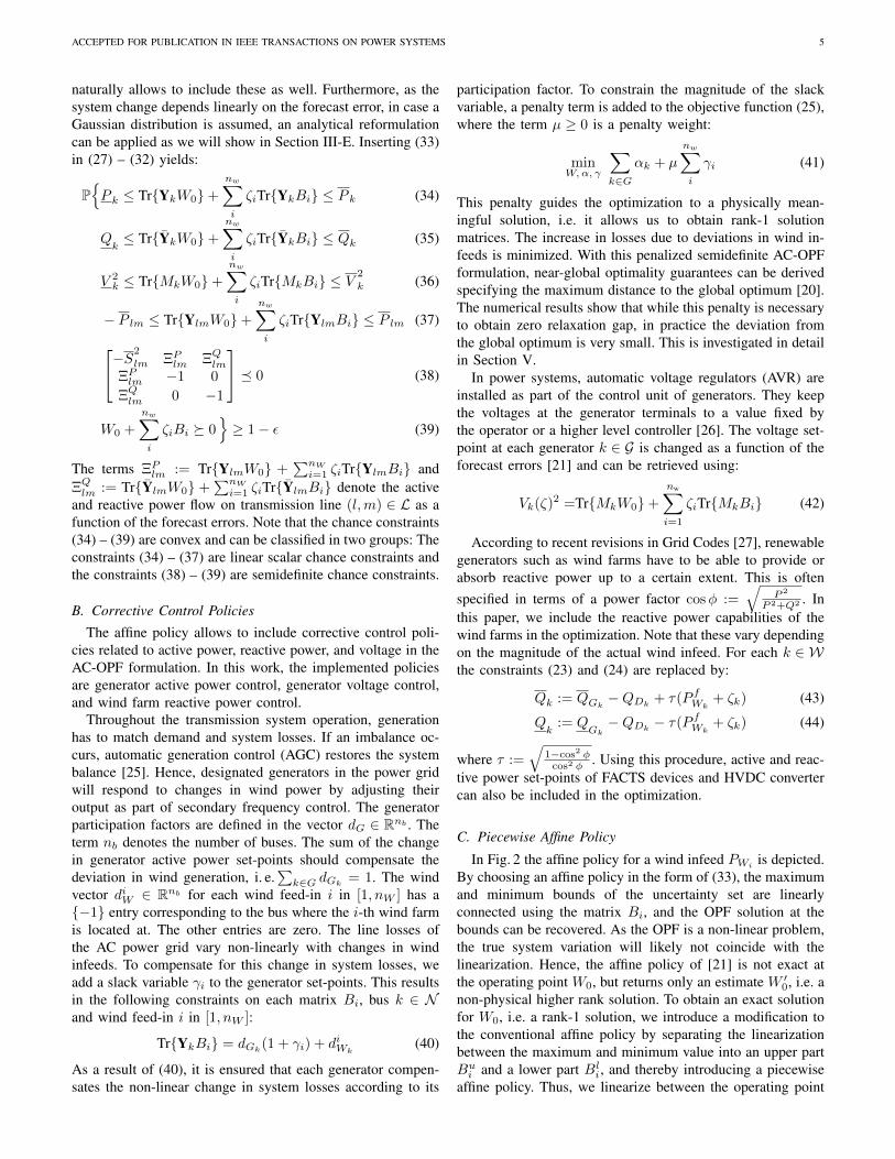
C. Piecewise Affine Policy

In Fig. 2 the affine policy for a wind infeed PWi is depicted.By choosing an affine policy in the form of (33), the maximumand minimum bounds of the uncertainty set are linearlyconnected using the matrix Bi, and the OPF solution at thebounds can be recovered. As the OPF is a non-linear problem,the true system variation will likely not coincide with thelinearization. Hence, the affine policy of [21] is not exact atthe operating point W0, but returns only an estimate W ′0, i.e. anon-physical higher rank solution. To obtain an exact solutionfor W0, i.e. a rank-1 solution, we introduce a modification tothe conventional affine policy by separating the linearizationbetween the maximum and minimum value into an upper partBui and a lower part Bli, and thereby introducing a piecewiseaffine policy. Thus, we linearize between the operating point

ACCEPTED FOR PUBLICATION IN IEEE TRANSACTIONS ON POWER SYSTEMS 6

PWi

System change

W0

W ′0

BiBu

i

Bli

W0 + ζiBui

W ′0 + ζiBi

W0 + ζiBl

i

W ′0 + ζ

iBi

P fWi

+ ζi

P fWi

P fWi

+ ζi

Fig. 2. Piecewise affine policy: The linearization between upper and lowerlimit is split into two corresponding piecewise linearizations starting fromthe exact operating point W0. The red line indicates the true system behaviorand the dashed lines the approximation which is made with the correspondingaffine policy. This modification allows us to obtain the exact rank-1 solutionW0, not the higher-rank approximation W ′

0.

and the maximum and minimum value of the uncertainty set,respectively. We extend the work of [21], by ensuring that theobtained solution is exact at the operating point. An additionalbenefit of our approach is that we get a closer approximationof the true system behavior, while the obtained control policiesare piecewise linear.

D. Tractable Formulation for Rectangular Uncertainty Set

In this section, we provide a tractable formulation of thechance constraints for a rectangular uncertainty set. The pro-posed procedure is a combination of robust and randomizedoptimization from [22] and which is applied to chance con-strained AC-OPF in [21]. A scenario-based method, whichdoes not make any assumption on the underlying distributionof the forecast errors, is used to compute the bounds ofthe uncertainty set. Two parameters need to be specified,ε ∈ (0, 1) is the allowable violation probability of the chanceconstraints and β ∈ (0, 1) a confidence parameter. Then, theminimum volume hyper-rectangular set is computed, whichwith probability 1− β contains 1− ε of the probability mass.According to [21], it is necessary to include at least thefollowing number of scenarios Ns to specify the uncertaintyset:

Ns ≥1

1− εe

e− 1(ln

1

β+ 2nW − 1) (45)

The term e is Euler’s number. The minimum and maximumbounds on the forecast errors ζi ∈ [ζ

i, ζi] are retrieved by

a simple sorting operation among the Ns scenarios and thevertices, i.e. the corner points, of the rectangular uncertaintyset can be defined.

To obtain a tractable formulation of the chance constraints,the following result from robust optimization is used: Ifthe constraint functions are linear, monotone or convex withrespect to the uncertain variables, then the system variableswill only take the maximum values at the vertices of theuncertainty set [22]. The chance constraints (34) – (37) arelinear and the semidefinite chance constraints (38), (39) are

convex. Hence, it suffices to enforce the chance constraints atthe vertices v ∈ V of the uncertainty set.

The vector ζv ∈ RnW collects the forecast error boundsfor each vertex, i.e. the entries of this vector correspond tothe the deviation of each wind farm for a specific vertex v.For each vertex, a corresponding slack variable γv is defined.Based on our experience with the SDP solvers, we introducethe following more numerically robust formulation:

Wv := W0 +

nW∑i=1

ζviBi (46)

The matrix Wv denotes the power flow solution at the corre-sponding vertex v. The active and reactive power limits foreach bus k ∈ N and vertex v ∈ V can be written as:

Qv

k := QGk−QDk

+ τ(P fWk+ ζvk) (47)

Qvk

:= QGk−QDk

− τ(P fWk+ ζvk) (48)

Pv

k := PGk− PDk

+ P fWk+ ζvk (49)

P vk := PGk− PDk

+ P fWk+ ζvk (50)

We provide a tractable formulation of chance constraints (34)– (39) for each vertex v ∈ V , bus k ∈ N and line (l,m) ∈ L:

P vk ≤ Tr{YkWv} ≤ Pv

k (51)

Qvk≤ Tr{YkWv} ≤ Q

v

k (52)

V 2k ≤ Tr{MkWv} ≤ V

2

k (53)

− P lm ≤ Tr{YlmWv} ≤ P lm (54)[−(Slm)2 Tr{YlmWv} Tr{YlmWv}

Tr{YlmWv} −1 0

Tr{YlmWv} 0 −1

]� 0 (55)

Wv � 0 (56)Tr{Yk(Wv −W0)} =

nW∑i=1

ζvi(dGk(1 + γv) + diWk

) (57)

The constraint (57) links the forecasted system state to eachof the vertices. To enforce the semidefinite chance constraint(39) for the uncertainty set, it suffices that Wv is positivesemidefinite at the vertices of the uncertainty set, i. e. (56)is fulfilled. For illustrative purposes, in Fig. 3 a rectangularuncertainty set is depicted for two uncertain wind infeeds PW1

and PW2. The resulting optimization problem for a rectangular

uncertainty set of dimension nw minimizes the objective (41)subject to constraints (26) and (51) – (57). Note that theproposed formulation holds for an arbitrary high-dimensionalrectangular uncertainty set.

E. Tractable Formulation for Gaussian Uncertainty Set

In the following, it is assumed that the forecast errors ζ arerandom variables following a Gaussian distribution with zeromean and covariance matrix Λ. Assuming a Gaussian distribu-tion can be helpful when there is insufficient amount of data athand, as it can provide a suitable approximation of the powersystem operation under uncertainty. At the same time, throughthe covariance matrix, geographical correlations between windfarms, solar PV plants, or other types of uncertainty can becaptured. We give a direct tractable formulation of the chance

ACCEPTED FOR PUBLICATION IN IEEE TRANSACTIONS ON POWER SYSTEMS 7

PW1

PW2

P fW1

+ ζ1

P fW1

P fW1

+ ζ1

P fW2

P fW2

+ζ2

P fW2

+ζ2

W0

W3 W2

W4 W1

Fig. 3. Rectangular uncertainty set derived from a scenario-based methoddisplayed for two wind farms. It is sufficient to enforce the chance constraintsat the vertices of the uncertainty set. The vertices are denoted with circles.

constrained AC-OPF, as the work in [3] presented for thechance constrained DC-OPF.

For a defined confidence interval 1− ε, the uncertainty setfor a Gaussian distribution of the forecast errors is an ellipsoid.First, the direction of linearization of the B matrices is rotatedto correspond to the ellipsoid axes which are described by theeigenvectors ηi of the covariance matrix. The eigenvalues λidescribe the squared dimension of the ellipsoid in the directionof its axes. Similar to the rectangular uncertainty set, weintroduce the following auxiliary variables for each ellipsoidaxis i in [1, nW ] and bus k ∈ W:

dG := dG||ηi||, diWk:= ηi, ζi :=

√λi (58)

With Bi we denote the matrices of the affine policy rotated inthe direction of the ellipsoid axes and (40) has to hold:

Tr{YkBi} = dGk(1 + γi) + diWk

(59)

Second, we use theoretical results on chance constraints fromthe work in [28], which presents the theory for an analyticalreformulation of linear scalar chance constraints. To applythe reformulation, we approximate the joint probability ofthe chance constraint violation (34)–(39) with the violationprobability of each individual chance constraint, which is con-servative. Applying the reformulation to the chance constraints(34) – (37) yields for each bus k ∈ N and line (l,m) ∈ L:

P k ≤ Tr{YkW0} ±

√√√√ nw∑i

κ2iTr{YkBi}2 ≤ P k (60)

Qk≤ Tr{YkW0} ±

√√√√ nw∑i

κ2iTr{YkBi}2 ≤ Qk (61)

V 2k ≤ Tr{MkW0} ±

√√√√ nw∑i

κ2iTr{MkBi}2 ≤ V

2

k (62)

−P lm ≤ Tr{YlmW0} ±

√√√√ nw∑i

κ2iTr{YlmBi}2 ≤ P lm (63)

PW1

PW2

P fW1

P fW2 (II)

(I)

(III)

(IV)

W0

W0 − κ2Bl2

W0 + κ1Bu1

W0 − κ1Bl1

W0 + κ2Bu2

Fig. 4. Uncertainty set resulting from a Gaussian distribution of the forecasterrors considering correlation. The directions of approximation for the affinepolicy are rotated corresponding to the eigenvectors of the covariance matrix.The circles denote the points for which the definite chance constraint isenforced. As a result, it holds for the whole dotted rectangular shape. Theindices (I) – (IV) denote the four quadrants of the uncertainty set for each ofwhich the complete set of constraints (55), (59) and (60) – (64) is included.

The term κi := Φ−1(1 − ε)ζi is introduced, where Φ−1

denotes the inverse Gaussian function. The chance constraint(39) is a linear matrix inequality which ensures that the matrixW0 +

∑nw

i ζiBi is positive semidefinite inside a confidenceinterval 1 − ε. An analytical reformulation of this type ofconstraint is not known [28]. As a safe approximation, itsuffices to enforce that W0+

∑nw

i ζiBi is positive semidefiniteat maximum corresponding deviations ±κi to ensure that (32)is fulfilled. We include the following semidefinite constraintsfor each ellipsoid axis i ∈ [1, nW ]:

W0 ± κiBi � 0 (64)

This results in (39) holding for the outer rectangular ap-proximation of the ellipsoid uncertainty set. The semidefinitechance constraint on the apparent branch power flow can beconservatively approximated by enforcing it for the smallestrectangular set enclosing the ellipsoid, i.e. by including theconstraint (55) in the optimization.

The assumption of a multivariate Gaussian distribution ofthe forecast errors leads to an uncertainty set which in twodimensions can be described as an ellipse. For the case oftwo wind farms with uncertain infeeds PW1 and PW2 thisconfiguration is depicted in Fig. 4. Incorporating the results onthe modification of the affine policy presented in Section III-C,we add the constraints (60) – (63) not for Bi but for bothBui and Bli and each of their combinations, splitting theuncertainty set into four quadrants (I) – (IV) as depictedin Fig. 4. The resulting optimization problem corresponds tominimizing objective function (41) subject to constraints (26),(55), (59) and (60) – (64) for each quadrant of the ellipsoid.

IV. LINEARIZATION USING PTDFS

In the following, an alternative approach is presented whichis used as benchmark for comparison with the rest of theapproaches presented in this paper. To describe the system

ACCEPTED FOR PUBLICATION IN IEEE TRANSACTIONS ON POWER SYSTEMS 8

change as a function of the forecast errors, in this section weintroduce a linear approximation based on DC power flow.This linear approximation uses the so-called power transferdistribution factors (PTDFs) to estimate the change in lineloading due to a change in active power injections. Thisapproach has been used in the works in [3] and [29] in thecontext of DC- and AC-OPF, respectively.

The PTDFs use the DC power flow representation, i. e.assuming that the voltage magnitudes of all buses are equalto 1 p.u. and the resistances of branches are neglected.Hence, line losses are neglected and the generator participationfactors are defined without including the slack term γ. As weassume constant voltage magnitudes, the semidefinite (32), thevoltage (29) and the reactive power (28) chance constraintsare dropped and the focus is on approximating the chanceconstraints for the active power bus injection and active powerbranch flow, Eqs. (27) and (30). The admittance matrix BDC isconstructed using only the line reactances xlm. The resultingmatrix is singular. Thus, one column and the correspondingrow are removed to obtain BDC. The vectors dG and diWcollect the generator participation factors and wind injections,and dG and diW denote the corresponding vectors with the firstentry removed. The PTDF for each line (l,m) ∈ L is definedas follows:

PTDFlm = (el − em)T 1xlm

B−1DC (65)

The PTDFs provide an approximate linear relation between achange in bus power injections and the change of the activepower flow over a transmission line. Assuming the maximumand minimum bounds of the forecast errors are described by arectangular uncertainty set with vertices ζv from the previouslydescribed scenario-based approach, we formulate a tractableapproximation of (27) and (30) for each bus k ∈ N , line(l,m) ∈ L and vertex v ∈ V:

P vk ≤ Tr{YkW0}+

nW∑i

ζvi(dGk+ diWk

) ≤ P vk (66)

−P lm ≤ Tr{YlmW0}+nW∑i

PTDFlmζvi(dG + diW ) ≤ P lm (67)

Assuming the forecast errors follow a Gaussian distributionwith zero mean and co-variance matrix Λ, we formulate atractable approximation of (27) and (30) for each bus k ∈ Nand line (l,m) ∈ L:

P k ≤ Tr{YkW0} ± Φ−1(1− ε)√d2Gk

1TΛ1 ≤ P k (68)

−P lm ≤ Tr{YlmW0} ± Φ−1(1− ε)√

ΨTΛΨ ≤ P lm (69)

The term 1 ∈ RnW denotes the vectors of ones. The vectorΨ ∈ RnW contains for each wind feedin i ∈ [1, nW ] theapproximated change in line loading:

Ψi = PTDFlm(dG + diW ) (70)

V. SIMULATION AND RESULTS

In this section, we first describe the simulation setup.Subsequently, using the IEEE 24 bus test case, we investigate

the relaxation gap of the obtained solution matrices as afunction of the penalty weight. Detailed results on the IEEE118 bus test case using realistic forecast data are providedand our proposed approaches are compared to two alternativeapproaches described in the literature.

A. Simulation Setup

The optimization problem is implemented in Julia using theoptimization toolbox JuMP [30] and the SDP solver MOSEK8 [31]. A small resistance of 10−4 has to be added to eachtransformer, which is a condition for obtaining zero relaxationgap [15]. To investigate whether the relaxation gap of anobtained solution matrix W is zero, the ratio ρ of the 2nd

to 3rd eigenvalue is computed, a measure proposed by [23].This value should be around 105 or larger for zero relaxationgap to hold, which means that the obtained solution matrixis rank-2. The respective rank-1 solution can be retrieved byfollowing the procedure described in [23]. According to [15],the obtained solution is then a feasible solution to the originalnon-linear AC-OPF problem.

The work in [20] proposes the use of the following measureto evaluate the degree of the near-global optimality of apenalized SDP relaxation. Let f1(x) be the generation costof the convex OPF without a penalty term and f2(x) thegeneration cost of the convex OPF with a penalty weightsufficiently high to obtain rank-1 solution matrices. Then,the near-global optimality can be assessed by computing theparameter δopt := f1(x)

f2(x)·100%. The closer this parameter is to

100%, the closer the solution is to the global optimum. Notethat this distance is an upper bound to the distance from globaloptimality.

B. Investigating the Relaxation Gap

This section investigates the relaxation gap of the obtainedmatrices. With relaxation gap, we refer to the gap between theSDP relaxation and a non-linear chance constrained AC-OPFwhich uses the affine policy to parametrize the solution space.The IEEE 24 bus system with parameters specified in [32]is used. The allowable violation probability is selected to beε = 5%. Two wind farms with a forecasted infeed of 50 MWand 150 MW and a maximum power of 150 MW and 400 MWare introduced at buses 8 and 24, respectively. For illustrativepurposes, the forecast error for the rectangular uncertaintyis assumed to be bounded within ±50% of the forecastedvalue with 95% probability. For the Gaussian uncertainty set,a standard deviation of 25% of the forecasted value andno correlation between both wind farms is assumed. Eachgenerator adjusts its active power proportional to its maximumactive power to react to deviations in wind power output.

For the rectangular uncertainty set, Fig. 5 shows the eigen-value ratios ρ of the matrices W0 −W4 as a function of thepenalty weight µ. A certain minimum value for the weightµ = 175 is necessary to obtain solution matrices with rank-1,i.e. eigenvalue ratio ρ higher than 105, at the operating stateW0 and the four vertices of the rectangular uncertainty setW1 −W4. The near-global optimality at µ = 175 for this testcase evaluates to a tight upper bound of 99.74%. If the penalty

ACCEPTED FOR PUBLICATION IN IEEE TRANSACTIONS ON POWER SYSTEMS 9

0 100 200 300 400

105

1010

Eig

enva

lue

ratio

ρ

ρ(W0)

ρ(W1)

ρ(W2)

ρ(W3)

ρ(W4)

0 100 200 300 400

5.85

5.9 ·104

Cos

t($

/h)

Gen.cost

0 100 200 300 400-200

0

200

Weight for droop penalty µ (p.u.)

Cos

t($

/h)

Penaltyterm

Fig. 5. Eigenvalue ratios ρ, generation cost and penalty term as a function ofthe power loss penalty weight µ for a IEEE 24 bus test case with two windfarms and a rectangular uncertainty set.

0 50 100 150

105

1010

Eig

enva

lue

ratio

ρ

ρ(W0)

ρ(W0 + κ1Bu1 )

ρ(W0 − κ1Bl1)

ρ(W0 + κ2Bu2 )

ρ(W0 − κ2Bl2)

0 50 100 15058,222

58,227

Cos

t($

/h)

Gen.cost

0 50 100 150

3060

Weight for droop penalty µ (p.u.)

Cos

t($

/h)

Penaltyterm

Fig. 6. Eigenvalue ratios ρ, generation cost and penalty term as a function ofthe power loss penalty weight µ for a IEEE 24 bus test case with two windfarms and a Gaussian uncertainty set.

weight is increased beyond µ = 375 a higher rank solution isobtained for the forecasted system state.

A similar observation can be made if a Gaussian distributionis assumed for the forecast errors. Fig. 6 shows the eigenvalueratios ρ as a function of the penalty weight µ for the Gaussianuncertainty set. A certain minimum value for the weight µ =10 is necessary to obtain solution matrices with rank-1 at theoperating state W0 and the four end-point of the ellipsoid axes.The generation cost is almost flat with respect to increasingpenalty weight and the near-global optimality at µ = 10 forthis test case evaluates to an upper bound larger than 99.99%.As it is also observed, the necessary magnitude of the penaltyweight µ to obtain rank-1 solution matrices depends on thetest case and configuration.

C. IEEE 118 Bus Test Case

In this section, our proposed approaches using the affine pol-icy and PTDFs are compared with two alternative approachesdescribed in the literature [5], [12]. We use the IEEE 118 bus

1 2 3 4 50

0.2

0.4

0.6

0.8

1

P W1

(p.u

.)

BoundsForecast

1 2 3 4 50

0.2

0.4

0.6

0.8

1

Time (h)

P W2

(p.u

.)

BoundsForecast

Fig. 7. Forecast data from hour 1 to hour 5. The bounds correspond tothe minimum and maximum values from the Ns sampled scenarios for therectangular uncertainty set.

0.4 0.6 0.8 1

0.4

0.6

0.8

1

PW1 (p.u.)

PW

2(p

.u.)

RectangularGaussianSamples

Fig. 8. Comparison of rectangular and Gaussian uncertainty set obtained fromthe Ns scenarios sampled for hour 4.

test case with realistic forecast data for the wind farms, andMonte Carlo simulations to evaluate the constraint violations.

1) Simulation Setup: We use the IEEE 118 bus specifi-cations from [33] with the following modifications: The busvoltage limits are set to 0.94 p.u. and 1.06 p.u. As the upperbranch flow limits are specified in MW, the active line flowlimit is considered for branch flows. The line flow limits aredecreased by 30% and the load is increased by 30% to obtain amore constrained system. Two wind farms with a rated powerof 300 MW and 600 MW are placed at buses 5 and 64. Therated wind power corresponds to 24.1% of total load demand.Realistic day-ahead wind forecast scenarios from [34] and [35]are used for both wind farms. To create the scenarios, themethodology described in [34] is used. The forecasts are basedon wind power measurements in the Western Denmark areafrom 15 different control zones collected by the Danish trans-mission system operator Energinet. We select control zone 1to correspond to the wind farm at bus 5 and zone 7 to the windfarm at bus 64. We allow a constraint violation of ε = 5% forall considered approaches. In order to construct the rectangularuncertainty set, the confidence parameter β = 10−3 is selected.Then, a minimum of 314 scenarios are required according to(45). The forecast is computed as mean value of the scenarios.For the Gaussian uncertainty set, we compute the co-variancematrix based on these 314 scenarios. Fig. 7 shows the forecastdata from hour 1 to hour 5 with the upper and lower boundsspecified by the maximum and minimum scenario values,

ACCEPTED FOR PUBLICATION IN IEEE TRANSACTIONS ON POWER SYSTEMS 10

respectively. In Fig. 8 the rectangular and Gaussian uncertaintyset for hour 4 are shown.

In the following, the parameters for the corrective controlpolicies are specified. A participation factor of 0.25 isselected for the generators at buses i = {12, 26, 54, 61}, i.e.dGi

= 0.25. Wind farms have a reactive power capability of0.95 inductive to 0.95 capacitive according to recent GridCodes [27]. The approaches using PTDFs assign a fixedpower factor cosφ to each wind farm. The affine policyincludes a generator voltage and wind farm reactive powercorrective control, assigning an updated set-point to generatorsand wind farms based on the actual realization of the forecasterrors. To facilitate comparability, we use the same scenariosfor all approaches to compute the respective uncertainty sets.We evaluate the constraint violations using Monte Carlosimulations with 10’000 scenarios and MATPOWER ACpower flows [32]. We enable the enforcement of generatorreactive power limits in the power flow, i.e. PV busesare converted to PQ buses once the limits are reached, asotherwise high nonphysical overloading of the limits canoccur [36]. Furthermore, we distribute the loss mismatchfrom the active generator set-points among the generatorsaccording to their participation factors and rerun the powerflow to mimic the response of automatic generation control(AGC).

2) Numerical Comparison to Alternative Approaches: Inthe following, the main modeling assumptions of the respectiveapproaches and the type of chance constraints they includeare outlined. All approaches considering chance constraintsinclude corrective control of the active generator set-points.

• Chance constrained DC-OPF [5] (DC-OPF): A robust for-mulation based on DC-OPF includes chance constraintson active generator power and active branch flow. Intervalbounds on the forecast errors are assumed. Hence, we usethe scenarios to compute the interval bounds. A powerfactor of 1 is assumed for wind farms.

• Iterative chance constrained AC-OPF [12] (Iterative): Ateach iteration the Jacobian is computed and the un-certainty margins resulting from the chance constraintsare updated until convergence is reached. The forecasterrors are assumed to follow a Gaussian distribution. Thecovariance matrix constructed from the Ns scenarios isused. Chance constraints on active and reactive generatorlimits, voltage magnitudes and apparent line flows areincluded in the formulation. A power factor of 1 isassumed for wind farms, as no reactive power correctivecontrol is included in [12].

These two approaches are compared to the following ap-proaches based on the formulations presented in this work:

• AC-OPF with convex relaxations but without chanceconstraints (AC-OPF) [15]

• Chance constrained AC-OPF with convex relaxations,using an affine policy for a Gaussian uncertainty set(AP (Gauss)) including corrective control for wind farms,generator voltages and generator active power.

• Chance constrained AC-OPF with convex relaxations,

TABLE IICOST OF UNCERTAINTY: GENERATION COST IN RELATION TO AC-OPF

WITH CONVEX RELAXATIONS WITHOUT CONSIDERATION OFUNCERTAINTY

Time step (h) 1 2 3 4 5

AP (Rect) (%) 0.774 0.740 0.755 0.921 1.562

PTDF (Rect) (%) 0.785 0.748 0.767 0.931 1.588

DC-OPF [5] (%) -2.782 -2.826 -2.824 -2.673 -2.165

AP (Gauss) (%) 0.515 0.461 0.467 0.489 0.512

PTDF (Gauss) (%) 0.523 0.468 0.477 0.497 0.520

Iterative [12] (%) 0.519 0.465 0.473 0.494 0.516

using an affine policy for a rectangular uncertainty set(AP (Rect)) including corrective control for wind farmsand generator voltages and generator active power.

• Chance constrained AC-OPF with convex relaxations,using PTDFs (PTDF (Gauss)) for a Gaussian uncertaintyset.

• Chance constrained AC-OPF with convex relaxations,using PTDFs (PTDF (Rect)) for a rectangular uncertaintyset.

In Table II the cost of uncertainty for the different approachesand considered time steps are shown. The cost of uncertaintyrepresents the additional cost incurred by considering thestochastic variables, and is defined as the difference betweenthe solution of the chance constrained and a baseline. Inthis paper, the AC-OPF with convex relaxations but withoutconsidering uncertainty is assumed as the baseline cost. FromTable II, we make the following observations. First, the DC-OPF (with chance constraints) leads to a cost reduction, as nolosses are considered compared to the AC-OPF. Second, theapproaches stemming from robust optimization lead to a costincrease of approximately 0.8% for time step 1 compared toan increase of approximately 0.5% for the same time stepfor the approaches assuming a Gaussian distribution. Thisshows that the Gaussian uncertainty set is less conservativeas indicated in Fig. 8. For the rectangular uncertainty set,the affine policy reduces the cost compared to the approachusing PTDFs. Comparing the approaches for the Gaussianuncertainty set, again the affine policy results to the lowestcost of uncertainty compared to the approach using PTDFsand the iterative chance constrained AC-OPF. The reason forthat is that the affine policy includes corrective control forvoltages and both active and reactive power.

In Table III the violation probability of the chance con-straints on active power, voltages, and active branch flowsare shown. Monte Carlo simulations using 10’000 scenarioswith MATPOWER AC power flows are conducted. A mini-mum violation limit of 10−3 p.u. for active generator limitsand 0.1% for voltage and line flow limits is considered toexclude numerical errors. In all considered time steps, the AC-OPF without consideration of uncertainty leads to insecureinstances and violates constraints on line and generator limitson active power.

First, investigating the robust approaches using the rectangu-

ACCEPTED FOR PUBLICATION IN IEEE TRANSACTIONS ON POWER SYSTEMS 11

TABLE IIIVIOLATION PROBABILITY OF THE CHANCE CONSTRAINTS ON BUS

VOLTAGE, ACTIVE BRANCH FLOW AND ACTIVE GENERATOR POWER FORTHE FORECAST DATA. MONTE CARLO SIMULATIONS USING 10’000

SCENARIOS WITH MATPOWER AC POWER FLOWS ARE CONDUCTED.INSECURE INSTANCES ARE MARKED IN BOLD.

Time step (h) 1 2 3 4 5

Bus voltage

AC-OPF (%) 0.0 0.1 0.2 1.0 4.3

DC-OPF [5] (%) 100.0 100.0 100.0 100.0 100.0

PTDF (Rect) (%) 19.5 20.9 14.6 13.0 12.9

AP (Rect) (%) 0.0 0.0 0.0 0.0 0.0

PTDF (Gauss) (%) 20.0 21.2 15.0 13.5 13.0

AP (Gauss) (%) 0.7 1.9 4.3 7.2 7.6

Iterative [12] (%) 0.0 0.0 0.0 0.0 0.0

Active power line limit

AC-OPF (%) 17.7 18.8 14.9 32.5 46.5

DC-OPF [5] (%) 0.0 0.0 0.0 2.8 0.0

PTDF (Rect) (%) 0.0 0.0 0.0 0.0 0.0

AP (Rect) (%) 0.0 0.0 0.0 0.0 0.0

PTDF (Gauss) (%) 4.6 11.1 13.1 9.3 7.8

AP (Gauss) (%) 4.6 3.7 0.9 2.6 5.8

Iterative [12] (%) 1.6 2.0 3.6 4.2 5.3

Active generator limit

AC-OPF (%) 46.4 48.8 45.9 45.5 40.9

DC-OPF [5] (%) 34.3 38.6 30.1 14.5 2.0

PTDF (Rect) 0.0 0.0 0.0 0.0 0.0

AP (Rect) (%) 0.0 0.0 0.0 0.0 0.0

PTDF (Gauss) (%) 2.6 3.6 2.8 3.1 5.5

AP (Gauss) (%) 0.0 0.2 0.4 2.3 0.7

Iterative [12] (%) 2.9 4.1 3.0 3.3 5.7

lar uncertainty set the following observations can be made: Therobust DC-OPF formulation in [5] leads to insecure instancesfor all time steps and violates both voltage and generator activepower constraints. The AC-OPF approach using PTDFs forthe chance constraints reduces the voltage violations but doesnot comply with the 5% confidence interval. The AC-OPFusing the affine policy complies with the chance constraintsfor all time steps while slightly decreasing the generationcost compared to the approach using PTDFs. As the scenariobased method is conservative, there are nearly zero violationsoccurring for the considered 10’000 samples for the approachusing the affine policy.

Second, we compare the different approaches which assumea Gaussian distribution of the forecast errors. The affine policyimproves upon the approach using PTDFs and results to asecure operation for time steps 1 to 3. For time steps 4 and 5we observe a slight violation of the active power line and busvoltage limit. This is due to the fact that we do not sample outof a Gaussian distribution but out of a set of realistic forecastscenarios, that apparently are not Gaussian distributed. The

TABLE IVCOMPARISON OF VIOLATION PROBABILITY OF THE CHANCE

CONSTRAINTS ON BUS VOLTAGE, ACTIVE BRANCH FLOW AND ACTIVEGENERATOR POWER FOR AFFINE POLICY AND ITERATIVE AC-OPF WITH

10’000 SAMPLES FROM A GAUSSIAN DISTRIBUTION.

Time step (h) 1 2 3 4 5

Bus voltage

AP (Gauss) (%) 0.1 0.4 0.5 0.8 0.7

Iterative [12] (%) 0.0 0.0 0.0 0.0 0.0

Active power line limit

AP (Gauss) (%) 2.2 1.7 2.1 2.1 2.1

Iterative [12] (%) 1.5 1.7 1.7 2.1 2.1

Active generator limit

AP (Gauss) (%) 2.4 2.7 2.7 2.6 2.5

Iterative [12] (%) 2.7 2.6 2.3 2.4 2.1

iterative approach results to a secure operation for time steps1 to 4 and slightly violates the active generator and branchflow limit in time step 5.

In order to verify if these violations occur due to the mis-match between actual distribution and the assumed Gaussianwe repeat the 10’000 scenario evaluations for both affinepolicy and the iterative chance constrained AC-OPF from [12].We sample from the Gaussian distribution assumed for theuncertainty set. The results are shown in Table IV. For all5 time steps, both approaches comply with the 5% violationprobability. Hence, the occurring violations in Table III stemfrom the mismatch between Gaussian distribution and actualprobability distribution. As shown in Table II, the affine policyresults in a slightly lower generation cost than the iterative AC-OPF, as it includes corrective control policies. This leads usto the following conclusions. First, that if the forecast errorsdo follow a normal distribution both approaches demonstrategood performance and do not exceed the violation limit. If thedata are not normally distributed, as is the case for the resultsshown in Table III, none of the two methods can guaranteethat the violation probability will be below ε. The differencesin performance in that case are, as it would be expected, data-and system-specific. However, independent from the fact ifthe underlying probability distribution is Gaussian or not, onedifference that remains is that the approach proposed in thispaper is more rigorous, since it provides guarantees regardingthe global optimality of the obtained solution and allows toinclude corrective control policies related to reactive powerand voltage.

Table V lists the penalty weights and obtained near-globaloptimality guarantees for the 5 time steps. Note that it issufficient to define for both uncertainty sets a penalty weight ofµ = 100 p.u. to obtain zero relaxation gap, i.e. rank-1 solutionmatrices and a near-global optimality guarantee of larger than99.99%. This means that the maximum deviation from theglobal optimum is smaller than 0.01% of the objective value.

Table VI lists the computational time of the different ap-proaches. The optimization problems are solved on a desktop

ACCEPTED FOR PUBLICATION IN IEEE TRANSACTIONS ON POWER SYSTEMS 12

TABLE VPOWER LOSS PENALTY WEIGHT AND NEAR-GLOBAL OPTIMALITY

GUARANTEES FOR IEEE 118 BUS TEST CASE FOR ALL CONSIDERED TIMESTEPS

Penalty weight µ Near-global optimality(p.u.) guarantee δopt (%)

AP (Rect) 100 ≥ 99.99

AP (Gauss) 100 ≥ 99.99

TABLE VISOLVING TIME FOR IEEE 118 BUS TEST CASE

AP (Rect) AP (Gauss) PTDF (Rect)

30 sec 10 min 15 sec

PTDF (Gauss) DC-OPF [5] Iterative [12]

15 sec ≤ 1 sec 4 sec

computer with an Intel Xeon CPU E5-1650 v3 @ 3.5 GHz and32 GB RAM. For all optimization problems except the iterativeapproach, MOSEK V8 [31] is used. The iterative approachutilizes the MATPOWER AC-OPF. The DC-OPF formulationis the fastest, as the optimization problem is a linear program.The computational time increases with increasing constraintcomplexity. The SOC constraints in the formulation for theGaussian uncertainty set are computationally the most chal-lenging. We observe that the iterative approach, despite theneed for computing a number of iterations, converges fasterthan all approaches that utilize convex relaxations and anSDP solver. Current trends expect the need of more rigorousoptimal power flow approaches in the future, that e.g. canguarantee a global minimum. In that case the need for furtherresearch to improve both the optimization solvers and theconvex formulations of the AC-OPF problem is apparent.Possible directions to increase the computational speed of theproposed approaches are the chordal decomposition technique,outlined in [23], and distributed optimization techniques, e.g.the alternating direction method of multipliers (ADMM) forsparse semidefinite problems in [37]. The chordal decompo-sition technique can be applied to reduce the computationalburden of the semidefinite constraints on W0 and Bi (18). Asshown in [38] a speed-up by several orders of magnitude canthen be expected for large systems.

VI. CONCLUSIONS

In this work, a convex formulation for a chance constrainedAC-OPF is presented which is able to provide near-globaloptimality guarantees. The OPF formulation considers chanceconstraints for all relevant variables, and has an explicitrepresentation of corrective control policies. Two tractableformulations are proposed: First, a scenario-based methodis applied in combination with robust optimization. Second,assuming a Gaussian distribution of forecast errors, we providean analytical reformulation of the chance constraints. Detailedcase studies on the IEEE 24 and 118 bus test systems arepresented. For the latter, we used realistic forecast data and

Monte Carlo simulations to evaluate constraint violations.Compared to a chance constrained DC-OPF formulation,we find that the formulations proposed in this paper aremore accurate and significantly decrease constraint violations.Compared with iterative non-convex AC-OPF formulations,both our piece-wise affine control policy and the iterativeAC-OPF do not exceed the constraint violation limit forthe Gaussian uncertainty set. Most importantly, our proposedapproach obtains tight near-global optimality guarantees whichensure that the distance to the global optimum is smaller than0.01% of the objective value. In our future work, besidesinvestigating chordal decomposition techniques, we includesecurity constraints in the proposed formulation by defininga matrix W s(ζ) for each outage s of a generation unit ortransmission line.

ACKNOWLEDGMENT

The authors would like to thank Pierre Pinson for sharingthe forecast data, Line Roald for providing an updated versionof the code from [12], and Martin S. Andersen and Daniel K.Molzahn for fruitful discussions.

REFERENCES

[1] A. Nemirovski and A. Shapiro, “Convex approximations of chanceconstrained programs,” SIAM Journal on Optimization, vol. 17, no. 4,pp. 969–996, 2006.

[2] D. Bienstock, M. Chertkov, and S. Harnett, “Chance-constrained optimalpower flow: Risk-aware network control under uncertainty,” SIAMReview, vol. 56, no. 3, pp. 461–495, 2014.

[3] L. Roald, F. Oldewurtel, T. Krause, and G. Andersson, “Analytical refor-mulation of security constrained optimal power flow with probabilisticconstraints,” in IEEE PowerTech, Grenoble, France, 2012.

[4] M. Lubin, Y. Dvorkin, and S. Backhaus, “A robust approach to chanceconstrained optimal power flow with renewable generation,” IEEETransactions on Power Systems, vol. 31, no. 5, pp. 3840 – 3849, 2016.

[5] R. A. Jabr, S. Karaki, and J. A. Korbane, “Robust multi-period OPF withstorage and renewables,” IEEE Transactions on Power Systems, vol. 30,no. 5, pp. 2790–2799, 2015.

[6] L. Roald, S. Misra, T. Krause, and G. Andersson, “Corrective control tohandle forecast uncertainty: A chance constrained optimal power flow,”IEEE Transactions on Power Systems, vol. 32, no. 2, pp. 1626–1637,2017.

[7] S. S. Guggilam, E. Dall’Anese, Y. C. Chen, S. V. Dhople, and G. B.Giannakis, “Scalable optimization methods for distribution networkswith high PV integration,” IEEE Transactions on Smart Grid, vol. 7,no. 4, pp. 2061 – 2070, 2016.

[8] K. Baker, E. Dall’Anese, and T. Summers, “Distribution-agnosticstochastic optimal power flow for distribution grids,” in North AmericanPower Symposium (NAPS), Denver, US, 2016.

[9] T. Summers, J. Warrington, M. Morari, and J. Lygeros, “Stochastic opti-mal power flow based on convex approximations of chance constraints,”in 2014 Power Systems Computation Conference, 2014.

[10] E. D. Anese, K. Baker, and T. Summers, “Chance-constrained ACoptimal power flow for distribution systems with renewables,” IEEETransactions on Power Systems, vol. PP, no. 99, pp. 1–1, 2017.

[11] H. Zhang and P. Li, “Chance constrained programming for optimalpower flow under uncertainty,” IEEE Transactions on Power Systems,vol. 26, no. 4, pp. 2417–2424, 2011.

[12] J. Schmidli, L. Roald, S. Chatzivasileiadis, and G. Andersson, “Stochas-tic AC optimal power flow with approximate chance-constraints,” inIEEE Power and Energy Society General Meeting, Boston, US, 2016.

[13] K. Dvijotham and D. K. Molzahn, “Error bounds on the DC power flowapproximation: A convex relaxation approach,” in IEEE 55th Conferenceon Decision and Control (CDC), 2016, pp. 2411–2418.

[14] S. V. Dhople, S. S. Guggilam, and Y. C. Chen, “Linear approximationsto AC power flow in rectangular coordinates,” in 53rd Annual AllertonConference on Communication, Control, and Computing, 2015, pp. 211–217.

ACCEPTED FOR PUBLICATION IN IEEE TRANSACTIONS ON POWER SYSTEMS 13

[15] J. Lavaei and S. H. Low, “Zero duality gap in optimal power flowproblem,” IEEE Transactions on Power Systems, vol. 27, no. 1, pp.92–107, 2012.

[16] R. A. Jabr, “A conic quadratic format for the load flow equations ofmeshed networks,” IEEE Transactions on Power Systems, vol. 22, no. 4,pp. 2285–2286, 2007.

[17] X. Bai, H. Wei, K. Fujisawa, and Y. Wang, “Semidefinite programmingfor optimal power flow problems,” International Journal of ElectricalPower & Energy Systems, vol. 30, no. 6, pp. 383–392, 2008.

[18] M. B. Cane, R. P. O’Neill, and A. Castillo, “History of optimal powerflow and formulations,” Federal Energy Regulatory Commission, 2012.

[19] B. C. Lesieutre, D. K. Molzahn, A. R. Borden, and C. L. DeMarco,“Examining the limits of the application of semidefinite programmingto power flow problems,” in 49th Annual Allerton Conference onCommunication, Control, and Computing, 2011, pp. 1492–1499.

[20] R. Madani, S. Sojoudi, and J. Lavaei, “Convex relaxation for optimalpower flow problem: Mesh networks,” IEEE Transactions on PowerSystems, vol. 30, no. 1, pp. 199–211, 2015.

[21] M. Vrakopoulou, M. Katsampani, K. Margellos, J. Lygeros, and G. An-dersson, “Probabilistic security-constrained AC optimal power flow,” inIEEE PowerTech, Grenoble, France, 2012.

[22] K. Margellos, P. Goulart, and J. Lygeros, “On the road between robustoptimization and the scenario approach for chance constrained optimiza-tion problems,” IEEE Transactions on Automatic Control, vol. 59, no. 8,pp. 2258–2263, 2014.

[23] D. K. Molzahn, J. T. Holzer, B. C. Lesieutre, and C. L. DeMarco,“Implementation of a large-scale optimal power flow solver basedon semidefinite programming,” IEEE Transactions on Power Systems,vol. 28, no. 4, pp. 3987–3998, 2013.

[24] A. Ben-Tal and A. Nemirovski, “Selected topics in robust convexoptimization,” Mathematical Programming, vol. 112, no. 1, pp. 125–158, 2008.

[25] Ibraheem, P. Kumar, and D. P. Kothari, “Recent philosophies of auto-matic generation control strategies in power systems,” IEEE Transac-tions on Power Systems, vol. 20, no. 1, pp. 346–357, 2005.

[26] H. Vu, P. Pruvot, C. Launay, and Y. Harmand, “An improved voltagecontrol on large-scale power system,” IEEE Transactions on PowerSystems, vol. 11, no. 3, pp. 1295–1303, 1996.

[27] M. Tsili and S. Papathanassiou, “A review of grid code technicalrequirements for wind farms,” IET Renewable Power Generation, vol. 3,no. 3, pp. 308–332, 2009.

[28] A. Nemirovski, “On safe tractable approximations of chance con-straints,” European Journal of Operational Research, vol. 219, no. 3,pp. 707–718, 2012.

[29] S. Chatzivasileiadis, T. Krause, and G. Andersson, “Flexible AC trans-mission systems (FACTS) and power system security - A valuationframework,” in IEEE Power and Energy Society General Meeting,Detroit Michigan, US, 2011.

[30] M. Lubin and I. Dunning, “Computing in operations research usingJulia,” INFORMS Journal on Computing, vol. 27, no. 2, pp. 238–248,2015.

[31] MOSEK ApS, MOSEK 8.0.0.37, 2016.[32] R. D. Zimmerman, C. E. Murillo-Sanchez, and R. J. Thomas, “MAT-

POWER: Steady-state operations, planning, and analysis tools for powersystems research and education,” IEEE Transactions on Power Systems,vol. 26, no. 1, pp. 12–19, 2011.

[33] “IEEE 118-bus, 54-unit, 24-hour system,” Electrical and ComputerEngineering Department, Illinois Institute of Technology, Tech. Rep.[Online]. Available: http://motor.ece.iit.edu/data/JEAS IEEE118.doc

[34] P. Pinson, “Wind energy: Forecasting challenges for its operationalmanagement,” Statistical Science, pp. 564–585, 2013.

[35] W. A. Bukhsh, C. Zhang, and P. Pinson, “An integrated multiperiod OPFmodel with demand response and renewable generation uncertainty,”IEEE Transactions on Smart Grid, vol. 7, no. 3, pp. 1495–1503, 2016.

[36] A. E. Efthymiadis and Y. H. Guo, “Generator reactive power limits andvoltage stability,” in Fourth International Conference on Power SystemControl and Management (Conf. Publ. No. 421), 1996, pp. 196–199.

[37] R. Madani, A. Kalbat, and J. Lavaei, “ADMM for sparse semidefiniteprogramming with applications to optimal power flow problem,” in 54thIEEE Conference on Decision and Control (CDC), 2015, pp. 5932–5939.

[38] R. A. Jabr, “Exploiting sparsity in SDP relaxations of the OPF problem,”IEEE Transactions on Power Systems, vol. 27, no. 2, pp. 1138–1139,2012.

Andreas Venzke (S’16) received the M.Sc. degree inEnergy Science and Technology from ETH Zurich,Zurich, Switzerland in 2017. He is currently work-ing towards the Ph.D. degree at the Departmentof Electrical Engineering, Technical University ofDenmark (DTU), Kongens Lyngby, Denmark. Hisresearch interests include power system operationunder uncertainty and convex relaxations of optimalpower flow.

Lejla Halilbasic (S’15) received the M.Sc. degreein Electrical Engineering from the Technical Uni-versity of Graz, Austria in 2015. She is currentlyworking towards the Ph.D. degree at the Departmentof Electrical Engineering, Technical University ofDenmark (DTU), Denmark. Her research interestsinclude optimization of power system operation andits applications to electricity markets.

Uros Markovic (S’16) received the M.Sc. degree inElectrical Engineering and Information Technologyfrom ETH Zurich, Zurich, Switzerland in 2016. Heis currently working towards the Ph.D. degree at thePower Systems Laboratory, ETH Zurich, where hejoined in March 2016. His research interests includemodeling, control and optimization of inverter-basedpower system with low rotational inertia.

Gabriela Hug (S’05, M’08, SM’14) was born inBaden, Switzerland. She received the M.Sc. degreein electrical engineering in 2004 and the Ph.D.degree in 2008, both from Swiss Federal Institute ofTechnology (ETH), Zurich, Switzerland. After thePh.D. degree, she worked in the Special StudiesGroup of Hydro One, Toronto, ON, Canada, andfrom 2009 to 2015, she was an Assistant Professorin Carnegie Mellon University, Pittsburgh, PA, USA.She is currently an Associate Professor in the PowerSystems Laboratory, ETH Zurich. Her research is

dedicated to control and optimization of electric power systems.

Spyros Chatzivasileiadis (S’04, M’14) is an Assis-tant Professor at the Technical University of Den-mark (DTU). Before that he was a postdoctoralresearcher at the Massachusetts Institute of Technol-ogy (MIT), USA and at Lawrence Berkeley NationalLaboratory, USA. Spyros holds a PhD from ETHZurich, Switzerland (2013) and a Diploma in Elec-trical and Computer Engineering from the NationalTechnical University of Athens (NTUA), Greece(2007). In March 2016 he joined the Center ofElectric Power and Energy at DTU. He is currently

working on power system optimization and control of AC and HVDC grids,including semidefinite relaxations, distributed optimization, and data-drivenstability assessment.